1

Control Flow Visualization of Python

Vijay Kumar Suryadevara Department of Computer Science

New Mexico State University Las Cruces, NM 88001 vsuryade@cs.nmsu.edu

Advisor: Dr. Clinton Jeffery

2

Abstract

This project aims to visualize the control flow of Python programs. It has the

potential to make debugging easier and to help in performance tuning. The visualizations

also help in understanding the program behavior. Profiling and tracing facilities provided

by the Python Interpreter are used in tracing the events of the user program. Python

doesn’t support graphics on its own. VPython graphics package is used to draw the

visualizations. Two visualization tools are designed in this project. The first one

visualizes control flow in a program at line level and the other one at the function/method

call level. The line level visualization is a 3-dimensional plot with line number being

executed as y-coordinate, final event in the current call as x-coordinate and the stack

depth as z-coordinate. The function/method call visualization shows the control flow in a

program using arrow and sphere objects. The functions and classes in a program are

represented by sides of a polygon and the calls between them are represented by arrows

from caller to called. Recursive calls are represented using sphere objects.

3

1. Introduction

Program visualization is a promising area of software engineering and is a branch

of software visualization. Program visualization is a process of depicting the dynamic

behavior of an executing program by continuously updating a graphic display or

representing the program’s control and/or data with the help of graphics at a particular

moment1. Several important applications of program visualization include debugging,

performance tuning, and the study of algorithms.

Control flow visualization is a part of program visualization which deals with

graphical representation of control in a program. This project is about control flow

visualization of Python programs. Python is an interpreted, interactive, object oriented

programming language 2. This work aims to visualize the control flow in Python

programs with the goal of making debugging easier and improving the performance.

The sys module of Python has functions for enabling profiling and tracing

functions 3. There is also a low-level support for attaching profiling and execution tracing

facilities in Python. The Python Interpreter provides a C interface that allows profiling or

tracing code by making a direct C function call instead of calling through Python-level

callable objects 4. Python-level hooks take 60 – 70% more time when compared to the

hooks provided by C interface for event tracing. More information about tracing and

profiling hooks provided by the sys module and the C interface of Python is present in

Appendix A.

One of the limitations of using Python’s built-in tracing facilities is that it is

difficult to visualize the control flow at expression level as these hooks don’t provide any

information of expression-evaluation. The tracing facilities can only provide information

up to the line-level.

Two visualization tools are developed in this project. The first tool uses the C

interface provided by the Python Interpreter for enabling the trace function. The second

tool includes a 3D-visualization and 2D-visualization which uses Python level profiling

facilities. Attempts to use the C interface for setting profiling function failed in the

second visualization tool. The reason for it is described in the Limitations section.

Graphics output is not supported by Python on its own. VPython 5 is used as the

graphics package for the control flow visualization. VPython consists of a graphics

4

module called Visual, developed by David Scherer in 2000 when he was a sophomore at

Carnegie Mellon University. Visual reflects the current positions of objects by refreshing

a 3D scene many times per second 5. The programmer can zoom and rotate a 3D scene

easily with the help of a mouse.

VPython was selected over other graphics packages because of the presence of

high level objects like sphere, arrow, and curve that can be readily used. Appendix B lists

the objects used from VPython and has brief notes on each of this object.

The next section describes the first tool which visualizes control flow at line-

level. It describes the tracing hooks used, implementation of LineTracer module,

visualization program Graph.py and also presents some screenshots. Section 3 presents

the second tool which visualizes the interaction between the functions, classes and

methods of a source program. It introduces the profiling hooks used, implementation of

Visualizer module, CallGraph module, CallGraph2D module. Section 4 presents

interesting screenshots. Limitations of this project are discussed in Section 5. Section 6

concludes the paper.

2. Line level Visualization

This visualization is a 3-dimensional plot with number of events in a call as x-

axis, line number being executed as y-axis and stack depth as z-axis. All the line, call

and return events occurring in a source program are plotted in this visualization. Each of

the events is represented using a sphere object.

Before executing the source program, user has to import LineTracer module in his

program. LineTracer is a Python extension module written in C to trace the events

occurring in a program. It uses the Python’s C interface for tracing the events.

There are two steps of execution for visualizing control flow in the user program.

First the user has to execute the source program after importing LineTracer.

python ProgramName.py

A log file LineEvents.txt is created as a result of this step. The next step is to execute

Graph.py which uses this log file to show the visualization.

python Graph.py

5

2.1 LineTracer

LineTracer is a Python extension module written in C for tracing events in a

program. It uses the profiling and tracing hooks provided by the C interface of the Python

Interpreter. It is written using the Python’s API 6 (Application Programmers Interface)

which defines a set of functions, macros and variables that provide access to most aspects

of the Python to support extension of Python.

LineTracer installs a trace function, TraceEvents. The Interpreter calls

TraceEvents after every line, call, return, and exception event with corresponding

parameters. TraceEvents extracts the required information for visualizing the control flow

from these parameters and writes it into a log file LineEvents.txt. Information from this

log file is used by Graph.py to plot the visualization.

The user has to import LineTracer module in his program and call the

TraceInstaller( ) with the name of source program as parameter in order to trace the

events.

import LineTracer

LineTracertrace.TraceInstaller (programName)

The TraceInstaller( ) uses programName to limit the trace to present program and stop it

from entering the other imported modules.

TraceInstaller( ) installs the trace function TraceEvents( ) using PyEval_SetTrace

statement.

PyEval_SetTrace ((Py_tracefunc) TraceEvents, (PyObject *) self);

int TraceEvents (PyObject *obj, PyFrameObject *f, int what, PyObject *args)

An array of counters, stack[ ], is maintained to keep track of call-stack depth and

the number events in the current call at every instance. The index of the array at each

instance gives the stack depth at that instance whereas the value in the array at this index

gives the number of line events in this call. When a new call is entered the index of the

array is increased and when a call is returned it is decreased. The value in the array at

current index is increased with every line event.

From the frame object passed by the Interpreter, TraceEvents( ) determines the

line number being executed in the source program and also the method to which the

6

current line belongs. frame->f_lineno is the line number and frame->f_code->co_name

is the function/method name. Appendix A lists the members of frame and code objects

with brief description for each member.

TraceEvents( ) writes the current call-stack depth, line number being executed,

number of events in the current call, function/method name of the current event into a log

file LineEvents.txt.

fprintf ( fptr, "%d,%d,%d,%s\n", stack[index], f->f_lineno, index+1, PyString_AS_STRING (f -

> f_code-> co_name ));

The user has to execute Graph.py to get the control flow visualization. Graph.py

reads the LineEvents.txt and plots the visualization using this information.

2.2 Graph.py

Graph.py plots a 3-dimensional graph with number of events in the current call,

line number in the source code, and stack depth as x, y and z coordinates. The graph is

plotted with the sphere objects in a display window of VPython. Each sphere in the graph

represents an event (line, call, return).

If all the events are plotted, the Graph looks complex and denser which makes it

hard to understand. Hence only function/method call, return and final event in each call

are plotted. Although a sphere is plotted for every event in a call, only the sphere

representing final event in a call is kept and the remaining are deleted.

After all the events are plotted, a user can know the information of an event

represented by a sphere object in the 3D-graph. A left click of the mouse on a sphere

object prints the information of the event represented by it. This information includes

stack depth, line number, number of events in that call and method name. All the

information is printed in the shell. A dictionary object dictMethods is used to keep track

of all the sphere objects plotted.

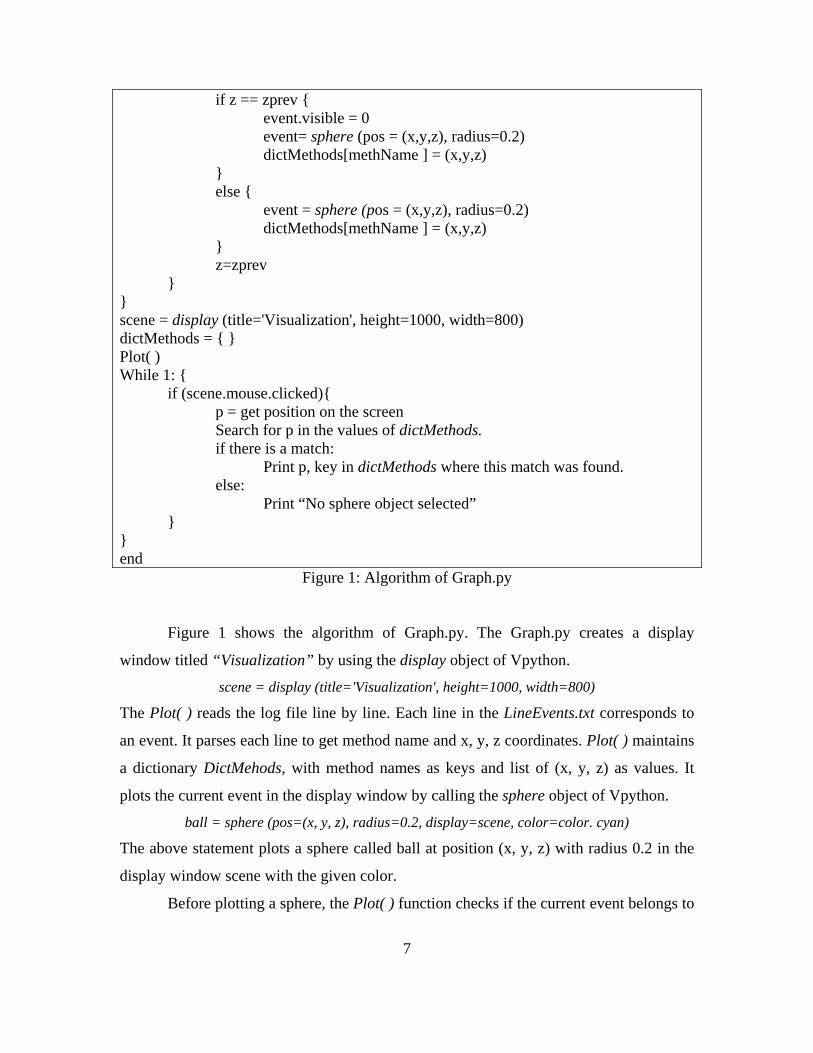
Algorithm Graph.py begin def Plot( ){ zprev = -1 for each line in log file { Parse each line to get x, y, z coordinates and methName.

7

if z == zprev { event.visible = 0 event= sphere (pos = (x,y,z), radius=0.2)

dictMethods[methName ] = (x,y,z) } else { event = sphere (pos = (x,y,z), radius=0.2)

dictMethods[methName ] = (x,y,z) } z=zprev } } scene = display (title='Visualization', height=1000, width=800) dictMethods = { } Plot( ) While 1: {

if (scene.mouse.clicked){ p = get position on the screen Search for p in the values of dictMethods. if there is a match:

Print p, key in dictMethods where this match was found. else:

Print “No sphere object selected” }

} end

Figure 1: Algorithm of Graph.py

Figure 1 shows the algorithm of Graph.py. The Graph.py creates a display

window titled “Visualization” by using the display object of Vpython.

scene = display (title='Visualization', height=1000, width=800)

The Plot( ) reads the log file line by line. Each line in the LineEvents.txt corresponds to

an event. It parses each line to get method name and x, y, z coordinates. Plot( ) maintains

a dictionary DictMehods, with method names as keys and list of (x, y, z) as values. It

plots the current event in the display window by calling the sphere object of Vpython.

ball = sphere (pos=(x, y, z), radius=0.2, display=scene, color=color. cyan)

The above statement plots a sphere called ball at position (x, y, z) with radius 0.2 in the

display window scene with the given color.

Before plotting a sphere, the Plot( ) function checks if the current event belongs to

8

the same call or not. This is determined by comparing the z-coordinate (stack depth) of

the current event and the previous event. If they are same then both the events belong to

the same call. Hence the previous plotted sphere is deleted and the new one is plotted.

Also the dictMethod is updated by deleting the (x, y, z) of previous event and inserting

(x, y, z) of current event.

If the z-coordinates are not equal, they belong to different calls. Hence the new

sphere is plotted without deleting the old sphere. In this case dictMethod is updated by

inserting (x, y, z) of current event.

The function call events are represented using green colored spheres whereas the

returns are represented using red colored spheres. When a function call is made, the z-

coordinate of present event will be greater than the previous one. For such events, a green

colored sphere is plotted. When a return occurs, the z-coordinate of present event will be

less than the previous one. For such events, a red colored sphere is plotted. In both the

cases, dictMethod is updated by inserting (x, y, z) of present event.

When a sphere object in the display window is selected, the position of sphere is

obtained from scene.mouse.getclick( ) of VPython. This position of the sphere object is

searched in the values of dictMethod. If there is a match, the key corresponding to the

value at which this match occurred is the method name to which the event pertains. The

method name and the position of the sphere which corresponds to number of events in

that call, line number in the source code and stack depth are printed on the shell.

2.3 Screenshots

Figures 2(a) and 2(b) show control flow in Polynomial.py 7. It is written by Rick

Muller for calculating addition, multiplication, derivatives, and integrals of polynomials

and also has simple functions that convert polynomials to a python list. The only

additions made to Polynomial.py for visualizing the control flow was to include the

“import LineTracer” and “LineTracer.TraceEvents(‘Polynomial.py’)” statements.

9

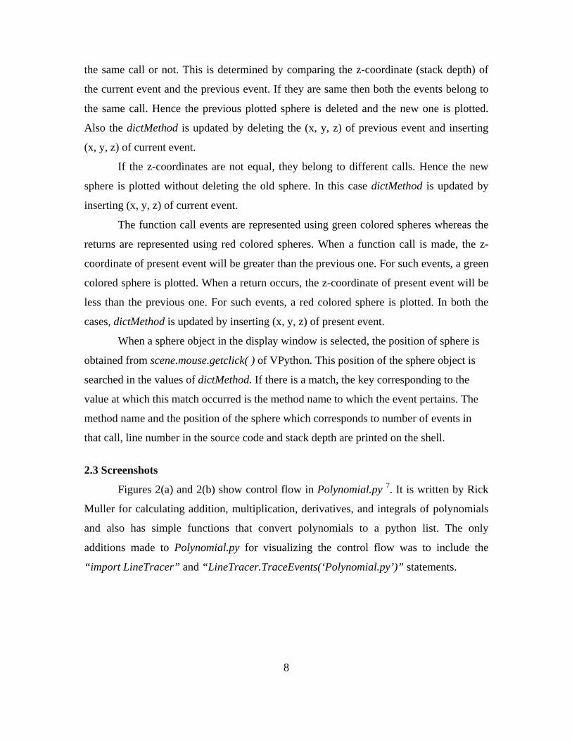
Figure 2(a): control flow in Polynomial.py

The visualization in Figure 2(a) shows axis lines and sphere objects. Each sphere object

corresponds to a line, call or return event. The call events are represented using green

colored spheres and the return events are represented using red colored spheres. The

white colored spheres represent line events. Though a sphere is drawn for each line event,

only the sphere representing final event in a particular call is kept and others are deleted.

10

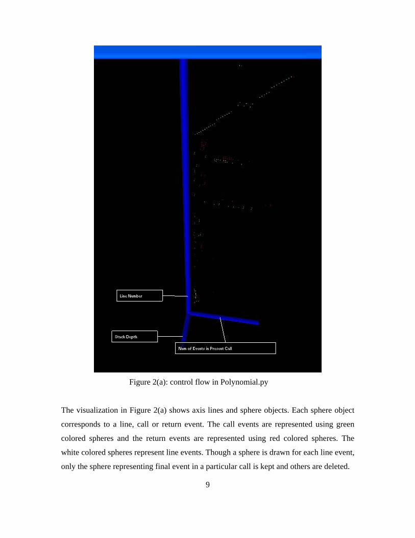
The position of the spheres is based on Number of Events in Current Call, Line

Number and Stack Depth. The z-dimension of each sphere object gives an idea of how

deep the present call is in the program. If the z-cordinate is high, the stack depth is high

and hence the program has to complete many calls before coming to an end.

Figure 2(b): Zoomed and Rotated version of Figure 2(a).

In Figure 2(b), the sphere in cyan color represents the end of the program. Green colored

spheres representing the function calls have a low x-coordinate as expected since this will

be the first event in the call. The function returns represented by red colored spheres have

a high x-coordinate as expected since they are the final events in a call.

11

This first visualization was intended to try and see whether the Profiling and

Tracing hooks provided by the Python Interpreter are helpful. Another goal was to get

familiarized with VPython. I think this tool served a very good practice exercise in terms

of understanding the Profiling and Tracing hooks and also Vpython but nothing

interesting regarding control flow could be seen using it.

3. Second Visualization Tool

One of the problems with the line level visualization is that it has a lot of events to

depict which makes it look complex and less informative. This visualization overcomes

this problem by plotting only the function/method call events in a program. Visualizer.py

represents the functions and classes present in the source program by the sides of a

polygon. The call events are represented by plotting arrows from caller to called

function/method.

There process for obtaining visualization is very simple. It is a single step

process. There is no need to import any modules into user program. The Visualizer.py

should be executed with the name of user program as a command line argument. Other

optional parameters and the method of executing Visualizer is:

python Visualizer.py [-d] [-a] progName [Args]

If the ‘-d’ option is 2; a 2D visualization for the progName is plotted. If it is 3; a 3D

visualization is plotted. By default 3D visualization is plotted. The ‘-a’ flag defines

number of arrows to be shown in the visualization at every instance. The recent ‘a’

number of arrows are shown and the older arrow is deleted. Default value for ‘-a’ is 50.

This ‘-a’ flag is not applicable for 2D visualization.

3.1 Visualizer.py

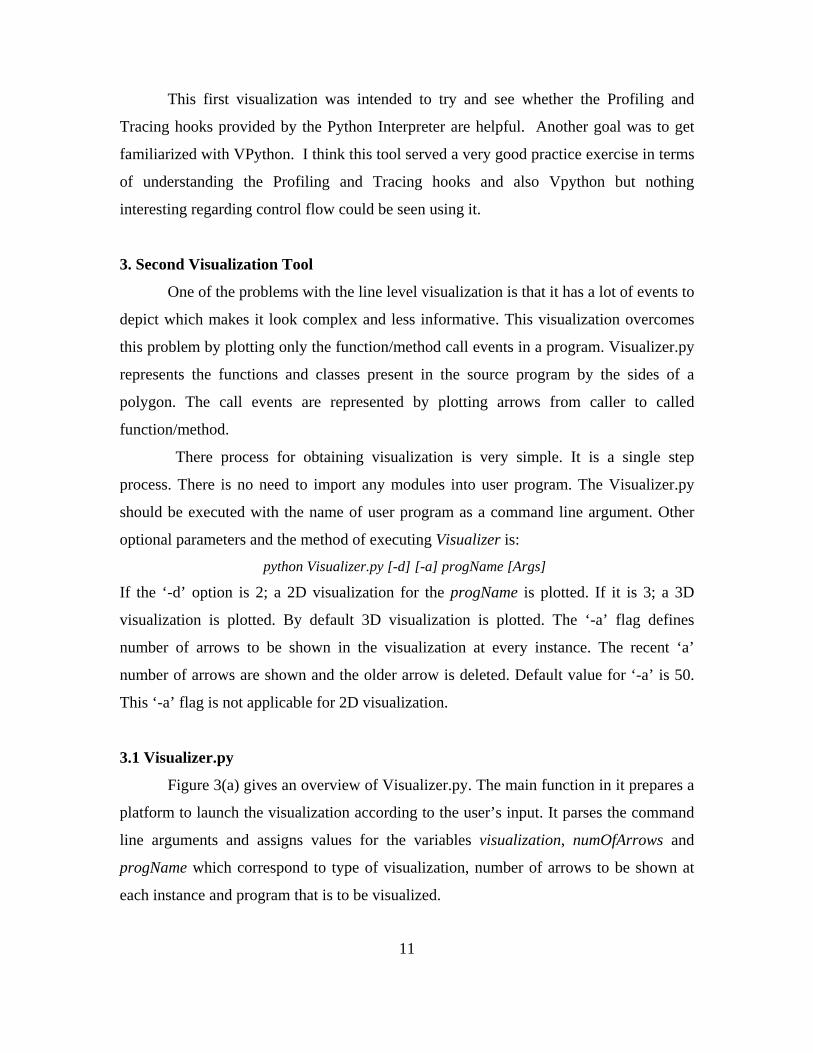
Figure 3(a) gives an overview of Visualizer.py. The main function in it prepares a

platform to launch the visualization according to the user’s input. It parses the command

line arguments and assigns values for the variables visualization, numOfArrows and

progName which correspond to type of visualization, number of arrows to be shown at

each instance and program that is to be visualized.

12

Figure 3(a): Visualizer.py

The log file events.txt is opened in the append mode to write the profiling results.

A profiling function is installed using sys.setprofile(eventTracer). In this visualization,

the sys module’s setprofile function is chosen instead of settrace because the visualization

doesn’t need information about line events.

The user’s program is executed by using Python’s built-in function execfile( )

which takes progName as the parameter. During its execution, the Python Interpreter

calls eventTracer( ) for every call and return event with specific parameters. Required

information for visualizing the control flow such as name of the caller, and called are

extracted and written into log file events.txt. Figure 3(b) describes the algorithm of

eventTracer( ).

execfile(progName)

sys.setprofile(None)

Check if –d flag is 2

execfile(CallGraph2D) execfile(CallGraph)

Yes No

sys.setprofile(eventTracer)

Parse the command line arguments

13

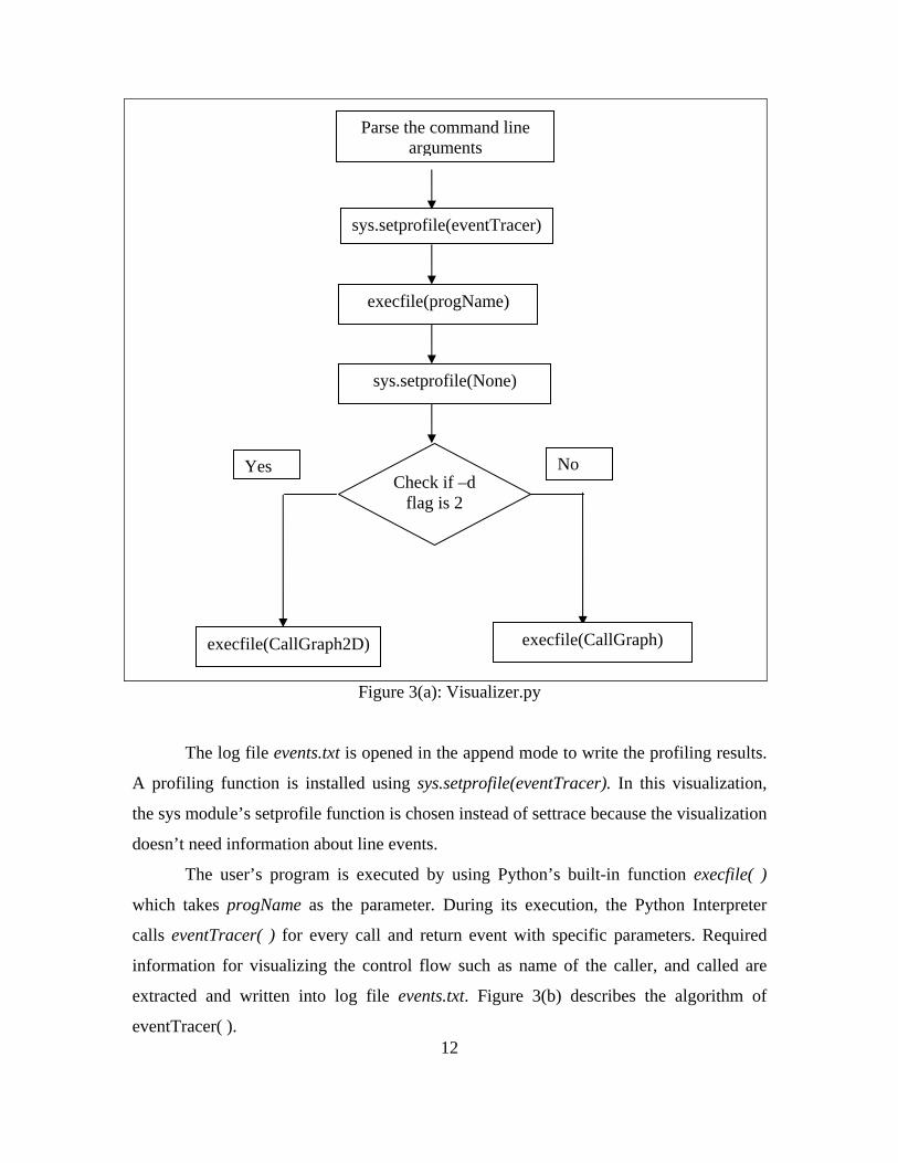
frame.f_code.co_name returns the name of the called function or method. If a

method is called, the name of the class to which this method belongs to is obtained from

frame .f_locals["self"].__class__. __name__.

The name of calling function/method is obtained from frame. f_back.f_code.

co_name 13. Similarly frame. f_back.f_locals["self"].__class__. __name__ returns the

class name to which this method belongs. Appendix A provides more information about

frame and code objects.

def eventTracer ( frame, event, arg) { if (event == “call”){ if called is Method: if caller is Method:

logfile.write (Method, Called Method Name, Class Name, Method, Calling Method Name, Class Name)

else: logfile.write (Method, Called Method Name, Class Name, Function, Function Name)

else: if caller is Method:

logfile.write (Function, Function Name, Method, Calling Method Name, Class Name)

else: logfile.write (Function, Called Function Name, Function, Calling Function Name)

} }

Figure 3(b): eventTracer function

After executing the user’s program, the profiling function is disabled by using

sys.setprofile(None). The 2D or 3D visualization program is invoked depending on the

user’s choice.

3.2 CallGraph.py

The 3D visualization program CallGraph uses the information from events.txt to

plot the visualization. It iterates two times over the log file events.txt. In the first iteration

it finds all the classes, methods and functions in the user program and stores them into

14

dictionary and list objects. In the second iteration it plots the arrows in Control Flow

Visualization window. CallGraph uses an ordered dictionary instead of the ordinary

dictionary object provided by python. It imports odict 8 module written by Nicola Larosa

and Michael Foord which defines the OrderedDict class. The reason for using

OrderedDict is explained later in the second paragraph of section 3.3.2.

CallGraph plots the control flow of a program using arrow and sphere objects.

CallGraph draws an irregular polygon on XY axis with each side representing a function

or Class of the user program. The side representing to a class is further divided to

represent methods. These sub-divisions are colored blue and green alternately to

differentiate the methods in that class.

The length of each side in the polygon is proportional to total number of calls

made and received by the corresponding function or Class. The length of each

subdivision representing a method is proportional to total calls made and received by it

when compared to its Class. Arrows are drawn from the calling function to called

function with tip of the arrow pointing called function.

Figure 4 gives an overview of CallGraph.py. CallGraph creates a control window

and two display windows. The control window shows a slider object with which a user

can control the speed with which the arrows are plotted in the Control Flow Visualization

display window. Appendix B gives a brief description control window, display window

and slider objects. The first display window is the Control Flow Visualization window

where control flow in the user program is plotted. The second display window, Functions

and Classes depicts all the functions and classes present in the user program in the form

of an irregular polygon.

15

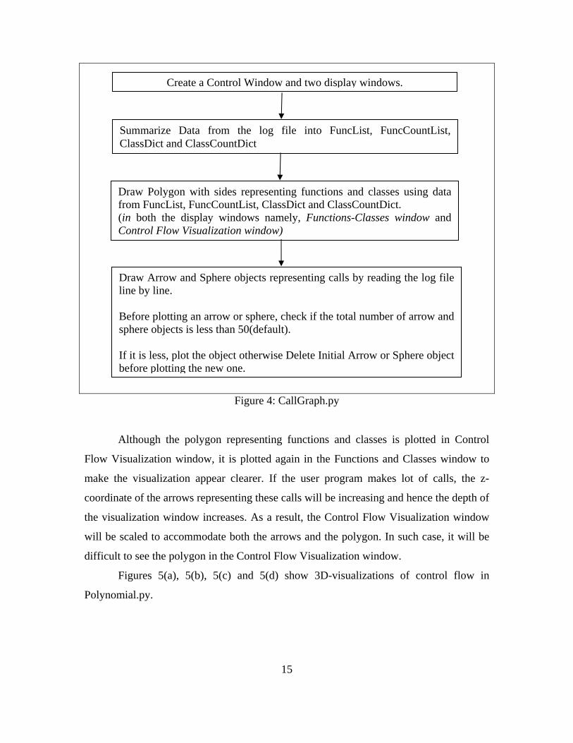
Figure 4: CallGraph.py

Although the polygon representing functions and classes is plotted in Control

Flow Visualization window, it is plotted again in the Functions and Classes window to

make the visualization appear clearer. If the user program makes lot of calls, the z-

coordinate of the arrows representing these calls will be increasing and hence the depth of

the visualization window increases. As a result, the Control Flow Visualization window

will be scaled to accommodate both the arrows and the polygon. In such case, it will be

difficult to see the polygon in the Control Flow Visualization window.

Figures 5(a), 5(b), 5(c) and 5(d) show 3D-visualizations of control flow in

Polynomial.py.

Summarize Data from the log file into FuncList, FuncCountList, ClassDict and ClassCountDict

Draw Polygon with sides representing functions and classes using data from FuncList, FuncCountList, ClassDict and ClassCountDict. (in both the display windows namely, Functions-Classes window and Control Flow Visualization window)

Draw Arrow and Sphere objects representing calls by reading the log file line by line. Before plotting an arrow or sphere, check if the total number of arrow and sphere objects is less than 50(default). If it is less, plot the object otherwise Delete Initial Arrow or Sphere object before plotting the new one.

Create a Control Window and two display windows.

16

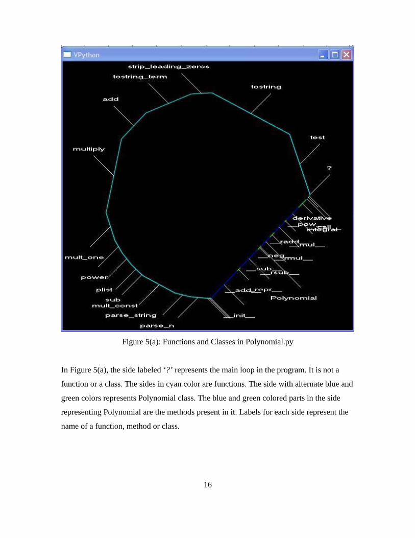
Figure 5(a): Functions and Classes in Polynomial.py

In Figure 5(a), the side labeled ‘?’ represents the main loop in the program. It is not a

function or a class. The sides in cyan color are functions. The side with alternate blue and

green colors represents Polynomial class. The blue and green colored parts in the side

representing Polynomial are the methods present in it. Labels for each side represent the

name of a function, method or class.

17

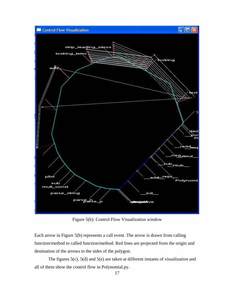
Figure 5(b): Control Flow Visualization window

Each arrow in Figure 5(b) represents a call event. The arrow is drawn from calling

function/method to called function/method. Red lines are projected from the origin and

destination of the arrows to the sides of the polygon.

The figures 5(c), 5(d) and 5(e) are taken at different instants of visualization and

all of them show the control flow in Polynomial.py.

18

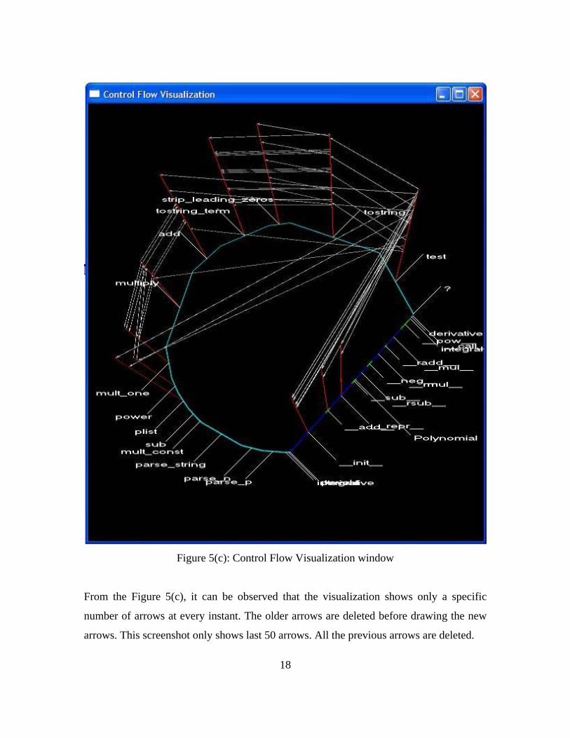
Figure 5(c): Control Flow Visualization window

From the Figure 5(c), it can be observed that the visualization shows only a specific

number of arrows at every instant. The older arrows are deleted before drawing the new

arrows. This screenshot only shows last 50 arrows. All the previous arrows are deleted.

19

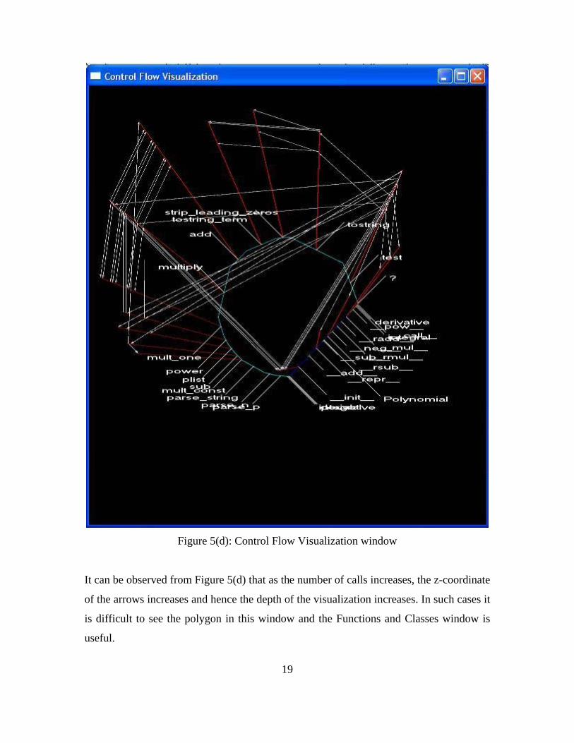
Figure 5(d): Control Flow Visualization window

It can be observed from Figure 5(d) that as the number of calls increases, the z-coordinate

of the arrows increases and hence the depth of the visualization increases. In such cases it

is difficult to see the polygon in this window and the Functions and Classes window is

useful.

20

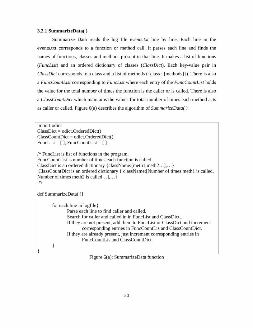
3.2.1 SummarizeData( )

Summarize Data reads the log file events.txt line by line. Each line in the

events.txt corresponds to a function or method call. It parses each line and finds the

names of functions, classes and methods present in that line. It makes a list of functions

(FuncList) and an ordered dictionary of classes (ClassDict). Each key-value pair in

ClassDict corresponds to a class and a list of methods ({class : [methods]}). There is also

a FuncCountList corresponding to FuncList where each entry of the FuncCountList holds

the value for the total number of times the function is the caller or is called. There is also

a ClassCountDict which maintains the values for total number of times each method acts

as caller or called. Figure 6(a) describes the algorithm of SummarizeData( ).

import odict ClassDict = odict.OrderedDict() ClassCountDict = odict.OrderedDict() FuncList = [ ], FuncCountList = [ ] /* FuncList is list of functions in the program. FuncCountList is number of times each function is called. ClassDict is an ordered dictionary {className:[meth1,meth2…],…}. ClassCountDict is an ordered dictionary { className:[Number of times meth1 is called, Number of times meth2 is called…],…} */ def SummarizeData( ){ for each line in logfile{ Parse each line to find caller and called. Search for caller and called in in FuncList and ClassDict,. If they are not present, add them to FuncList or ClassDict and increment corresponding entries in FuncCountLis and ClassCountDict. If they are already present, just increment corresponding entries in FuncCountLis and ClassCountDict. } }

Figure 6(a): SummarizeData function

21

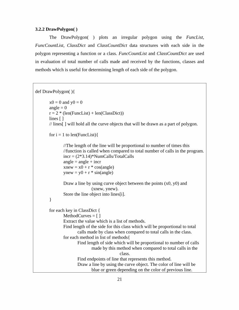
3.2.2 DrawPolygon( )

The DrawPolygon( ) plots an irregular polygon using the FuncList,

FuncCountList, ClassDict and ClassCountDict data structures with each side in the

polygon representing a function or a class. FuncCountList and ClassCountDict are used

in evaluation of total number of calls made and received by the functions, classes and

methods which is useful for determining length of each side of the polygon.

def DrawPolygon( ){ x0 = 0 and y0 = 0 angle = 0

r = 2 * (len(FuncList) + len(ClassDict)) lines [ ] // lines[ ] will hold all the curve objects that will be drawn as a part of polygon.

for i = 1 to len(FuncList){

//The length of the line will be proportional to number of times this //function is called when compared to total number of calls in the program. incr = (2*3.14)*NumCalls/TotalCalls

angle = angle + incr xnew = x0 + r * cos(angle) ynew = y0 + r * sin(angle) Draw a line by using curve object between the points (x0, y0) and

(xnew, ynew). Store the line object into lines[i]. } for each key in ClassDict { MethodCurves = [ ] Extract the value which is a list of methods. Find length of the side for this class which will be proportional to total calls made by class when compared to total calls in the class. for each method in list of methods{ Find length of side which will be proportional to number of calls made by this method when compared to total calls in the class. Find endpoints of line that represents this method. Draw a line by using the curve object. The color of line will be blue or green depending on the color of previous line.

22

Append this curve object into MethodCurves[ ] } Append MethodCurves list to lines[ ] } }

Figure 6(b): DrawPolygon function

The algorithm in Figure 6(b) describes the DrawPolygon( ). The polygon

representing functions and classes is drawn in anticlockwise direction with origin as

center and radius equal to twice the number of sides. The first part of polygon has

functions and the remaining part has classes. The polygon itself shows part of control

flow. The order of the sides in the polygon is based on the order in which they are first

called. Thus the sides representing functions are in the order of first call and also the

sides representing classes are in the order of first call. But as a whole the functions and

classes are not in the order of first call. OrderedDict 8 object of odict module is used

instead of the dictionary object to maintain the order of first called classes.

DrawPolygon uses Vpython’s curve object to draw straight lines to form a

polygon. VPython doesn’t have a line object. The list data structure, lines[ ] is used to

store all the curve objects of the polygon.

3.2.3 DrawArrows( )

The DrawArrows function plots arrows and spheres from the caller to called

function / method. The algorithm in Figure 6(c) describes DrawArrows( ) which reads the

log file events.txt line by line until the end of file. It parses each line to find the caller and

called. FuncList and ClassDict are searched to find the indexes of caller and called. The

list lines[] is searched with these indexes to locate the sides of polygon which correspond

to the caller and called. The midpoints for such sides are calculated and are termed as

(StartLineMidY, StartLineMidY) and (DestLineMidX, DestLineMidY) respectively. For

each line read from the events.txt, a variable zcoord is incremented by 0.5 which forms

the Z-Coordinate for these midpoints.

23

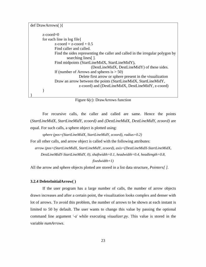
def DrawArrows( ){

z-coord=0 for each line in log file{ z-coord = z-coord + 0.5 Find caller and called. Find the sides representing the caller and called in the irregular polygon by searching lines[ ]. Find midpoints (StartLineMidX, StartLineMidY), (DestLineMidX, DestLineMidY) of these sides. If (number of Arrows and spheres is > 50) Delete first arrow or sphere present in the visualization Draw an arrow between the points (StartLineMidX, StartLineMidY, z-coord) and (DestLineMidX, DestLineMidY, z-coord) } }

Figure 6(c): DrawArrows function

For recursive calls, the caller and called are same. Hence the points

(StartLineMidX, StartLineMidY, zcoord) and (DestLineMidX, DestLineMidY, zcoord) are

equal. For such calls, a sphere object is plotted using:

sphere (pos=(StartLineMidX, StartLineMidY, zcoord), radius=0.2)

For all other calls, and arrow object is called with the following attributes:

arrow (pos=(StartLineMidX, StartLineMidY, zcoord), axis=(DestLineMidX-StartLineMidX,

DestLineMidY-StartLineMidY, 0), shaftwidth=0.1, headwidth=0.4, headlength=0.8,

fixedwidth=1)

All the arrow and sphere objects plotted are stored in a list data structure, Pointers[ ].

3.2.4 DeleteInitialArrow( )

If the user program has a large number of calls, the number of arrow objects

drawn increases and after a certain point, the visualization looks complex and denser with

lot of arrows. To avoid this problem, the number of arrows to be shown at each instant is

limited to 50 by default. The user wants to change this value by passing the optional

command line argument '-a' while executing visualizer.py. This value is stored in the

variable numArrows.

24

For every line read from the log file events.txt (i.e for every call event), the

variable counter is incremented. Before drawing an arrow or a sphere object, the counter

is compared with numArrows (default 50). If the counter is greater than numArrows,

Pointers[arrowIndex] is deleted by my making its attribute visible=0. The variable

arrowIndex is initialized to 0 at the beginning of DrawArrows and is incremented after

deletion of an object from Pointers. Thus arrowIndex is used to keep track of the first

arrow present at every instance in the visualization.

3.3 CallGraph2D.py

The CallGraph2D program plots a 2D-visualization for the control flow in the

user program. It creates two display windows. The first window, Control Flow

Visualization, shows the control flow as a 2D plot and the second window, Functions and

Classes, shows an irregular polygon representing functions and classes in the program.

There is no control window in this visualization.

The Z-dimension is neglected in this 2D-Visualization. All the arrow and sphere

objects representing calls are in the XY plane. Before plotting an arrow, CallGraph2D

checks whether an arrow is already present between the specific points. If there is an

arrow, the older arrow is deleted and a new arrow is drawn with its shaftwidth increased

by 0.1. In the case of recursion, the old sphere object is deleted and a new sphere is

plotted at the same point but with radius increased by 0.1.

25

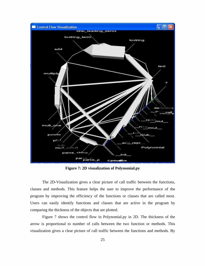
Figure 7: 2D visualization of Polynomial.py

The 2D-Visualization gives a clear picture of call traffic between the functions,

classes and methods. This feature helps the user to improve the performance of the

program by improving the efficiency of the functions or classes that are called most.

Users can easily identify functions and classes that are active in the program by

comparing the thickness of the objects that are plotted.

Figure 7 shows the control flow in Polynomial.py in 2D. The thickness of the

arrow is proportional to number of calls between the two function or methods. This

visualization gives a clear picture of call traffic between the functions and methods. By

26

improving the efficiency of code in mostly called functions or methods, the performance

of the program can be improved.

4. Interesting Screenshots

This section shows some interesting screen shots obtained by executing

Visualizer.py on different programs. Each of these visualizations has some interesting

information associated with it. Brief introduction of each program is followed by some

interesting screen shots and information.

4.1 Dataenc.py 9 (cited in 10)

This module can be used for combining data using a ‘binary interleave’ where

two pieces of data are woven together a bit at a time. The resulting binary string can be

converted into an ASCII string using a table encoding. This module provides a simple

mechanism for secure, time limited, logins when writing CGIs. This program is written

by Michael Foord.

27

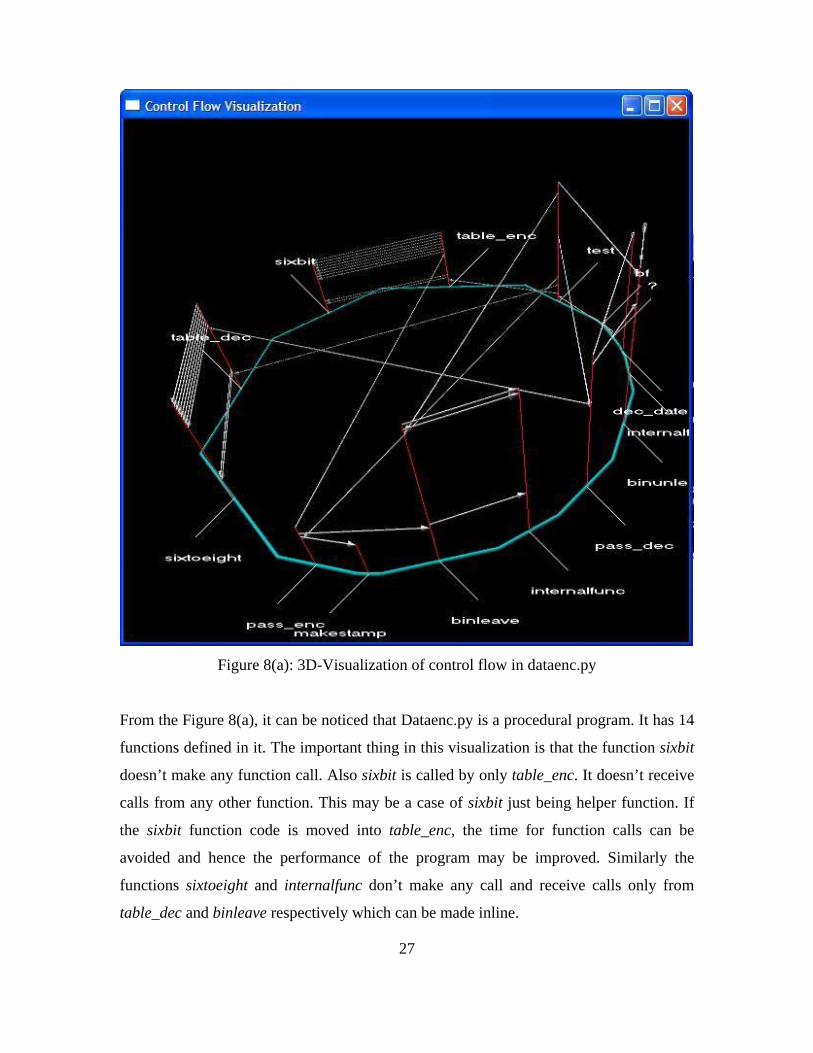
Figure 8(a): 3D-Visualization of control flow in dataenc.py

From the Figure 8(a), it can be noticed that Dataenc.py is a procedural program. It has 14

functions defined in it. The important thing in this visualization is that the function sixbit

doesn’t make any function call. Also sixbit is called by only table_enc. It doesn’t receive

calls from any other function. This may be a case of sixbit just being helper function. If

the sixbit function code is moved into table_enc, the time for function calls can be

avoided and hence the performance of the program may be improved. Similarly the

functions sixtoeight and internalfunc don’t make any call and receive calls only from

table_dec and binleave respectively which can be made inline.

28

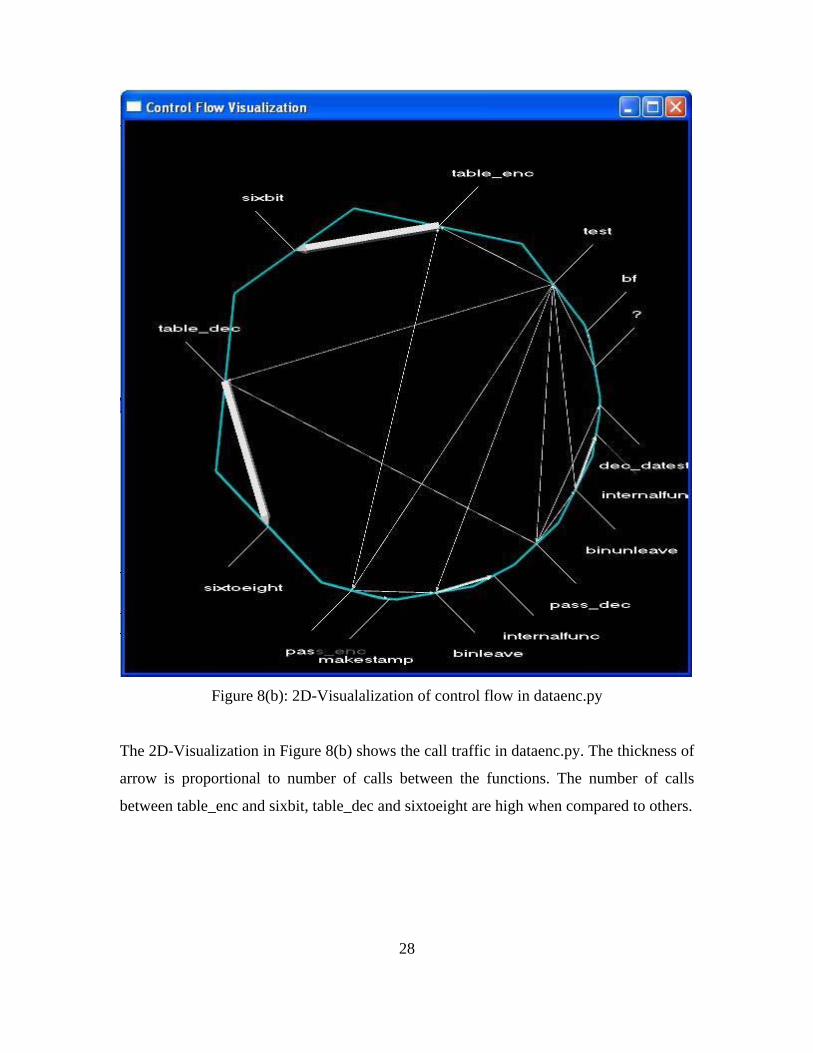
Figure 8(b): 2D-Visualalization of control flow in dataenc.py

The 2D-Visualization in Figure 8(b) shows the call traffic in dataenc.py. The thickness of

arrow is proportional to number of calls between the functions. The number of calls

between table_enc and sixbit, table_dec and sixtoeight are high when compared to others.

29

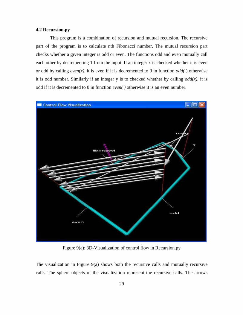
4.2 Recursion.py

This program is a combination of recursion and mutual recursion. The recursive

part of the program is to calculate nth Fibonacci number. The mutual recursion part

checks whether a given integer is odd or even. The functions odd and even mutually call

each other by decrementing 1 from the input. If an integer x is checked whether it is even

or odd by calling even(x), it is even if it is decremented to 0 in function odd( ) otherwise

it is odd number. Similarly if an integer y is to checked whether by calling odd(x), it is

odd if it is decremented to 0 in function even( ) otherwise it is an even number.

Figure 9(a): 3D-Visualization of control flow in Recursion.py

The visualization in Figure 9(a) shows both the recursive calls and mutually recursive

calls. The sphere objects of the visualization represent the recursive calls. The arrows

30

from odd to even and even to odd represent the mutual recursive calls. This program is

taken to show how the recursive calls are handled by this visualization.

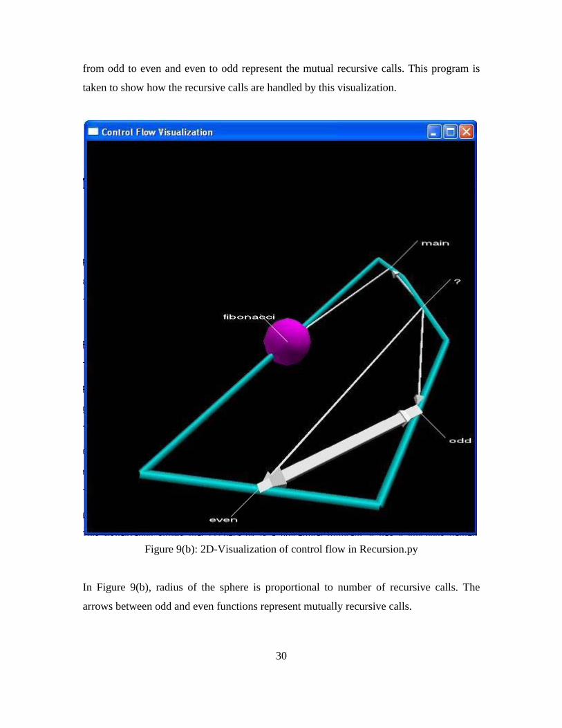
Figure 9(b): 2D-Visualization of control flow in Recursion.py

In Figure 9(b), radius of the sphere is proportional to number of recursive calls. The

arrows between odd and even functions represent mutually recursive calls.

31

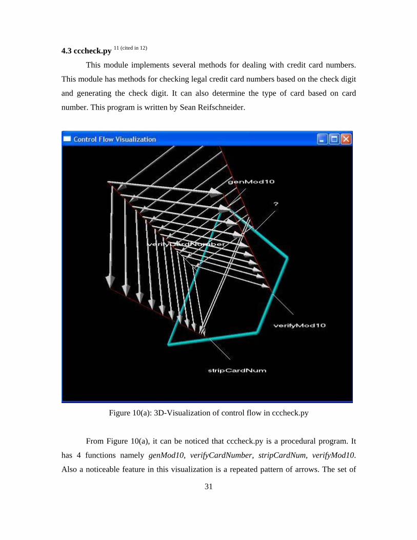
4.3 cccheck.py 11 (cited in 12)

This module implements several methods for dealing with credit card numbers.

This module has methods for checking legal credit card numbers based on the check digit

and generating the check digit. It can also determine the type of card based on card

number. This program is written by Sean Reifschneider.

Figure 10(a): 3D-Visualization of control flow in cccheck.py

From Figure 10(a), it can be noticed that cccheck.py is a procedural program. It

has 4 functions namely genMod10, verifyCardNumber, stripCardNum, verifyMod10.

Also a noticeable feature in this visualization is a repeated pattern of arrows. The set of

32

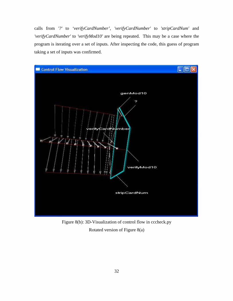
calls from '?' to ‘verifyCardNumber’, 'verifyCardNumber' to 'stripCardNum' and

'verifyCardNumber' to 'verifyMod10' are being repeated. This may be a case where the

program is iterating over a set of inputs. After inspecting the code, this guess of program

taking a set of inputs was confirmed.

Figure 8(b): 3D-Visualization of control flow in cccheck.py

Rotated version of Figure 8(a)

33

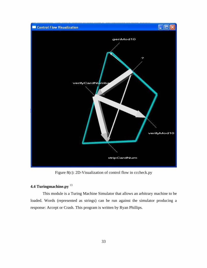
Figure 8(c): 2D-Visualization of control flow in cccheck.py

4.4 Turingmachine.py 13

This module is a Turing Machine Simulator that allows an arbitrary machine to be

loaded. Words (represented as strings) can be run against the simulator producing a

response: Accept or Crash. This program is written by Ryan Phillips.

34

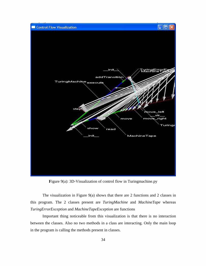
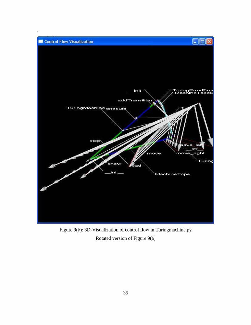
Figure 9(a): 3D-Visualization of control flow in Turingmachine.py

The visualization in Figure 9(a) shows that there are 2 functions and 2 classes in

this program. The 2 classes present are TuringMachine and MachineTape whereas

TuringErrorException and MachineTapeException are functions

Important thing noticeable from this visualization is that there is no interaction

between the classes. Also no two methods in a class are interacting. Only the main loop

in the program is calling the methods present in classes.

35

.

Figure 9(b): 3D-Visualization of control flow in Turingmachine.py

Rotated version of Figure 9(a)

36

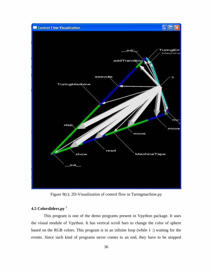
Figure 9(c): 2D-Visualization of control flow in Turingmachine.py

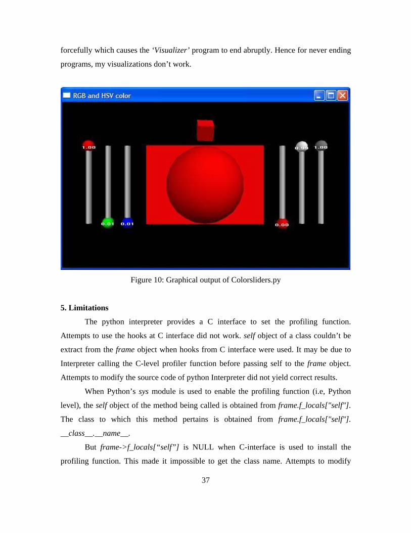
4.5 Colorsliders.py 5

This program is one of the demo programs present in Vpython package. It uses

the visual module of Vpython. It has vertical scroll bars to change the color of sphere

based on the RGB colors. This program is in an infinite loop (while 1 :) waiting for the

events. Since such kind of programs never comes to an end, they have to be stopped

37

forcefully which causes the ‘Visualizer’ program to end abruptly. Hence for never ending

programs, my visualizations don’t work.

Figure 10: Graphical output of Colorsliders.py

5. Limitations

The python interpreter provides a C interface to set the profiling function.

Attempts to use the hooks at C interface did not work. self object of a class couldn’t be

extract from the frame object when hooks from C interface were used. It may be due to

Interpreter calling the C-level profiler function before passing self to the frame object.

Attempts to modify the source code of python Interpreter did not yield correct results.

When Python’s sys module is used to enable the profiling function (i.e, Python

level), the self object of the method being called is obtained from frame.f_locals["self"].

The class to which this method pertains is obtained from frame.f_locals["self"].

__class__.__name__.

But frame->f_locals[“self”] is NULL when C-interface is used to install the

profiling function. This made it impossible to get the class name. Attempts to modify

38

Interpreter code in Python2.4.1/Python/ceval.c (interpreter main loop) did not work.

6. Conclusion

This Control Flow Visualization tool plots the call events between functions,

classes and methods in a program. It gives a clear and often interesting picture of the

number of functions, methods and classes present in a python program. This gives the

user an overview of the program. The functions, classes and methods receiving and

making more calls are represented by longer sides of the irregular polygon. This helps in

identifying functions, classes and methods that are active in the program.

The 3D-Visualization depicts the control flow in a program at coarse-level

granularity. Control flow between functions, classes and methods is clearly shown by the

3D visualization with arrow and sphere objects using the z-coordinate. The 3D

visualization also provides a slider to adjust the speed of visualization. Thus the user can

concentrate more at his points of interest by moving the scroll bar to left or neglect by

moving it to right. Recursive calls can be identified easily which are represented by using

sphere objects.

The 2D-Visualization gives a clear picture of call traffic between the functions,

classes and methods. This can help in improving the performance of the program by

increasing the efficiency of the code in specific functions, classes and methods.

While the tools developed in this project do not specifically find bugs or tune the

performance of programs, they do appear to be useful in helping programmers understand

programs, which may aid them in debugging or performance tuning tasks.

7. Acknowledgements

I thank my advisor, Dr. Clinton Jeffery, for his valuable suggestions and

guidance through out the project. I would also like to thank my friend, Mahesh Chittur,

for helping me in the installation of VPython on Suse and Fedora systems.

References

[1] Jeffery CL. 1999. Program Monitoring and Visualization : An Exploratory Approach.

New York: Springer-Verlag New York. 209 p.

39

[2] [Anonymous]. 2005. Python. Available from: http://www.python.org.

Accessed 2005 Jan.

[3] Rossum G. 2005 Sept 28. sys -- System-specific parameters and functions.

Available from: http://docs.python.org/lib/module-sys.html. Accessed 2005 Feb.

[4] Rossum G. 2005 Sept 28. Profiling and Tracing. Python/C API Reference Manual.

Available from: http://docs.python.org/api/profiling.html. Accessed 2005 Feb.

[5] [Anonymous]. 2005. VPython overview. Available from:

http://vpython.org/VisualOverview.html. Accessed 2005 Feb.

[6] Rossum G. 2005 Sept 28. Extending Python with C or C++. Available from:

http://docs.python.org/ext/intro.html. Accessed 2005 Feb.

[7] [ASPN] ActiveState Programmer Network. 2005. Manipulate simple polynomials in

Python. Available from:

http://aspn.activstate.com/ASPN/Cookbook/Python/Recipe/362193. Accessed

2005 April.

[8] [Anonymous]. 2005 Sept 12. The odict Module. An Ordered Dictionary. Available

from: http://www.voidspace.org.uk/python/odict.html. Accessed 2005 Sept.

[9] [Anonymous]. 2005 Sept. dataenc. The Voidspace Python Modules. Available from:

http://www.voidspace.org.uk/python/modules.shtml#dataenc. Accessed 2005 Oct.

[10] [Anonymous]. 2005 Aug. Dataenc 1.1.4. Vaults of Paranassus : Python Resources.

Available from: http://py.vaults.ca/apyllo.py?find=dataenc. Accessed 2005 Oct.

[11] [Anonymous]. Cccheck-1.0.0. Available from:

ftp://ftp.tummy.com/pub/tummy/cccheck/. Accessed 2005 Oct.

[12] [Anonymous]. 2005 Aug. Credit Card Number Module. Vaults of Paranassus:

Python Resources. Available from: http://py.vaults.ca/apyllo.py?find=credit+card.

Accessed 2005 Oct.

[13] [ASPN] ActiveState Programmer Network. 2005. Turing Machine Simulator.

Available from:

http://aspn.activestate.com/ASPN/Cookbook/Python/Recipe/252486. Accessed

2005 Oct.

40

APPENDIX A

Tracing Hooks provided by the C interface of Python

Python interpreter provides profiling and execution tracing facilities which are

useful for debugging and coverage analysis tools 4. Python provides a C interface to set

tracing and profiling functions which receive the information useful for program

visualization especially the control flow visualization.

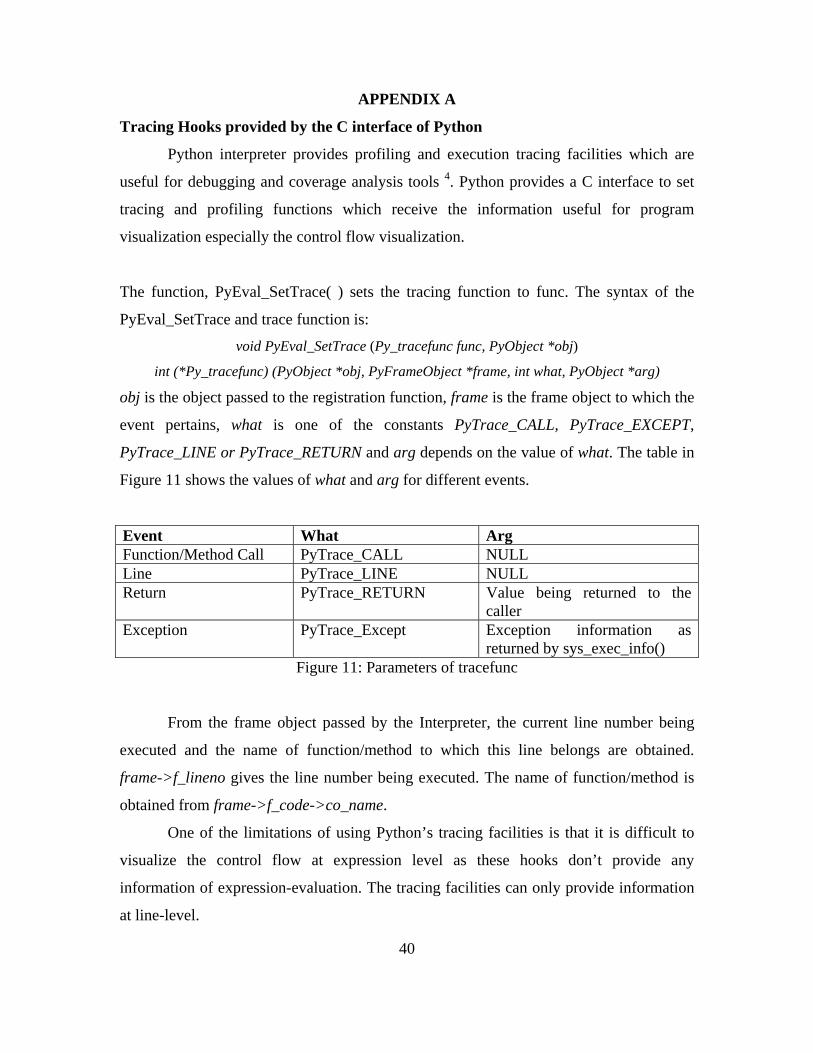
The function, PyEval_SetTrace( ) sets the tracing function to func. The syntax of the

PyEval_SetTrace and trace function is:

void PyEval_SetTrace (Py_tracefunc func, PyObject *obj) int (*Py_tracefunc) (PyObject *obj, PyFrameObject *frame, int what, PyObject *arg)

obj is the object passed to the registration function, frame is the frame object to which the

event pertains, what is one of the constants PyTrace_CALL, PyTrace_EXCEPT,

PyTrace_LINE or PyTrace_RETURN and arg depends on the value of what. The table in

Figure 11 shows the values of what and arg for different events.

Event What Arg Function/Method Call PyTrace_CALL NULL Line PyTrace_LINE NULL Return PyTrace_RETURN Value being returned to the

caller Exception PyTrace_Except Exception information as

returned by sys_exec_info() Figure 11: Parameters of tracefunc

From the frame object passed by the Interpreter, the current line number being

executed and the name of function/method to which this line belongs are obtained.

frame->f_lineno gives the line number being executed. The name of function/method is

obtained from frame->f_code->co_name.

One of the limitations of using Python’s tracing facilities is that it is difficult to

visualize the control flow at expression level as these hooks don’t provide any

information of expression-evaluation. The tracing facilities can only provide information

at line-level.

41

A detailed description of profiling and tracing facilities provided by Python’s C

interface is available at http://docs.python.org/api/profiling.html.

Profiling Facilities provided by sys module of Python

The sys module in python allows installing a profiling function using setprofile

function. The interpreter calls the profiler function for every call and return event.

sys.setprofile(funcName) sets funcName as profiling function. Python Interpreter calls

the funcName with frame, event and arg as parameters. The syntax of profiling function

is:

def funcName (frame, event, arg)

frame corresponds to the frame object to which the event pertains. event will be a call or

a return. arg depends on the event. If the event is a call, arg is NULL; if the event is a

return, arg is the value returned to the caller.

The sys module allows installing tracing function also. sys.settrace(funcName)

sets funcName as tracing function. The only difference between tracing and profiler

functions is that the Interpreter calls the tracing function for every executed line of code.

More information on sys module can be obtained from the Python documentation

available at http://docs.python.org/lib/module-sys.html.

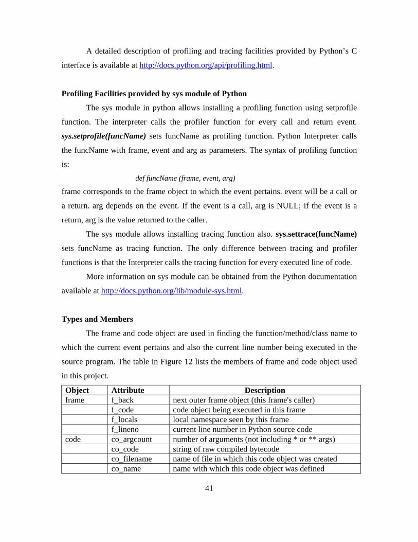
Types and Members

The frame and code object are used in finding the function/method/class name to

which the current event pertains and also the current line number being executed in the

source program. The table in Figure 12 lists the members of frame and code object used

in this project.

Object Attribute Description frame f_back next outer frame object (this frame's caller) f_code code object being executed in this frame f_locals local namespace seen by this frame f_lineno current line number in Python source code code co_argcount number of arguments (not including * or ** args) co_code string of raw compiled bytecode co_filename name of file in which this code object was created co_name name with which this code object was defined

42

A detailed list of Python’s Types and Members is provided in Python’s documentation at

http://www.python.org/doc/2.2.3/lib/inspect-types.html

APPENDIX B

Display window

display( ) creates a display window with the specified attributes, makes it the selected

display, and returns it.

scene2 = display (title = 'Graph of position', x = 0, y = 0, width=600, height=200, center = (5, 0,

0), background = (0, 1, 1))

x, y - Position of the window on the screen (pixels from upper left)

width, height - Width and height of the display area in pixels.

title - Text in the control window's title bar.

center - Location at which the camera continually looks, even as the user rotates the

position of the camera.

background Set color to be used to fill the display window; default is black.

Controls window

controls( ) Creates a controls window with the specified attributes, and returns it. After

creating a controls window, objects such as button, slider, toggle and menu can be

created in it.

c = controls (title='Controlling the Scene', x=0, y=400, width=300, height=300, range=50)

x, y - Position of the window on the screen (pixels from upper left)

width, height - Width and height of the display area in pixels.

title - Text in the control window's title bar.

range - The extent of the region of interest away from the center along each axis. The

default is 100. The center of a controls window is always (0, 0).

Sphere

The syntax of the sphere object is:

sphere (pos=(x, y, z), radius=r)

pos is the center and radius is radius of the sphere.

43

Arrow

The syntax of arrow object is:

arrow (pos=(x1, y1, z1), axis=(x2, y2, z2), shaftwidth=sw, headwidth=hw, headlength=hl,

fixedlength=1)

The parameters headwidth, headlength and fixedwidth are optional.

By default, shaftwidth = 0.1*(length of arrow),

headwidth = 2*shaftwidth

headlength = 3*shaftwidth.

If you prefer that shaftwidth and headwidth not change as the arrow gets very short or

very long, set fixedwidth=1.

Curve

The syntax of curve Object is:

curve (pos = [(x1,y1), (x2,y2)], radius=r, color = clr)

where pos[ ] is Array of position of points in the curve,

radius is Radius of cross-section of curve and

color is Color of points in the curve.

A detailed description of the objects in VPython is available at

http://vpython.org/webdoc/visual/index.html.