Control Chart for Waiting Time in System of (M/M/1

International Journal of Computer Applications (0975 – 8887)

Volume 63– No.3, February 2013

1

Control Chart for Waiting Time in System of

(M/M/1): (∞/FCFS) Queuing Model

T.Poongodi

Assistant Professor (SG),

Faculty of Engineering,

Avinashilingam Institute for Home Science and

Higher Education for Women

Coimbatore, India

S.Muthulakshmi, PhD. Professor,

Faculty of Science,

Avinashilingam Institute for Home Science and

Higher Education for Women

Coimbatore, India

ABSTRACT

Queue is a very volatile situation which always cause

unnecessary delay and reduce the service effectiveness of

establishments or service industries. Long queues may create

negative effects like wasting of man power, unnecessary

congestion which leads to suffocation; even develop

complications to customers and also to the establishments.

This necessitates the study of waiting time of the customers

and the facility. Control chart technique may be applied to

analyze the waiting time of the customers in the system to

improve the services and the effective performance of

concerns. Control chart constructed for random variable W,

the time spent in the system, provides the control limits for W.

The prior idea about the expected waiting time, maximum

waiting time and minimum waiting time from the parameters

of the constructed chart makes effective use of time and

guarantees customer’s satisfaction. Keeping this in view, the

construction of control charts for waiting time is proposed for

M /M /1queueing model.

Keywords

Waiting time, Control limits, Poisson arrival and Exponential

service.

1. INTRODUCTION Every manufacturing organization is concerned with the

quality of its product. Stiff competition in the national and

international level and customers’ awareness require

production of quality goods and services for survival and

growth of the company. The most essential ingredient

required to meet this ever growing competition is quality. This

warrants every manufacturing organization to be concerned

with the quality of its product. Quality is to be planned,

improved and monitored continuously.

Shewhart developed control chart techniques based on data of

one or several quality related characteristics of the product or

service to identify whether a production process or service

having goods of set quality standards. Montgomery [2]

proposed a number of applications of control charts in

assuring quality in manufacturing industries.

Shore [3] developed control chart for random queue length, N

of M /M /1queueing model by considering the first three

moments. Khaparde and Dhabe [4] constructed N1, Shewhart

control chart and N2, the control chart using method of

weighted variance for random queue length N for

M/M/1queueing model. With reference to individuals sorting

for facilities the time spent is more influential than the number

in the queueing system. Thus the analysis of time spent in the

system by the control chart provides improvement of the

performance of the system and hence customer satisfaction. In

this paper, an attempt is made to construct Shewhart control

chart for waiting time, W of M/M/1 queueing model. This

model finds applications in a number of fields like assembly

and repairing of machines, aircrafts, ATM facility of banks

etc. where the system is having a single server.

2. M/M/1 MODEL DESCRIPTION

M/M/1 model has single server, Poisson input, exponential

service time and infinite capacity with First Come First Serve

(FCFS) queue discipline. Let λ be the mean arrival rate and µ

be the average service rate.

2.1 Steady state equations

The steady state equations of this model are by [1].

Let

Pn(t) = Probability that there are n customers in the system

(waiting and in service) at time t.

P0(t+Δt) = P0(t) (1 - λΔt) + P1(t) µ Δt + o(Δt )

Pn(t+Δt) = Pn(t) (1-(λ+µ)Δt) + Pn–1(t)λΔt + Pn+1(t)µΔt + o(Δt),

n ≥ 1 (1)

Equation (1) gives

P0′ (t) = - λ P0(t) + µ P1(t)

Pn′ (t) = - (λ + µ)Pn(t) + λPn – 1(t) + µP n+1(t), n ≥ 1 (2)

The steady state equations corresponding to (2) are

0 = - λ P0 + µ P1

0 = - ( λ+µ)Pn+ λPn–1+ µPn+1, n ≥ 1 (3)

Let ρ = μ

λ be the traffic intensity. Equation (3) yields

P0 = (1-ρ)

Pn= (1-ρ) ρn (4)

2.2 Performance measures

(i) E (Ls) = Average number of customers in the system

= n

0n

P n



2

= ρ)(1

ρ

(5)

(ii) E (Lq) = Average number of customers in the queue

= n

1n

P 1)-(n

= ρ)(1

ρ2

(6)

(iii) E (Ws) = Average waiting time of a customer in the

system

=ρ)μ(1

1

(7)

(iv) E (Wq) = Average waiting time of a customer in the queue

= ρ)μ(1

ρ

(8)

Let W denote the waiting time of a customer in the system

which includes both the waiting time and the service time.

The pdf of the random variable W is given by [5]

f (w) = (µ -λ) e- (μ-λ) w, w > 0

which is an exponential distribution with parameter (µ -λ) .

Mean E (W) =)(

1

and variance V (W) =

2)(

1

3. CONTROL CHART FOR WAITING

TIME, W Shewhart type control charts are constructed by

approximating the statistic under consideration by a normal

distribution. The parameters of the control chart are given by

UCL = E(W) + 3 V(W) (9)

CL = E(W)

LCL = E(W) - 3 )V(W

For M /M /1queueing model the parameters of the control

chart for waiting time of the customer in the system are given

by

UCL = )(

4

CL = )(

1

LCL = )(

2

4. NUMERICAL ANALYSIS

Assessment of waiting time in the system by means of control

chart is carried out with numerical illustrations for certain

selected values of λ and µ. Table.1 gives the parameters of the

control chart for various values of the arrival rate λ and a

constant service rate µ = 6.

Table.1 Parameters of control chart with constant service

rate

λ µ ρ CL UCL LCL

1.00 6 0.1667 0.2000 0.8000 -0.4000

1.50 6 0.2500 0.2222 0.8889 -0.4444

2.00 6 0.3333 0.2500 1.0000 -0.5000

2.50 6 0.4167 0.2857 1.1429 -0.5714

3.00 6 0.5000 0.3333 1.3333 -0.6667

3.50 6 0.5833 0.4000 1.6000 -0.8000

4.00 6 0.6667 0.5000 2.0000 -1.0000

4.50 6 0.7500 0.6667 2.6667 -1.3333

5.00 6 0.8333 1.0000 4.0000 -2.0000

5.50 6 0.9167 2.0000 8.0000 -4.0000

From the calculated values of parameters, it is clear that the

increase in arrival rate with constant service rate increases the

average waiting time and the expected upper limit of waiting

time.Table.2 gives the parameters of the control chart for a

constant arrival rate λ = 2 and various values of service rate µ.

Table.2 Parameters of control chart with constant arrival

rate

λ µ ρ CL UCL LCL

2 2.50 0.8000 2.0000 8.0000 -4.0000

2 3.00 0.6667 1.0000 4.0000 -2.0000

2 3.50 0.5714 0.6667 2.6667 -1.3333

2 4.00 0.5000 0.5000 2.0000 -1.0000

2 4.50 0.4444 0.4000 1.6000 -0.8000

2 5.00 0.4000 0.3333 1.3333 -0.6667

2 5.50 0.3636 0.2857 1.1429 -0.5714

2 6.00 0.3333 0.2500 1.0000 -0.5000

From the above table it is seen that if the service rate

increases, the average waiting time and the expected upper

control limit of waiting time decrease for a constant arrival

rate. LCL values in both the cases are considered as 0, since

the values are negative.



3

5. APPLICATION

As an application of the above theoretical calculations, a real

situation, relating to a grocery shop is considered.

A grocery shop has a single server for billing which starts at

8.00 a.m. An arrival moves immediately into the service

facility if it is empty. On the other hand, if the server is busy,

the arrival will wait in the queue. Customers are served on

first come first served basis. Observed inter arrival time and

service time of 200 customers in the system is given in

Table.3. In this table customers, arrival time (min.), inter-

arrival time, starting time of service, service time (min.),

ending time of service and customer’s waiting time in system

(min.) are given in columns I,II,III,IV,V,VI and VII

respectively. Control charts are constructed using the

theoretical formula and also estimated values of observed

data.

From Table.3 the average inter arrival time is 2.755 min. and

the average service time is 2.59 min. Arrival rate λ = 21.78

customers/hr. and service rate µ = 22.90 customers/hr. Using

(9) the parameters of the control chart are calculated as CL =

43.3 min., UCL = 173.2 min. and LCL = 0. The estimated

parameters of the control chart for waiting time are calculated

as

CL = E (Ŵ) = 6.16 min

UCL = E (Ŵ) + 3 )ˆ(WV = 19.84 min

LCL = E (Ŵ) - 3 )ˆ(WV = 0,

based on sample observations.

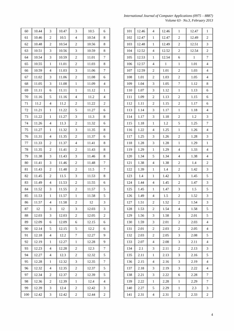
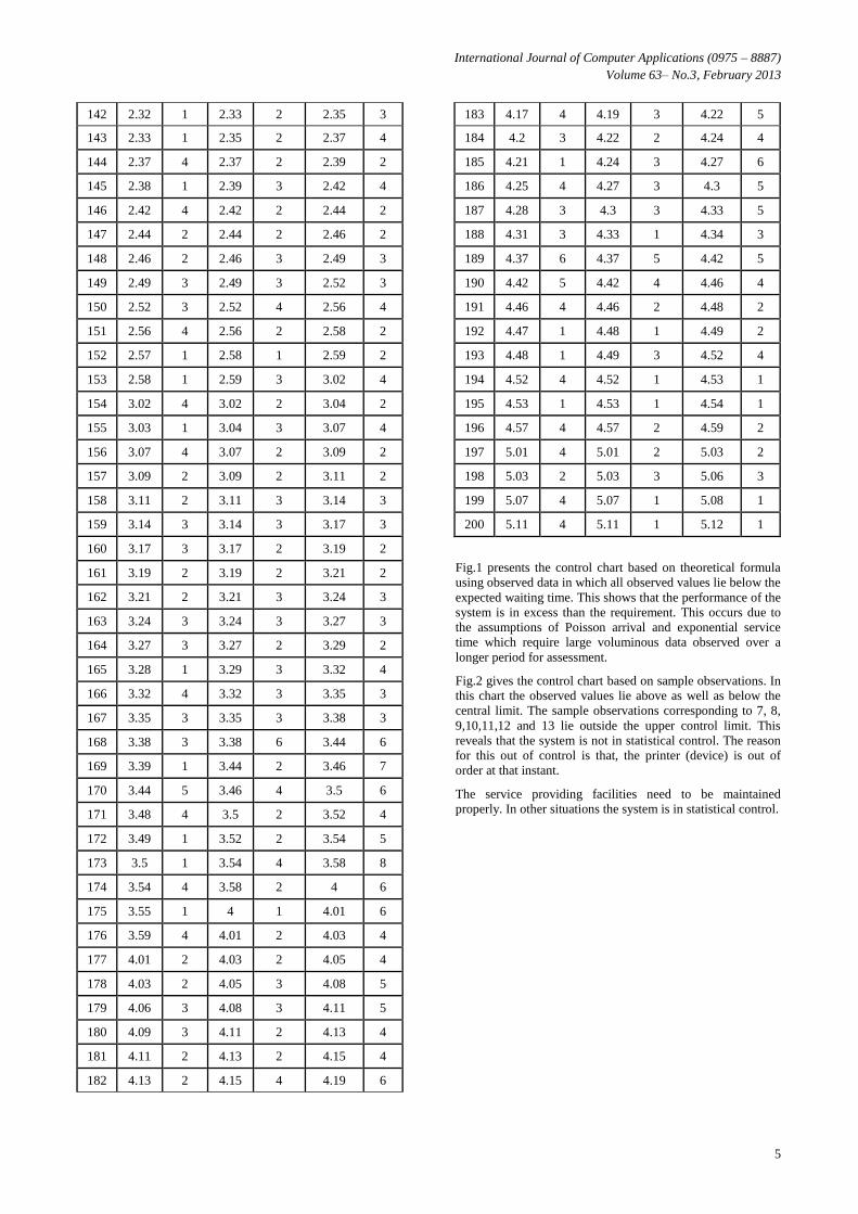
Table.3 Observed waiting time of customers

I II III IV V VI VII

1 8.01 1 8.01 4 8.05 4

2 8.03 2 8.05 3 8.08 5

3 8.04 1 8.08 5 8.13 9

4 8.08 4 8.13 4 8.17 9

5 8.09 1 8.17 2 8.19 10

6 8.1 1 8.19 8 8.27 17

7 8.12 2 8.27 7 8.34 22

8 8.16 4 8.34 10 8.44 28

9 8.19 3 8.44 1 8.45 26

10 8.23 4 8.45 3 8.48 25

11 8.25 2 8.48 1 8.49 24

12 8.27 2 8.49 1 8.5 23

13 8.3 3 8.5 1 8.51 21

14 8.33 3 8.51 1 8.52 19

15 8.37 4 8.52 1 8.53 16

16 8.41 4 8.53 2 8.55 14

17 8.44 3 8.55 2 8.57 13

18 8.47 3 8.57 1 8.58 11

19 8.48 1 8.58 2 9 12

20 8.53 5 9 1 9.01 8

21 8.57 4 9.01 2 9.03 6

22 8.58 1 9.03 2 9.05 7

23 8.59 1 9.05 3 9.08 9

24 9.03 4 9.08 2 9.1 7

25 9.04 1 9.1 3 9.13 9

26 9.08 4 9.13 2 9.15 7

27 9.1 2 9.15 4 9.19 9

28 9.12 2 9.19 2 9.21 9

29 9.15 3 9.21 3 9.24 9

30 9.18 3 9.24 2 9.26 8

31 9.2 2 9.26 2 9.28 8

32 9.22 2 9.28 3 9.31 9

33 9.26 4 9.31 2 9.33 7

34 9.29 3 9.33 2 9.35 6

35 9.3 1 9.35 1 9.36 6

36 9.34 4 9.36 2 9.38 4

37 9.37 3 9.38 3 9.41 4

38 9.4 3 9.41 2 9.43 3

39 9.46 6 9.46 3 9.49 3

40 9.51 5 9.51 3 9.54 3

41 9.55 4 9.55 6 10.01 6

42 9.56 1 10.01 4 10.05 9

43 9.57 1 10.05 2 10.07 10

44 10.01 4 10.07 2 10.09 8

45 10.02 1 10.09 3 10.12 10

46 10.06 4 10.12 2 10.14 8

47 10.08 2 10.14 2 10.16 8

48 10.1 2 10.16 3 10.19 9

49 10.13 3 10.19 2 10.21 8

50 10.16 3 10.21 3 10.24 8

51 10.2 4 10.24 4 10.28 8

52 10.24 4 10.28 3 10.31 7

53 10.25 1 10.31 5 10.36 11

54 10.29 4 10.36 4 10.4 11

55 10.3 1 10.4 2 10.42 12

56 10.34 4 10.42 1 10.43 9

57 10.36 2 10.43 1 10.44 8

58 10.38 2 10.44 1 10.45 7

59 10.41 3 10.45 2 10.47 6



4

60 10.44 3 10.47 3 10.5 6

61 10.46 2 10.5 4 10.54 8

62 10.48 2 10.54 2 10.56 8

63 10.51 3 10.56 3 10.59 8

64 10.54 3 10.59 2 11.01 7

65 10.55 1 11.01 2 11.03 8

66 10.59 4 11.03 3 11.06 7

67 11.02 3 11.06 2 11.08 6

68 11.05 3 11.08 1 11.09 4

69 11.11 6 11.11 1 11.12 1

70 11.16 5 11.16 4 11.2 4

71 11.2 4 11.2 2 11.22 2

72 11.21 1 11.22 5 11.27 6

73 11.22 1 11.27 3 11.3 8

74 11.26 4 11.3 2 11.32 6

75 11.27 1 11.32 3 11.35 8

76 11.31 4 11.35 2 11.37 6

77 11.33 2 11.37 4 11.41 8

78 11.35 2 11.41 2 11.43 8

79 11.38 3 11.43 3 11.46 8

80 11.41 3 11.46 2 11.48 7

81 11.43 2 11.48 2 11.5 7

82 11.45 2 11.5 3 11.53 8

83 11.49 4 11.53 2 11.55 6

84 11.52 3 11.55 2 11.57 5

85 11.53 1 11.57 1 11.58 5

86 11.57 4 11.58 2 12 3

87 12 3 12 3 12.03 3

88 12.03 3 12.03 2 12.05 2

89 12.09 6 12.09 6 12.15 6

90 12.14 5 12.15 5 12.2 6

91 12.18 4 12.2 7 12.27 9

92 12.19 1 12.27 1 12.28 9

93 12.23 4 12.28 2 12.3 7

94 12.27 4 12.3 2 12.32 5

95 12.28 1 12.32 3 12.35 7

96 12.32 4 12.35 2 12.37 5

97 12.34 2 12.37 2 12.39 5

98 12.36 2 12.39 1 12.4 4

99 12.39 3 12.4 2 12.42 3

100 12.42 3 12.42 2 12.44 2

101 12.46 4 12.46 1 12.47 1

102 12.47 1 12.47 2 12.49 2

103 12.48 1 12.49 2 12.51 3

104 12.52 4 12.52 2 12.54 2

105 12.53 1 12.54 6 1 7

106 12.57 4 1 1 1.01 4

107 12.59 2 1.01 2 1.03 4

108 1.01 2 1.03 2 1.05 4

109 1.04 3 1.05 7 1.12 8

110 1.07 3 1.12 1 1.13 6

111 1.09 2 1.13 2 1.15 6

112 1.11 2 1.15 2 1.17 6

113 1.14 3 1.17 1 1.18 4

114 1.17 3 1.18 2 1.2 3

115 1.18 1 1.2 5 1.25 7

116 1.22 4 1.25 1 1.26 4

117 1.25 3 1.26 2 1.28 3

118 1.28 3 1.28 1 1.29 1

119 1.29 1 1.29 4 1.33 4

120 1.34 5 1.34 4 1.38 4

121 1.38 4 1.38 2 1.4 2

122 1.39 1 1.4 2 1.42 3

123 1.4 1 1.42 3 1.45 5

124 1.44 4 1.45 2 1.47 3

125 1.45 1 1.47 3 1.5 5

126 1.49 4 1.5 2 1.52 3

127 1.51 2 1.52 2 1.54 3

128 1.53 2 1.54 4 1.58 5

129 1.56 3 1.58 3 2.01 5

130 1.59 3 2.01 2 2.03 4

131 2.01 2 2.03 2 2.05 4

132 2.03 2 2.05 3 2.08 5

133 2.07 4 2.08 3 2.11 4

134 2.1 3 2.11 2 2.13 3

135 2.11 1 2.13 3 2.16 5

136 2.15 4 2.16 3 2.19 4

137 2.18 3 2.19 3 2.22 4

138 2.21 3 2.22 6 2.28 7

139 2.22 1 2.28 1 2.29 7

140 2.27 5 2.29 1 2.3 3

141 2.31 4 2.31 2 2.33 2



5

142 2.32 1 2.33 2 2.35 3

143 2.33 1 2.35 2 2.37 4

144 2.37 4 2.37 2 2.39 2

145 2.38 1 2.39 3 2.42 4

146 2.42 4 2.42 2 2.44 2

147 2.44 2 2.44 2 2.46 2

148 2.46 2 2.46 3 2.49 3

149 2.49 3 2.49 3 2.52 3

150 2.52 3 2.52 4 2.56 4

151 2.56 4 2.56 2 2.58 2

152 2.57 1 2.58 1 2.59 2

153 2.58 1 2.59 3 3.02 4

154 3.02 4 3.02 2 3.04 2

155 3.03 1 3.04 3 3.07 4

156 3.07 4 3.07 2 3.09 2

157 3.09 2 3.09 2 3.11 2

158 3.11 2 3.11 3 3.14 3

159 3.14 3 3.14 3 3.17 3

160 3.17 3 3.17 2 3.19 2

161 3.19 2 3.19 2 3.21 2

162 3.21 2 3.21 3 3.24 3

163 3.24 3 3.24 3 3.27 3

164 3.27 3 3.27 2 3.29 2

165 3.28 1 3.29 3 3.32 4

166 3.32 4 3.32 3 3.35 3

167 3.35 3 3.35 3 3.38 3

168 3.38 3 3.38 6 3.44 6

169 3.39 1 3.44 2 3.46 7

170 3.44 5 3.46 4 3.5 6

171 3.48 4 3.5 2 3.52 4

172 3.49 1 3.52 2 3.54 5

173 3.5 1 3.54 4 3.58 8

174 3.54 4 3.58 2 4 6

175 3.55 1 4 1 4.01 6

176 3.59 4 4.01 2 4.03 4

177 4.01 2 4.03 2 4.05 4

178 4.03 2 4.05 3 4.08 5

179 4.06 3 4.08 3 4.11 5

180 4.09 3 4.11 2 4.13 4

181 4.11 2 4.13 2 4.15 4

182 4.13 2 4.15 4 4.19 6

183 4.17 4 4.19 3 4.22 5

184 4.2 3 4.22 2 4.24 4

185 4.21 1 4.24 3 4.27 6

186 4.25 4 4.27 3 4.3 5

187 4.28 3 4.3 3 4.33 5

188 4.31 3 4.33 1 4.34 3

189 4.37 6 4.37 5 4.42 5

190 4.42 5 4.42 4 4.46 4

191 4.46 4 4.46 2 4.48 2

192 4.47 1 4.48 1 4.49 2

193 4.48 1 4.49 3 4.52 4

194 4.52 4 4.52 1 4.53 1

195 4.53 1 4.53 1 4.54 1

196 4.57 4 4.57 2 4.59 2

197 5.01 4 5.01 2 5.03 2

198 5.03 2 5.03 3 5.06 3

199 5.07 4 5.07 1 5.08 1

200 5.11 4 5.11 1 5.12 1

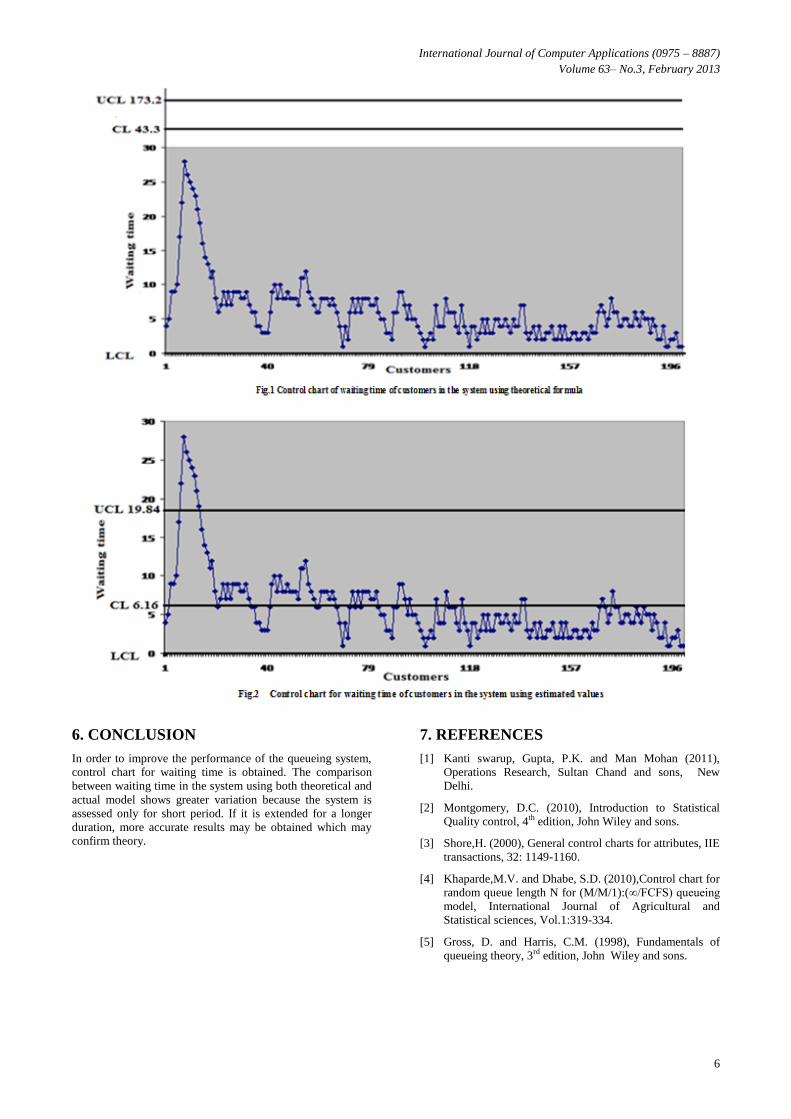
Fig.1 presents the control chart based on theoretical formula

using observed data in which all observed values lie below the

expected waiting time. This shows that the performance of the

system is in excess than the requirement. This occurs due to

the assumptions of Poisson arrival and exponential service

time which require large voluminous data observed over a

longer period for assessment.

Fig.2 gives the control chart based on sample observations. In

this chart the observed values lie above as well as below the

central limit. The sample observations corresponding to 7, 8,

9,10,11,12 and 13 lie outside the upper control limit. This

reveals that the system is not in statistical control. The reason

for this out of control is that, the printer (device) is out of

order at that instant.

The service providing facilities need to be maintained

properly. In other situations the system is in statistical control.



6

6. CONCLUSION

In order to improve the performance of the queueing system,

control chart for waiting time is obtained. The comparison

between waiting time in the system using both theoretical and

actual model shows greater variation because the system is

assessed only for short period. If it is extended for a longer

duration, more accurate results may be obtained which may

confirm theory.

7. REFERENCES

[1] Kanti swarup, Gupta, P.K. and Man Mohan (2011),

Operations Research, Sultan Chand and sons, New

Delhi.

[2] Montgomery, D.C. (2010), Introduction to Statistical

Quality control, 4th edition, John Wiley and sons.

[3] Shore,H. (2000), General control charts for attributes, IIE

transactions, 32: 1149-1160.

[4] Khaparde,M.V. and Dhabe, S.D. (2010),Control chart for

random queue length N for (M/M/1):(∞/FCFS) queueing

model, International Journal of Agricultural and

Statistical sciences, Vol.1:319-334.

[5] Gross, D. and Harris, C.M. (1998), Fundamentals of

queueing theory, 3rd edition, John Wiley and sons.

Documents

Control Chart for Waiting Time in System of (M/M/1