Embed Size (px)
Citation preview
1
CONTROL AND IMPLEMENTATION OF A SINGLE WHEEL HOLONOMIC VEHICLE
RAFAEL PUERTA RAMÍREZ
BOGOTÁ D.C.
PONTIFICIA UNIVERSIDAD JAVERIANA
FACULTY OF ENGINEERING
DEPARTMENT OF ELECTRONICS
NOVEMBER 2013
2
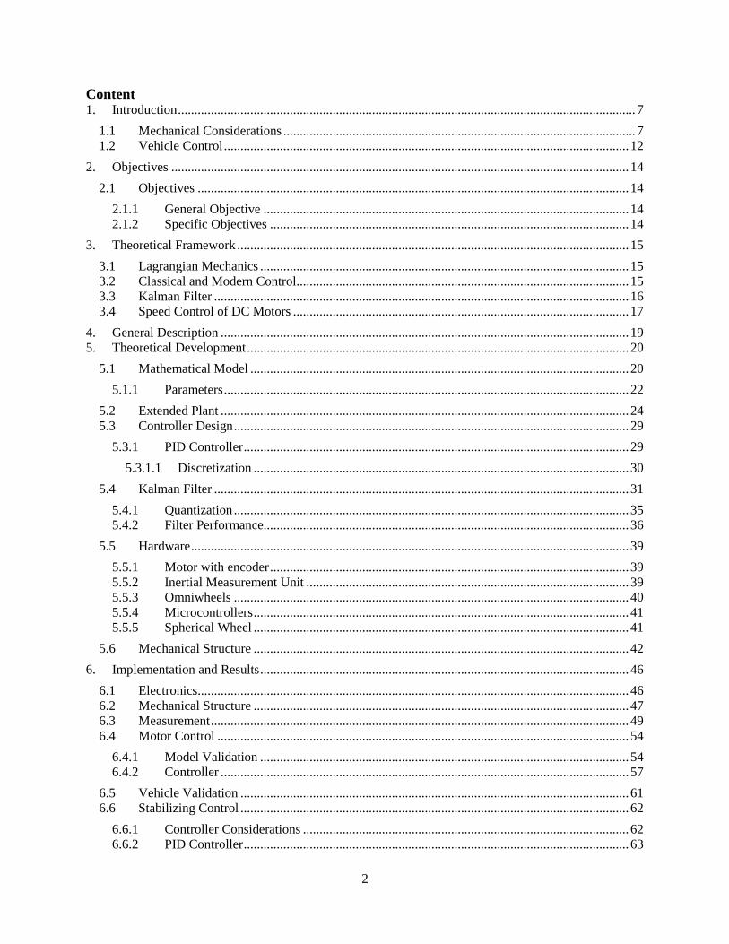
Content 1. Introduction ........................................................................................................................................... 7
1.1 Mechanical Considerations ........................................................................................................... 7
1.2 Vehicle Control ........................................................................................................................... 12
2. Objectives ........................................................................................................................................... 14
2.1 Objectives ................................................................................................................................... 14
2.1.1 General Objective ............................................................................................................... 14
2.1.2 Specific Objectives ............................................................................................................. 14
3. Theoretical Framework ....................................................................................................................... 15
3.1 Lagrangian Mechanics ................................................................................................................ 15
3.2 Classical and Modern Control..................................................................................................... 15
3.3 Kalman Filter .............................................................................................................................. 16
3.4 Speed Control of DC Motors ...................................................................................................... 17
4. General Description ............................................................................................................................ 19
5. Theoretical Development .................................................................................................................... 20
5.1 Mathematical Model ................................................................................................................... 20
5.1.1 Parameters ........................................................................................................................... 22
5.2 Extended Plant ............................................................................................................................ 24
5.3 Controller Design ........................................................................................................................ 29
5.3.1 PID Controller ..................................................................................................................... 29
5.3.1.1 Discretization .................................................................................................................. 30
5.4 Kalman Filter .............................................................................................................................. 31
5.4.1 Quantization ........................................................................................................................ 35
5.4.2 Filter Performance............................................................................................................... 36
5.5 Hardware ..................................................................................................................................... 39
5.5.1 Motor with encoder ............................................................................................................. 39
5.5.2 Inertial Measurement Unit .................................................................................................. 39
5.5.3 Omniwheels ........................................................................................................................ 40
5.5.4 Microcontrollers .................................................................................................................. 41
5.5.5 Spherical Wheel .................................................................................................................. 41
5.6 Mechanical Structure .................................................................................................................. 42
6. Implementation and Results ................................................................................................................ 46
6.1 Electronics ................................................................................................................................... 46
6.2 Mechanical Structure .................................................................................................................. 47
6.3 Measurement ............................................................................................................................... 49
6.4 Motor Control ............................................................................................................................. 54
6.4.1 Model Validation ................................................................................................................ 54
6.4.2 Controller ............................................................................................................................ 57
6.5 Vehicle Validation ...................................................................................................................... 61
6.6 Stabilizing Control ...................................................................................................................... 62
6.6.1 Controller Considerations ................................................................................................... 62
6.6.2 PID Controller ..................................................................................................................... 63
3
6.7 Omnidirectionality ...................................................................................................................... 65
7. Conclusions ......................................................................................................................................... 67
8. References ........................................................................................................................................... 68
9. Annexes............................................................................................................................................... 70
9.1 Annex A – Lagrangian Mechanics .............................................................................................. 70
9.1.1 Generalized Coordinates ..................................................................................................... 70
9.1.2 Hamilton´s Principle ........................................................................................................... 70
9.1.3 Euler-Lagrange equations of motion for conservative systems .......................................... 71
9.1.4 Euler-Lagrange equations of motion for non-conservative systems ................................... 72
9.2 Annex B – Discrete Kalman Filter Gain Derivation ................................................................... 73
9.3 Annex C – Linearization ............................................................................................................. 78
9.4 Annex D - SolidWorks Technical Drawings .............................................................................. 80
9.5 Annex E – Schematic and PCB Layouts ..................................................................................... 89
9.6 Annex F – Mechanical Structure ................................................................................................ 91
9.7 Annex G – Nonlinear Vehicle Simulink Block Diagram ............................................................ 93
4
Table of Figures
Figure 1. Example of a non-holonomic vehicle and a holonomic vehicle. ................................................... 7
Figure 2. a) Universal omnidirectional wheel, b) Universal omnidirectional double wheel , c) 45° swedish
wheel [17]. .................................................................................................................................................... 8
Figure 3. a) Omnidirectional robot with universal omnidirectional wheels b) Omnidirectional Robot
'Uranus' developed in 1985 at the Robotics Institute of the Carnegie-Mellon University. ........................... 9
Figure 4. Locomotion mechanism of the 'Ballbot' Robot [1]. ..................................................................... 10
Figure 5. a) Force transfer mechanism of the ‘B.B. Rider’ robot, b) Lateral view of the mechanism, c)
Diagram of relationship between the mechanism and the spherical wheel. ................................................ 10
Figure 6. Implementation proposed in [7] using omnidirectional wheels................................................... 11
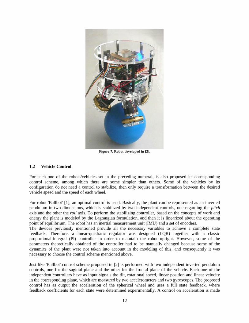
Figure 7. Robot developed in [2]. ............................................................................................................... 12
Figure 8. H-Bridge with a DC motor as load [19]. ..................................................................................... 18
Figure 9. a) The signal S is active. b) During the switching the current stored by the motor is discharged
through the diodes D2 and D3. c) The signal S is inactive. d) During the switching the current stored by
the motor is discharged through the diodes D1 and D4 [19]. ..................................................................... 18
Figure 10. Block diagram. .......................................................................................................................... 19
Figure 11. Simplified model [22]. ............................................................................................................... 20
Figure 12. Complete friction model. ........................................................................................................... 21
Figure 13. System behavior. ....................................................................................................................... 23
Figure 14. System energy. .......................................................................................................................... 24
Figure 15. DC motor model (Simulink). ..................................................................................................... 25
Figure 16. Motor friction model. ................................................................................................................ 27
Figure 17. DC motor complete model (Simulink). ..................................................................................... 27
Figure 18. Motors setup. ............................................................................................................................. 28
Figure 19. Total torque. .............................................................................................................................. 28
Figure 20. Extended plant with a controller. ............................................................................................... 29
Figure 21. System behavior in closed-loop with the selected controller. ................................................... 30
Figure 22. Accelerometer raw measurement. ............................................................................................. 34
Figure 23. Gyroscope raw measurement. .................................................................................................... 34
Figure 24. Gyroscope filtered measurement. .............................................................................................. 35
Figure 25. Extended plant with a Kalman filter, quantization effect, and discrete controller. ................... 37
Figure 26. Simulation comparison 1. .......................................................................................................... 38
Figure 27. Simulation comparison 2. .......................................................................................................... 38
Figure 28. Selected motor. .......................................................................................................................... 39
Figure 29. Inertial Measurement Unit. ........................................................................................................ 40
Figure 30. VEX® Omni Wheel. ................................................................................................................. 40
Figure 31. VEX® drive shafts (left) and shaft collars (right). .................................................................... 41
Figure 32. Hex hub. .................................................................................................................................... 41
Figure 33. Spherical wheels. Kickball (left) and basketball (right). ........................................................... 42
Figure 34. Sketch for dimensioning the structure. ...................................................................................... 43
Figure 35. Pair of pieces to hold the motors. .............................................................................................. 44
Figure 36. Structure bottom level (horizontal plane). ................................................................................. 44
Figure 37. Assembly of structure bottom level with all the pieces and a motor. ........................................ 45
Figure 38. Overall diagram of electronics. ................................................................................................. 46
Figure 39. Circuit board. ............................................................................................................................. 47
Figure 40. Structure. ................................................................................................................................... 48
Figure 41. Experimental setup to test the Kalman filter. ............................................................................ 51
Figure 42. Linear potentiometer.................................................................................................................. 52
Figure 43. Example of stationary position test results. ............................................................................... 52
Figure 44. Example of medium velocity test results. .................................................................................. 53
5
Figure 45. Example of fast velocity test results. ......................................................................................... 53
Figure 46. Transient response of the model and motor with step inputs of 3V, 6V and 9V. ...................... 55
Figure 47. Transient response of the model and motor with ramp inputs with slopes of 1.63V/sec and
2.45V/sec. ................................................................................................................................................... 56
Figure 48. Algorithm flowchart. ................................................................................................................. 59
Figure 49. Motor step response comparison. .............................................................................................. 60
Figure 50. Motor ramp response comparison. ............................................................................................ 61
Figure 51. Comparison between real vehicle and simulations over the range [0, π/12] rads...................... 62
Figure 52. Comparison of vehicle tilt in actual implementation. ................................................................ 64
Figure 53. Comparison of virtual wheel speed in actual implementation. .................................................. 64
Figure 54. Comparison of controller output in actual implementation. ...................................................... 65
Figure 55. Omnidirectionality test. ............................................................................................................. 66
Figure 56. Research suggestion [35]. .......................................................................................................... 67
6
Table of Tables
Table 1. Model parameters. ........................................................................................................................ 20
Table 2. Motor parameters. ......................................................................................................................... 25
Table 3. Missing motor parameters............................................................................................................. 26
Table 4. Average values of standard deviations of process and measurement noise. ................................. 33
Table 5. Average accelerometer measurements. ......................................................................................... 36
Table 6. Simulations results. ....................................................................................................................... 37
Table 7. Motor specifications...................................................................................................................... 39
Table 8. IMU specifications. ....................................................................................................................... 40
Table 9. Principal dimensions of the vehicle. ............................................................................................. 49
Table 10. Accelerometer static operating ranges. ....................................................................................... 50
Table 11. Average values of mean squared errors and ratio between these. ............................................... 54
Table 12. Modified parameters of the motor model. .................................................................................. 55
Table 13. Average Percent values. .............................................................................................................. 56
Table 14. Average values of mean squared errors and percent error between these. ................................. 61
7
1. Introduction
In mobile robotics is of vital importance the ease with which a robot can move from one place to another.
There are several types of locomotion mechanisms on a solid surface that provide different possibilities.
Among the most common ones there are wheels, legs and tracks (e.g. continuous tracks or caterpillar
tracks).
In robotics, the holonomic refers to the relationship between the number of total degrees of freedom and
the number of controllable degrees of freedom (number of actuators). If the quantity of controllable
degrees of freedom is equal to the total, it is said that a robot is holonomic, otherwise it is said that the
robot is non-holonomic. Etymologically, the interpretation of the holonomy term is quite ambiguous,
however, what it’s wanted to note is that a holonomic vehicle that moves on a flat surface is the one
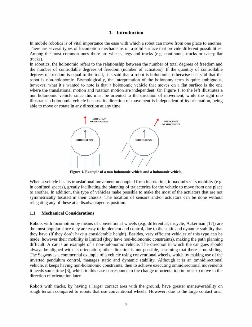
where the translational motion and rotation motion are independent. On Figure 1, to the left illustrates a
non-holonomic vehicle since this must be oriented to the direction of movement, while the right one
illustrates a holonomic vehicle because its direction of movement is independent of its orientation, being
able to move or rotate in any direction at any time.
Figure 1. Example of a non-holonomic vehicle and a holonomic vehicle.
When a vehicle has its translational movement uncoupled from its rotation, it maximizes its mobility (e.g.
in confined spaces), greatly facilitating the planning of trajectories for the vehicle to move from one place
to another. In addition, this type of vehicles make possible to make the most of the actuators that are not
symmetrically located in their chassis. The location of sensors and/or actuators can be done without
relegating any of these at a disadvantageous position.
1.1 Mechanical Considerations
Robots with locomotion by means of conventional wheels (e.g. differential, tricycle, Ackerman [17]) are
the most popular since they are easy to implement and control, due to the static and dynamic stability that
they have (if they don’t have a considerable height). Besides, very efficient vehicles of this type can be
made, however their mobility is limited (they have non-holonomic constraints), making the path planning
difficult. A car is an example of a non-holonomic vehicle. The direction in which the car goes should
always be aligned with its orientation; other direction is not possible, assuming that there is no sliding.
The Segway is a commercial example of a vehicle using conventional wheels, which by making use of the
inverted pendulum control, manages static and dynamic stability. Although it is an omnidirectional
vehicle, it keeps having non-holonomic constraints, then to achieve executing omnidirectional movements
it needs some time [3], which in this case corresponds to the change of orientation in order to move in the
direction of orientation later.
Robots with tracks, by having a larger contact area with the ground, have greater maneuverability on
rough terrain compared to robots that use conventional wheels. However, due to the large contact area,
8
when an orientation change is performed the tracks slip extensively against the ground. Consequently, the
exact center of rotation is difficult to predict and the change of position and orientation are subject to
variations in the friction of the ground. Furthermore, straight-line movement control is difficult to
achieve, and then the usage of this type of robots for estimative navigation would provide inaccurate
results. Regarding to energy consumption, this type of locomotion is inefficient in uniform terrain,
however in rough terrains is reasonably efficient.
Robots with legs have several characteristics that make them superior in some aspects to robots with other
configurations for its mobility. Among the most notable are the omnidirectionality that they have to move
and the ability to overcome obstacles (e.g. climb stairs). Nevertheless, they are very difficult to control
and implement since they have many degrees of freedom, which usually makes them slow and only
keeping the static stability, is demanding. Another disadvantage they have is their high-energy
consumption.
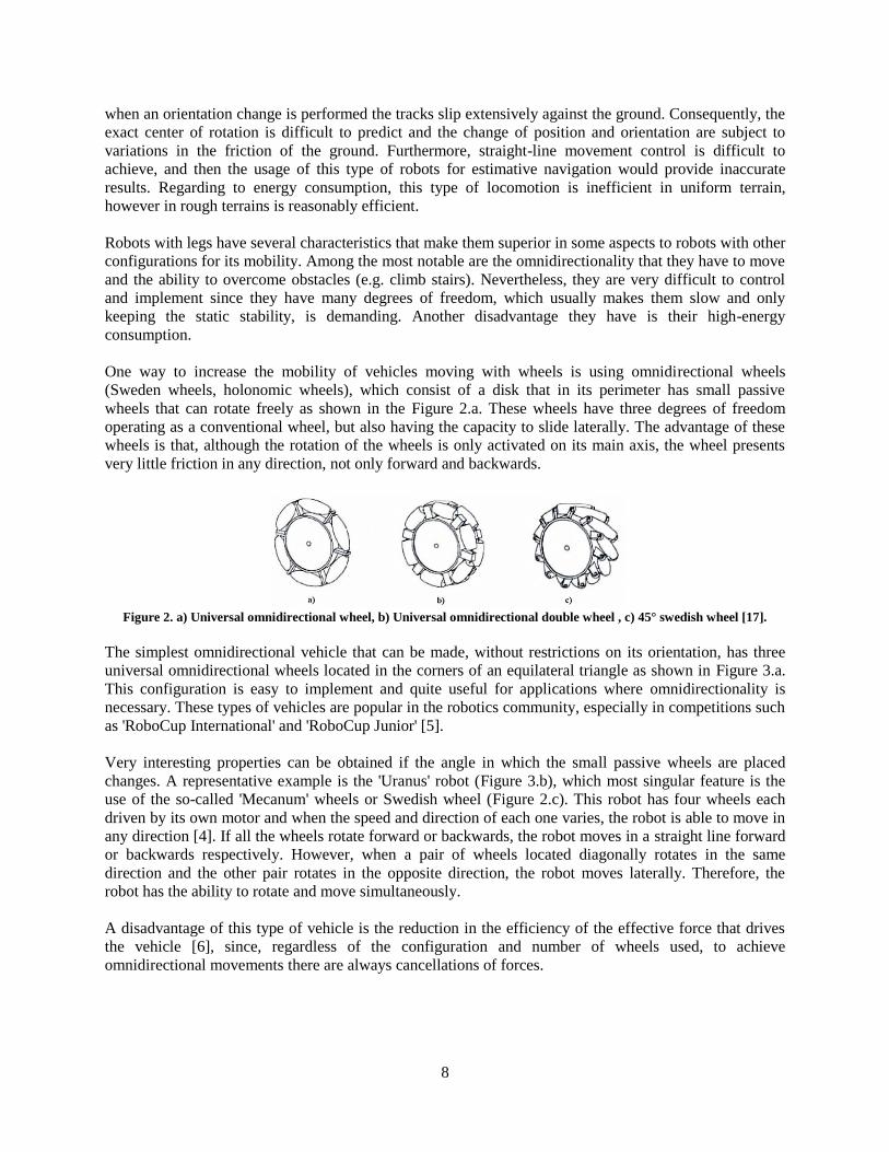
One way to increase the mobility of vehicles moving with wheels is using omnidirectional wheels
(Sweden wheels, holonomic wheels), which consist of a disk that in its perimeter has small passive
wheels that can rotate freely as shown in the Figure 2.a. These wheels have three degrees of freedom
operating as a conventional wheel, but also having the capacity to slide laterally. The advantage of these
wheels is that, although the rotation of the wheels is only activated on its main axis, the wheel presents
very little friction in any direction, not only forward and backwards.
Figure 2. a) Universal omnidirectional wheel, b) Universal omnidirectional double wheel , c) 45° swedish wheel [17].
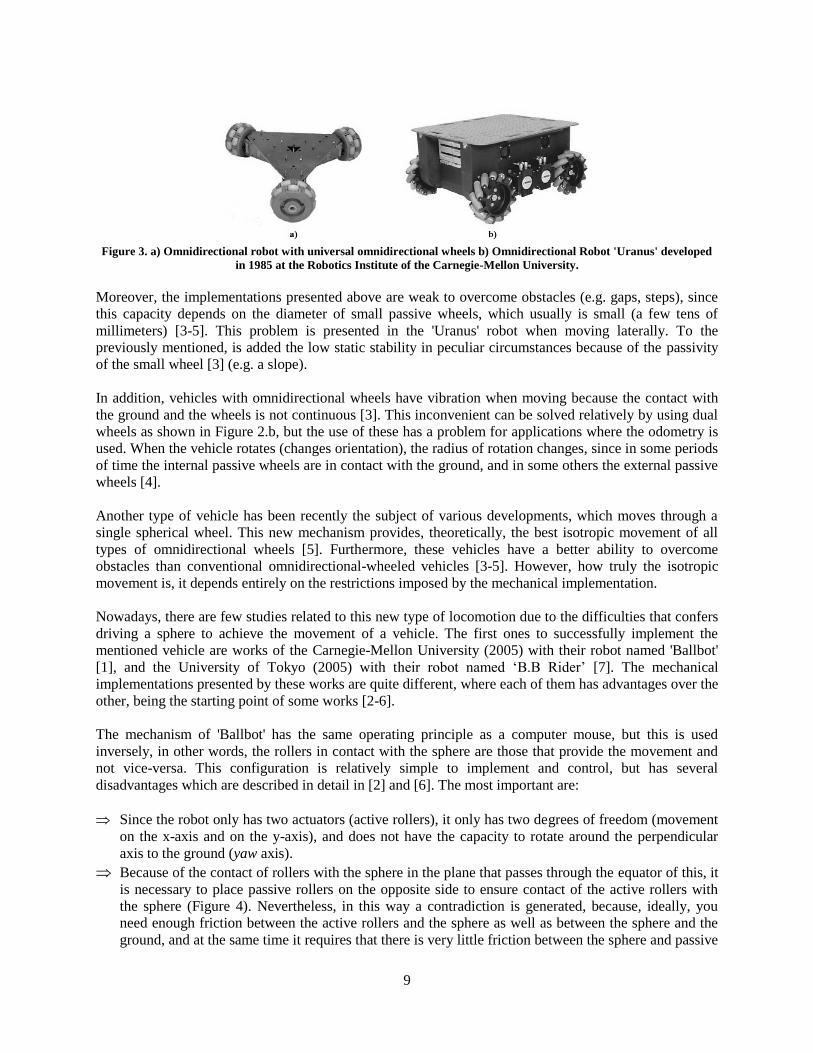
The simplest omnidirectional vehicle that can be made, without restrictions on its orientation, has three
universal omnidirectional wheels located in the corners of an equilateral triangle as shown in Figure 3.a.
This configuration is easy to implement and quite useful for applications where omnidirectionality is
necessary. These types of vehicles are popular in the robotics community, especially in competitions such
as 'RoboCup International' and 'RoboCup Junior' [5].
Very interesting properties can be obtained if the angle in which the small passive wheels are placed
changes. A representative example is the 'Uranus' robot (Figure 3.b), which most singular feature is the
use of the so-called 'Mecanum' wheels or Swedish wheel (Figure 2.c). This robot has four wheels each
driven by its own motor and when the speed and direction of each one varies, the robot is able to move in
any direction [4]. If all the wheels rotate forward or backwards, the robot moves in a straight line forward
or backwards respectively. However, when a pair of wheels located diagonally rotates in the same
direction and the other pair rotates in the opposite direction, the robot moves laterally. Therefore, the
robot has the ability to rotate and move simultaneously.
A disadvantage of this type of vehicle is the reduction in the efficiency of the effective force that drives
the vehicle [6], since, regardless of the configuration and number of wheels used, to achieve
omnidirectional movements there are always cancellations of forces.
9
Figure 3. a) Omnidirectional robot with universal omnidirectional wheels b) Omnidirectional Robot 'Uranus' developed
in 1985 at the Robotics Institute of the Carnegie-Mellon University.
Moreover, the implementations presented above are weak to overcome obstacles (e.g. gaps, steps), since
this capacity depends on the diameter of small passive wheels, which usually is small (a few tens of
millimeters) [3-5]. This problem is presented in the 'Uranus' robot when moving laterally. To the
previously mentioned, is added the low static stability in peculiar circumstances because of the passivity
of the small wheel [3] (e.g. a slope).
In addition, vehicles with omnidirectional wheels have vibration when moving because the contact with
the ground and the wheels is not continuous [3]. This inconvenient can be solved relatively by using dual
wheels as shown in Figure 2.b, but the use of these has a problem for applications where the odometry is
used. When the vehicle rotates (changes orientation), the radius of rotation changes, since in some periods
of time the internal passive wheels are in contact with the ground, and in some others the external passive
wheels [4].
Another type of vehicle has been recently the subject of various developments, which moves through a
single spherical wheel. This new mechanism provides, theoretically, the best isotropic movement of all
types of omnidirectional wheels [5]. Furthermore, these vehicles have a better ability to overcome
obstacles than conventional omnidirectional-wheeled vehicles [3-5]. However, how truly the isotropic
movement is, it depends entirely on the restrictions imposed by the mechanical implementation.
Nowadays, there are few studies related to this new type of locomotion due to the difficulties that confers
driving a sphere to achieve the movement of a vehicle. The first ones to successfully implement the
mentioned vehicle are works of the Carnegie-Mellon University (2005) with their robot named 'Ballbot'
[1], and the University of Tokyo (2005) with their robot named ‘B.B Rider’ [7]. The mechanical
implementations presented by these works are quite different, where each of them has advantages over the
other, being the starting point of some works [2-6].
The mechanism of 'Ballbot' has the same operating principle as a computer mouse, but this is used
inversely, in other words, the rollers in contact with the sphere are those that provide the movement and
not vice-versa. This configuration is relatively simple to implement and control, but has several
disadvantages which are described in detail in [2] and [6]. The most important are:
Since the robot only has two actuators (active rollers), it only has two degrees of freedom (movement
on the x-axis and on the y-axis), and does not have the capacity to rotate around the perpendicular
axis to the ground (yaw axis).
Because of the contact of rollers with the sphere in the plane that passes through the equator of this, it
is necessary to place passive rollers on the opposite side to ensure contact of the active rollers with
the sphere (Figure 4). Nevertheless, in this way a contradiction is generated, because, ideally, you
need enough friction between the active rollers and the sphere as well as between the sphere and the
ground, and at the same time it requires that there is very little friction between the sphere and passive
10
rollers. Since you cannot simultaneously satisfy these two demands, the ball wears out quickly due to
the contact with the passive rollers mainly.
Figure 4. Locomotion mechanism of the 'Ballbot' Robot [1].
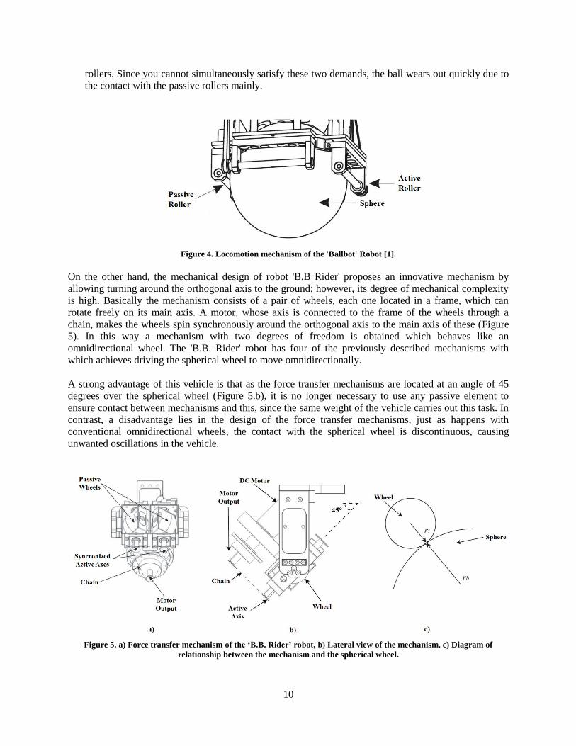
On the other hand, the mechanical design of robot 'B.B Rider' proposes an innovative mechanism by
allowing turning around the orthogonal axis to the ground; however, its degree of mechanical complexity
is high. Basically the mechanism consists of a pair of wheels, each one located in a frame, which can
rotate freely on its main axis. A motor, whose axis is connected to the frame of the wheels through a
chain, makes the wheels spin synchronously around the orthogonal axis to the main axis of these (Figure
5). In this way a mechanism with two degrees of freedom is obtained which behaves like an
omnidirectional wheel. The 'B.B. Rider' robot has four of the previously described mechanisms with
which achieves driving the spherical wheel to move omnidirectionally.
A strong advantage of this vehicle is that as the force transfer mechanisms are located at an angle of 45
degrees over the spherical wheel (Figure 5.b), it is no longer necessary to use any passive element to
ensure contact between mechanisms and this, since the same weight of the vehicle carries out this task. In
contrast, a disadvantage lies in the design of the force transfer mechanisms, just as happens with
conventional omnidirectional wheels, the contact with the spherical wheel is discontinuous, causing
unwanted oscillations in the vehicle.
Figure 5. a) Force transfer mechanism of the ‘B.B. Rider’ robot, b) Lateral view of the mechanism, c) Diagram of
relationship between the mechanism and the spherical wheel.

11
The vehicles proposed in [3] and [5] use an arrangement of three spheres forming an equilateral triangle,
greatly increasing the stability of these. However, these share the problems with the vehicle presented in
[1] so, even though the contact area between the actuator and the sphere is lower, the spherical wheels,
just like the actuators, they wear out. Besides, these vehicles still need passive elements to ensure contact
between the parts mentioned above.
Moreover, to ensure that the vehicle moves without error, each arrangement consisting of the sphere and
its corresponding actuator must be identical, which is difficult to achieve.
The mechanical designs presented in [2] and [6] share a very similar approach to the one presented in [7],
but these are much simpler because it replaces the force transfer mechanisms by omnidirectional wheels,
which provide the same degrees of freedom and greatly facilitate the mechanical implementation.
However, as proposed in [6], just like what happens with 'Ballbot', although it no longer needs passive
elements to function properly, it only uses two actuators limiting the mobility of the vehicle since its
configuration does not allow the change of orientation.
Finally, the mechanical design proposed in [2] is superior to all the mentioned above as it makes use of
three actuators which assures its holonomicity, enjoying the advantages described of the ‘B.B Rider’
vehicle, but with an easier implementation for the use of omnidirectional wheels as mentioned previously.
The three actuators are placed so that the three wheels are fixed symmetrically at intervals of 120°. Each
wheel is located at certain angle φ, being perpendicular to the tangent plane to the spherical wheel as
shown in Figure 6. With this configuration, the robot has three degrees of freedom being possible to
decouple the translational motion and the rotational motion.
Figure 6. Implementation proposed in [7] using omnidirectional wheels.
Due to the earlier observations, to develop the proposed vehicle primarily will be considered the proposed
in [2]. Figure 7 shows the robot developed in [2].
12
Figure 7. Robot developed in [2].
1.2 Vehicle Control
For each one of the robots/vehicles set in the preceding numeral, is also proposed its corresponding
control scheme, among which there are some simpler than others. Some of the vehicles by its
configuration do not need a control to stabilize, then only require a transformation between the desired
vehicle speed and the speed of each wheel.
For robot 'Ballbot' [1], an optimal control is used. Basically, the plant can be represented as an inverted
pendulum in two dimensions, which is stabilized by two independent controls, one regarding the pitch
axis and the other the roll axis. To perform the stabilizing controller, based on the concepts of work and
energy the plant is modeled by the Lagrangian formulation, and then it is linearized about the operating
point of equilibrium. The robot has an inertial measurement unit (IMU) and a set of encoders.
The devices previously mentioned provide all the necessary variables to achieve a complete state
feedback. Therefore, a linear-quadratic regulator was designed (LQR) together with a classic
proportional-integral (PI) controller in order to maintain the robot upright. However, some of the
parameters theoretically obtained of the controller had to be manually changed because some of the
dynamics of the plant were not taken into account in the modeling of this, and consequently it was
necessary to choose the control scheme mentioned above.
Just like 'Ballbot' control scheme proposed in [2] is performed with two independent inverted pendulum
controls, one for the sagittal plane and the other for the frontal plane of the vehicle. Each one of the
independent controllers have as input signals the tilt, rotational speed, linear position and linear velocity
in the corresponding plane, which are measured by two accelerometers and two gyroscopes. The proposed
control has as output the acceleration of the spherical wheel and uses a full state feedback, where
feedback coefficients for each state were determined experimentally. A control on acceleration is made
13
and not on the torque since according to the authors the resulting control presents more robustness.
Afterwards, by numerical integration, the desired speed commands are obtained, and through a linear
transformation the corresponding speed of each omnidirectional wheel is assigned.
In the works [3-5] only linear transformations are performed on the desired speed to obtain the speed
commands for each actuator since stabilizing controls are no longer needed because their mechanical
configurations discussed above, do not require these.
The control approach presented in [4] uses the speed in the x-axis, the speed in y-axis and the angular
velocity of rotation ω as inputs. The vehicle has 4 wheels, so through a linear transformation using a
Jacobian matrix, the speed for each wheel is obtained. The control made is simple, however its
implementation is weak since it does not use any kind of feedback to measure the actual speeds.
What was done in [5] is very similar to what was proposed in [4], but only three actuators are used, then
the transformations change, but the concept is the same. On the other hand, here a feedback of the actual
speed of each wheel is made using encoders, achieving a much higher correspondence between the
desired values and actual values of the velocities.
The idea presented in [7] is a little more complicated than the previous ones. Because of its application
(the vehicle is designed to carry a person), as input to the control system a gyroscope is used to measure
the orientation of the vehicle, and the signals coming from a six-axis force-torque sensor are used to
measure the user's center of mass when it moves. The stabilizing control of the plant is not explained in
detail, it is only explained how the desired speed is transmitted to the wheel of the vehicle. Some complex
transformations are made by pseudoinverse matrices between the desired speed of the spherical wheel and
the speed of each force transfer mechanism mentioned above, as done with the desired torques. Although
the approach presented is not simple, the important matter that can be noted is that the relationship of
velocities can be modeled as a transmission relationship given by the ratio relationship of the radiuses of
the spherical wheel and the equivalent wheel that represents the force transfer mechanism (Figure 5.c).
In [8], although all the obtained results were limited to simulations, they present an innovating approach
using a sliding mode control (SMC) for ‘Ballbot’. As well as in [1], to model the plant the use of
Lagrangian mechanics is made, however, the model is not as complete as in [1] since it does not take into
account non-conservative forces that are inherent in the system. One advantage of the proposed control is
its robustness, being as simple as switching between two states (ON-OFF), achieving a great insensitivity
to the variation of the system parameters (uncertainties). Moreover, since the control is not a continuous
function, it manages to take the system to the desired state in finite time, being better than a system with
an asymptotic behavior. However, it’s necessary to be careful with this type of control since it can result
in considerable energy loss and even in the plant damage (actuators).
14
2. Objectives
2.1 Objectives
2.1.1 General Objective Design, implement and validate the control scheme and mechanical structure of a single wheel holonomic
vehicle.
2.1.2 Specific Objectives - Obtain and simulate the electromechanical model of the plant (e.g. MATLAB®, Simulink®).
- Define the mechanical structure of the vehicle and simulate it through software (e.g. Simulink®
SimMechanics, SolidWorks).
- Design a stabilizing controller for the vehicle.
- Build the proposed vehicle and implement the designed controller on an embedded system.
- Define an experimental protocol that allows validating the obtained model of the plant and the
control technique proposed.
15
3. Theoretical Framework
3.1 Lagrangian Mechanics
The Lagrangian mechanics is, basically, just another way of looking at Newtonian mechanics.
The fundamental forces are conservative, and many forces we deal with in daily life are conservative also
(friction being one evident exception). A conservative force can be thought of as a force that conserves
mechanical energy and can be represented as the gradient of a potential. When an object is being affected
only by conservative forces, we can rewrite the Newton’s second law as
or, in vector form, using as the object position vector
The "Lagrangian formulation" of Newtonian mechanics is based on the previous equation, which, again,
is just an alternate form of Newton's laws which is applicable in cases where the forces are conservative.
This simple change is useful because, in general, Newtonian mechanics has a problem: it works very
nicely in cartesian coordinates, but it's difficult to switch to a different coordinate system. The Lagrangian
formulation, in contrast, is independent of the coordinates, and the equations of motion for a non-cartesian
coordinate system can typically be found immediately using it [20].
Mathematical models for physical systems may be derived from energy considerations without applying
Newton´s laws to them. As starting point, in the Lagrangian approach a quantity is defined
called Lagrangian, where K is the kinetic energy and U is the potential energy of the system. The
Lagrangian L in general is function of the time t, and of where is a generalized
coordinate.
To derive Lagrange equations of motion it is necessary to define the generalized coordinates, and to state
Hamilton’s principle (Annex A – Lagrangian Mechanics).
3.2 Classical and Modern Control
Classical and modern control theory is widely used from basic stable systems that need to follow a simple
reference, to complex industrial automation processes because of its relative simple implementation and
easiness of the tuning procedure. Furthermore, thanks to the development of microcontrollers in the last
decades, digital control became very popular because of the straightforwardness in achieving an
acceptable controller and its subsequent implementation.
Modern control theory differs from conventional control theory in that the former can be applied to linear
or nonlinear systems with multiple inputs and multiple outputs, while the latter only is applied to time
invariant linear systems with one input and one output. Also, the modern control theory is essentially an
approach in time domain, while conventional control theory is a complex approach in frequency domain.
However, in many cases the main idea is to use tools provided by modern control theory to simplify
complex systems and approximate them to simpler systems to use classical control theory techniques.
16
First of all, to design a good controller is critical to obtain a model that represents accurately the system to
be controlled. The theory developed to control processes, from the point of view of classical and modern
control, has its essential basis in the knowledge of the dynamics of the process to be controlled. Normally,
these dynamics are expressed using ordinary differential equations, and in the case of linear systems,
Laplace transform is used to obtain a mathematical representation relating the signal to be controlled and
the input signal of the system. This relation is known as transfer function. If the differential equations are
nonlinear and have a known solution, it may be possible to linearize the nonlinear differential equations at
that solution.
The mathematical models may adopt many different forms. Depending on which the system is, a
mathematical model can be more convenient than others. For example, if an optimal approach is taken to
design a controller is better to use a space state representation. On the other hand, for transient response or
frequency response analysis of time invariant linear systems with one input and one output, a transfer
function representation is more suitable.
The accuracy of a model to represent a system is proportional to its complexity. In some cases, a bunch of
equations are used to describe a single system. However, when obtaining a mathematical model it must be
set a trade-off between simplicity and precision. If extreme precision is not required, is preferred to obtain
only one reasonably simplified model. To get a simplified model, it is often necessary to neglect some
physical properties inherent to the system, and if the effects of these neglected properties on the response
are small, it is expected a good match between the mathematical model and the real system.
In general, a good approach is to, first develop a simplified model to obtain a general idea of de solution,
and then get a more complete model and test, with it, the solution obtained previously.
3.3 Kalman Filter
Initially intended for spacecraft navigation, the Kalman filter proved to be quite useful for many other
applications. One of its main applications is to estimate the states of a system that can only be obtained
indirectly or inaccurately by measurement devices. Basically the Kalman filter applies a statistical model
of how the states of a system evolves over time and a statistical model of how the measurements
(observations) that are made are related to these states. The gains used in a Kalman filter are selected to
achieve that, with certain assumptions about the process model used and the measurements, the obtained
estimated states minimizes mean squared error [23]
[ ] ∫
[( )( ) ] ∫ ( )( )
where is the true state, is the estimated state, refers to the observations (noisy measurements)
and is a probability density function. The result of the filter, that is the estimated state , is modeled
as the conditional probability density function which describes the probabilities associated
with given the observation [23]. Differentiating the last expression with respect to and setting
equal to zero gives
∫
17
which, by definition, is the conditional expectation { }. The Kalman filter, and in fact any
mean squared error estimator, computes an estimate which is the conditional expectation, rather than a
most likely value [23].
The Kalman filter essentially is a set of equations that implement a predictor-corrector type estimator that
is optimal in the sense that it minimizes the estimated error covariance, when some presumed conditions
are met. Since it was introduced, the Kalman filter has been the subject of many researches and
applications, mostly in the area of autonomous and assisted navigation. This is thanks, mainly, to
advances in digital computing that made the use of the filter practical [24].
To better understand the way Kalman filter works, and taking into account that the implementation of the
filter will be on an embedded system, all deductions are going to be done in discrete time (Annex B –
Discrete Kalman Filter Gain Derivation).
The reason why Kalman filter is appropriate for balancing robots is that accelerometers are often the
principal measurement devices involved and they are extremely noisy. Using multiple accelerometers and
then combining them with angular velocity measurements from gyroscopes can smooth out the reading
significantly. Further, as mention before, the linear recursive nature of the algorithm guarantees that its
application is simple and efficient.
3.4 Speed Control of DC Motors
Currently, the DC motors are used in wide range of applications due to its easy control and good
performance. Depending on the requirements of the application, the power converter for a DC motor can
be chosen from a series of topologies. A very easy to implement and effective converter is one modulated
with pulse width (PWM). For applications where only motor direction is needed, a single quadrant
converter can be used, but in applications where both directions are needed, a four quadrant converter
must be used [18].
On the other hand, switching converters produces ripple on the current, which is strongly associated with
the switching frequency and the inductance value of the circuit. A large ripple on the current can generate
problems with the switching and even shorten the lifetime of a motor. For these reasons is recommended
that the amplitude of the current´s ripple is kept below the value corresponding to ten percent of the
nominal current of the motor. In general, the amplitude of current´s ripple is reduced when the value of
the circuit inductance is increased or when the switching frequency is increased [19]. Thus, as the motor
cannot be modified, the selection of the switching frequency must be accurate to prevent system failure.
The basic idea behind the switching converters is the control through pulses, where the duration of the
positive and negative pulses is controlled to obtain a desired average output. The four quadrant converters
are widely used for motor control since they allow a flow of current in both directions, and thanks to the
great development in the power switching devices, switching frequencies of 10-20 kHz can be achieved
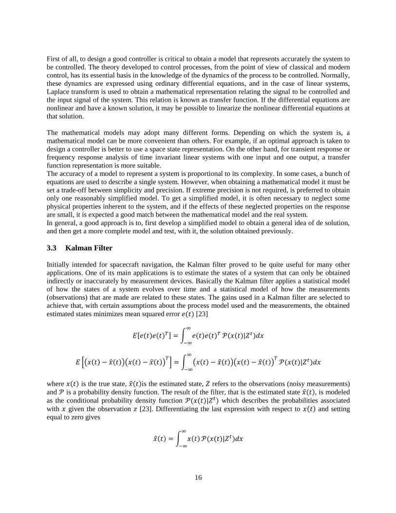
easily, thus the losses are much lower [18]. The topology that is often used is presented in Figure 8, where
the load of a DC motor is represented by the elements L, R and E. The element E is the voltage induced
by the rotor winding which is proportional to the angular velocity, and the elements R and L are the
resistance and inductance of the rotor windings respectively.
18
Figure 8. H-Bridge with a DC motor as load [19].
In the previous topology, the switches (transistors) S1 and S4 are controlled by the same signal , while
the switches S2 and S3 are controlled by the complement of the signal , that is . Thus, when the signal
is active, the motor is polarized in one direction, and when the signal is inactive, the motor is polarized
in the opposite direction. A DC motor is primarily an inductive load, so the switches should be capable of
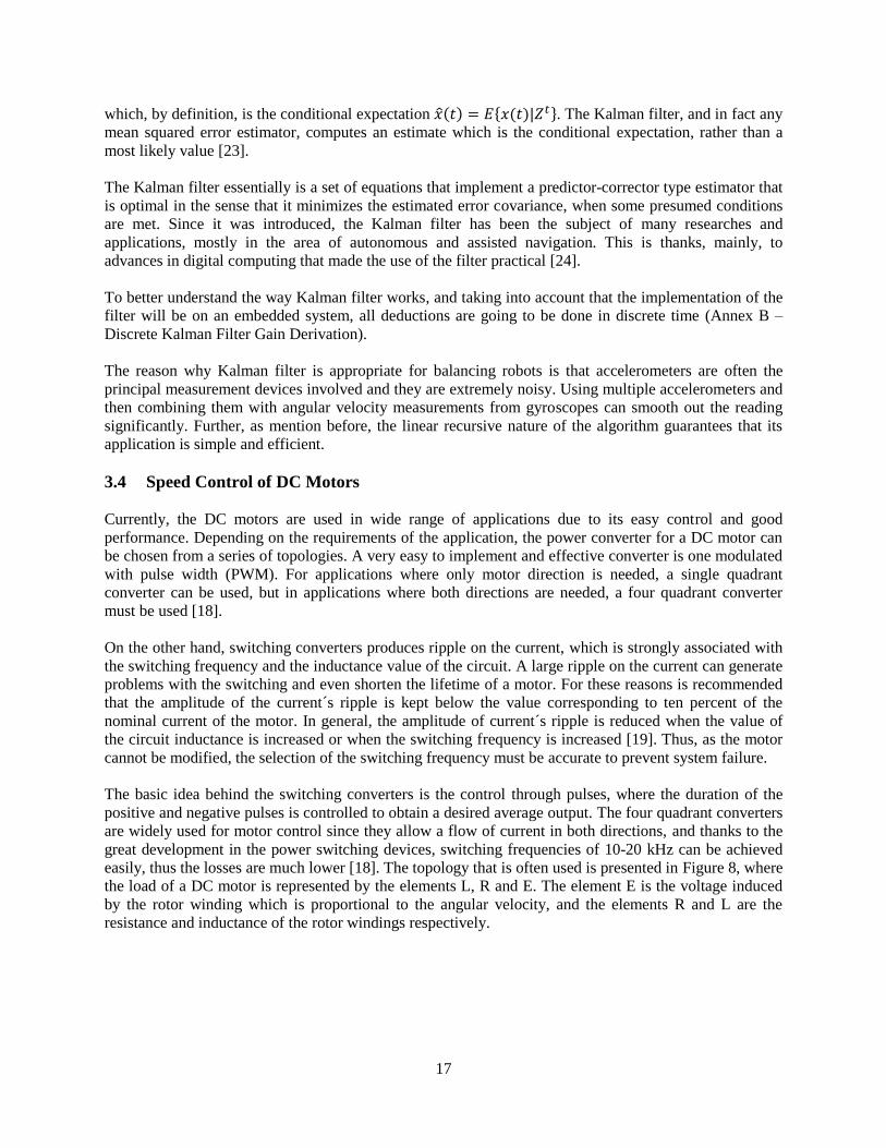
conducting current in both directions, which is achieved through the protection diodes. Figure 9 illustrates
the directions of current during the switching (it should be remembered that under this topology, the
power supply must be able to allow incoming currents).
Figure 9. a) The signal S is active. b) During the switching the current stored by the motor is discharged through the
diodes D2 and D3. c) The signal S is inactive. d) During the switching the current stored by the motor is discharged
through the diodes D1 and D4 [19].
19
4. General Description
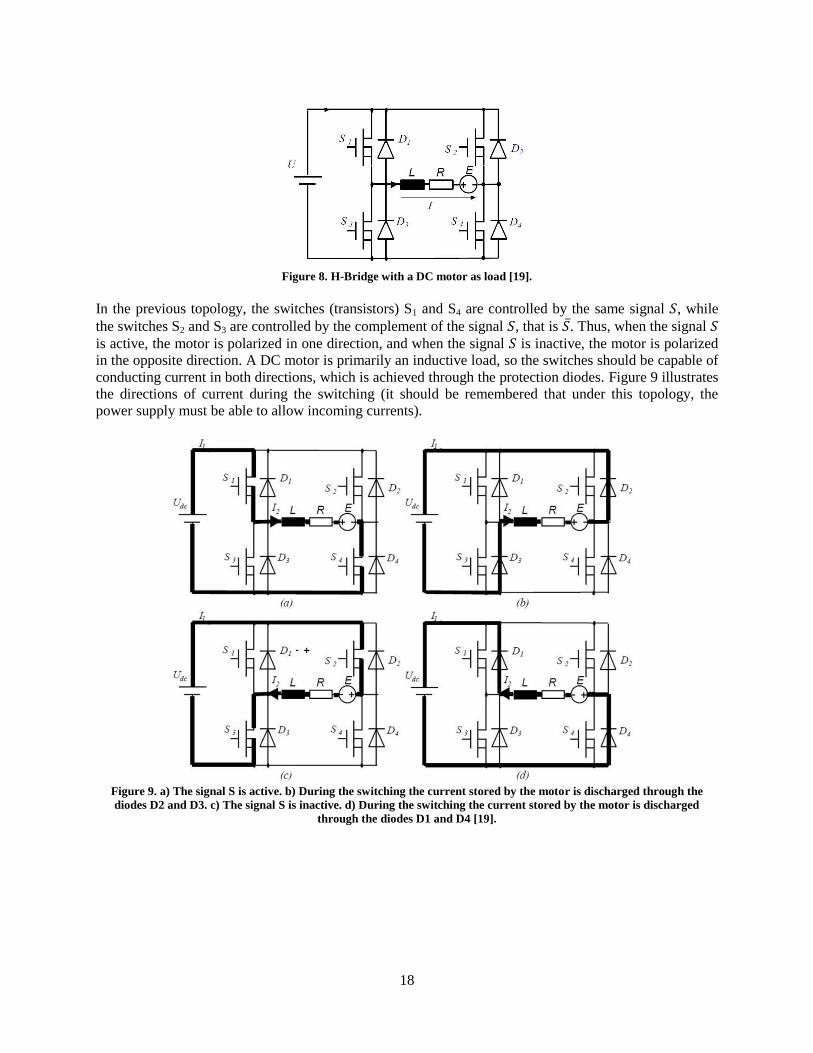
The project itself is, in summary, the construction of the vehicle proposed and the development and
implementation of a control system to stabilize the unstable vehicle. The overall block diagram is shown
in Figure 10.
Figure 10. Block diagram.
Plant: Is the vehicle to be done.
Sensors: These are the devices that give the measurement of the physical variables. Among them are
accelerometers and gyroscopes.
Controller: Is the system that, feeding back the physical variables, generates the control commands in
order to keep the vehicle stable. This control is performed by microcontrollers (digital control).
Actuators: These are the devices that apply the required torque to the ball so the plant holds upright.
Drivers: These are the devices that convert/amplify the control signals generated by the controller in
order to drive the actuators.
User: Is the person who sends commands to the controller to move the vehicle.
Sensors
Actuators
Controller
Plant
User
Drivers
20
5. Theoretical Development
5.1 Mathematical Model
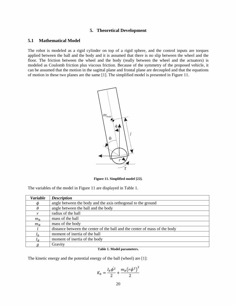
The robot is modeled as a rigid cylinder on top of a rigid sphere, and the control inputs are torques
applied between the ball and the body and it is assumed that there is no slip between the wheel and the
floor. The friction between the wheel and the body (really between the wheel and the actuators) is
modeled as Coulomb friction plus viscous friction. Because of the symmetry of the proposed vehicle, it
can be assumed that the motion in the sagittal plane and frontal plane are decoupled and that the equations
of motion in these two planes are the same [1]. The simplified model is presented in Figure 11.
Figure 11. Simplified model [22].
The variables of the model in Figure 11 are displayed in Table 1.
Variable Description
angle between the body and the axis orthogonal to the ground
angle between the ball and the body
radius of the ball
mass of the ball
mass of the body
distance between the center of the ball and the center of mass of the body
moment of inertia of the ball
moment of inertia of the body
Gravity Table 1. Model parameters.
The kinetic energy and the potential energy of the ball (wheel) are [1]:
( )

21
The kinetic energy and the potential energy of the body are [1]:
( ( ) ( )
)
( )
As mention before, the non-conservative forces are modeled as a Coulomb friction plus viscous friction
[21]:
( )
where is the Coulomb friction and is the viscous damping friction coefficient between the ball and
the actuators (Figure 12).
Figure 12. Complete friction model.
The generalized coordinate vector of the system is defined as [ ] . The Euler-Lagrange equations
of motion for the simplified planar model are:
(
)
[
] [
( )
]
where is the Lagrangian and is the torque applied between the ball and the body in the direction
normal to the plane.
The differential equations that are derived from the Lagrangian approach are:
( (
) ( ( ) )) ( ( ( )) )
( )
( )( ( ) ) ( )
22
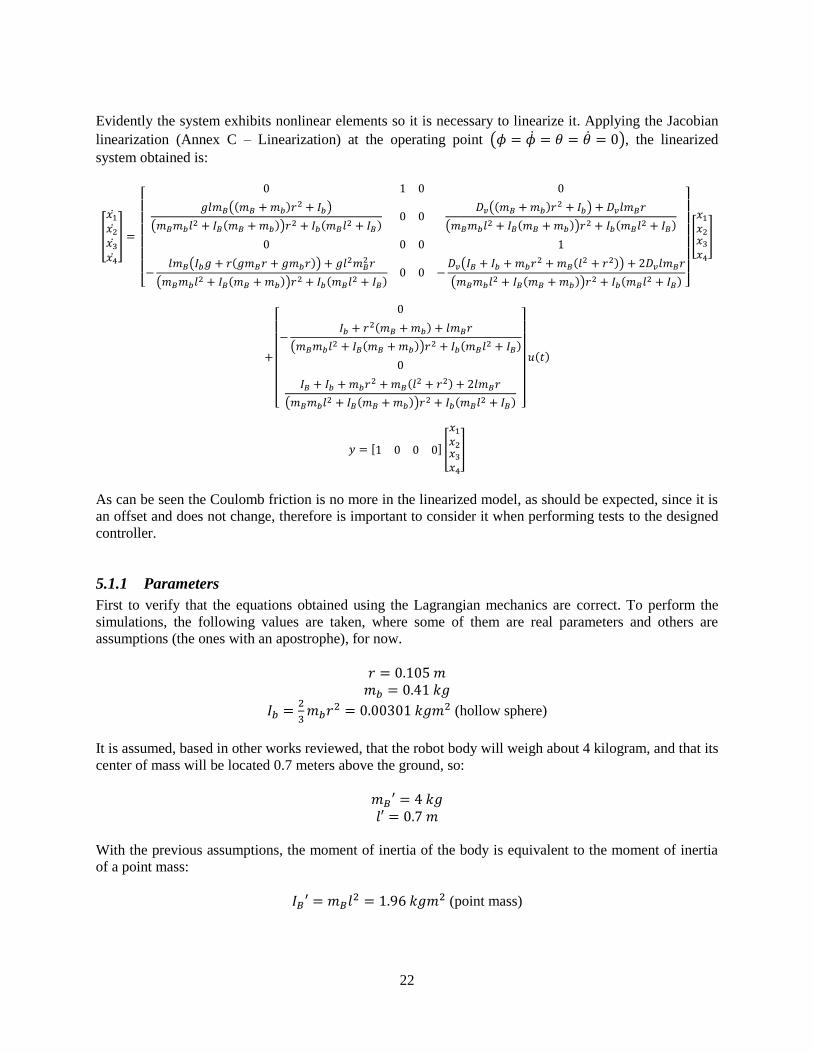
Evidently the system exhibits nonlinear elements so it is necessary to linearize it. Applying the Jacobian
linearization (Annex C – Linearization) at the operating point ( ), the linearized
system obtained is:
[
]
[
( )
( )
(
)
( )
( )
( )
(
)
( )
]
[
]
[
( )
( )
]
[ ] [
]
As can be seen the Coulomb friction is no more in the linearized model, as should be expected, since it is
an offset and does not change, therefore is important to consider it when performing tests to the designed
controller.
5.1.1 Parameters
First to verify that the equations obtained using the Lagrangian mechanics are correct. To perform the
simulations, the following values are taken, where some of them are real parameters and others are
assumptions (the ones with an apostrophe), for now.
(hollow sphere)
It is assumed, based in other works reviewed, that the robot body will weigh about 4 kilogram, and that its
center of mass will be located 0.7 meters above the ground, so:
With the previous assumptions, the moment of inertia of the body is equivalent to the moment of inertia
of a point mass:
(point mass)
23
To have a reasonable value for the viscous damping friction coefficient , from [22] is taken the 10
percent the value there since the friction of the robot Ballbot is considerably larger because of its
configuration, so:
To determine the Coulomb friction of the system, it was decided to take a different approach, for
simplicity, than the one presented in [1]. In this paper the Coulomb friction is included in the robot model
as mentioned in the previous section, and in [22] its value is determined with some experimental setup. In
this work the Coulomb friction is included directly in the actuators that drive the spherical wheel, so the
plant itself does not have this kind of friction ( ). In section 5.2 is discussed the modeling and
determination of the Coulomb friction in the actuators.
With the selected parameters now can be verified whether the differential equations derived from the
Lagrange approach truly represent the dynamics of the system. A simple way to prove this is by checking
the equilibrium points of the system and its dynamical behavior in open-loop.
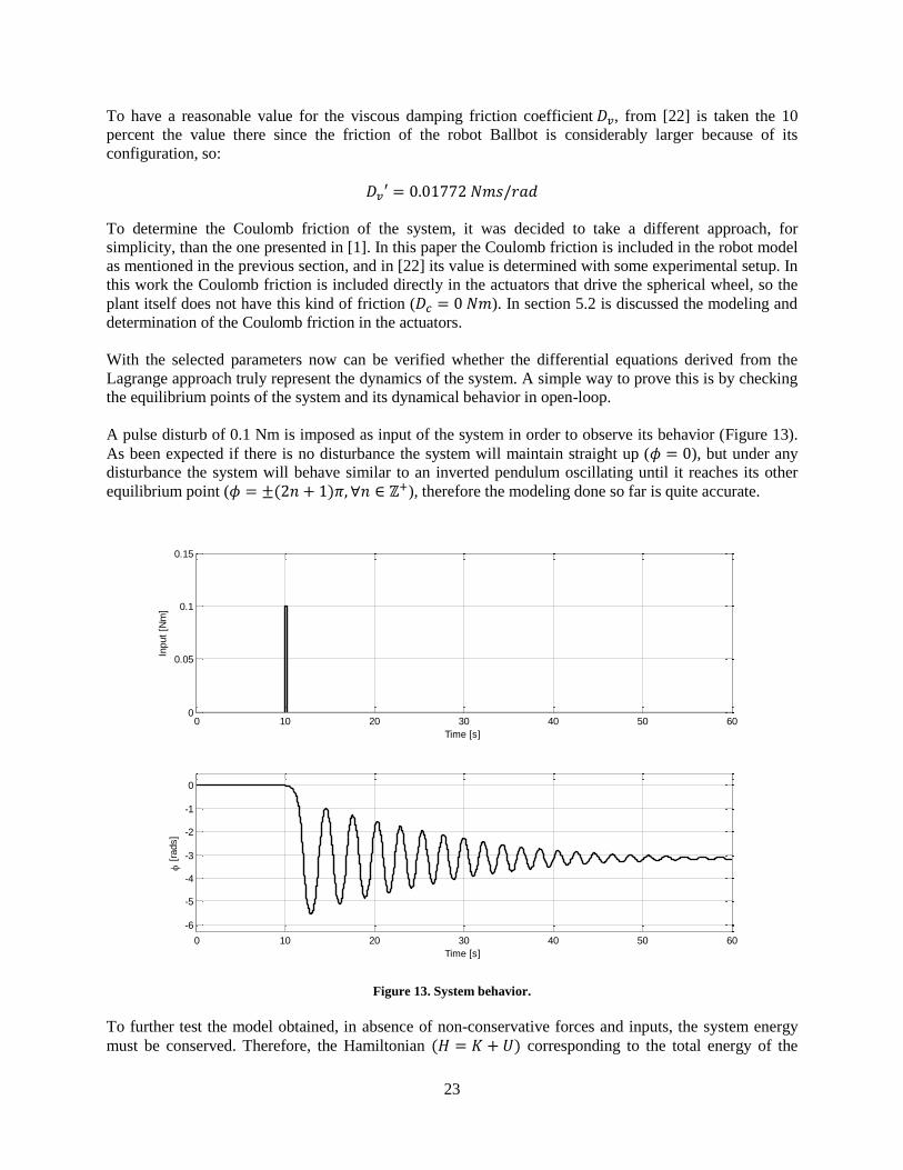
A pulse disturb of 0.1 Nm is imposed as input of the system in order to observe its behavior (Figure 13).
As been expected if there is no disturbance the system will maintain straight up ( ), but under any
disturbance the system will behave similar to an inverted pendulum oscillating until it reaches its other
equilibrium point ( ), therefore the modeling done so far is quite accurate.
Figure 13. System behavior.
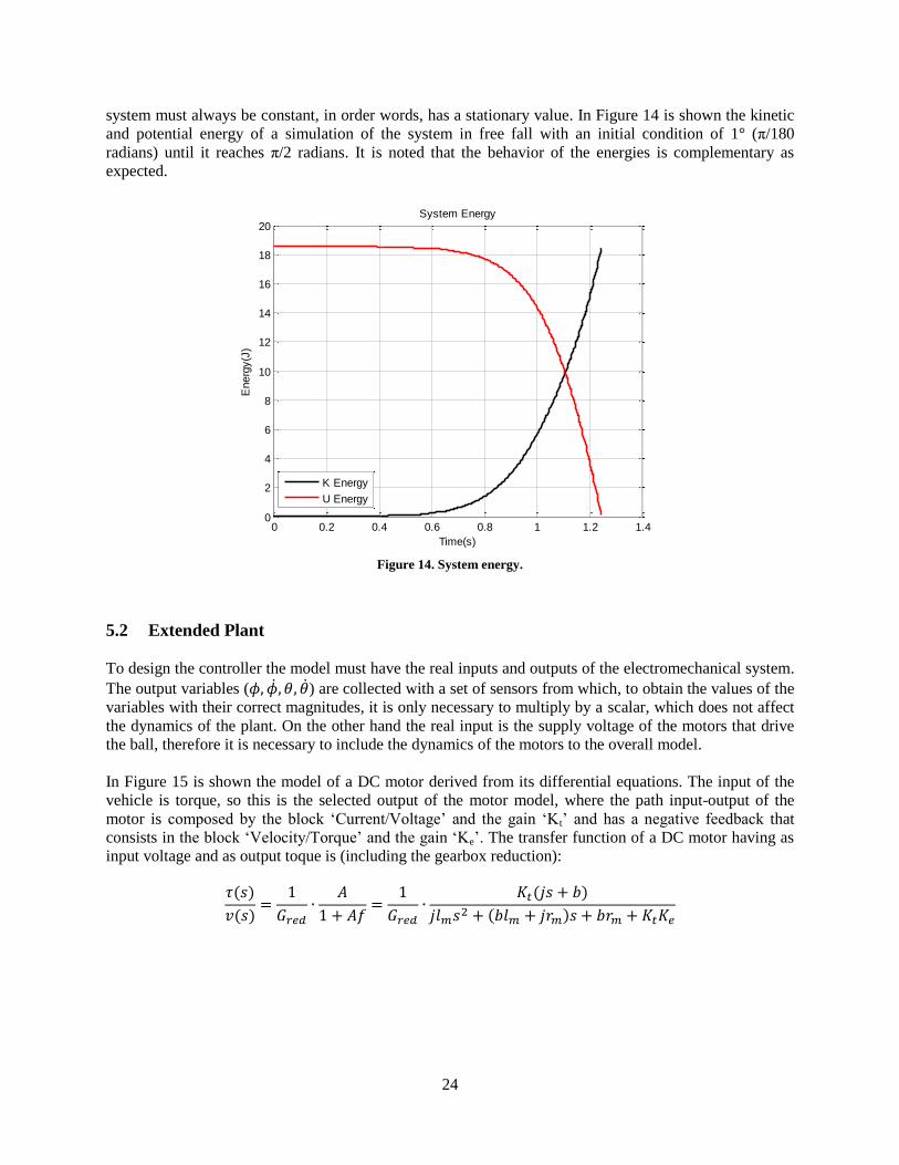
To further test the model obtained, in absence of non-conservative forces and inputs, the system energy
must be conserved. Therefore, the Hamiltonian corresponding to the total energy of the
0 10 20 30 40 50 600
0.05
0.1
0.15
Time [s]
Input
[Nm
]
0 10 20 30 40 50 60
-6
-5
-4
-3
-2
-1
0
Time [s]
[
rads]
24
system must always be constant, in order words, has a stationary value. In Figure 14 is shown the kinetic
and potential energy of a simulation of the system in free fall with an initial condition of 1° (π/180
radians) until it reaches π/2 radians. It is noted that the behavior of the energies is complementary as
expected.
Figure 14. System energy.
5.2 Extended Plant
To design the controller the model must have the real inputs and outputs of the electromechanical system.
The output variables ( ) are collected with a set of sensors from which, to obtain the values of the
variables with their correct magnitudes, it is only necessary to multiply by a scalar, which does not affect
the dynamics of the plant. On the other hand the real input is the supply voltage of the motors that drive
the ball, therefore it is necessary to include the dynamics of the motors to the overall model.
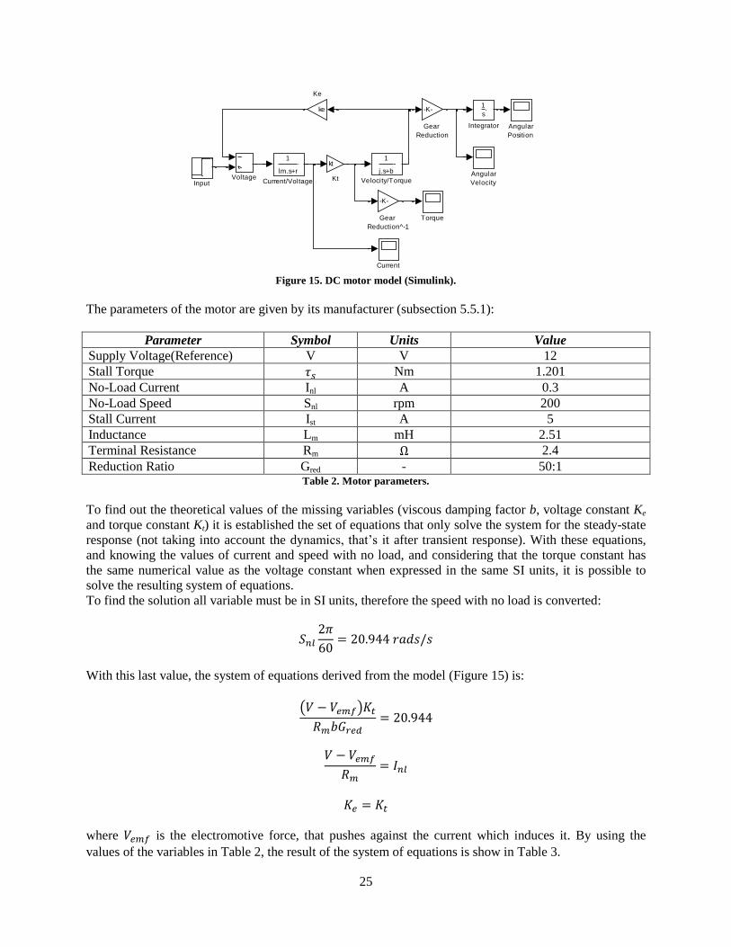
In Figure 15 is shown the model of a DC motor derived from its differential equations. The input of the
vehicle is torque, so this is the selected output of the motor model, where the path input-output of the
motor is composed by the block ‘Current/Voltage’ and the gain ‘Kt’ and has a negative feedback that
consists in the block ‘Velocity/Torque’ and the gain ‘Ke’. The transfer function of a DC motor having as
input voltage and as output toque is (including the gearbox reduction):
0 0.2 0.4 0.6 0.8 1 1.2 1.40
2
4
6
8
10
12
14
16
18
20System Energy
Time(s)
Energ
y(J
)
K Energy
U Energy
25
Figure 15. DC motor model (Simulink).
The parameters of the motor are given by its manufacturer (subsection 5.5.1):
Parameter Symbol Units Value
Supply Voltage(Reference) V V 12
Stall Torque Nm 1.201
No-Load Current Inl A 0.3
No-Load Speed Snl rpm 200
Stall Current Ist A 5
Inductance Lm mH 2.51
Terminal Resistance Rm 2.4
Reduction Ratio Gred - 50:1 Table 2. Motor parameters.
To find out the theoretical values of the missing variables (viscous damping factor b, voltage constant Ke
and torque constant Kt) it is established the set of equations that only solve the system for the steady-state
response (not taking into account the dynamics, that’s it after transient response). With these equations,
and knowing the values of current and speed with no load, and considering that the torque constant has
the same numerical value as the voltage constant when expressed in the same SI units, it is possible to
solve the resulting system of equations.
To find the solution all variable must be in SI units, therefore the speed with no load is converted:
With this last value, the system of equations derived from the model (Figure 15) is:
( )
where is the electromotive force, that pushes against the current which induces it. By using the
values of the variables in Table 2, the result of the system of equations is show in Table 3.
Voltage
1
j.s+b
Velocity/Torque
Torque
kt
Kt
ke
Ke
1
s
Integrator
Input
-K-
Gear
Reduction^-1
-K-
Gear
Reduction
1
lm.s+r
Current/Voltage
Current
Angular
Velocity
Angular
Position
26
Parameter Symbol Units Value
Torque Constant Kt Nm/A 0.010746
Voltage Constant Ke V s/rad 0.010746
Viscous Damping Factor B Nm s/rad 3.071142 10-6
Table 3. Missing motor parameters.
To find out a fair value of the inertia of the motor, it has to be considered the motor rotor and the load.
A similar motor [33] with the same nominal supply voltage, and very similar parameters, was chosen
from the manufacturer Pittman® from which its value of rotor inertia is employed (2.05 µKgm2). On the
other hand, every motor has attached to the gearbox shaft a holonomic wheel, with a diameter of 69.9 mm
and a mass of 33.6 grams (subsection 5.5.3), that could be considered as a solid cylinder, so the inertia of
this load, is:
The load inertia reflected back to the motor is a squared function of the ratio, thus:
The inertia of the holonomic wheel can be neglected, so the total inertia is just the inertia of the motor
rotor:
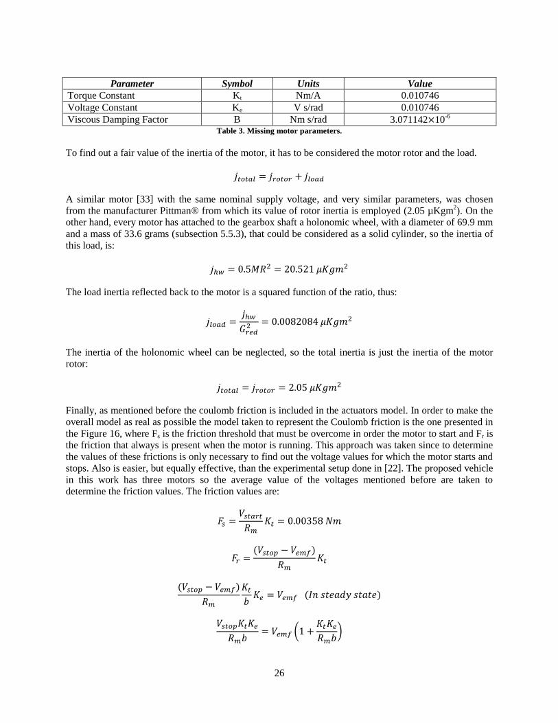
Finally, as mentioned before the coulomb friction is included in the actuators model. In order to make the
overall model as real as possible the model taken to represent the Coulomb friction is the one presented in
the Figure 16, where Fs is the friction threshold that must be overcome in order the motor to start and Fr is
the friction that always is present when the motor is running. This approach was taken since to determine
the values of these frictions is only necessary to find out the voltage values for which the motor starts and
stops. Also is easier, but equally effective, than the experimental setup done in [22]. The proposed vehicle
in this work has three motors so the average value of the voltages mentioned before are taken to
determine the friction values. The friction values are:
(
)
27
Figure 16. Motor friction model.
This way the complete model of a motor is the one presented in the Figure 17. It is to be noted that these
frictions must be included in the model before the gear reduction gain.
Figure 17. DC motor complete model (Simulink).
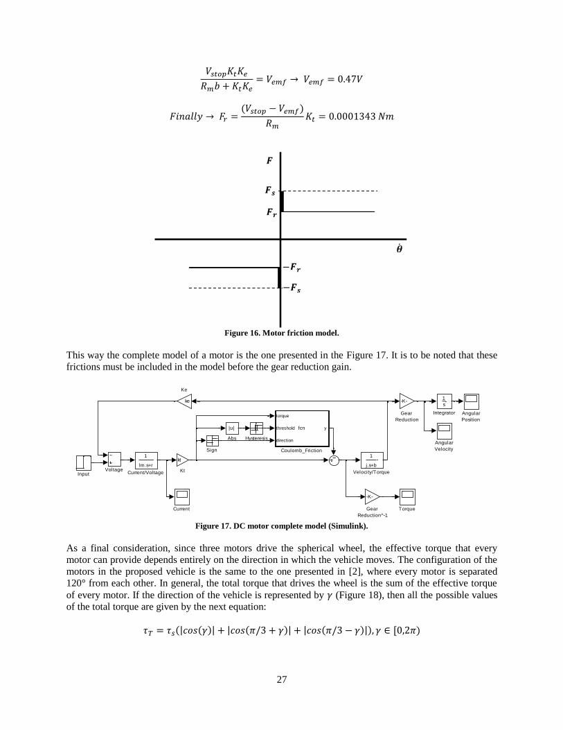
As a final consideration, since three motors drive the spherical wheel, the effective torque that every
motor can provide depends entirely on the direction in which the vehicle moves. The configuration of the
motors in the proposed vehicle is the same to the one presented in [2], where every motor is separated
120° from each other. In general, the total torque that drives the wheel is the sum of the effective torque
of every motor. If the direction of the vehicle is represented by (Figure 18), then all the possible values
of the total torque are given by the next equation:
[
Voltage
1
j.s+b
Velocity/Torque
Torque
Sign
kt
Kt
ke
Ke
1
s
Integrator
Input
Hysteresis
-K-
Gear
Reduction^-1
-K-
Gear
Reduction
1
lm.s+r
Current/Voltage
Current
torque
threshold
direction
yfcn
Coulomb_Friction
Angular
Velocity
Angular
Position
|u|
Abs
28
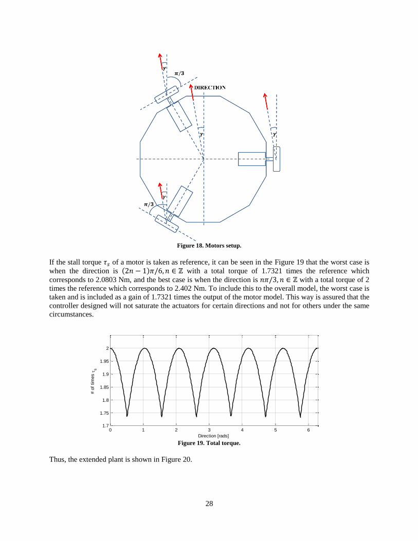
Figure 18. Motors setup.
If the stall torque of a motor is taken as reference, it can be seen in the Figure 19 that the worst case is
when the direction is with a total torque of 1.7321 times the reference which
corresponds to 2.0803 Nm, and the best case is when the direction is with a total torque of 2
times the reference which corresponds to 2.402 Nm. To include this to the overall model, the worst case is
taken and is included as a gain of 1.7321 times the output of the motor model. This way is assured that the
controller designed will not saturate the actuators for certain directions and not for others under the same
circumstances.
Figure 19. Total torque.
Thus, the extended plant is shown in Figure 20.
0 1 2 3 4 5 61.7
1.75
1.8
1.85
1.9
1.95
2
Direction [rads]
# o
f tim
es
s

29
Figure 20. Extended plant with a controller.
5.3 Controller Design
First of all, with the preceding parameters and analysis, the minimal realizations of the transfer functions
of the motor and of the vehicle model, respectively, are:
Therefore, the transfer function of the extended plant is:
At this point of this work, the main concern is the feasibility of designing a controller capable of stabilize
the vehicle, therefore, only a controller of each type (not necessarily the best), is going to be designed.
Later on, when the real plant and actuators are properly validated, controllers with very good performance
will be designed and implemented.
5.3.1 PID Controller
A classical PID controller was designed using the computer-aided software Matlab tool sisotool. Must be
taken into account that many controllers of this kind could be obtained to stabilize the linear model, but
because of the high nonlinearity of the real system, only few actually work. Also, there are a lot of tuning
methods available, but with these is difficult, analytically, to determine the parameters of the controller,
therefore mainly a procedure of trial and error was employed [14]. Also some simple tests were included
in order to test the rejection of noise and disturbances of the controller.
From the bunch of controllers that stabilize the linear plant, to choose a single controller, is established
that the following condition must be meet:
In1 Out1
VIRTUAL MOTOR
In1 Out1
VEHICLE
0
Reference
[rads]
1.7321
Effective
Torque
In1 Out1
CONTROLLER
Motor Torque [Nm]Motor Supply [V] Vehicle Tilt [rads]
30
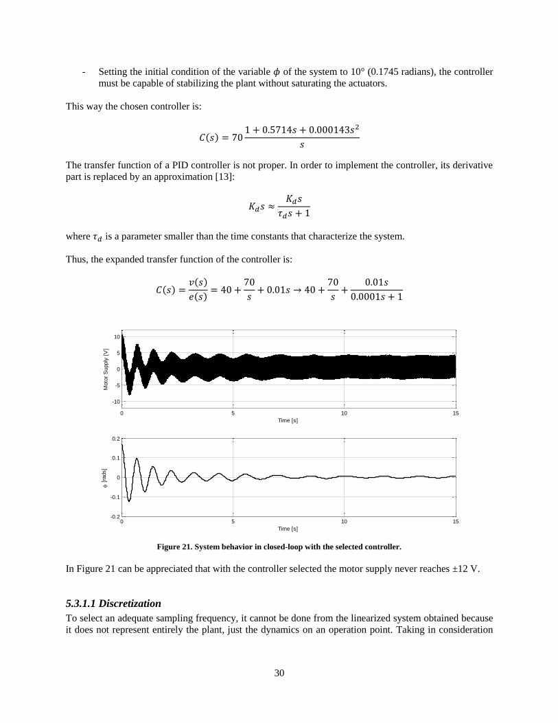
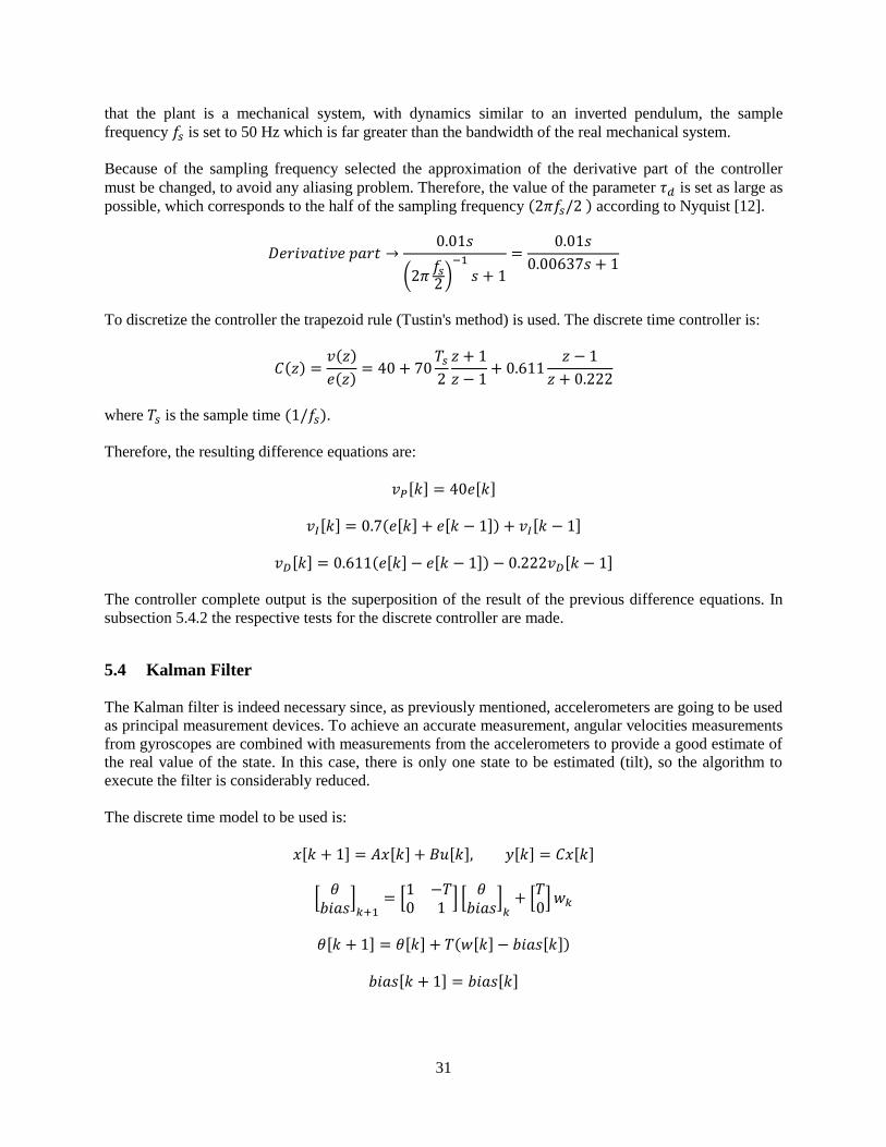
- Setting the initial condition of the variable of the system to 10° (0.1745 radians), the controller
must be capable of stabilizing the plant without saturating the actuators.
This way the chosen controller is:
The transfer function of a PID controller is not proper. In order to implement the controller, its derivative
part is replaced by an approximation [13]:
where is a parameter smaller than the time constants that characterize the system.
Thus, the expanded transfer function of the controller is:
Figure 21. System behavior in closed-loop with the selected controller.
In Figure 21 can be appreciated that with the controller selected the motor supply never reaches ±12 V.
5.3.1.1 Discretization
To select an adequate sampling frequency, it cannot be done from the linearized system obtained because
it does not represent entirely the plant, just the dynamics on an operation point. Taking in consideration
0 5 10 15
-10
-5
0
5
10
Time [s]
Moto
r S
upply
[V
]
0 5 10 15-0.2
-0.1
0
0.1
0.2
Time [s]
[
rads]
31
that the plant is a mechanical system, with dynamics similar to an inverted pendulum, the sample
frequency is set to 50 Hz which is far greater than the bandwidth of the real mechanical system.
Because of the sampling frequency selected the approximation of the derivative part of the controller
must be changed, to avoid any aliasing problem. Therefore, the value of the parameter is set as large as
possible, which corresponds to the half of the sampling frequency according to Nyquist [12].
( )
To discretize the controller the trapezoid rule (Tustin's method) is used. The discrete time controller is:
where is the sample time .
Therefore, the resulting difference equations are:
[ ] [ ]
[ ] [ ] [ ] [ ]
[ ] [ ] [ ] [ ]
The controller complete output is the superposition of the result of the previous difference equations. In
subsection 5.4.2 the respective tests for the discrete controller are made.
5.4 Kalman Filter
The Kalman filter is indeed necessary since, as previously mentioned, accelerometers are going to be used
as principal measurement devices. To achieve an accurate measurement, angular velocities measurements
from gyroscopes are combined with measurements from the accelerometers to provide a good estimate of
the real value of the state. In this case, there is only one state to be estimated (tilt), so the algorithm to
execute the filter is considerably reduced.
The discrete time model to be used is:
[ ] [ ] [ ] [ ] [ ]
[
]
[
] [
] [
]
[ ] [ ] [ ] [ ]
[ ] [ ]
32
where is the sample time, is the angular velocity, is the state (tilt), and the bias is the output level of
the gyroscope when there is no acceleration (zero velocity).
Actually, the model is just the relationship between angular velocity and angular position which is a
simple integration done through the backward rectangular method.
The bias or zero-g bias (for accelereometers) is a constant (or slowly moving offset) from the true
measurement. When good precision is needed, there are several problems concerning this bias that must
be taken into account (for both accelerometers and gyroscopes). The most relevant are [29]:
- Every time that the measurement device is turned on, there may be slight changes on the offset
value. It also depends on the quality of the power supply and its capability of maintaining an
invariant voltage.
- Temperature bias is a change in the bias of measurement devices as a function of temperature.
These devices are mainly made of silicon and temperature will expand/contract the structures
inside them.
To avoid such problems in the actual implementation (section 6.3), the following is established:
[ ]
Furthermore, last consideration minimizes the computation of the filter. The resulting system is:
[ ] [ ] [ ] [ ] [ ]
[ ] [ ] [ ] [ ] [ ]
where the matrices of the system are:
[ ] [ ] [ ]
Thus, the algorithm to be executed is reduced to:
[ ] [ ] [ ]
[ ] [ ]
[ ] [ ]( [ ] )
( [ ] )( [ ] )
[ ] [ ] [ ]( [ ] [ ]) [ ] ( [ ] [ ]) [ ] [ ]
[ ] [ ] [ ] [ ] ( [ ] )
The initial conditions are chosen as:
[ ] [ ]

33
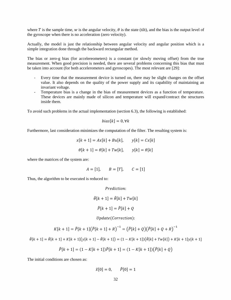
Regarding the values of and , these were experimentally obtained. Several raw measurements from
the accelerometers and gyroscopes were made simulating the vibration of the vehicle, which is the main
responsible for the noise in the signals. To get the measurements the IMU (subsection 5.5.2) was placed
horizontally over a table, which was subjected to severe shocks, while oscillatory translational
movements over the axis tested was applied to it. Actually, these shocks and oscillations exceed the real
disturbances under normal operation of the vehicle, but this way is assured that the worst case scenario is
considered in the simulations. Ten measurements (for both axes, x-axis and y-axis) were made trying to
apply shocks and oscillations with the same intensity and amplitude every time (Figure 22 and Figure 23
show one of the measurements recorded of the accelerometer and gyroscope respectively). It’s to be noted
that the value of the readings are already in the real corresponding units, that’s it radians for the
accelerometers and radians per second for the gyroscopes (subsection 6.3).
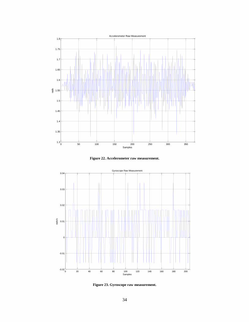
As can be seen in Figure 23, because of the low amplitude of the output of the gyroscopes under the
circumstances mention previously, the measurements recorded are not very reliable. To improve the
resolution of the reading of the gyroscopes, a low pass filter, as described in section 6.3 with a cutoff
frequency of 5 Hz, is applied to their outputs (with the sample frequency selected of 50 Hz)
[ ] [ ] [ ]
This filter does not affect the bandwidth of the signal and, this way, the filter itself computes an
interpolation of the readings achieving a more accurate signal (Figure 24).
Finally, with this last improvement, with Matlab function std the standard deviation was computed for
every measurement and then the average values were calculated (Table 4).
[rads/s] [rads]
0.00282 0.03375 Table 4. Average values of standard deviations of process and measurement noise.
{ [ ] [ ]}
{ [ ] [ ]}
34
Figure 22. Accelerometer raw measurement.
Figure 23. Gyroscope raw measurement.
0 50 100 150 200 250 300 3501.3
1.35
1.4
1.45
1.5
1.55
1.6
1.65
1.7
1.75
1.8Accelerometer Raw Measurement
Samples
rads
0 20 40 60 80 100 120 140 160 180 200-0.02
-0.01
0
0.01
0.02
0.03
0.04Gyroscope Raw Measurement
Samples
rads/s
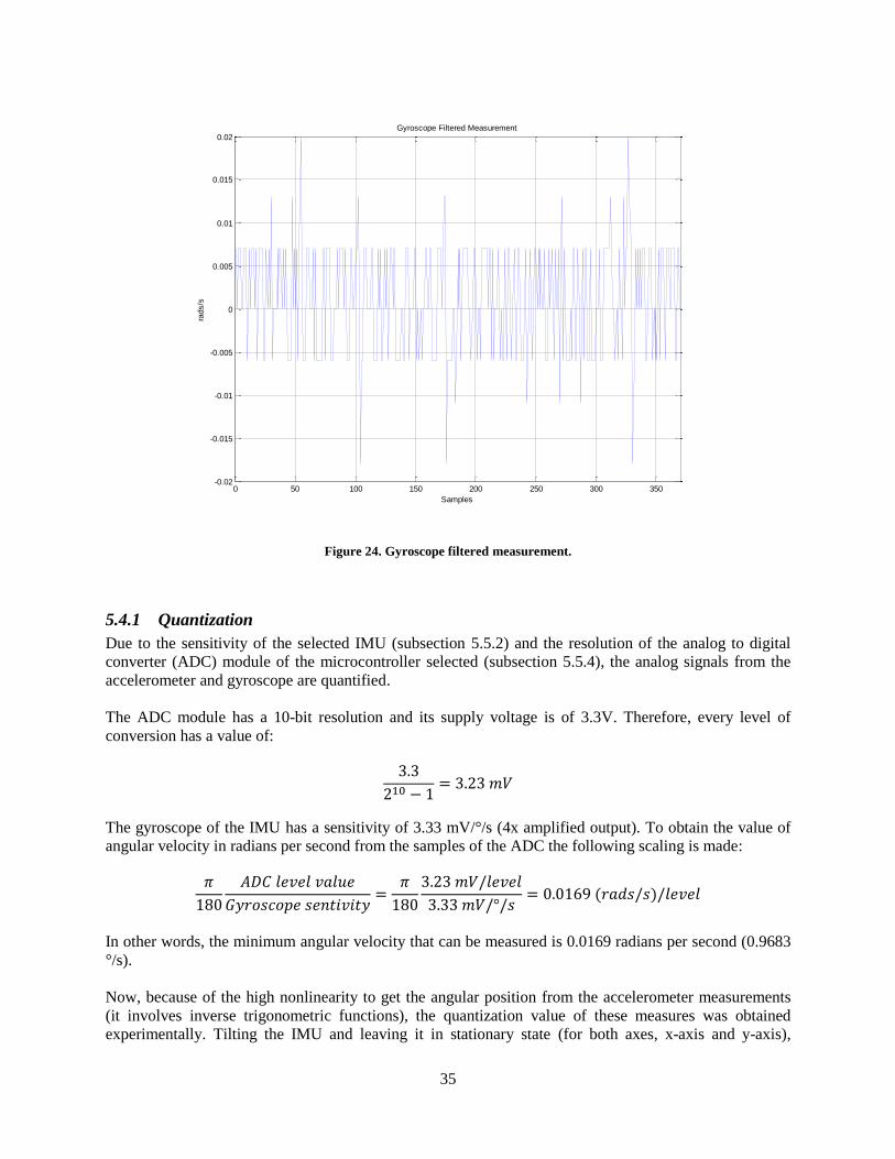
35
Figure 24. Gyroscope filtered measurement.
5.4.1 Quantization
Due to the sensitivity of the selected IMU (subsection 5.5.2) and the resolution of the analog to digital
converter (ADC) module of the microcontroller selected (subsection 5.5.4), the analog signals from the
accelerometer and gyroscope are quantified.
The ADC module has a 10-bit resolution and its supply voltage is of 3.3V. Therefore, every level of
conversion has a value of:
The gyroscope of the IMU has a sensitivity of 3.33 mV/°/s (4x amplified output). To obtain the value of
angular velocity in radians per second from the samples of the ADC the following scaling is made:
In other words, the minimum angular velocity that can be measured is 0.0169 radians per second (0.9683
°/s).
Now, because of the high nonlinearity to get the angular position from the accelerometer measurements
(it involves inverse trigonometric functions), the quantization value of these measures was obtained
experimentally. Tilting the IMU and leaving it in stationary state (for both axes, x-axis and y-axis),
0 50 100 150 200 250 300 350-0.02
-0.015
-0.01
-0.005
0
0.005
0.01
0.015
0.02Gyroscope Filtered Measurement
Samples
rads/s
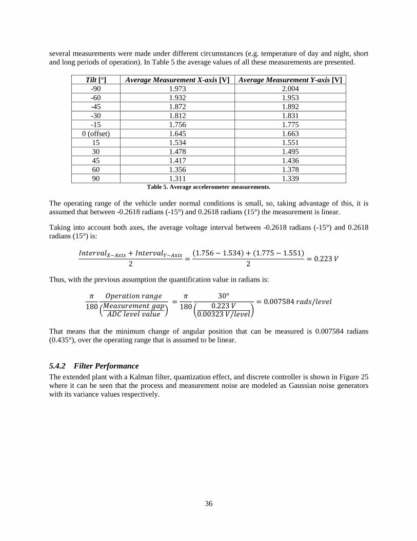
36
several measurements were made under different circumstances (e.g. temperature of day and night, short
and long periods of operation). In Table 5 the average values of all these measurements are presented.
Tilt [°] Average Measurement X-axis [V] Average Measurement Y-axis [V]
-90 1.973 2.004
-60 1.932 1.953
-45 1.872 1.892
-30 1.812 1.831
-15 1.756 1.775
0 (offset) 1.645 1.663
15 1.534 1.551
30 1.478 1.495
45 1.417 1.436
60 1.356 1.378
90 1.311 1.339 Table 5. Average accelerometer measurements.
The operating range of the vehicle under normal conditions is small, so, taking advantage of this, it is
assumed that between -0.2618 radians (-15°) and 0.2618 radians (15°) the measurement is linear.
Taking into account both axes, the average voltage interval between -0.2618 radians (-15°) and 0.2618
radians (15°) is:
Thus, with the previous assumption the quantification value in radians is:
(
)
(
)
That means that the minimum change of angular position that can be measured is 0.007584 radians
(0.435°), over the operating range that is assumed to be linear.
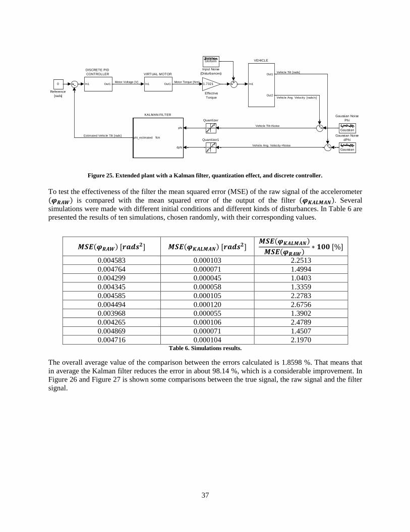
5.4.2 Filter Performance
The extended plant with a Kalman filter, quantization effect, and discrete controller is shown in Figure 25
where it can be seen that the process and measurement noise are modeled as Gaussian noise generators
with its variance values respectively.
37
Figure 25. Extended plant with a Kalman filter, quantization effect, and discrete controller.
To test the effectiveness of the filter the mean squared error (MSE) of the raw signal of the accelerometer
is compared with the mean squared error of the output of the filter . Several
simulations were made with different initial conditions and different kinds of disturbances. In Table 6 are
presented the results of ten simulations, chosen randomly, with their corresponding values.
[ ] [ ]
[ ]
0.004583 0.000103 2.2513
0.004764 0.000071 1.4994
0.004299 0.000045 1.0403
0.004345 0.000058 1.3359
0.004585 0.000105 2.2783
0.004494 0.000120 2.6756
0.003968 0.000055 1.3902
0.004265 0.000106 2.4789
0.004869 0.000071 1.4507
0.004716 0.000104 2.1970 Table 6. Simulations results.
The overall average value of the comparison between the errors calculated is 1.8598 %. That means that
in average the Kalman filter reduces the error in about 98.14 %, which is a considerable improvement. In
Figure 26 and Figure 27 is shown some comparisons between the true signal, the raw signal and the filter
signal.
In1 Out1
VIRTUAL MOTOR
In1
Out1
Out2
VEHICLE
0
Reference
[rads]
Quantizer1
Quantizer
phi
dphi
phi_estimated fcn
KALMAN FILTER
Uniform
Input Noise
(Disturbances)
Gaussian
Gaussian Noise
dPhi
Gaussian
Gaussian Noise
Phi
1.7321
Effective
Torque
In1 Out1
DISCRETE PID
CONTROLLER
Vehicle Ang. Velocity +Noise
Vehicle Tilt+Noise
Motor Torque [Nm]Motor Voltage [V]
Vehicle Tilt [rads]
Estimated Vehicle Tilt [rads]
Vehicle Ang. Velocity [rads/s]
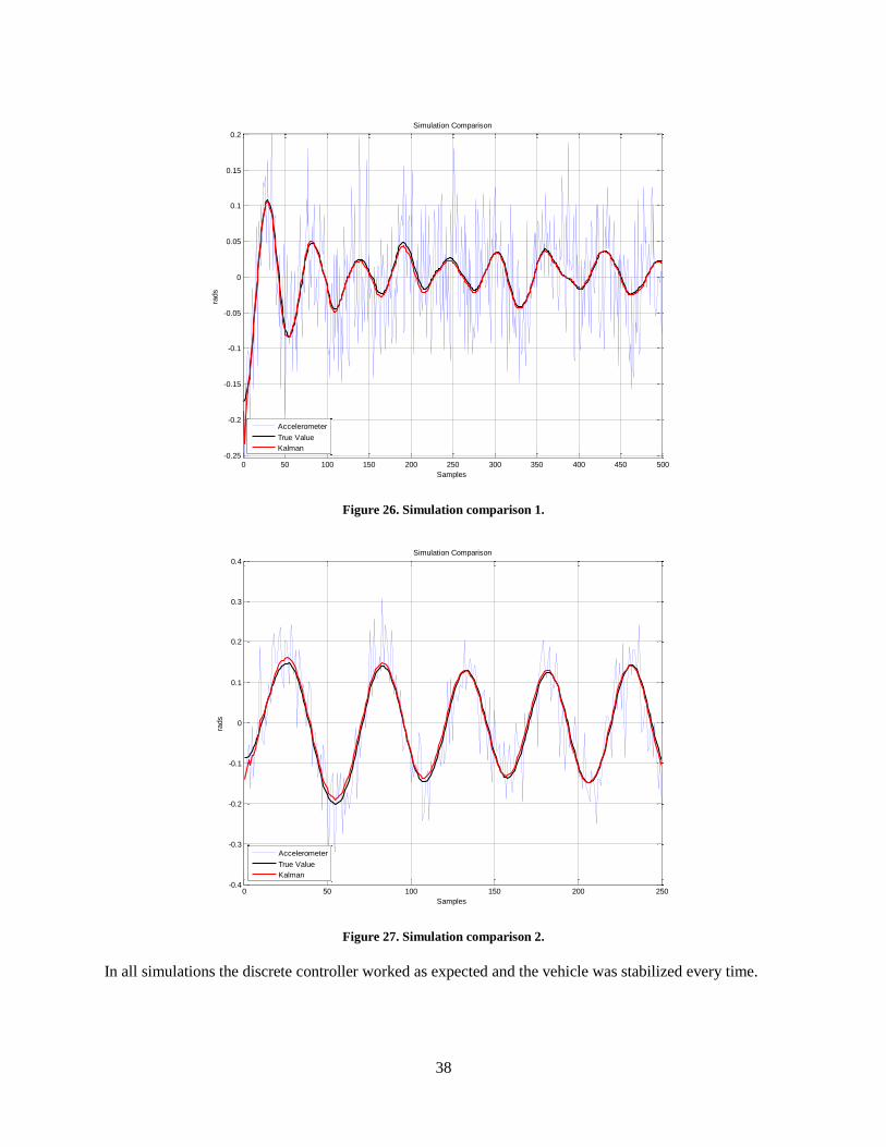
38
Figure 26. Simulation comparison 1.
Figure 27. Simulation comparison 2.
In all simulations the discrete controller worked as expected and the vehicle was stabilized every time.
0 50 100 150 200 250 300 350 400 450 500-0.25
-0.2
-0.15
-0.1
-0.05
0
0.05
0.1
0.15
0.2
Simulation Comparison
Samples
rads
Accelerometer
True Value
Kalman
0 50 100 150 200 250-0.4
-0.3
-0.2
-0.1
0
0.1
0.2
0.3
0.4Simulation Comparison
Samples
rads
Accelerometer
True Value
Kalman
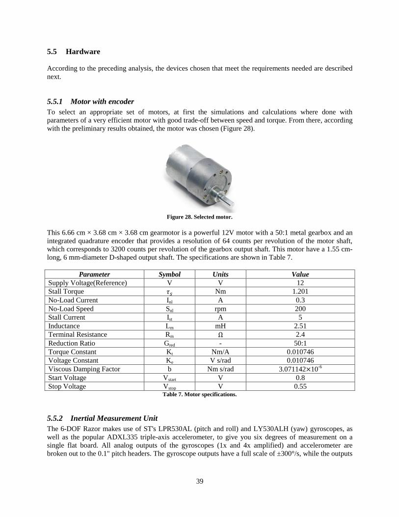
39
5.5 Hardware
According to the preceding analysis, the devices chosen that meet the requirements needed are described
next.
5.5.1 Motor with encoder
To select an appropriate set of motors, at first the simulations and calculations where done with
parameters of a very efficient motor with good trade-off between speed and torque. From there, according
with the preliminary results obtained, the motor was chosen (Figure 28).
Figure 28. Selected motor.
This 6.66 cm × 3.68 cm × 3.68 cm gearmotor is a powerful 12V motor with a 50:1 metal gearbox and an
integrated quadrature encoder that provides a resolution of 64 counts per revolution of the motor shaft,
which corresponds to 3200 counts per revolution of the gearbox output shaft. This motor have a 1.55 cm-
long, 6 mm-diameter D-shaped output shaft. The specifications are shown in Table 7.
Parameter Symbol Units Value
Supply Voltage(Reference) V V 12
Stall Torque Nm 1.201
No-Load Current Inl A 0.3
No-Load Speed Snl rpm 200
Stall Current Ist A 5
Inductance Lm mH 2.51
Terminal Resistance Rm 2.4
Reduction Ratio Gred - 50:1
Torque Constant Kt Nm/A 0.010746
Voltage Constant Ke V s/rad 0.010746
Viscous Damping Factor b Nm s/rad 3.071142 10-6
Start Voltage Vstart V 0.8
Stop Voltage Vstop V 0.55 Table 7. Motor specifications.
5.5.2 Inertial Measurement Unit
The 6-DOF Razor makes use of ST's LPR530AL (pitch and roll) and LY530ALH (yaw) gyroscopes, as
well as the popular ADXL335 triple-axis accelerometer, to give you six degrees of measurement on a
single flat board. All analog outputs of the gyroscopes (1x and 4x amplified) and accelerometer are
broken out to the 0.1" pitch headers. The gyroscope outputs have a full scale of ±300°/s, while the outputs
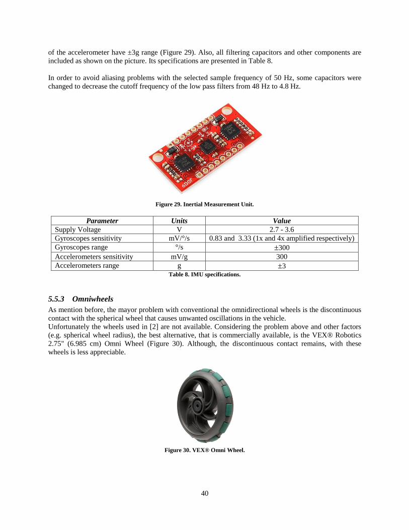
40
of the accelerometer have ±3g range (Figure 29). Also, all filtering capacitors and other components are
included as shown on the picture. Its specifications are presented in Table 8.
In order to avoid aliasing problems with the selected sample frequency of 50 Hz, some capacitors were
changed to decrease the cutoff frequency of the low pass filters from 48 Hz to 4.8 Hz.
Figure 29. Inertial Measurement Unit.
Parameter Units Value
Supply Voltage V 2.7 - 3.6
Gyroscopes sensitivity mV/°/s 0.83 and 3.33 (1x and 4x amplified respectively)
Gyroscopes range °/s ±300
Accelerometers sensitivity mV/g 300
Accelerometers range g ±3 Table 8. IMU specifications.
5.5.3 Omniwheels
As mention before, the mayor problem with conventional the omnidirectional wheels is the discontinuous
contact with the spherical wheel that causes unwanted oscillations in the vehicle.
Unfortunately the wheels used in [2] are not available. Considering the problem above and other factors
(e.g. spherical wheel radius), the best alternative, that is commercially available, is the VEX® Robotics
2.75" (6.985 cm) Omni Wheel (Figure 30). Although, the discontinuous contact remains, with these
wheels is less appreciable.
Figure 30. VEX® Omni Wheel.
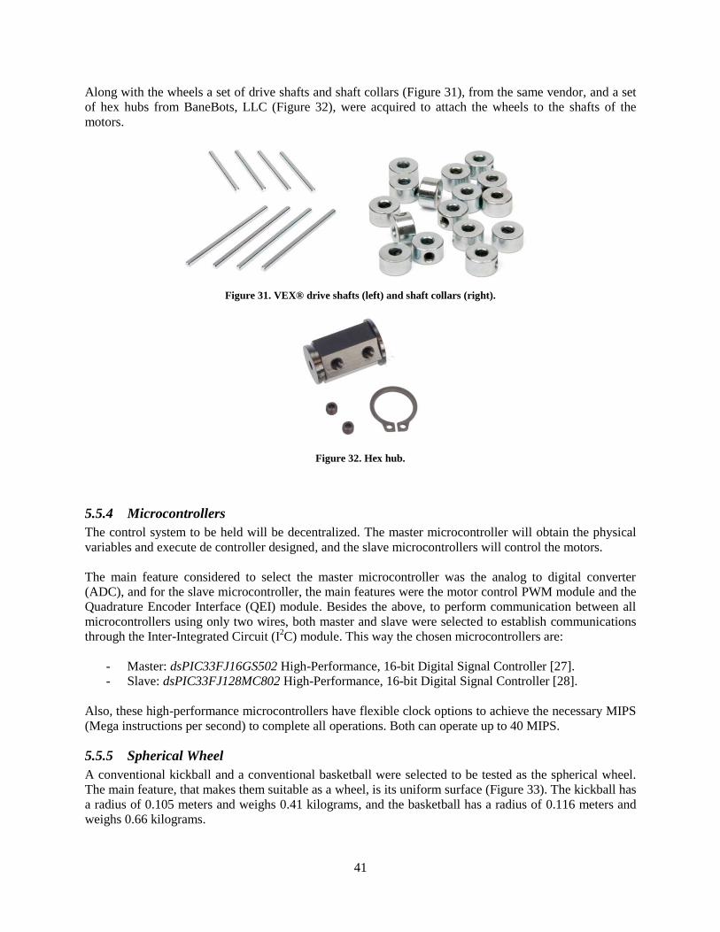
41
Along with the wheels a set of drive shafts and shaft collars (Figure 31), from the same vendor, and a set
of hex hubs from BaneBots, LLC (Figure 32), were acquired to attach the wheels to the shafts of the
motors.
Figure 31. VEX® drive shafts (left) and shaft collars (right).
Figure 32. Hex hub.
5.5.4 Microcontrollers
The control system to be held will be decentralized. The master microcontroller will obtain the physical
variables and execute de controller designed, and the slave microcontrollers will control the motors.
The main feature considered to select the master microcontroller was the analog to digital converter
(ADC), and for the slave microcontroller, the main features were the motor control PWM module and the
Quadrature Encoder Interface (QEI) module. Besides the above, to perform communication between all
microcontrollers using only two wires, both master and slave were selected to establish communications
through the Inter-Integrated Circuit (I2C) module. This way the chosen microcontrollers are:
- Master: dsPIC33FJ16GS502 High-Performance, 16-bit Digital Signal Controller [27].
- Slave: dsPIC33FJ128MC802 High-Performance, 16-bit Digital Signal Controller [28].
Also, these high-performance microcontrollers have flexible clock options to achieve the necessary MIPS
(Mega instructions per second) to complete all operations. Both can operate up to 40 MIPS.
5.5.5 Spherical Wheel
A conventional kickball and a conventional basketball were selected to be tested as the spherical wheel.
The main feature, that makes them suitable as a wheel, is its uniform surface (Figure 33). The kickball has
a radius of 0.105 meters and weighs 0.41 kilograms, and the basketball has a radius of 0.116 meters and
weighs 0.66 kilograms.
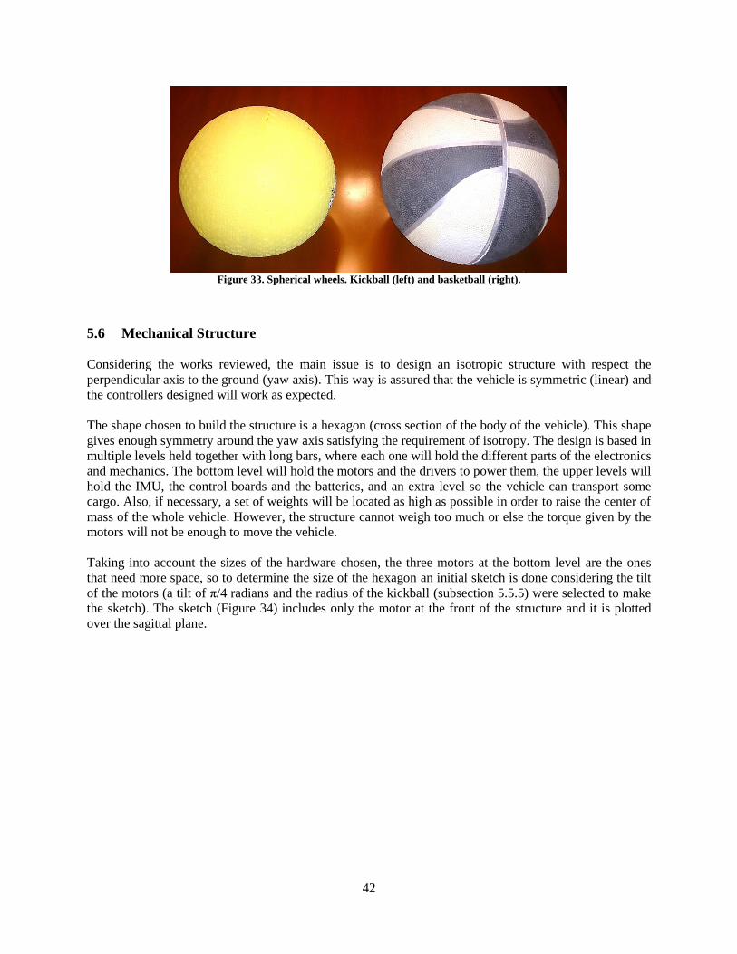
42
Figure 33. Spherical wheels. Kickball (left) and basketball (right).
5.6 Mechanical Structure
Considering the works reviewed, the main issue is to design an isotropic structure with respect the
perpendicular axis to the ground (yaw axis). This way is assured that the vehicle is symmetric (linear) and
the controllers designed will work as expected.
The shape chosen to build the structure is a hexagon (cross section of the body of the vehicle). This shape
gives enough symmetry around the yaw axis satisfying the requirement of isotropy. The design is based in
multiple levels held together with long bars, where each one will hold the different parts of the electronics
and mechanics. The bottom level will hold the motors and the drivers to power them, the upper levels will
hold the IMU, the control boards and the batteries, and an extra level so the vehicle can transport some
cargo. Also, if necessary, a set of weights will be located as high as possible in order to raise the center of
mass of the whole vehicle. However, the structure cannot weigh too much or else the torque given by the
motors will not be enough to move the vehicle.
Taking into account the sizes of the hardware chosen, the three motors at the bottom level are the ones
that need more space, so to determine the size of the hexagon an initial sketch is done considering the tilt
of the motors (a tilt of π/4 radians and the radius of the kickball (subsection 5.5.5) were selected to make
the sketch). The sketch (Figure 34) includes only the motor at the front of the structure and it is plotted
over the sagittal plane.
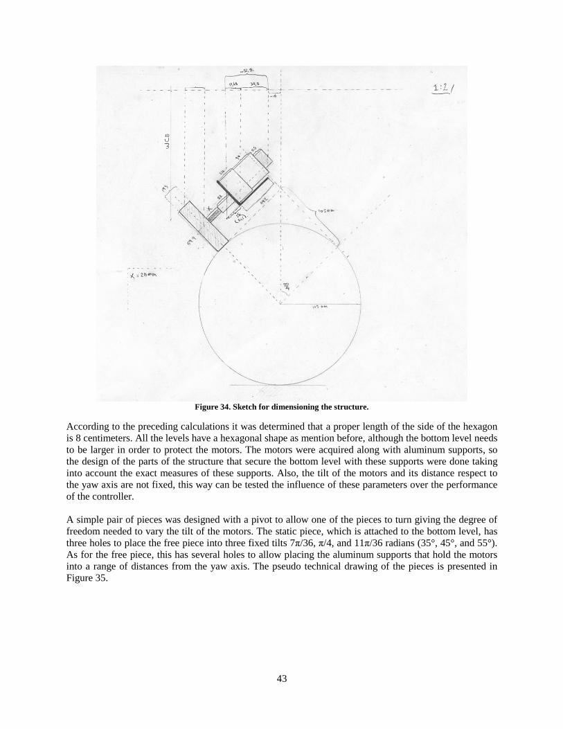
43
Figure 34. Sketch for dimensioning the structure.
According to the preceding calculations it was determined that a proper length of the side of the hexagon
is 8 centimeters. All the levels have a hexagonal shape as mention before, although the bottom level needs
to be larger in order to protect the motors. The motors were acquired along with aluminum supports, so
the design of the parts of the structure that secure the bottom level with these supports were done taking
into account the exact measures of these supports. Also, the tilt of the motors and its distance respect to
the yaw axis are not fixed, this way can be tested the influence of these parameters over the performance
of the controller.
A simple pair of pieces was designed with a pivot to allow one of the pieces to turn giving the degree of
freedom needed to vary the tilt of the motors. The static piece, which is attached to the bottom level, has
three holes to place the free piece into three fixed tilts 7π/36, π/4, and 11π/36 radians (35°, 45°, and 55°).
As for the free piece, this has several holes to allow placing the aluminum supports that hold the motors
into a range of distances from the yaw axis. The pseudo technical drawing of the pieces is presented in
Figure 35.
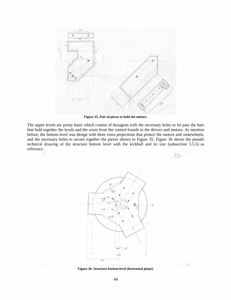
44
Figure 35. Pair of pieces to hold the motors.
The upper levels are pretty basic which consist of hexagons with the necessary holes to let pass the bars
that hold together the levels and the wires from the control boards to the drivers and motors. As mention
before, the bottom level was design with three extra projections that protect the motors and omniwheels,
and the necessary holes to secure together the pieces shown in Figure 35. Figure 36 shows the pseudo
technical drawing of the structure bottom level with the kickball and its size (subsection 5.5.5) as
reference.
Figure 36. Structure bottom level (horizontal plane).
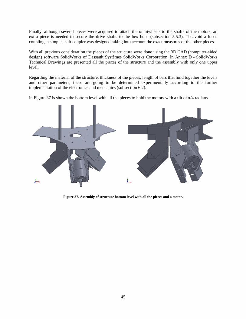
45
Finally, although several pieces were acquired to attach the omniwheels to the shafts of the motors, an
extra piece is needed to secure the drive shafts to the hex hubs (subsection 5.5.3). To avoid a loose
coupling, a simple shaft coupler was designed taking into account the exact measures of the other pieces.
With all previous consideration the pieces of the structure were done using the 3D CAD (computer-aided
design) software SolidWorks of Dassault Systèmes SolidWorks Corporation. In Annex D - SolidWorks
Technical Drawings are presented all the pieces of the structure and the assembly with only one upper
level.
Regarding the material of the structure, thickness of the pieces, length of bars that hold together the levels
and other parameters, these are going to be determined experimentally according to the further
implementation of the electronics and mechanics (subsection 6.2).
In Figure 37 is shown the bottom level with all the pieces to hold the motors with a tilt of π/4 radians.
Figure 37. Assembly of structure bottom level with all the pieces and a motor.
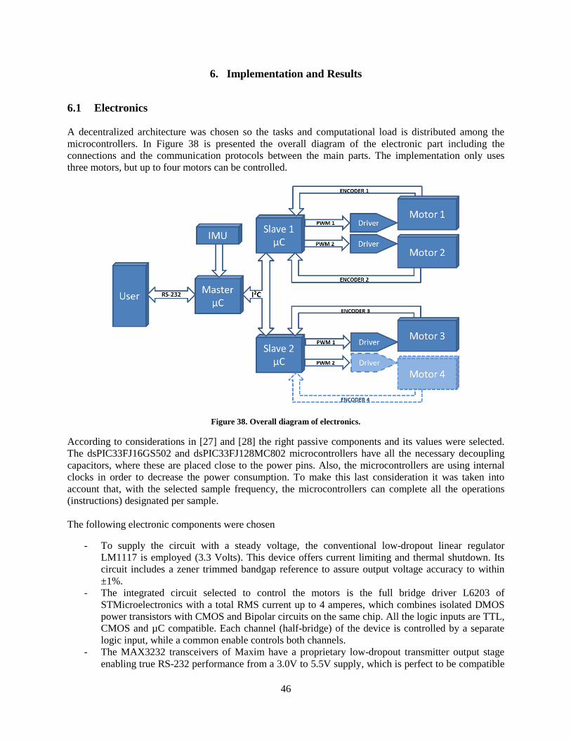
46
6. Implementation and Results
6.1 Electronics
A decentralized architecture was chosen so the tasks and computational load is distributed among the
microcontrollers. In Figure 38 is presented the overall diagram of the electronic part including the
connections and the communication protocols between the main parts. The implementation only uses
three motors, but up to four motors can be controlled.
Figure 38. Overall diagram of electronics.
According to considerations in [27] and [28] the right passive components and its values were selected.
The dsPIC33FJ16GS502 and dsPIC33FJ128MC802 microcontrollers have all the necessary decoupling
capacitors, where these are placed close to the power pins. Also, the microcontrollers are using internal
clocks in order to decrease the power consumption. To make this last consideration it was taken into
account that, with the selected sample frequency, the microcontrollers can complete all the operations
(instructions) designated per sample.
The following electronic components were chosen
- To supply the circuit with a steady voltage, the conventional low-dropout linear regulator
LM1117 is employed (3.3 Volts). This device offers current limiting and thermal shutdown. Its
circuit includes a zener trimmed bandgap reference to assure output voltage accuracy to within
±1%.
- The integrated circuit selected to control the motors is the full bridge driver L6203 of
STMicroelectronics with a total RMS current up to 4 amperes, which combines isolated DMOS
power transistors with CMOS and Bipolar circuits on the same chip. All the logic inputs are TTL,
CMOS and µC compatible. Each channel (half-bridge) of the device is controlled by a separate
logic input, while a common enable controls both channels.
- The MAX3232 transceivers of Maxim have a proprietary low-dropout transmitter output stage
enabling true RS-232 performance from a 3.0V to 5.5V supply, which is perfect to be compatible
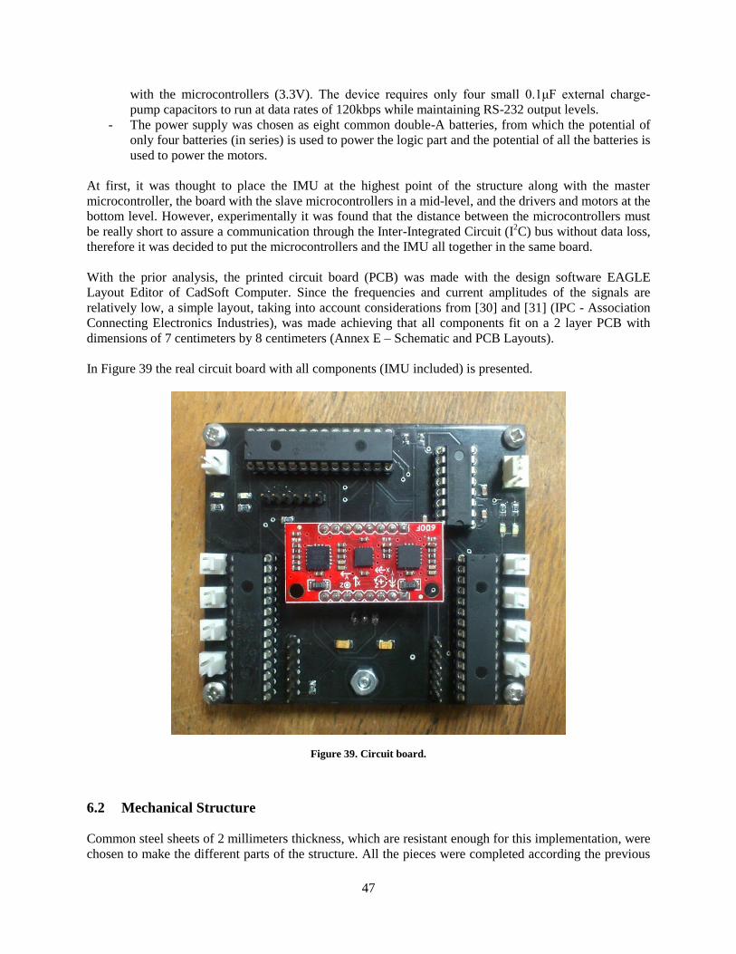
47
with the microcontrollers (3.3V). The device requires only four small 0.1μF external charge-
pump capacitors to run at data rates of 120kbps while maintaining RS-232 output levels.
- The power supply was chosen as eight common double-A batteries, from which the potential of
only four batteries (in series) is used to power the logic part and the potential of all the batteries is
used to power the motors.
At first, it was thought to place the IMU at the highest point of the structure along with the master
microcontroller, the board with the slave microcontrollers in a mid-level, and the drivers and motors at the
bottom level. However, experimentally it was found that the distance between the microcontrollers must
be really short to assure a communication through the Inter-Integrated Circuit (I2C) bus without data loss,
therefore it was decided to put the microcontrollers and the IMU all together in the same board.
With the prior analysis, the printed circuit board (PCB) was made with the design software EAGLE
Layout Editor of CadSoft Computer. Since the frequencies and current amplitudes of the signals are
relatively low, a simple layout, taking into account considerations from [30] and [31] (IPC - Association
Connecting Electronics Industries), was made achieving that all components fit on a 2 layer PCB with
dimensions of 7 centimeters by 8 centimeters (Annex E – Schematic and PCB Layouts).
In Figure 39 the real circuit board with all components (IMU included) is presented.
Figure 39. Circuit board.
6.2 Mechanical Structure
Common steel sheets of 2 millimeters thickness, which are resistant enough for this implementation, were
chosen to make the different parts of the structure. All the pieces were completed according the previous
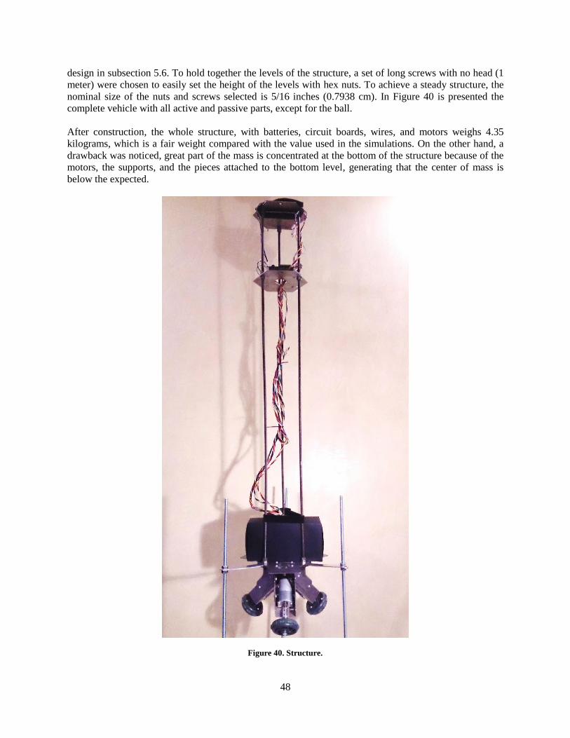
48
design in subsection 5.6. To hold together the levels of the structure, a set of long screws with no head (1
meter) were chosen to easily set the height of the levels with hex nuts. To achieve a steady structure, the
nominal size of the nuts and screws selected is 5/16 inches (0.7938 cm). In Figure 40 is presented the
complete vehicle with all active and passive parts, except for the ball.
After construction, the whole structure, with batteries, circuit boards, wires, and motors weighs 4.35
kilograms, which is a fair weight compared with the value used in the simulations. On the other hand, a
drawback was noticed, great part of the mass is concentrated at the bottom of the structure because of the
motors, the supports, and the pieces attached to the bottom level, generating that the center of mass is
below the expected.
Figure 40. Structure.
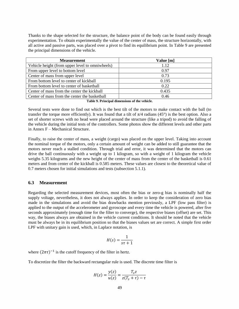
49
Thanks to the shape selected for the structure, the balance point of the body can be found easily through
experimentation. To obtain experimentally the value of the center of mass, the structure horizontally, with
all active and passive parts, was placed over a pivot to find its equilibrium point. In Table 9 are presented
the principal dimensions of the vehicle.
Measurement Value [m]
Vehicle height (from upper level to omniwheels) 1.12
From upper level to bottom level 0.97
Center of mass from upper level 0.73
From bottom level to center of kickball 0.195
From bottom level to center of basketball 0.22
Center of mass from the center the kickball 0.435
Center of mass from the center the basketball 0.46 Table 9. Principal dimensions of the vehicle.
Several tests were done to find out which is the best tilt of the motors to make contact with the ball (to
transfer the torque more efficiently). It was found that a tilt of π/4 radians (45°) is the best option. Also a
set of shorter screws with no head were placed around the structure (like a tripod) to avoid the falling of
the vehicle during the initial tests of the controllers. Some photos show the different levels and other parts
in Annex F – Mechanical Structure.
Finally, to raise the center of mass, a weight (cargo) was placed on the upper level. Taking into account
the nominal torque of the motors, only a certain amount of weight can be added to still guarantee that the
motors never reach a stalled condition. Through trial and error, it was determined that the motors can
drive the ball continuously with a weight up to 1 kilogram, so with a weight of 1 kilogram the vehicle
weighs 5.35 kilograms and the new height of the center of mass from the center of the basketball is 0.61
meters and from center of the kickball is 0.585 meters. These values are closest to the theoretical value of
0.7 meters chosen for initial simulations and tests (subsection 5.1.1).
6.3 Measurement
Regarding the selected measurement devices, most often the bias or zero-g bias is nominally half the
supply voltage, nevertheless, it does not always applies. In order to keep the consideration of zero bias
made in the simulations and avoid the bias drawbacks mention previously, a LPF (low pass filter) is
applied to the output of the accelerometer and gyroscope and every time the vehicle is powered, after five
seconds approximately (enough time for the filter to converge), the respective biases (offset) are set. This
way, the biases always are obtained in the vehicle current conditions. It should be noted that the vehicle
must be always be in its equilibrium position so that the biases values set are correct. A simple first order
LPF with unitary gain is used, which, in Laplace notation, is
where is the cutoff frequency of the filter in hertz.
To discretize the filter the backward rectangular rule is used. The discrete time filter is
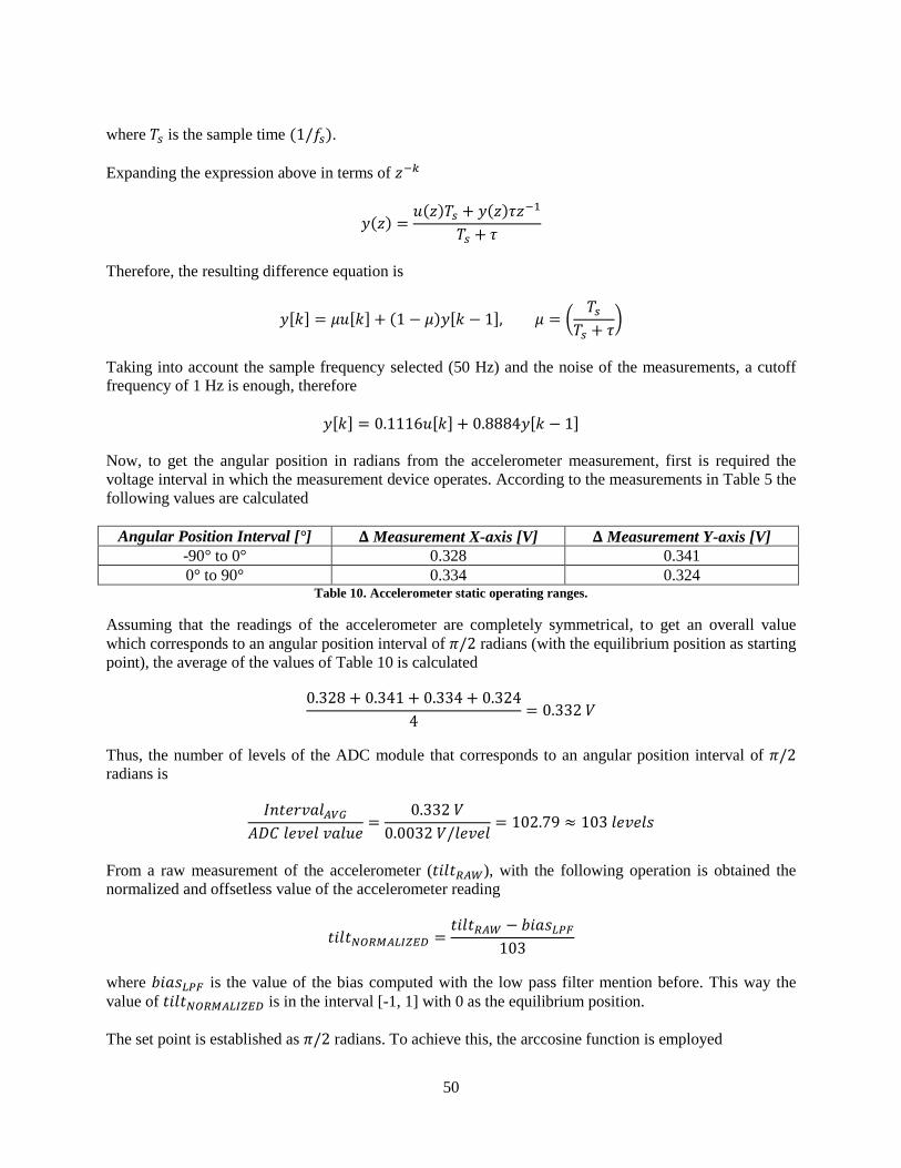
50
where is the sample time .
Expanding the expression above in terms of
Therefore, the resulting difference equation is
[ ] [ ] [ ] (
)
Taking into account the sample frequency selected (50 Hz) and the noise of the measurements, a cutoff
frequency of 1 Hz is enough, therefore
[ ] [ ] [ ]
Now, to get the angular position in radians from the accelerometer measurement, first is required the
voltage interval in which the measurement device operates. According to the measurements in Table 5 the
following values are calculated
Angular Position Interval [°] Measurement X-axis [V] Measurement Y-axis [V]
-90° to 0° 0.328 0.341
0° to 90° 0.334 0.324 Table 10. Accelerometer static operating ranges.
Assuming that the readings of the accelerometer are completely symmetrical, to get an overall value
which corresponds to an angular position interval of radians (with the equilibrium position as starting
point), the average of the values of Table 10 is calculated
Thus, the number of levels of the ADC module that corresponds to an angular position interval of
radians is
From a raw measurement of the accelerometer ( ), with the following operation is obtained the
normalized and offsetless value of the accelerometer reading
where is the value of the bias computed with the low pass filter mention before. This way the
value of is in the interval [-1, 1] with 0 as the equilibrium position.
The set point is established as radians. To achieve this, the arccosine function is employed
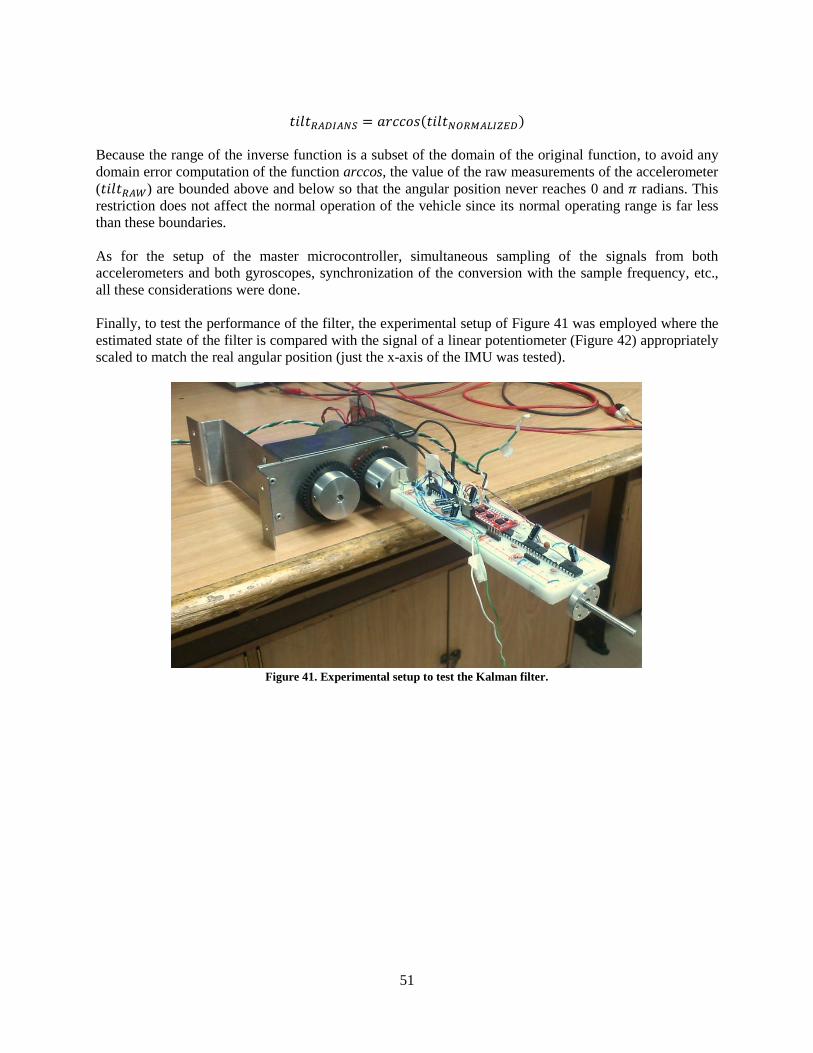
51
Because the range of the inverse function is a subset of the domain of the original function, to avoid any
domain error computation of the function arccos, the value of the raw measurements of the accelerometer
( ) are bounded above and below so that the angular position never reaches 0 and radians. This
restriction does not affect the normal operation of the vehicle since its normal operating range is far less
than these boundaries.
As for the setup of the master microcontroller, simultaneous sampling of the signals from both
accelerometers and both gyroscopes, synchronization of the conversion with the sample frequency, etc.,
all these considerations were done.
Finally, to test the performance of the filter, the experimental setup of Figure 41 was employed where the
estimated state of the filter is compared with the signal of a linear potentiometer (Figure 42) appropriately
scaled to match the real angular position (just the x-axis of the IMU was tested).
Figure 41. Experimental setup to test the Kalman filter.
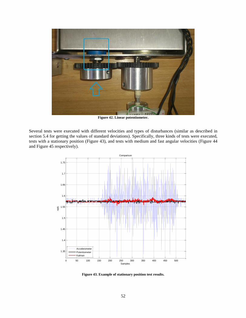
52
Figure 42. Linear potentiometer.
Several tests were executed with different velocities and types of disturbances (similar as described in
section 5.4 for getting the values of standard deviations). Specifically, three kinds of tests were executed,
tests with a stationary position (Figure 43), and tests with medium and fast angular velocities (Figure 44
and Figure 45 respectively).
Figure 43. Example of stationary position test results.
0 50 100 150 200 250 300 350 400 450 500
1.35
1.4
1.45
1.5
1.55
1.6
1.65
1.7
1.75
Comparison
Samples
rads
Accelerometer
Potentiometer
Kalman

53
Figure 44. Example of medium velocity test results.
Figure 45. Example of fast velocity test results.
0 50 100 150 200 250 300 350
0.6
0.8
1
1.2
1.4
1.6
1.8
2
2.2
2.4
2.6
Comparison
Samples
rads
Accelerometer
Potentiometer
Kalman
0 50 100 150 200 250 300 350
0.6
0.8
1
1.2
1.4
1.6
1.8
2
2.2
2.4
2.6
Comparison
Samples
rads
Accelerometer
Potentiometer
Kalman

54
Ten measurements for every test were executed. With the data recorded, the same comparisons made with
the simulations in subsection 5.4.2 are done. The mean squared error of the raw signal of the
accelerometer is compared with the mean squared error of the output of the filter . In
Table 11 are presented the average values of the results of every test.
Test [ ] [ ]
[ ]
Stationary 0.004433 0.000037 0.8330
Medium 0.033525 0.000754 2.2496
Fast 0.068188 0.001299 1.9053 Table 11. Average values of mean squared errors and ratio between these.
The overall average value of the comparison between the errors calculated is 1.6626 %. In average the
Kalman filter reduces the error in about 98.34 %, which proves the correspondence between the
simulations and the real measurements and filter computation.
6.4 Motor Control
The motor model must be validated to be able to design a controller using a mathematical model as real as
possible. The model parameters must be modified since the specifications given by the manufacturer are
not always reliable, and due to the full bridge driver used to control the motor which also has to be
included in the model.
On the other hand, to test the omnidirectionality of the vehicle a speed control must be implemented to
achieve an exact speed combination of the motors to drive the ball (wheel) with the desired direction
and/or desired rotation.
6.4.1 Model Validation
Before defining the controller of the motors, the theoretical model must be validated. A simple set of tests
were executed where different kind of inputs were applied to the theoretical model and the real plant in
open-loop to compare its outputs. Then, by modifying the values of the parameters of the model, the best
correspondence between the model and motor is attained.
To make the model as real as possible, the gearbox efficiency, which was disregarded before, is now
included and is treated as a gain. As done in subsection 5.2, a similar gearbox [34] with similar
parameters was chosen from the manufacturer Pittman® and, considering the ratio of the actual gearbox,
an efficiency of 75 percent was selected.
By setting the right values for the PWM module of the slave microcontrollers, the same inputs of the
simulations were put to the motor. Following the procedure mention before, the parameters that were
modified in order to achieve the best correspondence are presented in Table 12. It is noticed that the
magnitudes of the modified values are quite close to the magnitudes of the initial values selected for
initial simulations, therefore the analysis done so far regarding the actuators is still valid.
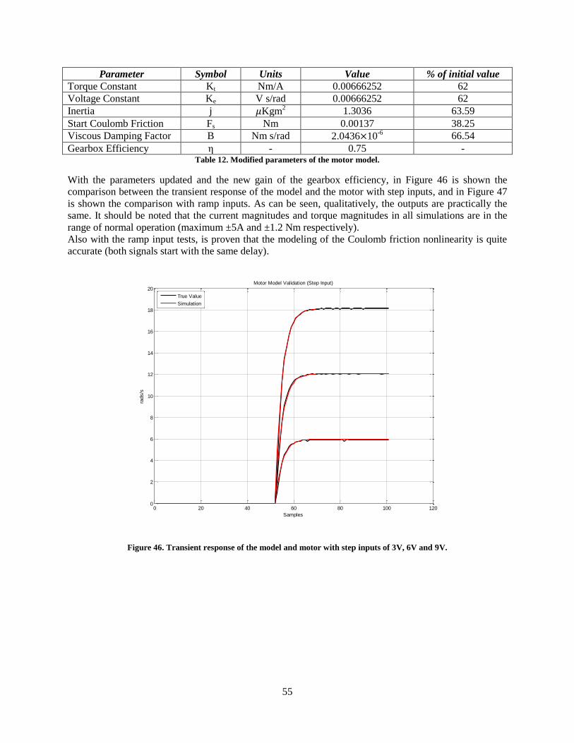
55
Parameter Symbol Units Value % of initial value
Torque Constant Kt Nm/A 0.00666252 62
Voltage Constant Ke V s/rad 0.00666252 62
Inertia j Kgm2 1.3036 63.59
Start Coulomb Friction Fs Nm 0.00137 38.25
Viscous Damping Factor B Nm s/rad 2.0436 10-6
66.54
Gearbox Efficiency η - 0.75 - Table 12. Modified parameters of the motor model.
With the parameters updated and the new gain of the gearbox efficiency, in Figure 46 is shown the
comparison between the transient response of the model and the motor with step inputs, and in Figure 47
is shown the comparison with ramp inputs. As can be seen, qualitatively, the outputs are practically the
same. It should be noted that the current magnitudes and torque magnitudes in all simulations are in the
range of normal operation (maximum ±5A and ±1.2 Nm respectively).
Also with the ramp input tests, is proven that the modeling of the Coulomb friction nonlinearity is quite
accurate (both signals start with the same delay).
Figure 46. Transient response of the model and motor with step inputs of 3V, 6V and 9V.
0 20 40 60 80 100 1200
2
4
6
8
10
12
14
16
18
20Motor Model Validation (Step Input)
Samples
rads/s
True Value
Simulation
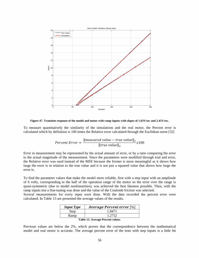
56
Figure 47. Transient response of the model and motor with ramp inputs with slopes of 1.63V/sec and 2.45V/sec.
To measure quantitatively the similarity of the simulations and the real motor, the Percent error is
calculated which by definition is 100 times the Relative error calculated through the Euclidean norm [32]
‖ ‖
‖ ‖
Error in measurement may be represented by the actual amount of error, or by a ratio comparing the error
to the actual magnitude of the measurement. Since the parameters were modified through trial and error,
the Relative error was used instead of the MSE because the former is more meaningful as it shows how
large the error is in relation to the true value and it is not just a squared value that shows how large the
error is.
To find the parameter values that make the model more reliable, first with a step input with an amplitude
of 6 volts, corresponding to the half of the operation range of the motor so the error over the range is
quasi-symmetric (due to model nonlinearities), was achieved the best likeness possible. Then, with the
ramp inputs test a fine-tuning was done and the value of the Coulomb friction was selected.
Several measurements for every input were done. With the data recorded the percent error were
calculated. In Table 13 are presented the average values of the results.
Input Type [ ] Step 1.8471
Ramp 1.2752 Table 13. Average Percent values.
Previous values are below the 2%, which proves that the correspondence between the mathematical
model and real motor is accurate. The average percent error of the tests with step inputs is a little bit
0 50 100 150 200 2500
2
4
6
8
10
12
14
16
18
20Motor Model Validation (Ramp Input)
Samples
rads/s
True Value
Simulation
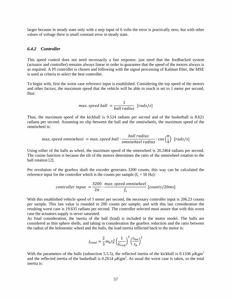
57
larger because in steady state only with a step input of 6 volts the error is practically zero, but with other
values of voltage there is small constant error in steady state.
6.4.2 Controller
This speed control does not need necessarily a fast response, just need that the feedbacked system
(actuator and controller) remains always linear in order to guarantee that the speed of the motors always is
as required. A PI controller is chosen and following with the signal processing of Kalman filter, the MSE
is used as criteria to select the best controller.
To begin with, first the worst case reference input is established. Considering the top speed of the motors
and other factors, the maximum speed that the vehicle will be able to reach is set to 1 meter per second,
thus:
[ ]
Thus, the maximum speed of the kickball is 9.524 radians per second and of the basketball is 8.621
radians per second. Assuming no slip between the ball and the omniwheels, the maximum speed of the
omniwheel is:
(
) [ ]
Using either of the balls as wheel, the maximum speed of the omniwheel is 20.2464 radians per second.
The cosine function is because the tilt of the motors determines the ratio of the omniwheel rotation to the
ball rotation [2].
Per revolution of the gearbox shaft the encoder generates 3200 counts, this way can be calculated the
reference input for the controller which is the counts per sample (fs = 50 Hz):
[ ]
With this established vehicle speed of 1 meter per second, the necessary controller input is 206.23 counts
per sample. This last value is rounded to 200 counts per sample, and with this last consideration the
resulting worst case is 19.635 radians per second. The controller selected must assure that with this worst
case the actuators supply is never saturated.
As final consideration, the inertia of the ball (load) is included in the motor model. The balls are
considered as thin sphere shells, and taking in consideration the gearbox reduction and the ratio between
the radius of the holonomic wheel and the balls, the load inertia reflected back to the motor is:
(
)
(
)
With the parameters of the balls (subsection 5.5.5), the reflected inertia of the kickball is 0.1336 Kgm2
and the reflected inertia of the basketball is 0.2614 Kgm2. As usual the worst case is taken, so the total
inertia is:
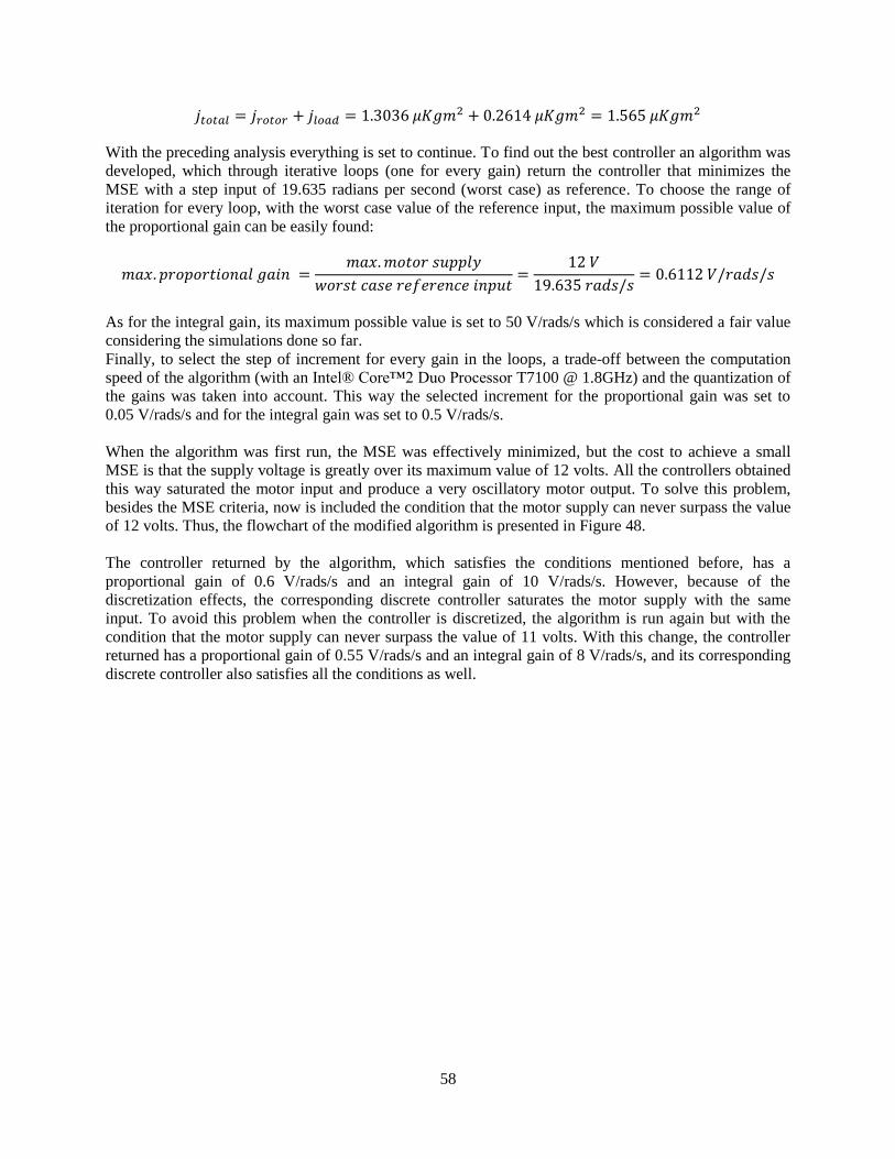
58
With the preceding analysis everything is set to continue. To find out the best controller an algorithm was
developed, which through iterative loops (one for every gain) return the controller that minimizes the
MSE with a step input of 19.635 radians per second (worst case) as reference. To choose the range of
iteration for every loop, with the worst case value of the reference input, the maximum possible value of
the proportional gain can be easily found:
As for the integral gain, its maximum possible value is set to 50 V/rads/s which is considered a fair value
considering the simulations done so far.
Finally, to select the step of increment for every gain in the loops, a trade-off between the computation
speed of the algorithm (with an Intel® Core™2 Duo Processor T7100 @ 1.8GHz) and the quantization of
the gains was taken into account. This way the selected increment for the proportional gain was set to
0.05 V/rads/s and for the integral gain was set to 0.5 V/rads/s.
When the algorithm was first run, the MSE was effectively minimized, but the cost to achieve a small
MSE is that the supply voltage is greatly over its maximum value of 12 volts. All the controllers obtained
this way saturated the motor input and produce a very oscillatory motor output. To solve this problem,
besides the MSE criteria, now is included the condition that the motor supply can never surpass the value
of 12 volts. Thus, the flowchart of the modified algorithm is presented in Figure 48.
The controller returned by the algorithm, which satisfies the conditions mentioned before, has a
proportional gain of 0.6 V/rads/s and an integral gain of 10 V/rads/s. However, because of the
discretization effects, the corresponding discrete controller saturates the motor supply with the same
input. To avoid this problem when the controller is discretized, the algorithm is run again but with the
condition that the motor supply can never surpass the value of 11 volts. With this change, the controller
returned has a proportional gain of 0.55 V/rads/s and an integral gain of 8 V/rads/s, and its corresponding
discrete controller also satisfies all the conditions as well.
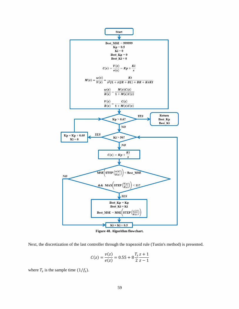
59
Figure 48. Algorithm flowchart.
Next, the discretization of the last controller through the trapezoid rule (Tustin's method) is presented.
where is the sample time .
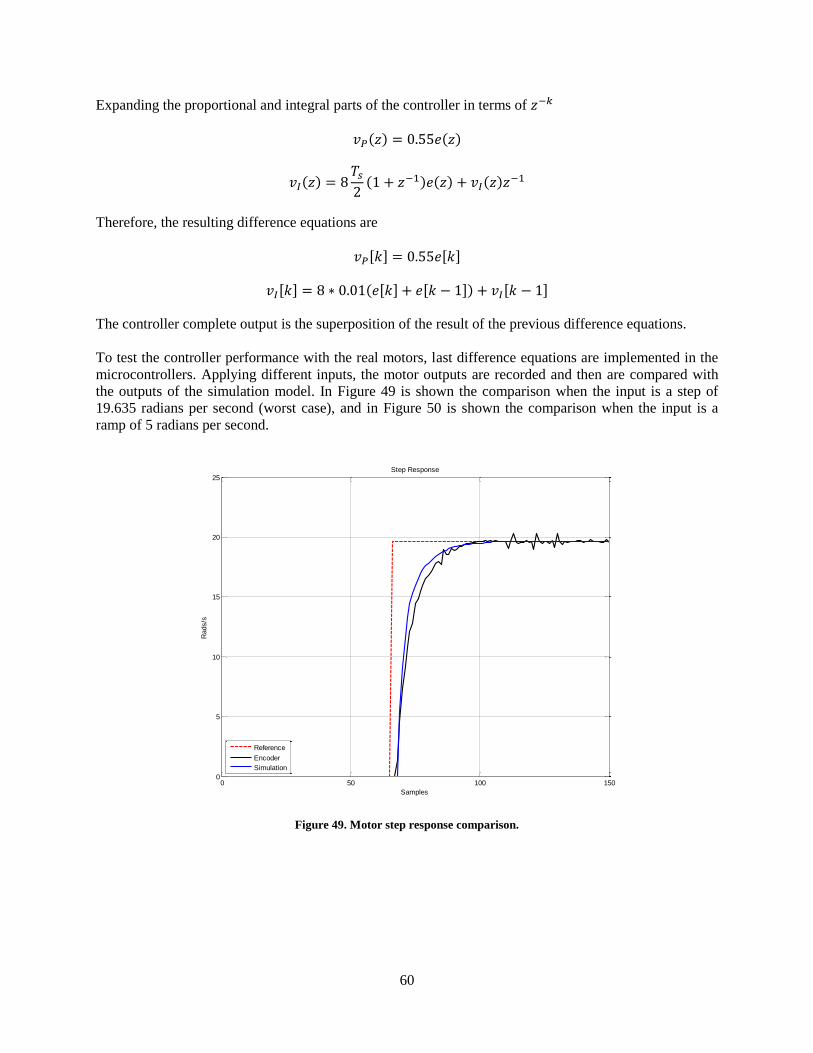
60
Expanding the proportional and integral parts of the controller in terms of
Therefore, the resulting difference equations are
[ ] [ ]
[ ] [ ] [ ] [ ]
The controller complete output is the superposition of the result of the previous difference equations.
To test the controller performance with the real motors, last difference equations are implemented in the
microcontrollers. Applying different inputs, the motor outputs are recorded and then are compared with
the outputs of the simulation model. In Figure 49 is shown the comparison when the input is a step of
19.635 radians per second (worst case), and in Figure 50 is shown the comparison when the input is a
ramp of 5 radians per second.
Figure 49. Motor step response comparison.
0 50 100 1500
5
10
15
20
25Step Response
Samples
Rads/s
Reference
Encoder
Simulation
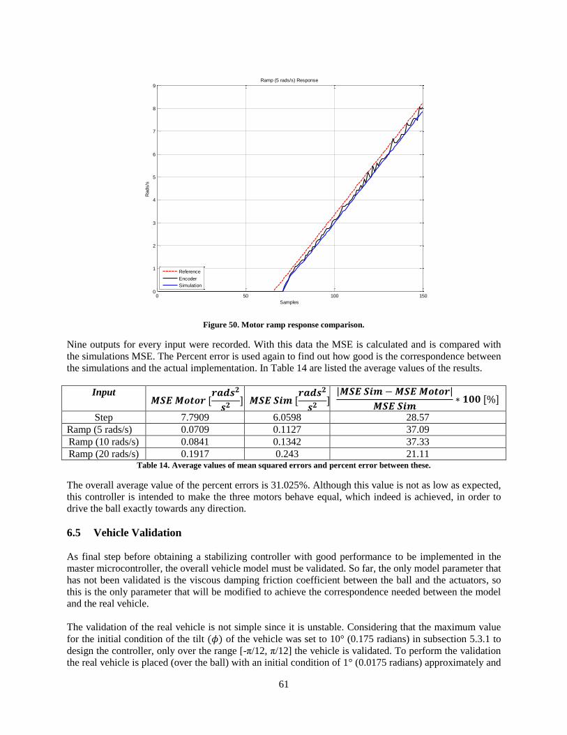
61
Figure 50. Motor ramp response comparison.
Nine outputs for every input were recorded. With this data the MSE is calculated and is compared with
the simulations MSE. The Percent error is used again to find out how good is the correspondence between
the simulations and the actual implementation. In Table 14 are listed the average values of the results.
Input [
] [
]
[ ]
Step 7.7909 6.0598 28.57
Ramp (5 rads/s) 0.0709 0.1127 37.09
Ramp (10 rads/s) 0.0841 0.1342 37.33
Ramp (20 rads/s) 0.1917 0.243 21.11 Table 14. Average values of mean squared errors and percent error between these.
The overall average value of the percent errors is 31.025%. Although this value is not as low as expected,
this controller is intended to make the three motors behave equal, which indeed is achieved, in order to
drive the ball exactly towards any direction.
6.5 Vehicle Validation
As final step before obtaining a stabilizing controller with good performance to be implemented in the
master microcontroller, the overall vehicle model must be validated. So far, the only model parameter that
has not been validated is the viscous damping friction coefficient between the ball and the actuators, so
this is the only parameter that will be modified to achieve the correspondence needed between the model
and the real vehicle.
The validation of the real vehicle is not simple since it is unstable. Considering that the maximum value
for the initial condition of the tilt of the vehicle was set to 10° (0.175 radians) in subsection 5.3.1 to
design the controller, only over the range [-π/12, π/12] the vehicle is validated. To perform the validation
the real vehicle is placed (over the ball) with an initial condition of 1° (0.0175 radians) approximately and
0 50 100 1500
1
2
3
4
5
6
7
8
9Ramp (5 rads/s) Response
Samples
Rads/s
Reference
Encoder
Simulation
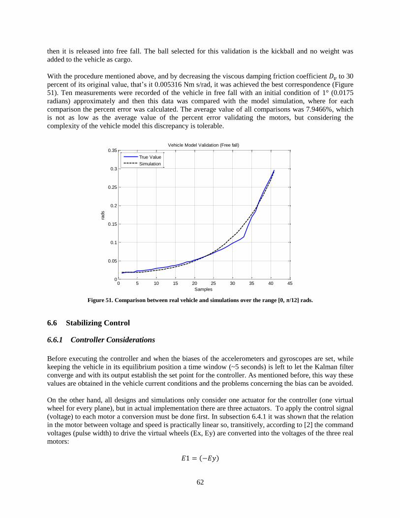
62
then it is released into free fall. The ball selected for this validation is the kickball and no weight was
added to the vehicle as cargo.
With the procedure mentioned above, and by decreasing the viscous damping friction coefficient to 30
percent of its original value, that’s it 0.005316 Nm s/rad, it was achieved the best correspondence (Figure
51). Ten measurements were recorded of the vehicle in free fall with an initial condition of 1° (0.0175
radians) approximately and then this data was compared with the model simulation, where for each
comparison the percent error was calculated. The average value of all comparisons was 7.9466%, which
is not as low as the average value of the percent error validating the motors, but considering the
complexity of the vehicle model this discrepancy is tolerable.
Figure 51. Comparison between real vehicle and simulations over the range [0, π/12] rads.
6.6 Stabilizing Control
6.6.1 Controller Considerations
Before executing the controller and when the biases of the accelerometers and gyroscopes are set, while
keeping the vehicle in its equilibrium position a time window (~5 seconds) is left to let the Kalman filter
converge and with its output establish the set point for the controller. As mentioned before, this way these
values are obtained in the vehicle current conditions and the problems concerning the bias can be avoided.
On the other hand, all designs and simulations only consider one actuator for the controller (one virtual
wheel for every plane), but in actual implementation there are three actuators. To apply the control signal
(voltage) to each motor a conversion must be done first. In subsection 6.4.1 it was shown that the relation
in the motor between voltage and speed is practically linear so, transitively, according to [2] the command
voltages (pulse width) to drive the virtual wheels (Ex, Ey) are converted into the voltages of the three real
motors:
0 5 10 15 20 25 30 35 40 450
0.05
0.1
0.15
0.2
0.25
0.3
0.35Vehicle Model Validation (Free fall)
Samples
rads
True Value
Simulation
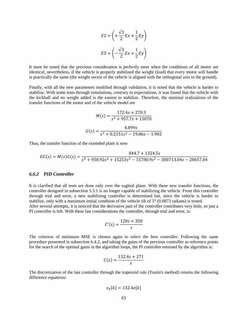
63
(
)
(
)
It must be noted that the previous consideration is perfectly meet when the conditions of all motor are
identical, nevertheless, if the vehicle is properly stabilized the weight (load) that every motor will handle
is practically the same (the weight vector of the vehicle is aligned with the orthogonal axis to the ground).
Finally, with all the new parameters modified through validation, it is noted that the vehicle is harder to
stabilize. With some tests through simulations, contrary to expectations, it was found that the vehicle with
the kickball and no weight added is the easiest to stabilize. Therefore, the minimal realizations of the
transfer functions of the motor and of the vehicle model are
Thus, the transfer function of the extended plant is now
6.6.2 PID Controller
It is clarified that all tests are done only over the sagittal plane. With these new transfer functions, the
controller designed in subsection 5.3.1 is no longer capable of stabilizing the vehicle. From this controller
through trial and error, a new stabilizing controller is determined but, since the vehicle is harder to
stabilize, only with a maximum initial condition of the vehicle tilt of 5° (0.0873 radians) is tested.
After several attempts, it is noticed that the derivative part of the controller contributes very little, so just a
PI controller is left. With these last considerations the controller, through trial and error, is:
The criterion of minimum MSE is chosen again to select the best controller. Following the same
procedure presented in subsection 6.4.2, and taking the gains of the previous controller as reference points
for the search of the optimal gains in the algorithm loops, the PI controller returned by the algorithm is:
The discretization of the last controller through the trapezoid rule (Tustin's method) returns the following
difference equations:
[ ] [ ]
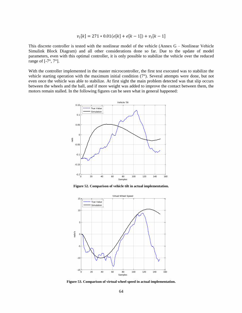
64
[ ] [ ] [ ] [ ]
This discrete controller is tested with the nonlinear model of the vehicle (Annex G – Nonlinear Vehicle
Simulink Block Diagram) and all other considerations done so far. Due to the update of model
parameters, even with this optimal controller, it is only possible to stabilize the vehicle over the reduced
range of [-7°, 7°].
With the controller implemented in the master microcontroller, the first test executed was to stabilize the
vehicle starting operation with the maximum initial condition (7°). Several attempts were done, but not
even once the vehicle was able to stabilize. At first sight the main problem detected was that slip occurs
between the wheels and the ball, and if more weight was added to improve the contact between them, the
motors remain stalled. In the following figures can be seen what in general happened:
Figure 52. Comparison of vehicle tilt in actual implementation.
Figure 53. Comparison of virtual wheel speed in actual implementation.
0 20 40 60 80 100 120 140 160-0.2
-0.15
-0.1
-0.05
0
0.05
0.1
0.15Vehicle Tilt
Samples
rads
True Value
Simulation
0 20 40 60 80 100 120 140 160-15
-10
-5
0
5
10
15Virtual Wheel Speed
Samples
rads/s
True Value
Simulation
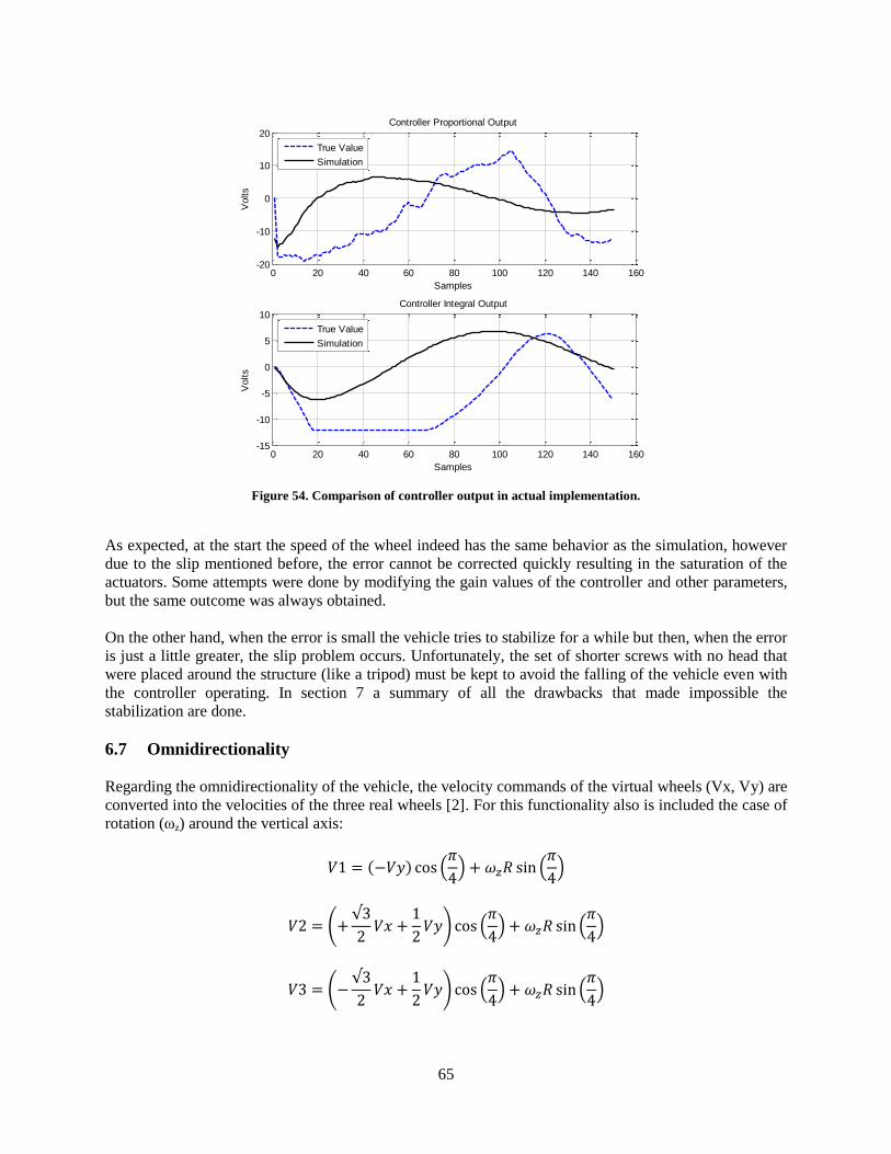
65
Figure 54. Comparison of controller output in actual implementation.
As expected, at the start the speed of the wheel indeed has the same behavior as the simulation, however
due to the slip mentioned before, the error cannot be corrected quickly resulting in the saturation of the
actuators. Some attempts were done by modifying the gain values of the controller and other parameters,
but the same outcome was always obtained.
On the other hand, when the error is small the vehicle tries to stabilize for a while but then, when the error
is just a little greater, the slip problem occurs. Unfortunately, the set of shorter screws with no head that
were placed around the structure (like a tripod) must be kept to avoid the falling of the vehicle even with
the controller operating. In section 7 a summary of all the drawbacks that made impossible the
stabilization are done.
6.7 Omnidirectionality
Regarding the omnidirectionality of the vehicle, the velocity commands of the virtual wheels (Vx, Vy) are
converted into the velocities of the three real wheels [2]. For this functionality also is included the case of
rotation (ωz) around the vertical axis:
(
) (
)
(
) (
) (
)
(
) (
) (
)
0 20 40 60 80 100 120 140 160-20
-10
0
10
20Controller Proportional Output
Samples
Volts
True Value
Simulation
0 20 40 60 80 100 120 140 160-15
-10
-5
0
5
10Controller Integral Output
Samples
Volts
True Value
Simulation
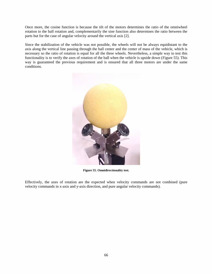
66
Once more, the cosine function is because the tilt of the motors determines the ratio of the omniwheel
rotation to the ball rotation and, complementarily the sine function also determines the ratio between the
parts but for the case of angular velocity around the vertical axis [2].
Since the stabilization of the vehicle was not possible, the wheels will not be always equidistant to the
axis along the vertical line passing through the ball center and the center of mass of the vehicle, which is
necessary so the ratio of rotation is equal for all the three wheels. Nevertheless, a simple way to test this
functionality is to verify the axes of rotation of the ball when the vehicle is upside down (Figure 55). This
way is guaranteed the previous requirement and is ensured that all three motors are under the same
conditions.
Figure 55. Omnidirectionality test.
Effectively, the axes of rotation are the expected when velocity commands are not combined (pure
velocity commands in x-axis and y-axis direction, and pure angular velocity commands).
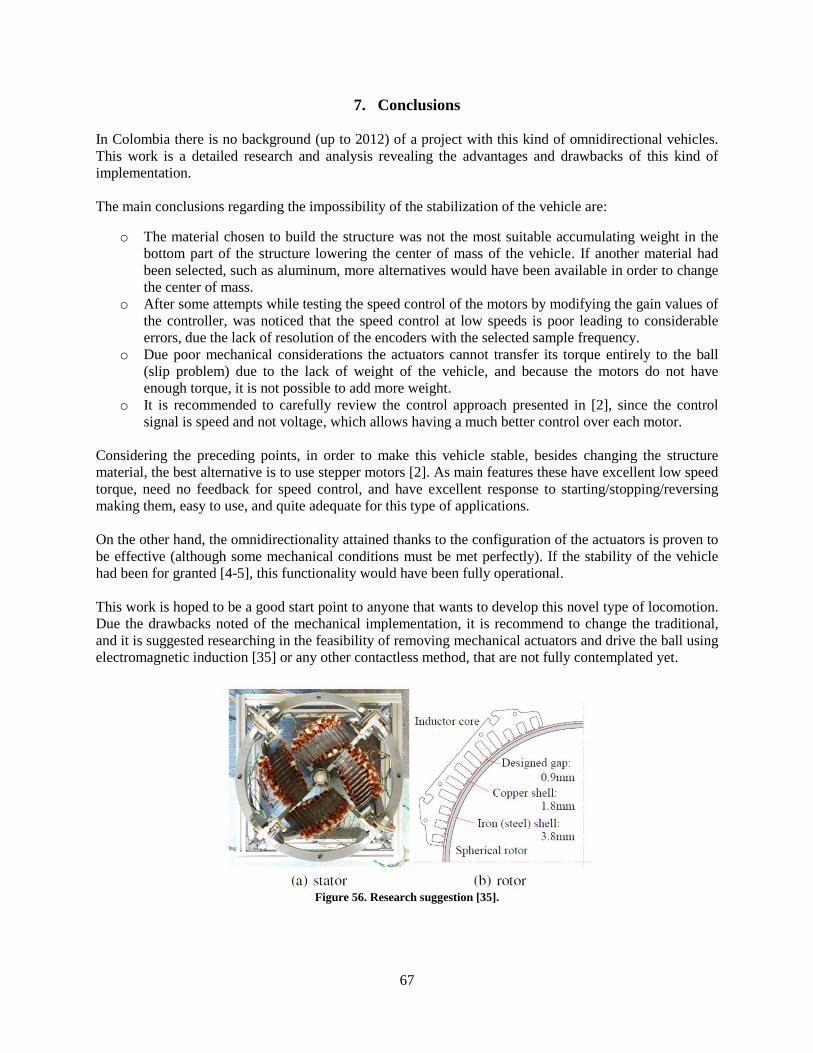
67
7. Conclusions
In Colombia there is no background (up to 2012) of a project with this kind of omnidirectional vehicles.
This work is a detailed research and analysis revealing the advantages and drawbacks of this kind of
implementation.
The main conclusions regarding the impossibility of the stabilization of the vehicle are:
o The material chosen to build the structure was not the most suitable accumulating weight in the
bottom part of the structure lowering the center of mass of the vehicle. If another material had
been selected, such as aluminum, more alternatives would have been available in order to change
the center of mass.
o After some attempts while testing the speed control of the motors by modifying the gain values of
the controller, was noticed that the speed control at low speeds is poor leading to considerable
errors, due the lack of resolution of the encoders with the selected sample frequency.
o Due poor mechanical considerations the actuators cannot transfer its torque entirely to the ball
(slip problem) due to the lack of weight of the vehicle, and because the motors do not have
enough torque, it is not possible to add more weight.
o It is recommended to carefully review the control approach presented in [2], since the control
signal is speed and not voltage, which allows having a much better control over each motor.
Considering the preceding points, in order to make this vehicle stable, besides changing the structure
material, the best alternative is to use stepper motors [2]. As main features these have excellent low speed
torque, need no feedback for speed control, and have excellent response to starting/stopping/reversing
making them, easy to use, and quite adequate for this type of applications.
On the other hand, the omnidirectionality attained thanks to the configuration of the actuators is proven to
be effective (although some mechanical conditions must be met perfectly). If the stability of the vehicle
had been for granted [4-5], this functionality would have been fully operational.
This work is hoped to be a good start point to anyone that wants to develop this novel type of locomotion.
Due the drawbacks noted of the mechanical implementation, it is recommend to change the traditional,
and it is suggested researching in the feasibility of removing mechanical actuators and drive the ball using
electromagnetic induction [35] or any other contactless method, that are not fully contemplated yet.
Figure 56. Research suggestion [35].
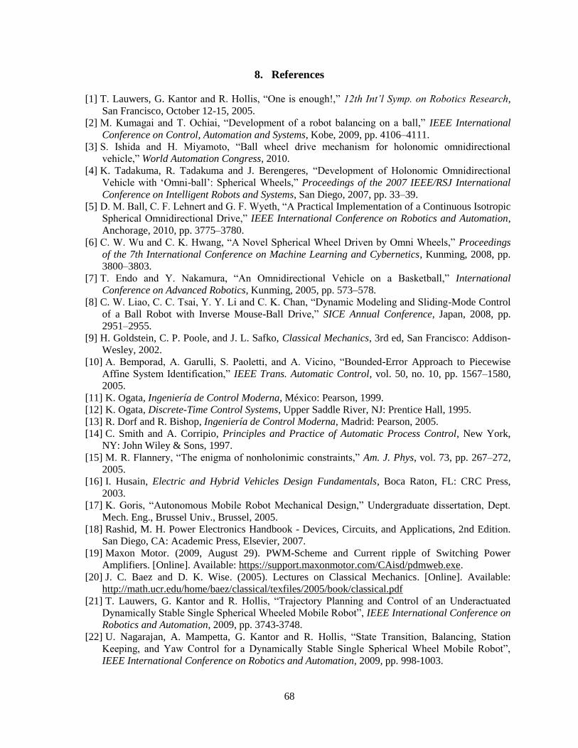
68
8. References
[1] T. Lauwers, G. Kantor and R. Hollis, “One is enough!,” 12th Int’l Symp. on Robotics Research,
San Francisco, October 12-15, 2005.
[2] M. Kumagai and T. Ochiai, “Development of a robot balancing on a ball,” IEEE International
Conference on Control, Automation and Systems, Kobe, 2009, pp. 4106–4111.
[3] S. Ishida and H. Miyamoto, “Ball wheel drive mechanism for holonomic omnidirectional
vehicle,” World Automation Congress, 2010.
[4] K. Tadakuma, R. Tadakuma and J. Berengeres, “Development of Holonomic Omnidirectional
Vehicle with ‘Omni-ball’: Spherical Wheels,” Proceedings of the 2007 IEEE/RSJ International
Conference on Intelligent Robots and Systems, San Diego, 2007, pp. 33–39.
[5] D. M. Ball, C. F. Lehnert and G. F. Wyeth, “A Practical Implementation of a Continuous Isotropic
Spherical Omnidirectional Drive,” IEEE International Conference on Robotics and Automation,
Anchorage, 2010, pp. 3775–3780.
[6] C. W. Wu and C. K. Hwang, “A Novel Spherical Wheel Driven by Omni Wheels,” Proceedings
of the 7th International Conference on Machine Learning and Cybernetics, Kunming, 2008, pp.
3800–3803.
[7] T. Endo and Y. Nakamura, “An Omnidirectional Vehicle on a Basketball,” International
Conference on Advanced Robotics, Kunming, 2005, pp. 573–578.
[8] C. W. Liao, C. C. Tsai, Y. Y. Li and C. K. Chan, “Dynamic Modeling and Sliding-Mode Control
of a Ball Robot with Inverse Mouse-Ball Drive,” SICE Annual Conference, Japan, 2008, pp.
2951–2955.
[9] H. Goldstein, C. P. Poole, and J. L. Safko, Classical Mechanics, 3rd ed, San Francisco: Addison-
Wesley, 2002.
[10] A. Bemporad, A. Garulli, S. Paoletti, and A. Vicino, “Bounded-Error Approach to Piecewise
Affine System Identification,” IEEE Trans. Automatic Control, vol. 50, no. 10, pp. 1567–1580,
2005.
[11] K. Ogata, Ingeniería de Control Moderna, México: Pearson, 1999.
[12] K. Ogata, Discrete-Time Control Systems, Upper Saddle River, NJ: Prentice Hall, 1995.
[13] R. Dorf and R. Bishop, Ingeniería de Control Moderna, Madrid: Pearson, 2005.
[14] C. Smith and A. Corripio, Principles and Practice of Automatic Process Control, New York,
NY: John Wiley & Sons, 1997.
[15] M. R. Flannery, “The enigma of nonholonimic constraints,” Am. J. Phys, vol. 73, pp. 267–272,
2005.
[16] I. Husain, Electric and Hybrid Vehicles Design Fundamentals, Boca Raton, FL: CRC Press,
2003.
[17] K. Goris, “Autonomous Mobile Robot Mechanical Design,” Undergraduate dissertation, Dept.
Mech. Eng., Brussel Univ., Brussel, 2005.
[18] Rashid, M. H. Power Electronics Handbook - Devices, Circuits, and Applications, 2nd Edition.
San Diego, CA: Academic Press, Elsevier, 2007.
[19] Maxon Motor. (2009, August 29). PWM-Scheme and Current ripple of Switching Power
Amplifiers. [Online]. Available: https://support.maxonmotor.com/CAisd/pdmweb.exe.
[20] J. C. Baez and D. K. Wise. (2005). Lectures on Classical Mechanics. [Online]. Available:
http://math.ucr.edu/home/baez/classical/texfiles/2005/book/classical.pdf
[21] T. Lauwers, G. Kantor and R. Hollis, “Trajectory Planning and Control of an Underactuated
Dynamically Stable Single Spherical Wheeled Mobile Robot”, IEEE International Conference on
Robotics and Automation, 2009, pp. 3743-3748.
[22] U. Nagarajan, A. Mampetta, G. Kantor and R. Hollis, “State Transition, Balancing, Station
Keeping, and Yaw Control for a Dynamically Stable Single Spherical Wheel Mobile Robot”,
IEEE International Conference on Robotics and Automation, 2009, pp. 998-1003.
69
[23] G. Durrant-Whyte, “Multi Sensor Data Fusion”, Australian Centre for Field Robotics, Sydney
Univ., Sydney, 2001.
[24] G. Welch and G. Bishop. (2001). An Introduction to the Kalman Filter [Online], Available:
http://www.cs.unc.edu/~tracker/media/pdf/SIGGRAPH2001_CoursePack_08.pdf
[25] B. Borchers and R. Aster. (2011). Notes on Kalman Filtering [Online], Available:
http://www.ees.nmt.edu/outside/courses/GEOP505/Docs/kalman.pdf
[26] M. Isabel Ribeiro, "Kalman and Extended Kalman Filters: Concept, Derivation and Properties",
Instituto de Sistemas e Robótica, Instituto Superio Técnico, February 2004.
[27] Microchip Technology Inc., dsPIC33FJ06GS101/X02 and dsPIC33FJ16GSX02/X04 Data Sheet,
Revision D, March 2009.
[28] Microchip Technology Inc., dsPIC33FJ32MC302/304, dsPIC33FJ64MCX02/X04 and
dsPIC33FJ128MCX02/X04 Data Sheet, Revision E, January 2011.
[29] Analog Devices Inc., Application Note 1057 - Using an Accelerometer for Inclination Sensing,
Revision 0, 2010.
[30] IPC - Association Connecting Electronics Industries, IPC-2221 Generic Standard on Printed
Board Design, Illinois, February 1998.
[31] IPC - Association Connecting Electronics Industries, IPC-2222 Sectional Design Standard for
Rigid Organic Printed Boards, Illinois, February 1998.
[32] G. Golub and C. F. Van Loan, Matrix Computations, 3rd ed, Baltimore: The Johns Hopkins
University Press, 1996.
[33] AMETEK Precision Motion Control - PITTMAN, Brush Commutated DC Servo Motors - 8541
Series, Revision 0, 2013.
[34] AMETEK Precision Motion Control - PITTMAN, Gearboxes - G30A Planetary Gearbox,
Revision 0, 2013.
[35] M. Kumagai, R.L. Hollis, “Development and Control of a Three DOF Spherical Induction
Motor”, ICRA 2013, pp. 1520–1525, 2013.
70
9. Annexes
9.1 Annex A – Lagrangian Mechanics
9.1.1 Generalized Coordinates Working with systems with multiple bodies, the generalized coordinates are a set of coordinates used to
describe the configuration of a system relative to some reference setup. A restriction for a set of
coordinates, to serve as generalized coordinates, is that they should uniquely define any possible
configuration of the system relative to the reference setup.
For Lagrangian mechanics is quite useful using generalized coordinates, these are the { }. The are
generalized positions, and the are generalized velocities. The set of independent generalized
coordinates describe the motion of the system completely and its number is equal to the degrees of
freedom of the system [20]. If a system requires n generalized coordinates, these can be considered as the
coordinates of an n-dimensional coordinate system in an n-dimensional space. As time elapses, the system
point, in the n-dimensional space, moves and describes a curve in the space, and so this curve represents
the motion of the system point. Note that the space mention before has no necessary connection with the
three-dimensional space, just as the generalized coordinates are not necessarily position coordinates. The
path of motion described in this n-dimensional space has no resemblance to the path in space of any
actual particle; each point on the path represents the entire system configuration at some given instant of
time [9].
9.1.2 Hamilton´s Principle As mention before, Newton's laws are relationships among vectors, which is why they get so messy when
we change coordinate systems. The Lagrangian formulation, on the other hand, just uses scalars, and so
coordinate transformations tend to be much easier. Given a Lagrangian L (it can be defined more than
one), which is a function of the location in space and the velocity, we define the “action”
∫
Regarding the behavior of the system, one can imagine the system taking many paths (on the n-
dimensional space), whether they obey Newton's Laws or not, nevertheless Hamilton's principle states
that the true evolution of a system, described by n generalized coordinates from
time t1 to time t2, is such that the line integral (called action), has a stationary value. That is, out of all
possible paths by which system point could travel from a fixed position at time t1 to another fixed
position at time t2, it will actually travel along that path for which the value of the integral is minimized
(path of least action). Basically, the notion of a stationary value for a line integral corresponds, in ordinary
function theory, to the vanishing of the first derivate [9]. The Hamilton’s principle can be summarize by
saying that the motion of the system is such that the variation of the line integral S for fixed t1 and t2 is
zero
∫
A straightforward way to understand the meaning of this principle is as stated next:
“…the Lagrangian measures something we could vaguely refer to as the ‘activity’ or ‘liveliness’ of a
system: the higher the kinetic energy the more lively the system, the higher the potential energy the less
71
lively. So, we're being told that nature likes to minimize the total of ‘liveliness’ over time: that is, the total
action. In other words, nature is as lazy as possible!” [20].
A great advantage of this approach is that the path of least action is the same, no matter what coordinates
you use, it's just the integral over time of a scalar (its value will not change, no matter how you choose to
measure distances in space). So, to find the equations of motion in an arbitrary coordinate system , it is
only necessary to express the kinetic and potential energy of the system in terms of the selected
coordinates [20].
9.1.3 Euler-Lagrange equations of motion for conservative systems If no energy is dissipated in a system, it is called a conservative system. A conservative mechanical
system is one in which energy appears only as kinetic energy and potential energy.
Let represent the true evolution of the system between two fixed states and at two
specified times t1 and t2. Let us assume that is an arbitrary function that is continuous in t1 < t < t2,
has a continuous derivate in t1 < t < t2 and vanishes at t = t1 and t = t2, or = = 0.
According to Hamilton´s principle by nullifying the first derivate of the action S, the true behavior of a
system can be obtained, so:
∫
applying the chain rule to derivate, it is obtained
∫ (
)
rearranging terms
∫
∫
∫
∫
by integrating the second term by parts, the result is
∫
∫
(
)
∫ (
(
))
The boundary terms each have a factor of at the initial and final point, which vanish because
Hamilton´s principle states that and are fixed, so is equal to zero if and only if the
integrand of the remaining term must zero as well
72
(
)
From the expression above, a set of differential equations for can be derived which represent the true
behavior of a system. These equations are called the ‘Euler-Lagrange Equations’.
9.1.4 Euler-Lagrange equations of motion for non-conservative systems If there are non-conservative forces (damped systems), the scheme that has been outlined so far does not
fit neatly. When not all the forces acting on a system are derivable from a potential, then Lagrange’s
equations can be written in the form [9]
(
)
where L contains the potential of the conservative forces, and Qj represents the forces not arising from a
potential. Such a situation often occurs when frictional forces are present. It frequently happens that the
frictional force is proportional to the velocity of the particle, so that its x-component has the form [9]
Frictional forces of this type may be derived in terms of a function F, known as Rayleigh’s dissipation
function which is defined as
∑
where the summation is over the particles of the system. From this definition it is clear that
or, symbolically
Since the velocities can be expressed as a function of the generalized velocities , by using Rayleigh’s
dissipation function, Lagrange’s equations for non-conservative systems become
(
)
73
9.2 Annex B – Discrete Kalman Filter Gain Derivation
A discrete time linear system is simply a process that can be described by the following two equations
[ ] [ ] [ ] [ ]
[ ] [ ] [ ]
where the variable v is called the process noise, and w is called the measurement or observation noise.
A basic assumption in the derivation of the Kalman filter is that the random sequences [ ] and [ ] describing process and observation noise are all Gaussian and zero-mean
{ [ ]} { [ ]}
with known covariance
{ [ ] [ ]} [ ] { [ ] [ ]} [ ]
It is also generally assumed that the process and observation noises are also uncorrelated
{ [ ] [ ]}
These assumptions are not absolutely necessary. It is relatively simple, but algebraically complex, to
include a term for the correlation between process and observation errors. Also, if the sequences are not
Gaussian, but are symmetric with finite moments, then the Kalman filter will be able to produce good
estimates. However, if the sequences have an ‘irregular’ distribution, results produced by the Kalman
filter will not be accurate and perhaps a more sophisticated filter will be more suitable [23].
Defining the error as the difference between the real state and the estimation
[ ] [ ] [ ]
The objective is to minimize the mean squared error
∑ [ ] [ ]
{ [ ] [ ]} [ ]
where is known as error covariance matrix.
Basically the filter consists in determine the value of the estimated states [ ] from the contaminated
measurements [ ] in order that the matrix [ ] is minimized (actually the trace of [ ] is which
contains the covariance of the errors with themselves, that is its variance , which are the values that
really are needed to be minimized [25].
The algorithm has two main steps that are computed iteratively. The first one is to predict the states [ ] and then the correction or update of the estimated states [ ].
The prediction of the states is computed as follows
74
[ ] [ ] [ ]
where [ ] are the last estimated states.
Now the error covariance matrix (mean squared error) is predicted (which is needed in the further
analysis), through the predicted error [ ]
[ ] [ ] [ ]
[ ] [ ] [ ] [ ] [ ] [ ]
[ ] { [ ] [ ]} {[ [ ] [ ] [ ]][ [ ] [ ] [ ]] }
[ ] {[ [ ] [ ] ][ [ ] [ ] ] } { [ ] [ ]}
[ ] [ ] [ ]
where [ ] is defined as the process noise covariance matrix, and [ ] is the last estimated error
covariance matrix calculated.
The estimation is going to be computed through the last predicted state [ ] and a correction that is
function of the error between the last measurement taken [ ] and the predicted output [ ]
[ ] [ ] [ ] [ ] [ ]
where [ ] is the gain (Kalman gain) which weights the correction that minimizes the error.
The last measurement taken has the value
[ ] [ ] [ ]
With the preceding analysis, the correction or update of the estimated states [ ] is done by rewriting
the error between the real state and the estimation
[ ] [ ] [ ]
[ ] [ ] ( [ ] [ ] [ ] [ ] )
[ ] [ ] ( [ ] [ ] [ ] [ ] [ ] )
[ ] [ ] [ ] [ ] [ ] [ ]
The estimated error covariance matrix (mean squared error) is computed through the rewritten error
[ ]
75
[ ] { [ ] [ ]}
{[ [ ] [ ] [ ]
[ ] [ ]][ [ ] [ ] [ ] [ ] [ ]] }
[ ] {[ [ ] [ ] [ ] ][ [ ] [ ] [ ] ] } { [ ] [ ] [ ] [ ]}
[ ] [ ] [ [ ] [ ] [ ] [ ] ] [ ] [ ] [ ] [ ]
where [ ] is defined as the measurement noise covariance matrix.
The predicted error covariance matrix [ ] also can be rewritten as follows
[ ] {[ [ ] [ ] [ ]][ [ ] [ ] [ ]] }
[ ] { [ ] [ ] [ ] [ ] }
So:
[ ] [ ] [ ] [ ] [ ] [ ] [ ]
For simplicity let
[ ] [ ] [ ] [ ]
Expanding [ ]
The estimated error covariance matrix is differentiated with respect to the gain and the result is
equaled to zero to find which value of minimizes it. As mention before, the trace of is which contains
the values that really are needed to be minimized, therefore, taking advantage of the properties of traces,
transposes and symmetric matrices, the optimal value of the gain is
( ) ( ) ( ) ( )
( ) ( ) ( )
Putting aside the traces
( )
( )
76
Finally, in order the filter can be executed, the value of [ ] is needed to compute the next
prediction. To get the minimal expression of [ ], first the value of the measurement noise
covariance matrix is obtained from the expression of the optimal value of
Now it is replaced in the expansion of [ ]
( )
( )
In practice, the process noise covariance and measurement noise covariance matrices might change
with each time step or measurement, however it can be assumed that they are constant, in order the
implementation of the filter is practical and efficient [24].
To perform the filter, everything is reduced to compute the following operations
[ ] [ ] [ ]
[ ] [ ]
[ ] [ ] ( [ ] )
[ ] [ ] [ ] [ ] [ ]
[ ] [ ] [ ]
The Kalman filter to work correctly it is necessary to assume certain initial values to execute the first
prediction. If information about [ ] and [ ] is known a priori, the best that can be said is that the
system initial state coincides with the mean value of the random vector [26]
[ ] [ ]
[ ] [ ]
On the contrary, when information about [ ] and [ ] is not known, the filter initialization cannot
accurately reflect the system initial conditions, then a good alternative is [26]

77
[ ] [ ]
where is a scalar.
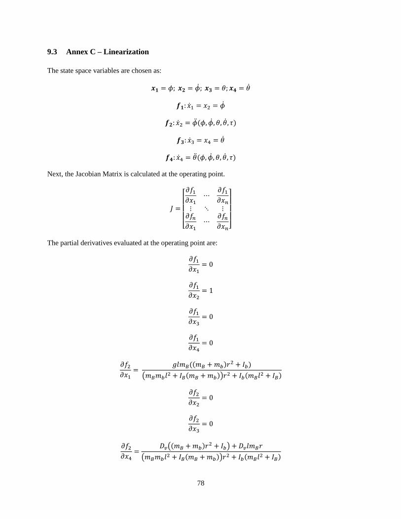
78
9.3 Annex C – Linearization
The state space variables are chosen as:
Next, the Jacobian Matrix is calculated at the operating point.
[
]
The partial derivatives evaluated at the operating point are:
( )
(
)
( )
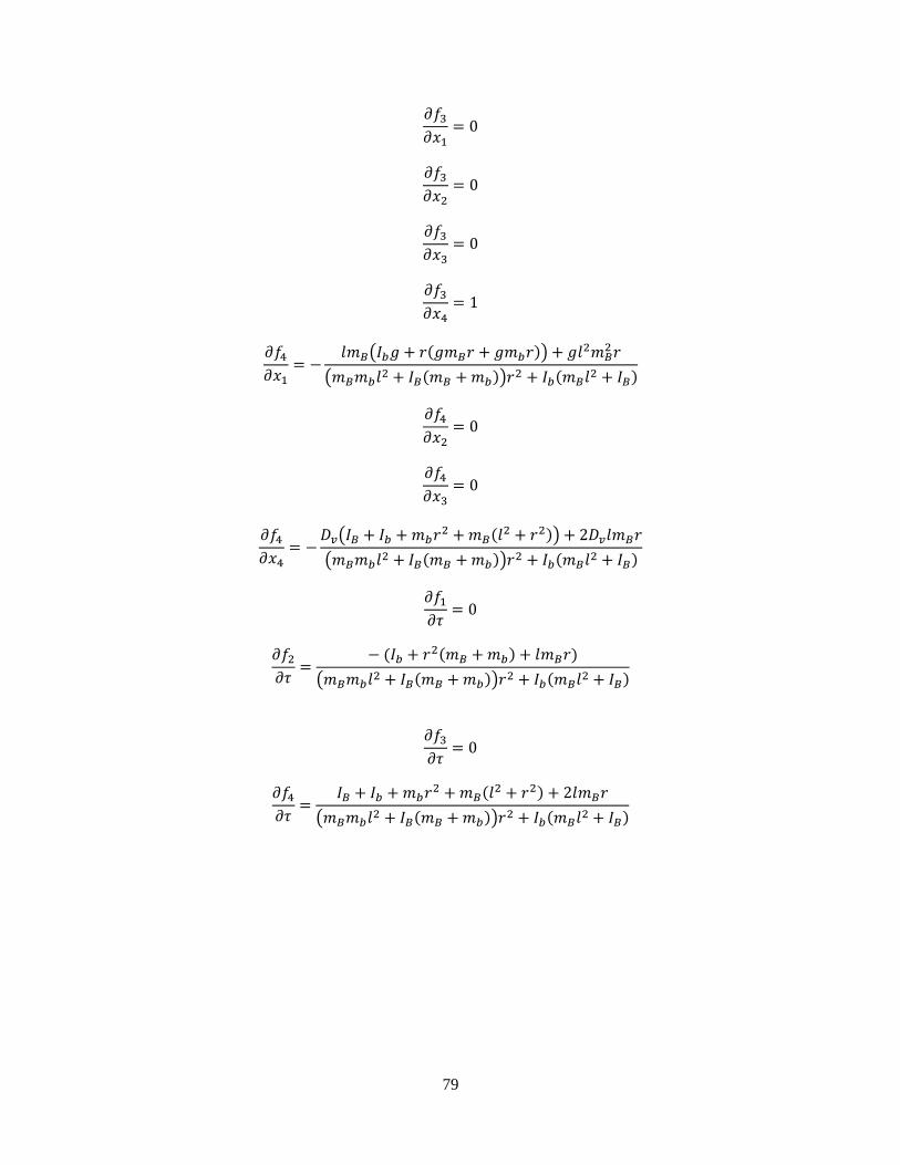
79
( )
( )
(
)
( )
( )
( )
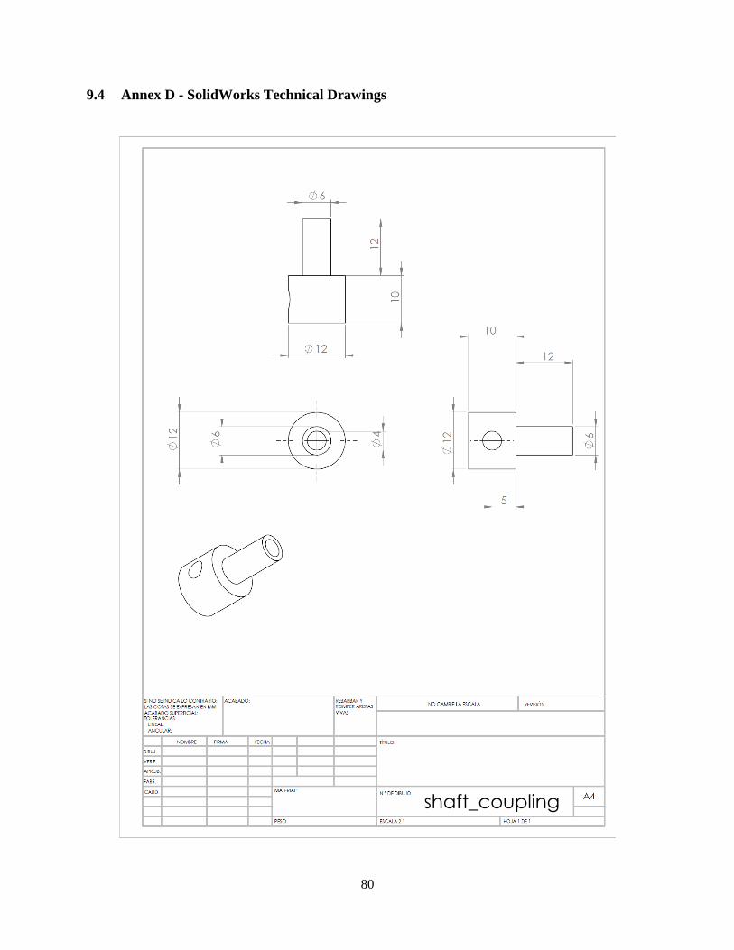
80
9.4 Annex D - SolidWorks Technical Drawings
shaft_coupling
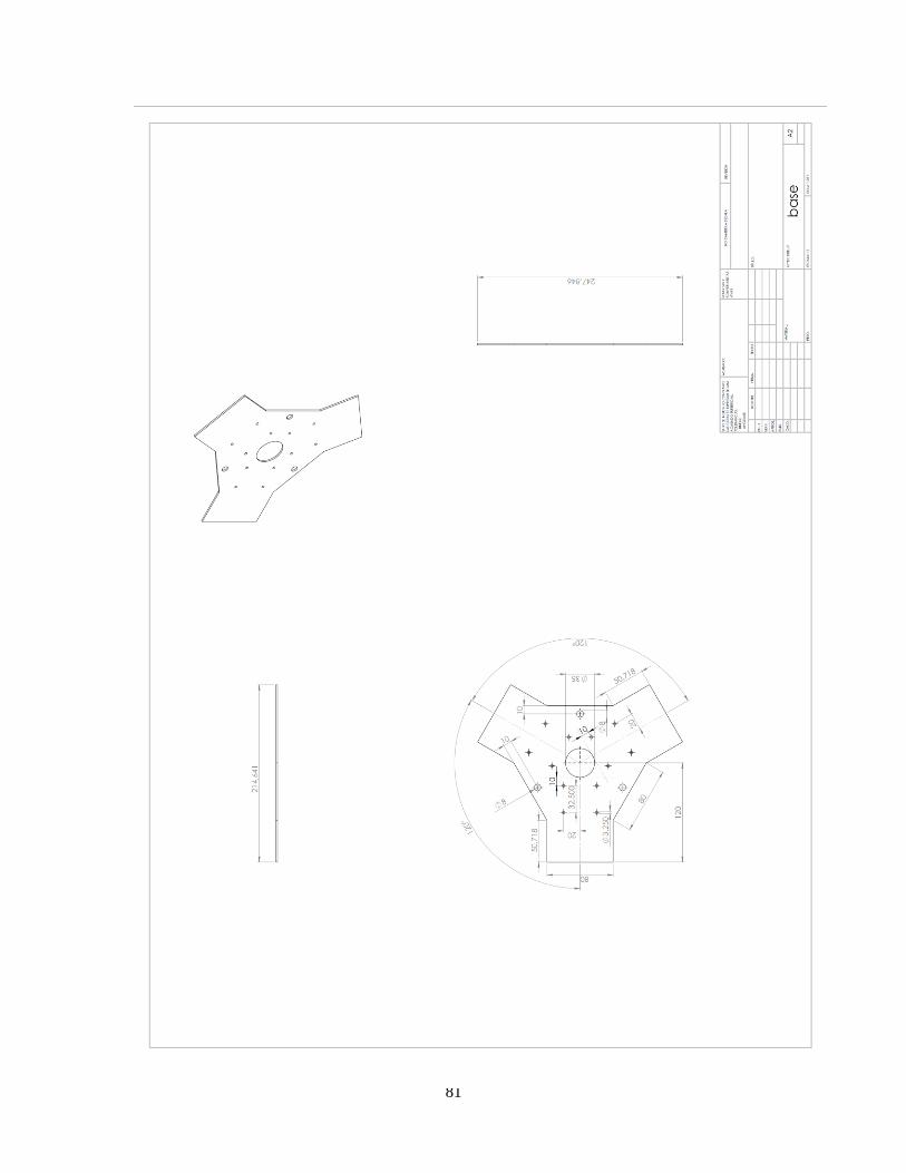
81

82
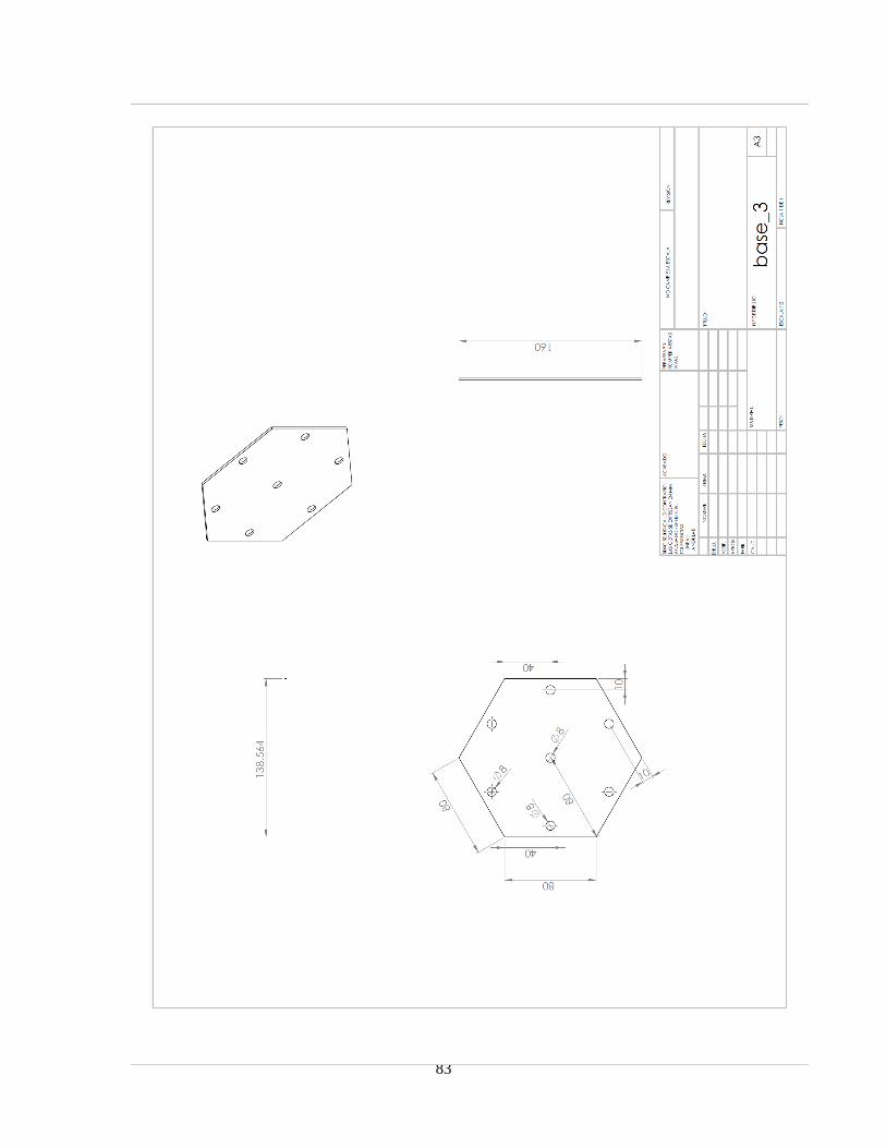
83
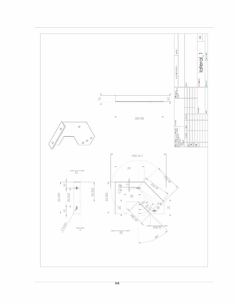
84
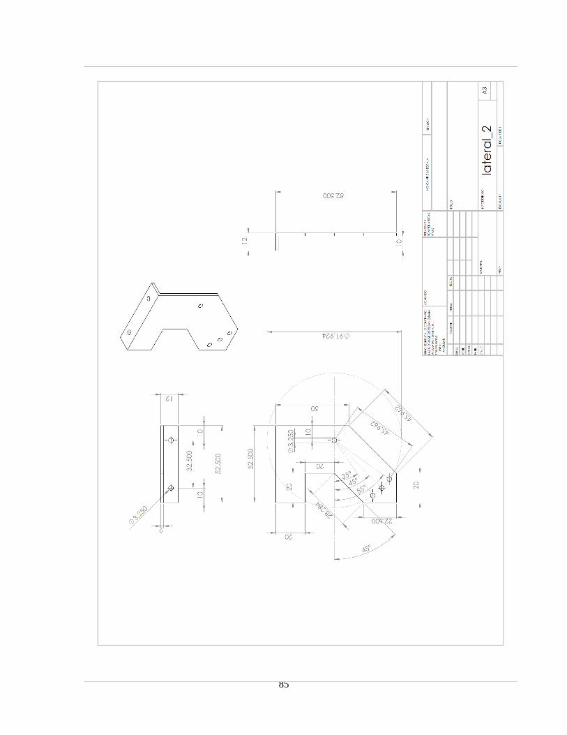
85

86
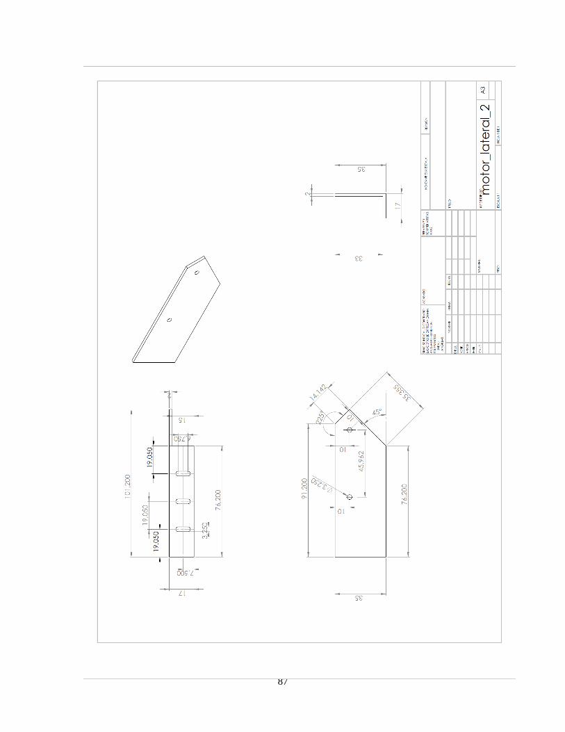
87
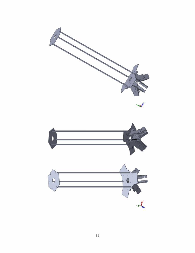
88
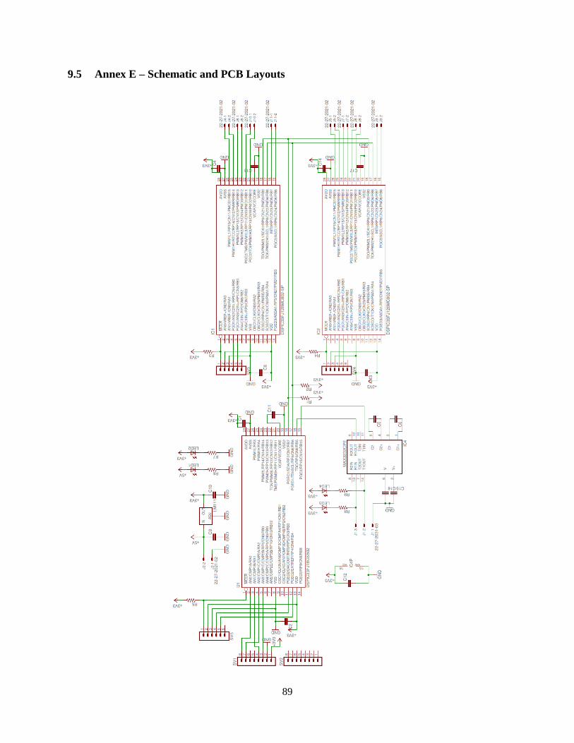
89
9.5 Annex E – Schematic and PCB Layouts
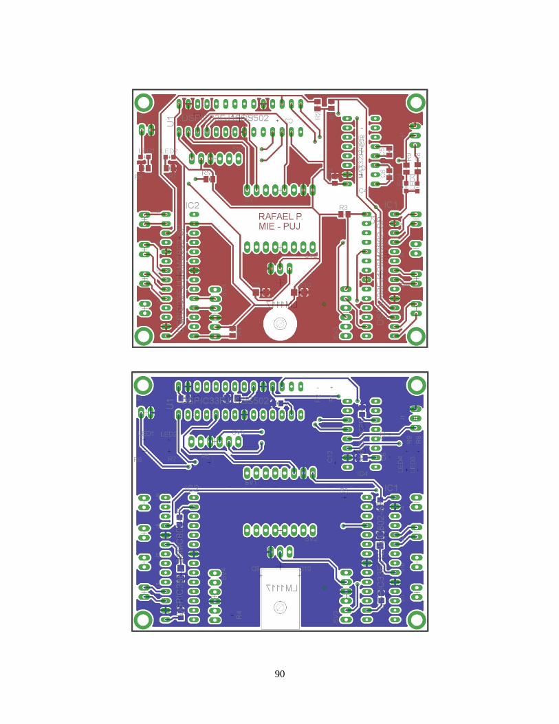
90
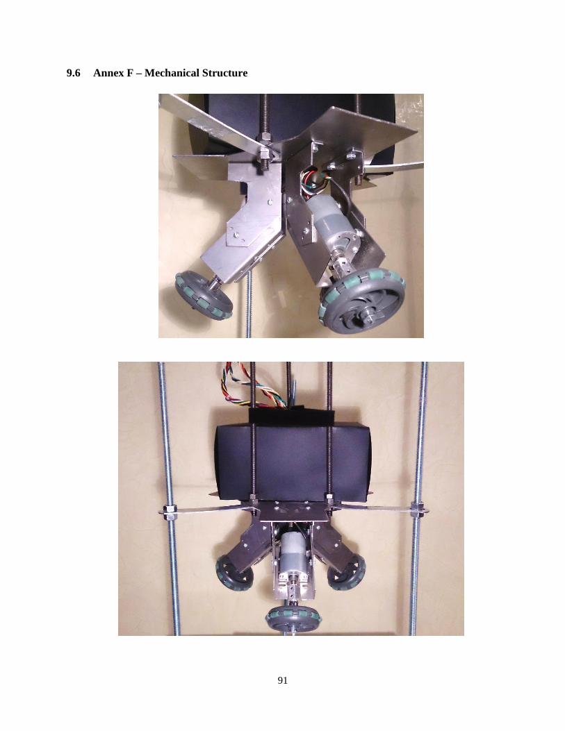
91
9.6 Annex F – Mechanical Structure

92
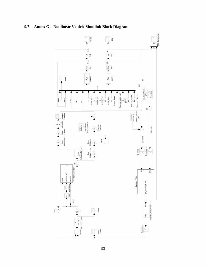
93
9.7 Annex G – Nonlinear Vehicle Simulink Block Diagram
Inp
ut
rb
rad
ius_
ba
ll
mB
ma
ss_
bo
dy
mb
ma
ss_
ba
ll
IB
ine
rtia
_b
od
y
Ib
ine
rtia
_b
all
g
gra
vit
y
l
dis
tan
ce
_b
od
y_
ba
ll
f(u
)
dd
the
ta
f(u
)
dd
ph
i
Vo
lta
ge
Dv
Vis
co
us_
Fri
cti
on
1
j.s+
b
Ve
locit
y/T
orq
ue
To
rqu
e
Th
eta
Sig
n
Sa
tura
tio
n
Qu
an
tize
r1
Qu
an
tize
r
Ph
i_C
om
pa
riso
n
Ph
i
Mo
tor
Su
pp
ly
kt
Ktke
Ke
phi
dphi
phi_
estim
ate
dfc
n
Ka
lma
n_
Fil
ter
1 s
Inte
gra
tor
1/s
Int3
1/s
Int2
1/s
Int1
1/s
Int
Un
ifo
rm
Inp
ut_
No
ise
(Dis
turb
an
ce
s)
Inp
ut
Hyst
ere
sis
-K-
Ge
ar
Re
du
cti
on
^-1
-K-
Ge
ar
Re
du
cti
on
eta
Ge
ar
Eff
icie
ncy1
eta
Ge
ar
Eff
icie
ncy
Ga
uss
ian
Ga
uss
ian
No
ise
dP
hi
Ga
uss
ian
Ga
uss
ian
No
ise
Ph
i
-K-
Eff
ecti
ve
To
rqu
e
In1
Out1
Dis
cre
te_
PID
_C
on
tro
lle
r
1
lm.s
+r
Cu
rre
nt/
Vo
lta
ge
Cu
rre
nt
Dc
Co
ulo
mb
_F
ricti
on
1
torq
ue
thre
sh
old
directio
n
yfc
n
Co
ulo
mb
_F
ricti
on
An
gu
lar
Po
siti
on
|u|
Ab
s
dth
eta
dth
eta
dphi
dphi
dphi
phi
phi
phi
theta
theta
dph
i+n
ois
e
phi+
nois
e