Control and Design ofEngineering Mechanics

Systems

Esubalewe Lakie Yedeg

Licentiate Thesis, May 2013

Department of Computing ScienceUmea UniversitySE-901 87 UmeaSweden

List of Papers

This thesis consists of an introduction to optimal control and topology optimizationproblems and the following two papers:

Paper A Esubalewe Lakie Yedeg and Eddie Wadbro. Optimal ball pitching. In reviewfor Mechanism and Machine Theory.

Paper B Esubalewe Lakie Yedeg, Eddie Wadbro, and Martin Berggren. AnisotropicTopology Optimization of a Reactive Muffler with a Perforated Pipe. Submittedfor publication.

i

ii

Acknowledgement

First of all, I would like to express my deepest respect and most sincere gratitude tomy supervisors Prof. Martin Berggren and Dr. Eddie Wadbro, for offering me theopportunity to carry out my PhD study in the Department of Computing Science, fortheir continuous guidance, invaluable discussion, understanding, and encouragement.Their constructive criticism and excellent advice in this work are highly appreciated.

My deep gratitude also goes to my colleagues and friends for their assistance andgiving me a pleasant working atmosphere.

A very special appreciation goes to my wife Tigist Muluken for her unreservedlove, understanding and encouragement. I thank her for being on my side far awayfrom her parents and giving me a constant support. Finally, I would like to thank myparents and friends in Ethiopia for their support and motivation.

iii

iv

Contents

1 Introduction 1

2 Optimal Control 32.1 Formulation of an optimal control problem . . . . . . . . . . . . . . . 32.2 Numerical Methods . . . . . . . . . . . . . . . . . . . . . . . . . . . . . 4

2.2.1 Indirect methods . . . . . . . . . . . . . . . . . . . . . . . . . . 42.2.2 Direct methods . . . . . . . . . . . . . . . . . . . . . . . . . . . 5

2.3 Discretization . . . . . . . . . . . . . . . . . . . . . . . . . . . . . . . . 62.4 Discrete adjoint based gradient computation . . . . . . . . . . . . . . . 7

3 Summary of Paper A - Optimal Ball Pitching 93.1 Introduction . . . . . . . . . . . . . . . . . . . . . . . . . . . . . . . . . 93.2 Problem formulation . . . . . . . . . . . . . . . . . . . . . . . . . . . . 93.3 Selected numerical results . . . . . . . . . . . . . . . . . . . . . . . . . 12

4 Topology Optimization by Material Distribution 154.1 Problem formulation . . . . . . . . . . . . . . . . . . . . . . . . . . . . 154.2 Discretization . . . . . . . . . . . . . . . . . . . . . . . . . . . . . . . . 164.3 Penalization . . . . . . . . . . . . . . . . . . . . . . . . . . . . . . . . . 174.4 Numerical instabilities and regularization . . . . . . . . . . . . . . . . 18

5 Summary of Paper B - Anisotropic Topology Optimization of a Re-active Muffler with a Perforated Pipe 215.1 Introduction . . . . . . . . . . . . . . . . . . . . . . . . . . . . . . . . . 215.2 Problem description . . . . . . . . . . . . . . . . . . . . . . . . . . . . 215.3 Selected numerical results . . . . . . . . . . . . . . . . . . . . . . . . . 23

v

vi

Chapter 1

Introduction

Many mechanical systems can be modeled by mathematical relations such as ordinarydifferential equations. These systems change with respect to time or any other inde-pendent variable according to the relation. It is often possible to guide these systemsfrom one state to another predefined state by applying some kind of external force orcontrol. It may also be possible to carry out the same task in different ways. If thereare more than one way of performing the task, then it may be possible to choose the“best” way. The best way can be quantified using a measure of performance of thesystem; this measure is often called “cost function”, “objective function”, or “perfor-mance index”. The external force applied to the system corresponding to the bestperformance is called the “optimal” control.

Optimal control also denotes the process of determining control and state trajec-tories for a system over a given period of time to minimize or maximize an objectivefunction. Optimal control is related to the theory of calculus of variations. The the-ory of optimal control has been widely studied and is used in many areas since thebeginning of the so-called “modern” control theory in the 1960s.

In general, control systems are classified into two broad categories: closed loopand open loop systems. In closed-loop systems, also called feedback control systems,the input is affected by the systems output directly or indirectly. It uses the inputand some portion of the output to maintain a prescribed relationship between theoutput and the reference input. However, in open-loop control systems, sometimescalled off-line or non-feedback control systems, the system output does not affect thecontrol input in any form. In this case, the system is free from any change in responseto the output of the process. Standard control theory mostly concerns closed-loopsystems, and these are the ones used in most engineering control applications. Incontrast, the open-loop systems are useful in more special situations. In this thesis,we consider the design of such an open-loop system.

Many mechanical devices play an important role in our daily life. How to “op-timally” design them while satisfying the required system and design constraints isan important engineering concern. The systems can often be modeled by partial dif-ferential equations, such as the equations of elasticity, fluid mechanics, or acoustics.

1

The optimality of the design can be measured by using an objective function thatevaluates for example construction cost, strength of the designed structure, or someother performance measure. If a particular design makes the objective function ashigh or low as possible, depending the objective, it is called an optimal design.

Design optimization of mechanical devices seeks to acquire the best performanceof the structure while satisfying some kind of constraints. Optimal design is becomingmore important due to resource material limitations, the development of computa-tional algorithms, and the availability of high-speed computers. In the last threedecades the subject has developed rapidly with new theoretical insights, computa-tional methods, and application areas. Design optimizations in general can be clas-sified into three main groups, namely, sizing optimization, shape optimization, andtopology optimization.

In sizing optimization, the conceptual geometry of the design is fixed during theoptimization process, and the goal is to find the optimal values of some free parametersof the structure, such as thickness, length, radius, etcetera. In shape optimizationproblems, the shape of the boundaries is subject to optimization but the conceptualdesign is still predetermined. The design variables are some kind of parameterizationof the design boundaries. Topology optimization is the most general and flexibleapproach in structural optimization, where for every point in the design region, itis to be determined whether the point is occupied by a material or not. Thus, thetopology of the structure is not known a priori. Topology optimization can be seenas a generalization of sizing and shape optimization.

In this thesis, we use the optimal control and topology optimization ideas intwo different areas. First we apply the optimal control approach to determine thecontrol of a ball pitching robot in order to throw a ball as far as possible. The open-loop control problem is solved numerically by using Matlab’s fmincon. Then thetopology optimization method is used to determine the internal layout of a reactivemuffler in order to minimize the acoustic energy at the outlet. The Method of MovingAsymptotes is used to solve the optimization problem.

The rest of this comprehensive summary is organized as follows. In Chapter2, a brief introduction to optimal control theory is presented. It is followed by thesummary of Paper A in Chapter 3. Then a short introduction to topology optimizationby material distribution is included in Chapter 4. Finally Chapter 5 presents thesummary of Paper B.

2

Chapter 2

Optimal Control

The subject of optimal control addresses the problem of finding a control input fora given system that optimizes a certain measure, or performance criterion. Optimalcontrol has been under development for many years, and the subject is widely usedin many application areas. Several surveys on the development of optimal controltheory can be found in the literature. Bryson [1] presents the history of optimalcontrol from 1950 to 1985 including the history of calculus of variations since the1600s. A brief historical survey of the development of the calculus of variations andoptimal control is presents by Sargent [2]. He also reviews different approaches to thenumerical solution of optimal control problems. Betts [3] reviews numerical methodsfor trajectory optimization problems. There are several books on the theory of optimalcontrol (for instance Bryson and Ho [4], Hestenes [5], Bryson [6], and Hull [7]). Thenext sections contain a brief introduction to open-loop optimal control problems.

2.1 Formulation of an optimal control problem

A simplified version of the optimal control problem presented in Paper A can beformulated as follows. Given a final time tf , find a control u(t) ∈ Rm that minimizesthe objective function

J(u) = φ(x(tf ), tf ) (2.1)

subject to differential equation

x(t) = f(x(t), u(t), t), t0 ≤ t ≤ tf ,x(t0) = x0,

(2.2)

constraints on the control and state variables

c(x(t), u(t), t) ≤ 0, t0 ≤ t ≤ tf , (2.3)

and terminal conditionψ(x(tf ), tf ) = 0. (2.4)

3

Here, the control and state variables are denoted by u(t) = (u1(t), . . . , um(t))T andx(t) = (x1(t), . . . , xn(t))T , respectively. The functions φ : Rn+1 → R, f : Rn+m+1 →Rn, c : Rn+m+1 → Rl, and ψ : Rn+1 → R are continuously differentiable.

The system of first-order ordinary differential equations (2.2) describes the dy-namics of the system. In control theory, this is called the state-space representationof the system dynamics. Sometimes, the dynamics of the system may depend onhigher order derivatives of the state variable. It is usually convenient to rewrite suchsystems to the state-space form (2.2). An optimal control problem of the above formis known as a Mayer problem.

Remark : A problem with integral cost∫ tft0L((x(t), u(t), t) dt can be formulated in

Mayer form by introducing an additional state variable xL following the dynamics

xL = L((x(t), u(t), t), t0 ≤ t ≤ tf , with xL(t0) = 0.

2.2 Numerical Methods

For some optimal control problems, it is possible to obtain analytical solutions fromthe necessary and sufficient optimality conditions [8, 9, 10]. However, optimal controlproblems are typically non-linear and do not possess analytical solutions in most cases.Hence, it is in general necessary to employ numerical methods to solve optimal controlproblems. Numerical methods for optimal control problems are generally classifiedinto indirect methods and direct methods [3, 11].

2.2.1 Indirect methods

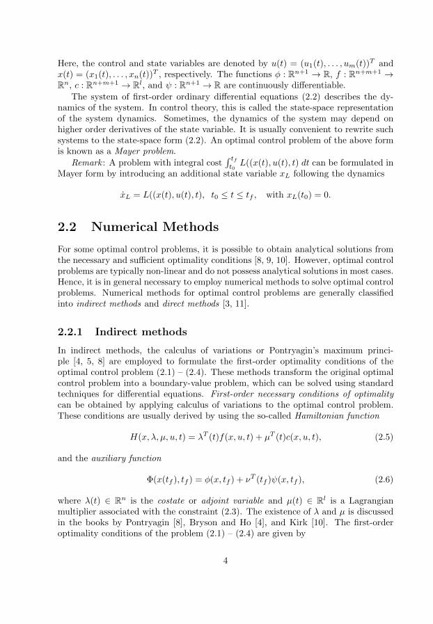
In indirect methods, the calculus of variations or Pontryagin’s maximum princi-ple [4, 5, 8] are employed to formulate the first-order optimality conditions of theoptimal control problem (2.1) – (2.4). These methods transform the original optimalcontrol problem into a boundary-value problem, which can be solved using standardtechniques for differential equations. First-order necessary conditions of optimalitycan be obtained by applying calculus of variations to the optimal control problem.These conditions are usually derived by using the so-called Hamiltonian function

H(x, λ, µ, u, t) = λT (t)f(x, u, t) + µT (t)c(x, u, t), (2.5)

and the auxiliary function

Φ(x(tf ), tf ) = φ(x, tf ) + νT (tf )ψ(x, tf ), (2.6)

where λ(t) ∈ Rn is the costate or adjoint variable and µ(t) ∈ Rl is a Lagrangianmultiplier associated with the constraint (2.3). The existence of λ and µ is discussedin the books by Pontryagin [8], Bryson and Ho [4], and Kirk [10]. The first-orderoptimality conditions of the problem (2.1) – (2.4) are given by

4

λ = −∂H∂x

= −λT ∂f∂x− µT ∂c

∂x, (2.7)

0 =∂H

∂u= λT

∂f

∂u+ µT

∂c

∂u, (2.8)

and

λ(tf ) =∂Φ

∂x|t=tf , (

∂Φ

∂t+H)|t=tf = 0, (2.9)

in addition to state equation (2.2), constraint (2.3), terminal condition (2.4), and thecomplementary slackness conditions

µici = 0, i = 1 . . . l. (2.10)

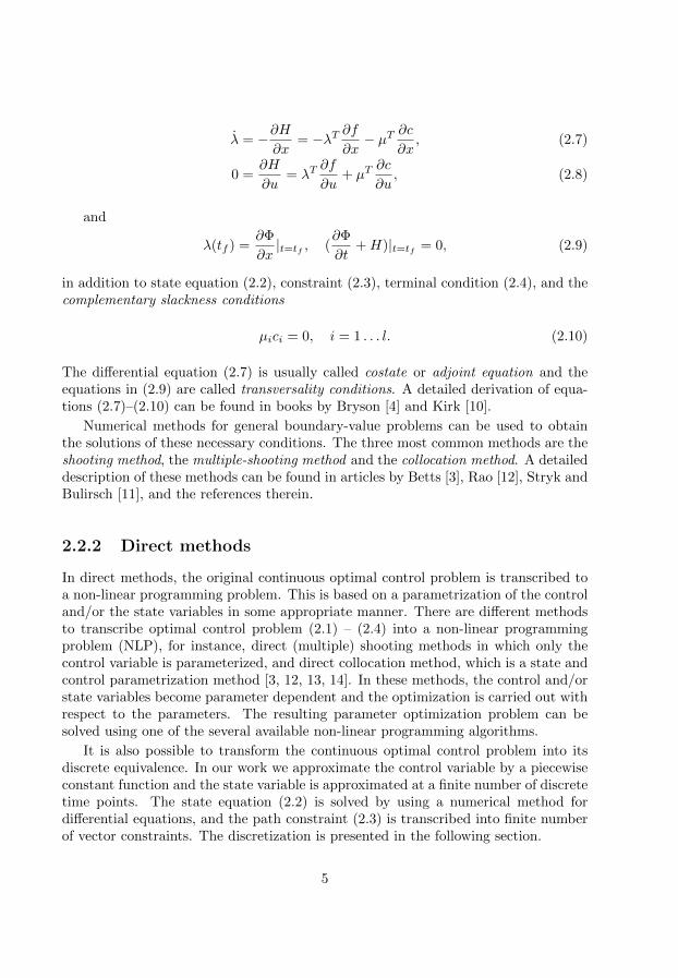
The differential equation (2.7) is usually called costate or adjoint equation and theequations in (2.9) are called transversality conditions. A detailed derivation of equa-tions (2.7)–(2.10) can be found in books by Bryson [4] and Kirk [10].

Numerical methods for general boundary-value problems can be used to obtainthe solutions of these necessary conditions. The three most common methods are theshooting method, the multiple-shooting method and the collocation method. A detaileddescription of these methods can be found in articles by Betts [3], Rao [12], Stryk andBulirsch [11], and the references therein.

2.2.2 Direct methods

In direct methods, the original continuous optimal control problem is transcribed toa non-linear programming problem. This is based on a parametrization of the controland/or the state variables in some appropriate manner. There are different methodsto transcribe optimal control problem (2.1) – (2.4) into a non-linear programmingproblem (NLP), for instance, direct (multiple) shooting methods in which only thecontrol variable is parameterized, and direct collocation method, which is a state andcontrol parametrization method [3, 12, 13, 14]. In these methods, the control and/orstate variables become parameter dependent and the optimization is carried out withrespect to the parameters. The resulting parameter optimization problem can besolved using one of the several available non-linear programming algorithms.

It is also possible to transform the continuous optimal control problem into itsdiscrete equivalence. In our work we approximate the control variable by a piecewiseconstant function and the state variable is approximated at a finite number of discretetime points. The state equation (2.2) is solved by using a numerical method fordifferential equations, and the path constraint (2.3) is transcribed into finite numberof vector constraints. The discretization is presented in the following section.

5

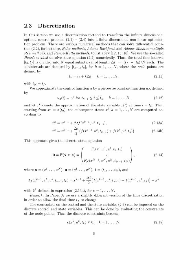
2.3 Discretization

In this section we use a discretization method to transform the infinite dimensionaloptimal control problem (2.1) – (2.4) into a finite dimensional non-linear optimiza-tion problem. There are various numerical methods that can solve differential equa-tion (2.2), for instance, Euler methods, Adams-Bashforth and Adams-Moulton multiple-step methods, and Runge-Kutta methods, to list a few [12, 15, 16]. We use the so-calledHeun’s method to solve state equation (2.2) numerically. Thus, the total time interval[t0, tf ] is divided into N equal subinterval of length ∆t = (tf − t0)/N each. Thesubintervals are denoted by [tk−1, tk], for k = 1, . . . , N , where the node points aredefined by

tk = t0 + k∆t, k = 1, . . . , N, (2.11)

with tN = tf .We approximate the control function u by a piecewise constant function ud, defined

by

ud(t) = uk for tk−1 ≤ t ≤ tk, k = 1, . . . , N, (2.12)

and let xk denote the approximation of the state variable x(t) at time t = tk. Thenstarting from x0 = x(t0), the subsequent states xk, k = 1, . . . , N are computed ac-cording to

xk = xk−1 + ∆tf(xk−1, uk, tk−1), (2.13a)

xk = xk−1 +∆t

2

(f(xk−1, uk, tk−1) + f(xk, uk, tk)

). (2.13b)

This approach gives the discrete state equation

0 = F(x,u, t) =

F1(x0, x1, u1, t0, t1)...

FN (xN−1, xN , uN , tN−1, tN )

, (2.14)

where x = (x1, . . . , xN ), u = (u1, . . . , uN ), t = (t1, . . . , tN ), and

Fk(xk−1, xk, uk, tk−1, tk) = xk−1 +∆t

2

(f(xk−1, uk, tk−1) + f(xk−1, uk, tk)

)− xk

with xk defined in expression (2.13a), for k = 1, . . . , N .Remark : In Paper A we use a slightly different version of the time discretization

in order to allow the final time tf to change.The constraints on the control and the state variables (2.3) can be imposed on the

discrete control and state variables. This can be done by evaluating the constraintsat the node points. Thus the discrete constraints become

c(xk, uk, tk) ≤ 0, k = 1, . . . , N. (2.15)

6

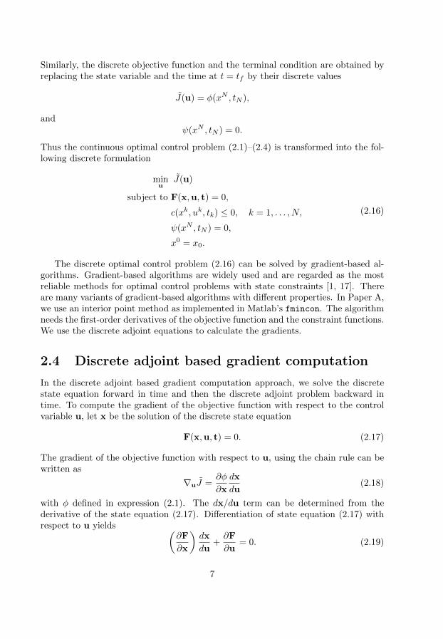
Similarly, the discrete objective function and the terminal condition are obtained byreplacing the state variable and the time at t = tf by their discrete values

J(u) = φ(xN , tN ),

andψ(xN , tN ) = 0.

Thus the continuous optimal control problem (2.1)–(2.4) is transformed into the fol-lowing discrete formulation

minu

J(u)

subject to F(x,u, t) = 0,

c(xk, uk, tk) ≤ 0, k = 1, . . . , N,

ψ(xN , tN ) = 0,

x0 = x0.

(2.16)

The discrete optimal control problem (2.16) can be solved by gradient-based al-gorithms. Gradient-based algorithms are widely used and are regarded as the mostreliable methods for optimal control problems with state constraints [1, 17]. Thereare many variants of gradient-based algorithms with different properties. In Paper A,we use an interior point method as implemented in Matlab’s fmincon. The algorithmneeds the first-order derivatives of the objective function and the constraint functions.We use the discrete adjoint equations to calculate the gradients.

2.4 Discrete adjoint based gradient computation

In the discrete adjoint based gradient computation approach, we solve the discretestate equation forward in time and then the discrete adjoint problem backward intime. To compute the gradient of the objective function with respect to the controlvariable u, let x be the solution of the discrete state equation

F(x,u, t) = 0. (2.17)

The gradient of the objective function with respect to u, using the chain rule can bewritten as

∇uJ =∂φ

∂x

dx

du(2.18)

with φ defined in expression (2.1). The dx/du term can be determined from thederivative of the state equation (2.17). Differentiation of state equation (2.17) withrespect to u yields (

∂F

∂x

)dx

du+∂F

∂u= 0. (2.19)

7

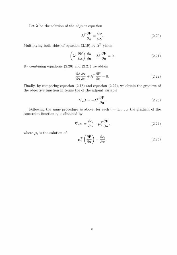
Let λ be the solution of the adjoint equation

λT∂F

∂x=∂φ

∂x. (2.20)

Multiplying both sides of equation (2.19) by λT yields

(λT

∂F

∂x

)dx

du+ λT

∂F

∂u= 0. (2.21)

By combining equations (2.20) and (2.21) we obtain

∂φ

∂x

dx

du+ λT

∂F

∂u= 0. (2.22)

Finally, by comparing equation (2.18) and equation (2.22), we obtain the gradient ofthe objective function in terms the of the adjoint variable

∇uJ = −λT ∂F

∂u. (2.23)

Following the same procedure as above, for each i = 1, . . . , l the gradient of theconstraint function ci is obtained by

∇uci =∂ci∂u− µTi

∂F

∂u, (2.24)

where µi is the solution of

µTi

(∂F

∂x

)=∂ci∂x

. (2.25)

8

Chapter 3

Summary of Paper A - Optimal Ball

Pitching

3.1 Introduction

In Paper A, we study an optimal control problem of a ball pitching robot that isdesigned to capture important dynamics of the human upper limb (including theshoulder, arm, and forearm) during an overarm throw. The robot has two links thatare connected at the elbow joint by a linear torsional spring. The links represent thearm and forearm, and the spring represents the stiffness of the muscles around theelbow joint in human upper limb [18, 19]. The two-link robot is connected to a motorshaft at the shoulder joint by a non-linear torsional spring. At the end of the forearm,the robot is equipped with a gripping mechanism that allows the robot to grasp andrelease the ball at any required time.

The main objective is to determine the optimal motor torque and the release timethat enable the robot to pitch the ball as far as possible. We include constraints onthe motor torque and power as well as the angular velocity of the motor shaft intothe problem formulation. For computational efficiency, we replace the time-globalconstraints on maximum allowed power and maximum angular velocity of the motorshaft by approximations based on integral quantities.

3.2 Problem formulation

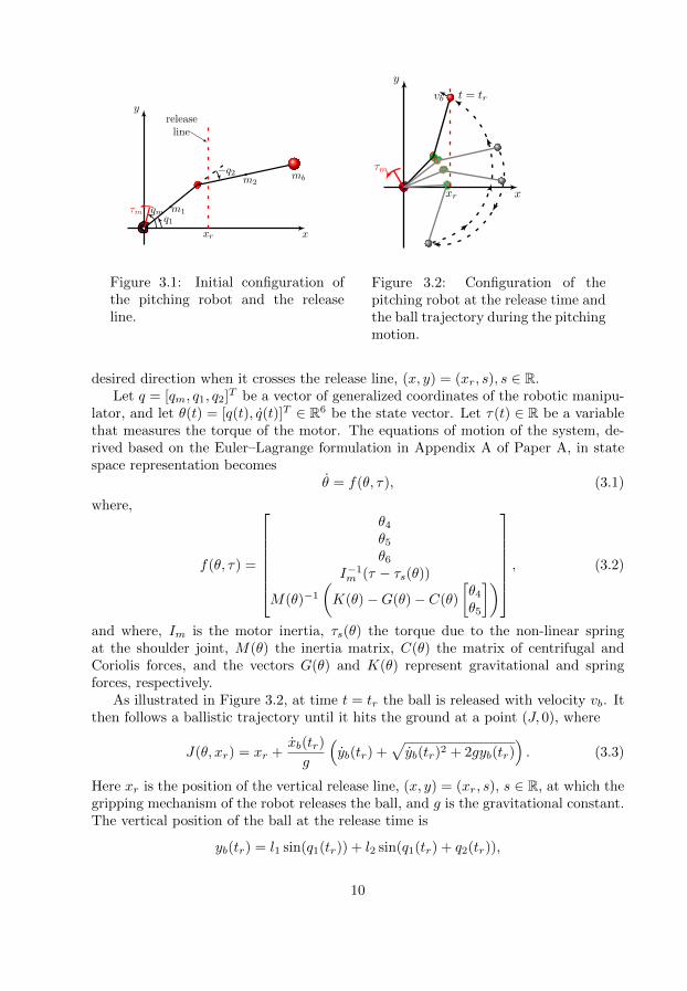
The initial configuration of the two-link robot with a gripping mechanism holding aball is illustrated in Figure 3.1. We denote the two links by the arm and forearm,respectively. Let q2 measure the angle change between the arm and the forearm atthe elbow joint. The angles q1 and qm, measured with respect to the horizontal axis,describe the configuration of the arm and the motor shaft, respectively. The onlydriving force of the system comes from the motor shaft. Figure 3.2 shows a trajectoryof the ball during a pitching motion. The ball gets released with velocity vb in the

9

x

y

m1

m2

xr

releaseline

qmq1

−q2

τm

mb

1Figure 3.1: Initial configuration ofthe pitching robot and the releaseline.

x

y

xr

t = trvb

τm

1Figure 3.2: Configuration of thepitching robot at the release time andthe ball trajectory during the pitchingmotion.

desired direction when it crosses the release line, (x, y) = (xr, s), s ∈ R.Let q = [qm, q1, q2]T be a vector of generalized coordinates of the robotic manipu-

lator, and let θ(t) = [q(t), q(t)]T ∈ R6 be the state vector. Let τ(t) ∈ R be a variablethat measures the torque of the motor. The equations of motion of the system, de-rived based on the Euler–Lagrange formulation in Appendix A of Paper A, in statespace representation becomes

θ = f(θ, τ), (3.1)

where,

f(θ, τ) =

θ4

θ5

θ6

I−1m (τ − τs(θ))

M(θ)−1

(K(θ)−G(θ)− C(θ)

[θ4

θ5

])

, (3.2)

and where, Im is the motor inertia, τs(θ) the torque due to the non-linear springat the shoulder joint, M(θ) the inertia matrix, C(θ) the matrix of centrifugal andCoriolis forces, and the vectors G(θ) and K(θ) represent gravitational and springforces, respectively.

As illustrated in Figure 3.2, at time t = tr the ball is released with velocity vb. Itthen follows a ballistic trajectory until it hits the ground at a point (J, 0), where

J(θ, xr) = xr +xb(tr)

g

(yb(tr) +

√yb(tr)2 + 2gyb(tr)

). (3.3)

Here xr is the position of the vertical release line, (x, y) = (xr, s), s ∈ R, at which thegripping mechanism of the robot releases the ball, and g is the gravitational constant.The vertical position of the ball at the release time is

yb(tr) = l1 sin(q1(tr)) + l2 sin(q1(tr) + q2(tr)),

10

where l1 and l2 are the lengths of the arm and the forearm, respectively. Similarly,the velocity of the ball vb = (xb, yb) at time t = rr is given by

xb(tr) = −l1 sin(q1(tr))q1(tr)− l2 sin(q1(tr) + q2(tr))(q1(tr) + q2(tr)),

yb(tr) = l1 cos(q1(tr))q1(tr) + l2 cos(q1(tr) + q2(tr))(q1(tr) + q2(tr)).

Note that the robot’s shoulder is held fixed at the origin of the coordinate system andthat the ball has thrown in the negative x direction. Hence, minimizing J impliesmaximizing the distance between the origin and the point (J, 0).

We minimize J over the torque change in time. By inclusion of the constraints onthe motor torque and torque change in the set of admissible controls we obtain

A =

η ∈ L∞ | sup

t|η(t)| ≤ Cτ , sup

t

∣∣∣∣τ0 +

∫ t

0

η(s) ds

∣∣∣∣ ≤ τ, (3.4)

where τ is the maximum allowed torque of the motor, Cτ is the bound on the torquechange in time, and η is the our control function defined by

τ = η,

τ(0) = τ0.(3.5)

For computational efficiency, we replace the time-global constraints on maximumallowed power and maximum angular velocity of the motor shaft by approximationsbased on integral quantities (see Paper A for the discussion). For practical reasons,we impose the constraint |xr| ≤ L on the release line, where L = l1 + l2. Since it ispossible to determine the release line position if the release time is known and viceversa, we optimize with respect to the release line position instead of the time.

Putting the system dynamics, the objective function, and the constraints together,we obtain the optimal control problem

minη∈A,|xr|≤L

J(xr, θ(tr))

subject to τ = η, τ(0) = τ0,

θ = f(θ, τ), θ(0) = θ(0),(

1

tr

∫ tr

0

|θ4|p dt

)1/p

≤(

1

p+ 1

)1/p

Qmax,

(1

tr

∫ tr

0

|τθ4|p dt

)1/p

≤(

1

p+ 1

)1/p

Pmax,

(3.6)

where Qmax and Pmax are the maximum allowed angular velocity of the motor shaftand input power of the motor, respectively, and θ(0) is the initial state of the system.

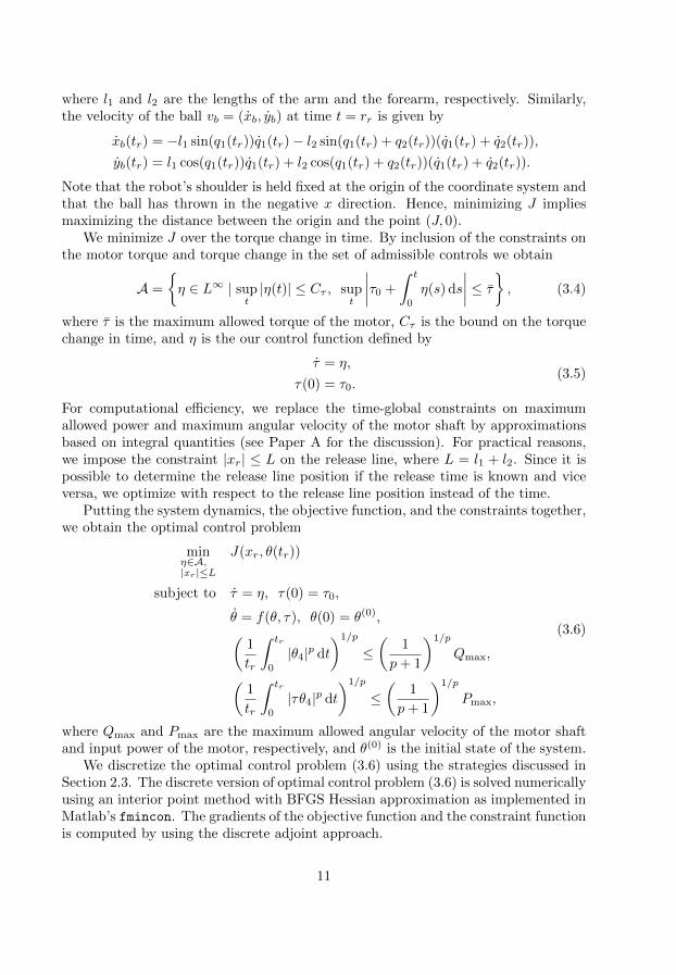
We discretize the optimal control problem (3.6) using the strategies discussed inSection 2.3. The discrete version of optimal control problem (3.6) is solved numericallyusing an interior point method with BFGS Hessian approximation as implemented inMatlab’s fmincon. The gradients of the objective function and the constraint functionis computed by using the discrete adjoint approach.

11

0 0.2 0.4 0.6 0.8−50

0

50

100

Time [s]

Moto

rto

rque[N

m]

−0.5 0 0.5 1−0.6

−0.4

−0.2

0

0.2

0.4

0.6

0.8

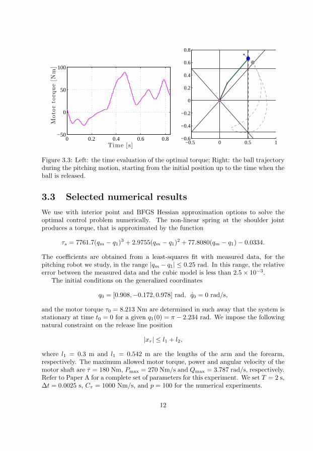
Figure 3.3: Left: the time evaluation of the optimal torque; Right: the ball trajectoryduring the pitching motion, starting from the initial position up to the time when theball is released.

3.3 Selected numerical results

We use with interior point and BFGS Hessian approximation options to solve theoptimal control problem numerically. The non-linear spring at the shoulder jointproduces a torque, that is approximated by the function

τs = 7761.7(qm − q1)3 + 2.9755(qm − q1)2 + 77.8080(qm − q1)− 0.0334.

The coefficients are obtained from a least-squares fit with measured data, for thepitching robot we study, in the range |qm − q1| ≤ 0.25 rad. In this range, the relativeerror between the measured data and the cubic model is less than 2.5× 10−3.

The initial conditions on the generalized coordinates

q0 = [0.908,−0.172, 0.978] rad, q0 = 0 rad/s,

and the motor torque τ0 = 8.213 Nm are determined in such away that the system isstationary at time t0 = 0 for a given q1(0) = π − 2.234 rad. We impose the followingnatural constraint on the release line position

|xr| ≤ l1 + l2,

where l1 = 0.3 m and l1 = 0.542 m are the lengths of the arm and the forearm,respectively. The maximum allowed motor torque, power and angular velocity of themotor shaft are τ = 180 Nm, Pmax = 270 Nm/s and Qmax = 3.787 rad/s, respectively.Refer to Paper A for a complete set of parameters for this experiment. We set T = 2 s,∆t = 0.0025 s, Cτ = 1000 Nm/s, and p = 100 for the numerical experiments.

12

0 0.2 0.4 0.6 0.8

−2

−1

0

1

Time [s]

Angle

[rad]

qm q1 q2

0 0.2 0.4 0.6 0.8−20

−10

0

10

Time [s]

Angularvelo

city[rad/s]

qm q1 q2

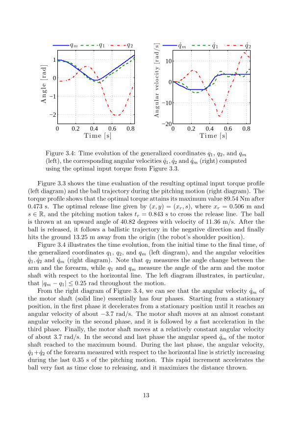
Figure 3.4: Time evolution of the generalized coordinates q1, q2, and qm(left), the corresponding angular velocities q1, q2 and qm (right) computedusing the optimal input torque from Figure 3.3.

Figure 3.3 shows the time evaluation of the resulting optimal input torque profile(left diagram) and the ball trajectory during the pitching motion (right diagram). Thetorque profile shows that the optimal torque attains its maximum value 89.54 Nm after0.473 s. The optimal release line given by (x, y) = (xr, s), where xr = 0.506 m ands ∈ R, and the pitching motion takes tr = 0.843 s to cross the release line. The ballis thrown at an upward angle of 40.82 degrees with velocity of 11.36 m/s. After theball is released, it follows a ballistic trajectory in the negative direction and finallyhits the ground 13.25 m away from the origin (the robot’s shoulder position).

Figure 3.4 illustrates the time evolution, from the initial time to the final time, ofthe generalized coordinates q1, q2, and qm (left diagram), and the angular velocitiesq1, q2 and qm (right diagram). Note that q2 measures the angle change between thearm and the forearm, while q1 and qm measure the angle of the arm and the motorshaft with respect to the horizontal line. The left diagram illustrates, in particular,that |qm − q1| ≤ 0.25 rad throughout the motion.

From the right diagram of Figure 3.4, we can see that the angular velocity qm ofthe motor shaft (solid line) essentially has four phases. Starting from a stationaryposition, in the first phase it decelerates from a stationary position until it reaches anangular velocity of about −3.7 rad/s. The motor shaft moves at an almost constantangular velocity in the second phase, and it is followed by a fast acceleration in thethird phase. Finally, the motor shaft moves at a relatively constant angular velocityof about 3.7 rad/s. In the second and last phase the angular speed qm of the motorshaft reached to the maximum bound. During the last phase, the angular velocity,q1+q2 of the forearm measured with respect to the horizontal line is strictly increasingduring the last 0.35 s of the pitching motion. This rapid increment accelerates theball very fast as time close to releasing, and it maximizes the distance thrown.

13

14

Chapter 4

Topology Optimization by Material

Distribution

Topology optimization is a mathematical approach that optimizes the material layoutof a device within a given design space such that a certain performance criterion ismaximized or minimized for a given set of conditions. Starting from the publication ofthe pioneering paper by Bendsøe and Kikuchi [20], topology optimization methods forcontinuum structures have been expanded significantly and applied to many practicalengineering problems. Topology optimization has been used starting from designingmaterials at micro-level (example Sigmund [21], Zhou and Li [22], and Jensen etal. [23]) to large-scale designs such as bridges and buildings, and for components withinthe automobile and aircraft industries (example Borrvall and Petersson [24], Guan etal. [25], Wang et al. [26], and Krog et al. [27]). The area of topology optimization isdominated by methods that apply the material distribution concept. Most numericalmethods for topology optimization are based on finite element methods. In this case,the design domain is discretized into a fine mesh of elements, and the purpose of thealgorithm is to find the optimal material distribution by determining for each elementin the design domain whether it should be filled with material (solid element) or not(element with air). In the next sections, a brief overview on topology optimizationby the material distribution method is introduced.

4.1 Problem formulation

In general, a topology optimization problem consists of an objective function, a designdomain, a design constraint, and a state equation. Let Ω be the design domain andΩm ⊂ Ω the region in the design domain occupied by solid material. The distributionof material in Ω is usually modeled by using a material indicator function α, defined asα(x) = 1, if x ∈ Ωm and α(x) = 0 otherwise. Mathematically, a topology optimization

15

problem in its general form is given by

minα∈U

J(α, u) (4.1a)

s.t. a(α;u, v) = `(v), ∀v ∈ V, (4.1b)

C(α, u) ≤ 0, (4.1c)

where U = α : α(x) ∈ 0, 1, x ∈ Ω is the set of admissible designs, J is an objectivefunction to measure the performance, u denotes the state variable, C is a constraintfunction, and V is an appropriate functional space. The design and the state variablesare related by the state equation, in this case given by the variational form (4.1b).

Remark : In acoustic related topology optimization problems the material indicatorfunction α is 1 in region of air and 0 in the region which is occupied by sound-hardmaterial.

The prototype problem of this kind is the classical problem of minimizing thecompliance, J = `(u) (equivalent to maximizing the stiffness), of a mechanical struc-ture subject to state equation (4.1b), the governing equation of linear elasticity, andthe volume constraint, C(α) =

∫Ωα(x)dx − V ≤ 0. Here, V is the upper bound

of the volume occupied by solid material. In order to guarantee coercivity of thebilinear form, the material indicator function should not be zero. Therefore, thespace of admissible designs U = α : α(x) ∈ 0, 1, x ∈ Ω is usually replaced byU = α : α(x) ∈ ε, 1, x ∈ Ω for a small constant ε > 0, such that α(x) = ε forx ∈ Ω− Ωm.

In many cases, topology optimization problems of the form (4.1) are ill-posed.Typically, the ill-posedness is due to the existence of a sequence of minimizers thatdo not converge [28], which, after discretization, manifests itself as mesh dependencyin the numerical solution. A relaxation method can be used to address this problem.It also allows the use of gradient-based optimization algorithms. By letting α takevalues in the continuous range [ε, 1], the binary optimization problem (4.1) becomes

minα∈U

J(α, u), (4.2a)

s.t. a(α;u, v) = `(v), ∀v ∈ V, (4.2b)

C(α, u) ≤ 0, (4.2c)

where U = α : ε ≤ α(x) ≤ 1, x ∈ Ω.In the case of compliance minimization, there exist a unique solution of prob-

lem (4.2). The proof of the existence of a solution can be found in Section 5.2 of thebook [29] by Bendsøe and Sigmund.

4.2 Discretization

Numerical methods are typically used to obtain an approximate solution of optimiza-tion problem (4.2). Following a finite element procedure, the domain Ω is partitioned

16

into N small subdomains called elements Ek, k = 1, . . . , N , such that Ω = ∪Nk=1Ek.The material indicator function α is approximated by αh, an element-wise constantfunction. The state variable u is approximated by uh ∈ Vh(Ω), where Vh ⊂ V isthe space of continuous and element-wise polynomial functions. The discrete statevariable uh is the solution of the discrete state equation for a given feasible design αh

ah(αh;uh, vh) = `h(vh), ∀vh ∈ Vh, (4.3)

where vh, ah and `h are the discretized version of v, a and `, respectively. Similarly,the objective and constraint functions are replaced by their corresponding discreteversion.

Then the discrete version of the optimization problem (4.2) can be formulated as

minαh∈Uh

Jh(αh, uh)

s.t. ah(αh;uh, vh) = `h(vh), ∀vh ∈ Vh,Ch(αh, uh) ≤ 0,

(4.4)

where Jh and Ch are the discrete version of the objective and constraint functions,and the space of admissible designs, Uh is the set of element-wise constant functions.There are different optimization methods to solve the optimization problem (4.4), forinstance, the optimality criteria method [30] and the Method of Moving Asymptotes(MMA) [31]. The MMA method is well suited mathematical algorithm for topologyoptimization problems [29]. We use the MMA to solve the topology optimizationproblem in Paper B.

4.3 Penalization

Unfortunately, the relaxed problem (4.2) is different from the original binary prob-lem (4.1), and the material indicator function corresponding to the relaxed problemis usually not binary. This results in “gray” regions in the optimized designs. How-ever, the goal of the original problem is to find a black and white structure, that is,a solution α such that α(x) is either ε or 1 for all points x ∈ Ω. To obtain binaryoptimal designs, it is common to introduce some kind of penalization to force theintermediate values towards either ε or 1.

There are different penalization methods in topology optimization. One of themethods, commonly used in acoustic related problems, deals with the intermediatevalues by adding a penalty function Jp to the objective function (4.2a), and optimizesthe penalized problem

minα∈U

J(α, u) + γJp(α) (4.5a)

s.t. a(α;u, v) = `(v), ∀v ∈ V, (4.5b)

C(α, u) ≤ 0. (4.5c)

17

Alternatively, the penalty function can be added as a constraint by including

Jp(α) ≤ εp,

in the problem (4.2), for a small positive number εp. One of the frequently usedpenalty functions [32, 33], is

Jp(α) =

∫

Ω

(1− α)(α− ε). (4.6)

For topology optimization problems with active volume constraint, the so calledSolid Isotropic Material with Penalization (SIMP) method is widely used. It wassuggested by Bendsøe [34] and uses a non-linear interpolation function of the form

fq(α) = αq, (4.7)

where q > 1 is a constant, together with the volume constraint∫

Ω

α(x)dx ≤ V. (4.8)

In this method, as the value of q increases the local stiffness of the intermediate valuesdecreases while their volume are unchanged. An alternating approach to the SIMPmethod is RAMP (Rational Approximation of Material Properties)

fq(α) =α

1 + q(1− α), (4.9)

with q > 0, which was introduced by Rietz [35] and analyzed by Stolpe and Svan-berg [36]. In these cases, the parameter q represents the amount of penalization, andthe variational equation in problem (4.2) is replaced by

a(fq(α);u, v) = `(v), ∀v ∈ V,

with volume constraint (4.8).

4.4 Numerical instabilities and regularization

A well-organized survey of numerical instabilities in topology optimization for con-tinuum elastic structures and their corresponding regularization methods is given bySigmund and Petersson [28]. In this section, a brief overview of numerical instabili-ties and a possible treatment method is presented. In general the common numericalproblems arising in topology optimization can be categorized in to three groups: meshdependency, formation of checkerboard pattern, and local minima.

Mesh dependency is the problem of finding qualitatively different solutions withmore and more holes and finer structural elements with better results when the prob-lem is solved using the same algorithm but with finer and finer mesh sizes. It is related

18

to the non-existence of solution to the optimization problem, due to non-closednessof the set of feasible designs.

A checkerboard pattern is the occurrence of high oscillations of the design variablebetween air and material. The issue is usually associated with the choice of finiteelements and can often be prevented by using higher-order finite element for the statevariable [37].

Most problems in topology optimization are not convex and many of them havemultiple (local) minima [29]. Hence, performing the same numerical optimizationalgorithm but with a small change in the starting guess or algorithmic parameterscan result different locally optimal solutions. Based on experience, a continuationapproach is suggested to overcome this problem [28, 29]. This approach lets the pe-nalization parameters increase or decrease gradually in order to guide the developmentof the solution towards reliably good designs.

In the literature, several methods are proposed to tackle the problems with checker-board patterns and mesh-dependency in topology optimization [28, 29, 34]. Mesh-independent filtering methods are among the most common such methods due totheir ease of implementation and their efficiency [38]. The use of filtering in topol-ogy optimization, based on ideas borrowed from image processing, was suggested bySigmund [39]. Since then, filters have been used in order to regularize many topol-ogy optimization problems [33, 40, 41, 42]. Filtering methods engaged to regularizetopology optimization problems can be grouped into density and sensitivity basedmethods.

Density filtering was introduced by Bruns and Tortorelli [40]. The main idea isto modify the element density such that it depends on the densities of elements ina predefined neighborhood. The problem is optimized with respect to an artificialdensity variable α and the physical density, the filtered one, is achieved by using aconvolution of a filter kernel and the artificial density variable, given by

α(x) =

∫

Rd

φ(x, y)α(y)dy, (4.10)

where d is the space dimenstion. The filer kernel φ, typical in topology optimization,is

φ(x, y) = σ(x) max

(0, 1− |x− y|

τ

), (4.11)

where τ > 0 is the filter radius and σ(x) is a normalization factor such that

∫

Rd

φ(x, y)dy = 1.

Bourdin [41] proved the existence as well as finite element convergence of theminimum compliance problem using this filter and the SIMP penalization method.In Paper B, we use density filtering with an anisotropic generalization of integrationkernel (4.11). The filtered version of the topology optimization problem (4.2) is given

19

byminα∈U

J(α, u),

s.t. α(·) =

∫

Rd

φ(·, y)α(y)dy

a(α;u, v) = `(v), ∀v ∈ V,C(α, u) ≤ 0.

(4.12)

The other alternative, sensitivity filtering, is used to modify the design sensitivityof a particular element by making it dependent on a weighted average over its neigh-boring elements. In this method, the design updates are performed using the filteredsensitivity instead of the real sensitivity. It is a simple approach to use but risky too,especially for line-search based optimization algorithms [38]. Different variations ofthe two filtering methods are reviewed in Sigmund’s article [38]. Alternative tech-niques that could be used to produce black and white solutions are presented in thesurvey article [28] by Sigmund and Petersson.

20

Chapter 5

Summary of Paper B - Anisotropic

Topology Optimization of a Reactive

Muffler with a Perforated Pipe

5.1 Introduction

In Paper B, we consider the optimal design of a reactive muffler. A reactive muffleris a device commonly used to attenuate exhaust noise of internal combustion engines.It consists of a series of chambers of different dimensions connected together to causeimpedance mismatch, that is, to reflect a substantial part of the acoustic energyback to the source or back and forth among the chambers [43]. Any change on thearrangement or dimensions of the muffler components affect the performance.

We used topology optimization by material distribution to optimize the internalconfiguration of an expansion chamber in a cylindrical symmetric reactive muffler.The objective is to reduce the outgoing acoustic energy at the outlet as much aspossible by distributing sound hard material inside the expansion chamber to reflectsome part of the acoustic energy back to the source. The propagation of acoustic wavesin the muffler is modeled by the Helmholtz equation, and a finite element method isused to discretize the equation. The Method of Moving Asymptotes, MMA [31] isused to solve the topology optimization problem.

5.2 Problem description

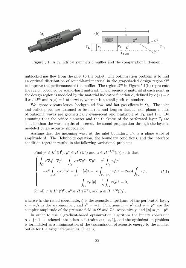
We consider a muffler consisting of an expansion chamber, an end inlet and, an endoutlet as shown in Figure 5.1(a). There may be a perforated pipe connecting theinlet and the outlet. The computational domain Ω = Ωl ∪ Ωu with Ωu = Ωd ∪ Ωp

is illustrated in Figure 5.1(b), which is an arbitrary cross-section through the centerof the cylindrical symmetric muffler 5.1(a). The non-overlapping regions Ωl and Ωu

separated by the interface ΓI. The non-design region Ωl is introduced to ensure

21

1

(a) Γs

ΓL ΓR

Γsym

Ωl

ΩdΩp

ΓI

r2r1

l

Ωm

1

(b)

Figure 5.1: A cylindrical symmetric muffler and the computational domain.

unblocked gas flow from the inlet to the outlet. The optimization problem is to findan optimal distribution of sound-hard material in the gray-shaded design region Ωd

to improve the performance of the muffler. The region Ωm in Figure 5.1(b) representsthe region occupied by sound-hard material. The presence of material at each point inthe design region is modeled by the material indicator function α, defined by α(x) = εif x ∈ Ωm and α(x) = 1 otherwise, where ε is a small positive number.

We ignore viscous losses, background flow, and hot gas effects in Ωa. The inletand outlet pipes are assumed to be narrow and long so that all non-planar modesof outgoing waves are geometrically evanescent and negligible at ΓL and ΓR. Byassuming that the orifice diameter and the thickness of the perforated layer ΓI aresmaller than the wavelengths of interest, the sound propagation through the layer ismodeled by an acoustic impedance.

Assume that the incoming wave at the inlet boundary, ΓL is a plane wave ofamplitude A. The Helmholtz equation, the boundary conditions, and the interfacecondition together results in the following variational problem:

Find pl ∈ H1(Ωl), pu ∈ H1(Ωu) and λ ∈ H−1/2(ΓI) such that

∫

Ωl

r∇ql · ∇pl +

∫

Ωu

αr∇qu · ∇pu − κ2

∫

Ωl

rqlpl

−κ2

∫

Ωu

αrqupu −∫

ΓI

rJqKλ+ iκ

∫

ΓL∪ΓR

rqlpl = 2iκA

∫

ΓL

rql,

∫

ΓI

rµJpK− i

κ

∫

ΓI

rζµλ = 0,

for all ql ∈ H1(Ωl), qu ∈ H1(Ωu), and µ ∈ H−1/2(ΓI),

(5.1)

where r is the radial coordinate, ζ is the acoustic impedance of the perforated layer,κ = ω/c is the wavenumber, and i2 = −1. Functions p = pl and p = pu are thecomplex amplitude of the pressure field in Ωl and Ωu, respectively, and JpK = pl− pu.

In order to use a gradient-based optimization algorithm the binary constraintα ∈ ε, 1 is relaxed into a box constraint α ∈ [ε, 1], and the optimization problemis formulated as a minimization of the transmission of acoustic energy to the muffleroutlet for the target frequencies. That is,

22

minα∈UJ (α;W, γ), (5.2)

where α ∈ U = β ∈ L∞(Ω) : 0 < ε ≤ β ≤ 1 a.e. in Ωd, β ≡ 1 ∈ Ω − Ωd is anew design variable, α = S(α) for filtering function S : L2(R2) → L2(R2), and W isthe set of all frequencies for which we are interested in to optimize the muffler. Theobjective function is defined by

J (α;W, γ) = Jp(S(α); γ) + Jt(S(α);W). (5.3)

Here, Jp is the penalty function and the primary objective function Jt is defined by

Jt(α;W) =∑

fj∈WJ(pl(α, fj)),

where for each fj ∈ W, pl(α, fj) ∈ H1(Ωl) is part of the triplet pl, pu, and λ thatsolves the state equation (5.1) for design α and wave number κ = 2πfj/c and

J(pl(α, fj)) =1

2|〈pl〉ΓR

|2,

where

〈pl〉ΓR =

∫ΓRrpl∫

ΓRr.

The finite element method is used to discretize problem (5.1). The material in-dicator function is assumed to be constant in each element. The optimization prob-lem (5.3) is solved numerically using the Method of Moving Asymptotes by adding thepenalty term to the objective function using a continuation approach for the penaltyparameter γ. Post-processing techniques are used in order to sharpen the edges of thesound-hard material. To compare the performance of the muffler designs, the trans-mission loss is used. The transmission loss of a muffler with the same cross-sectionalarea for the inlet and outlet is given by [44, 45]

TL = 10 log10

( |pi|2|po|2

),

where pi and po are the amplitudes of the incoming and outgoing acoustic pressure,respectively.

5.3 Selected numerical results

Two types of reactive mufflers are considered for the optimization, with and without aperforated pipe connecting the inlet and the outlet. We denote them by muffler withimpedance layer and muffler without impedance layer, respectively. The mufflers havethe same configuration; they have inlet and outlet pipes of radius r1 = 0.05 m, and

23

(a)

(b)

(c)

(d)

(e)

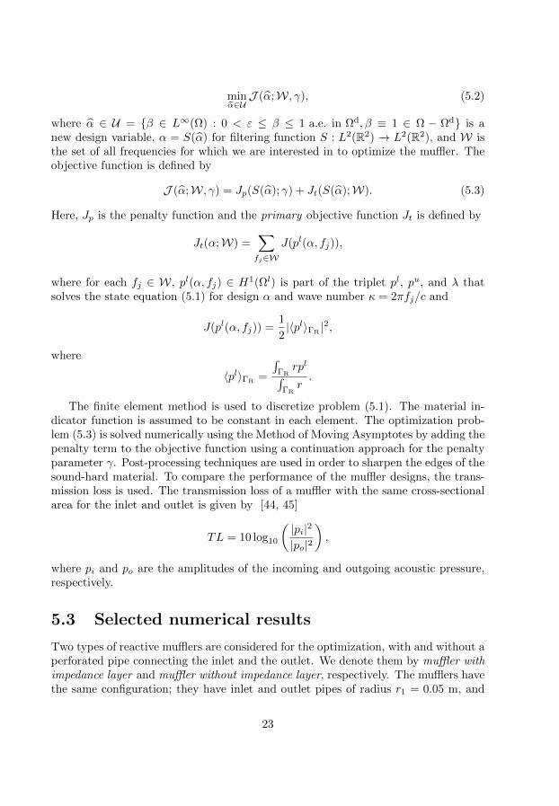
Figure 5.2: Final muffler designs from the continuation steps.(a) without penalty, (b) with penalty (γ = 1/2) and filter, (c)with penalty (γ = 500) and filter, (d) with penalty (γ = 500)and after filter is dropped, (e) after second level post-processing.

the expansion chamber has radius r2 = 0.1 m and length l = 0.5 m. The perforatedpipe of the muffler with impedance layer is characterized by a porosity of σ = 20%,thickness t = 1.5 mm, and orifice diameter d = 3.1 mm.

For all numerical experiments, we set ε = 10−8 as a lower bound for the designvariable αh. We use 28,672 square elements with side length 1.5625 mm for the finiteelement discretization. The number of design variables is 9,280. A plane wave ofamplitude A = 1 is injected into the muffler at the inlet boundary.

Figure 5.2 shows the designs from different steps of the continuation approach. Theoptimization is performed for a muffler without impedance layer at target frequencyf = 349 Hz. Figures 5.2(a), 5.2(b), and 5.2(c) are the designs obtained from theoptimization with γ = 0, γ = 1/2 and γ = 500, respectively. It shows that as theγ increases more and more the designs become more black and white. Figure 5.2(c)looks black and white except at the edges of the sound-hard material. To obtain asharp design, the filter is dropped and optimization is continued. Figure 5.2(d) showsthe sharpened design. In this experiment, we add the second phase of post-processing,in which the three narrow openings in Figure 5.2(d) are replaced by a single opening ofthe same total width and the optimization is continued one more round. Figure 5.2(e)shows the final design.

We optimize the two types of mufflers for single target frequency and multi-targetfrequencies. The single frequency optimization is performed for a frequency of 697 Hz.

24

0 200 400 600 800 1000 12000

10

20

30

40

Frequency (Hz)

Tra

nsm

issi

on L

oss

(dB

)

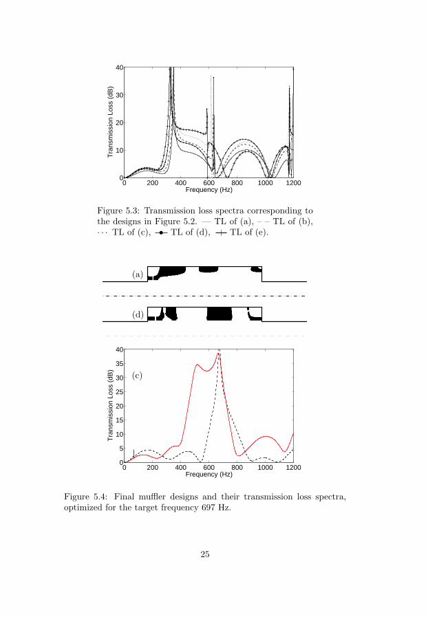
Figure 5.3: Transmission loss spectra corresponding tothe designs in Figure 5.2. — TL of (a), – – TL of (b),· · · TL of (c), • TL of (d), + TL of (e).

(a)

(d)

0 200 400 600 800 1000 12000

5

10

15

20

25

30

35

40

Frequency (Hz)

Tra

nsm

issi

on L

oss

(dB

)

(c)

Figure 5.4: Final muffler designs and their transmission loss spectra,optimized for the target frequency 697 Hz.

25

(a)

(b)

0 200 400 600 800 1000 12000

5

10

15

20

25

30

35

40

Frequency (Hz)

Tra

nsm

issi

on L

oss

(dB

)

(c)

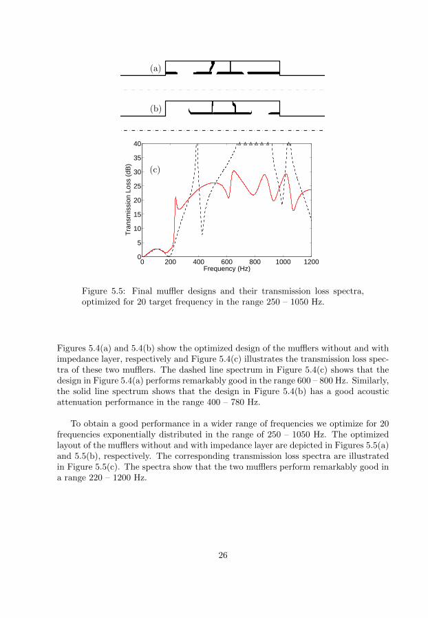
Figure 5.5: Final muffler designs and their transmission loss spectra,optimized for 20 target frequency in the range 250 – 1050 Hz.

Figures 5.4(a) and 5.4(b) show the optimized design of the mufflers without and withimpedance layer, respectively and Figure 5.4(c) illustrates the transmission loss spec-tra of these two mufflers. The dashed line spectrum in Figure 5.4(c) shows that thedesign in Figure 5.4(a) performs remarkably good in the range 600 – 800 Hz. Similarly,the solid line spectrum shows that the design in Figure 5.4(b) has a good acousticattenuation performance in the range 400 – 780 Hz.

To obtain a good performance in a wider range of frequencies we optimize for 20frequencies exponentially distributed in the range of 250 – 1050 Hz. The optimizedlayout of the mufflers without and with impedance layer are depicted in Figures 5.5(a)and 5.5(b), respectively. The corresponding transmission loss spectra are illustratedin Figure 5.5(c). The spectra show that the two mufflers perform remarkably good ina range 220 – 1200 Hz.

26

Bibliography

[1] A. E. Bryson Jr. Optimal control—1950 to 1985. Control Systems, IEEE,16(3):26–33, 1996.

[2] R. W. H. Sargent. Optimal control. Journal of Computational and AppliedMathematics, 124(1-2):361–371, 2000.

[3] J. T. Betts. Survey of numerical methods for trajectory optimization. Journalof Guidance, Control, and Dynamics, 21(2):193–207, 1998.

[4] A. E. Bryson Jr. and Y.C. Ho. Applied Optimal Control: Optimization, Es-timation, and Control. Halsted Press book. Hemisphere Publishing Company,1975.

[5] M. R. Hestenes. Calculus of variations and optimal control theory. Appliedmathematics series. R. E. Krieger Pub. Co., 1980.

[6] A. E. Bryson Jr. Applied Linear Optimal Control: Examples and Algorithms.Cambridge University Press, 2002.

[7] D. G. Hull. Optimal Control Theory for Applications. Mechanical EngineeringSeries. Springer, 2003.

[8] L. S. Pontryagin, V. G. Boltyanskii, R. V. Gamkrelidze, and E. F. Mishchenko.The mathematical theory of optimal processes. Wiley, 1962.

[9] D. Burghes and A. Graham. Control and Optimal Control: Theories with Appli-cations. Engineering science. Horwood Publishing Limited, 2004.

[10] D. E. Kirk. Optimal Control Theory: An Introduction. Dover books on engineer-ing. Dover Publications, Incorporated, 2004.

[11] O. von Stryk and R. Bulirsch. Direct and indirect methods for trajectory opti-mization. Annals of Operations Research, 37:357–373, 1992.

[12] A. V. Rao. A survey of numerical methods for optimal control. In 2009AAS/AIAA Astrodynamics Specialist Conference, pages 1–37, 2009.

27

[13] R. Bulirsch, E. Nerz, H. J. Pesch, and O. von Stryk. Combining direct andindirect methods in optimal control: Range maximization of a hang glider. InOptimal Control, volume 111 of International Series of Numerical Mathematics.Birkhuser, pages 273–288. Birkhauser Verlag, 1991.

[14] T. Binder, L. Blank, H. G. Bock, R. Bulirsch, W. Dahmen, M. Diehl, T. Kro-nseder, W. Marquardt, J. P. Schloder, and O. von Stryk. Introduction to modelbased optimization of chemical processes on moving horizons. In Online Op-timization of Large Scale Systems, pages 295–339. Springer Berlin Heidelberg,2001.

[15] E. Hairer, S. P. Nørsett, and G. Wanner. Solving Ordinary Differential EquationsI: Nonstiff problems. Springer series in computational mathematics. Springer-Verlag, 1991.

[16] J. C. Butcher. Numerical Methods for Ordinary Differential Equations. Wiley,2008.

[17] R. Pytlak. Numerical Methods for Optimal Control Problems with State Con-straints. Lecture Notes in Mathematics, 1707. Springer, 1999.

[18] S. Katsumata, S. Ichinose, T. Shoji, S. Nakaura, and M. Sampei. Throwingmotion control based on output zeroing utilizing 2-link underactuated arm. InProceedings of the 2009 conference on American Control Conference, pages 3057–3064, 2009.

[19] U. Mettin, A. S. Shiriaev, L. B. Freidovich, and M. Sampei. Optimal ball pitchingwith an underactuated model of a human arm. In IEEE International Conferenceon Robotics and Automation, ICRA 2010, pages 5009–5014, 2010.

[20] M. P. Bendsøe and N. Kikuchi. Generating optimal topologies in structural designusing a homogenization method. Computer Methods in Applied Mechanics andEngineering, 71(2):197–224, 1988.

[21] O. Sigmund. Tailoring materials with prescribed elastic properties. Mechanicsof Materials, 20(4):351–368, 1995.

[22] S. Zhou and Q. Li. Design of graded two-phase microstructures for tailoredelasticity gradients. Journal of Materials Science, 43:5157–5167, 2008.

[23] K. E. Jensen, P. Szabo, and F. Okkels. Topology optimization of viscoelasticrectifiers. Applied Physics Letters, 100(23):234102–234102–3, 2012.

[24] T. Borrvall and J. Petersson. Large-scale topology optimization in 3d usingparallel computing. Computer Methods in Applied Mechanics and Engineering,190(46-47):6201–6229, 2001.

28

[25] H. Guan, Y. J. Chen, Y. C. Loo, Y. M. Xie, and G. P. Steven. Bridge topologyoptimization with stress, displacement and frequency constraints. Computersand Structures, 81(3):131–145, 2003.

[26] L. Wang, P. K. Basu, and J. P. Leiva. Automobile body reinforcement by finiteelement optimization. Finite Elem. Anal. Des., 40(8):879–893, 2004.

[27] L. Krog, A. Tucker, M. Kemp, and R. Boyd. Topology optimization of aircraftwing box ribs. In 10th AIAA/ISSMO Multidisciplinary Analysis and Optimiza-tion Conference, page 16, 2004.

[28] O. Sigmund and J. Petersson. Numerical instabilities in topology optimization:A survey on procedures dealing with checkerboards, mesh-dependencies and localminima. Structural Optimization, 16:68–75, 1998.

[29] M. P. Bendsøe and O. Sigmund. Topology optimization. Theory, methods, andapplications. Springer, 2003.

[30] O. Sigmund. A 99 line topology optimization code written in matlab. Structuraland Multidisciplinary Optimization, 21(2):120–127, 2001.

[31] K. Svanberg. The method of moving asymptotes–a new method for struc-tural optimization. International Journal for Numerical Methods in Engineering,24(2):359–373, 1987.

[32] C. S. Jog and R. B. Haber. Stability of finite element models for distributed-parameter optimization and topology design. Computer Methods in Applied Me-chanics and Engineering, 130(34):203–226, 1996.

[33] T. Borrvall and J. Petersson. Topology optimization using regularized interme-diate density control. Computer Methods in Applied Mechanics and Engineering,190(37-38):4911–4928, 2001.

[34] M. P. Bendsøe. Optimal shape design as a material distribution problem. Struc-tural and Multidisciplinary Optimization, 1(4):193–202, 1989.

[35] A. Rietz. Sufficiency of a finite exponent in simp (power law) methods. Structuraland Multidisciplinary Optimization, 21(2):159–163, 2001.

[36] M. Stolpe and K. Svanberg. An alternative interpolation scheme for minimumcompliance topology optimization. Structural and Multidisciplinary Optimiza-tion, 22(2):116–124, 2001.

[37] A. Dıaz and O. Sigmund. Checkerboard patterns in layout optimization. Struc-tural optimization, 10:40–45, 1995.

[38] O. Sigmund. Morphology-based black and white filters for topology optimization.Structural and Multidisciplinary Optimization, 33(4-5):401–424, 2007.

29

[39] O. Sigmund. Design of Material Structures Using Topology Optimization. PhDthesis. Technical University of Denmark, 1994.

[40] T. E. Bruns and D. A. Tortorelli. Topology optimization of non-linear elasticstructures and compliant mechanisms. Computer Methods in Applied Mechanicsand Engineering, 190:3443–3459, 2001.

[41] B. Bourdin. Filters in topology optimization. International Journal for Numer-ical Methods in Engineering, 50(9):2143–2158, 2001.

[42] M. Y. Wang and S. Wang. Bilateral filtering for structural topology optimization.International Journal for Numerical Methods in Engineering, 63(13):1911–1938,2005.

[43] L. Munjal. Acoustics of ducts and mufflers with application to exhaust and ven-tilation system design. Wiley-Interscience publication. Wiley, 1987.

[44] T. W. Wu and G. C. Wan. Muffler performance studies using a direct mixed–bodyboundary element method and a three-point method for evaluating transmissionloss. Journal of Vibration and Acoustics, 118(3):479–484, 1996.

[45] D. D. Davis, G. M. Stokes, D. Moore, and G. L. Stevens. Theoretical andexperimental investigation of mufflers with comments on engine-exhaust mufflerdesign. NACA report 1192, 1954.

30