Embed Size (px)
Citation preview
Babes-Bolyai University Cluj-Napoca
Faculty of Mathematics and Computer Science
Livia-Mihaela Miholca(cas. Berchesan)
Contributions to the Theory of Equilibrium Problems
and Variational Inequalities
Ph.D. Thesis Summary
Scientific Advisor:
Prof. Univ. Dr. Kassay Gabor
Cluj-Napoca2014

Contents
Introduction 3
1 Preliminary notions and results 91.1 Convex sets, convex cones and intersection theorems . . . . . . . . . . . . . . . . . . . . . . . . . . . 91.2 Functions satisfying certain weakened convexity . . . . . . . . . . . . . . . . . . . . . . . . . . . . . 13
2 On Equilibrium Problems 162.1 Existence results for the scalar equilibrium problem . . . . . . . . . . . . . . . . . . . . . . . . . . . . 16
2.1.1 Existence results for equilibria on compact sets . . . . . . . . . . . . . . . . . . . . . . . . . . 172.1.2 Equilibria on noncompact sets . . . . . . . . . . . . . . . . . . . . . . . . . . . . . . . . . . . 20
2.2 Existence results for the vector equilibrium problem . . . . . . . . . . . . . . . . . . . . . . . . . . . 222.3 On vector equilibrium problems given by a sum of two functions . . . . . . . . . . . . . . . . . . . . 25
2.3.1 Existence results of (V EP ) . . . . . . . . . . . . . . . . . . . . . . . . . . . . . . . . . . . . . 272.3.2 The case of reflexive Banach spaces . . . . . . . . . . . . . . . . . . . . . . . . . . . . . . . . . 30
3 Existence results for variational inequalities 333.1 Generalized monotone and hemicontinuous operators . . . . . . . . . . . . . . . . . . . . . . . . . . . 333.2 Variational inequalities and generalized equations given by
properly quasimonotone operators . . . . . . . . . . . . . . . . . . . . . . . . . . . . . . . . . . . . . 373.3 A surjectivity result without monotonicity . . . . . . . . . . . . . . . . . . . . . . . . . . . . . . . . . 383.4 Results on variational inequalities and surjectivity given by
C and B-pseudomonotone operators . . . . . . . . . . . . . . . . . . . . . . . . . . . . . . . . . . . . . 393.5 On set-valued optimization problems and vector variational-like inequalities . . . . . . . . . . . . . . 39
3.5.1 Relationships between (SOP ) and W (SSV I) . . . . . . . . . . . . . . . . . . . . . . . . . . . 453.5.2 Relationships between (SOP ) and W (SMV I) . . . . . . . . . . . . . . . . . . . . . . . . . . 47
3.6 Vector variational-like inequalities . . . . . . . . . . . . . . . . . . . . . . . . . . . . . . . . . . . . . 50
Bibliography 57
2
Introduction
One of the most important topics in nonlinear analysis and several applied fields is the so called equilibrium problem.
The equilibrium theory, which is a part of the nonlinear analysis, provides a general, unified and natural framework
for the study of a large variety of problems, such as: optimization problems, variational inequalities problems,
saddle point problems, complementarity problems, Nash equilibria problems and fixed point problems. These pro-
blems often occur in economics, finance, network analysis, mechanics, physics, etc.
According to the bifunctions involved, one can distinguish two forms: the scalar equilibrium problem and the vector
equilibrium problem. In this thesis we deal with both forms.
The first equilibrium problem studied in the literature, was the scalar equilibrium problem which can be stated
as:
(SEP ) find a ∈ A such that f(a, b) ≥ 0 for all b ∈ B,
where A and B are two nonempty sets, and f : A×B → R is a given bifunction.
As far as we know the term ”equilibrium problem” was attributed in E. Blum and W. Oettli [22], but the problem
itself has been investigated more than twenty years before in a paper of Ky Fan [44] in connection with the so called
”intersection theorems” (i.e., results stating the nonemptiness of the intersection of a certain family of sets). Ky Fan
considered (SEP ) in the special case A = B a compact convex subset of a Hausdorff topological vector space and
termed it ”minimax inequality”. In the same year, H. Brezis, G. Nirenberg and G. Stampacchia [23] improved Ky
Fan’s result, extending it to a not necessarily compact set, but assuming instead a so-called ”coercivity condition”,
which is automatically satisfied when the set is compact.
(SEP ) has been extensively studied in recent years, see, for instance, M. Bianchi and R. Pini [18], M. Bianchi, G.
Kassay and R. Pini [20], M. Bianchi and S. Schaible [16], G. Bigi, M. Castellani and G. Kassay [21], W. Oettli [104],
A.N. Iusem, G. Kassay and W. Sosa [67], A.N. Iusem and W. Sosa [64].
New necessary (and in some cases also sufficient) conditions for existence of solutions in infinite dimensional
spaces were proposed, among others, in A.N. Iusem and W. Sosa [64], A.N. Iusem, G. Kassay and W. Sosa [67]
and G. Kassay and M. Miholca [78]. Note that A.N. Iusem, G. Kassay and W. Sosa [66] obtained existence results
concerning (SEP ) in finite dimensional cases, where, obviously the assumptions are less demanding.
The extension of the scalar equilibrium problem to vector equilibrium problems can be achieved in different
ways. Given a real topological vector space Y , a convex cone K ⊆ Y with intK 6= ∅ (where intK denotes the
interior of K), two nonempty sets A and B, and a bifunction f : A × B → Y , it can be formulated the following
vector equilibrium problem, known in the literature as the weak vector equilibrium problem:
(V EP ) find a ∈ A such that f(a, b) /∈ − intK for all b ∈ B.
(V EP ) has also been extensively studied in recent years, see, for instance, Q.H. Ansari, S. Schaible and J.C. Yao [8],
M. Bianchi, N. Hadjisavvas and S. Schaible [17], A. Capata and G. Kassay [30], D.T. Luc [93], and the references
therein.
3
The vector equilibrium problems contain as particular cases vector optimization problems, vector cone saddle
point problems, vector variational inequality problems, which arise in economics, physics, mechanics, etc. The latter
will be described in what follows.
Suppose that X is also a real topological vector space and denote by L(X,Y ) the set of all linear and continuous
maps from X to Y.
Let T : X → L(X,Y ), set A = B := domT.
(i) The Stampacchia vector variational inequality problem can be formulated as follows:
(SV V I) find a ∈ A such that 〈T (a), b− a〉 /∈ − intK for all b ∈ A.
If we consider f : A×A→ Y given by
f(a, b) = 〈T (a), b− a〉,
then (V EP ) is equivalent with (SV V I).
(ii) The Minty vector variational inequality problem can be formulated as follows:
(MV V I) find a ∈ A such that 〈T (b), b− a〉 /∈ − intK for all b ∈ A.
If we consider g : A×A→ Y given by
g(a, b) = f(b, a) = 〈T (b), a− b〉,
with f given at item (i), then one may see that (V EP ) with respect to g is equivalent with (MV V I).
Vector variational inequalities have shown to be important mathematical models in the study of many real
problems, in particular in network equilibrium models ranging from spatial price equilibrium problems and imperfect
competitive oligopolistic market equilibrium problems to general financial or traffic equilibrium problems.
In the setting of vector equilibrium problem, if we take Y := Rn, K ⊆ Rn a pointed convex cone, A = B
nonempty set, and f(a, b) = F (b) − F (a), where F : A → Rn, then the (V EP ) becomes the (finite dimensional)
vector optimization problem, denoted (V OP ). For a presentation and results concerning (V OP ) the reader can
consult, for instance, the monograph of N. Popovici [109] and the references therein.
In 1998, Giannessi [54] first used the so called Minty-type vector variational inequality to establish the necessary
and sufficient conditions for a point to be an efficient solution of a vector optimization problem for differentiable
and convex functions. Since then, several researchers have studied (V OP ) by using several kinds of Minty-type
vector variational inequality under different assumptions, see S. Al-Homidan and Q.H. Ansari [1], Q.H. Ansari and
G.M. Lee [3], Q.H. Ansari, M. Rezaie and J. Zafarani [5], Q.H. Ansari and J.-K. Yao [6], G.R. Garzon, R.O. Gomez
and A.R. Lizana [53], S.K. Mishra and S.Y. Wang [101] and the references therein. Consequently, vector variational
inequalities have been generalized in various directions, in particular, vector variational-like inequality problems,
see S. Al-Homidan and Q.H. Ansari [1], F. Giannessi, A. Maugeri and P.M. Pardalos [56], T. Jabarootian and J.
Zafarani [69], S.K. Mishra and S.Y. Wang [101], M. Rezaie and J. Zafarani [110], X.M. Yang and X.Q. Yang [122]
and the references therein.
The aim of this thesis is to extend some of the known existence results and to present new results for (SEP ),
(V EP ), and for different kinds of variational inequalities.
The thesis consists on three chapters.
4
The mathematical notions and results needed for the study of scalar and vector equilibrium problems are recalled
in Chapter 1. Section 1.1 contains properties concerning cones, convex sets, separation and intersection theorems in
infinite dimensional spaces, different generalizations of the upper semicontinuity from the scalar case and classical
monotonicity for operators. Then, in Section 1.2, there are presented weakened convexity notions for vector-valued
functions and their characterizations.
Chapter 2 is devoted to some existence results for (SEP ) and (V EP ). More specifically, Section 2.1 deals
with (SEP ) in the case of compact or noncompact sets. In Subsection 2.1.1, using pseudo-upper semicontinuity
instead of upper semicontinuity, we extend the existence result of G. Kassay and J. Kolumban [77]. In Subsection
2.1.2, in the case of noncompact sets, we are able to obtain existence results for (SEP ) in infinite dimensional
case, without monotonicity by strengthening the continuity assumption on f with respect to the first variable. The
absence of compactness of the set A can be overcome by considering different types of so-called coercivity conditions.
In Section 2.2 we deal with (V EP ) and under K-pseudo upper semicontinuity we extend a result of A. Capata
and G. Kassay [30].
In the last section of this chapter, Section 2.3, we obtain existence results for a special case of (V EP ) when
f(x, y) = g(x, y)+h(x, y). This problem, with g, h : A×A→ R, captured less attention, although it was investigated
already in E. Blum and W. Oettli [22], where the authors obtained existence results by imposing their assumptions
separately on g and h. As stressed in [22], if g = 0, the result becomes a variant of Ky Fan’s theorem [46], whereas
for h = 0 it becomes a variant of the Browder-Minty theorem for variational inequalities (see F.E. Browder [25], [26],
G.J. Minty [100]). Also, in this section the special case of reflexive Banach spaces endowed with the weak topology
is separately treated; in that case mild sufficient conditions for guaranteeing coercivity are presented.
In Chapter 3 we study different kinds of variational inequalities. Section 3.1 is devoted to the study of generalized
monotone operators. The original concept of monotonicity has been extended in various directions. Apart from their
theoretical interest, generalized monotone operators are often more suitable to describe problems than the original
concept of monotonicity, in disciplines such as economics, management science, probability theory and other applied
sciences. Results concerning surjectivity are therefore especially important, as they guarantee, in particular, the
existence of zeros of these operators.
In Section 3.2 sufficient conditions for the solvability of variational inequalities in infinite dimensional case,
given by properly quasimonotone and quasicoercive operators, are provided. In the special case when the domain
of the operator is the whole space, it shows the existence of zeroes for such kind of operators. The surjectivity
results from Section 3.3 are obtained without monotonicity but with a stronger continuity condition. In Section
3.4 we deal with C-pseudomonotone operators and we establish a result concerning variational inequalities given by
C-pseudomonotone operators, which can be seen in the framework of a reflexive Banach space a generalization of a
similar result by D. Inoan and J. Kolumban [63].
Section 3.5 is devoted to the study of (Minty and Stampacchia) generalized variational-like inequalities with set-
valued mappings in topological spaces, which include as a special case the strong vector variational-like inequalities.
Motivated by the works of T.Q. Bao, B.S. Mordukhovich [13], Y.P. Fang, N.J. Huang [47], Y.P. Fang, N.J. Huang
[48], A.P. Farajzadeh, A.A. Harandi, K.R. Kazmi [49] and J. Zeng, S.J. Li [129], in this section we introduce
several kinds of generalized invexity for set-valued mappings and study the relationships among them. Then, we
establish solution relationships between several kind of vector variational-like inequality problems and a set-valued
optimization problem by means of weak contingent generalized subdifferential defined for set-valued mappings.
In Section 3.6 we study the Minty vector variational-like inequality and (weak) Stampacchia vector variational-
like inequality (which are closely related to the concepts of invex and preinvex functions which generalize the notion
5
of convexity of functions), defined by means of Mordukhovich limiting subdifferentials in Asplund spaces. The
concept of invexity was first introduced by M.A. Hanson [60]. More recently, the characterization and applications
for generalized invexity were studied by many authors, see Q.H. Ansari and J.-K. Yao [6], A. Cambini and L.
Martein [29], A. Chinchuluun and P.M. Pardalos [37], T. Jabarootian and J. Zafarani [69], G.R. Garzon, R.O.
Gomez and A.R. Lizana [52], M. Soleimani-damaneh [116], M. Soleimani-damaneh [117], X.M. Yang, X.Q. Yang
and K.L. Teo [123], X.M. Yang, X.Q. Yang and K.L. Teo [126] and the references therein.
We obtain some relationships between a solution of (V OP ) and these vector variational-inequalities using the
concept of generalized invexity for vector valued functions. The main results in S. Al-Homidan and Q.H. Ansari [1],
Q.H. Ansari, M. Rezaie and J. Zafarani [5], M. Rezaie and J. Zafarani [110] were obtained in the setting of Clarke
subdifferential. Since the class of Clarke subdifferential is larger than the class of Mordukhovich subdifferential
(see B. Mordukhovich [102]), some authors studied the vector variational-like inequalities and vector optimization
problems in the setting of Mordukhovich subdifferential in order to obtain stronger results. By means of several
examples we show that our results are stronger than the similar statements in the literature.
The author’s original contributions are the following:
Chapter 2: Definition 2.1.1, Lemma 2.1.2, Example 2.1.4, Theorem 2.1.5, Theorem 2.1.11, Theorem 2.1.17,
Theorem 2.1.18, Lemma 2.2.3, Definition 2.2.4, Definition 2.2.5, Definition 2.2.6, Theorem 2.2.7, Theorem 2.2.10,
Theorem 2.2.11, Theorem 2.2.14, Lemma 2.3.16, Definition 2.3.20, Proposition 2.3.21, Example 2.3.22, Lemma
2.3.23, Lemma 2.3.24, Lemma 2.3.25, Example 3.6.19, Theorem 2.3.28, Example 2.3.31, Theorem 2.3.33, Proposi-
tion 2.3.34, Remark 2.3.35, Lemma 2.3.36, Lemma 2.3.38, Proposition 2.3.39, Lemma 2.3.40, Theorem 2.3.41 and
Corollary 2.3.42.
Chapter 3: Definition 3.1.5, Remark 3.1.6, Lemma 3.1.14, Theorem 3.2.1, Example 3.2.4, Definition 3.3.1, Re-
mark 3.3.2, Example 3.3.3, Theorem 3.3.4, Corollary 3.3.5, Example 3.3.6, Theorem 3.4.1, Theorem 3.4.2, Definition
3.5.7, Definition 3.5.13, Proposition 3.5.14, Example 3.5.15, Example 3.5.16, Definition 3.5.20, Definition 3.5.21,
Theorem 3.5.22, Example 3.5.23, Theorem 3.5.31, Theorem 3.5.32, Corollary 3.5.33, Corollary 3.5.34, Corollary
3.5.35, Theorem 3.5.36, Corollary 3.5.37, Theorem 3.5.38, Corollary 3.5.39, Corollary 3.5.40, Corollary 3.5.41, The-
orem 3.5.42, Corollary 3.5.43, Corollary 3.5.44, Corollary 3.5.45, Theorem 3.5.46, Corollary 3.5.47, Theorem 3.5.48,
Corollary 3.5.49, Corollary 3.5.50, Corollary 3.5.51, Theorem 3.5.52, Corollary 3.5.53, Example 3.6.9, Definition
3.6.10, Definition 3.6.13, Theorem 3.6.16, Theorem 3.6.17, Example 3.6.19, Theorem 3.6.21, Corollary 3.6.22, Ex-
ample 3.6.24, Theorem 3.6.25, Corollary 3.6.26, Theorem 3.6.27 and Example 3.6.29.
The author’s results included in this thesis are published in:
1. M. Miholca, Vector variational-like inequalities and set-valued optimization problems, Ann. of Tiberiu
Popoviciu Seminar 10 (2012), 75-85.
2. G. Kassay, M. Miholca, Existence results for variational inequalities with surjectivity consequences related
to generalized monotone operators, J. Optim. Theory Appl. 159 (2013), 721-740.
3. M. Miholca, On set-valued optimization problems and vector variational-inequalities, Optim. Lett. 8(2)
(2014), 463-476.
4. M. Miholca, Vector variational-like inequalities and vector optimization problems, Carpathian J. Math.
30(1) (2014), 101-108
or in publication process:
5. G. Kassay, M. Miholca, On vector equilibrium problems given by a sum of two functions, submitted.
6. M. Miholca, Lipschitz B-preinvex functions in Asplund spaces, submitted.
7. M. Miholca, On vector variational-like inequalities and vector optimization problems in Asplund spaces,
6
accepted for publication in Studia Mathematica Universitatis Babes-Bolyai,
while some of them are completely new in the sense that they appear for the first time here.
A significant part of the original results proved in this thesis were also presented at the following scientific
conferences:
• 10th International Symposium on Generalized Convexity and Monotonicity (GCM10), August 22-27, 2011,
Cluj-Napoca, Romania.
• 11th EUROPT Workshop on Advances in Continuous Optimization, June 26-28, 2013, Firenze, Italy.
• The Fourth International Conference on Continuous Optimization (ICCOPT), July 27-August 1, 2013, Lisbon,
Portugal.
• Conference on Numerical Analysis and Optimization (NAOiii), January 5-9, 2014, Mascat, Oman.
Keywords: scalar equilibrium problem, vector equilibrium problem, variational inequalities, vector variational-
like inequalities, generalized equations, set-valued optimization problem, vector optimization problem, minimax i-
nequality, Banach space, Asplund space, coercivity conditions, generalized monotone operators, F−hemicontinuous
operator, properly quasimonotone operator, C and B−pseudomonotone operators, KKM−operator, properly quasi-
monotone function,, essentially quasimonotone function, quasiconvex function, prequasi-invex function, K−convex-
like function, weakly quasi-invex function, K−concave function, K−pseudo-upper semicontinuous function,
(K,L)−weakly-quasi-invex function.
7
Acknowledgements
My first gratitude goes to my supervisor Prof. Univ. Dr. Gabor Kassay to whom I am deeply indebted for his
constant support, continuous supervision, fruitful discussions, invaluable hints and assistance during my doctoral
study. It has a privilege to be a member of his CNCS-UEFISCDI Project, cod PN-II-ID-PCE-2011-3-0024.
Special thanks go to my guidance committee: Conf. Univ. Dr. Nicolae Popovici, Conf. Univ. Dr. Cornel
Pintea and Prof. Univ. Dr. Csaba Varga for the continuous supervision and fruitful discussions.
I also want to thank all the professors from the Analysis and Optimization Research Group, Department of
Mathematics, Babes-Bolyai University.
I am also grateful to the Faculty of Mathematics and Computer Science, Cluj-Napoca, for providing me a nice
research environment.
Sincere thanks goes to my family, my parents, my husband and my child Darius for love, support, patience,
understanding and encouragements.
8
Chapter 1
Preliminary notions and results
In this thesis, we use the well-known notions of vector space, topological space, and topological vector space. All
vector spaces are real. Basic definitions and properties concerning these and other spaces can be found, for instance,
in the books by I. Muntean [103], H.L. Royden [112], W. Rudin [114], J. Schauder [115], J. Von Neumann [119] and
K. Yosida [127].
If X and Y are topological vector spaces, we denote by
L(X,Y ) := {ξ : X → Y | ξ linear and continuous},
and by 〈·, ·〉 : L(X,Y )×X → Y we understand
〈ξ, x〉 = ξ(x), ∀ξ ∈ L(X,Y ), ∀x ∈ X.
In the particular case when Y := R, L(X,Y ) := X∗ (the dual of X) and 〈·, ·〉 : X∗ ×X → R is the duality pairing
given by
〈x∗, x〉 = x∗(x), ∀x∗ ∈ X∗, ∀x ∈ X.
Let {xα}α ⊆ X be a net and x ∈ X. Recall that xα converges weakly to x (denoted xα ⇀ x) iff for each x∗ ∈ X∗
one has 〈x∗, xα〉 converges (in R) to 〈x∗, x〉. Recall also that in a reflexive Banach space, every closed, convex and
bounded subset is weakly compact.
1.1 Convex sets, convex cones and intersection theorems
Definition 1.1.1. A subset A of a vector space X is called convex iff
λA+ (1− λ)A ⊆ A for all λ ∈ [0, 1].
For a subset A of a topological vector space X, we denote by intA, clA,
coA, riA, the interior, the closure, the convex hull, and the relative interior of A, respectively.
We recall here that a cluster point of a set A in a topological space is a point a whose neighborhoods all contain at
least one point of the set A other than a. By A′
we denote the set of cluster points of A.
Definition 1.1.2. Let X be a vector space. A subset K ⊆ X is said to be a cone iff it is nonempty and λK ⊆ Kfor each λ ≥ 0. A cone K ⊆ X is said to be convex iff it is a convex set.
9
A cone K in a vector space is convex if and only if K +K ⊆ K. For more details, see R. Hartley [61].
Definition 1.1.3. A cone in a vector space is said to be:
(i) nontrivial iff K 6= {0};
(ii) proper iff K 6= X;
(iii) pointed iff K ∩ (−K) = {0};
(iv) solid iff intK 6= ∅.
Given a convex cone K of a topological vector space X, the dual cone of K is defined by
K∗ := {x∗ ∈ X∗ | x∗(k) ≥ 0 for all k ∈ K}.
Often, as in the case of real numbers, we need an order relation on vector spaces. This relation will be defined
below. Given a pointed convex cone K in a vector space X, the relation ≤K is defined as follows
y ≤K x iff x− y ∈ K.
For arbitrary x, y, z, t, the following properties are satisfied:
(i) x ≤K x;
(ii) x ≤K y and z ≤K t implies x+ z ≤K y + t;
(iii) x ≤K y and y ≤K x implies x = y;
(iv) x ≤K y and λ ∈ R+ implies λx ≤K λy.
The relation above is in particular a partial order.
Lemma 1.1.4. (see, for instance, A. Capata and G. Kassay [30]) Let K be a nontrivial solid convex cone of a
topological vector space X. If k∗ ∈ K∗ is a nonzero functional, then k∗(k) > 0 for all k ∈ intK.
If X denotes a normed space or a Banach space and K is a closed convex set in X, we denote by PK(y) the
projection of y onto K, that is PK(y) ∈ K and
‖y − PK(y)‖ = d(y,K) := infz∈K‖z − y‖.
The next result is a variant of the celebrated Hahn-Banach theorem. Known as the separation of convex sets by
closed hyperplanes, it is a cornerstone property of nonlinear and convex analysis.
Theorem 1.1.5. [41] Let X be a topological vector space, and let A and B be nonempty convex subsets of X
satisfying the following conditions:
(i) B has a nonempty interior;
(ii) A ∩ (intB) = ∅.
Then there exist x∗ ∈ X∗, x∗ 6= 0, and r ∈ R such that x∗(a) ≤ r ≤ x∗(b) whenever a ∈ A and b ∈ B.
10
If X is a topological vector space, A and B are nonempty subsets of X, we say that A and B can be strongly
separated iff there exists x∗ ∈ X∗, x∗ 6= 0 such that
infa∈A〈x∗, a〉 > sup
b∈B〈x∗, b〉.
Remark 1.1.6. Assumption (i) is essential in Theorem 1.1.5 even in case A ∩ B = ∅, provided X is infinite
dimensional, as the example below shows.
Example 1.1.7. Let X be an infinite dimensional topological vector space and let x∗ : X → R be a discontinuous
linear functional. Set
C = {x ∈ X | x∗(x) = 0} and D = {x ∈ X | x∗(x) = 1}.
We can observe that these sets are convex (in fact affine) and dense in X, intC = intD = ∅, C ∩D = ∅ and cannot
be separated by a closed hyperplane.
Remark 1.1.8. In finite dimensional spaces, any nonempty convex set has nonempty relative interior (see [111])
and Theorem 1.1.5 holds without (i) and a weaker condition (ii).
Theorem 1.1.9. [111] Let A and B be nonempty convex sets in Rn such that riA ∩ riB = ∅. Then there exists a
hyperplane separating A and B properly, that is there exists some y ∈ Rn satisfying:
infa∈A〈y, a〉 ≥ sup
b∈B〈y, b〉
and
〈y, a1〉 > 〈y, b1〉,
for some a1 ∈ A and b1 ∈ B.
Let X be a vector space and F : X → [−∞,+∞] be a function. The effective domain, level sets, and epigraph
of F are defined by
domF := {x ∈ X | F (x) <∞},L(F, r) := {x ∈ X | F (x) ≤ r}, r ∈ R,epiF := {(x, r) ∈ X × R | F (x) ≤ r},
respectively.
Definition 1.1.10. (see, for instance, [15], [111]) Let X be a topological space and F : X → [−∞,+∞] be a
function.
(i) F is said to be lower semicontinuous at a point x0 ∈ X iff for any ε > 0 there exists a neighbourhood U of
x0 such that f(x0) < f(x) + ε for all x ∈ U.
(ii) F is said to be upper semicontinuous at a point x0 ∈ X iff for any ε > 0 there exists a neighbourhood U of
x0 such that f(x)− ε < f(x0) for all x ∈ U.
In the case of normed spaces, F is lower semicontinuous at a point x0 ∈ X iff for any sequence {xn}n ⊆ X,
xn → x0 ⇒ F (x0) ≤ lim infn→∞
F (xn)
and it is upper semicontinuous at a point x0 ∈ X iff for any sequence {xn}n ⊆ X,
xn → x0 ⇒ lim supn→∞
F (xn) ≤ F (x0).
11
Theorem 1.1.11. (see, for instance, [15], [111]) Let X be a Hausdorff topological vector space and
F : X → [−∞,+∞] be a function. Then the following assertions are equivalent:
(i) F is lower semicontinuous, i.e., F is lower semicontinuous at every point in X;
(ii) epiF is closed in X × R;
(iii) for every r ∈ R, L(F, r) is closed in X.
Definition 1.1.12. Let X be a normed space and F : X → [−∞,+∞] be a function. F is said to be upper
hemicontinuous iff it is upper semicontinuous on any segment contained on X.
Let T : X → 2Y be a set-valued map and K ⊆ Y a pointed convex cone. The domain, graph and epigraph of T
are defined by
domT := {x ∈ X | T (x) 6= ∅},gphT := {(x, y) ∈ ×Y | x ∈ domT, y ∈ T (x)},
epiT := {(x, y) ∈ X × Y | x ∈ domT, y ∈ T (x) +K},
respectively.
The next concept turned to be very important in the last fifty years.
Definition 1.1.13. (see, for instance, [25]) Let T : X → 2X∗
be a set-valued map. We say that T is monotone iff
for every x1, x2 ∈ domT, y1 ∈ T (x1),
y2 ∈ T (x2) one has
〈y2 − y1, x2 − x1〉 ≥ 0.
The classical concept of monotonicity has been extended in several ways. Among them we mention the following
two.
Definition 1.1.14. (see, for instance, [58]) Let T : X → 2X∗
be a set-valued map. We say that T is pseudomonotone
iff for every x1, x2 ∈ domT,
y1 ∈ T (x1), y2 ∈ T (x2) one has
〈y1, x2 − x1〉 ≥ 0⇒ 〈y2, x2 − x1〉 ≥ 0.
Definition 1.1.15. (see, for instance, [58]) Let T : X → 2X∗
be a set-valued map. We say that T is quasimonotone
iff for every x1, x2 ∈ domT,
y1 ∈ T (x1), y2 ∈ T (x2) one has
〈y1, x2 − x1〉 > 0⇒ 〈y2, x2 − x1〉 ≥ 0.
In what follows, in this section, we suppose that A is a nonempty subset of a topological vector space X and
T : X → 2X is a set-valued map with domT = A.
Definition 1.1.16. T is said to be a KKM-mapping iff, for every finite subset {a1, a2, ..., an} of A, the following
inclusion holds:
co{a1, a2, ..., an} ⊆n⋃i=1
T (ai).
The next celebrated lemma was given by B. Knaster, C. Kuratowski and S. Mazurkiewicz [83] in finite dimen-
sional spaces, while in infinite dimensional spaces it was established by Ky Fan [44].
Lemma 1.1.17. [44] Let T : A→ 2X be a KKM-mapping satisfying the following conditions:
(i) T (a) is closed for all a ∈ A;
12
(ii) there exists a ∈ A such that T (a) is a compact set.
Then⋂a∈A T (a) 6= ∅.
To establish our results in Section 3.4 below we use the following important intersection theorem due to H.
Brezis, G. Nirenberg and G. Stampacchia [23] which extended the above intersection theorem of Ky Fan [44].
Theorem 1.1.18. [23]. Let T : A→ 2X be KKM mapping such that:
(i) clT (y0) is compact for some y0 ∈ A;
(ii) For each y ∈ A and for each finite dimensional subspace Z of X, T (y) ∩ Z is closed;
(iii) For each line segment D of X :
cl( ∩y∈A∩D
T (y)) ∩D = ( ∩y∈A∩D
T (y)) ∩D.
Then ∩y∈A
T (y) 6= ∅.
Remark 1.1.19. If A is convex, closed and T (y) ⊆ A for every y ∈ A, then the hypothesis (iii) can be replaced by
(iii′) for every line segment D of X
cl( ∩y∈D
T (y)) ∩D = ( ∩y∈D
T (y)) ∩D.
1.2 Functions satisfying certain weakened convexity
Let X be a vector space and A a nonempty subset of it.
Definition 1.2.1. (see, for instance, [58]) If A ⊆ X is convex, a function F : A→ R is called quasiconvex iff for all
x, y ∈ A and for each λ ∈ [0, 1] the following inequality holds:
F (λx+ (1− λ)y) ≤ max{F (x), F (y)}.
Definition 1.2.2. (see, for instance, [58]) If A ⊆ X is convex, a function F : A → R is called semistrictly
quasiconvex iff for all x, y ∈ A the following implication holds:
F (x) < F (y)⇒ ∀λ ∈ (0, 1), F (λx+ (1− λ)y) < F (y).
If F is semistrictly quasiconvex and lower semicontinuous, then it is quasiconvex. For more details, see N.
Hadjisavvas [58], I. Konnov [87] and I. Konnov, D.T. Luc and A.M. Rubinov [89].
Definition 1.2.3. (see, for instance, [58]) If A ⊆ X is convex, a function F : A→ R is called pseudo-convex iff for
all x, y ∈ K and for each λ ∈ (0, 1) the following implication holds:
F (αx+ (1− α)y) ≥ F (x)⇒ F (αx+ (1− α)y) ≤ F (y).
The next concept was introduced by Ky Fan [43] in order to extend some minimax results.
13
Definition 1.2.4. [43] Let B be a nonempty set. A bifunction f : A×B → R is said to be Ky Fan concave-convex
iff for all a1, a2 ∈ A and all λ ∈ [0, 1] there exists a ∈ A such that
f(a, b) ≥ λf(a1, b) + (1− λ)f(a2, b) for all b ∈ B,
and for all b1, b2 ∈ B and all µ ∈ [0, 1] there exists b ∈ B such that
f(a, b) ≤ µf(a, b1) + (1− µ)f(a, b2) for all a ∈ A.
Some years later, H. Konig [86] extended the above notion of Ky Fan in order to generalize his minimax result.
Definition 1.2.5. [86] Let B be a nonempty set. A bifunction f : A×B → R is said to be Konig concave-convex
iff for all a1, a2 ∈ A there exists a ∈ A such that
f(a, b) ≥ 1
2[f(a1, b) + f(a2, b)] for all b ∈ B,
and for all b1, b2 ∈ B there exists b ∈ B such that
f(a, b) ≤ 1
2[f(a, b1) + f(a, b2)] for all a ∈ A.
The convexity concept for scalar functions has been extended in a natural way for vector-valued functions,
according to the partial order introduced by the cone K.
Definition 1.2.6. Let X and Y be vector spaces, let A be a nonempty subset of X, and let K ⊆ Y be a convex
cone. A function F : A→ Y is said to be:
(i) K-convex iff A is convex and, for all a1, a2 ∈ A and all λ ∈ [0, 1], the following inequality holds:
F (λa1 + (1− λ)a2) ≤K λF (a1) + (1− λ)F (a2);
F is said to be K-concave iff −F is K-convex.
(ii) K-convexlike iff, for all a1, a2 ∈ A and all λ ∈ [0, 1], there exists a ∈ A such that
F (a) ≤K λF (a1) + (1− λ)F (a2);
(iii) K-subconvexlike iff there exists k ∈ intK such that, for all a1, a2 ∈ A, λ ∈ [0, 1] and all ε > 0, there exists
a ∈ A satisfying the following inequality:
F (a) ≤K λF (a1) + (1− λ)F (a2) + εk.
Definition 1.2.6 (i) can be found in B. D. Craven [38], (ii) is due to Ky Fan [43], while (iii) originates from V.
Jeyakumar [71]. Obviously, when intK 6= ∅, then the K-convexlikeness of F implies the K-subconvexlikeness of F .
Next we present some monotonicity conditions for scalar bifunctions considered within the literature in the recent
years. Most of these notions were inspired by similar (generalized) monotonicity concepts defined for operators acting
from a topological vector space to its dual space.
Let A ⊆ X be a convex set.
Definition 1.2.7. (see, for instance, [18]) The bifunction f : A×A→ R is said to be
14
(i) monotone iff f(x, y) + f(y, x) ≤ 0 for all x, y ∈ A;
(ii) quasimonotone iff the following implication holds:
f(x, y) > 0⇒ f(y, x) ≤ 0;
(iii) properly quasimonotone iff for all x1, · · · , xn ∈ A and all λ1, · · · , λn ≥ 0 such that∑ni=1 λi = 1 it holds that
min1≤i≤n
f(xi,
n∑j=1
λjxj) ≤ 0.
Proper quasimonotonicity was introduced by Zhou and Chen in [130] under the name of 0− diagonal quasicon-
cavity (see also [18]).
In the case of variational inequalities, proper quasimonotonicity is stronger than quasimonotonicity, as defined,
e.g., in S. Karamardian and S. Schaible [74]. In the general case it neither implies quasimonotonicity nor is implied
by it, see M. Bianchi and R. Pini [18].
The result below, known as ”Ky Fan’s” minimax inequality theorem, plays a crucial role within nonlinear and
convex anaysis and it is an easy consequence of Lemma 1.1.17.
Theorem 1.2.8. [46]. Let A be a compact convex set in a Hausdorff topological vector space. If f : A × A → Ris such that for every x ∈ A, f(x, ·) is quasiconvex and for every y ∈ A, f(·, y) is upper semicontinuous, then there
exists x ∈ A such that
f(x, y) ≥ infx∈A
f(x, x) for all y ∈ A.
15
Chapter 2
On Equilibrium Problems
One of the most important topics in nonlinear analysis (see, for instance, P.M. Pardalos, T.M. Rassias and A.A.
Khan [107]) and several applied fields is the so called equilibrium problem. According to the bifunctions involved,
one can distinguish two forms: the scalar equilibrium problem and the vector equilibrium problem. In this chapter
we deal with both forms.
The equilibrium problem has been extensively studied in recent years (see, for instance, M. Bianchi, G. Kassay and
R. Pini [20], O. Chadli, Y. Chiang and S. Huang [31], X.H. Gong [57], A.N. Iussem and W. Sossa [65], P. Kas, G.
Kassay and Z. Boratas-Sensoy [75], G. Kassay [76], I.V. Konnov and J.C. Yao [88]). One of the reasons is that
it has among its particular cases, optimization problems, saddlepoint (minimax) problems (see, for instance, [42],
F. Ferro [50], S. Paeck [106]), variational inequalities (monotone or otherwise) (see, for instance, L.B. Batista
Dos Santos, G. Ruiz-Garzon and M.A. Rojas-Medar [14], S.S. Chang and Y. Zhang [32], G.-Y. Chen and Q.M.
Cheng [33], B. Chen and N.J. Huang [34], C. Finet, L. Quarta and C. Troestler [51], F. Giannessi [54], K.L. Lin,
D.P. Yang and J.C. Yao [91]), Nash equilibrium problems, and other problems of interest in many applications (see,
J.P. Aubin [10], T. Basar and G. J. Olsder [12], A.J. Jones [72], H.W. Kuhn [90], N.N. Vorob’ev [120] or E. Blum
and W. Oettli [22] for a survey).
2.1 Existence results for the scalar equilibrium problem
Throughout this section we suppose that A is a nonempty subset of a topological space X and B is a nonempty
set.
Let f : A×B → R be a given bifunction. The scalar equilibrium problem consists on:
(SEP ) finding an element a ∈ A such that f(a, b) ≥ 0 for all b ∈ B.
(SEP ) has been extensively studied in recent years, see, for instance, M. Bianchi and R. Pini [18], [19], M.
Bianchi and S. Schaible [16], G. Bigi, M. Castellani and G. Kassay [21], E. Blum and W. Oettli [22], A.N. Iusem, G.
Kassay and W. Sosa [67], A.N. Iusem and W. Sosa [64]. As we have already mentioned in the Introduction, the term
”equilibrium problem” was attributed in E. Blum and W. Oettli [22], but the problem itself has been investigated
more than twenty years before in a paper of Ky Fan [44] in connection with the so called ”intersection theorems”
(i.e., results stating the nonemptiness of a certain family of sets). Ky Fan considered (SEP ) in the special case
A = B a compact convex subset of a Hausdorff topological vector space and termed it ”minimax inequality”. In
the same year, H. Brezis, G. Nirenberg and G. Stampacchia [23] improved Ky Fan’s result, extending it to a not
16
necessarily compact set, but assuming instead a so-called ”coercivity condition”, which is automatically satisfied
when the set is compact.
Recent results on (SEP ) emphasizing existence of solutions can be found in M. Bianchi and R. Pini [18], [19],
M. Bianchi and S. Schaible [16], [70], W. Oettli [104], and many other papers. New necessary (and in some cases
also sufficient) conditions for existence of solutions in infinite dimensional spaces were proposed, among others, by
A.N. Iusem and W. Sosa [64], A.N. Iusem, G. Kassay and W. Sosa [67] and G. Kassay and M. Miholca [78].
Looking on the proofs given for existence results, one may detect two fundamental methods: fixed point methods
(intersection theorems mostly based on Brouwer’s fixed point theorem), and separation methods (Hahn-Banach type
theorems).
In what follows we divide our study on (SEP ) according to the nature of the set A, namely when this set is
compact and when is not.
2.1.1 Existence results for equilibria on compact sets
In this subsection we introduce a definition for scalar functions which is weaker than that of upper semicontinuity.
Definition 2.1.1. A function F : A→ R is said to be pseudo-upper semicontinuous at a ∈ A iff F (a) < 0 implies
that there exist c > 0 and a neighbourhood U of a such that F (x) + c < 0 for all x ∈ A ∩ U.F is said to be pseudo-upper semicontinuous on A iff it is pseudo-upper semicontinuous at a ∈ A for all a ∈ A.
The pseudo-upper semicontinuity of a function can be characterized as follows. Let V(a) be the set of all
neighbourhoods of a.
We have the following characterization which, as far as we know, is new in the literature.
Lemma 2.1.2. F is pseudo-upper semicontinuous at a ∈ A ∩A′ if and only if
F (a) < 0 =⇒ lim supx→a
F (x) < 0.
Remark 2.1.3. It is obvious that if a function F is upper semicontinuous on A then it is also pseudo-upper
semicontinuous on A.
Next, we construct an example with a function F which is pseudo-upper semicontinuous at a ∈ A but not upper
semicontinuous at a ∈ A.
Example 2.1.4. Let F : [−2, 2]→ R defined by
F (x) =
−x, x ∈ [−2, 1),
−2, x = 1,
x− 2, x ∈ (1, 2].
It is easy to check that the function above is pseudo-upper semicontinuous at a = 1. On the other hand, it is
not upper semicontinuous at a = 1.
Now we obtain a more general existence result for the problem (SEP ) than that which has been established
by G. Kassay and J. Kolumban in [77]. In this result, instead of the upper semicontinuity assumption upon the
bifunction f , the pseudo-upper semicontinuity assumption is supposed.
17
Theorem 2.1.5. Let A be a compact set, let B be a nonempty set, and let f : A × B → R be a given bifunction
which satisfies the following conditions:
(i) for each b ∈ B, the function f(·, b) : A→ R is pseudo-upper semicontinuous on A;
(ii) for each a1, ..., am ∈ A, b1, ..., bn ∈ B, λ1, ..., λm ≥ 0 with∑mi=1 λi = 1, the inequality
min1≤j≤n
m∑i=1
λif(ai, bj) ≤ supa∈A
min1≤j≤n
f(a, bj)
holds;
(iii) for each b1, ..., bn ∈ B, µ1, ..., µn ≥ 0 with∑nj=1 µj = 1, one has
supa∈A
n∑j=1
µjf(a, bj) ≥ 0.
Then the scalar equilibrium problem (SEP ) admits a solution.
In G. Kassay and J. Kolumban [77], the authors obtained sufficient conditions for the existence of solutions of
(SEP ) using upper semicontinuity. Since pseudo-upper semicontinuity is weaker than upper semicontinuity, their
result becomes a corollary of our Theorem 2.1.5.
Corollary 2.1.6. [77] Let A be a compact set, let B be a nonempty set, and let f : A×B → R be a given bifunction
which satisfies the following conditions:
(i) for each b ∈ B, the function f(·, b) : A→ R is upper semicontinuous on A;
(ii) for each a1, ..., am ∈ A, b1, ..., bn ∈ B, λ1, ..., λm ≥ 0 with∑mi=1 λi = 1, the inequality
min1≤j≤n
m∑i=1
λif(ai, bj) ≤ supa∈A
min1≤j≤n
f(a, bj)
holds;
(iii) for each b1, ..., bn ∈ B, µ1, ..., µn ≥ 0 with∑nj=1 µj = 1, one has
supa∈A
n∑j=1
µjf(a, bj) ≥ 0.
Then the scalar equilibrium problem (SEP ) admits a solution.
While assumption (i) of Theorem 2.1.5 is of topological nature, (ii) and (iii) of this result express some kinds
of generalized concavity/convexity conditions. We conclude this subsection with this issue.
A. Capata and G. Kassay [30] introduced a new convexity concept for scalar bifunctions.
Definition 2.1.7. A bifunction f : A×B → R is said to be:
(i) subconcavelike in its first variable iff, for all k > 0, a1, a2 ∈ A, and λ ∈ [0, 1] there exists a ∈ A such that
f(a, b) ≥ λf(a1, b) + (1− λ)f(a2, b)− k,
for all b ∈ B;
18
(ii) subconvexlike in its second variable iff, for all k > 0, b1, b2 ∈ A, and λ ∈ [0, 1] there exists b ∈ A such that
f(a, b) ≤ λf(a, b1) + (1− λ)f(a, b2) + k,
for all a ∈ A;
(iii) subconcavelike-subconvexlike iff it is subconcavelike in its first variable and subconvexlike in its second variable.
The subconcavelikeness of a bifunction can be characterized as follows, see [30], [77].
Proposition 2.1.8. A bifunction f : A× B → R is subconcavelike in its first variable if and only if for all k > 0,
a1, a2, ..., am ∈ A, λ1, λ2, ..., λm ≥ 0 with∑mi=1 λi = 1 there exists a ∈ A such that
f(a, b) ≥m∑i=1
λif(ai, b)− k for all b ∈ B.
A similarly property holds for subconvexlikeness.
Proposition 2.1.9. [30] A bifunction f : A× B → R is subconvexlike in its second variable if and only if for all
k > 0, b1, b2, ..., bm ∈ B, λ1, λ2, ..., λm ≥ 0 with∑mi=1 λi = 1 there exists b ∈ B such that
f(a, b) ≤m∑i=1
λif(a, bi) + k for all a ∈ A.
Remark 2.1.10. Assumption (iii) of Theorem 2.1.5 is satisfied if the bifunction f is subconvexlike in its second
variable and the condition
(2.1) supa∈A
f(a, b) ≥ 0 for each b ∈ B,
is satisfied. In the case when A = B, this additional condition is satisfied in particular if f(a, a) = 0 for all a ∈ A.
Using this kind of generalized convexity and Proposition 2.1.8 we obtain the following result.
Theorem 2.1.11. Let A be a compact set and let the bifunction f : A×B → R satisfy the following conditions:
(i) for each b ∈ B, the function f(·, b) : A→ R is pseudo-upper semicontinuous on A;
(ii) f is subconcavelike-subconvexlike;
(iii) supa∈A
f(a, b) ≥ 0 for each b ∈ B.
Then the scalar equilibrium problem (SEP ) admits a solution.
The next corollary is a result obtained by A. Capata and G. Kassay [30] using upper semicontinuity instead of
pseudo-upper semicontinuity.
Corollary 2.1.12. [30] Let A be a compact set, and let the bifunction
f : A×B → R satisfies the following conditions:
(i) for each b ∈ B, function f(·, b) : A→ R is upper semicontinuous on A;
19
(ii) f is subconcavelike-subconvexlike;
(iii) supa∈A
f(a, b) ≥ 0 for each b ∈ B.
Then the scalar equilibrium problem (SEP ) admits a solution.
2.1.2 Equilibria on noncompact sets
Throughout this subsection, X is a real reflexive Banach space with X∗ its dual.
A.N. Iusem, G. Kassay and W. Sosa [66], [67] obtained existence results concerning (SEP ) in both finite
and infinite dimensions. As shown below, in finite dimensions, the existence result can be obtained without any
monotonicity assumption on the bifunction, while in infinite dimensions apparently it is not possible. The finite
dimensional result is the following.
Theorem 2.1.13. [66] Let A ⊆ Rn be a closed convex set and f : A×A→ R a given bifunction. Suppose that the
following assumptions are satisfied:
(i) f(x, x) = 0 for all x ∈ A;
(ii) f(x, ·) is pseudo-convex and lower semicontinuous for all x ∈ A;
(iii) f(·, y) is upper semicontinuous for all y ∈ A;
(iv) For any sequence {xn} ⊆ A satisfying limn→∞ ‖xn‖ = +∞, there exist u ∈ A and n0 ∈ N such that
f(xn, u) ≤ 0 for all n ≥ n0.
Then (SEP ) admits a solution.
The next result, in infinite dimensions, is a particular case of Theorem 4.2 in [67] and plays an important role
for our purposes.
Theorem 2.1.14. [67]. Let A ⊆ X be a closed convex set and f : A × A → R a given bifunction. Suppose that
the following assumptions are satisfied:
(i) f(x, x) = 0 for all x ∈ A;
(ii) f(x, ·) is convex and lower semicontinuous for all x ∈ A;
(iii) f(·, y) is upper hemicontinuous for all y ∈ A;
(iv) f is properly quasimonotone;
(v) For any sequence {xn} ⊆ A satisfying limn→∞ ‖xn‖ = +∞, there exist u ∈ A and n0 ∈ N such that
f(xn, u) ≤ 0 for all n ≥ n0.
Then (SEP ) admits a solution.
The main difficulty in obtaining an existence result for (SEP ) in infinite dimensions without monotonicity
assumptions originates from the fact that the closed balls are not compact (with respect to the strong topology).
However, in a reflexive Banach space they are weakly compact and this allows us to obtain the following result for
(SEP ) without monotonicity by strengthening the continuity assumption on f with respect to its first variable.
Given A ⊆ X and r > 0, set Br := {x ∈ A : ‖x‖ ≤ r}.
20
Remark 2.1.15. In order to establish our results we need to consider a slightly weaker coercivity property of f
than the one in item (v) above. Namely, let us consider
(v’) For any sequence {xn} ⊆ A satisfying limn→∞ ‖xn‖ = +∞, there exist a sequence {un} ⊆ A with ‖un‖ < ‖xn‖and n0 ∈ N such that f(xn, un) ≤ 0 for all n ≥ n0.
It is easy to check that the same proof as in [67] shows that Theorem 2.1.14 remains valid when (v) is replaced by
(v’).
Remark 2.1.16. Note that similar existence results concerning (SEP ) have been established in M. Bianchi and R.
Pini [19] (see for instance Theorem 4.2), but these results are not comparable with Theorem 2.1.14 (none of them
can be deduced from the other).
The absence of compactness of the set A can be overcome by considering different types of so-called coercivity
conditions. In this subsection we deal with this issue.
Theorem 2.1.17. [78] Suppose that A ⊆ X is closed and convex.
Let f : A×A→ R be a bifunction satisfying:
(i) f(x, x) = 0 for all x ∈ A;
(ii) f(x, ·) is semistrictly quasiconvex and lower semicontinuous for all
x ∈ A;
(iii) f(·, y) is weakly upper semicontinuous for all y ∈ A;
(iv) There exists r > 0 such that for each x ∈ A\Br, there exists y ∈ A with ‖y‖ < ‖x‖ and f(x, y) ≤ 0.
Then scalar the equilibrium problem (SEP ) has a solution.
The following theorem also gives sufficient conditions for the existence of solutions of (SEP ).
Theorem 2.1.18. [78] Let A be a closed, convex subset of X and let
f : A×A→ R be a bifunction satisfying:
(i) f(x, x) = 0 for all x ∈ A;
(ii) f(x, ·) is semistrictly quasiconvex and lower semicontinuous for all x ∈ A;
(iii) f(·, y) is upper semicontinuous on the intersection of A with any finite dimensional subspace of X, for any
y ∈ A;
(iv) For any {xα}α∈I ⊆ A, xα ⇀ x and for any line segment D ⊆ A such that x ∈ D,
f(xα, y) ≥ 0, ∀ α ∈ I, ∀ y ∈ D ⇒ f(x, y) ≥ 0, ∀ y ∈ D;
(v) There exists r > 0 such that for each x ∈ A\Br, there exists y ∈ A with ‖y‖ < ‖x‖ and f(x, y) ≤ 0.
Then the scalar equilibrium problem (SEP ) has a solution.
21
2.2 Existence results for the vector equilibrium problem
Throughout this section we suppose that A is a nonempty subset of a topological space X, B is a nonempty set, Y
is a topological vector space, and K ⊆ Y is a convex cone, which is also solid, if not otherwise specified.
Let f : A×B → Y be a given bifunction. The vector equilibrium problem consists on:
(V EP ) finding an element a ∈ A such that f(a, b) /∈ −intK for all b ∈ B.
(V EP ) has been extensively studied in recent years, see, for instance, Q.H. Ansari, S. Schaible and J.C. Yao [8],
M. Bianchi, N. Hadjisavvas and S. Schaible [17], A. Capata and G. Kassay [30], D.T. Luc [93], and the references
within.
In the literature several concepts for extending the classical notions of infimum and supremum for a certain set
in a topological vector space ordered by a cone have been considered. In what follows we deal with two of such
concepts. The first type of infima and suprema was introduced by Q.H. Ansari, X.C. Yang and J.C. Yao [7].
For a subset C of Y, the infimum of C with respect to K is defined by
Inf(C,K) = {y ∈ clC : (y − intK) ∩ C = ∅}
and the supremum of C with respect to K is defined by
Sup(C,K) = {y ∈ clC : (y + intK) ∩ C = ∅}.
It follows from the definitions above that Inf(C,K) and Sup(C,K) can be empty even if C is nonempty. Sufficient
conditions for the nonemtiness of Inf(C,K) and Sup(C,K) can be found, for instance, in Y. Chiang [36].
In the rest of this section, we shall consider the superior and inferior of subsets of Y with respect to a fixed
ordering cone. Therefore, we will simply write Inf C and SupC; for more details, see Y. Chiang [36].
Another type, different from that of the above is the following (see A. Lohne [92]). For a subset C of Y, inf C
is an element u ∈ Y such that u ≤K y for all y ∈ C and for each v ∈ C such that v ≤K y for all y ∈ C, we have
u ≤K v. Also, supC is an element u ∈ Y such that y ≤K u for all y ∈ C and for each v ∈ C such that y ≤K v for
all y ∈ C, we have u ≤K v.
By the above definitions it follows that supC and inf C cannot have more than one element whenever we assume
(additionally) that the cone K is pointed.
The following two properties have been stated in [36].
Proposition 2.2.1. If y ∈ Inf C and k ∈ K, then (y + k − intK) ∩ C 6= ∅.
Proposition 2.2.2. If y ∈ C, then Inf(clC ∩ (y −K)) ⊆ Inf C.
In order to prove the following results, we need the next lemma.
Lemma 2.2.3. Suppose there exists c ∈ C ∩ (−intK) such that
Inf(clC ∩ (c−K)) 6= ∅.
Then
(Inf C) ∩ (− intK) 6= ∅.
22
In the next definition, we introduce two useful notions limx→a
SupF (x) and limx→a
Inf F (x).
Definition 2.2.4. For an a ∈ A′ and a function F : A→ Y we define
(i) lim Supx→a
F (x) =
Inf{sup{F (x) : x ∈ A ∩ U r {a}} : U ∈ V(a), A ∩ U r {a} 6= ∅}.
(ii) lim Infx→a
F (x) =
Sup{inf{F (x) : x ∈ A ∩ U r {a}} : U ∈ V(a), A ∩ U r {a} 6= ∅}.
Now likewise for the scalar case, we introduce the concept of K-pseudo-upper semicontinuity for vector-valued
functions.
Definition 2.2.5. A function F : A→ Y is said to be K-pseudo-upper semicontinuous at a ∈ A iff F (a) ∈ −intK
implies there exist k ∈ intK and a neighbourhood U of a such that F (x) + k ∈ −intK for all x ∈ U ∩A.F is said to be K-pseudo-upper semicontinuous on A iff it is K-pseudo-upper semicontinuous at a ∈ A for all a ∈ A.
Definition 2.2.6. A function F : A→ Y is said to satisfy property (LS) at a ∈ A ∩A′ iff
F (a) ∈ − intK =⇒ lim Supx→a
F (x) ∩ (− intK) 6= ∅.
Next we give a sufficient condition in terms of lim Sup for pseudo-upper semicontinuity.
Theorem 2.2.7. If a function F : A → Y satisfies property (LS) at a ∈ A ∩ A′ then F is K-pseudo-upper
semicontinuous at a ∈ A.
Definition 2.2.8. [93] Let X be a topological space, let A ⊆ X be a nonempty set, let Y be a topological vector
space, and let K ⊆ Y be a convex cone (not necessarily solid). A function F : A→ Y is said to be:
(i) K-upper semicontinuous at a point a ∈ A iff, for any neighbourhood V of F (a), there exists a neighbourhood
U of a such that F (x) ∈ V −K for all x ∈ U ∩A.
(ii) K-upper semicontinuous on A iff it is K-upper semicontinuous at each a ∈ A.
(iii) K-lower semicontinuous at a point a ∈ A (respectively K-lower semicontinuous on A) iff −F is K-upper
semicontinuous at a (respectively K-upper semicontinuous on A).
Remark 2.2.9. Under the hypotheses that K is a solid convex cone, T. Tanaka [118] showed that item (i) of the
above definition is equivalent to: for any k ∈ intK, there exists a neighborhood U of a such that
F (x) ∈ F (a) + k − intK for all x ∈ A ∩ U .
Theorem 2.2.10. If F : A → Y is K-upper semicontinuous at a ∈ A then F is K-pseudo-upper semicontinuous
at a ∈ A.
The next theorem states the existence of solutions of the vector equilibrium problem under K-pseudo-upper
semicontinuity.
Theorem 2.2.11. Let A be a compact set, let B be a nonempty set, and let f : A× B → Y be a given bifunction
which satisfies the following conditions:
(i) for each b ∈ B, the function f(·, b) : A→ Y is K-pseudo-upper semicontinuous on A;
23
(ii) for each a1, ..., am ∈ A, b1, ..., bn ∈ B, λ1, ..., λm ≥ 0 with∑mi=1 λi = 1, there exists k∗ ∈ K∗ \ {0} such that
min1≤j≤n
m∑i=1
λik∗(f(ai, bj)) ≤ sup
a∈Amin
1≤j≤nk∗(f(a, bj));
(iii) for each b1, ..., bn ∈ B and k∗1 , ..., k∗n ∈ K∗ not all zero, one has
supa∈A
n∑j=1
k∗j f(a, bj) ≥ 0.
Then the vector equilibrium problem (V EP ) admits a solution.
Assumption (ii) of Theorem 2.2.11 is a kind of generalized concavity of the bifunction f in the first variable
with respect to the cone K. In a similar way as in the scalar case (Definition 2.1.7), A. Capata and G. Kassay
introduced a new concept for vector-valued bifunctions. A related notion has been introduced by Jeyakumar [71]
for vector-valued functions, see Definition 1.2.6.
Definition 2.2.12. [30] A bifunction f : A×B → Y is said to be:
(i) K-subconcavelike in its first variable iff, for all k ∈ intK, a1, a2 ∈ A and λ ∈ [0, 1] there exists a ∈ A such that
f(a, b) ≥K λf(a1, b) + (1− λ)f(a2, b)− k,
for all b ∈ B;
(ii) K-subconvexlike in its second variable iff, for all k ∈ intK, b1, b2 ∈ A and λ ∈ [0, 1] there exists b ∈ A such
that
f(a, b) ≤K λf(a, b1) + (1− λ)f(a, b2) + k,
for all a ∈ A;
(iii) K-subconcavelike-subconvexlike iff it is K-subconcavelike in its first variable and K-subconvexlike in its second
variable.
The K-subconcavelikeness of a vector-valued bifunction can be characterized as follows.
Proposition 2.2.13. [30] A bifunction f : A × B → Y is K-subconcavelike in its first variable if and only if for
all k ∈ intK, a1, a2, ..., am ∈ A, λ1, λ2, ..., λm ≥ 0 with∑mi=1 λi = 1 there exists a ∈ A such that
(2.2) f(a, b) ≥Km∑i=1
λif(ai, b)− k for all b ∈ B.
By Proposition 2.2.13 it easy to observe that (2.2) it is a sufficient condition to obtain condition (iii) from
Theorem 2.2.11. Therefore, by Theorem 2.2.11 and the observation above we obtain the following result.
Theorem 2.2.14. Let A be a compact set and let the bifunction f : A×B → Y satisfies the following conditions:
(i) for each b ∈ B, the function f(·, b) : A→ Y is K-pseudo-upper semicontinuous on A;
(ii) f is K-subconcavelike in its first variable;
24
(iii) for all b1, b2, ..., bn ∈ B, k∗1 , k∗2 , ..., k∗n ∈ K∗, not all zero, one has
supa∈A
m∑i=1
k∗j (f(a, b)) ≥ 0 for each b ∈ B.
Then the vector equilibrium problem (V EP ) admits a solution.
The next corollary is a result obtained by A. Capata and G. Kassay [30] for vector-valued bifunctions using
upper semicontinuity instead of K-pseudo-upper semicontinuity.
Corollary 2.2.15. Let A be a compact set and let the bifunction f : A×B → Y satisfies the following conditions:
(i) for each b ∈ B, the function f(·, b) : A→ Y is upper semicontinuous on A;
(ii) f is K-subconcavelike in its first variable;
(iii) for all b1, b2, ..., bn ∈ B, k∗1 , k∗2 , ..., k∗n ∈ K∗, not all zero, one has
supa∈A
m∑i=1
k∗j (f(a, b)) ≥ 0 for each b ∈ B.
Then the vector equilibrium problem (V EP ) admits a solution.
2.3 On vector equilibrium problems given by a sum of two functions
As we know by now, (SEP ) has been extensively studied in recent years. However, a seemingly interesting special
case, where f(x, y) = g(x, y) + h(x, y) with g, h : A× A → R captured less attention, although it was investigated
already in E. Blum and W. Oettli [22], where the authors obtained existence results by imposing their assumptions
separately on g and h. As stressed in [22], if g = 0, the result becomes a variant of Ky Fan’s theorem [46], whereas
for h = 0 it becomes a variant of the Browder-Minty theorem for variational inequalities (see F.E. Browder [25], [26],
G.J. Minty [100]).
Throughout this section, if not otherwise stated, X and Y denote (real) topological vector spaces, A,B ⊆ X
nonempty convex sets (B being typically a compact subset of A, but not always), and K ⊆ Y a proper convex cone
with nonempty interior such that 0 ∈ K ∩ (−K).
If R is replaced by Y , i.e., f becomes a vector-valued function of the form f : A×A→ Y, one may consider the
so-called vector equilibrium problem as follows:
(VEP) find an element x ∈ A such that f(x, y) /∈ −intK for all y ∈ A.
This problem has also attracted much attention in the recent years especially due to its applications within the
fields of vector optimization and vector variational inequalities (see, for instance A. Capata and G. Kassay [30],
Y.P. Fang and N.J. Huang [47], N. Hadjisavvas and S. Schaible [59] and the references therein).
Following the idea and the steps of the proofs given by Blum and Oettli, K.R. Kazmi [80] obtained an existence
result for (V EP ) in the case when f(x, y) = g(x, y) + h(x, y), with g, h : A×A→ Y . However, his assumptions on
the vector-valued functions turn to be too strong in order to recover the result of Blum and Oettli when Y := Rand K := [0,∞).
25
The results of this section have been stated in G. Kassay and M. Miholca [79] aiming to weaken the assumptions of
Kazmi in such a way to be able to recover Blum-Oettli’s results on one hand, and by assuming alternative conditions
on the vector functions, to deduce new existence theorems, on the other hand. The special case of reflexive Banach
spaces endowed with the weak topology is separately treated; in that case mild sufficient conditions for guaranteing
coercivity are presented.
Let us first recall the following concept. If B ⊆ A, then coreAB, the core of B relative to A, is defined through
a ∈ coreAB ⇐⇒ (a ∈ B and B ∩ (a, y] 6= ∅ for all y ∈ A\B),
where (a, y] = {λa+ (1− λ)y : λ ∈ [0, 1)}. Note that coreAA = A.
The following simple property will be useful in the sequel.
Lemma 2.3.16. For all x, y ∈ Y we have:
x ∈ K, y /∈ −intK ⇒ x+ y /∈ −intK.
In vector optimization various relaxations and modifications of the classical lower/upper semicontinuity for scalar
functions have been investigated for vector-valued functions to explore and characterize efficient solutions.
For our next investigations we use the K-upper (lower) semicontinuity, already presented in Definition 2.2.8.
The next characterizations of K-upper semicontinuity has been given by T. Tanaka [118] (see also Remark 2.2.9).
Lemma 2.3.17. The following three statements are equivalent:
(i) F is K-upper semicontinuous on X;
(ii) for any x ∈ X, for any k ∈ intK, there exists a neighborhood U ⊆ X of x such that F (u) ∈ F (x) + k − intK
for all u ∈ U ;
(iii) for any a ∈ Y , the set {x ∈ X : F (x)− a ∈ −intK} is open.
Aiming to obtain existence results for (SEP ), A. N. Iusem, G. Kassay and W. Sosa [67] introduced the following
(slightly stronger) variant of proper quasimonotonicity (called by themselves property P4”):
Definition 2.3.18. A bifunction f : A×A→ R is said to be essentially quasimonotone iff for every x1, · · · , xn ∈ Aand λ1, · · · , λn ≥ 0 such that
∑ni=1 λi = 1, it holds that
n∑i=1
λif(xi,
n∑j=1
λjxj) ≤ 0.
Now let us turn to define the corresponding concepts of monotonicity, proper quasimonotonicity (see Definition
1.2.7), and essential quasimonotonicity for vector-valued bifunctions.
Definition 2.3.19. (see, for instance, [80]) A bifunction f : A×A→ Y is said to be K-monotone iff
f(x, y) + f(y, x) ∈ −K for all x, y ∈ A.
Definition 2.3.20. [79] A bifunction f : A×A→ Y is said to be
26
(i) K-properly quasimonotone iff for all x1, ...xn ∈ A and all λ1, ...λn ≥ 0 such that∑ni=1 λi = 1 there exists an
i0 such that
f(xi0 ,
n∑j=1
λjxj) /∈ intK;
(ii) K-essentially quasimonotone iff for all x1, ...xn ∈ A and all λ1, ...λn ≥ 0 such that∑ni=1 λi = 1 it holds that
n∑i=1
λif(xi,
n∑j=1
λjxj) /∈ intK.
It easy to observe that if f is K-essentially quasimonotone then f is K-properly quasimonotone. The relationship
between K-monotonicity and K−essentially quasimonotonicity is stressed in the following statement.
Proposition 2.3.21. [79] Suppose that f : A × A → Y is K-monotone and K-convex in the second argument.
Then f is K-essentially quasimonotone.
The next example shows that a K-essentially quasimonotone bifunction is not necessarily K-monotone, even if
it is K-convex in the second argument.
Example 2.3.22. [79] Let f : [0, 1] × [0, 1] → R2 given by f = (f1, f2), where f1(x, y) = |x − y|, f2(x, y) = 0 for
every x, y ∈ [0, 1]. It is easy to see that f is R2+-essentially quasimonotone, R2
+-convex in the second argument, but
not R2+-monotone, since f(1, 0) + f(0, 1) = (2, 0) /∈ −R2
+.
2.3.1 Existence results of (V EP )
In what follows we are interested to obtain existence results for (V EP ) when the bifunction f : A × A → Y is
given by f(x, y) = g(x, y) + h(x, y) where g, h : A × A → Y . Such a situation was already explored by Blum and
Oettli [22] in the particular case when Y := R and K := [0,∞), i.e., the scalar equilibrium problem (SEP ). Their
result was obtained with g monotone satisfying a mild upper semicontinuity in the first argument, whereas h is
not necessarily monotone, but has to satisfy a much stronger upper semicontinuity condition in the first argument.
Later, Kazmi [80], made an attempt to extend these results to the general case of (V EP ) by following the ideas
of [22], but many of his assumptions are too strong, therefore he couldn’t recover the results of Blum and Oettli.
We only mention here that while the latter assume semicontinuity for scalar functions, Kazmi requires continuity
of the corresponding vector functions. The aim of this section is to improve Kazmi’s results by weakening their
conditions (both topological and algebraical) in such a way to recover Blum and Oettli’s results (the three Lemmas
and Theorem 2.3.28 below), and to obtain a variant without monotonicity requirement upon g; this is substituted
by assuming K-concavity of g in its first variable (Theorem 3.6.21 below).
To start, let us first prove the following three lemmas. The first one can also be seen as an existence result for
a special vector equilibrium problem.
Lemma 2.3.23. [79] Let B be a compact subset of X, let g : B ×B → Y and h : B ×B → Y be given bifunctions
satisfying:
(i) g is K-essentially quasimonotone and K-lower semicontinuous in the second argument;
(ii) h is K-upper semicontinuous in the first argument and K-convex in the second argument; h(x, x) ∈ K for all
x ∈ B.
27
Then there exists x ∈ B such that
h(x, y)− g(y, x) /∈ −intK,
for all y ∈ B.
Lemma 2.3.24. [79] Let g : B ×B → Y and h : B ×B → Y be given bifunctions satisfying:
(i) g is K-convex in the second argument, g(x, x) ∈ K for all x ∈ B, and for all x, y ∈ B the function
t ∈ [0, 1]→ g(ty + (1− t)x, y) is K-upper semicontinuous at 0;
(ii) h is K-convex in the second argument; h(x, x) = 0 for all x ∈ B.
If there exists x ∈ B such that h(x, y)− g(y, x) /∈ −intK for all y ∈ B then h(x, y) + g(x, y) /∈ −intK for all y ∈ B.
Lemma 2.3.25. [79] Let B ⊆ A. Assume that F : A→ Y is K-convex,
x0 ∈ coreAB, F (x0) ∈ −K, and F (y) /∈ −intK for all y ∈ B. Then
F (y) /∈ −intK for all y ∈ A.
Remark 2.3.26. As the next example shows, the assumption F (x0) ∈ −K within Lemma 2.3.25 cannot be
weakened to F (x0) /∈ intK, and in this way, Lemma 10 in Kazmi [80] is false.
Example 2.3.27. [79] Let X = A := R, B := [−1, 1], Y := R2, K := R2+, F (x) = (x+1, x−1), and x0 = 0. Then F
is obviously R2+-convex (furthermore, both components are affine functions), x0 ∈ coreAB, F (x0) = (1,−1) /∈ intK
and F (y) /∈ −intK for each y ∈ B. However, for instance, for y = −2 we get F (−2) = (−1,−3) ∈ −intK.
Now we are in a position to state our main results of this section.
Theorem 2.3.28. [79] Suppose that g : A×A→ Y and h : A×A→ Y satisfy:
(i) g is K-essentially quasimonotone, K-convex and K-lower semicontinuous in the second argument;
g(x, x) ∈ K ∩ (−K) for all x ∈ A, and for all x, y ∈ A the function t ∈ [0, 1]→ g(ty + (1− t)x, y) is K-upper
semicontinuous at 0;
(ii) h is K-upper semicontinuous in the first argument and K-convex in the second argument; h(x, x) = 0 for all
x ∈ A;
(iii) There exists a nonempty compact convex subset C of A such that for every x ∈ C \ coreAC there exists an
a ∈ coreAC such that
g(x, a) + h(x, a) ∈ −K.
Then there exists x ∈ C such that
g(x, y) + h(x, y) /∈ −intK,
for all y ∈ A.
The next result due to K.R. Kazmi [80] is a particular case of Theorem 2.3.28. X and Y are the same as before,
A ⊆ X is a nonempty closed convex set and K ⊆ Y is a proper pointed closed convex cone with nonempty interior.
Corollary 2.3.29. Suppose that g : A×A→ Y and h : A×A→ Y satisfy:
(i) g is K-monotone, K-convex and continuous in the second argument;
g(x, x) = 0 for all x ∈ A, and for all x, y ∈ A the function t ∈ [0, 1]→ g(ty + (1− t)x, y) is continuous at 0;
(ii) h is continuous in the first argument and K-convex in the second argument; h(x, x) = 0 for all x ∈ A;
28
(iii) There exists a nonempty compact convex subset C of A such that for every x ∈ C \ coreAC there exists an
a ∈ coreAC such that
g(x, a) + h(x, a) ∈ −K.
Then there exists x ∈ C such that
g(x, y) + h(x, y) /∈ −intK,
for all y ∈ A.
Remark 2.3.30. Theorem 2.3.28 improves from several points of view the above result of Kazmi. With respect to
the monotonicity, notice that the bifunction f defined in Example 2.3.22 satisfies all requirements demanded upon
g in item (i) of Theorem 2.3.28, but since it is not R2+-monotone, it doesn’t satisfy item (i) of Corollary 2.3.29.
Another improvement, related to the continuity assumptions, can be identified within the next example, obtained
by a slight modification of Example 9.27 in H.H. Bauschke and P.L. Combettes [15].
Example 2.3.31. [79] Let A := {(x, y) ∈ R2 : x > 0} ∪ {(0, 0)} and consider the function f : A→ R given by
f(x, y) =
y2
x , x > 0
0, x = 0.
It is obvious that f is convex and lower semicontinuous, but not continuous at (0, 0). Indeed, take any sequence
{xn}n∈N with xn > 0 and xn → 0 whenever n → ∞. Then f(x2n, xn) = 1 for each n, but f(0, 0) = 0, i.e., f is
not continuous at (0, 0). Now let Y := R and K := [0,∞), and consider the bifunction g : A × A → R given by
g(a, b) := f(b)− f(a), where a = (x, y), b = (u, v) ∈ A. Then g satisfies all assumptions of Theorem 2.3.28 (i), but
not item (i) of Corollary 2.3.29 due to the lack of continuity.
Thanks to the improvements made for Theorem 7 of K.R. Kazmi [80], the next result of E. Blum and W.
Oettli [22] becomes a particular case of Theorem 2.3.28.
Corollary 2.3.32. Let X be a real topological vector space, A ⊆ X a nonempty closed convex set, g : A× A→ Rand h : A×A→ R satisfying:
(i) g is monotone, convex and lower semicontinuous in the second argument; g(x, x) = 0 for all x ∈ A, and for
all x, y ∈ A the function t ∈ [0, 1]→ g(ty + (1− t)x, y) is upper semicontinuous at 0;
(ii) h is upper semicontinuous in the first argument and convex in the second argument; h(x, x) = 0 for all x ∈ A;
(iii) There exists a nonempty compact convex subset C of A such that for every x ∈ C \ coreAC there exists an
a ∈ coreAC such that
g(x, a) + h(x, a) ≤ 0.
Then there exists x ∈ C such that
g(x, y) + h(x, y) ≥ 0,
for all y ∈ A.
We conclude this section with a variant of Theorem 2.3.28 in which no monotonicity assumptions are made on
the bifunction g; the lack of this requirement is substituted by assuming K-concavity of g in its first argument. In
this way the algebraic conditions upon g become symmetric. Apparently this provides us a new result even in the
particular case of scalar functions, i.e., where Y := R and K := [0,∞).
Theorem 2.3.33. [79] Suppose that g : A×A→ Y and h : A×A→ Y satisfy:
29
(i) g is K-concave in the first argument, K-convex and K-lower semicontinuous in the second argument;
g(x, x) ∈ K ∩ (−K) for all x ∈ A, and for all x, y ∈ A the function t ∈ [0, 1]→ g(ty + (1− t)x, y) is K-upper
semicontinuous at 0;
(ii) h is K-upper semicontinuous in the first argument and K-convex in the second argument; h(x, x) = 0 for all
x ∈ A;
(iii) There exists a nonempty compact convex subset C of A such that for every x ∈ C \ coreAC there exists an
a ∈ coreAC such that
g(x, a) + h(x, a) ∈ −K.
Then there exists x ∈ C such that
g(x, y) + h(x, y) /∈ −intK,
for all y ∈ A.
2.3.2 The case of reflexive Banach spaces
The aim of this subsection is to provide several sufficient conditions for the coercivity required in assumption (iii)
of Theorem 2.3.28 (or Theorem 2.3.33) when X is a reflexive Banach space endowed with the weak topology. It
is well-known that in this setting every closed, convex and bounded set (in particular closed balls) are (weakly)
compact. Hence, all conditions which we formulate below are vacuously satisfied when the (closed and convex) set
A ⊆ X is bounded. Thus, in the sequel we shall suppose that A is unbounded. Let a ∈ A be a fixed element. Let
us start with the following condition:
(C) there exists ρ > 0 such that for all x ∈ A with ‖x− a‖ = ρ one has g(x, a) + h(x, a) ∈ −K.
Proposition 2.3.34. [79] Under condition (C), assumption (iii) in Theorem 2.3.28 is satisfied.
Next we give mild sufficient conditions separately on g and h for (C). Consider the following assumptions.
(G) (upper boundedness of g(·, a) on a closed ball): there exist M ∈ Y and r > 0 such that
M − g(x, a) ∈ K, whenever x ∈ A, ‖x− a‖ ≤ r,
and
(H) there exists an element u ∈ −intK such that for all t > 0 there is an R > 0 satisfying
∀x ∈ A : ‖x− a‖ ≥ R : tu‖x− a‖ − h(x, a) ∈ K.
Remark 2.3.35. (H) is obviously fulfilled when Y := R, K := [0,∞) and
h(x, a)
‖x− a‖→ −∞ whenever ‖x− a‖ → ∞, x ∈ A.
(Condition (c) in [22].) Indeed, take u = −1 and arbitrary t > 0. Since
h(x, a)
‖x− a‖→ −∞ whenever ‖x− a‖ → ∞,
we can find R > 0 such that for all x ∈ A :
‖x− a‖ ≥ R, h(x, a)
‖x− a‖≤ −t,
30
proving the assertion.
In what follows we shall need the property below. We denote by B(u, r) the open ball centered at u ∈ X and
radius r > 0.
Lemma 2.3.36. [79] Let v ∈ Y and u ∈ −intK be arbitrary. Then there exists t > 0 such that v + tu ∈ −intK.
Remark 2.3.37. The proof above shows that a similar statement holds when in Lemma 2.3.36 we take intK instead
of −intK. More precisely, the following property holds: for any v ∈ Y and u ∈ intK there exists t > 0 such that
v + tu ∈ intK.
Next we need the following technical lemma concerning the function g.
Lemma 2.3.38. [79] Suppose that g satisfies (G) and g(·, a) is K-concave with g(a, a) ∈ K. Then
M
r− g(x, a)
‖x− a‖∈ K, ∀x ∈ A, ‖x− a‖ ≥ r,
where the vector M and the number r are defined in (G).
Now we are able to provide sufficient conditions, separately on g and on h, for the coercivity assumption (iii) in
Theorem 2.3.28.
Proposition 2.3.39. [79] Assume that
(i) g satisfies (G) and g(·, a) is K-concave with g(a, a) ∈ K;
(ii) h satisfies (H).
Then condition (iii) of Theorem 2.3.28 is fulfilled.
The next result, which might have some interest on its own, gives sufficient conditions for lower (upper) bound-
edness of a K-lower (K-upper) semicontinuous function in the sense of Definition 2.2.8.
Lemma 2.3.40. [79] Let C be a compact subset of X and F : C → Y .
(i) if F is K-lower semicontinuous on C, then it is lower bounded, i.e. there exists a vector m ∈ Y such that
F (x)−m ∈ intK for all x ∈ C;
(ii) if F is K-upper semicontinuous on C, then it is upper bounded, i.e. there exists a vector M ∈ Y such that
M − F (x) ∈ intK for all x ∈ C.
Summarizing, we have the following existence result in reflexive Banach spaces. The basic assumptions upon
the set A, the space Y , and the cone K remain the same.
Theorem 2.3.41. [79] Suppose that X is a reflexive Banach space. Let
g : A×A→ Y and h : A×A→ Y satisfying the following properties:
(i) g is K-concave and weakly K-upper semicontinuous in the first argument; K-convex and weakly K-lower
semicontinuous in the second argument; g(x, x) ∈ K ∩ (−K) for all x ∈ A;
(ii) h is weakly K-upper semicontinuous in the first argument; K-convex in the second argument; h(x, x) = 0, for
all x ∈ A and (H) holds.
Then there exists x ∈ A such that
g(x, y) + h(x, y) /∈ −intK, ∀y ∈ A.
31
In the scalar case, i.e., when Y := R and K := [0,∞], we obtain a simplified form of Theorem 2.3.41.
Corollary 2.3.42. [79] Let g : A×A→ R and h : A×A→ R satisfying the following properties:
(i) g is concave and upper semicontinuous in the first argument, convex and lower semicontinuous in the second
argument, and g(x, x) = 0 for all x ∈ A;
(ii) h is weakly upper semicontinuous in the first argument, convex in the second argument, h(x, x) = 0 for all
x ∈ A, and
h(x, a)
‖x− a‖→ ∞ whenever ‖x− a‖ → ∞, x ∈ A.
Then there exists x ∈ A such that
g(x, y) + h(x, y) ≥ 0, ∀y ∈ A.
32
Chapter 3
Existence results for variational
inequalities
Let X be a topological vector space and X∗ its dual space. Given a set-valued operator T : X → 2X∗, D(T ) stands
for its effective domain, i.e.,the set
D(T ) = {x ∈ X : T (x) 6= ∅}.
The variational inequality problem can be regarded as a particular case of the scalar equilibrium problem (SEP ).
Given a nonempty, closed, convex subset A of X, the variational inequality problem we consider in this chapter can
be formulated as follows:
(V I) find an element x ∈ K such that supx∗∈T (x)
〈x∗, y − x〉 ≥ 0 for all y ∈ A.
The former has many applications in the field of partial differential equations as, for example, the Signorini
problem, the obstacle problem and the elasto-plastic problem.
In this section we establish some similar results valid in infinite dimensional reflexive Banach spaces.
3.1 Generalized monotone and hemicontinuous operators
Section 3.1 is devoted to the study of generalized monotone operators.
The concept of monotone operator, see Definition 1.1.13, introduced some fifty years ago by the celebrated works
of F.E. Browder and G.J. Minty (see, for example, F.E. Browder [25], F.E. Browder [26] and G.J. Minty [100]),
is considered being one of the cornerstones for the development of nonlinear functional analysis, especially for its
usefulness in the theory of partial differential equations and, as well, in modeling different phenomena arising from
mechanics, engineering and economy.
The original concept of monotonicity has been extended in various directions. Apart from their theoretical
interest, generalized monotone operators are often more suitable to describe problems than the original concept of
monotonicity, in disciplines such as economics, management science, probability theory and other applied sciences.
Results concerning surjectivity are therefore especially important, as they guarantee, in particular, the existence of
zeros of these operators. Furthermore, due to the fact that the subdifferential operator of a (generalized) convex
function is a (generalized) monotone operator, finding a zero of such an operator is of special interest. Indeed,
zeros of the subdifferential operator of a function defined on the same space, are precisely the minimum points
33
of this function. Hence, there is an important link between the theory of (generalized) monotone operators and
optimization theory.
One of the earliest surjectivity results with respect to monotone operators is due to G.J. Minty [100] stating
that the sum of a maximal monotone operator defined on a Hilbert space and the identity operator is surjective.
This result has been extended for Banach spaces where the role of the identity was played by the duality mapping
(see, e.g., Chapter 4 in R.S. Burachik and A.N. Iusem [28]). A somewhat more general result where the identity (or
duality) mapping is not involved is due to F.E. Browder and G.J. Minty, saying that a monotone, hemicontinuous
and coercive operator on a reflexive Banach space is surjective (see, for instance, E. Zeidler [128]). Here the absence
of the duality mapping is substituted by the assumption of coercivity upon the operator, which, in a more relaxed
form, plays a very important role in the present thesis as well.
In their attempt to extend the surjectivity results of Minty and Browder-Minty, A.N. Iusem, G. Kassay and W.
Sosa [66] introduced the so-called premonotone operators which include, in particular ε-monotone operators, that
are related to the very useful ε-subdifferentials. Their surjectivity results are limited to finite dimensional spaces
since they are consequences of an existence theorem for finite dimensional equilibrium problem. As commented
in the last section of A.N. Iusem, G. Kassay and W. Sosa [66], the limitation of finite dimensionality couldn’t be
overcome. This fact is due to the specific kind of coercivity condition they were somehow forced to use.
Existence results for variational inequalities, if their domains are unbounded, usually require a kind of coercivity
condition upon the operator involved. A classical notion of coerciveness is the following.
Definition 3.1.1. (see, for instance, [2], [66]) An operator T : X → 2X∗
is called coercive iff
lim‖x‖→∞
infx∗∈T (x)
〈x∗, x〉
‖x‖=∞.
In this thesis, we use a more general coercivity condition introduced in M.H. Alizadeh, N. Hadjisavvas and M.
Roohi [2].
Definition 3.1.2. An operator T is said to be quasicoercive iff
lim‖x‖→∞
infx∗∈T (x)
‖x∗‖ =∞
and
lim inf‖x‖→∞
infx∗∈T (x)
〈x∗, x〉
‖x‖> −∞.
Clearly, each coercive operator is quasicoercive. The converse is not true as the following example (given in [2])
shows. Consider the operator T : R2 → R2 defined by T (x, y) = (−y, x). It is immediate to see that T is
quasicoercive without being coercive.
In order to investigate some continuity properties of monotone operators, J. Kolomy [84] introduced the following
concept, useful for us in the next section.
Definition 3.1.3. Let X be a normed space. The operator T : X → 2X∗
is called hemiclosed at x ∈ D(T ) iff for
every z ∈ X, for each sequence {tn} of positive numbers converging to zero such that xn = x + tnz ∈ D(T ) for
sufficiently large n and each x∗n ∈ T (xn) such that ‖x∗n‖ ≤ R, for some constant R > 0, there exists a subsequence
{x∗nk} of {x∗n} having weak∗ limit x∗ ∈ T (x).
If we consider a bifunction f : D(T )×X → R given in the form
f(x, y) = supx∗∈T (x)
〈x∗, y − x〉,
34
it is immediate to see that the continuity (with respect to the norm) of the operator T does not guarantee the weak
continuity of f with respect to its first variable: moreover, it doesn’t even guarantee the weak upper semicontinuity
of f(·, y), in general. To avoid this difficulty, Ky Fan [46], [45], introduced the following concept for single-valued
operators (called F -hemicontinuity in A. Maugeri and F. Raciti [94]).
Definition 3.1.4. A mapping T : K → X∗ is called F -hemicontinuous iff for all y ∈ A, the function
x 7→ 〈T (x), x− y〉 is weakly lower semicontinuous on A.
The next notion is a corresponding notion for set-valued maps.
Definition 3.1.5. [78] An operator T : X → 2X∗
is said to be F -hemicontinuous at x ∈ D(T ) iff for any net
{xα}α∈I ⊆ D(T ), with xα 6= x, converging weakly to x, for any x∗α ∈ T (xα) and for each y ∈ D(T ) there exists
x∗y ∈ T (x) such that
〈x∗y, x− y〉 ≤ lim infα〈x∗α, xα − y〉.
T is said to be F -hemicontinuous iff it is F -hemicontinuous at each point of its domain.
Remark 3.1.6. Replacing liminf by limsup in Definition 3.1.5 we apparently obtain a weaker notion. But in reality
not, as the following argument shows.
Suppose that for any x ∈ D(T ), any net {xα}α∈I ⊆ D(T ), xα ⇀ x, any x∗α ∈ T (xα) and for each y ∈ D(T ) there
exists x∗y ∈ T (x) such that
(3.1) 〈x∗y, x− y〉 ≤ lim supα〈x∗α, xα − y〉.
Suppose by contradiction that there exist xα ⇀ x, x∗α ∈ T (xα), y ∈ D(T ) such that for all x∗ ∈ T (x)
(3.2) 〈x∗, x− y〉 > lim infα〈x∗α, xα − y〉.
Then there exists {xαβ} ⊆ {xα} and {x∗αβ} ⊆ {x∗α} such that
lim infα〈x∗α, xα − y〉 = lim
β〈x∗αβ , xαβ − y〉.
Let zβ = xαβ , z∗β = x∗αβ . According to (3.1) there exists z∗y ∈ T (x) such that
〈z∗y , x− y〉 ≤ lim supβ〈z∗β , zβ − y〉 = lim
β〈z∗β , zβ − y〉 = lim inf
α〈x∗α, xα − y〉,
contradicting (3.2).
Next we present some generalized monotonicity concepts. Pseudomonotone operators play an important role in
the theory of variational inequalities. Different kind of pseudomonotonicity concepts appeared in the literature, in
some cases even different notions were named in the same way. In order to extend the classical concept of monotone
operator, S. Karamardian [73] introduced in 1976 a class of operators called by himself pseudomonotone maps. This
notion was introduced also for set-valued operators in several ways (see, for instance, A.N. Iusem, G. Kassay and
W. Sosa [67], S. Komlosi [85] and J.C. Yao [121]). Being purely algebraical, we call it A-pseudomonotone.
Definition 3.1.7. [85]. The operator T : X → 2X∗
is called A-pseudomonotone iff for every x, y ∈ X and
x∗ ∈ T (x), y∗ ∈ T (y), the following implication holds:
〈x∗, y − x〉 ≥ 0⇒ 〈y∗, y − x〉 ≥ 0.
35

Another concept of generalized monotonicity for single valued maps has been already introduced in 1968 by H.
Brezis [24] named pseudomonotonicity, as well. Being purely topological, in order to avoid confusion, this notion was
often called topological pseudomonotonicity by some authors. Later, it has been extended for set-valued operators
too, by F.E. Browder and P. Hess [27].
Definition 3.1.8. The operator T : X → 2X∗
is called B-pseudomonotone iff for every x ∈ X, for every net
{xα}α∈I in X, xα ⇀ x and any x∗α ∈ T (xα) satisfying lim supα〈x∗α, xα − x〉 ≤ 0 implies that for every y ∈ X there
exists x∗y ∈ T (x) such that
〈x∗y, x− y〉 ≤ lim infα〈x∗α, xα − y〉.
Recently D. Inoan and J. Kolumban [63] introduced a new notion of pseudomonotonicity (initially defined in
A. Domokos and J. Kolumban [40] for single valued mappings) which can be seen (under some mild additional
conditions) as a common generalization of both A and B-pseudomonotonicities.
Remark 3.1.9. It is obvious that if an operator is F -hemicontinuous, then it is also B-pseudomonotone.
Definition 3.1.10. [63]. The operator T : X → 2X∗
is called C-pseudomonotone iff for every x, y ∈ X and for
every net {xα}α∈I in X with xα ⇀ x,
supx∗α∈T (xα)
〈x∗α, (1− t)x+ ty − xα〉 ≥ 0, ∀ t ∈ [0, 1], ∀ α ∈ I
implies supx∗∈T (x)
〈x∗, y − x〉 ≥ 0.
Later, in Section 3.4, we prove some results related to C and B-pseudomonotone operators (cf. Definition 3.1.10).
D. Inoan and J. Kolumban [63] have shown by a very simple example that C-pseudomonotonicity is indeed weaker
than the other two (algebraic and topological) pseudomonotonicity concepts. Here we shall need the following
result.
Lemma 3.1.11. (Particular case of Theorem 13 in [63]). Let T : X → 2X∗
be an operator. If the conditions
(i) T is B-pseudomonotone;
(ii) T (x) is convex, bounded and closed for every x ∈ X;
are satisfied, then T is C-pseudomonotone.
Given an operator T : X → 2X∗, we define, for each z ∈ X, the set
F (z) = {x ∈ X | supx∗∈T (x)
〈x∗, z − x〉 ≥ 0}.
In [63] the following characterization of C-pseudomonotonicity was established.
Lemma 3.1.12. [63]. The operator T : X → 2X∗
is C-pseudomonotone if and only if, for every x, y ∈ X,
cl( ∩z∈[x,y]
F (z)) ∩ [x, y] = ( ∩z∈[x,y]
F (z)) ∩ [x, y],
where [x, y] denotes the line segment joining x and y.
The following concept of generalized monotonicity for a set-valued operator has been considered by A. Daniilidis
and N. Hadjisavvas in [39].
36
Definition 3.1.13. An operator T : X → 2X∗
is said to be properly quasimonotone iff for all x1, ..., xn ∈ D(T ),
for all λ1, ..., λn ≥ 0 such thatn∑i=1
λi = 1, there exists i ∈ {1, 2, ..., n} such that
∀x∗ ∈ T (xi) : 〈x∗,n∑j=1
λjxj − xi〉 ≤ 0.
It is immediate to see the following connection between proper quasimonotonicity for an operator and for a
bifunction, respectively. Recall that proper quasimonotonicity for bifunctions was defined in Definition 1.2.7.
Lemma 3.1.14. [78] Let T : X → 2X∗
such that its domain D(T ) is convex and consider the bifunction
f : D(T )×D(T )→ R, given by
f(x, y) = supx∗∈T (x)
〈x∗, y − x〉.
If T is properly quasimonotone, then f is properly quasimonotone.
3.2 Variational inequalities and generalized equations given by
properly quasimonotone operators
In this section we are able to obtain surjectivity results for properly quasimonotone operators using Theorem 2.1.14.
The following theorem gives sufficient conditions for the solvability of variational inequalities given by properly
quasimonotone and quasicoercive operators. In the special case when the domain of the operator is the whole space,
it shows the existence of zeroes for such kind of operators.
Theorem 3.2.1. [78] Let X be a reflexive Banach space. Assume that T : X → 2X∗
is locally bounded, convex-
valued, hemiclosed and that D(T ) is closed and convex. If T is properly quasimonotone and quasicoercive, then the
variational inequality (VI) defined on D(T ) has a solution. If, in addition, D(T ) = X, then the generalized equation
0 ∈ T (x) admits a solution.
Remark 3.2.2. If we suppose in Theorem 3.2.1 that T is A-pseudomonotone instead of being properly quasimono-
tone, then the conclusions remain valid. Indeed, every A-pseudomonotone operator whose domain is a convex set
is also properly quasimonotone (see, for instance, N. Hadjisavvas [58]).
Remark 3.2.3. It is well-known that the classical monotonicity, or even more, some kind of generalized mono-
tonicities imply the local boundedness of the operator at any interior point of its domain (see, for instance, A.N.
Iusem, G. Kassay and W. Sosa [66] for the class of premonotone operators). Then the question whether proper
quasimonotonicity also implies local boundedness arises naturally. If so, then the assumption of local boundedness
within Theorem 3.2.1 would be redundant. As the next example shows, it is not the case.
Example 3.2.4. [78] Let F : R→ R,
F (x) =
{x2+1x , x 6= 0,
1, x = 0.
It is easy to check that the function above is A-pseudomonotone and hence, as just mentioned before, properly
quasimonotone as well. On the other hand it is not locally bounded at the origin. Observe that all hypotheses of
Theorem 3.2.1 are satisfied except the local boundedness. Since 0 = F (x) has no solution, it follows that the latter
is an essential condition.
37
3.3 A surjectivity result without monotonicity
In some situations, F -hemicontinuity might be difficult to verify. In the next definition we introduce a stronger but
apparently useful property, which is satisfied by a relatively large class of operators.
Definition 3.3.1. [78] Let X be a Banach space and T : X → 2X∗. We say that an operator T satisfies condition
(P) iff for any x ∈ D(T ), any net {xα}α∈I ⊆ D(T ), xα ⇀ x and any x∗α ∈ T (xα) there exist {x∗αβ} ⊆ {x∗α} and
x∗ ∈ T (x) such that x∗αβ → x∗.
Note that any single valued linear and compact operator satisfies condition (P), (see, for instance, W. Rudin [114],
Definition 4.16, page 97 and Exercise 18, page 107). Many of the operators that arise in the study of integral
equations are compact.
Remark 3.3.2. [78] If an operator satisfies condition (P), then it is F -hemicontinuous.
Indeed, let us take x ∈ D(T ), {xα}α∈I ⊆ D(T ), xα ⇀ x, x∗α ∈ T (xα) and arbitrary y ∈ D(T ). Then there exist
{x∗αβ} ⊆ {x∗α} and x∗ ∈ T (x) such that x∗αβ → x∗. It follows that
(3.3) 〈x∗αβ xαβ − y〉 → 〈x∗, x− y〉.
On the other hand,
〈x∗, x− y〉 = limβ〈x∗αβ xαβ − y〉 = lim sup
β〈x∗αβ , xαβ − y〉 ≤ lim sup
α〈x∗α, xα − y〉.
According to Remark 3.1.6, this proves the statement.
Next, we construct an example with T F -hemicontinuous which does not satisfies condition (P).
Example 3.3.3. [78] Let X = l2 = {x = (xi)i∈N :∞∑i=1
| xi |2<∞} and T : l2 → l2 be the identity operator. Take
an arbitrary sequence {xn} ⊆ l2 converging weakly to x. Since the function x 7−→ ‖x‖2 is continuous and convex it
is also weakly lower semicontinuous. Hence,
‖x‖2 ≤ lim infn→∞
‖xn‖2,
which clearly implies
〈x, x− y〉 ≤ lim infn→∞
〈xn, xn − y〉,
for all y ∈ l2, i.e., T is F -hemicontinuous.
On the other hand, we take xn = en = (0, 0, ..., 0, 1, 0, ...) with 1 in the nth position. It is obvious that en ⇀ 0,
but {en} does not have any strongly convergent subsequence, as ‖ en− em ‖=√
2, where n 6= m. Therefore, T does
not satisfy (P).
Now we can state a surjectivity result.
Theorem 3.3.4. [78] Assume that T : X → 2X∗
is such that for each x ∈ X, T (x) is convex, closed, bounded and
that D(T ) = X. If T is F -hemicontinuous and quasicoercive, then it is surjective.
Corollary 3.3.5. [78] Let T : X → 2X∗. Assume that for each x ∈ X, T (x) is convex, closed, bounded and that
D(T ) = X. If T has the property (P) and it is quasicoercive, then T is surjective.
Next, we construct an example of T which is F -hemicontinuous and quasicoercive and there exists an x for
which T (x) is not bounded.
38
Example 3.3.6. [78] Let X = R and T : R→ 2R∗
defined by
T (x) =
{{x}, x 6= 1,
[1,∞), x = 1.
It obvious that for any sequence {xn} ⊆ R, xn → 1, xn 6= 1, any x∗n ∈ T (xn) and any y ∈ R, x∗y = 1 satisfies
1− y ≤ lim infn
(xn − y).
Therefore T is F -hemicontinuous and T (1) = [1,∞) is unbounded.
3.4 Results on variational inequalities and surjectivity given by
C and B-pseudomonotone operators
In this section we deal with C-pseudomonotone operators, introduced in Definition 3.1.10. First we establish a
result concerning variational inequalities (introduced at the beginning of this chapter) given by C-pseudomonotone
operators, which can be seen in the framework of a reflexive Banach space a generalization of a similar result by D.
Inoan and J. Kolumban [63].
Theorem 3.4.1. [78] Let T : X → 2X∗
with D(T ) = A a nonempty, closed, convex set. Suppose that T (x) is
convex, closed and bounded subset of X∗ for every x ∈ X and
(i) T is C-pseudomonotone;
(ii) For every finite dimensional subspace Z of X, T is upper semicontinuous on A ∩ Z to the weak topology in
X∗;
(iii) There exists r > 0 such that for each x ∈ A\Ar, there exists y ∈ A with ‖y‖ < ‖x‖ such that
supx∗∈T (x)
〈x∗, y − x〉 ≤ 0.
Then (V I) admits a solution.
The advantage of C-pseudomonotonicity comparing to proper quasimonotonicity is that the sum of two C-pseudomonotone operators preserves the property, and, in such a way, allows us to obtain a surjectivity result for
C-pseudomonotone operators.
Theorem 3.4.2. [78] Let T : X → 2X∗
with D(T ) = A a nonempty, closed, convex set. Suppose that T (x) is
convex, closed and bounded subset of X∗ for every x ∈ X and
(i) T is B -pseudomonotone;
(ii) For every finite dimensional subspace Z of X, T is upper semicontinuous on A ∩ Z to the weak topology in
X∗;
(iii) T is quasicoercive.
Then T is surjective.
3.5 On set-valued optimization problems and vector variational-like
inequalities
In 1998, Giannessi [54] first used the so called Minty-type vector variational inequality (in short, MV V I) to establish
the necessary and sufficient conditions for a point to be an efficient solution of a vector optimization problem (in
short, (V OP )) for differentiable and convex functions. Since then, several researchers have studied (V OP ) by
39
using different kinds of MV V I under different assumptions, see S. Al-Homidan and Q.H. Ansari [1], Q.H. Ansari
and G.M. Lee [3], Q.H. Ansari, M. Rezaie and J. Zafarani [5], Q.H. Ansari and J.-K. Yao [6], G.R. Garzon, R.O.
Gomez and A.R. Lizana [53], S.K. Mishra and S.Y. Wang [101] and the references therein. Consequently, vector
variational inequalities have been generalized in various directions, in particular, vector variational-like inequality
problems, see S. Al-Homidan and Q.H. Ansari [1], F. Giannessi, A. Maugeri and P.M. Pardalos [56], T. Jabarootian
and J. Zafarani [69], S.K. Mishra and S.Y. Wang [101], M. Rezaie and J. Zafarani [110], X.M. Yang and X.Q.
Yang [122] and the references therein. The vector variational-like inequalities are closely related to the concept of
the invex and preinvex functions which generalize the notion of convexity of functions. The concept of invexity was
first introduced by M.A. Hanson [60]. R. Pini [108] introduced prepseudoinvex and prequasiinvex functions and
established some relationships between invexity and generalized convexity. More recently, the characterization and
applications for generalized invexity were studied by many authors, see Q.H. Ansari and J.-K. Yao [6], A. Cambini
and L. Martein [29], A. Chinchuluun and P.M. Pardalos [37], T. Jabarootian and J. Zafarani [69], G.R. Garzon,
R.O. Gomez and A.R. Lizana [52], M. Soleimani-damaneh [116], M. Soleimani-damaneh [117], X.M. Yang, X.Q.
Yang and K.L. Teo [123], X.M. Yang, X.Q. Yang and K.L. Teo [126] and the references therein.
The relation between the vector variational inequality and the smooth vector optimization problem has been
studied by many authors (see, for example, F. Giannessi [54], X.M. Yang and X.Q. Yang [122], X.M. Yang, X.Q.
Yang and K.L. Teo [125] and the references therein). Yang et al. X.M. Yang, X.Q. Yang and K.L. Teo [125] ex-
tended the result of F. Giannessi [54] for differentiable but pseudoconvex functions. X.M. Yang and X.Q. Yang [122]
gave some relations between Minty variational-like inequalities and the vector optimization problems for differen-
tiable but pseudo-invex vector-valued functions. X.M. Yang, X.Q. Yang and K.L. Teo [124], [125] and Garzon et
al. [52], [53] studied the relations between generalized invexity of a differentiable function and generalized mono-
tonicity of its gradient mapping. Very recently, M. Rezaie and J. Zafarani [110] showed some relations between
the vector variational-like inequalities and vector optimization problems for nondifferential functions under gener-
alized monotonicity. S. Al-Homidan and Q.H. Ansari [1] studied the relation among the generalized Minty vector
variational-like inequality, generalized Stampacchia vector variational-like inequality and vector optimization prob-
lems for nondifferential and nonconvex functions with Clarke’s generalized directional derivative and then, Q.H.
Ansari and G.M. Lee [3] showed that for pseudoconvex functions with upper Dini directional derivative, similar
results hold. Q.H. Ansari, M. Rezaie and J. Zafarani [5] considered generalized Minty vector variational-like inequal-
ity problems, Stampacchia vector variational-like inequality problems and nonsmooth vector optimization problems
under nonsmooth pseudo-invexity assumptions. They also considered the weak formulations of generalized Minty
vector variational-like inequality problems and generalized Stampacchia vector variational-like inequality problems
in a very general setting and established the existence result for their solutions.
J. Zeng and S.J. Li [129] considered several kinds of generalized invexity for set-valued mappings and established
some solution relationships between set-valued optimization problems and vector variational-like inequalities.
Farajzadeh et al. [49] considered generalized variational-like inequalities with set-valued mappings in topological
spaces, which include as a special case the strong vector variational-like inequalities.
There are some papers discussing solution relationships between set-valued optimization problems and vector
variational-like inequalities. Motivated by the works T.Q. Bao, B.S. Mordukhovich [13], Y.P. Fang, N.J. Huang [47],
Y.P. Fang, N.J. Huang [48], A.P. Farajzadeh, A.A. Harandi, K.R. Kazmi [49], J. Zeng, S.J. Li [129], in this section
we introduce several kinds of generalized invexity for set-valued mappings and study relationships among them.
Then, we establish solution relationships between several kind of vector variational-like inequality problems and
a set-valued optimization problem by means of weak contingent generalized subdifferential defined for set-valued
mappings.
Throughout this section, unless otherwise specified, X is a Banach space, A is a nonempty subset of X and Y is
40
a Banach space partially ordered by a convex pointed cone K ⊆ Y with a nonempty interior intK. Let K0 := K\{0}and η : A×A→ X be a bifunction.
Let y1, y2 ∈ Y and C, D ⊆ Y. The orderings are defined as follows:
y1 ≤K y2 ⇐⇒ y2 − y1 ∈ K,
C ≤ D ⇐⇒ x ≤K y for all x ∈ C, y ∈ D.
Let T : A→ 2Y be a set-valued mapping. We define (T +K)(x) = T (x) +K for x ∈ A.
Definition 3.5.1. (see, for instance, [68]) A point x0 ∈ C is called a minimal point of C with respect to K iff
(C − {x0}) ∩ (−K0) = ∅.
The set of all minimal points of C is denoted by MinC.
Definition 3.5.2. (see, for instance, [68]) A point x0 ∈ C is called a weak minimal point of C with respect to K iff
(C − {x0}) ∩ (−intK) = ∅.
The set of all weak minimal points of C is denoted by WMinC.
For the convenience of investigation of optimality conditions of set-valued optimization problems, we present
the following helpful definition of contingent cone, see J.-P. Aubin and H. Francowska [11].
Definition 3.5.3. Let A be a nonempty subset of a normed vector space X and x ∈ clA. The contingent cone to
A at x is defined by
CA(x) =
v | ∃ λn → 0, ∃ vn → v,
such that
∀n, x+ λnvn ∈ A.
According to J. Zeng and S.J. Li, we present the following definitions for contingent cone and for contingent
derivative, respectively.
Definition 3.5.4. [129] Let A be a nonempty subset of X and x ∈ clA. The contingent cone to A at x is defined
by
CA(x) =
v | ∃ (λn)n∈N > 0, ∃ (xn)n∈N ∈ A,such that
x = limn→∞ xn and v = limn→∞ λn(xn − x).
Definition 3.5.5. [129] Let (x0, y0) ∈ gph T. The contingent derivative DT (x0, y0) of T at (x0, y0) is the set-valued
mapping from X to Y defined by
gph (DT (x0, y0)) := CgphT (x0, y0).
Let DT (x0, y0)(x) = D(T +K)(x0, y0)(x), for all x ∈ X, i.e.
y ∈ DT (x0, y0)(x) ⇐⇒ (x, y) ∈ CepiT (x0, y0).
According to Definition 4 of J. Zeng and S.J. Li [129], we present the following definition for set-valued mappings.
41
Definition 3.5.6. [129] Let T : A→ 2Y be a set-valued mapping and (x0, y0) ∈ gph T. The set ∂T (x0, y0) defined
by
∂T (x0, y0) = {H ∈ L(X,Y ) | H(x) ≤ DT (x0, y0)(x), ∀ x ∈ dom DT (x0, y0)}
is called weak contingent generalized subdifferential of T at (x0, y0).
Definition 3.5.7. [96] Let x0 ∈ A. A bifunction η : A×A→ X is said to be skew at x0 iff for any x ∈ A, x 6= x0,
η(x, x0) + η(x0, x) = 0.
Remark 3.5.8. Next we recall the following definitions of generalized invexities for set-valued mappings, given in
J. Zeng and S.J. Li [129].
Let T : A→ 2Y a set valued mapping.
Definition 3.5.9. [129] T is said to be (intK, intK)-pseudoinvex at (x0, y0) with respect to η iff for any
x ∈ A, y ∈ T (x), ξ ∈ ∂T (x0, y0),
y − y0 ∈ −intK ⇒ 〈ξ, η(x, x0)〉 ∈ −intK.
T is said to be (intK, intK)-pseudoinvex with respect to η on A iff for any pair (x, y), x ∈ A, y ∈ T (x), T is
(intK, intK)-pseudoinvex at (x, y) with respect to η on A.
Definition 3.5.10. [129] T is said to be (K0, intK)-pseudoinvex at (x0, y0) with respect to η iff for any
x ∈ A, y ∈ T (x), ξ ∈ ∂T (x0, y0),
y − y0 ∈ −K0 ⇒ 〈ξ, η(x, x0)〉 ∈ −intK.
T is said to be (K0, intK)-pseudoinvex with respect to η on A iff for any pair (x, y), x ∈ A, y ∈ T (x), T is
(K0, intK)-pseudoinvex at (x, y) with respect to η on A.
Definition 3.5.11. [129] T is said to be (K0,K0)-pseudoinvex at (x0, y0) with respect to η iff for any
x ∈ A, y ∈ T (x), ξ ∈ ∂T (x0, y0),
y − y0 ∈ −K0 ⇒ 〈ξ, η(x, x0)〉 ∈ −K0.
T is said to be (K0,K0)-pseudoinvex with respect to η on A iff for any pair (x, y), x ∈ A, y ∈ T (x), T is (K0,K0)−pseudoinvex at (x, y) with respect to η on A.
Definition 3.5.12. [129] T is said to be (K, intK)-pseudoinvex at (x0, y0) with respect to η iff for any x ∈ A,x 6= x0, y ∈ T (x), ξ ∈ ∂T (x0, y0),
y − y0 ∈ −K ⇒ 〈ξ, η(x, x0)〉 ∈ −intK.
T is said to be (K, intK)-pseudoinvex with respect to η on A iff for any pair (x, y), x ∈ A, y ∈ T (x), T is
(K, intK)-pseudoinvex at (x, y) with respect to η on A.
We introduce now the following definition of generalized invexities for set-valued mappings in a unified approach
form.
42
Definition 3.5.13. [96] Let K1,K2 ⊆ Y be two pointed convex cones with nonempty interiors. T is said to be
(K1,K2)-weakly − quasi− invex at (x0, y0) ∈ gphF with respect to η iff for any (x, y) ∈ gphF one has
〈ξ, η(x, x0)〉 ∈ K1 for all ξ ∈ ∂T (x0, y0) =⇒ y − y0 ∈ K2.
T is said to be (K1,K2)-weakly − quasi − invex with respect to η on A iff for any (x, y) ∈ gphF, T is (K1,K2)-
weakly − quasi− invex at (x, y) with respect to η on A.
In what follows we use Definition 3.5.13 in the case when Ki = K0 or intK, i = 1, 2. Next result show some
relationships among this generalized invexities which was defined before.
Proposition 3.5.14. [96] Let K1,K2, L1, L2 ⊆ Y be four pointed convex cones with nonempty interiors. The
following results hold:
1. If T is (K1, L1)-weakly − quasi − invex with respect to η on A then T is (K2, L1)-weakly − quasi − invexwith respect to η on A, whenever K2 ⊆ K1.
2. If T is (K1, L1)-weakly − quasi − invex with respect to η on A then T is (K1, L2)-weakly − quasi − invexwith respect to η on A, whenever L1 ⊆ L2.
Now we give an example to illustrate that we can find T such that is (K0,K0)− weakly-quasi-invex at (x0, y0)
with respect to η and which is not (K0, intK)-weakly-quasi-invex at (x0, y0) with respect to η on A.
Example 3.5.15. [96] Let X = R, Y = R2, A = [−1, 1] ⊆ X, K = R2+ = {y = (y1, y2) ∈ R2| y1 ≥ 0, y2 ≥ 0}.
Let T : A→ 2Y and η : A×A→ A be defined as
T (x) = {y = (y1, y2) ∈ R2 | y1 = −x, y2 ∈ [0, 1]}
and
η(x, y) =
{x, y = 0,
0, y 6= 0.
Let us take x0 = 0 and y0 ∈ T (x0), y0 = (0, 0). Therefore,
Cgph(T+K)(x0, y0) = {(x, y1, y2) ∈ R3 | x ∈ R, y1 ≥ −x, y2 ≥ 0}
and
∂T (x0, y0) = {H},
where
H(x) =
(−x0
),∀x ∈ R.
It is not difficult to see that T is (K0,K0)-weakly-quasi-invex at (x0, y0) with respect to η but not (K0, intK)-
weakly-quasi-invex with respect to η because for x = −1, y = (1, 0) ∈ T (−1) we obtain
〈∂T (x0, y0), η(x, x0)〉 ⊆ K0, y − y0 /∈ intK.
The next example shows that we can find T which is (K0, intK)-weakly-quasi-invex at (x0, y0) with respect to
η which is not (K0, intK)-pseudoinvex at (x0, y0) with respect to η on A, see [129].
43
Example 3.5.16. [96] Let X = R, Y = R2, A = [−1, 1] ⊆ X, K = R2+ = {y = (y1, y2) ∈ R2| y1 ≥ 0, y2 ≥ 0}.
Let T : A→ 2Y and η : A×A→ A be defined as
T (x) =
{{y = (y1, y2) ∈ R2 | y1 = −x, y2 ∈ [0, 1]}, x ∈ [0, 1],
{y = (y1, y2) ∈ R2 | y1 = −x, y2 ∈ (0, 1]}, x ∈ [−1, 0)
and
η(x, y) =
{x, y = 0, x 6= 1,
0, y 6= 0 or x = 1.
Let us take x0 = 0 and y0 ∈ T (x0), y0 = (0, 0). Therefore,
Cgph(T+K)(x0, y0) =
= {(x, y1, y2) ∈ R3 | x ∈ R, y1 ≥ −x, y2 ≥ 0}\{(x,−x, 0) ∈ R3 | x < 0}
and
∂T (x0, y0) = {H},
where
H(x) =
(−x0
),∀x ∈ R.
T is (K0, intK)-weakly-quasi-invex at (x0, y0) with respect to η and is not (K0, intK)-pseudoinvex at (x0, y0) with
respect to η because, for x = 1, y = (−1, 0) ∈ T (1), we have
y − y0 ∈ −K0 and 〈ξ, η(x, 0)〉 = (0, 0) /∈ −intK for all ξ ∈ ∂T (x0, y0).
Remark 3.5.17. For more detalies about generalized invexities of set valued mappings, see [129].
A.P. Farajzadeh, A.A. Harandi and K.R. Kazmi [49] introduced the following definitions for set-valued maps.
Let x ∈ A. K(x) ⊆ X denotes a solid, pointed, closed and convex cone.
Definition 3.5.18. [49] A set valued mapping T : A → 2L(X,Y ) is said to be K-η-strong pseudomonotone iff for
any given x, y ∈ A,〈T (x), η(x, y)〉 6⊆ −K(x)\{0} =⇒ 〈T (y), η(y, x)〉 ⊆ −K(y).
Definition 3.5.19. [49] A set valued mapping T : A → 2L(X,Y ) is said to be K-η-pseudomonotone iff for any
given x, y ∈ A,〈T (x), η(x, y)〉 6⊆ −intK(x) =⇒ 〈T (y), η(y, x)〉 ⊆ −intK(y).
Let us consider C, K ⊆ Y two convex, solid, pointed cones.
Definition 3.5.20. [96] A set valued mapping T : A→ 2L(X,Y ) is said to be (C,K)-η-strong pseudomonotone iff
for any x, y ∈ A,〈T (x), η(x, y)〉 6⊆ C =⇒ 〈T (y), η(y, x)〉 ⊆ K.
Definition 3.5.21. [96] A set valued mapping T : A→ 2L(X,Y ) is said to be strictly (C,K)-η-strong pseudomono-
tone iff for any x, y ∈ A, x 6= y,
〈T (x), η(x, y)〉 6⊆ C =⇒ 〈T (y), η(y, x)〉 ⊆ K.
44
Theorem 3.5.22. [96] If T : A → 2X∗
is strictly (− intK,− intK)-η- strong pseudomonotone, then T is strictly
(−K0,−K0)-η-strong pseudomonotone.
The next example shows that the converse of the Theorem 3.5.22 does not hold: we can find T which is strictly
(−K0,−K0)-η-strong pseudomonotone but not strictly (−intK,−intK)-η-strong pseudomonotone.
Example 3.5.23. [96] Let X = R, Y = R2, A = [−1, 1] ⊆ X, K = R2+ = {y = (y1, y2) ∈ R2| y1 ≥ 0, y2 ≥ 0}.
Let T : A→ 2Y and η : A×A→ A be defined as
T (x) = {y = (y1, y2) ∈ R2 | y1 = −x, y2 ∈ [0, 1], x ∈ [−1, 1]}
and
η(x, y) =
x, x < 0, y = 0,
−x, x > 0, y = 0,
y, x = 0, y > 0,
−y, x = 0, y < 0,
+1, otherwise.
Let us take x0 = 0 and y0 ∈ T (x0), y0 = (0, 0). Therefore,
Tgph(T+K)(x0, y0) = {(x, y1, y2) ∈ R3 | x ∈ R, y1 ≥ −x, y2 ≥ 0}
and
∂T (x0, y0) = {H},
where
H(x) =
(−x0
),∀x ∈ R.
It is not difficult to verify that ∂T is strictly (−K0,−K0)-η-strong pseudo-
monotone and is not strictly (−intK,−intK)-η-strong pseudomonotone because for x ∈ A, x < 0, y ∈ T (x) we have
〈∂T (x, y), η(x, x0)〉 6⊆ −intK and 〈∂T (x0, y0), η(x0, x)〉 6⊆ −intK.
Remark 3.5.24. In Example 3.5.23 η is skew at x0 = 0.
3.5.1 Relationships between (SOP ) and W (SSV I)
In this subsection, we discuss solution relationships between a Stampacchia-type vector variational-like inequality
problem and a set-valued optimization problem.
A Stampacchia-type vector variational-like inequality problem (SSV I) is to find (x0,y0) with x0 ∈ A and
y0 ∈ T (x0), such that for all ξ ∈ ∂T (x0, y0)
〈ξ, η(x, x0)〉 /∈ −K0.
A weak vector variational-like inequality problem (WSSV I) is to find (x0,y0) with x0 ∈ A and y0 ∈ T (x0), such
that for all ξ ∈ ∂T (x0, y0)
〈ξ, η(x, x0)〉 /∈ −intK.
45
A set-valued optimization problem (SOP ) is
minx∈A
T (x).
Definition 3.5.25. (see, for instance, [129]) Let T (A) := ∪x∈AT (x) denote the image set of T. A pair (x, y) with
x ∈ A and y ∈ T (x) is called a minimizer of the set-valued optimization problem (SOP ), iff y ∈ MinT (A). A
pair (x, y) with x ∈ A and y ∈ T (x) is called a weak minimizer of the set-valued optimization problem (SOP ), iff
y ∈WMinT (A).
Remark 3.5.26. J. Zeng and S.J. Li obtained some relationships between ((W )SSV I) and (SOP ) under general-
ized pseudoinvexity.
The next result gives sufficient conditions for the existence of weak minimizers of (SOP ).
Theorem 3.5.27. [129] Let T : A → 2Y be a set-valued mapping, x0 ∈ A and y0 ∈ T (x0). If the pair (x0, y0)
solves (WSSV I) and T is (K0,K0)-pseudoinvex at (x0, y0) with respect to η, then (x0, y0) is a weak minimizer of
the (SOP ).
Due to the relationship between pseudoinvexities, the next two corollaries become evident.
Corollary 3.5.28. [129] Let T : A → 2Y be a set-valued mapping, x0 ∈ A and y0 ∈ T (x0). If the pair (x0, y0)
solves (WSSV I) and T is (K0, intK)-pseudoinvex at (x0, y0) with respect to η, then (x0, y0) is a weak minimizer
of the (SOP ).
Corollary 3.5.29. [129] Let T : A → 2Y be a set-valued mapping, x0 ∈ A and y0 ∈ T (x0). If the pair (x0, y0)
solves (WSSV I) and T is (K, intK)-pseudoinvex at (x0, y0) with respect to η, then (x0, y0) is a weak minimizer of
the (SOP ).
The statement below provides sufficient conditions for the existence of minimizers of (SOP ).
Theorem 3.5.30. [129] Let T : A→ 2Y be a set-valued mapping, x0 ∈ A and y0 ∈ T (x0). If the pair (x0, y0) solves
(SSV I) and T is (K0,K0-pseudoinvex at (x0, y0) with respect to η, then (x0, y0) is a minimizer of the (SOP ).
In what follows, we deal with a kind of converse of the two previous theorem: namely, we obtain sufficient
conditions such that a solution of (SOP ) to be a solution of (SSV I) under assumption of weak-quasi-invexity.
Theorem 3.5.31. [95] Let T : A → 2Y be a set-valued mapping, x0 ∈ A and y0 ∈ T (x0). If the pair (x0, y0) is a
minimizer of (SOP ), T is (K0,K0)-weakly-quasi-invex at (x0, y0) with respect to η, ∂T is strictly (−K0,−K0)-η-
strong pseudomonotone, 〈∂T (x0, y0), η(x0, x0)〉 ⊆ K0 and η is skew at x0, then (x0, y0) is a solution of (SSV I).
Proof. Suppose the pair (x0, y0) solves the (SOP ) and is not a solution of (SSV I). Then there exist x ∈ A,ξ0 ∈ ∂T (x0, y0) such that
〈ξ0, η(x, x0)〉 ∈ −K0.
Therefore,
〈ξ0, η(x, x0)〉 /∈ K0.
Since η is skew at x0 and 〈∂T (x0, y0), η(x0, x0)〉 ⊆ K0 we obtain
(3.4) 〈ξ0, η(x0, x)〉 /∈ −K0, x 6= x0.
46
By (3.4), since ∂T is strictly (−K0,−K0)-η-strong pseudomonotone it follows that
〈∂T (x, y), η(x, x0)〉 ⊆ −K0.
Since η is skew at x0 we obtain
(3.5) 〈∂T (x, y), η(x0, x)〉 ⊆ K0.
Now using that T is (K0,K0)-weakly-quasi-invex at (x0, y0) with respect to η, by (3.5) it follows that
y0 − y ∈ K0.
Hence,
y − y0 ∈ −K0,
which contradicts the fact that (x0, y0) is a minimizer of (SOP ). Therefore, (x0, y0) is a solution of (SSV I).
Theorem 3.5.32. [95] Let T : A→ 2Y be a set-valued mapping, x0 ∈ A and y0 ∈ T (x0). If the pair (x0, y0) is a min-
imizer of (SOP ), T is (intK,K0)-weakly-quasi-invex at (x0, y0) with respect to η, ∂T is strictly (− intK,− intK)-
η-strong pseudomonotone, 〈∂T (x0, y0), η(x0, x0)〉 ⊆ K0 and η is skew at x0, then (x0, y0) is a solution of (SSV I).
Proof. The proof is similar to that of Theorem 3.5.31.
The following corollaries are consequences of Theorem 3.5.31 and Theorem 3.5.32, based on Proposition 3.5.14.
Corollary 3.5.33. [95] Let T : A→ 2Y be a set-valued mapping, x0 ∈ A and y0 ∈ T (x0). If the pair (x0, y0) is a
minimizer of (SOP ), T is (intK, intK)-weakly-quasi-invex at (x0, y0) with respect to η, ∂T is strictly
(− intK,− intK)-η-strong pseudomonotone, 〈∂T (x0, y0), η(x0, x0)〉 ⊆ K0 and η is skew at x0, then (x0, y0) is a
solution of (SSV I).
Corollary 3.5.34. [95] Let T : A→ 2Y be a set-valued mapping, x0 ∈ A and y0 ∈ T (x0). If the pair (x0, y0) is a
minimizer of (SOP ), T is (K0, intK)-weakly-quasi-invex at (x0, y0) with respect to η, ∂T is (−K0,−K0)-η-strong
pseudomonotone, 〈∂T (x0, y0), η(x0, x0)〉 ⊆ K0 and η is skew at x0, then (x0, y0) is a solution of (SSV I).
Corollary 3.5.35. [95] Let T : A→ 2Y be a set-valued mapping, x0 ∈ A and y0 ∈ T (x0). If the pair (x0, y0) is a
weak minimizer of (SOP ), T is (K0, intK)-weakly-quasi-invex at (x0, y0) with respect to η, ∂T is (−K0,−K0)-η-
strong pseudomonotone, 〈∂T (x0, y0), η(x0, x0)〉 ⊆ K0 and η is skew at x0, then (x0, y0) is a solution of (WSSV I).
3.5.2 Relationships between (SOP ) and W (SMV I)
In this subsection, we discuss solution relationships between a Minty-type vector variational-like inequality problem
and a set-valued optimization problem.
A Minty-type vector variational-like inequality problem (SMV I) is to find (x0,y0) with x0 ∈ A and y0 ∈ T (x0),
such that for all x ∈ A, y ∈ T (x) there exists ξ ∈ ∂T (x, y) such that
〈ξ, η(x, x0)〉 /∈ −K0.
A weak Minty-type vector variational-like inequality problem (WSMV I) is to find (x0,y0) with x0 ∈ A and
y0 ∈ T (x0), such that for all x ∈ A, y ∈ T (x) there exists ξ ∈ ∂T (x, y) such that
〈ξ, η(x, x0)〉 /∈ −intK.
The next result gives necessay conditions for minimizers of (SOP ).
47
Theorem 3.5.36. [96] Let T : A → 2Y be a set-valued mapping, x0 ∈ A and y0 ∈ T (x0). If the pair (x0, y0) is
a minimizer of (SOP ), T is (K0,K0)-weakly-quasi-invex at (x0, y0) with respect to η and η is skew at x0, then
(x0, y0) is a solution of (SMV I).
The next corollary is stated under stronger assumptions that those of Theorem 3.5.36, see Proposition 3.5.14.
Corollary 3.5.37. [96] Let T : A → 2Y be a set-valued mapping, x0 ∈ A and y0 ∈ T (x0). If the pair (x0, y0) is
a minimizer of (SOP ), T is (K0, intK)-weakly-quasi-invex at (x0, y0) with respect to η and η is skew at x0, then
(x0, y0) is a solution of (SMV I).
The result below provides an alternative necessary condition for weak minimizers of (SOP ).
Theorem 3.5.38. [96] Let T : A → 2Y be a set-valued mapping, x0 ∈ A and y0 ∈ T (x0). If the pair (x0, y0) is
a minimizer of (SOP ), T is (intK,K0)-weakly-quasi-invex at (x0, y0) with respect to η and η is skew at x0, then
(x0, y0) is a solution of (WSMV I).
The next results are consequences of Theorem 3.5.38, based on Proposition 3.5.14.
Corollary 3.5.39. [96] Let T : A→ 2Y be a set-valued mapping, x0 ∈ A and y0 ∈ T (x0). If the pair (x0, y0) is a
minimizer of (SOP ), T is (intK, intK)-weakly-quasi-invex at (x0, y0) with respect to η and η is skew at x0, then
(x0, y0) is a solution of (WSMV I).
Corollary 3.5.40. [96] Let T : A → 2Y be a set-valued mapping, x0 ∈ A and y0 ∈ T (x0). If the pair (x0, y0)
is a minimizer of (SOP ), T is (K0,K0)-weakly-quasi-invex at (x0, y0) with respect to η and η is skew at x0, then
(x0, y0) is a solution of (WSMV I).
Corollary 3.5.41. [96] Let T : A → 2Y be a set-valued mapping, x0 ∈ A and y0 ∈ T (x0). If the pair (x0, y0) is
a minimizer of (SOP ), T is (K0, intK)-weakly-quasi-invex at (x0, y0) with respect to η and η is skew at x0, then
(x0, y0) is a solution of (WSMV I).
The following result gives sufficient conditions that a solution of (SMV I) to be a solution of (SOP ).
Theorem 3.5.42. [96] Let T : A → 2Y be a set-valued mapping, x0 ∈ A and y0 ∈ T (x0). If the pair (x0, y0)
solves the (SMV I), T is (intK,K0)-weakly-quasi-invex at (x0, y0) with respect to η, η is skew at x0, ∂T is strictly
(− intK,− intK)-η-strong pseudomonotone and 〈∂T (x0, y0), η(x0, x0)〉 ⊆ intK, then (x0, y0) is a minimizer of
(SOP ).
The next results are consequences of Theorem 3.5.42, based on Proposition 3.5.14.
Corollary 3.5.43. [96] Let T : A→ 2Y be a set-valued mapping, x0 ∈ A and y0 ∈ T (x0). If the pair (x0, y0) solves
the (SMV I), T is (intK, intK)-weakly-quasi-invex at (x0, y0) with respect to η, η is skew at x0, ∂T is strictly
(− intK,− intK)-η-strong pseudomonotone and 〈∂T (x0, y0), η(x0, x0)〉 ⊆ intK, then (x0, y0) is a minimizer of
(SOP ).
Corollary 3.5.44. [96] Let T : A → 2Y be a set-valued mapping, x0 ∈ A and y0 ∈ T (x0). If the pair
(x0, y0) solves the (SMV I), T is (K0,K0)-weakly-quasi-invex at (x0, y0) with respect to η, η is skew at x0, ∂T
is strictly (− intK,− intK)-η-strong pseudomonotone and 〈∂T (x0, y0), η(x0, x0)〉 ⊆ K0, then (x0, y0) is a mini-
mizer of (SOP ).
48
Corollary 3.5.45. [96] Let T : A → 2Y be a set-valued mapping, x0 ∈ A and y0 ∈ T (x0). If the pair (x0, y0)
solves the (SMV I), T is (K0, intK)-weakly-quasi-invex at (x0, y0) with respect to η, η is skew at x0, ∂T is
strictly (− intK,− intK)-η-strong pseudomonotone and 〈∂T (x0, y0), η(x0, x0)〉 ⊆ K0, then (x0, y0) is a minimizer
of (SOP ).
The following theorem gives sufficient conditions, under (K0,K0)-weakly-quasi-invexity, such that a solution of
(SMV I) to be a solution of (SOP ).
Theorem 3.5.46. [96] Let T : A→ 2Y be a set-valued mapping, x0 ∈ A and y0 ∈ T (x0). If the pair (x0, y0) solves
the (SMV I), T is (K0,K0)-weakly-quasi-invex at (x0, y0) with respect to η, η is skew at x0, ∂T is (−K0,−K0)-η-
strong pseudomonotone and 〈∂T (x0, y0), η(x0, x0)〉 ⊆ K0, then (x0, y0) is a minimizer of (SOP ).
Corollary 3.5.47. [96] Let T : A→ 2Y be a set-valued mapping, x0 ∈ A and y0 ∈ T (x0). If the pair (x0, y0) solves
the (SMV I), T is (K0, intK)-weakly-quasi-invex at (x0, y0) with respect to η, η is skew at x0, ∂T is strictly
(−K0,−K0)-η-strong pseudomonotone and 〈∂T (x0, y0), η(x0, x0)〉 ⊆ K0, then (x0, y0) is a minimizer of (SOP ).
The following theorem give sufficient conditions, under (intK,K0)-weakly-quasi-invexity, such that a solution of
(WSMV I) to be a solution of (SOP ).
Theorem 3.5.48. [96] Let T : A→ 2Y be a set-valued mapping, x0 ∈ A and y0 ∈ T (x0). If the pair (x0, y0) solves
the (WSMV I), T is (intK,K0)-weakly-quasi-invex at (x0, y0) with respect to η, η is skew at x0, ∂T is strictly
(− intK,− intK)-η-strong pseudomonotone and 〈∂T (x0, y0), η(x0, x0)〉 ⊆ intK, then (x0, y0) is a minimizer of
(SOP ).
The following corollaries are consequences of Theorem 3.5.48, based on Proposition 3.5.14.
Corollary 3.5.49. [96] Let T : A → 2Y be a set-valued mapping, x0 ∈ A and y0 ∈ T (x0). If the pair (x0, y0)
solves the (WSMV I), T is (intK, intK)-weakly-quasi-invex at (x0, y0) with respect to η, η is skew at x0, ∂T is
strictly (− intK,− intK)-η-strong pseudomonotone and 〈∂T (x0, y0), η(x0, x0)〉 ⊆ intK, then (x0, y0) is a minimizer
of (SOP ).
Corollary 3.5.50. [96] Let T : A → 2Y be a set-valued mapping, x0 ∈ A and y0 ∈ T (x0). If the pair (x0, y0)
solves the (WSMV I), T is (K0,K0)-weakly-quasi-invex at (x0, y0) with respect to η, η is skew at x0, ∂T is
strictly (− intK,− intK)-η-strong pseudomonotone and 〈∂T (x0, y0), η(x0, x0)〉 ⊆ K0, then (x0, y0) is a minimizer
of (SOP ).
Corollary 3.5.51. [96] Let T : A → 2Y be a set-valued mapping, x0 ∈ A and y0 ∈ T (x0). If the pair (x0, y0)
solves the (WSMV I), T is (K0, intK)-weakly-quasi-invex at (x0, y0) with respect to η, η is skew at x0, ∂T is
strictly (− intK,− intK)-η-strong pseudomonotone and 〈∂T (x0, y0), η(x0, x0)〉 ⊆ K0, then (x0, y0) is a minimizer
of (SOP ).
Theorem 3.5.52. [96] Let T : A → 2Y be a set-valued mapping, x0 ∈ A and y0 ∈ T (x0). If the pair (x0, y0)
solves the (WSMV I), T is (K0,K0)-weakly-quasi-invex at (x0, y0) with respect to η, η is skew at x0, ∂T is strictly
(−K0,−K0)-η-strong pseudomonotone and 〈∂T (x0, y0), η(x0, x0)〉 ⊆ K0, then (x0, y0) is a minimizer of (SOP ).
Corollary 3.5.53. [96] Let T : A→ 2Y be a set-valued mapping, x0 ∈ A and y0 ∈ T (x0). If the pair (x0, y0) solves
the (WSMV I), T is (K0, intK)-weakly-quasi-invex at (x0, y0) with respect to η, η is skew at x0, ∂T is strictly
(−K0,−K0)-η-strong pseudomonotone and 〈∂T (x0, y0), η(x0, x0)〉 ⊆ K0, then (x0, y0) is a minimizer of (SOP ).
49
3.6 Vector variational-like inequalities
Throughout this section, let X be a Banach space endowed with a norm ‖.‖ and X∗ its dual space with a norm
‖.‖∗. Denote [x, y], ]x, y[, the line segment for x, y ∈ X and [x, y]\{x, y}, respectively. Recall that 〈·, ·〉 is the duality
pairing between X and X∗. Let A be a nonempty open subset of X.
Let F = (F1, ..., Fn) : A→ Rn be a vector-valued function, where
Fi : A→ R (i = 1, ..., n) is locally Lipschitz functions on A.
We deal with the following vector optimization problem:
(V OP ) Minimize F (x) = (F1(x), ..., Fn(x)) subject to x ∈ A.
Definition 3.6.1. (see, for instance, [68]) A point x0 ∈ A is said to be an efficient solution (or Pareto) of (V OP )
iff for all x ∈ A,F (x)− F (x0) /∈ −Rn+\{0},
where Rn+ is the nonnegative orthant of and 0 is the origin of Rn.
Definition 3.6.2. (see, for instance, [68]) A point x0 ∈ A is said to be a weak efficient solution of (V OP ) iff for
all x ∈ A,F (x)− F (x0) /∈ − intRn+.
Also, in this section we deal with limiting subdifferential in Asplund spaces and the following definitions are
presented for this purpose.
Definition 3.6.3. [102] Let x ∈ A and ε ≥ 0. The set of ε− normals to A at x is defined by
Nε(x,A) = {x∗ ∈ X∗ | lim supuA→x
〈x∗, u− x〉‖u− x‖
≤ ε}.
Let x ∈ A, the limiting normal cone to A at x is
N(x,A) = lim supx→xε↘0
Nε(x,A).
Definition 3.6.4. [102] Let F : A → R be finite at x ∈ A. The limiting subdifferential of F at x is defined as
follows
∂LF (x) = {x∗ ∈ X∗ | (x∗,−1) ∈ N((x, F (x)), epi F )}.
Definition 3.6.5. [102] A Banach space X is Asplund, or it has the Asplund property, iff every convex continuous
function F : A→ X defined on an open convex subset A of X is Frechet differentiable on a dense subset of A.
Remark 3.6.6. One of the most popular Asplund spaces is any reflexive Banach space.
For more details and applications, see B. Mordukhovich [102], M. Miholca [99].
In this section we also consider the Minty vector variational-like inequality and (weak) Stampacchia vector
variational-like inequality, defined by means of Mordukhovich limiting subdifferentials in Asplund spaces.
Let F = (F1, ..., Fn) : A→ Rn be a vector-valued function, where
Fi : A→ R (i = 1, ..., n) is locally Lipschitz functions on A.
50
We consider the following Minty vector variational-like inequality problem and (weak) Stampacchia vector variational-
like inequality problem.
(MV V I) Find x0 ∈ A such that, for all x ∈ A there exists ξ∗i ∈ ∂LFi(x) (i = 1, ..., n),
〈ξ∗, η(x, x0)〉 = (〈ξ∗1 , η(x, x0)〉, ..., 〈ξ∗n, η(x, x0)〉) /∈ −Rn+\{0}.
((W )SV V I) Find x0 ∈ A such that, for all x ∈ A there exists ξ∗i ∈ ∂LFi(x0) (i = 1, ..., n),
〈ξ∗, η(x, x0)〉 = (〈ξ∗1 , η(x, x0)〉, ..., 〈ξ∗n, η(x, x0)〉) /∈ −Rn+\{0} (/∈ −intRn+).
We obtain some relationships between a solution of (V OP ) and these vector variational-inequalities using the
concept of generalized invexity for vector valued functions. The main results in S. Al-Homidan and Q.H. Ansari [1],
Q.H. Ansari, M. Rezaie and J. Zafarani [5], M. Rezaie and J. Zafarani [110] were obtained in the setting of Clarke sub-
differential. Since the class of Clarke subdifferential is larger than the class of Mordukhovich subdifferential (see B.
Mordukhovich [102]), some authors studied the vector variational-like inequalities and vector optimization problems
in the setting of Mordukhovich subdifferential in order to obtain stronger results. M. Oveisiha and J. Zafarani [105]
established some relations between vector variational-like inequalities and vector optimization problems, dealing
with Mordukhovich subdifferential. B. Chen and N.J. Huang [34] considered (weak) Minty vector variational-like
inequality and (weak) Stampacchia vector variational-like inequality defined by means of Mordukhovich limiting
subdifferentials in Asplund spaces and established some relations between the vector variational-like inequalities
and vector optimization problems.
By means of several examples we show that our results are stronger than the similar statements in the literature.
Definition 3.6.7. (see, for instance, [116]) Let η : A × A → X. A subset A of X is said to be invex with respect
to η iff, for any x, y ∈ A and λ ∈ [0, 1] we have y + λη(x, y) ∈ A.
Hereafter, unless otherwise specified, we assume that X is an Asplund space and A ⊆ X is a nonempty open
invex set with respect to the mapping η : A×A→ X.
Definition 3.6.8. (see, for instance, [105], [116]) Let F : A→ R be a function. F is said to be
(i) quasi-preinvex with respect to η on A iff for any x, y ∈ A, λ ∈ [0, 1],
F (x) ≤ F (y)⇒ F (y + λη(x, y)) ≤ F (y);
(ii) strictly-quasi-preinvex with respect to η on A iff for any x, y ∈ A, λ ∈ (0, 1),
F (x) < F (y)⇒ F (y + λη(x, y)) < F (y);
(iii) prequasi-invex with respect to η on A iff for any x, y ∈ A, λ ∈ [0, 1],
F (y + λη(x, y)) ≤ max{F (x), F (y)}.
It is obvious that (iii)⇒ (i) but the converse is not true as the next example shows.
51
Example 3.6.9. [97] Let X = R, A =]1; 3[, F : A→ R, F (x) = ex,
η : A×A→ R,
η(x, y) =
{2x− y, x > y, x, y ∈ (1; 3
2 ),
x− y, otherwise.
The function F is quasi-preinvex with respect to η on A and is not prequasi-invex with respect to η on A because
if we take x = 54 , y = 11
10 , λ = 1, we have
F (x) > F (y) and F (y + λη(x, y)) > F (x).
It easy to verify that A is invex with respect to η on A.
Next, we introduce the concept of generalized invexity for vector-valued functions.
Definition 3.6.10. [97] Let F = (F1, ..., Fn) : A→ Rn be a vector-valued function and x0 ∈ A. F is said to be
(i) quasi-preinvex with respect to η on A iff for any x, y ∈ A, λ ∈ [0, 1],
F (x)− F (y) ∈ −Rn+ =⇒ F (y + λη(x, y))− F (y) ∈ −Rn+;
(ii) strictly-quasi-preinvex with respect to η on A iff for any x, y ∈ A, λ ∈ (0, 1),
F (x)− F (y) ∈ −Rn+\{0} =⇒ F (y + λη(x, y))− F (y) ∈ −Rn+\{0};
(iii) strictly-pseudo-invex with respect to η on A iff for any x, y ∈ A,
F (x)− F (y) ∈ −Rn+ =⇒ 〈∂LF (y), η(x, y)〉 ⊆ −Rn+\{0};
(iv) weakly-quasi-invex with respect to η on A iff for any x, y ∈ A,
〈∂LF (y), η(x, y)〉 ⊆ Rn+\{0} =⇒ F (x)− F (y) ∈ Rn+\{0}.
Remark 3.6.11. (see, for instance, [110]) The definition of generalized limiting subdifferential of F at x ∈ A can
be extended to vector-valued functions in the following way:
∂LF (x) = ∂LF1(x)× ∂LF2(x)× ...× ∂LFn(x).
Recall the following generalized monotonicity concepts for set-valued maps with respect to η. Let K be a solid
pointed convex cone of Rn such that K ⊆ Rn \ {0}.
Definition 3.6.12. ( see, for instance, [110], [116]) A set valued mapping
F : A→ 2X∗
is said to be
(i) K-pseudomonotone with respect to η on A iff for any x, y ∈ A,
〈F (x), η(y, x)〉 ⊆ K =⇒ 〈F (y), η(x, y)〉 ⊆ −K;
(ii) K-strictly pseudomonotone with respect to η on A iff for any x, y ∈ A,x 6= y,
〈F (x), η(y, x)〉 ⊆ K =⇒ 〈F (y), η(x, y)〉 ⊆ − intK.
52
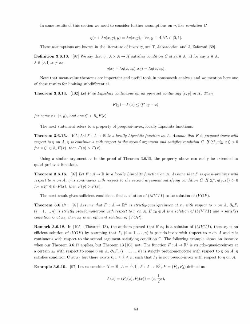
In some results of this section we need to consider further assumptions on η, like condition C:
η(x+ λη(x, y), y) = λη(x, y), ∀x, y ∈ A,∀λ ∈ [0, 1].
These assumptions are known in the literature of invexity, see T. Jabarootian and J. Zafarani [69].
Definition 3.6.13. [97] We say that η : A×A→ X satisfies condition C at x0 ∈ A iff for any x ∈ A,λ ∈ [0, 1], x 6= x0,
η(x0 + λη(x, x0), x0) = λη(x, x0).
Note that mean-value theorems are important and useful tools in nonsmooth analysis and we mention here one
of these results for limiting subdifferential.
Theorem 3.6.14. [102] Let F be Lipschitz continuous on an open set containing [x, y] in X. Then
F (y)− F (x) ≤ 〈ξ∗, y − x〉,
for some c ∈ [x, y), and one ξ∗ ∈ ∂LF (c).
The next statement refers to a property of prequasi-invex, locally Lipschitz functions.
Theorem 3.6.15. [105] Let F : A→ R be a locally Lipschitz function on A. Assume that F is prequasi-invex with
respect to η on A, η is continuous with respect to the second argument and satisfies condition C. If 〈ξ∗, η(y, x)〉 > 0
for a ξ∗ ∈ ∂LF (x), then F (y) > F (x).
Using a similar argument as in the proof of Theorem 3.6.15, the property above can easily be extended to
quasi-preinvex functions.
Theorem 3.6.16. [97] Let F : A→ R be a locally Lipschitz function on A. Assume that F is quasi-preinvex with
respect to η on A, η is continuous with respect to the second argument satisfying condition C. If 〈ξ∗, η(y, x)〉 > 0
for a ξ∗ ∈ ∂LF (x), then F (y) > F (x).
The next result gives sufficient conditions that a solution of (MV V I) to be solution of (V OP ).
Theorem 3.6.17. [97] Assume that F : A → Rn is strictly-quasi-preinvex at x0 with respect to η on A, ∂LFi
(i = 1, ..., n) is strictly pseudomonotone with respect to η on A. If x0 ∈ A is a solution of (MV V I) and η satisfies
condition C at x0, then x0 is an efficient solution of (V OP ).
Remark 3.6.18. In [105] (Theorem 13), the authors proved that if x0 is a solution of (MV V I), then x0 is an
efficient solution of (V OP ) by assuming that Fi (i = 1, . . . , n) is pseudo-invex with respect to η on A and η is
continuous with respect to the second argument satisfying condition C. The following example shows an instance
when our Theorem 3.6.17 applies, but Theorem 13 [105] not. The function F : A→ R2 is strictly-quasi-preinvex at
a certain x0 with respect to some η on A, ∂LFi (i = 1, ..., n) is strictly pseudomonotone with respect to η on A, η
satisfies condition C at x0 but there exists k, 1 ≤ k ≤ n, such that Fk is not pseudo-invex with respect to η on A.
Example 3.6.19. [97] Let us consider X = R, A = [0, 1], F : A→ R2, F = (F1, F2) defined as
F (x) = (F1(x), F2(x)) = (x,1
2x),
53
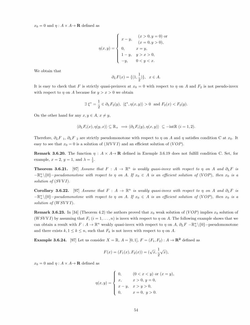
x0 = 0 and η : A×A→ R defined as
η(x, y) =
x− y,(x > 0, y = 0) or
(x = 0, y > 0),
0, x = y,
1− y, y > x > 0,
−y, 0 < y < x.
We obtain that
∂LF (x) = {(1, 1
2)}, x ∈ A.
It is easy to check that F is strictly quasi-preinvex at x0 = 0 with respect to η on A and F2 is not pseudo-invex
with respect to η on A because for y > x > 0 we obtain
∃ ξ∗ =1
2∈ ∂LF2(y), 〈ξ∗, η(x, y)〉 > 0 and F2(x) < F2(y).
On the other hand for any x, y ∈ A, x 6= y,
〈∂LFi(x), η(y, x)〉 ⊆ R+ =⇒ 〈∂LFi(y), η(x, y)〉 ⊆ −intR (i = 1, 2).
Therefore, ∂LF 1, ∂LF 2 are strictly pseudomonotone with respect to η on A and η satisfies condition C at x0. It
easy to see that x0 = 0 is a solution of (MV V I) and an efficient solution of (V OP ).
Remark 3.6.20. The function η : A × A→ R defined in Exemple 3.6.19 does not fulfill condition C. Set, for
example, x = 2, y = 1, and λ = 12 .
Theorem 3.6.21. [97] Assume that F : A → Rn is weakly quasi-invex with respect to η on A and ∂LF is
−Rn+\{0}−pseudomonotone with respect to η on A. If x0 ∈ A is an efficient solution of (V OP ), then x0 is a
solution of (SV V I).
Corollary 3.6.22. [97] Assume that F : A → Rn is weakly quasi-invex with respect to η on A and ∂LF is
−Rn+\{0}−pseudomonotone with respect to η on A. If x0 ∈ A is an efficient solution of (V OP ), then x0 is a
solution of (WSV V I).
Remark 3.6.23. In [34] (Theorem 4.2) the authors proved that x0 weak solution of (V OP ) implies x0 solution of
(WSV V I) by assuming that Fi (i = 1, . . . , n) is invex with respect to η on A. The following example shows that we
can obtain a result with F : A→ Rn weakly quasi-invex with respect to η on A, ∂LF −Rn+\{0}−pseudomonotone
and there exists k, 1 ≤ k ≤ n, such that Fk is not invex with respect to η on A.
Example 3.6.24. [97] Let us consider X = R, A = [0, 1], F = (F1, F2) : A→ R2 defined as
F (x) = (F1(x), F2(x)) = (√x,
1
2
√x),
x0 = 0 and η : A×A→ R defined as
η(x, y) =
0, (0 < x < y) or (x = y),
x, x > 0, y = 0,
x− y, x > y > 0,
0, x = 0, y > 0.
54
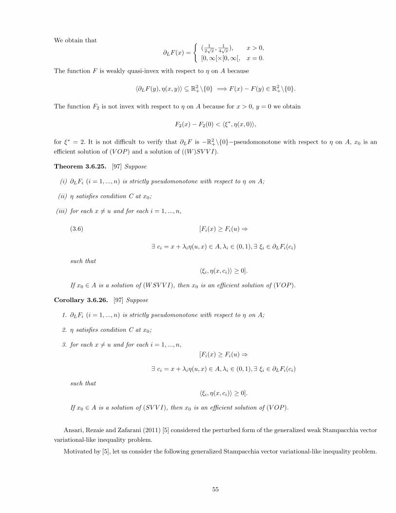
We obtain that
∂LF (x) =
{( 1
2√x, 1
4√x
), x > 0,
[0,∞[×[0,∞[, x = 0.
The function F is weakly quasi-invex with respect to η on A because
〈∂LF (y), η(x, y)〉 ⊆ R2+\{0} =⇒ F (x)− F (y) ∈ R2
+\{0}.
The function F2 is not invex with respect to η on A because for x > 0, y = 0 we obtain
F2(x)− F2(0) < 〈ξ∗, η(x, 0)〉,
for ξ∗ = 2. It is not difficult to verify that ∂LF is −R2+\{0}−pseudomonotone with respect to η on A, x0 is an
efficient solution of (V OP ) and a solution of ((W )SV V I).
Theorem 3.6.25. [97] Suppose
(i) ∂LFi (i = 1, ..., n) is strictly pseudomonotone with respect to η on A;
(ii) η satisfies condition C at x0;
(iii) for each x 6= u and for each i = 1, ..., n,
(3.6) [Fi(x) ≥ Fi(u)⇒
∃ ci = x+ λiη(u, x) ∈ A, λi ∈ (0, 1),∃ ξi ∈ ∂LFi(ci)
such that
〈ξi, η(x, ci)〉 ≥ 0].
If x0 ∈ A is a solution of (WSV V I), then x0 is an efficient solution of (V OP ).
Corollary 3.6.26. [97] Suppose
1. ∂LFi (i = 1, ..., n) is strictly pseudomonotone with respect to η on A;
2. η satisfies condition C at x0;
3. for each x 6= u and for each i = 1, ..., n,
[Fi(x) ≥ Fi(u)⇒
∃ ci = x+ λiη(u, x) ∈ A, λi ∈ (0, 1),∃ ξi ∈ ∂LFi(ci)
such that
〈ξi, η(x, ci)〉 ≥ 0].
If x0 ∈ A is a solution of (SV V I), then x0 is an efficient solution of (V OP ).
Ansari, Rezaie and Zafarani (2011) [5] considered the perturbed form of the generalized weak Stampacchia vector
variational-like inequality problem.
Motivated by [5], let us consider the following generalized Stampacchia vector variational-like inequality problem.
55
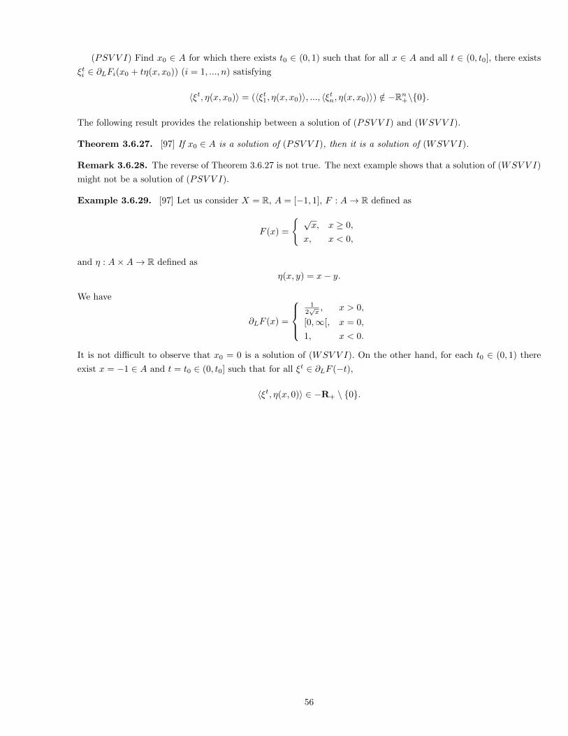
(PSV V I) Find x0 ∈ A for which there exists t0 ∈ (0, 1) such that for all x ∈ A and all t ∈ (0, t0], there exists
ξti ∈ ∂LFi(x0 + tη(x, x0)) (i = 1, ..., n) satisfying
〈ξt, η(x, x0)〉 = (〈ξt1, η(x, x0)〉, ..., 〈ξtn, η(x, x0)〉) /∈ −Rn+\{0}.
The following result provides the relationship between a solution of (PSV V I) and (WSV V I).
Theorem 3.6.27. [97] If x0 ∈ A is a solution of (PSV V I), then it is a solution of (WSV V I).
Remark 3.6.28. The reverse of Theorem 3.6.27 is not true. The next example shows that a solution of (WSV V I)
might not be a solution of (PSV V I).
Example 3.6.29. [97] Let us consider X = R, A = [−1, 1], F : A→ R defined as
F (x) =
{ √x, x ≥ 0,
x, x < 0,
and η : A×A→ R defined as
η(x, y) = x− y.
We have
∂LF (x) =
1
2√x, x > 0,
[0,∞[, x = 0,
1, x < 0.
It is not difficult to observe that x0 = 0 is a solution of (WSV V I). On the other hand, for each t0 ∈ (0, 1) there
exist x = −1 ∈ A and t = t0 ∈ (0, t0] such that for all ξt ∈ ∂LF (−t),
〈ξt, η(x, 0)〉 ∈ −R+ \ {0}.
56
Bibliography
[1] S. Al-Homidan, Q.H. Ansari, Generalized Minty vector variational-like inequalities and vector optimization
problems, J. Optim. Theory Appl., 144 (2010), 1-11.
[2] M.H. Alizadeh, N. Hadjisavvas, M. Roohi, Local boundedness and surjectivity properties for generalized mono-
tone operators, Private communication.
[3] Q.H. Ansari, G.M. Lee, Nonsmooth vector optimization problems and Minty vector variational inequalities, J.
Optim. Theory Appl., 145(1) (2010), 1-16.
[4] Q.H. Ansari, M. Rezaie, Existence results for Stampacchia and Minty type vector variational inequalities,
Optimization 59(7) (2010), 1053-1065.
[5] Q.H. Ansari, M. Rezaie, J. Zafarani, Generalized variational-like inequalities and vector optimization, J. Global
Optim. 53(2) (2011), 271-284
[6] Q.H. Ansari, J.-K. Yao, Recent Developments on Vector Optimization, Springer, Berlin, 2012.
[7] Q.H. Ansari, X.C. Yang, J.C. Yao, Existence and duality of implicit vector variational problems, Numer. Funct.
Anal. Optim., 2002.
[8] Q.H. Ansari, S. Schaible, J.C. Yao, System of vector equilibrium problems and its applications, J. Optim. Theory
Appl. 107 (2000), 547-557.
[9] Staib, T., On two generalizations of Pareto minimality, J. Optim. Theory Appl. 59 2 (1988), 289-306.
[10] J.P. Aubin, Mathematical Methods of Game and Economic Theory, North Holland, Amsterdam, 1979.
[11] J.P. Aubin, H. Frankowska, Set-valued Analysis, Birkhauser, Boston, 1990.
[12] T. Basar, G.J. Olsder, Dynamic Noncooperative Game Theory (second edition), SIAM, Philadelphia, 1999.
[13] T.Q. Bao, B.S. Mordukhovich, Relative Pareto minimizer to multiobjective problems: Existence and optimality
conditions, Math. Program. 122 (2010), 301-347.
[14] L.B. Batista Dos Santos, G. Ruiz-Garzon, M.A. Rojas-Medar, A. Rufian-Lizana, Some relations between
variational-like inequality problems and vector optimization problems in Banach spaces, Comput. Math. Appl.
55 (2008), 1808-1814.
[15] H.H. Bauschke, P.L. Combettes, Convex Analysis and Monotone Operator Theory in Hilbert Spaces, Springer,
New York Dordrecht Heidelberg London, 2011.
[16] M. Bianchi, S. Schaible, Generalized monotone bifunctions and equilibrium problems, J. Optim. Theory Appl.
90 (1996), 31-43.
57
[17] M. Bianchi, N. Hadjisavvas, S. Schaible, Vector equilibrium problems with generalized monotone bifunctions, J.
Optim. Theory Appl. 92 (1997), 527-542.
[18] M. Bianchi, R. Pini, A note on equilibrium problems with properly quasimonotone bifunctions, J. Global Optim.
20 (2001), 67-76.
[19] M. Bianchi, R. Pini, Coercivity conditions for equilibrium problems, J. Optim. Theory Appl. 124 (2005), 79-92.
[20] M. Bianchi, G. Kassay, R. Pini, Existence of equilibria via Ekeland’s principle, J. Math. Anal. Appl. 305 (2005),
502-512.
[21] G. Bigi, M. Castellani, G. Kassay, A dual view of equilibrium problems, J. Math. Anal. Appl. 342 (2008), 17-26.
[22] E. Blum, W. Oettli, From optimization and variational inequalities to equilibrium problems, Math. Stud. 63
(1994), 123-145.
[23] H. Brezis, G. Nirenberg, G. Stampacchia, A remark on Ky Fan’s minimax principle, Bollettino U.M.I. 6 (1972),
293-300.
[24] H. Brezis, Equations et inequations non lineaires dans les espaces vectorieles en dualite, Ann. Inst. Fourier 18
(1968), 115-175.
[25] F.E. Browder, Multi-valued monotone nonlinear mappings, Trans. Amer. Math. Soc. 118 (1965), 338-551.
[26] F.E. Browder, Nonlinear maximal monotone mappings in Banach spaces, Math. Ann. 175 (1968), 81-113.
[27] F.E. Browder, P. Hess, Nonlinear mappings of monotone type in Banach spaces, J. Funct. Anal. 11 (1972),
251-294.
[28] R.S. Burachik, A.N. Iusem, Set-Valued Mappings and Enlargements of Monotone Operators, Springer, Berlin,
2007.
[29] A. Cambini, L. Martein, Handbook of Generalized Convexity and Generalized Monotonicity, In: Nonconvex
Optimization and Its Applications, vol. 76, Springer, The Netherlands, 2005.
[30] A. Capata, G. Kassay, On vector equilibrium problems and applications, Taiwanese J. Math. 15 (2011), 365-380.
[31] O. Chadli, Y. Chiang, S. Huang, Topological pseudomonotonicity and vector equilibrium problems, J. Math.
Anal. Appl. 270 (2002), 435-450.
[32] S.S. Chang, Y. Zhang, Generalized KKM theorem and variational inequalities, J. Math. Anal. Appl. 159 (1991),
208-223.
[33] G.-Y. Chen, Q.M. Cheng, Vector variational inequality and vector optimization, in: Y. Sawaragi, K. Inoue
and H. Nakayama (eds.), Towards Interactive and Intelligent Decision Support Systems, Springer-Verlag, New
York, 1987, 408-416.
[34] B. Chen, N.J. Huang, Vector variational-like inequalities and vector optimization problems in Asplund spaces,
Optim. Lett., 6(7) (2012), 1513-1525.
[35] G.-Y. Chen, S.H. Hou, Existence of solutions for vector variational inequalities, in: F. Giannessi (ed.), Vector
Variational Inequalities and Vector Equilibria, Kluwer Academic Publishers, Dordrecht 2000, 73-86.
[36] Y. Chiang, Vector superior and inferior, Taiwanese J. Math. 8(3) (2004), 477-487.
58
[37] A. Chinchuluun, P.M. Pardalos, A survey of recent developments in multiobjective optimization, Ann. Oper.
Res. 154(1) (2007), 29-50.
[38] B.D. Craven, Mathematical Programming and Control Theory, Chapman and Hall, London, 1978.
[39] A. Daniilidis, N. Hadjisavvas, On generalized cyclically monotone operators and proper quasimonotonicity,
Optimization 47 (2000), 123-135.
[40] A. Domokos, J. Kolumban, Comparison of two different types of pseudomonotone mappings, In: Seminaire de
la theorie de la meilleure approximation, convexite et optimisation, Cluj-Napoca, 2000, 95-103.
[41] M. Eidelheit, Zur Theorie der konvexen Mengen in linearen normierten Raumen, Studia Math. 6 (1936),
104-111.
[42] I. Ekeland, On the variational principle, J. Math. Anal. Appl. 47 (1974), 324-353.
[43] K. Fan, Minimax theorems, Proc. Nat. Acad. Sci. U.S.A. 39 (1953), 42-47.
[44] K. Fan, A generalization of Tychonoff’s fixed point theorem, Math. Ann. 142 (1961), 305-310.
[45] K. Fan, Application of a theorem concerning sets with convex sections, Math. Ann. 163 (1966), 189-203.
[46] K. Fan, A minimax inequality and applications, In: Inequalities, Vol. III, O. Shisha (Ed.), Academic Press
1972, 103-113.
[47] Y.P. Fang, N.J. Huang, Strong vector variational inequalities in Banach spaces, Appl. Math. Lett. 19 (2006),
362-368.
[48] Y.P. Fang, N.J. Huang, Existence results for generalized implicit vector variational inequalities with multivalued
mappings, Indian J. Pure Appl. Math. 36 (2005), 629-640.
[49] A.P. Farajzadeh, A.A. Harandi, K.R. Kazmi, Existence of solutions to generalized vector variational-like in-
equalities, J. Optim. Theory Appl. 146 (2010), 95-104.
[50] F. Ferro, A minimax theorem for vector-valued functions, J. Optim. Theory Appl. 60 (1989), 19-31.
[51] C. Finet, L. Quarta, C. Troestler, Vector-valued variational principles, Nonlinear Anal. 52 (2003), 197-218.
[52] G.R. Garzon, R.O. Gomez, A.R. Lizana, Generalized invex monotonicity, Eur. J. Oper. Res. 144 (2003),
501-512.
[53] G.R. Garzon, R.O. Gomez, A.R. Lizana, Relationship between vector variational-like inequality and optimization
problems, Eur. J. Oper. Res. 157 (2004), 113-119.
[54] F. Giannessi, On Minty variational principle, In: Giannessi, F., Komlosi, S., TapKsaKk, T. (eds.) New Trends
in Mathematical Programming, Kluwer Academic, Dordrecht, 1998, 93-99.
[55] F. Giannessi, Vector Variational Inequalities and Vector Equilibria: Mathematical Theories, Kluwer Academic,
Dordrecht, 2000.
[56] F. Giannessi, A. Maugeri, P.M. Pardalos, Equilibrum Problems: Nonsmooth Optimization and Variational
Inequalities Models, Springer, Berlin, 2002.
[57] X.H. Gong, Optimality conditions for vector equilibrium problems, J. Math. Anal. Appl. 342 (2008), 1455-1466.
59
[58] N. Hadjisavvas, Generalized Convexity, Generalized Monotonicity and Nonsmooth Analysis, In: Handbook
of Generalized Convexity and Monotonicity, Series: Nonconvex Optimization and its Applications, Vol. 76,
Hadjisavvas, Nicolas; Komlosi, Sandor; Schaible, Siegfried (Eds.), Springer, Berlin-Heidelberg-New York, 2005,
3-87.
[59] N. Hadjisavvas, S. Schaible, From scalar to vector equilibrium problems in the quasimonotone case, J. Optim.
Theory Appl. 96 (1998), 297-309.
[60] M.A. Hanson, On sufficienty of the Kuhn-Tucker conditions, J. Math. Anal. Appl. 80 (1981), 545-550.
[61] R. Hartley, On cone-efficiency, cone-convexity and cone-compactness, SIAM J. Appl. Math. 34 (1978), 211-222.
[62] S.H. Hu, N.S. Papageorgiu, Handbook of Multivalued Analysis, vol. I, Kluwer, 1997.
[63] D. Inoan, J. Kolumban, On pseudomonotone set-valued mappings, Nonlinear Anal. 68 (2008), 47-53.
[64] A.N. Iusem, W. Sosa, New existence results for equilibrium problems, Nonlinear Anal. 52 (2003), 621-635.
[65] A.N. Iusem, W. Sosa, Iterative algorithms for equilibrium problems, Optimization 52 (2003), 301-316.
[66] A.N. Iusem, G. Kassay, W. Sosa, An existence result for equilibrium problem with some surjectivity conse-
quences, J. Convex Anal. 16 (2009), 807-826.
[67] A.N. Iusem, G. Kassay, W. Sosa, On certain conditions for the existence of solutions of equilibrium problems,
Math Prog. 116 (2009), 259-273.
[68] J. Jahn, Vector Optimization: Theory, Applications, and Extensions, Springer-Verlag, Berlin, 2004.
[69] T. Jabarootian, J. Zafarani, Generalized invariant monotonicity and invexity of non-differentiable functions,
J. Global Optim. 36 (2006), 537-564.
[70] V. Jeyakumar, Convexlike alternative theorems and mathematical programming, Optimization 16 (1985), 643-
652.
[71] V. Jeyakumar, A generalization of a minimax theorem of Fan via a theorem of the alternative, J. Optim. Theory
Appl. 48 (1986), 525-533.
[72] A.J. Jones, Game theory: Mathematical Models of Conflict, Horwood Publishing, Chicester, 2000.
[73] S. Karamardian, Complementarity problems over cones with monotone and pseudomonotone maps, J. Optim.
Theory Appl. 18 (1976), 445-454.
[74] S. Karamardian, S. Schaible, Seven kinds of monotone maps, J. Optim. Theory Appl. 66 (1990), 37-46.
[75] P. Kas, G. Kassay, Z. Boratas-Sensoy, On generalized equilibrium points, J. Math. Anal. Appl. 296 (2004),
619-633.
[76] G. Kassay, The Equilibrium Problem and Related Topics, Risoprint, Cluj-Napoca, 2000.
[77] G. Kassay, J. Kolumban, On a generalized sup-inf problem, J. Optim. Theory Appl. 91 (1996), 651-670.
[78] G. Kassay, M. Miholca, Existence results for variational inequalities with surjectivity consequences related to
generalized monotone operators, J. Optim. Theory Appl. 159 (2013), 721-740.
[79] G. Kassay, M. Miholca, On vector equilibrium problems given by a sum of two functions, submitted.
60
[80] K.R. Kazmi, On Vector equilibrium problem, Proc. Indian Acad. Sci. 110 (2000), 213-223.
[81] B.T. Kien, The normalized duality mapping and two related characteristic properties of a uniformly convex
Banach space, Acta Math. Vietnamica 27 (2002), 53-67.
[82] M.D. Kirszbraun, Uber die Zusammenziehenden und Lipschitzschen Transformationen, Fund. Math. 22 (1934),
7-10.
[83] B. Knaster, C. Kuratowski, S. Mazurkiewicz, Ein Beweis des Fixpunktsatzes fur n-dimensionale Simplexe,
Fund. Math. 14 (1929), 132-138.
[84] J. Kolomy, Maximal monotone mappings in Banach spaces, Acta Univ. Carolinae - Math. et Phys. 33 (1992),
63-67.
[85] S. Komlosi, Generalized Monotonicity in Nonsmooth Analysis, In: Generalized Convexity, S. Komlosi, T.
Rapcsak, S. Schaible (Eds.), Springer-Verlag 1994, 263-275.
[86] H. Konig, Uber das von Neumannsche minimax-theorem, Archiv der Mathematik 19 (1968), 482-487.
[87] I. Konnov, Generalized monotone equilibrum problems and variational inequalities, In: Handbook of Generalized
Convexity and Monotonicity, Series: Nonconvex Optimization and its Applications, Vol. 76, Hadjisavvas,
Nicolas; Komlosi, Sandor; Schaible, Siegfried (Eds.), Springer, Berlin-Heidelberg-New York 2005, 559-618.
[88] I.V. Konnov, J.C. Yao, Existence of solutions for generalized vector equilibrium problems, J. Math. Anal. Appl.
233 (1999), 328-335.
[89] I. Konnov, D.T. Luc, A.M. Rubinov (eds.), Generalized Convexity and Related Topics, Springer-Verlag, Berlin,
2007.
[90] H.W. Kuhn, Lectures on the Theory of Games, Princeton University Press, Princeton, 2003.
[91] K.L. Lin, D.P. Yang, J.C. Yao, Generalized vector variational inequalities, J. Optim. Theory Appl. 92 (1997),
117-125.
[92] A. Lohne, Vector Optimization with Infimum and Supremum, Springer, 2011.
[93] D.T. Luc, Theory of Vector Optimization, Springer-Verlag, Berlin, 1989.
[94] A. Maugeri, F. Raciti, On existence theorems for monotone and nonmonotone variational inequalities, J.
Convex Anal. 16 (2009), 899-911.
[95] M. Miholca, Vector variational-like inequalities and set-valued optimization problems, Ann. of Tiberiu Popoviciu
Seminar 10 (2012), 75-85.
[96] M. Miholca, On set-valued optimization problems and vector variational-inequalities, Optim. Lett. 8(2) (2014),
463-476.
[97] M. Miholca, Vector variational-like inequalities and vector optimization problems, Carpathian J. Math. 30(1)
(2014), 101-108.
[98] M. Miholca, Lipschitz B-preinvex functions in Asplund spaces, submitted.
[99] M. Miholca, On vector variational-like inequalities and vector optimization problems in Asplund spaces, accepted
for publication in Studia Mathematica Universitatis Babes-Bolyai.
61
[100] G.J. Minty, Monotone (nonlinear) operators in Hilbert spaces, Duke Math. J. 29 (1962), 341-346.
[101] S.K. Mishra, S.Y. Wang, Vector variational-like inequalities and non-smooth vector optimization problems,
Nonlinear Anal. 64 (2006), 1939-1945.
[102] B. Mordukhovich, Variations Analysis and Generalized Differentation, I: Basic Theory, Grundlehren series
(fundamental principles of mathematical sciences) 330, Springer, Berlin, 2006.
[103] I. Muntean, Functional Analisys (Romanian), Babes-Bolyai University, Cluj, 1973.
[104] W. Oettli, A remark on vector-valued equilibria and generalized monotonicity, Acta Math. Vietnam. 22 (1997),
215-221.
[105] M. Oveisiha, J. Zafarani, Vector optimization problem and generalized convexity, J. Global Optim., 52(1)
(2011), 29-43.
[106] S. Paeck, Convexlike and concavelike conditions in alternative, minimax, and minimization theorems, J. Op-
tim. Theory Appl. 74 (1992), 317-332.
[107] P.M. Pardalos, T.M. Rassias, A.A. Khan, Nonlinear Analysis and Variational Problems, Springer, Berlin,
2010.
[108] R. Pini, Invexity and generalized convexity, Optimization 22 (1991), 513-525.
[109] N. Popovici, Vector Optimization (Romanian), Casa Cartii de Stiinta, Cluj-Napoca, 2005.
[110] M. Rezaie, J. Zafarani, Vector optimization and variational-like inequalities, J. Global Optim. 43 (2009),
47-66.
[111] R.T. Rockafellar, Convex Analysis, Princeton University Press, Princeton, 1970.
[112] H.L. Royden, Real Analysis (third edition), Macnmillan Publishing Company, New York, 1988.
[113] W. Rudin, Principles of Mathematical Analysis, McGraw-Hill, New York, 1976.
[114] W. Rudin, Functional Analysis, T. M. H. Edition, New Delhi, 1976.
[115] J. Schauder, Der Fixpunktsatz in Funktionalraumen, Studia Math. 2 (1930), 171-180.
[116] M. Soleimani-damaneh, Characterizations and applications of generalized invexity and monotonicity in As-
plund spaces, Top. 20(2012), 592-613.
[117] M. Soleimani-damaneh, Characterization of nonsmooth quasiconvex and pseudoconvex functions, J. Math.
Anal. Appl. 330 (2007), 1387-1392.
[118] T. Tanaka, Generalized semicontinuity and existence theorems for cone saddle points, Appl. Math. Optim. 36
(1997), 313-322.
[119] J. Von Neumann, Zur theorie der gesellschaftsspiele, Math. Ann. 100 (1928), 295-320.
[120] N.N. Vorob’ev, Game theory: Lectures for Economists and Systems Scientists, Springer, New York, 1977.
[121] J.C. Yao, Multi-valued variational inequalities with K-pseudomonotone operators, J. Optim. Theory Appl. 83
(1994), 391-403.
62
[122] X.M. Yang, X.Q. Yang, Vector variational-like inequalities with pseudoinvexity, Optimization 55 (2006), 157-
170.
[123] X.M. Yang, X.Q. Yang, K.L. Teo, Generalized invexity and generalized invariant monotonicity, J. Optim.
Theory Appl. 117 (2003), 607-625.
[124] X.M. Yang, X.Q. Yang, K.L. Teo, Criteria for generalized invex monotonicity, Eur. J. Oper. Res. 164 (2005),
115-119.
[125] X.M. Yang, X.Q. Yang, K.L. Teo, Some remarks on the Minty vector variational inequality, J. Optim. Theory
Appl. 121 (2004), 193-201.
[126] X.M. Yang, X.Q. Yang, K.L. Teo, Generalizations and applications of prequasi-invex functions, J. Optim.
Theory Appl. 110 (2001), 645-668.
[127] K. Yosida, Functional Analysis, Springer-Verlag, Berlin-Heidelberg, 1980.
[128] E. Zeidler, Nonlinear Functional Analysis and its Applications II/B, Nonlinear Monotone Operators, Springer-
Verlag, New York, 1990.
[129] J. Zeng, S.J. Li, On vector variational-like inequalities and set-valued optimization problems, Optim. Lett.
5(1) (2011), 55-69.
[130] J.X. Zhou, G. Chen, Diagonal convexity conditions for problems in convex analysis and quasi-variational
inequalities, J. Math. Anal. Appl. 132 (1998), 213-225.
63