Continuum thermodynamics of ferroelectric domain …landis/Landis/Research_files/JMPS2007.pdfContinuum thermodynamics of ferroelectric domain evolution: Theory, ﬁnite element

ARTICLE IN PRESS

Journal of the Mechanics and Physics of Solids

55 (2007) 280–305

0022-5096/$ -

doi:10.1016/j

�CorrespoE-mail ad

www.elsevier.com/locate/jmps

Continuum thermodynamics of ferroelectric domainevolution: Theory, finite element implementation,

and application to domain wall pinning

Yu Su, Chad M. Landis�

Department of Mechanical Engineering and Materials Science, MS 321, Rice University, P.O. Box 1892,

Houston, TX 77251-1892, USA

Received 18 April 2006; received in revised form 11 July 2006; accepted 17 July 2006

Abstract

A continuum thermodynamics framework is devised to model the evolution of ferroelectric

domain structures. The theory falls into the class of phase-field or diffuse-interface modeling

approaches. Here a set of micro-forces and governing balance laws are postulated and applied within

the second law of thermodynamics to identify the appropriate material constitutive relationships.

The approach is shown to yield the commonly accepted Ginzburg–Landau equation for the

evolution of the polarization order parameter. Within the theory a form for the free energy is

postulated that can be applied to fit the general elastic, piezoelectric and dielectric properties of a

ferroelectric material near its spontaneously polarized state. Thereafter, a principle of virtual work is

specified for the theory and is implemented to devise a finite element formulation. The theory and

numerical methods are used to investigate the fields near straight 1801 and 901 domain walls and to

determine the electromechanical pinning strength of an array of line charges on 1801 and 901 domain

walls.

r 2006 Elsevier Ltd. All rights reserved.

Keywords: Ferroelectrics; Phase-field modeling; Finite element methods; Piezoelectrics; Domain switching

see front matter r 2006 Elsevier Ltd. All rights reserved.

.jmps.2006.07.006

nding author. Tel.: +713 348 3609; fax: +713348 5423.

dress: [email protected] (C.M. Landis).

www.elsevier.com/locate/jmps

dx.doi.org/10.1016/j.jmps.2006.07.006

mailto:[email protected]

ARTICLE IN PRESSY. Su, C.M. Landis / J. Mech. Phys. Solids 55 (2007) 280–305 281

1. Introduction

Ferroelectric ceramics are being increasingly used in macro- and micro-deviceapplications for actuators, sensors, and information storage. The fundamental behaviorutilized in these devices is the strong electro-mechanical coupling exhibited by theferroelectric material. In order to predict the performance and reliability of such devices itis necessary to understand the mechanics and physics governing the constitutive responseof the ferroelectric material at the appropriate scales. The primary mechanism responsiblefor nonlinear ferroelectric constitutive response at practically all scales is the motion ofdomain walls. There is also evidence that the attractive ‘‘linear’’ properties of manyferroelectrics, such as high piezoelectric constants and large dielectric constants, is due toanelastic domain wall motion (Xu et al., 2005). The nature of domain walls and theirinteractions with other material defects is fundamental to the understanding of the physicalphenomena associated with the finite coercive strength of ferroelectrics, fracturetoughening associated with domain switching (Wang and Landis, 2004), and electricalfatigue associated with pinning of domain walls by migrating charge carriers (Warren etal., 1994; Xiao et al., 2005).

In this paper, a continuum thermodynamics framework is presented to model theevolution of ferroelectric domain structures. The theory falls into the class of phase-field ordiffuse-interface modeling approaches (Cao and Cross, 1991; Nambu and Sagala, 1994;Hu and Chen, 1997; Ahluwalia and Cao, 2000, 2001; Li et al., 2001, 2002; Wang et al.,2004; Zhang and Bhattacharya, 2005a, b), which has the potential to bridge atomisticcalculations (Cohen and Krakauer, 1992; Meyer and Vanderbilt, 2002) and the larger scalephenomenological modeling approaches. In a departure from previous derivations of thephase-field equations, a set of micro-forces and governing balance laws are postulated andapplied within the second law of thermodynamics to identify the appropriate materialconstitutive relationships (Fried and Gurtin, 1993, 1994; Gurtin, 1996). The approach isshown to yield the commonly accepted Ginzburg–Landau equation for the evolution of theelectrical polarization order parameter. Within the theory a form for the free energy ispostulated that can be applied to fit the general elastic, piezoelectric, and dielectricproperties of a ferroelectric material near its spontaneously polarized state. To investigatethe consequences of the theory simple planar domain wall motions are analyzed.Thereafter, a principle of virtual work is specified for the theory and is implemented todevise a finite element formulation. The theory and numerical methods are used toinvestigate the interactions of 1801 and 901 domain walls with arrays of charged defectsand to determine how strongly domain walls are electromechanically pinned by the arraysof defects.

The outline of the remainder of the paper is as follows. In Section 2 the governingequations for the theory are presented, including a new micro-force balance and theconsequences associated with the second law of thermodynamics. In Section 3 someanalytical results associated with straight domain walls are given along with numericalresults for the fields near 1801 and 901 domain walls for material parameters that modelBaTiO3. Section 4 develops a finite element formulation that can be used to numericallysolve the model equations in higher dimensions. Section 5 formulates the problem of adomain wall interacting with an array of uniformly spaced line charges. Numerical finiteelement results are presented for the equilibrium domain wall shapes near the array and forthe critical sets of electromechanical fields required to break through the array. The results

ARTICLE IN PRESSY. Su, C.M. Landis / J. Mech. Phys. Solids 55 (2007) 280–305282

are discussed within the context of the coercive electromechanical ‘‘strength’’ of singlecrystals. Finally, Section 6 offers a discussion of the model and future avenues of study.

2. Theory

If one is given a static domain structure then the equations governing the distributions ofelectromechanical fields in the material based on linear piezoelectricity are well established,and there exists several numerical techniques that can be applied to solve for these fields(Allik and Hughes, 1970; Landis, 2002a). However, we are not only interested in thedistribution of the fields, but also in how these fields cause the domain structure to evolve.Hence, this problem falls into a broader class of free boundary problems where thelocations of the interfaces must also be determined as part of the solution. A sharpinterface approach could be applied, but contains physical questions associated withspecial rules for nucleation, and numerical concerns associated with changes in topology ofthe domain structure. In order to circumvent the challenges associated with a sharpinterface approach, a diffuse-interface or ‘‘phase-field’’ methodology is taken here.Traditionally, the phase-field equations governing the evolution of domain configura-

tions have been derived from a simple and physically justifiable set of assumptions. Whilethis approach is certainly sound, it obscures the modern continuum physics distinctionbetween fundamental balance laws, which are applicable to a wide range of materials, andthe constitutive equations that are valid for a specific material (Fried and Gurtin, 1993,1994; Gurtin, 1996). Here we present a small deformation non-equilibrium thermo-dynamics framework for ferroelectric domain evolution. We begin with the fundamentalequations governing the electromechanical fields under the assumption of smalldeformations and rotations. Note that the small deformation assumption is prevalentthroughout the phase-field modeling literature. The analysis of large deformations wouldintroduce the concept of Maxwell stresses (Toupin, 1956; McMeeking and Landis, 2005),which are assumed to be higher order effects that can be neglected. Following previousphase-field modeling approaches, the effects of large deformations will not be consideredhere, but their incorporation within the theory is possible. It will also be assumed that thefields vary slowly with respect to the speed of light in the material, i.e. the quasi-staticelectromagnetic field approximation, but not necessarily with respect to the speed ofsound, i.e. inertial effects are considered within the general derivation. Specifically,balances of linear and angular momentum in any arbitrary volume V and its boundingsurfaces S yield

sji;j þ bi ¼ r €ui in V , (2.1)

sij ¼ sji in V , (2.2)

sjinj ¼ ti on S, (2.3)

where sij are the Cartesian components of the Cauchy stress, bi the components of a bodyforce per unit volume, r the mass density, ui the mechanical displacements, ni thecomponents of a unit vector normal to a surface element, and ti the tractions applied to thesurface. Standard index notation is used with summation implied over repeated indices, thedouble overdot represents a second derivative with respect to time, and the subscript, j

represents partial differentiation with respect to the xj coordinate direction. Under the


assumptions of linear kinematics, the strain components eij are related to the displacementsas

�ij ¼12ðui;j þ uj;iÞ in V . (2.4)

The electrical quantities of electric field, Ei; electric potential, f; electric displacement, Di;volume charge density, q; and surface charge density, o; are governed by the quasi-staticforms of Maxwell’s equations. Specifically, in any arbitrary volume V (including a regionof free space) and its bounding surface S,

Di;i � q ¼ 0 in V , (2.5)

Dini ¼ �o on S, (2.6)

Ei ¼ �f;i in V . (2.7)

Within the theory of linear piezoelectricity, Eqs. (2.1)–(2.7) represent the fundamentalbalance laws and kinematic relationships, and the constitutive laws required to close theloop on the equations relate the stress and electric field to the strain and electricdisplacement. Such constitutive relationships can be derived from thermodynamicconsiderations using a material free energy that depends on the components of the strainand electric displacement (Nye, 1957). However, within the phase-field modeling approachthe free energy will also be required to depend on an order parameter and its gradient.Mathematically, the order parameter is used to describe the different material varianttypes, i.e. the spontaneous states that are possible in a crystal. For the case of ferroelectrics,the physically natural order parameter is the electrical polarization Pi. Note thatthe relationship between electric field, electric displacement and material polarization isgiven as

Di ¼ Pi þ k0Ei in V . (2.8)

Here k0 is the permittivity of free space. Given that the free energy will be allowed todepend on a new independent variable Pi, we must now allow for a new system of ‘‘micro-forces’’ that are work conjugate to this configurational quantity. Following the work (andwording) of Fried and Gurtin (1993, 1994), and Gurtin (1996) we introduce a micro-forcetensor xji such that xjinj

_Pi represents a power density expended across surfaces byneighboring configurations, an internal micro-force vector pi such that pi

_Pi is the powerdensity expended by the material internally, e.g. in the ordering of atoms within unit cellsof the lattice (this micro-force will account for dissipation in the material), and an externalmicro-force vector gi such that gi

_Pi is a power density expended on the material by externalsources. Then, the integral balance of this set of configurational forces leads to thedifferential balance lawZ

S

xjinj dS þ

ZV

pi dV þ

ZV

gi dV ¼ 0) xji;j þ pi þ gi ¼ 0 in V . (2.9)

To remain as general as possible, it is assumed that the Helmholtz free energy of thematerial (including the free space occupied by the material) takes the following form:

c ¼ c �ij ;Di;Pi;Pi;j ; _Pi

� �. (2.10)

Note that temperature plays a key role in ferroelectric phase transitions near the Curiepoint. For isothermal behavior, the Helmholtz free energy remains the appropriate energy


functional with the additional complication that the material parameters of the free energyare temperature dependent (Devonshire, 1954; Jona and Shirane, 1962). Here we will dealonly with constant temperature behavior below the Curie temperature, but recognize thatthe extension to spatially homogeneous temperature-dependent behavior can be readilyincluded within the present framework simply by specifying the temperature at which thematerial properties must be evaluated. In contrast, the inclusion of spatially inhomogeneous

temperature-dependent behavior and the associated thermal diffusion requires an analysisof the second law of thermodynamics including such effects, and would call for theintroduction of temperature and entropy as additional field variables within the theory andnumerical treatment. In the following, only the constant temperature cases will beconsidered.For the isothermal processes below the Curie temperature under consideration, the

second law of thermodynamics is written as the Clausius–Duhem (dissipation) inequalityas Z

V

_cdV þd

dt

ZV

1

2r _ui _ui dVp

ZV

ðbi _ui þ f _qþ gi_PiÞdV þ

ZS

ðti _ui þ f _oþ xjinj_PiÞdS.

(2.11)

Here the left-hand side represents the rate of stored plus kinetic energy in the material andthe right-hand side represents the power expended by external sources on the body. Notethat the internal micro-force pi does not contribute to this external power term.Substitution into (2.11) of the balance laws of Eqs. (2.1)–(2.9), along with the applicationof the divergence theorem yieldsZ

V

qcq�ij

_�ij þqcqDi

_Di þqcqPi

_Pi þqcqPi;j

_Pi;j þqcq _Pi

€Pi dV

pZ

V

sji_�ij þ Ei_Di þ xji

_Pi;j � pi_Pi dV . ð2:12Þ

Note that the assumption implicit to Eq. (2.10) is that the stress, electric field, micro-forcetensor, and internal micro-force each are allowed to depend on eij, Di, Pi, Pi,j, and _Pi. Thequestion can be raised as to why the free energy must be allowed to depend on _Pi. Theanswer being that since the internal micro-force pi is allowed to depend on _Pi, then all ofthe thermodynamic forces must also potentially have such dependence (Coleman and Noll,1963). It will be shown that the second law inequality ultimately allows only pi to dependon _Pi (see Eqs. (2.13) and (2.14)). Following Coleman and Noll (1963), it is assumed thatfor a given thermodynamic state, arbitrary levels of _�ij ; _Di; _Pi; _Pi;j ; and €Pi are permissiblethrough the appropriate control of the external sources bi, q, and gi. Then, given thatEq. (2.12) must hold for all permissible processes, an analysis of the dissipation inequalityimplies that

qcq _Pi

¼ 0) c ¼ c �ij ;Di;Pi;Pi;j

� �, (2.13)

sji ¼qcq�ij

; Ei ¼qcqDi

; and xji ¼qcqPi;j

. (2.14)


Finally, after defining Zi � (qc/qPi), the internal micro-force pi must satisfy

pi þ Zi

� �_Pip0) pi ¼ �Zi � bij

_Pj

with bij ¼ bij �kl ;Dk;Pk;Pk;l ; _Pk

� �positive definite: ð2:15Þ

If the inverse ‘‘mobility’’ tensor b is constant and the high-temperature phase is cubic thenbij ¼ bdij where bX0. This is the simplest and most widely applied form for bij.Substitution of Eqs. (2.14c) and (2.15) into the micro-force balance of Eq. (2.9) yields ageneralized form of the Ginzburg–Landau equation governing the evolution of thematerial polarization in a ferroelectric material.

qcqPi;j

� �;j

�qcqPi

þ gi ¼ bij_Pj in V . (2.16)

Therefore, the postulated set of micro-forces in Eq. (2.9) is justified by the fact that theirexistence implies the accepted form of the phase-field equations. The primary differencesbetween the present derivation of Eq. (2.16) and the historical approach is that a set of newmicro-forces is introduced, and a distinction is made between the fundamental balancelaws that must be applicable to all materials and the constitutive laws that are specific to agiven material.

It is important to note that the free energy introduced in Eq. (2.10) and furtherconstrained in Eq. (2.13) includes both the energy stored in the material and the energystored in the free space occupied by the material. This distinction becomes important whencomparing to the work of other researchers, e.g. Zhang and Bhattacharya (2005a, b).Specifically, the free energy must be decomposed into the free energy of the material andthe free energy of the free space such that

c �ij ;Di;Pi;Pi;j

� �¼ c �ij ;Pi;Pi;j

� �þ

1

2k0Di � Pið Þ Di � Pið Þ. (2.17)

Then, the material free energy c is analogous to U+W as used by Zhang andBhattacharya (2005a). After the application of Eqs. (2.7) and (2.8), Eq. (2.16) is ageneralization of the evolution equation obtained by Zhang and Bhattacharya (2005a) whoapplied a gradient flow of energy technique for their derivation. Furthermore, forproblems where the fields permeate into the vacuum, then c ¼ 0 and Pi ¼ 0 in regions offree space.

We now proceed to the specification of the free energy. The goal for this task is that thegeneral form of the free energy must contain a sufficient set of parameters such that for agiven material these parameters can be fit to the spontaneous polarization, spontaneousstrain, dielectric permittivity, piezoelectric coefficients and the elastic properties near thestress and electric field free spontaneous polarization and strain states. To accomplish thistask we introduce the following form for the free energy:

c ¼1

2aijklPi;jPk;l þ

1

2aijPiPj þ

1

4¯aijklPiPjPkPl þ

1

6¯aijklmnPiPjPkPlPmPn

þ1

6¯aijklmnrsPiPjPkPlPmPnPrPs þ bijkl�ijPkPl þ

1

2cijkl�ij�kl

þ f ijklmn�ij�klPmPn þ gijklmn�ijPkPlPmPn þ1

2k0ðDi � PiÞðDi � PiÞ. ð2:18Þ


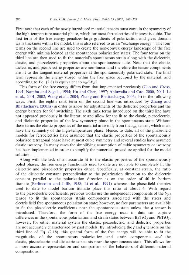
First note that each of the newly introduced material tensors must contain the symmetry ofthe high-temperature material phase, which for most ferroelectrics of interest is cubic. Thefirst term of the free energy penalizes large gradients of polarization and gives domainwalls thickness within the model, this is also referred to as an ‘‘exchange energy’’. The fourterms on the second line are used to create the non-convex energy landscape of the freeenergy with minima located at the spontaneous polarization states. The four terms on thethird line are then used to fit the material’s spontaneous strain along with the dielectric,elastic, and piezoelectric properties about the spontaneous state. Note that the elastic,dielectric, and piezoelectric properties are non-linear, and therefore the tensor componentsare fit to the tangent material properties at the spontaneously polarized state. The finalterm represents the energy stored within the free space occupied by the material, andaccording to Eq. (2.8) is equivalent to k0EiEi/2.This form of the free energy differs from that implemented previously (Cao and Cross,

1991; Nambu and Sagala, 1994; Hu and Chen, 1997; Ahluwalia and Cao, 2000, 2001; Liet al., 2001, 2002; Wang et al., 2004; Zhang and Bhattacharya, 2005a, b) in the followingways. First, the eighth rank term on the second line was introduced by Zhang andBhattacharya (2005a) in order to allow for adjustments of the dielectric properties and theenergy barriers for 901 switching. The sixth rank terms introduced on the third line havenot appeared previously in the literature and allow for the fit to the elastic, piezoelectric,and dielectric properties of the low symmetry phase in the spontaneous state. Withoutthese terms the elastic properties of the material arise only from the cijkl tensor, which musthave the symmetry of the high-temperature phase. Hence, to date, all of the phase-fieldmodels for ferroelectrics have assumed that the elastic properties of the spontaneouslypolarized tetragonal phase have at most cubic symmetry and several studies have assumedelastic isotropy. In many cases the simplifying assumption of cubic symmetry or isotropyhas been implemented in order to simplify the numerical procedure applied for the modelsolution.Along with the lack of an accurate fit to the elastic properties of the spontaneously

poled phases, the free energy functionals used to date are not able to completely fit thedielectric and piezoelectric properties either. Specifically, at constant strain, the ratioof the dielectric constant perpendicular to the polarization direction to the dielectricconstant parallel to the polarization direction is on the order of 40 in bariumtitanate (Berlincourt and Jaffe, 1958; Li et al., 1991) whereas the phase-field theoriesused to date to model barium titanate place this ratio at about 4. With regardto the piezoelectric coefficients, previous works use the independent components of the bijkl

tensor to fit the spontaneous strain components associated with the stress andelectric field free spontaneous polarization state; however, no free parameters are availableto fit the piezoelectric coefficients near the spontaneous state unless the g tensor isintroduced. Therefore, the form of the free energy used to date can capturedifferences in the spontaneous polarization and strain states between BaTiO3 and PbTiO3,however, for either material system the elastic, piezoelectric, and dielectric propertiesare not accurately characterized by past models. By introducing the f and g tensors on thethird line of Eq. (2.18), this general form of the free energy will be able to fit themagnitudes of the spontaneous polarization and strain components and theelastic, piezoelectric and dielectric constants near the spontaneous state. This allows fora more accurate representation and comparison of the behaviors of different materialcompositions.


3. Planar domain wall solutions

In this section the solutions for initially straight domain walls in the y–z plane moving atconstant velocity v in the x-direction are presented. The polarization and any appliedelectric fields will exist in the x–y plane, i.e. Pz ¼ 0 and Ez ¼ 0, and generalized plane strainis assumed, i.e. exz ¼ eyz ¼ 0 and ezz is uniform. Transforming to a coordinate system thatis moving along with the domain wall at constant velocity v, symmetry considerationsdictate that the solutions for stresses, strains, electric fields, electric displacements,polarizations, and micro-forces are functions of x only. Given these constraints,compatibility of strains implied by Eq. (2.4) yield

�yy ¼ c0yþ �0yy. (3.1)

With no free charge q, Maxwell’s laws governing the quasi-static electric displacement andthe electric field distributions, Eqs. (2.5) and (2.7), imply that

dDx

dx¼ 0) Dx ¼ D0

x, (3.2)

dEy

dx¼ 0) Ey ¼ E0

y. (3.3)

The parameters �0yy; D0x; and E0

y are the constant axial strain, electric displacement, andelectric field in the associated directions. The constant c0 arises if the domain wall is curveddue to the deformation. Here only cases where the wall remains straight after thedeformation will be considered and hence c0 is taken to be zero. Then, with the fact thatexx ¼ exx(x) and hence ux,yx ¼ exx,y ¼ 0, the momentum balances from Eq. (2.1), imply

d

dxsxx � rv2�xx

� �¼ 0) sxx ¼ rv2�xx þ s0xx, (3.4)

d

dxsxy � 2rv2�xy

� �¼ 0) sxy ¼ 2rv2�xy þ s0xy, (3.5)

where s0xx and s0xy are constants. Finally, the micro-force balances from Eq. (2.16) become

dxxx

dx� Zx ¼ �vbxx

dPx

dx� vbxy

dPy

dx, (3.6)

dxxy

dx� Zy ¼ �vbyx

dPx

dx� vbyy

dPy

dx. (3.7)

The solutions to Eqs. (3.1)–(3.7) are subject to the boundary conditions sxxð1Þ ¼

sþxx; sxxð�1Þ¼s�xx;sxyð1Þ ¼ sþxy; sxyð�1Þ ¼ s�xy;Dxð1Þ ¼ D0x; Dxð�1Þ ¼ D0

x; Zx(N) ¼ 0,Zx(�N) ¼ 0, Zy(N) ¼ 0, and Zy(�N) ¼ 0. Along with these boundary conditions thegoverning equations can be solved for the electromechanical structure of a planar domainwall moving at constant velocity. Before presenting such results we first derive anexpression for the Eshelby driving traction on a domain wall following the procedure ofFried and Gurtin (1994).

Sharp interface theories of domain wall dynamics require a kinetic law that describes thenormal velocity of points along the interface. Such kinetic laws usually relate the normalvelocity to the jump in the Eshelby energy-momentum tensor across the wall. Thefollowing derivation provides this relationship based on the diffuse interface theory. First,

multiply Eqs. (3.2) and (3.4)–(3.7) by !Ex, exx, 2exy, Px,x, and Py,x respectively. Then,defining the electrical enthalpy h as h " c!EiDi, the sum of these equations can berearranged as follows:

x ! h

! "

$3:8%

d applying theN to N can be

(3.9)

he domain wall

(3.10)

tensor across aon of this resultrical results for

ing at constanthe plane x " 0.pendix and ares a spontaneous-energy domaind electric fields,erface (Shu andbarium titanateplane.wall structures01 domain wall.dditionally, all

ero. For each of!0.329e0, and

ld axial stress is.gnitude of thezoelectric effect.with the valuelso of interest is

(3.11)


d

dxxxxPx;x # xxyPy;x # sxx!xx !

1

2rv2!2xx # 2sxy!xy ! 2rv2!2xy ! ExD

" !v bxxP2x;x # bxy # byx

# $Py;xPx;x # byyP

2y;x

h i.

After defining 1aU& " a$1% ! a$!1% and /aS " [a(N)+a(!N)]/2, anidentity 1abU& " hai1bU& # hbi1aU&, the integral of Eq. (3.8) from x " !shown to yield

f ' 1hU& ! hsxxi1!xxU& ! 2hsxyi1!xyU& # hDxi1ExU& "1

mv,

where the Eshelby driving traction f is defined within Eq. (3.9) and tmobility m is defined as

1

m"

Z 1

!1bxxP

2x;x # bxy # byx

# $Px;xPy;x # byyP

2y;x

h idx.

The left-hand side of Eq. (3.9) is the jump in Eshelby’s energy–momentumflat planar domain wall moving in the x-direction. An additional discussiand its implications will be discussed later in this section. Next, numesolutions to Eqs. (3.1)–(3.7) are presented.The solutions are presented in a Cartesian coordinate system mov

velocity v in the x-direction. The center of the domain wall will occupy tThe material properties used for the simulations are specified in the Aprepresentative of barium titanate. At room temperature barium titanate hapolarization in one of the six /1 0 0S crystallographic directions. The lowwall configurations are those that exist in the absence of far field stresses ani.e. walls that allow for both strain and charge compatibility across the intBhattacharya, 2001). The two low-energy wall types for room temperatureare the 1801 wall on a {1 0 0} plane and the 901 domain wall on a {1 1 0}The first sets of simulations to be presented are for stationary domain

with v " 0. Figs. 1a and b plot the polarization and axial stress near a 18For these simulations the Px, Dx, Ex, Ey, and sxx fields are equal to zero. Aof the shear stresses and the z-components of the electrical fields are also zthe simulations the out-of-plane strain is set to the spontaneous level ezz "the axial strain parallel to the domain wall, !0yy, is set such that the far fies1yy " 0:2; 0; or ! 0:2. The characteristic length scale is l0 "

%%%%%%%%%%%%%%%%%%a0P0=E0

p

Note from Fig. 1a that the application of stress increases the mapolarization far from the domain wall, and this is of course due to the pieAlso notice that the stresses within the domain wall are significant1.5s0 " 1GPa for the model properties used here for barium titanate. Athe domain wall surface energy, which is obtained from

gwall "Z 1

!1c! c$1%( &dx.

ARTICLE IN PRESS

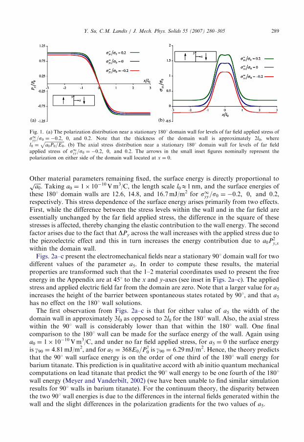
Fig. 1. (a) The polarization distribution near a stationary 1801 domain wall for levels of far field applied stress of

s1yy=s0 ¼ �0:2; 0; and 0:2. Note that the thickness of the domain wall is approximately 2l0, where

l0 ¼ffiffiffiffiffiffiffiffiffiffiffiffiffiffiffiffiffiffia0P0=E0

p. (b) The axial stress distribution near a stationary 1801 domain wall for levels of far field

applied stress of s1yy=s0 ¼ �0:2; 0; and 0:2. The arrows in the small inset figures nominally represent the

polarization on either side of the domain wall located at x ¼ 0.

Y. Su, C.M. Landis / J. Mech. Phys. Solids 55 (2007) 280–305 289

Other material parameters remaining fixed, the surface energy is directly proportional toffiffiffiffiffia0p

. Taking a0 ¼ 1� 10�10 Vm3/C, the length scale l0E1 nm, and the surface energies ofthese 1801 domain walls are 12.6, 14.8, and 16.7mJ/m2 for s1yy=s0 ¼ �0:2; 0; and 0:2;respectively. This stress dependence of the surface energy arises primarily from two effects.First, while the difference between the stress levels within the wall and in the far field areessentially unchanged by the far field applied stress, the difference in the square of thesestresses is affected, thereby changing the elastic contribution to the wall energy. The secondfactor arises due to the fact that DPy across the wall increases with the applied stress due tothe piezoelectric effect and this in turn increases the energy contribution due to a0P2

y;x

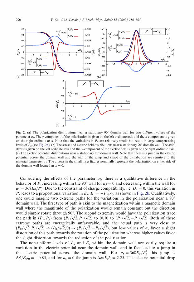
within the domain wall.Figs. 2a–c present the electromechanical fields near a stationary 901 domain wall for two

different values of the parameter a5. In order to compute these results, the materialproperties are transformed such that the 1–2 material coordinates used to present the freeenergy in the Appendix are at 451 to the x and y-axes (see inset in Figs. 2a–c). The appliedstress and applied electric field far from the domain are zero. Note that a larger value for a5increases the height of the barrier between spontaneous states rotated by 901, and that a5has no effect on the 1801 wall solutions.

The first observation from Figs. 2a–c is that for either value of a5 the width of thedomain wall in approximately 3l0 as opposed to 2l0 for the 1801 wall. Also, the axial stresswithin the 901 wall is considerably lower than that within the 1801 wall. One finalcomparison to the 1801 wall can be made for the surface energy of the wall. Again usinga0 ¼ 1� 10�10 Vm3/C, and under no far field applied stress, for a5 ¼ 0 the surface energyis g90 ¼ 4.81mJ/m2, and for a5 ¼ 368E0=P7

0 is g90 ¼ 6.29mJ/m2. Hence, the theory predictsthat the 901 wall surface energy is on the order of one third of the 1801 wall energy forbarium titanate. This prediction is in qualitative accord with ab initio quantum mechanicalcomputations on lead titanate that predict the 901 wall energy to be one fourth of the 1801wall energy (Meyer and Vanderbilt, 2002) (we have been unable to find similar simulationresults for 901 walls in barium titanate). For the continuum theory, the disparity betweenthe two 901 wall energies is due to the differences in the internal fields generated within thewall and the slight differences in the polarization gradients for the two values of a5.

ARTICLE IN PRESS

Fig. 2. (a) The polarization distributions near a stationary 901 domain wall for two different values of the

parameter a5. The y-component of the polarization is given on the left ordinate axis and the x-component is given

on the right ordinate axis. Note that the variations in Px are relatively small, but result in large compensating

levels of Ex (see Fig. 2b). (b) The stress and electric field distributions near a stationary 901 domain wall. The axial

stress is given on the left ordinate axis and the x-component of the electric field is given on the right ordinate axis.

(c) The electric potential distributions near a stationary 901 domain wall. Note that there is a jump in the electric

potential across the domain wall and the sign of the jump and shape of the distribution are sensitive to the

material parameter a5. The arrows in the small inset figures nominally represent the polarization on either side of

the domain wall located at x ¼ 0.

Y. Su, C.M. Landis / J. Mech. Phys. Solids 55 (2007) 280–305290

Considering the effects of the parameter a5, there is a qualitative difference in thebehavior of Px, increasing within the 901 wall for a5 ¼ 0 and decreasing within the wall fora5 ¼ 368E0=P7

0. Due to the constraint of charge compatibility, i.e. Dx ¼ 0, this variation inPx leads to a proportional variation in Ex, Ex ¼ �Px/k0, as shown in Fig. 2b. Qualitatively,one could imagine two extreme paths for the variations in the polarization near a 901domain wall. The first type of path is akin to the magnetization within a magnetic domainwall where the magnitude of the polarization would remain constant but the directionwould simply rotate through 901. The second extremity would have the polarization tracethe path in (Px,Py) from ðP0=

ffiffiffi2p

;P0=ffiffiffi2pÞ to (0, 0) to ðP0=

ffiffiffi2p

;�P0=ffiffiffi2pÞ. Both of these

extreme paths are energetically unfavorable, and the actual path is very close toðP0=

ffiffiffi2p

;P0=ffiffiffi2pÞ ! ðP0=

ffiffiffi2p

; 0Þ ! ðP0=ffiffiffi2p

;�P0=ffiffiffi2pÞ, but low values of a5 favor a slight

distortion of this path towards the rotation of the polarization whereas higher values favorthe slight distortion towards the reduction of the polarization.The non-uniform levels of Px and Ex within the domain wall necessarily require a

variation in the electric potential near the domain wall, and in fact lead to a jump inthe electric potential across the domain wall. For a5 ¼ 368E0=P7

0 this jump isDf/E0l0 ¼ �0.85, and for a5 ¼ 0 the jump is Df/E0l0 ¼ 2.25. This electric potential drop


has been predicted by ab initio computations on lead titanate, Meyer and Vanderbilt(2002), and has a significant effect on the interaction of domain walls with charge defects,Xiao et al. (2005). This feature of the domain wall solutions has interesting consequencesfor sharp interface model of domains which usually assume that the electric potential iscontinuous across a domain wall. These results suggest that the potential drop across thewall should be accounted for within the constitutive response of the wall in a fashionsimilar to that proposed by Gurtin et al. (1998) for mechanical interfaces.

The results to be presented in the following are for steadily propagating domain walls.Here the assumption will be made that the velocities are small with respect to the soundwave speeds in the material such that the inertial terms in Eqs. (3.4) and (3.5) can beneglected. In all cases the axial stress normal to the wall is sxx ¼ 0, the out-of-plane strainis fixed at the spontaneous state ezz ¼ �0.329e0 and the Pz, Dz, Ez, exz, eyz, sxz, and syz

fields are zero. The 901 walls are subjected to simultaneous applied electric field Ey parallelto the domain wall and shear stress sxy with the average axial stress syy ¼ 0 andDx ¼ P0=

ffiffiffi2p

. In the 901 wall case, either Ey or sxy is able to drive the motion of the domainwall in the absence of the other applied field. The 1801 walls are subjected to simultaneousapplied electric field Ey parallel to the domain wall and average axial stress syy. In this casethe application of syy in the absence of Ey does not cause domain wall motion, but syy doesalter the motion in the presence of Ey.

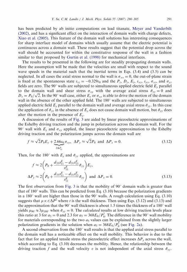
A discussion of the results of Fig. 3 are aided by linear piezoelectric approximations ofthe Eshelby driving traction and the jump in polarization across the domain wall. For the901 wall with Ey and sxy applied, the linear piezoelectric approximation to the Eshelbydriving traction and the polarization jumps across the domain wall are

f �ffiffiffi2p

P0Ey þ 2:66�0|fflffl{zfflffl}2D�0xy

sxy; DPy �ffiffiffi2p

P0 and DPx ¼ 0. (3.12)

Then, for the 1801 with Ey and syy applied, the approximations are

f � 2 P0 þd33sE

11 � d31sE13

sE11

syy

� �Ey,

DPy � 2 P0 þd33sE

11 � d31sE13

sE11

syy

� �and DPx ¼ 0. ð3:13Þ

The first observation from Fig. 3 is that the mobility of 901 domain walls is greater thanthat of 1801 walls. This can be predicted from Eq. (3.10) because the polarization gradientsin a 1801 wall are higher than those in the 901 walls. A rough calculation using Eq. (3.10)suggests that mpt/DP2 where t is the wall thickness. Then using Eqs. (3.12) and (3.13) andthe approximation that the 901 wall thickness is about 1.5 times the thickness of a 1801 wallyields m901E3m1801 when syy ¼ 0. The calculated results at low driving traction levels placethis ratio at 3 for a5 ¼ 0 and 2.3 for a5 ¼ 368E0=P7

0. The difference in the 901 wall mobilityfor materials corresponding to the two a5 values can be explained from the slightly largerpolarization gradients in the solution when a5 ¼ 368E0=P7

0 (see Fig. 2a).A second observation from the 1801 wall results is that the applied axial stress parallel to

the domain wall has a noticeable effect on the wall mobility. This behavior is due to thefact that for an applied tensile stress the piezoelectric effect increases DPy across the wall,which according to Eq. (3.10) decreases the mobility. Hence, the relationship between thedriving traction f and the wall velocity v is not independent of the axial stress syy.

ARTICLE IN PRESS

Fig. 3. Domain wall velocity versus the Eshelby driving traction for a 1801 domain wall under different levels of

applied stress, and for 901 domain walls in materials with different a5 coefficients. For each level of the average

applied stress syy the driving force for the 1801 wall is controlled solely by Ey; however, each of the curves for the

901 walls contain data points from multiple combinations of applied electric field Ey and shear stress sxy.


Effectively, the domain wall mobility decreases as the average axial stress increases. Wenote that a similar behavior occurs for the 901 wall under an applied axial stress, but thiseffect has been omitted here for the sake of clarity on the plots in Fig. 3 and in thisdiscussion. As for the electric potential drop, this feature of the solutions has interestingimplications for sharp interface and other larger scale phenomenological constitutivetheories for domain switching in ferroelectrics. Sharp interface theory Kessler and Balke(2001), single crystal continuum slip theory Huber et al. (1999), and polycrystalline flowtheory Landis (2002b) have each identified the contribution to the driving force forswitching associated with the changes in material properties due to switching. For the caseof 1801 switching these theories predict that a tensile stress will increase the driving forcefor switching when in combination with an electric field as in Eq. (3.13). However, thesetheories usually assume that the domain wall mobility or the critical switching strength is aconstant value. In contrast, the phase-field theory predicts that the domain wall mobility isdecreased by a tensile stress, and in fact this decrease in the mobility is greater, by a factorof 2 when linearized, than the increase in the driving force associated with the changes inthe linear material properties, i.e. f�2EP0ð1þ d33syy=P0Þ but m�1=2bðP0 þ d33syyÞ

2

� ð1� 2d33syy=P0Þ=2bP20.

4. Finite element formulation

The governing equations for the phase-field model include Eqs. (2.1)–(2.9), (2.14), (2.15),and (2.18). When formulating a finite element method to solve these equations the fieldquantities that will be used as nodal degrees of freedom must first be identified. Thesimplest formulation, in terms of the smallest number of degrees of freedom per node,


would implement the components of mechanical displacement from which strain isderived, the components of electrical polarization from which the polarization gradient isderived, and the electrical potential or voltage from which electric field is derived. In orderto implement such a formulation, the constitutive equations must take eij, Pi, Pi,j, and Ei asthe independent variables. However, the Helmholtz free energy has Di instead of Ei as theindependent variable. To address this difficulty, the following Legendre transformation isrequired to derive the electrical enthalpy h:

hð�ij ;Pi;Pi;j ;EiÞ ¼ c� EiDi

¼ 12aijklPi;jPk;l þ

12aijPiPj þ

14¯aijklPiPjPkPl þ

16¯aijklmnPiPjPkPlPmPn

þ 16¯aijklmnrsPiPjPkPlPmPnPrPs þ bijkl�ijPkPl þ

12cijkl�ij�kl

þ f ijklmn�ij�klPmPn þ gijklmn�ijPkPlPmPn �12k0EiEi � EiPi, ð4:1Þ

where the stresses, electric displacements, and micro-forces, xij and Zi, are derived as

sji ¼qh

q�ij

; Di ¼ �qh

qEi

; xji ¼qh

qPi;j; and Zi ¼

qh

qPi

. (4.2)

Then, given Eqs. (2.2), (2.4), (2.7), and (2.15), Eqs. (2.1), (2.3), (2.5), (2.6), and (2.9) can bederived from the following variational statement or principle of virtual work:Z

V

bij_PjdPi dV þ

ZV

r €uidui dV þ

ZV

sjid�ij �DidEi þ ZidPi þ xjidPi;j dV

¼

ZV

bidui � qdfþ gidPi dV þ

ZS

tidui � odfþ xjinjdPi dS. ð4:3Þ

Eq. (4.3) is the foundation for the derivation of the finite element equations for the model.Again, the components of mechanical displacement, electric polarization, and the electricpotential are used as nodal degrees of freedom. The strain, electric field and polarizationgradient are derived within the elements, and finally the stress, electric displacement, andmicro-forces are computed via Eqs. (4.1) and (4.2). We note that even though thepolarization gradient appears in the free energy, C0 continuous elements are in fact suitablefor the solution. This is a fortuitous consequence of Eq. (2.8), given that both electric fieldand polarization can be taken as independent variables. Therefore, the polarizationcomponents take the same status as mechanical displacement and electric potential and thepolarization gradient takes the same status as strain and electric field. If, for example, theelectric field were the order parameter, and both electric potential and components ofelectric field were required as nodal degrees of freedom, then higher order elements wouldbe required in the formulation.

Again, each node in the finite element mesh has mechanical displacement, polarization,and electric potential degrees of freedom. Then, defining the array of degrees of freedom asd, each of the field quantities are interpolated from the nodal quantities with the same setof shape functions such that

ui

f

Pi

8><>:

9>=>; ¼ N½ � df g. (4.4)


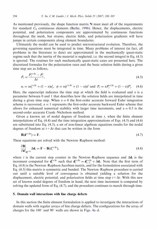
As mentioned previously, the shape function matrix N must meet all of the requirementsfor standard C0 continuous elements (Bathe, 1996). Hence, the displacements, electricpotential, and polarization components are approximated by continuous functionsthroughout the mesh, but strains, electric fields, and polarization gradients will havejumps in certain components along element boundaries.Ultimately the model can be used to predict microstructural evolution. Therefore, the

governing equations must be integrated in time. Many problems of interest (in fact, allproblems in the literature to date) are approximated in the mechanically quasi-staticregime such that the inertia of the material is neglected, i.e. the second integral in Eq. (4.3)is ignored. The routines for such mechanically quasi-static cases are presented here. Thediscretized formulas for the polarization rates and the basic solution fields during a giventime step are as follows,

_Pi ¼PtþDt

i � Pti

Dt, (4.5)

ui ¼ autþDti þ 1� að Þut

i ; f ¼ aftþDtþ 1� að Þft and Pi ¼ aPtþDt

i þ 1� að ÞPti . (4.6)

Here, the superscript indicates the time step at which the field is evaluated and a is aparameter between 0 and 1 that describes how the solution fields are interpolated in timeduring a given time step. When a ¼ 0 the first-order accurate forward Euler integrationscheme is recovered, a ¼ 1 represents the first-order accurate backward Euler scheme thatallows for enhanced numerical stability with larger time increments, and a ¼ 0.5 is thesecond-order accurate Crank–Nicholson method.Given a known set of nodal degrees of freedom at time t, when the finite element

interpolations of Eq. (4.4) and the time integration approximations of Eqs. (4.5) and (4.6)are substituted into Eq. (4.3), a set of non-linear algebraic equations results for the nodaldegrees of freedom at t+Dt that can be written in the form

BðdtþDtÞ ¼ F. (4.7)

These equations are solved with the Newton–Raphson method:

qBqd

��dtþDt

i

Ddi ¼ F� BðdtþDti Þ, (4.8)

where i is the current step counter in the Newton–Raphson sequence and Ddi is theincrement computed for dtþDt

i such that dtþDti ¼ dtþDt

i�1 þ Ddi. Note that the first term ofEq. (4.8) is the Newton–Raphson Jacobian matrix, and for the formulation associated withEq. (4.3) this matrix is symmetric and banded. The Newton–Raphson procedure is carriedout until a suitable level of convergence is obtained yielding a solution for thedisplacement, electric potential, and polarization fields at time step t+Dt. With this newset of known nodal degrees of freedom in hand, the next time increment is computed bysolving the updated form of Eq. (4.7), and the procedure continues to march through time.

5. Domain wall interactions with line charge defects

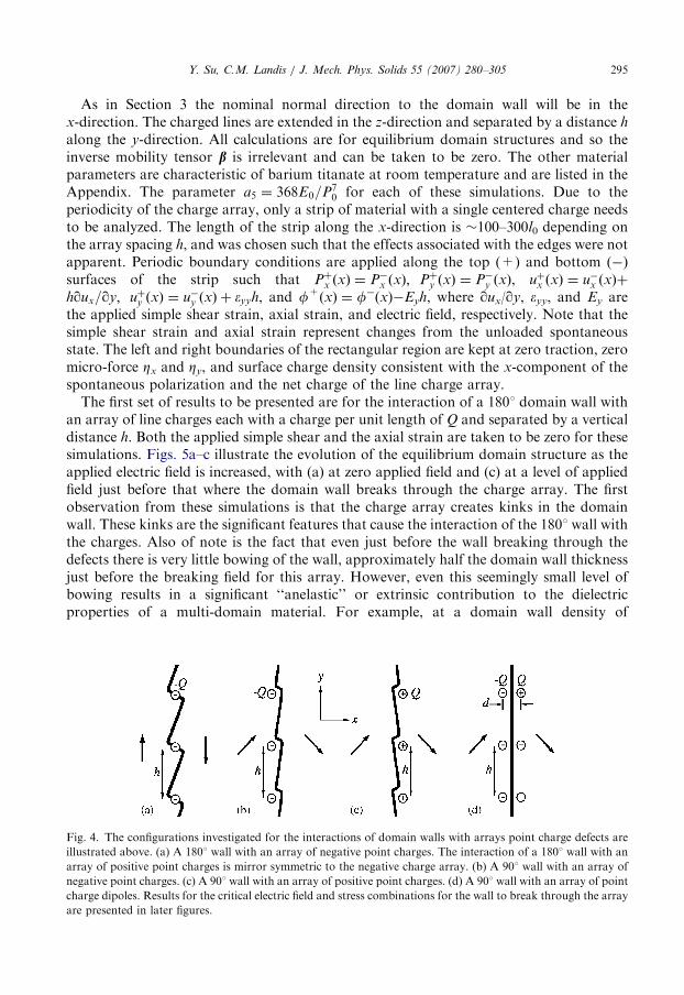
In this section the finite element formulation is applied to investigate the interactions ofdomain walls with regular arrays of line charge defects. The configurations for the array ofcharges for the 1801 and 901 walls are shown in Figs. 4a–d.


As in Section 3 the nominal normal direction to the domain wall will be in thex-direction. The charged lines are extended in the z-direction and separated by a distance h

along the y-direction. All calculations are for equilibrium domain structures and so theinverse mobility tensor b is irrelevant and can be taken to be zero. The other materialparameters are characteristic of barium titanate at room temperature and are listed in theAppendix. The parameter a5 ¼ 368E0=P7

0 for each of these simulations. Due to theperiodicity of the charge array, only a strip of material with a single centered charge needsto be analyzed. The length of the strip along the x-direction is �100–300l0 depending onthe array spacing h, and was chosen such that the effects associated with the edges were notapparent. Periodic boundary conditions are applied along the top (+) and bottom (�)surfaces of the strip such that Pþx ðxÞ ¼ P�x ðxÞ; Pþy ðxÞ ¼ P�y ðxÞ, uþx ðxÞ ¼ u�x ðxÞþ

hqux=qy; uþy ðxÞ ¼ u�y ðxÞ þ �yyh, and f+(x) ¼ f�(x)�Eyh, where qux/qy, eyy, and Ey arethe applied simple shear strain, axial strain, and electric field, respectively. Note that thesimple shear strain and axial strain represent changes from the unloaded spontaneousstate. The left and right boundaries of the rectangular region are kept at zero traction, zeromicro-force Zx and Zy, and surface charge density consistent with the x-component of thespontaneous polarization and the net charge of the line charge array.

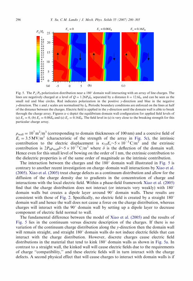
The first set of results to be presented are for the interaction of a 1801 domain wall withan array of line charges each with a charge per unit length of Q and separated by a verticaldistance h. Both the applied simple shear and the axial strain are taken to be zero for thesesimulations. Figs. 5a–c illustrate the evolution of the equilibrium domain structure as theapplied electric field is increased, with (a) at zero applied field and (c) at a level of appliedfield just before that where the domain wall breaks through the charge array. The firstobservation from these simulations is that the charge array creates kinks in the domainwall. These kinks are the significant features that cause the interaction of the 1801 wall withthe charges. Also of note is the fact that even just before the wall breaking through thedefects there is very little bowing of the wall, approximately half the domain wall thicknessjust before the breaking field for this array. However, even this seemingly small level ofbowing results in a significant ‘‘anelastic’’ or extrinsic contribution to the dielectricproperties of a multi-domain material. For example, at a domain wall density of

Fig. 4. The configurations investigated for the interactions of domain walls with arrays point charge defects are

illustrated above. (a) A 1801 wall with an array of negative point charges. The interaction of a 1801 wall with an

array of positive point charges is mirror symmetric to the negative charge array. (b) A 901 wall with an array of

negative point charges. (c) A 901 wall with an array of positive point charges. (d) A 901 wall with an array of point

charge dipoles. Results for the critical electric field and stress combinations for the wall to break through the array

are presented in later figures.

ARTICLE IN PRESS

Fig. 5. The Py/P0 polarization distribution near a 1801 domain wall interacting with an array of line charges. The

lines are negatively charged at a level of Q ¼ 1.26P0l0, separated by a distance h ¼ 12.6l0, and can be seen as the

small red and blue circles. Red indicates polarization in the positive y-direction and blue in the negative

y-direction. The x and y scales are normalized by l0. Periodic boundary conditions are enforced on the lines at half

of the distance between the charges. Electric field is applied in the y-direction until the domain wall is able to break

through the charge array. Figures a–c depict the equilibrium domain wall configuration for applied field levels of

(a) Ey ¼ 0, (b) Ey ¼ 0.08E0 and (c) Ey ¼ 0.16E0. The field level in (c) is very close to the breaking strength for this

particular charge array.


rwall ¼ 107m2/m3 (corresponding to domain thicknesses of 100 nm) and a coercive field ofEc ¼ 3.5MV/m2 (characteristic of the strength of the array in Fig. 5c), the intrinsiccontribution to the electric displacement is k33Ec�5� 10�3 C/m2 and the extrinsiccontribution is 2P0rwalld�5� 10�3 C/m2 where d is the deflection of the domain wall.Hence even for this small level of bowing on the order of 1 nm, the extrinsic contribution tothe dielectric properties is of the same order of magnitude as the intrinsic contribution.The interaction between the charges and the 1801 domain wall illustrated in Fig. 5 is

contrary to another recent investigation on charge–domain wall interactions by Xiao et al.(2005). Xiao et al. (2005) treat charge defects as a continuum distribution and allow for thediffusion of the charge density due to gradients in the concentration of charge andinteractions with the local electric field. Within a phase-field framework Xiao et al. (2005)find that the charge distribution does not interact (or interacts very weakly) with 1801domain walls but creates a dipole layer around 901 domain walls. These results areconsistent with those of Fig. 2. Specifically, no electric field is created by a straight 1801domain wall and hence the wall does not cause a force on the charge distribution, whereascharges will interact with the 901 domain wall by setting up a dipole layer to decreasecomponent of electric field normal to wall.The fundamental difference between the model of Xiao et al. (2005) and the results of

Fig. 5 lies in the continuum versus discrete description of the charges. If there is novariation of the continuum charge distribution along the y-direction then the domain wallwill remain straight, and straight 1801 domain walls do not induce electric fields that caninteract with the charge distribution. However, discrete charges cause electric fielddistributions in the material that tend to kink 1801 domain walls as shown in Fig. 5a. Incontrast to a straight wall, the kinked wall will cause electric fields due to the requirementsof charge ‘‘compatibility,’’ and these electric fields will in turn interact with the chargedefects. A second physical effect that will cause charges to interact with domain walls is if

ARTICLE IN PRESS

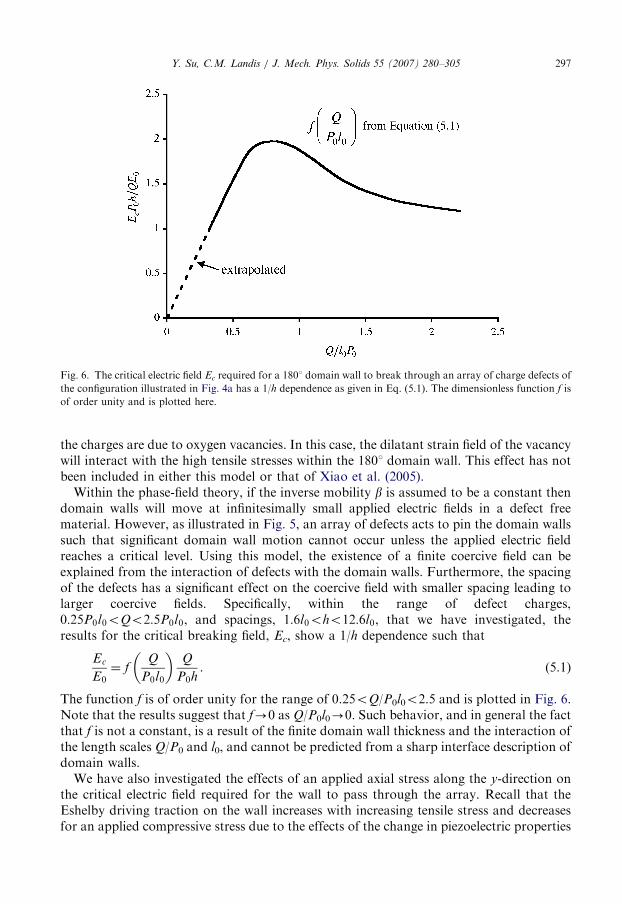
Fig. 6. The critical electric field Ec required for a 1801 domain wall to break through an array of charge defects of

the configuration illustrated in Fig. 4a has a 1/h dependence as given in Eq. (5.1). The dimensionless function f is

of order unity and is plotted here.

Y. Su, C.M. Landis / J. Mech. Phys. Solids 55 (2007) 280–305 297

the charges are due to oxygen vacancies. In this case, the dilatant strain field of the vacancywill interact with the high tensile stresses within the 1801 domain wall. This effect has notbeen included in either this model or that of Xiao et al. (2005).

Within the phase-field theory, if the inverse mobility b is assumed to be a constant thendomain walls will move at infinitesimally small applied electric fields in a defect freematerial. However, as illustrated in Fig. 5, an array of defects acts to pin the domain wallssuch that significant domain wall motion cannot occur unless the applied electric fieldreaches a critical level. Using this model, the existence of a finite coercive field can beexplained from the interaction of defects with the domain walls. Furthermore, the spacingof the defects has a significant effect on the coercive field with smaller spacing leading tolarger coercive fields. Specifically, within the range of defect charges,0:25P0l0oQo2:5P0l0, and spacings, 1:6l0oho12:6l0, that we have investigated, theresults for the critical breaking field, Ec, show a 1/h dependence such that

Ec

E0¼ f

Q

P0l0

� �Q

P0h. (5.1)

The function f is of order unity for the range of 0.25oQ/P0l0o2.5 and is plotted in Fig. 6.Note that the results suggest that f-0 as Q/P0l0-0. Such behavior, and in general the factthat f is not a constant, is a result of the finite domain wall thickness and the interaction ofthe length scales Q/P0 and l0, and cannot be predicted from a sharp interface description ofdomain walls.

We have also investigated the effects of an applied axial stress along the y-direction onthe critical electric field required for the wall to pass through the array. Recall that theEshelby driving traction on the wall increases with increasing tensile stress and decreasesfor an applied compressive stress due to the effects of the change in piezoelectric properties

ARTICLE IN PRESS

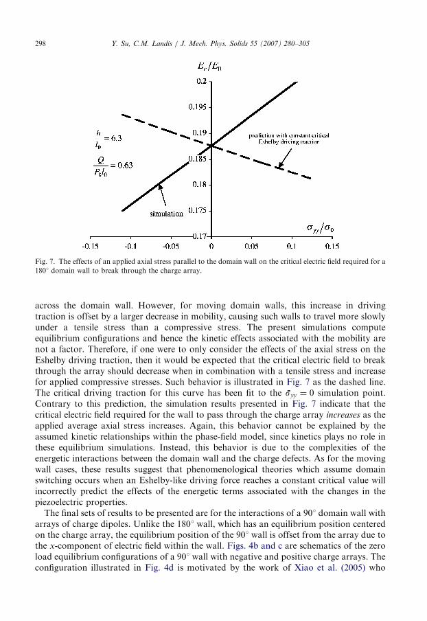
Fig. 7. The effects of an applied axial stress parallel to the domain wall on the critical electric field required for a

1801 domain wall to break through the charge array.


across the domain wall. However, for moving domain walls, this increase in drivingtraction is offset by a larger decrease in mobility, causing such walls to travel more slowlyunder a tensile stress than a compressive stress. The present simulations computeequilibrium configurations and hence the kinetic effects associated with the mobility arenot a factor. Therefore, if one were to only consider the effects of the axial stress on theEshelby driving traction, then it would be expected that the critical electric field to breakthrough the array should decrease when in combination with a tensile stress and increasefor applied compressive stresses. Such behavior is illustrated in Fig. 7 as the dashed line.The critical driving traction for this curve has been fit to the syy ¼ 0 simulation point.Contrary to this prediction, the simulation results presented in Fig. 7 indicate that thecritical electric field required for the wall to pass through the charge array increases as theapplied average axial stress increases. Again, this behavior cannot be explained by theassumed kinetic relationships within the phase-field model, since kinetics plays no role inthese equilibrium simulations. Instead, this behavior is due to the complexities of theenergetic interactions between the domain wall and the charge defects. As for the movingwall cases, these results suggest that phenomenological theories which assume domainswitching occurs when an Eshelby-like driving force reaches a constant critical value willincorrectly predict the effects of the energetic terms associated with the changes in thepiezoelectric properties.The final sets of results to be presented are for the interactions of a 901 domain wall with

arrays of charge dipoles. Unlike the 1801 wall, which has an equilibrium position centeredon the charge array, the equilibrium position of the 901 wall is offset from the array due tothe x-component of electric field within the wall. Figs. 4b and c are schematics of the zeroload equilibrium configurations of a 901 wall with negative and positive charge arrays. Theconfiguration illustrated in Fig. 4d is motivated by the work of Xiao et al. (2005) who


predicted that the interactions of a mobile charge density with domain walls will causeevolution towards a charge dipole layer near 901 domain walls. The applied loadings to thesystem include an electric field parallel to the domain wall Ey ¼ E and a simple shear strainqux/qy applied in order to create a shear stress sxy ¼ t. In all cases the far field axial stresssxx ¼ 0, the far field changes in the axial strains from the initial remanent state are zero,D�yy ¼ 0 and D�zz ¼ 0, and the far field electric displacement in the direction normal to thedomain wall is Dx ¼

ffiffiffi2p

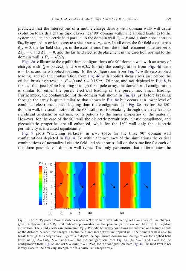
P0.Figs. 8a–c illustrate the equilibrium configurations of a 901 domain wall with an array of

charges with Q ¼ 0.32P0l0 and h ¼ 6.3l0 for (a) the configuration from Fig. 4d withd ¼ 1.6 l0 and zero applied loading, (b) the configuration from Fig. 4c with zero appliedloading, and (c) the configuration from Fig. 4c with applied shear stress just before thecritical breaking stress, i.e. E ¼ 0 and t ¼ 0.159s0. Of note, and not depicted in Fig. 8, isthe fact that just before breaking through the dipole array, the domain wall configurationis similar for either the purely electrical loading or the purely mechanical loading.Furthermore, the configuration of the domain wall shown in Fig. 8a just before breakingthrough the array is quite similar to that shown in Fig. 8c but occurs at a lower level ofcombined electromechanical loading than the configuration of Fig. 8c. As for the 1801domain wall, the small motion of the 901 wall prior to breaking through the array leads tosignificant anelastic or extrinsic contributions to the linear properties of the material.However, for the case of the 901 wall the dielectric permittivity, elastic compliance, andpiezoelectric properties are all enhanced, while for the 1801 wall only the dielectricpermittivity is increased significantly.

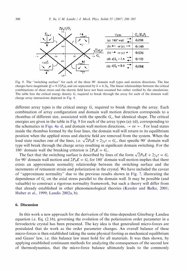
Fig. 9 plots ‘‘switching surfaces’’ in E�t space for the three 901 domain wallconfigurations depicted in Fig. 4. To within the accuracy of the simulations the criticalcombinations of normalized electric field and shear stress fall on the same line for each ofthe three possible 901 domain wall types. The only parameter that differentiates the

Fig. 8. The Py/P0 polarization distribution near a 901 domain wall interacting with an array of line charges,

Q ¼ 0.32P0l0 and h ¼ 6.3l0. Red indicates polarization in the positive y-direction and blue in the negative

y-direction. The x and y scales are normalized by l0. Periodic boundary conditions are enforced on the lines at half

of the distance between the charges. Electric field and shear stress are applied until the domain wall is able to

break through the charge array. Figures a–c depict the equilibrium domain wall configuration for applied field

levels of (a) d ¼ 1.6l0, E ¼ 0 and t ¼ 0 for the configuration from Fig. 4a, (b) E ¼ 0 and t ¼ 0 for the

configuration from Fig. 4c, and (c) E ¼ 0 and t ¼ 0.159s0 for the configuration from Fig. 4c. The load level in (c)

is very close to the breaking strength for this particular charge array.

ARTICLE IN PRESS

Fig. 9. The ‘‘switching surface’’ for each of the three 901 domain wall types and motion directions. The line

charges have magnitude Q ¼ 0.32P0l0 and are separated by h ¼ 6.3l0. The linear relationships between the critical

combinations of shear stress and the electric field have not been assumed but rather verified by the simulations.

The table lists the critical energy density Gc required to break through the array for each of the domain wall/

charge array interactions depicted in Fig. 4.


different array types is the critical energy Gc required to break through the array. Eachcombination of array configuration and domain wall motion direction corresponds to arhombus of different size, associated with the specific Gc, but identical shape. The criticalenergies are given in the table in Fig. 9 for each of the array types (a)–(d), corresponding tothe schematics in Figs. 4a–d, and domain wall motion directions, - or ’. For load statesinside the rhombus formed by the four lines, the domain wall will return to its equilibriumposition when the applied stress and electric field are removed from the system. When theload state reaches one of the lines, i.e.

ffiffiffi2p

P0E þ 2g0t ¼ Gc, that specific 901 domain walltype will break through the charge array resulting in significant domain switching. For the1801 domain wall the breaking criterion is 2P0E ¼ Gc.The fact that the switching surface is described by lines of the form

ffiffiffi2p

P0E þ 2g0t ¼ Gc

for 901 domain wall motion and 2P0E ¼ Gc for 1801 domain wall motion implies that thereexists an approximate normality relationship between the switching surface and theincrements of remanent strain and polarization in the crystal. We have included the caveatof ‘‘approximate normality’’ due to the previous results shown in Fig. 7, illustrating thedependence of Gc on the axial stress parallel to the domain wall. It may be possible (andvaluable) to construct a rigorous normality framework, but such a theory will differ fromthat already established in other phenomenological theories (Kessler and Balke, 2001;Huber et al., 1999; Landis 2002a, b).

6. Discussion

In this work a new approach for the derivation of the time-dependent Ginzburg–Landauequation i.e. Eq. (2.16), governing the evolution of the polarization order parameter in aferroelectric crystal has been presented. The key idea is that generalized micro-forces arepostulated that do work as the order parameter changes. An overall balance of thesemicro-forces is then established taking the same physical footing as mechanical equilibriumand Gauss’ law, i.e. this balance law must hold for all materials. It was then shown, byapplying established continuum methods for analyzing the consequences of the second lawof thermodynamics, that the micro-force balance ultimately leads to the commonly


accepted Ginzburg–Landau evolution equations for the order parameter. The followingquestion can then be posed, have we gained anything by introducing such micro-forces?We would argue that in fact we have. All of reversible, small-deformation, static,mechanics can be established by postulating a strain energy density c(eij) and minimizingthe potential energy of the system subject to the constraints of linear kinematics, i.e.eij ¼ (ui,j+uj,i)/2. Such a procedure leads to the following set of partial differentialequations and boundary conditions,

qcq�ij

� �;j

þ bi ¼ 0 in V andqcq�ij

nj ¼ ti on S. (6.1)

However, Eq. (6.1) is simply a combination of mechanical equilibrium and the constitutivelaw sji ¼ qc/qeij. Hence, by minimizing the potential energy of the system, the physicalcontent of the stresses and their balance (mechanical equilibrium) is obscured. Therefore,we take the view that within the phase-field setting Eq. (2.9) has the same fundamentalphysical priority as Eqs. (2.1)–(2.8). A second rationale for postulating the micro-forces isthat in the presence of other dissipative mechanisms like conductive heat transfer or thediffusion of species within the material, the micro-force balance can be applied within thesecond law of thermodynamics using the systematic approach established by Coleman andNoll (1963) to determine the constraints on the constitutive dependencies.

Within the phase-field framework it is appropriate to consider the domain walls as a setof internal boundary layers that move through the material. The domain wall thicknesslength scale associated with these ‘‘boundary layers’’ is l0 ¼

ffiffiffiffiffiffiffiffiffiffiffiffiffiffiffiffiffiffia0P0=E0

p. Unlike sharp

interface theories that require a specification of the surface energy of the interfaces, thephase-field theory predicts the energy content of the different domain wall types. Thissurface energy is dependent both on the exchange energy parameter a0, and on the featuresof the free energy landscape. For a given free energy functional, the domain wall surfaceenergies are proportional to

ffiffiffiffiffia0p

. Note that simulation results generated by manipulating(i.e. increasing) a0 for the purpose of computational convenience must be interpretedcarefully since such a procedure changes the surface energy of the domain walls. Whensimulating the qualitative response of ferroelectric crystals, increasing a0 for computationalexpediency is likely to yield reasonable behavior. However, for quantitative predictions ofdomain structures and the interactions of domain walls with defects, a more accuraterepresentation of the surface energy is required. Given the disparate length scalesassociated with the domain wall thickness �l0 and the domain structure size �100–1000l0,accurate numerical solutions to large-scale domain structure evolution problems willrequire computational schemes that allow for adaptive mesh refinement (Provotas et al.,1998).

As for the derivation of the governing equations, the finite element formulationpresented here is also a departure from several of the prior studies on phase-field modelingof ferroelectrics that have applied spectral methods for the numerical solutions. Onebenefit of the finite element formulation is the ability to apply any arbitrary form for thematerial free energy that includes the general anisotropy for elastic and piezoelectricproperties. The finite element method also allows for the analysis of arbitrary geometrieswith very general non-periodic or periodic boundary conditions. Examples where suchflexibility is useful include the analysis of domain wall interactions with point or linedefects, like those presented in Section 5, or investigations of domain switching and


nucleation near crack tips by applying asymptotic crack tip boundary conditions in the farfield and the appropriate electromechanical boundary conditions on the crack faces(Landis, 2004). Finally, when solutions for the electric fields in all of free space arerequired, e.g. domain patterns near free surfaces, then more sophisticated boundaryconditions like the Dirichlet to Neumann (DtN) map can be added to the finite elementmethod (Givoli and Keller, 1989) to solve such problems.The methods presented here, including both the introduction of micro-forces and their

balance, and the finite element formulation, can be generalized for the analysis of a widerange of ferroic materials, including shape memory alloys, ferromagnetic materials,magneto-electric materials (BiFeO3), and ferromagnetic shape memory alloys. Of course,in these cases the order parameter is not necessarily the material polarization and thedetails of the physical behavior will also differ. For example, in ferromagnetic materials theorder parameter will be the magnetization, and, in contrast to electrical polarization, themagnetization will rotate its direction without reducing in magnitude. These differencescharacterize the specific details of the physical behavior, but the concepts associated withthe diffuse interface description of domain walls, micro-forces and their balance, and thenumerical techniques can be applied universally to this broad class of materials.

Acknowledgments

The authors would like to acknowledge support from the Office of Naval Research Grantno. N00014-03-1-0537. Special thanks to Johannes Rodel for pointing out the effect of smalllevels of domain wall bowing on the extrinsic dielectric, elastic and piezoelectric properties.

Appendix

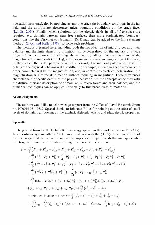
The general form for the Helmholtz free energy applied in this work is given in Eq. (2.18).In a coordinate system with the Cartesian axes aligned with the /1 0 0S directions, a form ofthe free energy that can be used to mimic the properties of single crystals that undergo a cubicto tetragonal phase transformation through the Curie temperature is

c ¼a0

2P21;1 þ P2

2;2 þ P23;3 þ P2

1;2 þ P22;1 þ P2

1;3 þ P23;1 þ P2

2;3 þ P23;2

þ

a1

2P21 þ P2

2 þ P23

� �þ

a2

4P41 þ P4

2 þ P43

� �þ

a3

2P21P2

2 þ P22P2

3 þ P21P

23

� �þ

a4

6P61 þ P6

2 þ P63

� �þ a6 P4

1ðP22 þ P2

3Þ þ P42ðP

21 þ P2

3Þ þ P43ðP

21 þ P2

2Þ� �

þa5

4P41P

42 þ P4

2P43 þ P4

1P43

� ��

b

21�11P2

1 þ �22P22 þ �33P

23

� �

�b2

2ð�22 þ �33ÞP

21 þ ð�11 þ �33ÞP

22 þ ð�11 þ �22ÞP

23

� �b3 ð�12 þ �21ÞP1P2ð

þð�13 þ �31ÞP1P3 þ ð�23 þ �32ÞP2P3Þ þc1

2�211 þ �

222 þ �

233

� �þ c2 �11�22 þ �11�33 þ �22�33ð Þ þ

c3

2�212 þ �

221 þ �

213 þ �

231 þ �

223 þ �

232

� �þ

f 1

2�211 þ

f 2

2ð�222 þ �

233Þ

�þ f 3ð�11�22 þ �11�33Þ þ f 4�22�33 þ

f 5

2ð�212 þ �

221 þ �

213 þ �

231Þ

!f 62"!223 ! !232#

!P21 !

f 12!222 !

f 22"!211 ! !233# ! f 3"!11!22 ! !22!33#

"

!f 4!11!33 !f 52"!212 ! !221 ! !223 ! !232# !

f 62"!213 ! !231#

!P22

measured by Lis polarization in

perties given in

' 10$12 m2=N,

10$12 m2=N,

10$12 C=N,

,

in k!11 & 1980k0ve are calculatedefficients of the

30;

!0P0;

0;

0=!20P0;

!20P0;

=!20P30;


0

!f 12!233 !

f 22"!211 ! !222# ! f 3"!11!33 ! !22!33# ! f 4!11!22

"

!f 52"!213 ! !231 ! !223 ! !232# !

f 62"!212 ! !221#

!P23

!g14!11 !

g24"!22 ! !33#

# $P41 !

g14!22 !

g24"!11 ! !33#

# $P42

!g14!33 !

g24"!11 ! !22#

# $P43 !

g34

!12 ! !21" # P1P32 ! P2P

31

% &

!g34

!13 ! !31" # P1P33 ! P3P

31

% &!

g34

!23 ! !32" # P2P33 ! P3P

32

% &

!1

2k0"D1 $ P1#2 ! "D2 $ P2#2 ! "D3 $ P3#2% &

.

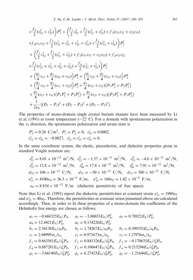
The properties of mono-domain single crystal barium titanate have beenet al. (1991) at room temperature (%22 1C). For a domain with spontaneouthe x3 direction, the spontaneous polarization and strain state is

Ps3 & 0:26 C=m2; Ps

1 & Ps2 & 0; !s33 & 0:0082,

!s11 & !s22 & $0:0027; !s12 & !s13 & !s23 & 0.

In the same coordinate system, the elastic, piezoelectric, and dielectric prostandard Voight notation are:

sE11 & 8:01' 10$12 m2=N; sE12 & $1:57' 10$12 m2=N; sE13 & $4:6

sE33 & 12:8' 10$12 m2=N; sE44 & 17:8' 10$12 m2=N; sE66 & 7:91'

d33 & 106' 10$12 C=N; d31 & $50' 10$12 C=N; d15 & 580'

ks11 & 4100k0 & 36:3' 10$9 F=m; ks33 & 160k0 & 1:42' 10$9 F=m

k0 & 8:854' 10$12 F=m "dielectric permittivity of free space#.

Note that Li et al. (1991) report the dielectric permittivities at constant straand k!33 & 48k0. Therefore, the permittivities at constant stress presented aboaccordingly. Then, in order to fit these properties of a mono-domain the coHelmholtz free energy are chosen as follows:

a1 & $0:668325E0=P0; a2 & $3:80653E0=P30; a3 & 0:78922E0=P

a4 & 12:4421E0=P50; a6 & 0:134226E0=P5

0;

b1 & 2:54138E0=!0P0; b2 & 1:74267E0=!0P0; b3 & 0:399353E0=

c1 & 2:04999!0=s0; c2 & 0:971673!0=s0; c3 & 1:27976!0=sf 1 & 0:663581E0=!20P0; f 2 & 0:841326E0=!20P0; f 3 & $0:170635E

f 4 & 0:687281E0=!20P0; f 5 & 0:106647E0=!20P0; f 6 & 0:213294E0=

g1 & $3:66149E0=!20P30; g2 & 6:27423E0=!20P

30; g3 & $1:21644E0

! "0 0 ! "0 0 ! "0


where P0 ¼ 0.26C/m2, e0 ¼ 0.0082, E0 ¼ 2.18247� 107V/m, and s0 ¼ E0P0/e0 ¼ 692�106N/m2. The definitions of P0 and e0 obviously arise from the spontaneous state. Thecritical electric field E0 is the magnitude of the electric field required to cause homogeneous1801 switching when the electric field is applied in the opposite direction of the uniformspontaneous polarization. Finally, the stress s0 is simply a derived quantity used fornormalizations.The tetragonal elastic properties alone do not uniquely determine the c and f coefficients.

Hence, the c’s have been fit to the cubic elastic properties of the paraelectric phase ofbarium titanate as measured at 150 1C by Berlincourt and Jaffe (1958). We have alsoselected values for a1 and a3 to be in agreement to those reported by Pertsev et al. (1998) asthese parameters primarily affect the characteristics of the energy wells.Note that the coefficients a0 and a5 do not affect the fitting of the coefficients to the

measured material properties. The parameter a5 has been discussed in detail by Zhang andBhattacharya (2005a), and it primarily affects the energy barrier along a line connectingadjacent energy wells in polarization space. In this work a5 has been chosen to be eitherzero or 368E0=P7

0. The coefficient a0 is important in determining the domain wall thicknessand domain wall surface energy. For a0 ¼ 1� 10�10 Vm3/C the theory predicts 1801domain walls on the order of 2 nm thick with a surface energy of approximately 15mJ/m2.

References

Ahluwalia, R., Cao, W., 2000. Influence of dipolar defects on switching behavior in ferroelectrics. Phys. Rev. B 63,

012103–012114.

Ahluwalia, R., Cao, W., 2001. Size dependence of domain patterns in a constrained ferroelectric system. J. Appl.

Phys. 89, 8105–8109.

Allik, H., Hughes, T.J.R., 1970. Finite element method for piezoelectric vibration. Int. J. Numer. Methods Eng. 2,

151–157.

Bathe, K.J., 1996. Finite Element Procedures. Prentice-Hall, New Jersey.

Berlincourt, D., Jaffe, H., 1958. Elastic and piezoelectric coefficients of single-crystal barium titanate. Phys. Rev.

111, 143–148.

Cao, W., Cross, L.E., 1991. Theory of tetragonal twin structures in ferroelectric perovskites with a first-order

phase transition. Phys. Rev. B 44, 5–12.

Cohen, R.E., Krakauer, H., 1992. Electronic structure studies of differences in ferroelectric behavior of BaTiO3

and PbTiO3. Ferroelectrics 136, 65–83.

Coleman, R.D., Noll, W., 1963. The thermodynamics of elastic materials with heat conduction and viscosity.

Arch. Rational Mech. Anal. 13, 167–178.

Devonshire, A.F., 1954. Theory of ferroelectrics. Philos. Mag. Suppl. 3, 85.

Fried, E., Gurtin, M.E., 1993. Continuum theory of thermally induced phase transitions based on an order

parameter. Physica D 68, 326–343.

Fried, E., Gurtin, M.E., 1994. Dynamic solid–solid transitions with phase characterized by an order parameter.

Physica D 72, 287–308.

Givoli, D., Keller, J.B., 1989. A finite-element method for large domains. Comp. Methods Appl. Mech. Eng. 76,

41–66.

Gurtin, M.E., 1996. Generalized Ginzburg–Landau and Cahn–Hilliard equations based on a microforce balance.

Physica D 92, 178–192.

Gurtin, M.E., Weissmuller, J., Larche, F., 1998. A general theory for curved deformable interfaces in solids at

equilibrium. Philos. Mag. A 78, 1093–1109.

Hu, H.L., Chen, L.Q., 1997. Computer simulation of 90 degree ferroelectric domain formation in two-dimensions.

Mater. Sci. Eng. A 238, 182–191.

Huber, J.E., Fleck, N.A., Landis, C.M., McMeeking, R.M., 1999. A constitutive model for ferroelectric

polycrystals. J. Mech. Phys. Solids 47, 1663–1697.

Jona, F., Shirane, G., 1962. Ferroelectric Crystals. Pergamon Press, New York.


Kessler, H., Balke, H., 2001. On the local and average energy release in polarization switching phenomena.

J. Mech. Phys. Solids 49, 953–978.

Landis, C.M., 2002a. A new finite-element formulation for electromechanical boundary value problems. Int.

J. Numer. Methods Eng. 55, 613–628.

Landis, C.M., 2002b. Fully coupled, multi-axial, symmetric constitutive laws for polycrystalline ferroelectric

ceramics. J. Mech. Phys. Solids 50, 127–152.

Landis, C.M., 2004. Energetically consistent boundary conditions for electromechanical fracture. Int. J. Solids

Struct. 41, 6291–6315.

Li, Y.L., Hu, S.Y., Liu, Z.K., Chen, L.Q., 2001. Phase-field model of domain structures in ferroelectric thin films.

Appl. Phys. Lett. 78, 3878–3880.

Li, Y.L., Hu, S.Y., Liu, Z.K., Chen, L.Q., 2002. Effect of substrate constraint on the stability and evolution of

ferroelectric domain structures in thin films. Acta Mater. 50, 395–411.

Li, Z., Chan, S.K., Grimsditch, M.H., Zouboulis, E.S., 1991. The elastic and electromechanical properties of

tetragonal BaTiO3 single crystals. J. Appl. Phys. 70, 7327–7332.

McMeeking, R.M., Landis, C.M., 2005. Electrostatic forces and stored energy for deformable dielectric materials.

J. Appl. Mech. 72, 581–590.

Meyer, B., Vanderbilt, D., 2002. Ab initio study of ferroelectric domain walls in PbTiO3. Phys. Rev. B 65, 104111.

Nambu, S., Sagala, D.A., 1994. Domain formation and elastic long-range interaction in ferroelectric perovskites.

Phys. Rev. B 50, 5838–5847.

Nye, J.F., 1957. Physical Properties of Crystals. Oxford University Press, Great Britain.

Pertsev, N.A., Zembilgotov, A.G., Tagantsev, A.K., 1998. Effect of mechanical boundary conditions on phase

diagrams of epitaxial ferroelectric thin films. Phys. Rev. Lett. 80, 1988–1991.

Provotas, N., Goldenfeld, N., Dantzig, J., 1998. Efficient computation of dendritic microstructures using adaptive

mesh refinement. Phys. Rev. Lett. 80, 3308–3311.

Shu, Y.C., Bhattacharya, K., 2001. Domain patterns and macroscopic behaviour of ferroelectric materials. Philos.

Mag. B 81, 2021–2054.

Toupin, R.A., 1956. The elastic dielectric. J. Rational Mech. Anal. 5, 849–914.

Wang, J., Landis, C.M., 2004. On the fracture toughness of ferroelectric ceramics with electric field applied

parallel to the crack front. Acta Mater. 52, 3435–3446.

Wang, J., Shi, S.Q., Chen, L.Q., Li, Y., Zhang, T.Y., 2004. Phase field simulations of ferroelectric/ferroelastic

polarization switching. Acta Mater. 52, 749–764.

Warren, W.L., Dimos, D., Tuttle, B.A., Nasby, R.D., Pike, G.E., 1994. Electronic domain pinning in Pb(Zr,Ti)O3

thin films and its role in fatigue. Appl. Phys. Lett. 65, 1018–1020.

Xiao, Y., Shenoy, V.B., Bhattacharya, K., 2005. Depletion layers and domain walls in semiconducting

ferroelectric thin films. Phys. Rev. Lett. 95, 247603.

Xu, F., Trolier-McKinstry, S., Ren, W., Xu, B., Xie, Z.-L., Hemker, K.J., 2005. Domain wall motion and its

contribution to the dielectric and piezoelectric properties of lead zirconate titanate films. J. Appl. Phys. 89,

1336–1348.

Zhang, W., Bhattacharya, K., 2005a. A computational model of ferroelectric domains. Part I: model formulation

and domain switching. Acta Mater. 53, 185–198.

Zhang, W., Bhattacharya, K., 2005b. A computational model of ferroelectric domains. Part II: grain boundaries

and defect pinning. Acta Mater. 53, 199–209.

Documents

Continuum thermodynamics of ferroelectric domain …landis/Landis/Research_files/JMPS2007.pdfContinuum thermodynamics of ferroelectric domain evolution: Theory, ﬁnite element