Embed Size (px)
Citation preview

Continuum Modeling and Simulation.
Rodolfo R. Rosales, Adam Powell, FranzJosef Ulm, Kenneth Beers
MIT, Spring 2006

1 Continuum Modeling and Simulation. MIT, FebruaryMarch, 2006.

Contents
1 Introduction 51.1 Scope and Purpose of This Document . . . . . . . . . . . . . . . . . . . . . . . . . . 51.2 Lecture Outline . . . . . . . . . . . . . . . . . . . . . . . . . . . . . . . . . . . . . . 51.3 List of Symbols . . . . . . . . . . . . . . . . . . . . . . . . . . . . . . . . . . . . . . 6
2 Conservation Laws in Continuum Modeling 72.1 Introduction. . . . . . . . . . . . . . . . . . . . . . . . . . . . . . . . . . . . . . . . 72.2 Continuum Approximation; Densities and Fluxes. . . . . . . . . . . . . . . . . . . . 8
2.2.1 Examples . . . . . . . . . . . . . . . . . . . . . . . . . . . . . . . . . . . . . 82.3 Conservation Laws in Mathematical Form. . . . . . . . . . . . . . . . . . . . . . . . 10
Integral Form of a Conservation Law (1D case) . . . . . . . . . . . . . . . . . . . . 11Differential Form of a Conservation Law (1D case) . . . . . . . . . . . . . . . . . . 11Shock Waves . . . . . . . . . . . . . . . . . . . . . . . . . . . . . . . . . . . . . . . 11Integral Form of a Conservation Law (multiD case) . . . . . . . . . . . . . . . . . . 12Differential Form of a Conservation Law (multiD case) . . . . . . . . . . . . . . . . 12Differential Form of the Equations for Vector Conservation Laws . . . . . . . . . . . 13
2.4 Phenomenological Equation Closure. . . . . . . . . . . . . . . . . . . . . . . . . . . 132.4.1 Examples . . . . . . . . . . . . . . . . . . . . . . . . . . . . . . . . . . . . . 14
Example: River Flow . . . . . . . . . . . . . . . . . . . . . . . . . . . . . . . . 14— Quasiequilibrium approximation . . . . . . . . . . . . . . . . . . . . . . . . . 14Example: Traffic Flow . . . . . . . . . . . . . . . . . . . . . . . . . . . . . . . 15Example: Heat Conduction . . . . . . . . . . . . . . . . . . . . . . . . . . . . . 15— Fick’s Law . . . . . . . . . . . . . . . . . . . . . . . . . . . . . . . . . . . . . 16— Thermal conductivity, diffusivity, heat equation . . . . . . . . . . . . . . . . 16Example: Granular Flow . . . . . . . . . . . . . . . . . . . . . . . . . . . . . . 17Example: Inviscid Fluid Flow . . . . . . . . . . . . . . . . . . . . . . . . . . . 18— Incompressible Euler Equations . . . . . . . . . . . . . . . . . . . . . . . . . 18— Incompressible NavierStokes Equations . . . . . . . . . . . . . . . . . . . . 18— Gas Dynamics . . . . . . . . . . . . . . . . . . . . . . . . . . . . . . . . . . . 19— Equation of State . . . . . . . . . . . . . . . . . . . . . . . . . . . . . . . . 19— Isentropic Euler Equations of Gas Dynamics . . . . . . . . . . . . . . . . . . 19— NavierStokes Equations for Gas Dynamics . . . . . . . . . . . . . . . . . . 19
2.5 Concluding Remarks. . . . . . . . . . . . . . . . . . . . . . . . . . . . . . . . . . . . 19
2

Continuum Modeling and Simulation. MIT, FebruaryMarch, 2006. 3
3 Timestepping Algorithms and the Enthalpy Method 203.1 Introduction . . . . . . . . . . . . . . . . . . . . . . . . . . . . . . . . . . . . . . . . 203.2 Finite Differences and the Energy Equation . . . . . . . . . . . . . . . . . . . . . . 20
3.2.1 Explicit time stepping . . . . . . . . . . . . . . . . . . . . . . . . . . . . . . 213.2.2 Implicit Timestepping . . . . . . . . . . . . . . . . . . . . . . . . . . . . . . 233.2.3 SemiImplicit Time Integration . . . . . . . . . . . . . . . . . . . . . . . . . 243.2.4 AdamsBashforth . . . . . . . . . . . . . . . . . . . . . . . . . . . . . . . . . 243.2.5 AdamsMoulton . . . . . . . . . . . . . . . . . . . . . . . . . . . . . . . . . . 253.2.6 RungeKutta Integration . . . . . . . . . . . . . . . . . . . . . . . . . . . . . 25
3.3 Enthalpy Method . . . . . . . . . . . . . . . . . . . . . . . . . . . . . . . . . . . . . 253.4 Finite Volume Approach to Boundary Conditions . . . . . . . . . . . . . . . . . . . 26
4 Weighted Residual Approach to Finite Elements 284.1 Finite Element Discretization . . . . . . . . . . . . . . . . . . . . . . . . . . . . . . 28
4.1.1 Galerkin Approach to Finite Elements . . . . . . . . . . . . . . . . . . . . . 294.2 Green’s Functions and Boundary Elements . . . . . . . . . . . . . . . . . . . . . . . 304.3 Fourier Series Methods . . . . . . . . . . . . . . . . . . . . . . . . . . . . . . . . . . 31
5 Linear Elasticity 325.1 From Heat Diffusion to Elasticity Problems . . . . . . . . . . . . . . . . . . . . . . . 32
5.1.1 1D Heat Diffusion – 1D Elasticity Analogy . . . . . . . . . . . . . . . . . . 325.1.2 3D Extension . . . . . . . . . . . . . . . . . . . . . . . . . . . . . . . . . . . 34
5.2 The Theorem of Virtual Work . . . . . . . . . . . . . . . . . . . . . . . . . . . . . . 365.2.1 From the Theorem of Virtual Work in 1D to Finite Element Formulation . . 365.2.2 Theorem of Minimum Potential Energy in 3D Linear Isotropic Elasticity . . 405.2.3 3D Finite Element Implementation . . . . . . . . . . . . . . . . . . . . . . . 425.2.4 Homework Set: Water Filling of a Gravity Dam . . . . . . . . . . . . . . . . 42
5.3 Concluding Remarks . . . . . . . . . . . . . . . . . . . . . . . . . . . . . . . . . . . 46
6 Discrete to Continuum Modeling 486.1 Introduction. . . . . . . . . . . . . . . . . . . . . . . . . . . . . . . . . . . . . . . . 486.2 Wave Equations from MassSpring Systems. . . . . . . . . . . . . . . . . . . . . . . 49
Longitudinal Motion . . . . . . . . . . . . . . . . . . . . . . . . . . . . . . . . . 49Nonlinear Elastic Wave Equation (for a Rod) . . . . . . . . . . . . . . . . . . . 51Example: Uniform Case . . . . . . . . . . . . . . . . . . . . . . . . . . . . . . . 51— Sound Speed . . . . . . . . . . . . . . . . . . . . . . . . . . . . . . . . . . . 51Example: Small Disturbances . . . . . . . . . . . . . . . . . . . . . . . . . . . 51— Linear Wave Equation, and Solutions . . . . . . . . . . . . . . . . . . . . . 51Fast Vibrations . . . . . . . . . . . . . . . . . . . . . . . . . . . . . . . . . . . 51— Dispersion . . . . . . . . . . . . . . . . . . . . . . . . . . . . . . . . . . . . 52— Long Wave Limit . . . . . . . . . . . . . . . . . . . . . . . . . . . . . . . . . 52Transversal Motion . . . . . . . . . . . . . . . . . . . . . . . . . . . . . . . . . . 53Stability of the Equilibrium Solutions . . . . . . . . . . . . . . . . . . . . . . . 53Nonlinear Elastic Wave Equation (for a String) . . . . . . . . . . . . . . . . . . 54Example: Uniform String with Small Disturbances . . . . . . . . . . . . . . . . 54— Uniform String Nonlinear Wave Equation. . . . . . . . . . . . . . . . . . . . 54
Continuum Modeling and Simulation. MIT, FebruaryMarch, 2006. 4
— Linear Wave Equation. . . . . . . . . . . . . . . . . . . . . . . . . . . . . . 54— Stability and Laplace’s Equation. . . . . . . . . . . . . . . . . . . . . . . . . 54— Illposed Time Evolution. . . . . . . . . . . . . . . . . . . . . . . . . . . . . 54General Motion: Strings and Rods . . . . . . . . . . . . . . . . . . . . . . . . . . 54
6.3 Torsion Coupled Pendulums: SineGordon Equation. . . . . . . . . . . . . . . . . . 55Hooke’s Law for Torsional Forces . . . . . . . . . . . . . . . . . . . . . . . . . 55Equations for N torsion coupled equal pendulums . . . . . . . . . . . . . . . . 56Continuum Limit . . . . . . . . . . . . . . . . . . . . . . . . . . . . . . . . . . . 57— SineGordon Equation . . . . . . . . . . . . . . . . . . . . . . . . . . . . . . . 57— Boundary Conditions . . . . . . . . . . . . . . . . . . . . . . . . . . . . . . 57Kinks and Breathers for the Sine Gordon Equation . . . . . . . . . . . . . . . . . 58Example: Kink and AntiKink Solutions . . . . . . . . . . . . . . . . . . . . . 58Example: Breather Solutions . . . . . . . . . . . . . . . . . . . . . . . . . . . . 59Pseudospectral Numerical Method for the SineGordon Equation . . . . . . . . . 60
6.4 Suggested problems. . . . . . . . . . . . . . . . . . . . . . . . . . . . . . . . . . . . 61
Chapter 1
Introduction
1.1 Scope and Purpose of This Document
This document serves as lecture notes for the Continuum Modeling and Simulation set of lectures in Introduction to Modeling and SImulation, Spring, 2006. As with the lectures themselves, this is authored by the six faculty members who teach the twelve lectures in this set. As such, the length, style, and notation may differ slightly from lecturer to lecturer. This document therefore serves not only to provide all of the material in one place, but also to help us to unify the notation schemes as much as possible in order to smooth the transitions as much as possible.
1.2 Lecture Outline
Lectures in this series, and chapters in this document, are summarized as follows:
1. February 15–17: Rodolfo Rosales. These lectures will introduce the continuum approximations which roughly describe physical systems at a coarse scale, such as density and displacement fields, and also introduce conservation laws as a framework for continuum modeling. Diffusion and heat conduction will be the motivating examples for this section.
2. February 21–27: Adam Powell. The treatment of heat conduction will expand in two ways: first discussing methods for time integration of the transient heat conduction equation, and second introducing the enthalpy method for incorporating phase changes into heat conduction simulations. These lectures will also include a brief introduction to the weighed residual approach to the finite element method.
3. March 1–March 6: FranzJosef Ulm. This section will introduce the variational approach to finite elements for solid mechanics. It will focus on the statics of a gravity dam, illustrating the oneelement solution and accuracy as more elements are introduced.
4. March 8–March 13: Kenneth Beers. Moving to fluids, this section will discuss the complications inherent to discretizing the NavierStokes equations for incompressible fluid flow, including spurious modes in the pressure field and artificial diffusion due to the convective terms, and present methods for resolving these problems.
5
Continuum Modeling and Simulation. MIT, FebruaryMarch, 2006. 6
5. March 15, 20: Raul Radovitzky. This section will demonstrate a hybrid Lagrangian and Eulerian approach for modeling fullycoupled interactions between continuum fluids and solids, often referred to as FluidStructure Interactions.
6. March 17: Rodolfo Rosales. Rosales returns to discuss the relationship between discrete and continuum behavior, focusing on longitudinal and transverse waves and torsioncoupled pendulums.
This document covers the lectures of Rosales, Powell and Ulm, including the final Rosales lecture.
1.3 List of Symbols
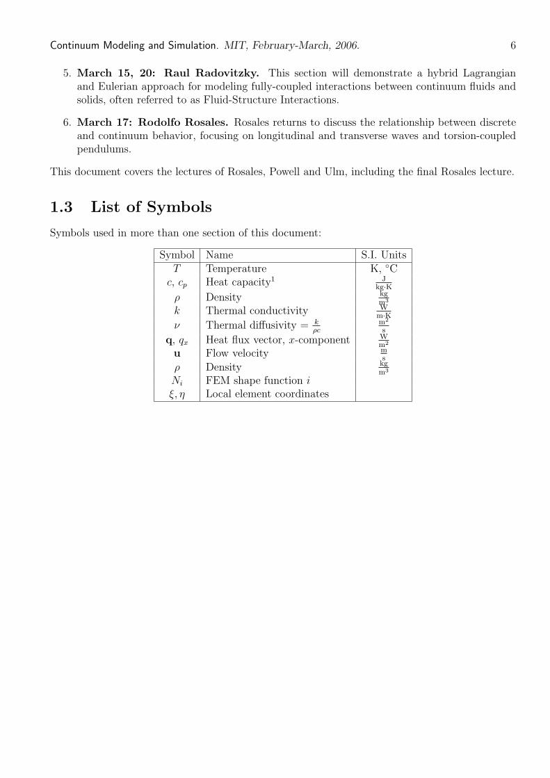
Symbols used in more than one section of this document:
Symbol T c, cp
ρ k ν
q, qx
u ρ Ni
ξ, η
Name S.I. Units Temperature K, ◦C
JHeat capacity1 kg·K kgDensity 3mWThermal conductivity
m·K 2k mThermal diffusivity =
ρc s WHeat flux vector, xcomponent 2mmFlow velocity s kgDensity 3m
FEM shape function i Local element coordinates
Chapter 2
Conservation Laws in Continuum Modeling
These notes give examples illustrating how conservation principles are used to obtain (phenomenological) continuum models for physical phenomena. The general principles are presented, with examples from traffic flow, river flows, heat conduction, granular flows, gas dynamics and diffusion.
2.1 Introduction. In formulating a mathematical model for a continuum physical system, there are three basic steps that are often used:
A. Identify appropriate conservation laws (e.g. mass, momentum, energy, etc) and their corresponding densities and fluxes.
B. Write the corresponding equations using conservation.
C. Close the system of equations by proposing appropriate relationships between the fluxes and the densities.
Of these steps, the mathematical one is the second. While it involves some subtlety, once you understand it, its application is fairly mechanical. The first and third steps involve physical issues, and (generally) the third one is the hardest one, where all the main difficulties appear in developing a new model. In what follows we will go through these steps, using some practical examples to illustrate the ideas.
Of course, once a model is formulated, a fourth step arises, which is that of analyzing and validating the model, comparing its predictions with observations ... and correcting it whenever needed. This involves simultaneous mathematical and physical thinking. You should never forget that a model is no better than the approximations (explicit and/or implicit) made when deriving it. It is never a question of just “solving” the equations, forgetting what is behind them.
7
Continuum Modeling and Simulation. MIT, FebruaryMarch, 2006. 8
2.2 Continuum Approximation; Densities and Fluxes. The modeling of physical variables as if they were a continuum field is almost always an approximation. For example, for a gas one often talks about the density ρ, or the flow velocity u, and thinks of them as functions of space and time: ρ = ρ(x, t) or u = u(x, t). But the fact is that a gas is made up by very many discrete molecules, and the concepts of density, or flow velocity, only make sense as local averages. These averages must be made over scales large enough that the discreteness of the gas becomes irrelevant, but small enough that the notion of these local averages varying in space and time makes sense.
Thus, in any continuum modeling there are several scales. On the one hand one has the “visible” scales, which are the ones over which the mathematical variables in the model vary (densities, fluxes). On the other hand, there are the “invisible” scales, that pertain to the microscales that have been averaged in obtaining the model. The second set of scales must be much smaller than the first set for the model to be valid. Unfortunately, this is not always the case, and whenever this fails all sort of very interesting (and largely open) problems in modern science and engineering arise.
Note that the reason people insist on trying to use continuum type models, even in situations where one runs into the difficulties mentioned at the end of the last paragraph, is that continuum models are often much simpler (both mathematically and computationally) than anything else, and supply general understanding that is often very valuable.
The first step in the modeling process is to identify conserved quantities (e.g. mass) and define the appropriate densities and fluxes — as in the following examples.
2.2.1 Examples
Example 2.2.1 River Flow (a one dimensional example).
Consider a nice river (or a channel) flowing down a plain (e.g. the Mississippi, the Nile, etc.). Let x be the length coordinate along the river, and at every point (and time) along the river let A = A(x, t) be the filled (by water) crosssection of the river bed.
We note now that A is the volume density (volume per unit length) of water along the river. We 1also note that, since water is incompressible, volume is conserved. Finally, let Q = Q(x, t) be
the volume flux of water down the river (i.e.: volume per unit time). Notice that, if u = u(x, t) is
the average flow velocity down the river, then Q = uA (by definition of u).
Thus, in this case, an appropriate conservation law is the conservation of volume, with corresponding density A and flux Q. We note that both A and Q are regularly measured at various points along important rivers.
Example 2.2.2 Traffic Flow (a one dimensional example).
Consider a one lane road, in a situation where there are no crossroads (e.g.: a tunnel, such as the Lincoln tunnel in NYC, or the Summer tunnel in Boston). Let x be length along the road. Under “heavy” traffic conditions,2 we can introduce the notions of traffic density ρ = ρ(x, t) (cars per
1We are neglecting here such things as evaporation, seepage into the ground, etc. This cannot always be done. 2Why must we assume “heavy” traffic?

Continuum Modeling and Simulation. MIT, FebruaryMarch, 2006. 9
unit length) and traffic flow q = q(x, t) (cars per unit time). Again, we have q = uρ, where u is the average car flow velocity down the road.
In this case, the appropriate conservation law is, obviously, the conservation of cars. Notice that this is one example where the continuum approximation is rather borderline (since, for example, the local averaging distances are almost never much larger than a few car separation lengths). Nevertheless, as we will see, one can gain some very interesting insights from the model we will develop (and some useful practical facts).
Example 2.2.3 Heat Conduction.
Consider the thermal energy in a chunk of solid material (such as, say, a piece of copper). Then the thermal energy density (thermal energy per unit volume) is given by U = c T (x, t), where T is the temperature, c is the specific heat per unit mass, and ρ is the density of the material (for simplicity we will assume here that both c and ρ are constant). The thermal energy flow, q = q(x, t) is now a vector, whose magnitude gives the energy flow across a unit area normal to the flow direction.
In this case, assuming that heat is not being lost or gained from other energy forms, the relevant conservation law is the conservation of heat energy.
Example 2.2.4 Steady State (dry) Granular Flow.
Consider steady state (dry) granular flow down some container (e.g. a silo, containing some dry granular material, with a hole at the bottom). At every point we characterize the flow in terms of two velocities: an horizontal (vector) velocity u = u(x, y, z, t), and a vertical (scalar) velocity v = v(x, y, z, t), where x and y are the horizontal length coordinates, and z is the vertical one.
The mass flow rate is then given by Q = ρ [u, v], where ρ is the mass density — which we will assume is nearly constant. The relevant conservation is now the conservation of mass.
This example is different from the others in that we are looking at a steady state situation. We also note that this is another example where the continuum approximation is quite often “borderline”, since the scale separation between the grain scales and the flow scales is not that great.
Example 2.2.5 Inviscid Fluid Flow.
For a fluid flowing in some region of space, we consider now two conservation laws: conservation of mass and conservation of linear momentum. Let now ρ = ρ(x, t), u = u(x, t) and p = p(x, t) be, respectively, the fluid density, flow velocity, and pressure — where we use either [u, v, w] or [u1, u2, u3] to denote the components of u, and either [x, y, z] or [x1, x2, x3] to denote the components of x. Then:
• The mass conservation law density is . . . . . . . . . . . . . . . . . . . . . . . . . . . . . . . . . . . . . . . . . . . . . . . . . . ρ. The mass conservation law flow is . . . . . . . . . . . . . . . . . . . . . . . . . . . . . . . . . . . . . . . . . . . . . . . . . . . . ρu.•
• The linear momentum conservation law density is . . . . . . . . . . . . . . . . . . . . . . . . . . . . . . . . . . ρu. • The linear momentum conservation law flow is . . . . . . . . . . . . . . . . . . . . . . . . . . . . ρu ⊗ u + p I.
The first two expressions above are fairly obvious, but the last two (in particular, the last one) require some explanation. First of all, momentum is a vector quantity. Thus its conservation is
Continuum Modeling and Simulation. MIT, FebruaryMarch, 2006. 10
equivalent to three conservation laws, with a vector density and a rank two tensor3 flow (we explain this below). Second, momentum can be transferred from one part of a liquid to another in two ways: Advection: as a parcel of fluid moves, it carries with it some momentum. Let us consider this mechanism component by component: The momentum density component ρ ui is advected with a flow rate ρ ui u = ρ [uiu1, uiu2, uiu3]. Putting all three components together, we get for the momentum flux (due to advection) the expression ρ [ui uj] = ρu ⊗ u — i.e., a rank two tensor, where each row (freeze the first index) corresponds to the flux for one of the momentum components. Forces: momentum is transferred by the forces exerted by one parcel of fluid on another. If we assume that the fluid is inviscid, then these forces can only be normal, and are given by the pressure (this is, actually, the “definition” of inviscid). Thus, again, let us consider this mechanism component by component: the momentum transfer by the pressure in the direction given by the unit vector4 ei = [δi j], corresponding to the density ρ ui, is the force per unit area (normal to ei) by the fluid. Thus the corresponding momentum flow vector is p ei. Putting all three components together, we get for the momentum flux (due to pressure forces) the expression p [δi j] = p I — again a rank two tensor, now a scalar multiple of the identity rank two tensor I.
Regarding the zero viscosity (inviscid) assumption: Fluids can also exert tangential forces, which also affect the momentum transfer. Momentum can also be transferred in the normal direction by diffusion of “faster” molecules into a region with “slower” molecules, and vice versa. Both these effects are characterized by the viscosity coefficient — which here we assume can be neglected.
Note that in some of the examples we have given only one conservation law, and in others two (further examples, with three or more conservation laws invoked, exist). The reason will become clear when we go to the third step (step C in section 2.1). In fact, steps A and C in section 2.1 are intimately linked, as we will soon see.
2.3 Conservation Laws in Mathematical Form. In this section we assume that we have identified some conservation law, with conserved density ρ = ρ(x, t), and flux F = F(x, t), and derive mathematical formulations for the conservation hypothesis. In other words, we will just state in mathematical terms the fact that ρ is the density for a conserved quantity, with flux F.
First consider the one dimensional case (where the flux F is a scalar, and there is only one space coordinate: x). In this case, consider some (fixed) arbitrary interval in the line Ω = {a ≤ x ≤ b}, and let us look at the evolution in time of the conserved quantity inside this interval. At any given time, the total amount of conserved stuff in Ω is given by (this by definition of density) � b
M(t) = ρ(x, t) dx . (3.1) a
Further, the net rate at which the conserved quantity enters Ω is given by (definition of flux)
R(t) = F (a, t)− F (b, t) . (3.2) 3If you do not know what a tensor is, just think of it as a vector with more than one index (the rank is the number
of indexes). This is all you need to know to understand what follows. 4Here δi j is the Kronecker delta, equal to 1 if i = j, and to 0 if i =� j.
11 Continuum Modeling and Simulation. MIT, FebruaryMarch, 2006.
It is also possible to have sources and sinks for the conserved quantity. 5 In this case let s = s(x, t) be the total net amount of the conserved quantity, per unit time and unit length,
provided by the sources and sinks. For the interval Ω we have then a net rate of added conserved stuff, per unit time, given by � b
S(t) = s(x, t) dx . (3.3) a
The conservation law can now be stated in the mathematical form
d dt M = R + S , (3.4)
Ω.which must apply for any choice of interval Since this equation involves only integrals of Integral Form of the Conservation Law. the relevant densities and fluxes, it is known as the
Assume now that the densities and fluxes are nice enough to have nice derivatives. Then we can write: � b � bd ∂ ∂
dtM =
∂tρ(x, t) dx and R = −
∂xF (x, t) dx . (3.5)
a a
Equation (3.4) can then be rewritten in the form � b � � ∂ ∂ ρ(x, t) + F (x, t)− s(x, t) dx = 0 , (3.6)
∂t ∂x a
which must apply for any choice of the interval Ω. It follows that the integrand above in (3.6) must vanish identically. This then yields the following partial differential equation involving the density, flux and source terms:
∂ ∂ ρ(x, t) + F (x, t) = s(x, t) . (3.7)
∂t ∂x
This equation is known as the Differential Form of the Conservation Law.
Remark 2.3.1 You may wonder why we even bother to give a name to the form of the equations in (3.4), since the differential form in (3.7) appears so much more convenient to deal with (it is just one equation, not an equation for every possible choice of Ω). The reason is that it is not always possible to assume that the densities and fluxes have nice derivatives. Oftentimes the physical systems involved develop, as they evolve,6 short enough scales that force the introduction of discontinuities into the densities and fluxes — and then (3.7) no longer applies, but (3.4) still does. Shock waves are the best known example of this situation. Examples of shock waves you may be familiar with are: the sonic boom produced by a supersonic aircraft; the hydraulic jump occurring near the bottom of the discharge ramp in a large dam; the wavefront associated with a flood moving down a river; the backward facing front of a traffic jam; etc. Some shock waves can cause quite spectacular effects, such as those produced by supernova explosions.
5As an illustration, in the inviscid fluid flow case of example 2.2.5, the effects of gravity translate into a vertical source of momentum, of strength ρ g per unit volume — where g is the acceleration of gravity. Other body forces have similar effects.
6Even when starting with very nice initial conditions.

�
�
�
� �
� � �
12 Continuum Modeling and Simulation. MIT, FebruaryMarch, 2006.
Now let us consider the multidimensional case, when the flux F is a vector. In this case, consider some (fixed but arbitrary) region in space Ω, with boundary ∂Ω, and inside unit normal along the boundary n̂. We will now look at the evolution in time of the conserved quantity inside this region. At any given time, the total amount of conserved stuff in Ω is given by
M(t) = ρ(x, t) dV . (3.8) Ω
On the other hand, the net rate at which the conserved quantity enters Ω is given by
R(t) = F(x, t) · n dS . (3.9) ˆ∂Ω
Let also s = s(x, t) be the total net amount of conserved quantity, per unit time and unit volume, provided by any sources and/or sinks. For the region Ω we have then a net rate of added conserved stuff, per unit time, given by
S(t) = s(x, t) dV . (3.10) Ω
The conservation law can now be stated in the mathematical form (compare with equation (3.4)) — Integral Form of the Conservation Law:
d M = R + S , (3.11)
dt
which must apply for any choice of the region Ω.
If the densities and fluxes are nice enough to have nice derivatives, we can write:
d ∂ M = ρ(x, t) dV and R = −
Ω div(F(x, t)) dV , (3.12)
dt Ω ∂t
where we have used the Gauss divergence theorem for the second integral. Equation (3.11) can then be rewritten in the form
∂ ρ(x, t) + div(F(x, t))− s(x, t) dV = 0 , (3.13)
∂t Ω
which must apply for any choice of the region Ω. It follows that the integrand above in (3.13) must vanish identically. This then yields the following partial differential equation involving the density, flux and source terms (compare with equation (3.7))
∂ ρ(x, t) + div(F(x, t)) = s(x, t) . (3.14)
∂t
This equation is known as the Differential Form of the Conservation Law.
Remark 2.3.2 In the case of a vector conservation law, the density ρ and the source term s will both be vectors, while the flux F will be a rank two tensor (each row being the flux for the corresponding element in the density vector ρ). In this case equation (3.14) is valid component by

� �
Continuum Modeling and Simulation. MIT, FebruaryMarch, 2006. 13
component, but can be given a vector meaning if we define the divergence for a rank two tensor F = [Fi j] as follows: � ∂
div(F) = Fi j ,∂xjj
so that div(F) is a vector (each element corresponding to a row in F). You should check that this is correct.7
2.4 Phenomenological Equation Closure. From the results in section 2.3 it is clear that each conservation principle can be used to yield an evolution equation relating the corresponding density and flux. However, this is not enough to provide a complete system of equations, since each conservation law provides only one equation, but requires two (in principle) “independent” variables. Thus extra relations between the fluxes and the densities must be found to be able to formulate a complete mathematical model. This is the Closure Problem, and it often requires making further assumptions and approximations about the physical processes involved.
Closure is actually the hardest and the subtler part of any model formulation. How good a model is, typically depends on how well one can do this part. Oftentimes the physical processes considered are very complex, and no good understanding of them exist. In these cases one is often forced to make “brute force” phenomenological approximations (some formula — with a few free parameters — relating the fluxes to the densities is proposed, and then it is fitted to direct measurements). Sometimes this works reasonably well, but just as often it does not (producing situations with very many different empirical fits, each working under some situations and not at all in others, with no clear way of knowing “a priori” if a particular fit will work for any given case).
We will illustrate how one goes about resolving the closure problem using the examples introduced earlier in subsection 2.2.1. These examples are all “simple”, in the sense that one can get away with algebraic formulas relating the fluxes with the densities. However, this is not the only possibility, and situations where extra differential equations must be introduced also arise. The more complex the process being modeled is, the worse the problem, and the harder it is to close the system (with very many challenging problems still not satisfactorily resolved).
An important point to be made is that the formulation of an adequate mathematical model is only the beginning. As the examples below will illustrate, it is often the case that the mathematical models obtained are quite complicated (reflecting the fact that the phenomena being modeled are complex), and often poorly understood. Thus, even in cases where accurate mathematical models have been known for well over a century (as in classical fluids), there are plenty of open problems still around ... and even now new, unexpected, behaviors are being discovered in experimental laboratories. The fact is that, for these complex phenomena, mathematics alone is not enough. There is just too much that can happen, and the equations are too complicated to have explicit solutions. The only possibility of advance is by a simultaneous approach incorporating experiments and observations, numerical calculations, and theory. � ∂7Recall that, for a vector field, div(v) =
∂xj vj .
j

Continuum Modeling and Simulation. MIT, FebruaryMarch, 2006. 14
2.4.1 Examples
Example 2.4.1 River Flow (see example 2.2.1).
In this case we can write the conservation equation
At +Qx = 0 , (4.1)
where A and Q were introduced in example 2.2.1, and we ignore any sources or sinks for the water in the river. In order to close the model, we now claim that it is reasonable to assume that Q
is a function of A; that is to say Q = Q(A, x) — for a uniform, manmade channel, one has
Q = Q(A). We justify this hypothesis as follows:
First: For a given river bed shape, when the flow is steady (i.e.: no changes in time) the average flow velocity u follows from the balance between the force of gravity pulling the water down the slope, and the friction force on the river bed. This balance depends only on the river bed shape, its slope, and how much water there is (i.e. A). Thus, under these conditions, we have u = u(A, x). Consequently Q = Q(A, x) = u(A, x)A.
Second: As long as the flow in the river does not deviate too much from steady state (“slow” changes), the we can assume that the relationship Q = Q(A, x) that applies for steady flow remains (approximately) valid. This is the quasiequilibrium approximation, which is often invoked in problems like this. How well it works in any given situation depends on how fast the processes leading to the equilibrium situation (the one that leads to Q = Q(A, x)) work — relative to the time scales of the river flow variations one is interested in. For actual rivers and channels, it turns out that this approximation is good enough for many applications.
Of course, the actual functional relationship Q = Q(A, x) (to be used to model a specific river) cannot be calculated theoretically, and must be extracted from actual measurements of the river flow under various conditions. The data is then fitted by (relatively simple) empirical formulas, with free parameters selected for the best possible match.
However, it is possible to get a qualitative idea of roughly how Q depends on A, by the following simple argument: The force pulling the water downstream (gravity) is proportional to the slope of the bed, the acceleration of gravity, the density of water, and the volume of water. Thus, roughly speaking, this force has the form Fg ≈ cg A (where cg = cg (x) is some function). On the other hand, the force opposing this motion, in the simplest possible model, can be thought as being proportional to the wetted perimeter of the river bed (roughly P ∝
√A) times the frictional force on
the bed (roughly proportional to the velocity u). That is Ff ≈ cf u √A, for some friction coefficient
cf . These two forces must balance (Fg = Ff ), leading to u ≈ cu
√A (where cu = cg /cf ), thus:
Q ≈ cu A3/2 . (4.2)
Of course, this is too simple for a real river. But the feature of the flux increasing faster than linear
is generally true — so that Q as a function of A produces a concave graph, with dQ/dA > 0
and d2Q/dA2 > 0.
15 Continuum Modeling and Simulation. MIT, FebruaryMarch, 2006.
Example 2.4.2 Traffic Flow (see example 2.2.2).
In this case we can write the conservation equation
ρt + qx = 0 , (4.3)
where ρ and q were introduced in example 2.2.2, and we ignore any sources or sinks for cars (from road exit and incoming ramps, say). Just as in the river model, we close now the equations by
claiming that it is reasonable to assume that q is a function of ρ, that is to say q = q(ρ, x) — for
a nice, uniform, road, one has q = q(ρ). Again, we use a quasiequilibrium approximation to
justify this hypothesis:
Under steady traffic conditions, it is reasonable to assume that the drivers will adjust their car speed to the local density (drive faster if there are few cars, slower if there are many). This yields u = u(ρ, x), thus q = u(ρ, x)ρ = q(ρ, x). Then, if the traffic conditions do not vary too rapidly, we can assume that the equilibrium relationship q = q(ρ, x) will still be (approximately) valid — quasiequilibrium approximation.
As in the river flow case, the actual functional dependence to be used for a given road must follow from empirical data. Such a fit for the Lincoln tunnel in NYC is given by8
q = a ρ log(ρj /ρ) , (4.4)
where a = 17.2 mph, and ρj = 228 vpm (vehicles per mile). The generic shape of this formula is always true: q is a convex function of ρ, reaching a maximum flow rate qm for some value ρ = ρm, and then decreases back to zero flow at a jamming density ρ = ρj . In particular, dq/dρ is
a decreasing function of ρ, with d2q/dρ2 < 0.
For the formula above in (4.4), we have: ρm = 83 vpm and qm = 1430 vph (vehicles per hour), with a corresponding flow speed um = qm/ρm = a. The very existence of ρm teaches us a rather useful fact, even before we solve any equation: in order to maximize the flow in a highway, we should try to keep the car density near the optimal value ρm. This is what the lights at the entrances to freeways attempt to do during rush hour. Unfortunately, they do not work very well for this purpose, as some analysis with the model above (or just plain observation of an actual freeway) will show. In this example the continuum approximation is rather borderline. Nevertheless, the equations have the right qualitative (and even rough quantitative) behavior, and are rather useful to understand many features of how heavy traffic behaves.
Example 2.4.3 Heat Conductivity (see example 2.2.3).
In this case we can write the conservation equation
ρ c Tt + div(q) = s , (4.5)
where ρ c, T and q were introduced in example 2.2.3, and s = s(x, t) is the heat supplied (per unit volume and unit time) by any sources (or sinks) — e.g. electrical currents, chemical reactions, etc.
8Greenberg, H., 1959. An analysis of traffic flow. Oper. Res. 7:79–85.

16 Continuum Modeling and Simulation. MIT, FebruaryMarch, 2006.
We now complete the model by observing that heat flows from hot to cold, and postulating that the heat flow across a temperature jump is proportional to the temperature difference (this can be checked experimentally, and happens to be an accurate approximation). This leads to Fick’s Law for the heat flow:
q = −k�T , (4.6)
where k is the coefficient of thermal conductivity of the material.9 For simplicity we will assume here that c, ρ and k are constant — though this is not necessarily true in general.
Substituting (4.6) into (4.5), we then obtain the heat or diffusion equation:
Tt = ν�2T + f , (4.7)
k swhere ν = is the thermal diffusivity of the material, and f = .
ρc ρc
In deriving the equation above, we assumed that the heat was contained in a chunk of solid material. The reason for this is that, in a fluid, heat can also be transported by motion of the fluid (convection). In this case (4.6) above must be modified to:
q = −k�T + ρ c T u , (4.8)
where u = u(x, t) is the fluid velocity. Then, instead of (4.7), we obtain
Tt + div(uT ) = ν�2T + f . (4.9)
In fact, this is the simplest possible situation that can occur in a fluid. The reason is that, generally, the fluid density depends on temperature, so that the fluid motion ends up coupled to the temperature variations, due to buoyancy forces. Then equation (4.9) must be augmented with the fluid equations, to determine u and the other relevant fluid variables — see example 2.4.5.
Remark 2.4.1 Note that ν has dimensions Length2
. Thus, given a length L, a time scale is Time
provided by τ = L2/ν. Roughly speaking, this is the amount of time it would take to heat (or cool) a region of size L by diffusion alone. If you go and check the value of ν for (say) water, you will find out that it would take a rather long time to heat even a cup of tea by diffusion alone (you should do this calculation). The other term in (4.9) is crucial in speeding things up.
Remark 2.4.2 If the fluid is incompressible, then div(u) = 0 (see example 2.4.5), and equation (4.9) takes the form
Tt + (u · �)T = ν�2T + f . (4.10)
Note that the left hand side in this equation is just the time derivative of the temperature in a fixed parcel of fluid, as it is being carried around by the flow.
Remark 2.4.3 Equations such as (4.9) and (4.10) are satisfied not just by the temperature, but by many other quantities that propagate by diffusion (i.e.: their fluxes satisfy Fick’s Law (4.6)). Examples are given by any chemicals in solution in a liquid (salt, sugar, colorants, pollutants, etc.). Of course, if there are any reactions these chemicals participate in, these reactions will have to be incorporated into the equations (as sources and sinks).
9k must be measured experimentally, and varies from material to material.

17 Continuum Modeling and Simulation. MIT, FebruaryMarch, 2006.
Example 2.4.4 Steady State (dry) Granular Flow (see example 2.2.4).
In this case we can write the conservation equation
div(Q) = 0 , (4.11)
where Q = ρ[u, v] is as in example 2.2.4, and there are no time derivatives involved because we assumed that the density ρ was nearly constant (we also assume that there are no sources or sinks for the media). These equation involves three unknowns (the three flow velocities), so we need some extra relations between them to close the equation.
The argument now is as follows: as the grain particles flow down (because of the force of gravity), they will also — more or less randomly — move to the sides (due to particle collisions). We claim now that, on the average, it is easier for a particle to move from a region of low vertical velocity to one of high vertical velocity than the reverse.10 The simplest way to model this idea is to propose that the horizontal flow velocity u is proportional to the horizontal gradient of the vertical flow velocity v. Thus we propose a law of the form:
u = b�⊥v (4.12)
where b is a coefficient (having length dimensions) and �⊥ denotes the gradient with respect to the horizontal coordinates x and y. Two important points:
A. Set the coordinate system so that the z axis points down. Thus v is positive when the flow is downwards, and b above is positive.
B. Equation (4.12) is a purely empirical proposal, based on some rough intuition and experimental observations. However, it works. The predictions of the resulting model in equation (4.13) below have been checked against laboratory experiments, and they match the observations, provided that the value of b is adjusted properly (typically, b must be taken around a few particle diameters).
Substituting (4.12) into (4.11), using the formula for the divergence, and eliminating the common constant factor ρ, we obtain the following model equation for the vertical velocity v:
0 = vz + b�2 v = vz + b (vxx + vyy ) . (4.13) ⊥
Note that this is a diffusion equation, except that the role of time has been taken over by the vertical coordinate z. Mathematical analysis of this equation shows that it only makes sense to solve it for z decreasing; i.e.: from bottom to top in the container where the flow takes place. This, actually, makes perfect physical sense: if you have a container full of (say) dry sand, and you open a hole at the bottom, the motion will propagate upwards through the media. On the other hand, if you move the grains at the top, the ones at the bottom will remain undisturbed. In other words, information about motion in the media propagates upward, not downwards.
10Intuitively: where the flow speed is higher, there is more space between particles where a new particle can move into.
18 Continuum Modeling and Simulation. MIT, FebruaryMarch, 2006.
Example 2.4.5 Inviscid Fluid Flow (see example 2.2.5). In this case, using the densities and fluxes introduced in example 2.2.5, we can write the conservation equations:
ρt + div(ρu) = 0 (4.14) for the conservation of mass, and
(ρu)t + div(ρu ⊗ u) +�p = F (4.15)
for the conservation of momentum. Here F = F(x, t) denotes the body forces11 (which are momentum sources), and we have used the mathematical identity (you should check this) div(p I) = �p. Another easy to check mathematical identity is div(u ⊗m) = (div(m))u + (m · �)u. Using this second identity, with m = ρu, in equation (4.15), and substituting from equation (4.14) to eliminate the term containing the divergence of m, we obtain:
ρ (ut + (� · u)u) +�p = F . (4.16)
The problem now is that we have four equations and five unknowns (density, pressure and the three velocities). An extra equation is needed. Various possibilities exist, and we illustrate a few below.
Incompressibility Assumption (liquids). Liquids are generally very had to compress. This means that, as a parcel of fluid is carried around by the flow, its volume (equivalently, its density) will change very little. If we then make the assumption that the liquid density does not change at all (due to pressure changes ... it certainly may change due to temperature changes, or solutes12 in the liquid), then we obtain the following additional equation:
ρt + (� · u) ρ = 0 . (4.17)
This equation simply states that the time derivative of the density, following a parcel of fluid as it moves, vanishes. In other words: the fluid is incompressible (though it need not have a constant
⎫⎬ ⎭
density). In this case we can write a complete system of equations for the fluid motion. Namely:
0 = ρt + (� · u) ρ , div(u) ,0 (4.18) =
F = ρ (ut + (� · u)u) +�p , where the second equation follows from (4.14), upon use of (4.17). These are known as the Incompressible Euler Equations for a fluid. The “simplest” situation arises when ρ can be assumed constant, and then the first equation above is not needed. However, even in this case, the behavior of the solutions to these equations is not well understood — and extremely rich.
Remark 2.4.4 The equations above ignore viscous effects, important in modeling many physical situations. Viscosity is incorporated with the method used in example 2.4.3, by adding to the momentum flux components proportional to derivatives of the flow velocity u. What results from this are the Incompressible NavierStokes Equations.
Furthermore, heat conduction effects can also be considered (and are needed to correctly model many physical situations). This requires the introduction of a new independent variable into the equations (temperature), and the use of one more conservation law (energy).
11Such as gravity.12For example, salt.

19 Continuum Modeling and Simulation. MIT, FebruaryMarch, 2006.
Gas Dynamics.For gases one cannot assume incompressibility. In this case, one must introduce another conservation law (conservation of energy), and yet another variable: the internal energy per unit mass e. This results in five equations (conservation of mass (4.14), conservation of momentum (4.15), and conservation of energy) and six variables (density ρ, flow velocity u, pressure p and internal energy e). At this stage thermodynamics comes to the rescue, providing an extra relationship: the equation of state. For example, for an ideal gas with constant specific heats (polytropic gas) one has:
p e = cv T and p = RρT = Equation of state: e = , (4.19) ⇒
(γ − 1) ρ
where cv is the specific heat at constant volume, cp is the specific heat at constant pressure, R = cp − cv is the gas constant and γ = cp/cv is the ratio of specific heats.
A simplifying assumption that can be made, applicable in some cases, is that the flow is isentropic.13
In this case the pressure is a function of the density only, and (4.14) and (4.15) then form a complete system: the Isentropic Euler Equations of Gas Dynamics. For a polytropic gas:
p = κ ργ , (4.20)
where κ is a constant. In one dimension the equations are
ρt + (ρ u)x = 0 and (ρ u)t + (ρ u 2 + p)x = 0 , (4.21)
where p = p(ρ).
Remark 2.4.5 The closure problem in this last example involving gas dynamics seemed rather simple, and (apparently) we did not have to call upon any “quasiequilibrium” approximation, or similar. However, this is so only because we invoked an already existing (mayor) theory: thermodynamics. In effect, in this case, one cannot get closure unless thermodynamics is developed first (no small feat). Furthermore: in fact, a quasiequilibrium approximation is involved. Formulas such as the ones above in (4.19, apply only for equilibrium thermodynamics! Thus, the closure problem for this example is resolved in a fashion that is exactly analogous to the one used in several of the previous examples.
Remark 2.4.6 In the fashion similar to the one explained in remark 2.4.4 for the incompressible case, viscous and heat conduction effects can be incorporated into the equations of Gas Dynamics. The result is the NavierStokes Equations for Gas Dynamics.
2.5 Concluding Remarks. Here we have presented the derivation (using conservation principles) of a few systems of equations used in the modeling of physical phenomena. The study of these equations, and of the physical phenomena they model, on the other hand, would require several lifetimes (and is still proceeding). In particular, notice that here we have not even mentioned the very important subject of boundary conditions (what to do at the boundaries of, say, a fluid). This introduces a whole set of new complications, and physical effects (such as surface tension).
13That is: the entropy is the same everywhere.

Chapter 3
Timestepping Algorithms and the Enthalpy Method
This chapter will expand on the previous description of finite difference discretization of time in the heat equation by providing a framework for implicit and explicit time stepping algorithms. It will then discuss the enthalpy method for tracking phase boundaries e.g. during melting and solidification.
3.1 Introduction
Rodolfo Rosales began this series by discussing conservation laws, with various examples including solute and thermal diffusion. The approach was to treat various phenomena in terms of fields in space and time: a concentration field, a temperature field, etc., with partial differential equations describing the changes in those fields over time. This section introduces a numerical method called Finite Differences for approximately solving the partial differential equations to give an estimate for the fields themselves. The heat equation is used as an example, with multiple different schemes discussed for time integration (of which explicit time stepping is the only one you will be required to know). This simple but limited approach serves to introduce several aspects of numerical solution of PDEs, from stability of integration methods, to linearization of the equation system into a matrix equation; these will inform your understanding of more powerful but complex methods later.
3.2 Finite Differences and the Energy Equation
The laws of thermodynamics give rise to a general equation for heat conduction given in section 2.4.3 equation 4.7:
∂T ∂2T ρc = k + s. (2.1) ∂t ∂x2
There are many analytical solutions to this equation for various initial and boundary conditions; if generation is zero then Fourier series provide a solution for any initial condition; Green’s function integrals solve the steadystate equation straightforwardly for any generation expression (and the timedependent equation somewhat less straightforwardly). But let’s face it, these things are a pain,
20
�� � � � � ��� �� � �
� � � ��
21 Continuum Modeling and Simulation. MIT, FebruaryMarch, 2006.
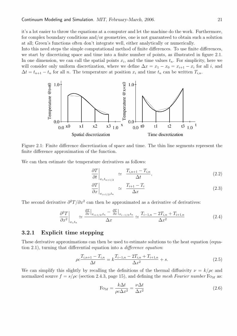
it’s a lot easier to throw the equations at a computer and let the machine do the work. Furthermore,for complex boundary conditions and/or geometries, one is not guaranteed to obtain such a solutionat all; Green’s functions often don’t integrate well, either analytically or numerically.Into this need steps the simple computational method of finite differences. To use finite differences,we start by discretizing space and time into a finite number of points, as illustrated in figure 2.1.In one dimension, we can call the spatial points xi, and the time values tn. For simplicity, here wewill consider only uniform discretization, where we define Δx = x1 − x0 = xi+1 − xi for all i, andΔt = tn+1 − tn for all n. The temperature at position xi and time tn can be written Ti,n.
Figure 2.1: Finite difference discretization of space and time. The thin line segments represent the finite difference approximation of the function.
We can then estimate the temperature derivatives as follows:
∂T ∂t
∂T ∂x
Ti,n+1 − Ti,n ,�
Δt (2.2)
Ti+1 − Ti (2.3) � Δx
xi ,tn+1/2
xi+1/2,tn
The second derivative ∂2T /∂x2 can then be approximated as a derivative of derivatives:
∂2T ∂x2
∂T ∂T − Ti−1,n − 2Ti,n + Ti+1,n∂x ∂x xi+1/2 ,tn xi−1/2,tn (2.4) 2Δx Δxxi ,tn
3.2.1 Explicit time stepping
These derivative approximations can then be used to estimate solutions to the heat equation (equation 2.1), turning that differential equation into a difference equation:
Ti,n+1 − Ti,n Ti−1,n − 2Ti,n + Ti+1,n + s. (2.5) ρc = k
Δt Δx2
We can simplify this slightly by recalling the definitions of the thermal diffusivity ν = k/ρc and normalized source f = s/ρc (section 2.4.3, page 15), and defining the mesh Fourier number FoM as:
kΔt νΔt FoM = = (2.6)
ρcΔx2 Δx2

� �
22 Continuum Modeling and Simulation. MIT, FebruaryMarch, 2006.
(recall ν is the thermal diffusivity k/ρc), so a rearranged equation 2.5 becomes:
Ti,n+1 = Ti,n + Δt νTi−1,n − 2Ti,n + Ti+1,n
+ s
= Ti,n + FoM (Ti−1,n − 2Ti,n + Ti+1,n) + f Δt (2.7) Δx2 ρc
This gives us a nice algorithm for computing the temperatures at the next timestep from those of the previous timestep and those on the boundaries. This algorithm is called explicit timestepping, or the Forward Euler timestepping algorithm. It is so straightforward that we can even do it in a simple spreadsheet. But its key drawback is that for large time step sizes, it is unstable, as discussed below.
Explicit timestepping stability criterion
We can regroup the terms on the right side of equation 2.7 to express the temperature in the new timestep as follows:
Ti,n+1 = Ti,n(1 − 2FoM ) + 2FoM Ti−1,n + Ti+1,n
+ f Δt. (2.8) 2
Neglecting the last term for generation, this is effectively a weighted average between Ti,n and the mean of its two neighbors: if FoM = 0, then Ti,n+1 = Ti,n (goes nowhere); if FoM = 1 , then
2 1Ti,n+1 = 2 (Ti−1,n + Ti+1,n) (mean of the neighbors); if FoM is between 0 and 1 then Ti,n+1 will
2 1be between these two. But if FoM > 2 , then the new temperature goes beyond the mean of the
neighbors. This makes the solution unstable, as oscillations in the solution will grow geometrically with each timestep, as shown in figure 2.2.
Figure 2.2: “Overshoot” of the average neighboring temperature for FoM > 0.5; growth of an oscillation for FoM = 0.7 with T0 and T4 fixed as boundary conditions (the dark curve is the initial condition).
This result gives the explicit timestepping stability criterion as FoM ≤ 1 , and restricts the choice 2
of Δx and Δt. Written in terms of Δt, this criterion is:
Δx2
Δt ≤ . (2.9) 2ν
Note that in two dimensions with a square grid, there are four neighbors, and the criterion becomes 1FoM ≤ 4 ; in three dimensions, FoM ≤ 1 . Equation 2.9 implies that if one makes the spatial
6 discretization twice as fine (cutting Δx in half), then the timestep must be reduced by a factor of four, requiring eight times the computational work to simulate the same amount of total time.

� �
Continuum Modeling and Simulation. MIT, FebruaryMarch, 2006. 23
3.2.2 Implicit Timestepping
Explicit timestepping is a simple algorithm for doing timestepping. Unfortunately, the explicit stability criterion places a very strict limit on the timestep size, making computation very expensive for any decent mesh spacing, but there are methods which can use much much bigger timesteps. First, explicit timestepping extrapolates the spatial derivatives at the present time forward, resulting in an instability. So why not calculate the future value and use that to interpolate backward? This is the implicit timestepping algorithm, also known as backward Euler time integration, and it does not have the instability associated with the explicit algorithm. To revisit the example of finite difference simulation of heat conduction, the explicit discretization looks like:
Ti,n+1 − Ti,n Ti−1,n − 2Ti,n + Ti+1,n + fi, (2.10) = ν
Δx2Δt where fi is the normalized source term si/ρc at grid point i. With implicit finite differencing, the time indices on the right side change:
Ti,n+1 − Ti,n Ti−1,n+1 − 2Ti,n+1 + Ti+1,n+1 + fi. (2.11) = ν
Δx2Δt
Of course, the new temperatures in timestep n + 1 are unknown, so how do we calculate these derivatives? The answer is that we don’t, explicitly, but we use these as a set of simultaneous equations which we can solve using linear algebra. For the equation above, we can multiply by Δt and rearrange to give:
νΔt νΔt νΔt Ti−1,n+1 + 1 + 2 Ti,n+1 − Ti+1,n+1 = fiΔt + Ti,n. (2.12) −
Δx2 Δx2 Δx2
This is the equation for one specific interior node; using the mesh Fourier number definition FoM = νΔt/Δx2, and setting temperature boundary conditions at x0 and x4 to T0,BC and T4,BC respectively, we can write this equation for an aggregate of nodes: ⎞⎛⎞⎛⎞⎛
1 0 0 0 0 T0,n+1 T0,BC ⎜⎜⎜⎜⎝
⎜⎜⎜⎜⎝
⎟⎟⎟⎟⎠
T1,n+1
T2,n+1
T3,n+1
⎟⎟⎟⎟⎠=
⎜⎜⎜⎜⎝
f1Δt + T1,n
f2Δt + T2,n
f3Δt + T3,n
⎟⎟⎟⎟⎠. (2.13)
−FoM 1 + 2FoM −FoM 0 0 0 1 + 2FoM−FoM
0 −FoM 0
1 + 2FoM0 −FoM
0 −FoM
10 0 0 T4,n+1 T4,BC
This reduces our difference equations to a simple linear system which we can solve using linear algebra techniques, such as multiplying both sides by the inverse of the matrix on the left. Implicit timestepping is unconditionally stable. If we take the limit as Δt goes to infinity, we can divide equations 2.12 and 2.13 by the mesh Fourier number, so the 1s in the matrix diagonal and the Ti,n on the right side vanish, and we obtain the steadystate result. The downside is that it is considerably more complex to implement than explicit timestepping. Furthermore, this approach leads to errors on the order of the timestep size. But it is not hard to obtain quadratic or higher accuracy using both explicit and implicit time stepping algorithms known as AdamsBashforth and AdamsMoulton methods, of which the next section presents one example.
� �
�
�
Continuum Modeling and Simulation. MIT, FebruaryMarch, 2006. 24
3.2.3 SemiImplicit Time Integration
Common to explicit and implicit timestepping is the assumption of constant time derivative throughout the timestep. If we acknowledge that the value of ∂T/∂t may be changing within the timestep,we can achieve better accuracy.The simplest such approach, known as semiimplicit or CrankNicholson timestepping, involveslinear interpolation of ∂T/∂t between timesteps n and n + 1. Another way to look at this is that itestimates the value of ∂T/∂t at timestep n + 1 . Either way, for the heat equation, we average the
2 right hand sides of equations 2.10 and 2.11 to give:
Ti,n+1 − Ti,n ν Ti−1,n − 2Ti,n + Ti+1,n + Ti−1,n+1 − 2Ti,n+1 + Ti+1,n+1 fi,n + fi,n+1 . (2.14) = +
Δt 2 Δx2 2 By treating the derivative as linear over the timestep, the error becomes secondorder in the timestep size (that is, proportional to Δt2). This is considerably more accurate than explicit or implicit timestepping, while more stable than explicit timestepping. However, because this average includes the previous timestep, this method is not unconditionally stable (as implicit timestepping is).
3.2.4 AdamsBashforth
If first order accuracy of explicit and implicit methods are good (like straight Riemann integration),and second order semiimplicit is better (like trapezoid rule integration), why not go on to Simpson’srule for third or higher order discretizations? There are three approaches to accomplishing highorder accuracy in timestepping: an explicit method called AdamsBashforth, an implicit methodcalled AdamsMoulton, and a very efficient method with multiple function evaluations per timestepcalled RungeKutta.This explicit higherorder method uses previous timesteps to extrapolate the ∂T/∂t curve into thenext timestep. The simplest such method is just explicit timestepping, which is firstorder in time,and can be expressed as:
un+1 = un + Δtf(un), (2.15) where u is the unknown variable or set of variables (such as the values of temperature Ti), and
∂u = f(u). (2.16)
∂t This is analogous to equation 2.7. For higherorder accuracy, one can use previous timesteps, e.g. we can use this and the previous timestep to extrapolate a linear function of ∂T/∂t to achieve quadratic accuracy like semiimplicit timestepping; with uniform Δt, this is written generally as:
3 1 un+1 = un + Δt f(un)− f(un−1) . (2.17)
2 2
In general, for polynomial order p: p−1
un+1 = un + Δt ap,j f(un−j ), (2.18) j=0
where ap,j = 1 for any p. This has the advantages of being explicit and solvable without simultaneous equations, while also very accurate, and the function f(u) need only be evaluated once per timestep. The disadvantage is that like explicit/forward Euler time stepping, this method is only stable for suitably small timesteps.
� �
�
� �
� �
Continuum Modeling and Simulation. MIT, FebruaryMarch, 2006. 25
3.2.5 AdamsMoulton
This implicit cousin of AdamsBashforth time integration interpolates from previous timesteps and the next to provide a polynomial fit estimating ∂T/∂t. Again, the firstorder accurate version is the same as implicit/backward Euler time stepping, and the secondorder accurate version is identical to semiimplicit/CrankNicholson. For a thirdorder accurate version, we interpolate two old timesteps and the new one to give a quadratic polynomial estimate of ∂T/∂t, which integrates to give thirdorder accuracy. With uniform Δt, this is written:
5 8 1 un+1 = un + Δt f(un+1) + f(un)− f(un−1) . (2.19)
12 12 12
In general for polynomial order p:
p−1
un+1 = un + Δt ap,j f(un−j+1) (2.20) j=0
This is more accurate and more stable than AdamsBashforth, but as with the comparison between implicit and explicit timestepping, is harder to implement. There is one (non)linear solution per timestep, with as many function evaluations as necessary to solve the system.
3.2.6 RungeKutta Integration
RungeKutta integration achieves highorder accuracy by evaluating the function at multiple points within each timestep. Each function evaluation requires no simultaneous equation solution, giving it this advantage over implicit and AdamsMoulton methods. Though a general method, the most often used version is fourthorder accurate, which looks like::
Δt un+1 = un + (k1 + 2k2 + 2k3 + k4), (2.21)
6
where:
k1 = f(un), (2.22) Δt
k2 = f un + k1 , (2.23) 2
Δt k3 = f un + k2 , (2.24)
2 k4 = f(un + Δtk3). (2.25)
This takes more time than explicit or AdamsBashforth methods, particularly if function evaluations are expensive (which they are not for the heat equation), but doesn’t require solution of any simultaneous equations.
3.3 Enthalpy Method
When a phase boundary is present in a system, it is necessary to change the formulation somewhat to account for it. Fortunately, for liquidsolid systems there is a relatively simple method for doing

� � � �
26 Continuum Modeling and Simulation. MIT, FebruaryMarch, 2006.
this called the enthalpy method, which is based on tracking the enthalpy change at the liquidsolid interface. The enthalpy uses the relation ΔH = ρcpΔT , where cp is the constantpressure heat capacity. The 1D enthalpy conservation equation goes:
∂H ∂2T = k . (3.26)
∂t ∂x2
This is very similar to equation 2.1.In the enthalpy method, we turn that differential equation directly into a difference equation; withexplicit timestepping, this looks like:
Hi,n+1 − Hi,n =
k ∂T ∂x i+ 1
2 k ∂T
,n −
∂x i− 1 2,n
+ s (3.27) Δt Δx
ki+ ,n(Ti+1,n − Ti,n)− ki− 1 2,n(Ti,n − Ti−1,n)
+ s. 1 2 =
Δx2
and ki−phases with potentially quite different conductivities.
22Keeping the ki+ distinct is necessary because the two sides may be in the different 1 1 ,n ,n
A basic implementation of this stores two fields: H and T . In each timestep, the new H values are calculated from the old H and the old neighboring T values. The new T values are then calculated from the new H values using the inverse of the H(T ) function.1
This “basic implementation” in one dimension is straightforward to insert into a spreadsheet, as provided for use with Problem Set 2 part 1. It is interesting to watch this simulation in action: during freezing, the moving liquidsolid interface appears to be “pinned” at a spatial location as the enthalpy decreases with no corresponding change in the temperature. This explicit timestepping formulation (in equation 3.27) will have a stability criterion for the same reason as the nonenthalpy method, and in fact, if the two phases have the same properties, the stability criterion will be the same as equation 2.9. If the two phases have different properties, then the one with the larger ν will have the smaller critical Δt, and choosing that smaller Δt will satisfy the stability criterion in both phases. (Note that at the interface itself, the heat capacity is essentially infinite, so ν = 0 and it is stable for any timestep size.)
3.4 Finite Volume Approach to Boundary Conditions
The finite volume approach is slightly different from finite differences, and I like it because of its elegant approach to presenting boundary conditions. Rather than thinking of the spatial discretization as a set of points, the finite volume approach considers a set of regions, or elements, and considers the average temperature or enthalpy in each element. The heat conservation equation in the enthalpy method can then be written as:
∂H � V = − Aiqi + V s, (4.28) ∂T
1One may also avoid storing the T values by calculating those of the previous timestep from H on the fly (though this makes postprocessing the resulting data less straightforward). Although one can store only H and calculate T from that, in many cases one may not store only T and calculate H because H is not a unique function of T , e.g. in a pure material at the melting temperature, H can not be determined.

27 Continuum Modeling and Simulation. MIT, FebruaryMarch, 2006.
where V is the volume of the element (length in one dimension), the Ai are the areas of its faces (one in one dimension), and the qi are the outward normal fluxes through those faces. At an interior point or volume, this and the finite difference method both give the same results, expressed in equations 2.5 and 3.27. Based on this, one can very easily express a heat flux boundary condition, or a mixed condition where flux is a function of temperature. A common boundary condition of that type involves a heat transfer coefficient labeled as h:
q · ˆ� n = h(T − Tenv ), (4.29)
where Tenv is an environment temperature. This is often known as a convective boundary condition, based on boundary layer theory of transport in a fluid adjacent to a solid. These types of boundary conditions are straightforward to implement in finite volumes. Note however that this leads to a new stability criterion at the interface, which will put a limit on Δt similar to that in equation 2.9; derivation of this expression is left as an exercise to the reader. What is not straightforward with this approach is setting a surface temperature. To do this requires setting the flux such that the temperature at the outside face is equal to the desired temperature. One can think of this in terms of a “virtual volume” outside the domain where the temperature is reflected through the desired surface temperature. Referring again to the spreadsheet, its two boundary conditions are zero flux and convective, making this finite volume approach the logical one. You can see the finite volume implementation in the enthalpy elements on the left, and its boundary conditions on each side, but note that the widths of the boundary elements are half of those of the interior elements. The castabox software, also on the website, also uses flux boundary conditions, based on both convective and radiative fluxes (both on the top surface, convective everywhere else). (castabox also has an interesting calculation for the stability criterion in three dimensions.) Finally, note that the finite volume approach can be considered a “zeroorder finite element” approach, whose firstorder cousin will be introduced in the next chapter, with higherorder variants coming later.

�
�
�
Chapter 4
Weighted Residual Approach to Finite Elements
The weighted residual approach can be used to compute the approximate solution to any partial differential equation, or system of equations, regardless of whether it can be expressed as the minimum of a functional. This approach, also called the Galerkin approach, will be used later to discuss modeling of mechanics and fluid flow, and also forms the basis of the Boundary Element Method (BEM) – and in a sense, the Quantum section of the course.
4.1 Finite Element Discretization
In the finite difference section, we discussed the finite volume approach, in which we consider each cell to have a single average value of temperature (and/or enthalpy). The approximation of the field variable is thus a set of zeroorder steps, and the difference between this approximation and the real temperature has errors on the order of the mesh spacing. In finite elements, shapefunctions are piecewiselinear, resulting in higher accuracy; just as the trapezoid rule for integration has errors on the order of the grid spacing squared. In both finite volume and linear finite element approaches, we consider the approximation of a field variable, such as temperature, using the sum:
N
T � T̃ = TiNi(�x), (1.1) i=1
where Ni(�x) is a shapefunction which has the property:
1, �x = �xiNi(�x) = x = �xj=i
, (1.2) 0, �
where �xi and �xj are the node points, or gridpoints, in the simulation mesh. In one dimension,zeroorder elements (finite volume) have a single “gridpoint” on each element, and linear elementshave gridpoints on each end.In two or more dimensions, it is helpful to transform each element to local coordinates, typicallywritten as ξ� with coordinates ξ, η (and in three dimensions ζ). For example, linear triangle elements
28

�
� �
�
� �
Continuum Modeling and Simulation. MIT, FebruaryMarch, 2006. 29
often use a local coordinate system based on the unit right triangle. Then in the local coordinates with gridpoints 1, 2, and 3 at the origin, (1,0) and (0,1) respectively, we have:
N1 = 1− ξ − η, N2 = ξ, (1.3) N3 = η.
We can transform these coordinates back into the reference frame using something like equation 1.1:
3
�x = �xiNi(ξ�), (1.4) i=1
for example, if ξ� = (1, 0), then N1(ξ�) = 0, N2(ξ�) = 1, N3(ξ�) = 0, so �x = �x2. Likewise:
1 1 ξ� = , ⇒ N1(ξ�) = N2(ξ�) = N3(ξ�) =
1 , (1.5)
3 3 3
and �x is just the average of the three corners, which is the centroid of the element.It is then natural to extend this to secondorder elements by considering elements with three gridpoints in each direction: one on each end and one in the middle. In quadratic (and higherorder)square elements we typically use local element coordinates ξ ∈ [−1, 1], η ∈ [−1, 1], so the shape
1functions are products of ξ(ξ − 1), 1 − ξ2 and 1 ξ(ξ + 1). For example, the fourth shapefunc2 2
tion in a quadratic square element (3 nodes × 3 nodes), corresponding to the fourth node where ξ = −1, η = 0, is
N4(ξ�) =1 ξ(ξ + 1)(1− η2).
2
4.1.1 Galerkin Approach to Finite Elements
Thus far, we can estimate the field variable and provide a coordinate transformation from elemental to real coordinates. To set up the finite element calculation itself, we can either use the variational formulation discussed by Franz Ulm which minimizes a quantity such as overall energy, or if we have the equation to solve, then the Galerkin weightedresidual approach can be simpler in some ways. For steadystate heat conduction where the partial differential equation is �2T = 0, this approach defines a residual function as:
Ri(T1, T2, ..., TN ) = φi(�x)�2 T̃ dA, (1.6)
where φi is a weighting function. If we solve the simultaneous equations to set all of the Ri functions to zero, then we will have a set of temperatures T1, ..., TN which comprise an approximate solution to the equation �2T = 0. Right away we see there is a problem, because at the element boundaries, the shapefunction derivative �φi is not continuous, so its second derivative �2φi is not integrable; the same goes for the second derivative of T̃ since that is expressed in terms of the shapefunctions. We can solve this problem using integration by parts:
Ri = T )dA − T dA. (1.7) � · (φi� ˜ �φi · � ˜

�� � � ��� � � �
� �
30 Continuum Modeling and Simulation. MIT, FebruaryMarch, 2006.
This integral is one we can do with the existing shapefunctions. In typical finite element simulations, we use those shapefunctions Ni for the weighting functions φi, but that will not be true of boundary elements, which will be discussed presently. To do the overall integral, we can just add the integrals on each element. But to do the element integrals in local element coordinates, we must be able to write dA in terms of dξ and dη, which we can do using the cross product of the coordinate gradients from equation 1.4:
dA =∂x ∂y ∂ξ ∂ξ ∂x ∂y ∂η ∂η
dξdη. (1.8)
This matrix is called the Jacobian, and its determinant represents the scaling between the differential areas in the two coordinate systems. In three dimensions, the determinant of the Jacobian corresponds to the triple product of the gradients, and likewise scales the differential volumes. The integration in equation 1.6 is typically performed using Gaussian integration, in which the integral is expressed as a weighted sum of function values at different points:
f (x)dx = wif (xi), (1.9)
where wi are the integration weights and xi the integration points. Integrating over an interval with N points allows us to perfectly integrate a 2N + 1order polynomial, but the math for doing this is beyond the scope of this lecture. I refer you to Numerical Recipies for further details. This all works well for quadratic elements, but for higherorder elements, we need to put the nodes not evenlyspaced, but bunched closer toward the ends. The optimal distribution is at the GaussLobatto integration points. So we can now do great finiteelement calculations with arbitrarily high accuracy, as many as ten decimal places if we please. Unfortunately, the constitutive equations and parameters (e.g. thermal conductivity) are typically only known to a couple of decimal places, if that. So for the rare calculation where the equation must be solved exactly, highorder polynomial elements, sometimes referred to as “spectral elements”, are useful; for most thermal, mechanics and fluids calculations, we just use linear or quadratic elements.
4.2 Green’s Functions and Boundary Elements
Green’s functions are tools used to solve (partial) differential equations of the form:
Lu + f = 0, (2.10)
where L is a linear operator, f is a “source” function, and u is the unknown field variable. For example, back to the (steadystate) heat equation, L becomes k�2 (or � · (k�) for nonuniform k) and f becomes q̇, bringing back the familiar equation:
� · (k�T ) + q̇ = 0. (2.11)
The Green’s function u∗ is the solution to the equation:
Lu ∗+δ(�x − �x�) = 0, (2.12)
� �
Continuum Modeling and Simulation. MIT, FebruaryMarch, 2006. 31
where �x� is a reference point, and the delta function is defined such that:
x� ∈ Ω,δ(�x − �x�)d�x =
1, � (2.13) 0 otherwise.Ω
The Green’s function can be used by itself, or in the boundary element method. Both of those uses will be explored further in lecture.
4.3 Fourier Series Methods
This roughly corresponds to the “modal analysis” as described by Franz Ulm, as opposed to “direct time integration”, in that the matrix describing the system is diagonalized due to the weakinteractions between the various waves.This is most straightforwardly illustrated in Fourier series solution of the heat equation.Unfortunately, due to insufficient time this topic was not covered this year. A future version ofthese notes may include a complete section on fourier methods.
Chapter 5
Linear Elasticity
This lecture note continues our investigation of continuum modeling and simulation into linear ealstic problems. We start with an interesting analogy that can be made between the 1D heat diffusion problem and 1D elasticity. We then have a closer look on the physics of the problem, and develop the basis of the Finite Element Method for elasticity problems: the principle of virtual work. By way of application we investigate the water filling of a dam by means of finite element simulations.
5.1 From Heat Diffusion to Elasticity Problems
How to start?
5.1.1 1D Heat Diffusion – 1D Elasticity Analogy
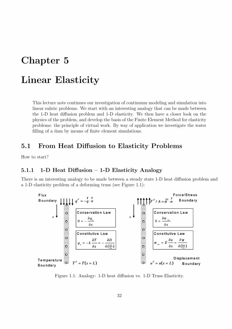
There is an interesting analogy to be made between a steady state 1D heat diffusion problem and a 1D elasticity problem of a deforming truss (see Figure 1.1):
Figure 1.1: Analogy: 1D heat diffusion vs. 1D Truss Elasticity.
32

� �
33 Continuum Modeling and Simulation. MIT, FebruaryMarch, 2006.
1. Boundary Conditions: The boundary conditions in the heat problem are either temperature or heat flux boundary conditions; and in the 1D truss problem they are either displacement boundary conditions or a force boundary condition;
deither : T d = T (0/L) ⇒ u = u (0/L)x = 0; x = L :
or : qd = −qx F d/S = σ (1.1) ⇒
where ud is a prescribed displacement, F d a prescribed force (positive in tension, whence the difference in sign wrt the heat problem), S is the surface, so that σ is a force per unit surface, that is stress.
2. Conservation Law: The conservation law in the heat problem is the energy conservation, and in the 1D truss problem it is the conservation of the momentum:
∂qx ∂σ 0 < x < L : 0 = − 0 = (1.2)
∂x ⇒
∂x
3. Constitutive Law: The constitutive law in the heat problem is Fourier’s Law, linking the heat flux to the temperature gradient; and the constitutive law in the 1D truss problem is a link between the stress and the displacement gradient, which is known as Hooke’s Law:
∂T ∂u qx = −k σ = E (1.3)
∂x ⇒
∂x
E is the Young’s modulus. The displacement gradient is called strain ε = ∂u . Alternatively, ∂x
the constitutive analogy can be made using potential functions:
∂ψ ∂ψ ∂Dqx = −
∂ �
∂T � ⇒ σ =
∂ �
∂u � = (1.4)
∂ε ∂x ∂x
where ψ is the socalled free energy (or Helmholtz energy). For instance for a linear elastic material, ψ reads: � �2
1 ∂u 1 ψ = E = Eε2 (1.5)
2 ∂x 2
It is readily understood that ψ is a convex function of its argument (the displacement gradient), so that:
∂ψ (ε∗ − ε) ≤ ψ (ε∗) − ψ (ε) (1.6)
∂ε For a linear elastic material, strict convexity has an obvious physical meaning: the stiffness E must be greater than zero,
∂2ψ E = > 0 (1.7)
∂ε2

� �
� � � �
� �
Continuum Modeling and Simulation. MIT, FebruaryMarch, 2006. 34
5.1.2 3D Extension
The heat diffusion – elasticity analogy holds also for the 3D situation, if we make the link in between the 3D counterparts of the 1D quantities. This analogy is given by:
T u = u−→→−→q σ= q →
−−−→� T = lim gradT ε = u� s−→ = 1
2 Tlim gradu + (lim gradu)
(1.8)→
∂ψ Fourier�s law : q =
∂D Hooke�s law : σ =−
∂ (lim gradT ) →
∂ε Heat balance : lim divq = 0 Momentum balance : lim divσ = 0→
There are some important differences to be noted when we go from 1D to 3D:
Figure 1.2: Deformation Modes: Stretching (left), Distortion (right).
1. The elasticity analogous of the temperature T , which is a scalar, is the displacement vector, which in 3D has three components. As a consequence, the quantities that intervene in the elasticity problem are all of a higher spatially order. For instance, the analogous of the temperature gradient, which is a vector, is the symmetric part of the displacement gradient
u . Since the displacement is a vector (or 1st order tensor), the gradient of this vector is� s−→a 3 × 3 strain matrix (or 2nd order tensor): ⎤⎡
∂ux 1 ∂ux ∂uy 1 ∂ux ∂uzεxx = εxy = + εxz = +
ε =
⎢⎢⎢⎢⎢⎢⎣
⎥⎥⎥⎥⎥⎥⎦
(1.9)
∂x 2 ∂y ∂x 2 ∂z ∂x ∂uy 1 ∂uy ∂uz
ε∗ yy = ε +yz =
∂y 2 ∂z ∂y ∂uz
ε∗ = zzsym ∂y
The diagonal terms of this matrix represent relative length variations, and the outofdiagonal terms are shear strains representing distortions. Their geometrical significance is sketched in figure 1.2.
� � �� �
35 Continuum Modeling and Simulation. MIT, FebruaryMarch, 2006.
2. The analogous of the heat flux vector −→q , is a symmetric 3 × 3 stress matrix (or 2nd order tensor), σ: ⎤⎡
σxx σxy σxz
σ = ⎣yz ⎦ (1.10)σ σyy
sym σzz
The stress is at equilibrium if it satisfies the momentum balance equation:
lim divσ + ρ−→g = 0 (1.11)
where ρ is the mass density and −→g is the earth acceleration vector. For instance, water at hydrostatic equilibrium has as stress: ⎤⎡
1 0 0 σ = p− ⎣ ⎦ (1.12)1 0
sym 1
where p is the fluid pressure. The momentum balance of water at rest thus reads:⎛ ⎞⎛ ⎞∂⎜⎜⎜⎜⎝
⎟⎟⎟⎟⎠
∂x∂∂y
gx
p + ρw ⎝ ⎠ = 0 (1.13) − gy
gz∂ ∂z
where (gx, gy , gz ) are the components of the acceleration vector. Solids (or moving fluids) have in addition shear stresses, and the momentum balance (1.11) reads:
∂σxx
∂x + ∂σxy
∂y + ∂σxz
∂z + ρgx = 0 (1.14)
∂σxy
∂x + ∂σyy
∂y + ∂σyz
∂z + ρgy = 0 (1.15)
∂σxz
∂x + ∂σyz
∂y + ∂σzz
∂z + ρgz = 0 (1.16)
3. The constitutive analogous of Fourier’s Law is Hooke’s Law. Similarly to Fourier’s law, which provides a link between the heat flux vector and the temperature gradient, Hooke’s law provides a link between the stress matrix and the strain matrix. This link needs to account for the possible deformation and energy modes the material can undergo. Here we restrict ourselves to the isotropic situation: Isotropy means that the behavior has no privileged direction. In this isotropic case, we need to consider the two deformation modes shown in figure 1.2, by means of two elasticity constants:
λ �2 ψ = lim trε + µ lim tr εε ·
2 (1.17)
where lim trε = εxx + εyy + εzz is the sum of the diagonal terms in (1.9), while lim tr ε isε · the sum of the diagonal terms of the matrix product ε · ε. λ and µ are called Lamé constants, and are related to the Young’s modulus by:
λ = νE
(1 + ν) (1 − 2ν) ; µ =
E 2 (1 + ν)
(1.18)
�
� �
Continuum Modeling and Simulation. MIT, FebruaryMarch, 2006. 36
where −1 ≤ ν ≤ 0.5 is the Poisson’s ratio, a dimensionless number which captures essentially the volumetric versus the shear deformability of an isotropic material. For instance, ν = 0.5 corresponds to an incompressible material, lim trε = 0, for which λ → ∞. Using the free energy expression (1.17), the stressstrain (or displacement gradient relation) is readily obtained:
∂ψ � � σ = = λ lim trε lim diag [1] + 2µε (1.19)
∂ε
Here, lim diag [1] stands for a 3 × 3 diagonal unit matrix.
Provided these (minor, but important) differences the analogy (1.8) is readily put to work.
5.2 The Theorem of Virtual Work
Hold on... what’s about the physics?
5.2.1 From the Theorem of Virtual Work in 1D to Finite Element Formulation
We start with the 1D truss problem displayed in figure 1.1. The work that is provided from the outside to the system is:
Wext = F d u + F u d = σu dS (2.20) S
dwhere F d stands for prescribed forces and u for prescribed displacements at the boundary S, i.e. on x = 0 and x = L. This work must be equal to the work done in the inside of the truss, which we obtain by application of the divergence theorem (in 1D): � x=L ∂
� x=L ∂σ ∂u Wext = Wint = (σu) dx = u + σ dx (2.21)
∂x ∂x x=0 ∂x x=0
The stress satisfies the momentum balance ∂σxx = 0, so that the equality of the external and the ∂x
internal work realized by the stress σxx reads: � x=L ∂u � x=L
F d u + F u d = σ dx = σε dx (2.22) x=0 ∂x x=0
Expression (2.22) is the 1D version of the theorem of virtual work. Note that the stress and the displacement gradient are not yet related by a material law of the form (1.3) or (1.4). So we can apply this theorem with any other displacement u∗ (x), which satisfies the displacement boundary condition:
d u∗ (L) = u (2.23)
This yields: � x=L
F d u∗ + F u d = σε∗ dx (2.24) x=0

�
�
� �
37 Continuum Modeling and Simulation. MIT, FebruaryMarch, 2006.
Subtracting (2.22) from (2.24) yields: � x=L
F d (u∗ − u) = σ (ε∗ − ε) dx (2.25) x=0
It is only at this stage that we introduce the constitutive relation (1.4), which links the stress solution σ with the displacement gradient solution ∂u
∂x , so that the integrand of (2.25) reads:
∂ψ σ (ε∗ − ε) = (ε∗ − ε) (2.26)
∂ε
We can now make use of the convexity property (1.6) of the free energy ψ on the right hand side of (2.26), and substitute this inequality into (2.25). We so obtain � x=L
F d (u∗ − u) ≤ [ψ (ε∗)− ψ (ε)] dx (2.27) x=0
and after rearrangement: � x=L � x=L
ψ (ε) dx − F d u ≤ ψ (ε∗) dx − F d u∗ (2.28) x=0 x=0
The difference between the overall free energy contained in the truss and the work provided by prescribed forces is the potential energy, and is denoted by Epot (u). What inequality (2.28) then shows is that among all possible displacement solutions u∗ (x) that satisfy the displacement boundary condition (2.23), the solution u (x) minimizes the potential energy: �� x=L
Epot (u) = min ψ (ε∗) dx − F d u∗ (2.29) u∗=ud lim onS x=0
By analogy with the heat diffusion problem, we discretize the continuous displacement field by: M +1
u∗ (x) = uiNi(x) (2.30) i=0
where ui are nodal displacements, and Ni(x) are the base functions. For a linear elastic material for which ψ (ε∗) is given by (1.5), the potential energy reads:
M M� x=L � �2 �� 11 ∂u∗
Epot (u∗) = E dx − F d u∗ = uiKi,j uj − Fi
d u∗ i (2.31)
2 ∂x 2x=0 i=1 j=1
where Kij are elements of the stiffness matrix: � x=L ∂Ni ∂NjKi,j = E dx (2.32)
∂x ∂x x=0
Then, in order to find the minimum of the potential energy Epot (u∗), which comes the closest to
the potential energy of the solution Epot (u), we minimize (2.31) wrt the displacement degrees of freedom ui, and obtain a system of M linear equations:
M∂Epot (u
∗) = 0
� Kij uj − Fi
d = 0 (2.33) ∂ui
⇒ j=1
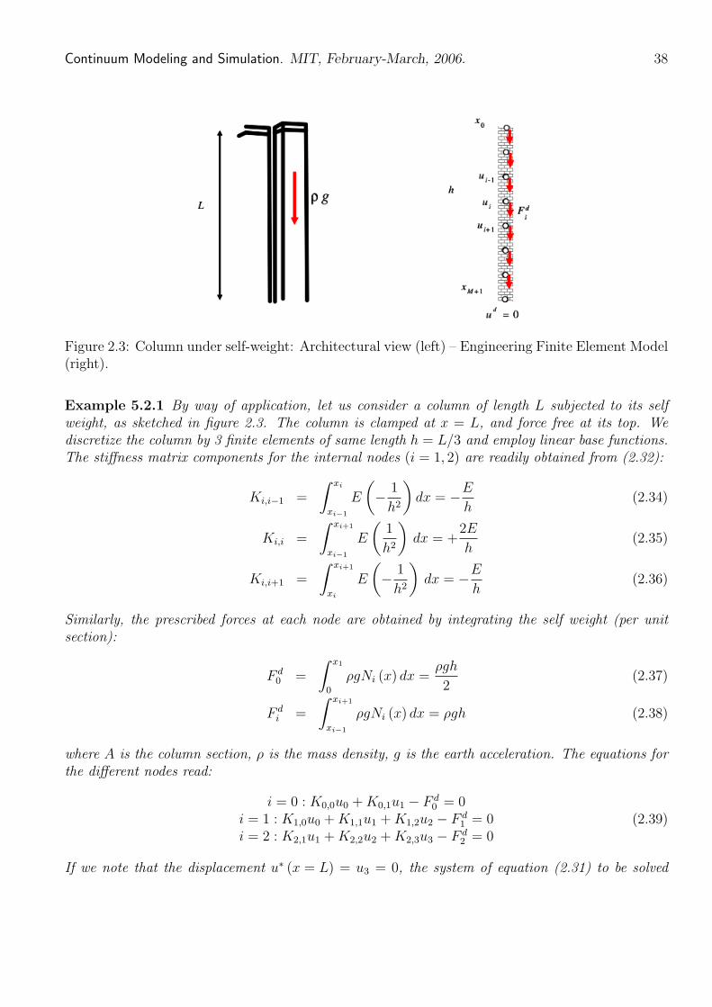
� � �
�
38 Continuum Modeling and Simulation. MIT, FebruaryMarch, 2006.
Figure 2.3: Column under selfweight: Architectural view (left) – Engineering Finite Element Model (right).
Example 5.2.1 By way of application, let us consider a column of length L subjected to its self weight, as sketched in figure 2.3. The column is clamped at x = L, and force free at its top. We discretize the column by 3 finite elements of same length h = L/3 and employ linear base functions. The stiffness matrix components for the internal nodes (i = 1, 2) are readily obtained from (2.32):
xi 1 E Ki,i−1 = E dx =−
h2 − h
(2.34) �xi−1 � � xi+1 1 2E Ki,i = E
h2 dx = + (2.35)
h � xi−1 � � xi+1 1 E
Ki,i+1 = E − h2
dx = − h
(2.36) xi
Similarly, the prescribed forces at each node are obtained by integrating the self weight (per unit section):
F d = x1
ρgNi (x) dx = ρgh
(2.37) 0 2�0 xi+1
F d = ρgNi (x) dx = ρgh (2.38) i xi−1
where A is the column section, ρ is the mass density, g is the earth acceleration. The equations for the different nodes read:
i = 0 : K0,0u0 +K0,1u1 − F d = 0 0
i = 1 : K1,0u0 +K1,1u1 +K1,2u2 − F d = 0 (2.39) 1
i = 2 : K2,1u1 +K2,2u2 +K2,3u3 − F d = 0 2
If we note that the displacement u∗ (x = L) = u3 = 0, the system of equation (2.31) to be solved

�
�
�
�
�
�
�
�
�
��
�
39 Continuum Modeling and Simulation. MIT, FebruaryMarch, 2006.
reads: ⎞⎛⎞⎛⎞⎛⎤⎡ 1 −1 0
2u0 1 0
E ρgh ⎣ ⎝⎦ ⎠ ⎝ 2⎠ =⎝ 0⎠ (2.40)−10
−12
−u1h 2
2 0u2−1
Using standard tools of solving linear system of equations, we obtain: ⎞⎛⎞⎛⎞⎛ u0 9 9
ρgh2 ρgL2 ⎝ ⎠ = ⎝ 8⎠ = ⎝ 8⎠ (2.41) u1 2E 18E
5 5u2
It is instructive to see how the solution improves as we double the number of nodes, so that h� = h/2 = L/6,with the boundary condition u∗ (x = L) = u6 = 0. The system to be solved then reads: ⎞⎛⎞⎛⎤⎡
1 −1 0 0 0 0 u�0
2 1⎢⎢⎢⎢⎢⎢⎣
⎜⎜⎜⎜⎜⎜⎝
⎥⎥⎥⎥⎥⎥⎦
⎟⎟⎟⎟⎟⎟⎠
−ρgh�
2
⎜⎜⎜⎜⎜⎜⎝
⎟⎟⎟⎟⎟⎟⎠
1−10
0 0 0−1 2
2222
u
2Eh�
−10
0 0−1 2
u= 0 (2.42)
30 −10
0−1 2
u
40 0 −10
−12
u
50 0 0 −1 2u
The solution reads: ⎞⎛⎞⎛⎞⎛ u� 36 360 ⎜⎜⎜⎜⎜⎜⎝
⎟⎟⎟⎟⎟⎟⎠
=
⎜⎜⎜⎜⎜⎜⎝
35322720
⎟⎟⎟⎟⎟⎟⎠
=ρgL2
72E
⎜⎜⎜⎜⎜⎜⎝
35322720
⎟⎟⎟⎟⎟⎟⎠
1u2ρg (h�)2u (2.43)
3 2Eu
4uu� 11 115
The solution so obtained is found not to improve the solution. Finally, a comparison with the exact solution is due. The continuous equation to be solved reads:
∂σ ∂x
+ ρg = 0 (2.44)
or equivalently using the constitutive law (1.2):
E d2u dx2
+ ρg = 0 (2.45)
Integration yields the stress solution:
σ (x) = E uρg
0 − x E
and the displacement solution: ρg 2 u (x) = u0 + u� x (2.46) 0x − 2E
where u0 and u� are two integration constants that need to be solved by boundary conditions. The 0
first boundary condition is that the stress is zero at x = 0, the second that the displacement is zero at x = L. It follows:
σ (x = 0) = 0 u� = 0 (2.47) 0⇒ ρgL2
u (x = L) = 0 ⇒ u0 = (2.48) 2E

� � � � �
� � �
� �
Continuum Modeling and Simulation. MIT, FebruaryMarch, 2006. 40
Hence, from a comparison of the FEsolutions and the exact solutions, we conclude that both discretized solutions at their respective nodal points are exact solutions. In fact, two finite element with three nodal points would have been sufficient to capture the parabolic displacement solution. Application: The World Trade Center Towers were roughly L = 400m high and A = 60 ×60m2 wide and had a weight of approximately M = 300, 000, 000kg. The average mass density can be estimated from
M kg LA
≈ 200 ρ ∼ 3m
The effective stiffness can be estimated by averaging the stiffness of the columns over the floor:
AcE = Es
A
where Es = 210GPa. The towers were built as steel tubular structural system with 4×59 box columns at the perimeter and 44 box columns in the core, thus a total of 280 columns. If we estimate that each columns has roughly a section of 0.20m2, an order of magnitude of the columntofloor section is Ac/A ∼ 2%, whence an effective stiffness in the vertical direction of E ∼ 4GPa = 4, 000, 000, 000Pa. The vertical deformation at the top of the towers should have been on the order of:
200 × 10 × 4002
u0 = = 0.04m 2 × 4, 000, 000, 000
This is really not much (u0/L = 1/10, 000), so there is not much to be worried when it comes to the vertical deformation under selfweight. The critical design loads for skyscrapers are horizontal loads: winds, earthquakes, etc.
5.2.2 Theorem of Minimum Potential Energy in 3D Linear Isotropic Elasticity
What we have seen in 1D extends to 3D linear isotropic elasticity problems, if we replace the 1D scalar quantities by their 3D counterparts. The 3D external work rate comprises two terms, the work done by volume forces (such as the gravity force vector ρ−g , as just seen in the example), and →
the work by surface traction vectors −t n :→
= σ · −→
u g dV + u n dS (2.49) Wext = → ρ− −− · → → σ · −· →V S
Application of the principle of the divergence theorem to the second term yields the internal work:1
Wint = σ : ε dV (2.50) V
1The derivation is not trivial. First of all, application of the divergence theorem reads here: � � � � � � � �− · → − · → u : σ dVu n dS = lim div u σ dV = u lim div σ + lim grad−→ σ · − → − · →S S S
If we note that σ is symmetric, we have:
lim grad− : σ = ε : σ = σ : εu→
In matrix notation, the double product ε : σ corresponds to taking the trace of the matrix product ε · σ.
ε : σ = lim tr σε ·
� � � � �
� � � � �
� � �
� �
� � � � ��
� � � � �
41 Continuum Modeling and Simulation. MIT, FebruaryMarch, 2006.
The theorem of virtual work then reads:
Wext = Wint
u g dV + u n dS = σ : ε dV (2.51) → ρ− −− · → → σ · −· →V S V
Following the 1D approach, we apply the theorem of virtual work with a second displacement field u ∗ which satisfies the displacement boundary condition: −→
− g dV + u ∗ n dS = σ : ε∗ dV (2.52) u ∗ ρ− −→ · → → σ · −· →V S V
Taking the difference of (2.51) and (2.52) yields the 3D generalization of (2.25):
→ → → → → →d dS = σ : ε∗ − ε dV (2.53) u ∗ −− g dV + (− u ) · −t � �
(− u ) · ρ− u ∗ −−V S V
where −t d is the prescribed surface traction vector. Finally, all what we are left to do is to recognize →
that the stress σ in (2.53) derives from the free energy ψ (see Eq. (1.19)), and that the free energy is a convex function of its argument ε; that is analogously to the 1D situation (1.6):
� � ∂ψ � � � � � � σ : ε∗ − ε = : ε∗ − ε ≤ ψ ε∗ − ψ ε (2.54)
∂ε
Finally, replacing the r.h.s. of equality (2.54) by the r.h.s. of inequality (2.54), we arrive, after some rearrangements, at the 3D formulation of the theorem of minimum potential energy (2.29): �� �� � ��
u ) = min ψ ε∗ dV − → g dV + u ∗ →d dS (2.55) Epot (− u ∗ ρ− → −
tu ∗ =−
→− u d lim onS
− · → − ·→ →V V S
The theorem states that among all possible displacement fields −u ∗ that satisfy the displacement →boundary conditions, the solution field − minimizes the potential energy. The first term on the u→right hand side of (2.55) represents the entire free energy which is contained in the system, and the two second terms represent the work provided from the outside through volume and surface forces.
We then obtain with (2.49):
u g dV + u lim divσ + lim tr σ dVWext = → ρ− → ε ·V V
− · → − ·
We now need to consider the local momentum balance equation, which reads in the presence of body forces (see Eq. (1.11)):
lim divσ = −ρ−g→
The first term in the external work skips out, and we find that:
Wext = lim tr σ dV = Wintε ·V
where lim tr σ represents in fact the internal work achieved by the stress σ along the displacement gradient ε.ε ·

�
Continuum Modeling and Simulation. MIT, FebruaryMarch, 2006. 42
5.2.3 3D Finite Element Implementation
Similarly to the 1D situation, we approximate the continuous displacement field through a discrete representation:
i=M +1
u ∗ = uiNi (xj ) (2.56) −→i=0
where ui represent discrete displacements at nodal points, and Ni (xj ) are the base functions. Analogously to the 1D case, we arrive at a very similar expression of the potential energy Epot (
−u ∗) as→in the 1D case:
u ∗) = uiKij uj − Fid ui (2.57) Epot (
− 1 →2
where Kij is still the stiffness matrix, and F d the external force vector which here accounts for both i
the volume forces and surface forces. As a consequence of the theorem of minimum potential energy (2.55), the problem to be solved reduces to solving a linear system of equations:
∂Epot (ui, uj )= 0 ⇒ Kij uj − Fi
d = 0 (2.58) ∂ui
We will see an interesting application here below.
5.2.4 Homework Set: Water Filling of a Gravity Dam
We consider a gravity dam of triangular shape (Height H, Top angle α) clamped on its base OA (zero displacement prescribed), see figure 2.4. The downstream surface AB is stress free. The upstream wall OB is subjected to the water pressure (body force ρw
−g ) over a height OB� = mH, where m ∈ [0, 1].→The water is at rest satisfying hydrostatic equilibrium. The remaining surface B�B is stress free. For the purpose of analysis, we assume that the gravity dam is composed of a linear isotropic elastic material (Lamé constants λ, µ) with volume mass ρd. With regard to the dimension of the gravity dam in the Oz−direction, the problem can be treated as a plane strain problem with regard to the plane parallel to Oxy. We want to evaluate the displacement of the dam along the upstream wall OB with water filling m ∈ [0, 1].
Exercise 5.2.1 First Approximation: We consider a displacement field of the form:
u ∗ = ay → −− e x + b
y →y (2.59) e→
H −
H
Using the theorem of minimum potential energy, give an approximation of the displacement along OB. Show that the problem can be recast in the format of the finite element method:
Kij uj = Fid (2.60)
where Kij are the components of the stiffness matrix, uj are the unknown nodal displacements, and F d i
are nodal forces. Determine Kij , F d and uj for the given approximation (2.59) of the displacement field i
u ∗ in the gravity dam. −→
43 Continuum Modeling and Simulation. MIT, FebruaryMarch, 2006.
Exercise 5.2.2 Finite Element Approximation: Consider m = 1, and ρd = 0. By means of the finite elements, show that the horizontal displacement solution converges with increasing number of elements. To this end, normalize the obtained displacement at y = H by
ux(x = 0, y = H) u = � � (2.61)
ρw gH2
3µ tan α
with µ the shear modulus. Represent your results in form of a graph giving u as a function of the number of elements over OB.
Image removed due to copyright reasons.
Figure 2.4: Hydroelectric Dam in Krasnoyarsk, Russia (1967). Left: Photo by Dr. A. Hugentobler; With permission from http://www.structurae.net; Right: Engineering Model.
The OneTriangle Finite Element Solution
The system we are interested is the solid dam, subjected to displacement and stress boundary conditions:
1. We need to check that the displacement field (2.59) is compatible with the boundary conditions. This is the case here:
lim onOA : − uu ∗ (x, y = 0) = − d = 0 (2.62) → →
2. We need to determine the surface tractions the upstream water exerts on the surface OB�. The stress in the water is at hydrostatic equilibrium, as defined by (1.13). In the coordinate

� � � �� � �
� � � �� �
�
44 Continuum Modeling and Simulation. MIT, FebruaryMarch, 2006.
→ →y or in vector components g esystem of the problem, the acceleration vector reads − = −g−
2(gx, gy , gz ) = (0, −g, 0), where g � 10m/s . The hydrostatic momentum balance equation then reads: ⎛ ∂ ⎞⎛
⎞
−
⎜⎜⎜⎜⎝
⎟⎟⎟⎟⎠
∂x∂∂y
0 p − ρw ⎝ ⎠ = 0 (2.63) g
0∂ ∂z
The first and the last equation show that the water pressure is a function of y only; whence after integration of the second equation:
p (y) = C − ρw g y (2.64)
where C is an integration constant, which is readily solved by considering that the water pressure on the water surface y = mH is zero:
p (y = mH) = 0 ⇒ C = ρw g mH (2.65)
The stress in the water thus reads (application of (1.12)): ⎤⎡ 1 0 0
σw = ρw g (y −mH)⎣ ⎦ (2.66)1 0 sym 1
The surface tractions the water exerts on the surface OB� is −t d = σw n = σw →e x:→ → · −· −⎞⎛⎤⎡
1 0 0 1 →d−t = σ · −n→ = ρw g (y −mH)⎣ ⎠ = ρw g (y −mH) −e x→1 0 ⎝⎦ 0 (2.67)
sym 1 0
We can now turn to the determination of the potential energy (2.55), which reads here:
·−t→u ∗)Epot (−→ − g dV + u ∗u ∗ ρd
− →→ · → − d dS (2.68) ε∗ψ dV −= V V S
x=H tan α y=H
= ψ ε∗ dxdy (2.69) x=0 y=0
x=H tan α y=H
+ ρdg (− e y ) dxdy (2.70) → · −u ∗ →
x=0 y=0 y=mH
− y=0
ρwg (y −mH) (− e x) dy (2.71) → · −u ∗ →
In some more details:The free energy in the dam needs to be evaluated from (1.17), and requires first the determinationof the strain ε∗ from (1.9). The two nonzero displacements in (2.59) read:
y u∗ = a
y ; u∗ = b (2.72) x H y H

� � � �
� �
� �
� � � � � �
� � � � � � � ��
� �
� �
�
45 Continuum Modeling and Simulation. MIT, FebruaryMarch, 2006.
The strains are obtained by substituting (2.72) in (1.9): ⎤⎡ ∂u∗ 1 ∂ux a 1 ∂ux ∂uzxε∗ = = 0 εxy = +
∂uy = εxz = + = 0 xx ∂x 2 ∂z ∂x
ε∗ =
⎢⎢⎢⎢⎢⎢⎣
= 0
⎥⎥⎥⎥⎥⎥⎦
(2.73)
2 ∂y ∂x 2H∂uy b 1 ∂uy ∂uz
ε∗ yy = ε += yz =
∂y H 2 ∂z ∂y ∂uz
ε∗ = = 0 zz sym ∂y
The strain invariants in (1.17) read:
b lim trε∗ = ε∗ + ε∗ + ε∗ = (2.74) xx yy zz H
⎞⎤⎡⎤⎡⎛ a 00 a 0 0
2H 2H ⎣⎝ ⎣⎦ ⎠⎦a b a bε∗ ε∗lim tr lim tr 0 0= · ·2H H 2H H 0 0 0 0 0 0 ⎡ ⎤
1 a2 1 a b 04 H2 2 H2
1 a 1 a2 b2⎣ ⎦lim tr b 0= +2 H2 4 H2 H2
0 0 0
1 a2 1 a2 b2 1 a2 b2
= + + = + (2.75) 4 H2 4 H2 H2 2 H2 H2
Using (2.74) and (2.75) in (1.17) yields: �2 2 b2λ �2 λ b 1 a(2.76) ψ = lim trε + µ lim tr ε = + µ +ε ·
2 2 H 2 H2 H2
The total free energy (2.69), therefore, which is contained in the dam reads: �2x=H tan α y=H 2 b2λ b 1 a(2.77) ψ ε∗ dxdy = A + µ +
2 H 2 H2 H2 x=0 y=0
1where A = H2 tan α is the section of the dam. This quantity can be rewritten in the form of the 2
finite element procedure: ⎡ ⎤µA 01 1 H2 a (2.78) ⎣ ⎦uiKij uj = (a, b) λ + 2µ b2 2 0 A
H2
The external work contributions to the potential energy (2.70) and (2.71) are developed in the form:
x=H tan α y=H
ρdg u∗ ρdg
b (2.79) y dxdy = A 3x=0 y=0
y=mH 3H2
ρw g (y − mH) u∗ ρw gma (2.80) x dy = −
6−
y=0
46 Continuum Modeling and Simulation. MIT, FebruaryMarch, 2006.
or in terms of the finite element procedure: ⎛ 3H2 ⎞ ρw gm
−Fid ui = − (a, b) ⎝ 6ρdg
⎠ (2.81) −A
3
The potential energy (2.57) is the sum of (2.78) and (2.81):
Epot (−→u ∗) =
1 2
(a, b)
⎡ ⎣ A µ H2
0
0
A λ + 2µ H2
⎤ ⎦ � a b
�
− (a, b)
⎛ ⎝ ρw gm
3H2
6 −A
ρdg 3
⎞ ⎠ (2.82)
Minimization (according to (2.58)) yields the linear system of equations:
∂Epot (a, b) ∂ (a, b)
= 0 ⇒
⎡ ⎣ A µ H2
0
0
A λ + 2µ H2
⎤ ⎦ � a b
�
=
⎛ ⎝ ρw gm
3H2
6 −A
ρdg 3
⎞ ⎠ (2.83)
The two unknowns of the problem (a, b) that minimize the potential energy are:
� a b
�
=
⎛ ⎜⎜ ⎝
ρw gm3H2
3 tan αµ ρdgH
2
⎞ ⎟⎟ ⎠ (2.84) −
3 (λ + 2µ)
The displacement a is the horizontal crest displacement and the displacement b is the vertical displacement. To evaluate an order of magnitude, let us consider a concrete dam, for which the Young’s modulus is roughly E = 30 GPa, the Poisson’s ratio ν = 0.2, so that the Lamé constants (1.18) are λ = 8.3 GPa and µ = 12.5 GPa. The water density is ρw = 1, 000 kg/m3, and the concrete density is ρd = 2, 500 kg/m3. The crest and base widths of the dam displayed in figure 2.4 is 24 m and 140 m, so that tan α = (140 − 24) /H. A lower bound estimate of the crest displacement is u∗
x (y = H) = 2. 3 × 10⁻⁹ (mH)3; for instance, for a 100 m high dam, which is fully filled (m = 1), a lower bound of the crest displacement is on the order of 3 mm (quite negligible!).
Finite Element Solution
Congratulations! We just approximated the gravity dam by one single 2D triangle element. As we refine the discretization by adding more triangle elements we come closer to the actual potential energy in the gravity dam. This is readily achieved by any commercially available finite element program. This is to be shown for m = 1 (end of water filling), and by setting the self weight of the dam to zero. The obtained crest displacement is normalized by the solution of the onetriangle element solution (2.84).
5.3 Concluding Remarks
The finite element method is nodoubt an extremely powerful engineering method, because of its flexibility to be adapted to many engineering problems. The important issues to consider are:

47 Continuum Modeling and Simulation. MIT, FebruaryMarch, 2006.
1. The starting point for the development of any FEprocedure is the physics of the continuum problem. This includes: (1) choice of a system and the boundary conditions; (2) the filed equations derived from conservation laws, and (3) the constitutive information.
2. The FEmethod explores the convexity of the constitutive law. It is on the basis of the convexity that one can translate an ‘exact’ problem into an ‘approximated’ problem. Because of the convexity the approximation should always converge to the exact solution.
Chapter 6
Discrete to Continuum Modeling
These notes give a few examples illustrating how continuum models can be derived from special limits of discrete models. Only the simplest cases are considered, illustrating some of the most basic ideas. These techniques are useful because continuum models are often much easier to deal with than discrete models with very many variables, both conceptually and computationally.
6.1 Introduction. Continuum approximations are useful in describing discrete systems with a large number of degrees of freedom. In general, a continuum approximation will not describe all possible solutions of the discrete system, but some special class that will depend on the approximations and assumptions made in deriving the continuum model. Whether or not the approximation is useful in describing a particular situation, will depend on the appropriate approximations being made. The most successful models arise in situations where most solutions of the discrete model evolve rapidly in time towards configurations where the assumptions behind the continuum model apply.
The basic step in obtaining a continuum model from a discrete system, is to identify some basic configuration (solution of the discrete model) that can be described by a few parameters. Then one assumes that the full solution of the system can be described, near every point in space and at every time, by this configuration — for some value of the parameters. The parameters are then assumed to vary in space and time, but on scales (macroscales) that are much larger than the ones associated with the basic configuration (microscales). Then one attempts to derive equations describing the evolution of these parameters in the macroscales, thus averaging out of the problem the microscales. There is a close connection between this approach, and the “quasiequilibrium” approximations that are often invoked to “close” continuum sets of equations derived using conservation laws.
For example, when deriving the equations for Gas Dynamics in Statistical Mechanics, it is assumed that the local particle interactions rapidly exchange energy and momentum between the molecules — so that the local probability distributions for velocities take a standard form (equivalent to local thermodynamic equilibrium). What exactly makes these assumptions work (in terms of properties of the governing, microscale, equations) is rather poorly understood. But that they work rather well cannot be denied. In these notes we will consider examples that are rather simpler than these ones, however, where the “local configurations” tend to be rather trivial.
48
� � 1 2
Continuum Modeling and Simulation. MIT, FebruaryMarch, 2006. 49
6.2 Wave Equations from MassSpring Systems. Longitudinal Motion.
Consider an array of bodies/particles, connected by springs, and restricted1 to move on a straight line. Let the positions of the bodies be given by xn = xn(t), with n = 0, ±1, ±2, . . ., and let Mn
be the mass of the n th particle. Furthermore, let the force law for the spring between particles n and n+ 1 be given by: force= fn+ 1
2(Δx), where Δx is the distance between the particles, and
fn+ 1 2
is positive when the spring is under tension.2
If there are no other forces involved (e.g. no friction), the governing equations for the system are:
d2
(2.1) M x = f (xn+1 − xn) − fn− 1 2(xn − xn−1) ,1n n n+dt2 2
for n = 0, ±1, ±2, . . . The simplest solution for this system of equations is equilibrium. In this case all the accelerations vanish, so that the particle positions are given by the series of algebraic equations
n− 1 2(xn − xn−1) . (2.2)0 = f (xn+1 − xn) − f1 n+
2
This is the basic configuration (solution) that we will use in obtaining a continuum approximation. Note that this is a one parameter family: if the forces are monotone functions of the displacements Δx, then once any one of them is given, the others follow from (2.2).
Before proceeding any further, it is a good idea to nondimensionalize the equations. We will assume that:
A. All the springs are roughly similar, so that we can talk of a typical spring force f , and a typical spring length L. Thus we can write � �
Δx (2.3) fn+ (Δx) = f F1 1 ,n+ L2 2
2
2 is a nondimensional mathematical function, of O(1) size, and with O(1) deriva
tives. A further assumption is that Fare nearly equal. Mathematically, this is specified by stating that:
where F 1 n+
changes slowly with n, so that two nearby springs 1 n+
n+ 1 2(η) = F (�(n+ 1/2), η) , (2.4)F
where 0 < � � 1, and F is a “nice” (mathematical) function of its two variables.
B. All the particles have roughly the same mass m, and their masses change slowly with n, so that we can write:
Mn = mM(� n) , (2.5)
where M is a nice mathematical function, with O(1) size, and with O(1) derivatives. 1By some device: say the bodies are sliding inside a hollow tube. 2If the spring obeys Hooke’s law, then f (Δx) = kn+ Δx − L , where k > 0 and L > 0 are the n+ n+ n+ n+
spring constant and equilibrium length, respectively. 1 2
1 2
1 2
1 2
� �
�
� �
Continuum Modeling and Simulation. MIT, FebruaryMarch, 2006. 50
Remark 6.2.1 Why do we need these assumptions? This has to do with the questions of validity, discussed in the introduction. Suppose that these hypothesis are violated, with the masses and springs jumping wildly in characteristics. Then the basic configuration described by (2.2) will still be a solution. However, as soon as there is any significant motion, neighboring parts of the chain will respond very differently, and the solution will move away from the local equilibrium implied by (2.2). There is no known method to, generically, deal with these sort of problems — which turn out to be very important: see remark 6.2.2.
From the assumptions in A and B above, we see that:
Changes in the massspring system occur over length scales � = L/�. (2.6)
Using this scale to nondimensionalize space, namely: and a yet to be specified time xn = � Xn,
the equations become: scale τ to nondimensionalize time, namely: t = τ T , � � � � �� d2 � f τ 2 Xn+1 − Xn Xn − Xn−1
. (2.7) M(�n) Xn = F − F1 1 n+ n−dT 2 m L 2 2
A and B above also imply that, for the solution in (2.2), the interparticle distance xn+1 − xn varies slowly — an O(�) fractional amount per step in n. Thus we propose solutions for (2.7) of the form:
Xn(t) = X(sn, T ) , where sn = n � , (2.8)
and X = X(s, T ) is some smooth function of its arguments.
Substituting (2.8) into (2.7), and using (2.4) and (2.5), we obtain
M(s) ∂2
∂T 2 X =
�2 f τ 2
m L
� ∂ ∂s F
�
s, ∂ ∂s X
�
+O(�2)
�
. (2.9)
Here we have used that:
Xn+1 − Xn
� =
∂ ∂s X(sn +
1 2�, t) +O(�2) and
Xn − Xn−1
� =
∂ ∂s X(sn −
1 2�, t) +O(�2) ,
with a similar formula applying to the difference F − F .1 1 n+ n−2 2
Equation (2.9) suggests that we should take
m L τ =
�2 f, (2.10)
for the unspecified time scale in (2.7). Then equation (2.9) leads to the continuum limit approximations (valid for 0 < � � 1)
∂2 ∂ ∂ M(s) X = F s, X . (2.11)
∂T 2 ∂s ∂s
� � � �
�
51 Continuum Modeling and Simulation. MIT, FebruaryMarch, 2006.
The massspring system introduced in equation (2.1) can be thought of as a simple model for an elastic rod under (only) longitudinal forces. Then we see that (2.11) is a model (nonlinear wave) equation for the longitudinal vibrations of an elastic rod, with s a lagrangian coordinate for the points in the rod, M = M(s) the mass density along the rod, and X giving the position of the point s as a function of time, and F a function characterizing the elastic response of the rod. Of course, in practice F must be obtained from laboratory measurements.
Remark 6.2.2 The way in which the equations for nonlinear elasticity can be derived for a crystalline solid is not too different3 from the derivation of the wave equation (2.11) for longitudinal vibrations. Then a very important question arises (see first paragraph in section 6.1): What important behaviors are missed due to the assumptions in the derivation? How can they be modeled? In particular, what happens if there are “defects” in the crystal structure (see remark 6.2.1)? These are all very important, and open, problems of current research interest.
Example 6.2.1 Uniform Rod. If all the springs and all the particles are equal, then we can take M ≡ 1 and F is independent of s. Furthermore, if we take L to be the (common) equilibrium length of the springs, we then have
∂2 ∂ ∂ ∂ ∂2
X = F X = c 2 X X , (2.12) ∂T 2 ∂s ∂s ∂s ∂s2
2 2where c = c (η) = dF/dη(η) > 0, and F (1) = 0 (equilibrium length). The unperturbed “rod” corresponds to X ≡ s, while X ≡ α s corresponds to the rod under uniform tension (α > 1), or compression (α < 1). Also, note that c is a (nondimensional) speed — the speed at which elastic disturbances along the rod propagate: i.e. the sound speed.
Example 6.2.2 Small Disturbances. Consider a uniform rod in a situation where the departures from uniform equilibrium are small. That is ∂X/∂s ≈ α, where α is a constant. Then equation (2.12) can be approximated by the linear wave equation
XT T = c 2 Xss , (2.13)
where c = c(α) is a constant. The general solution to this equation has the form
X = g(s − c T ) + h(s + c T ) , (2.14)
where g and h are arbitrary functions. This solution clearly shows that c is the wave propagation velocity.
Remark 6.2.3 Fast vibrations. The vibration frequency for a typical mass m, attached to a typical spring in the chain, is:
f 1 ω = = . (2.15)
m L �τ
This corresponds to a time scale much shorter than the one involved in the solution in (2.8–2.11). What role do the motions in these scales play in the behavior of the solutions of (2.1), under the assumptions made earlier in A and B?
3At least qualitatively, though it is technically far more challenging.
� �
� �
� � � �
52 Continuum Modeling and Simulation. MIT, FebruaryMarch, 2006.
For real crystal lattices, which are definitely not one dimensional (as the one in (2.1)) these fast time scales correspond to thermal energy (energy stored in the local vibrations of the atoms, relative to their equilibrium positions). It is believed that the nonlinearities in the lattice act so as to randomize these vibrations, so that the energy they contain propagates as heat (diffuses). In one dimension, however, this does not generally happen, with the vibrations remaining coherent enough to propagate with a strong wave component. The actual processes involved are very poorly understood, and the statements just made result, mainly, from numerical experiments with nonlinear lattices.
Just to be a bit more precise: consider the situation where all the masses are equal — Mn = m
for all n, and all the springs are equal and satisfy Hooke’s law (linear elasticity):
Δx fn+ 1
2(Δx) = k(Δx − L) = f ,− 1
L (2.16)
where k is the spring constant, L is the equilibrium length, and f = k L. the form
d2
xn = ω2 (xn+1 − 2xn + xn−1) , (2.17) dt2
where ω is as in (2.15). Because this system is linear, we can write its general solution as a linear superposition of eigenmodes, which are solutions of the form4
κ xn = exp(i κ n − i σ t) , where σ = ±2 ω sin and −∞ < κ < ∞ is a constant. (2.18)
2
These must be added to an equilibrium solution xn = α L n = sn, where α > 0 is a constant.
Relative to the mean position sn along the lattice, each solution in (2.18) can be written as
κ xn = exp(i sn − i σ t) .
αL
Thus we see that it represents a wave of wavelength λ = 2παL/κ, and speed
αLσ 2αLω κ 2c κ cw = = ± sin = sin (2.19)
κ κ 2 κ 2
propagating along the lattice — where c = αLω is a speed. Note that the speed of propagation is a function of the wavelength — this phenomenon is know by the name of dispersion. We also note that the maximum frequency these eigenmodes can have is σ = 2ω, and corresponds to wavelengths of the order of the lattice separation.5
In the case of equations (2.16 – 2.17) there is no intrinsic � in the equations: it must arise from the initial conditions. That is to say: assume that the wavelength � with which the lattice is excited is much larger than the lattice equilibrium separation L, i.e. � � L, with � = L/�. This corresponds to solutions (2.18) with κ small. In this long wave limit we see that (2.19) implies that the solutions have the same wave speed cw = ±c. This corresponds to the situation in (2.13 – 2.14).
It is clear that, in the linear lattice situation described above, we cannot dismiss the fast vibration excitations (with frequencies of the order of ω) as constituting some sort of energy “bath” to be
4Check that these are solutions.5The reason for the 2 relative to (2.15) is that the masses are coupled, and not attached to a single spring.
Then equation (2.1) takes

�
53 Continuum Modeling and Simulation. MIT, FebruaryMarch, 2006.
interpreted as heat. The energy in these vibrations propagates as waves through the media, with speeds which are of the same order of magnitude as the sound waves equation (2.13) describes. Before the advent of computers it was believed that nonlinearity would destroy the coherence of these fast vibrations. Numerical experiments, however, have shown that this is not (generally) true for one dimensional lattices,6 though it seems to be true in higher dimensions. Exactly why, and how, this happens is a subject of some current interest.
Transversal Motion. We consider now a slightly different situation, in which the masses are allowed to move only in the direction perpendicular to the x axis. To be precise: consider a sequence of masses Mn in the plane, whose x coordinates are given by xn = n L. Each mass is restricted to move only in the orthogonal coordinate direction, with yn = yn(t) giving its y position. The masses are connected by springs, with f L2 + (yn+1 − yn)2 is the distance between
2
Assuming that there are no other forces involved, the governing equations for the system 22) the force law, where Δr(Δr =1 1 1 n+ n+ n+
masses. are:
d2 yn+1 − yn =
yn − yn−1 ) , (2.20) Mn f (Δr ) − f (Δr
dt2 yn 1 1 1 1 n+ n+ n− n−Δr Δr2 2 2 21 1 n+ n−
2 2
for n = 0, ±1, ±2, . . . (you should convince yourself that this is the case).
The simplest solution for this system of equations is equilibrium, with all the masses lined up horizontally so that all the accelerations vanish. Again, one can use this (one
ons to obtain a continuum approximation for the system in (2.20) yn+1 = yn,
parameter) family of soluti —under the same assumptions earlier in A and B.
Remark 6.2.4 Stability of the Equilibrium Solutions. It should be intuitively obvious that the equilibrium solutions described above will be stable only if the equilibrium lengths of the spri are smaller than the horizontal separation L between the masses,
2ngs Ln+
This so that none of the springs is under compression in the solution, since any 1
2namely: Ln+
mass in a situation where its springs are under compression will easily “pop” out of alignment with < L.1
the others — see example 6.2.3.
Introduce now the nondimensional variables Y = � y/L, X = � x/L (note that, since xn = nL, in fact X plays here the same role that s played in the prior derivation7), and T = t/τ , where τ is as in (2.10). Then the continuum limit for the equations in (2.20) is given by
M(X) ∂2Y ∂T 2
= ∂ ∂X
� F (X, S)
S ∂Y ∂X
�
(2.21)
where Y = Y (X, T ) and � � ∂Y �2
S = 1 + ∂X
.
6The first observation of this general phenomena was reported by E. Fermi, J. Pasta and S. Ulam, in 1955: Studies of Non Linear Problems, Los Alamos Report LA1940 (1955), pp. 978988 in Collected Papers of Enrico Fermi. II, The University of Chicago Press, Chicago, (1965).
7The coordinate s is simply a label for the masses. Since in this case the masses do not move horizontally, X can be used as the label.

54 Continuum Modeling and Simulation. MIT, FebruaryMarch, 2006.
The derivation of this equation is left as an exercise to the reader.
The massspring system introduced in (2.20) can be thought of as a simple model for an elastic string restricted to move in the transversal direction only. Then we see that (2.21) is a model (nonlinear wave) equation for the transversal vibrations of a string, where X is the longitudinal coordinate along the string position, Y is the transversal coordinate, M = M(X) is the mass density along the string, and F = F (X, S) describes the elastic properties of the string.8 In the nondimensional coordinates, the (local) equilibrium length for the string is given by e� = L/L. That is, the elastic forces vanish for this length:
F (X, e�(X)) ≡ 0 , where e� < 1 (for stability, see remark 6.2.4). (2.22)
∂We also assume that
∂S F (X, S) > 0.
Example 6.2.3 Uniform String with Small Disturbances. Consider now a uniform string (neither M , nor F , depend on X) in a situation where the departures from equilibrium are small (∂Y/∂X is small).
For a uniform string we can assume M ≡ 1, and F is independent of X. Thus equation (2.21) reduces to � �
∂2Y =
∂ F (S) ∂Y . (2.23)
∂T 2 ∂X ∂X S
Next, for small disturbances we have S ≈ 1, and (2.23) can be approximated by the linear wave equation
YTT = c 2 YXX , (2.24) 2where c = F (1) is a constant (see equations (2.13 – 2.14).
2Notice how the stability condition e� < 1 in (2.22) guarantees that c > 0 in (2.23). If this were not the case, instead of the linear wave equation, the linearized equation would have been of the form
YTT + d2 YXX = 0 , (2.25)
with d > 0. This is Laplace Equation, which is illposed as an evolution in time problem. To see this, it is enough to notice that (2.25) has the following solutions:
Y = e d |k| t sin(kX) , for any −∞ < k < ∞ . (2.26)
These solutions grow arbitrarily fast in time, the fastest the shortest the wavelength (|k| larger). This is just the mathematical form of the obvious physical fact that a straight string (with no bending strength) is not a very stable object when under compression.
General Motion: Strings and Rods. 8Notice that S is the local stretching of the string, due to its inclination relative to the horizontal position (actual
length divided by horizontal length).

Continuum Modeling and Simulation. MIT, FebruaryMarch, 2006. 55
If no restrictions to longitudinal (as in (2.1)) or transversal (as in (2.20)) motion are imposed on the massspring chain, then (in the continuum limit) general equations including both longitudinal and transversal modes of vibration for a string are obtained. Since strings have no bending strength, these equations will be well behaved only as long as the string is under tension everywhere.
Bending strength is easily incorporated into the massspring chain model. Basically, what we need to do is to incorporate, at the location of each mass point, a bending spring. These springs apply a torque when their ends are bent, and will exert a force whenever the chain is not straight. The continuum limit of a model like this will be equations describing the vibrations of a rod.
We will not develop these model equations here.
6.3 Torsion Coupled Pendulums: SineGordon Equation. Consider an horizontal axle A, of total length �, suspended at its ends by “frictionless” bearings. Along this axle, at equally spaced intervals, there are N equal pendulums. Each pendulum consists of a rigid rod, attached perpendicularly to the axle, with a mass at the end. When at rest, all the pendulums point down the vertical. We now make the following assumptions and approximations:
M • 1. Each pendulum has a mass . The distance from its center of mass to the axle center is L. N
• 2. The axle A is free to rotate, and we can ignore any frictional forces (i.e.: they are small). In fact, the only forces that we will consider are gravity, and the torsional forces induced on the axle when the pendulums are not all aligned.
• 3. Any deformations to the axle and rod shapes are small enough that we can ignore them. Thus the axle and rod are assumed straight at all times.
• 4. The mass of the axle is small compared to M , so we ignore it (this assumption is not strictly needed, but we make it to keep matters simple).
Our aim is to produce a continuum approximation for this system, as N →∞, with everything else fixed.
Each one of the pendulums can be characterized by the angle θn = θn(t) that its suspending rod makes with the vertical direction. Each pendulum is then subject to three forces: (a) Gravity, for which only the component perpendicular to the pendulum rod is considered.9
(b) Axle torsional force due to the twist θn+1 − θn. This couples each pendulum to the next one. (c) Axle torsional force due to the twist θn − θn−1. This couples each pendulum to the prior one. We will assume that the amount of twist per unit length in the axle is small, so that Hooke’s law applies.
Remark 6.3.1 Hooke’s Law for Torsional Forces. In the Hooke’s law regime, for a given fixed bar, the torque generated is directly proportional to the angle of twist, and inversely proportional to the distance over which the twist occurs. To be specific: in the problem here, imagine that a section of length Δ� of the axle has been twisted by an amount (angle) Ψ. Then, if T is the torque generated by this twist, one can write
κ Ψ T = , (3.1)
Δ� 9The component along the rod is balanced by the rod itself, which we approximate as being rigid.

�
�
56 Continuum Modeling and Simulation. MIT, FebruaryMarch, 2006.
where κ is a constant that depends on the axle material and the area of its crosssection — assume that the axle is an homogeneous cylinder. The dimensions of κ are given by:
mass × length3 force × area [κ] = =
time2 × angle angle . (3.2)
This torque then translates onto a tangential force of magnitude F = T/L, on a mass attached to the axle at a distance L. The sign of the force is such that it opposes the twist.
Let us now go back to our problem, and write the equations of motion for the N pendulums. We will assume that:
• The horizontal separation between pendulums is . N + 1
• The first and last pendulum are at a distance from the respective ends of the axle. 2(N + 1)
The tangential force (perpendicular to the pendulum rod) due to gravity on each of the masses is
1 Fg = −
N Mg sin θn , where n = 1, . . . , N . (3.3)
For any two successive masses, there is also a torque whenever θn =� θn+1. This is generated by the twist in the axle, of magnitude θn+1 − θn, over the segment of length �/(N + 1) connecting the two rods. Thus each of the masses experiences a force (equal in magnitude and opposite in sign)
κ FT = ± (N + 1) (θn+1 − θn) , (3.4)
�L
where the signs are such that the forces tend to make θn = θn+1. Putting all this together, we obtain the following set of equations for the angles:
1 d2θ1 1 (N + 1) κ ML = Mg sin θ1 + (θ2 − θ1) , (3.5)
N dt2 − N �L
1 d2θn 1 ML = Mg sin θn
N dt2 − N
(N + 1) κ (N + 1) κ + (θn+1 − θn) − (θn − θn−1) , (3.6)
�L �L
for n = 2, . . . , N − 1, and
1 d2θN 1 (N + 1) κ ML = Mg sin θN − (θN − θN −1) . (3.7)
N dt2 − N �L
These are the equations for N torsion coupled equal pendulums.
Remark 6.3.2 To check that the signs for the torsion forces selected in these equations are correct, take the difference between the nth and (n + 1)th equation. Then you should see that the torsion force (due to the portion of the axle connecting the nth and (n+ 1)th pendulums) is acting so as to make the angles equal.

�
� �
57 Continuum Modeling and Simulation. MIT, FebruaryMarch, 2006.
Remark 6.3.3 Note that the equations for the first and last angle are different, because the first and last pendulum experience a torsion force from only one side. How would you modify these equations to account for having one (or both) ends of the axle fixed?
Continuum Limit. Now we consider the continuum limit, in which we let N →∞ and assume that the nth angle can be written in the form:
θn(t) = θ(xn, t) , (3.8) 1 n +
where θ = θ(x, t) is a “nice” function (with derivatives) and xn = 2 � is the position of the N + 1
pendulum along the axle. In particular, note that:
Δx = xn+1 − xn = . (3.9) N + 1
Take equation (3.6), and multiply it by N/�. Then we obtain
d2θn N(N + 1)κ ρ L
dt2 = −ρ g sin θn +
�2L (θn+1 − 2θn + θn−1) ,
where ρ = M/� is the mass density per unit length in the N →∞ limit. Using equation
(3.9), this can be written in the form:
d2θnρ L
dt2 = −ρ g sin θn +
N κ θn+1 − 2θn + θn−1 . (3.10)
(N + 1) L (Δx)2
From equation (3.8) we see that — in the limit N →∞ (where Δ 0) — we have: →
θn+1 − 2θn + θn−1 ∂2θ (Δx)2
→ ∂x2
(xn, t) .
Thus, finally, we obtain (for the continuum limit) the nonlinear wave equation (the “Sine–Gordon” equation):
θtt − c 2θxx = −ω2 sin θ , (3.11)
g κwhere ω = is the pendulum angular frequency, and c = is a wave propagation speed
L ρL2
(check that the dimensions are correct).
Remark 6.3.4 Boundary Conditions. What happens with the first (3.5) and last (3.7) equations in the limit N →∞?
As above, multiply (3.5) by 1/�. Then the equation becomes:
ρ L N
d2θ1
dt2 = −ρ g
N sin θ1 +
(N + 1)κ �2L
(θ2 − θ1) = −ρ g N
sin θ1 + κ �L
θ2 − θ1
Δx .

58 Continuum Modeling and Simulation. MIT, FebruaryMarch, 2006.
Thus, as N →∞ one obtains
θx(0, t) = 0.
This is just the statement that there are no torsion forces at the x = 0 end (since the axle is free to rotate there). Similarly, one obtains:
θx(�, t) = 0,
at the other end of the axle. How would these boundary conditions be modified if the axle where fixed at one (or both) ends?
Kinks and Breathers for the Sine Gordon Equation. Equation (3.11), whose nondimensional form is
θtt − θxx = − sin θ , (3.12)
has a rather interesting history. Its first appearance is not in the context of a physical context at all, but in the study of the geometry of surfaces with constant negative Gaussian curvature. Physical problems for which it has been used include: Josephson junction transmission lines, dislocation in crystals, propagation in ferromagnetic materials of waves carrying rotations in the magnetization direction, etc.10 Mathematically, it is a very interesting because it is one of the few physically important nonlinear partial differential equations that can be solved explicitly (by a technique known as Inverse Scattering, which we will not describe here).
An important consequence of equation (3.12) exact solvability, is that it possesses particlelike solutions, known as kinks, antikinks, and breathers. These are localized traveling disturbances, which preserve their identity when they interact. In fact, the only effect of an interaction is a phase shift in the particle positions after the interaction: effectively, the “particles” approach each other, stay together briefly while they interact (this causes the “phase shift”) and then depart, preserving their identities and original velocities. This can all be shown analytically, but here we will only illustrate the process, using some computational examples.
The first step is to present analytical expressions for the various particlelike solutions of equation (3.12). These turn out to be relatively simple to write.
Example 6.3.1 Kinks and AntiKinks. Equation (3.12) has some interesting solutions, that correspond to giving the pendulums a full 2π twist (e.g.: take one end pendulum, and give it a full 2π rotation). This generates a 2π twist wave that propagates along the pendulum chain. These waves are known as kinks or antikinks (depending on the sign of the rotation), and can be written explicitly. In fact, they are steady wave solutions,11
for which the equation reduces to an O.D.E., which can be explicitly solved. 10For reviews see:
A. C. Scott, 1970, Active and Nonlinear Wave Propagation in Electronics, Wiley Interscience, New York (page 250). Barone, A. F. Esposito, C. J. Magee, and A. C. Scott, 1971, Theory and Applications of the Sine Gordon Equation, Rivista del Nuovo Cimento vol. 1, pp. 227–267.
11Solutions of the form θ = θ(x− c t), where c is a constant: the speed of propagation.

59 Continuum Modeling and Simulation. MIT, FebruaryMarch, 2006.
Let −1 < c < 1 be a constant (kink, or antikink speed), and let be a moving
coordinate, where the solution is steady —
z x− − x0)
x = + x0 x0
= ( c t
the “twist” will be centered at c t , where is the position at time t = 0. Then the kink solution is given by � � � � ��
2 z/β e z θ = 2 arccos
− 1 = 4 arctan exp −
β, (3.13)
e2 z/β + 1
where β = √
1 − c2 is the kink width. This solution represents a propagating clockwise 2π rotation, from θ = 2 mπ as x → −∞ (where m is an integer) to θ = 2 (m− 1) π as x →∞, with most of the rotation concentrated in a region of width O(β) near x = c t+ x0. The parameter c is determined (for example) by how fast the initial twist is introduced when the kink is generated.
We note now that: � � 2c θ • From (3.13) it follows that θt = −c θx = sin . Using this, it is easy to show that (3.13) β 2
is a solution of equation (3.12).
• The SineGordon equation is the simplest of a “class” of models proposed for nuclear interactions. In this interpretation, the kinks are nuclear particles. Since (in the nondimensional version (3.12)) the speed of light is 1, the restriction −1 < c < 1 is the relativistic restriction, and the factor β incorporates the usual relativistic contraction.
The antikink solution follows by replacing x → −x and t → −t in (3.13). It corresponds to a propagating counterclockwise 2π rotation, and it is given by � � � � ��
z θ = 2 arccos
1 − e2 z/β
= 4 arctan exp . (3.14) 2 z/β 1 + e β
The kinks and antikinks are very nonlinear solutions. Thus, it is of some interest to study how they interact with each other. Because they are very localized solutions (nontrivial only in a small region), when their centers are far enough they can be added. Thus, numerically it is rather easy to study their interactions, by setting up initial conditions that correspond to kinks and antikinks far enough that they do not initially interact. Then they are followed until they collide. In the lectures the results of numerical experiments of this type will be shown (the numerical method used in the experiments is is a “pseudospectral” method).
Example 6.3.2 Breathers. A different kind of interesting solution is provided by the “breathers” — which we handle next. A breather is a wavepackage kind of solution (an oscillatory wave, with an envelope that limits the wave to reside in a bounded region of space. These solutions vanish (exponentially) as x → ±∞. This last property allows for easy numerical simulations of interactions of breathers (and kinks). One can setup initial conditions corresponding to the interaction of as many kinks and/or breathers as one may wish (limited only be the numerical resolution of the computation), simply by separating them in space.
60 Continuum Modeling and Simulation. MIT, FebruaryMarch, 2006.
A breather solution is characterized by two arbitrary constants −1 < d, V < 1. Then define
2A = d/√
1 − d , B = 1/
√1 − V 2 ,
2C = √
1 − d ,
⎫⎪⎪⎪⎪⎪⎪⎪⎪⎪⎪⎬⎪⎪⎪⎪⎪⎪⎪⎪⎪⎪⎭
(3.15)p = C B (V x− t+ t0) , q = dB (x− V t− x0) ,
Q = A sin(p)/ cosh(q) ,
where x0 and t0 are constants, centering the envelope and the phase, respectively. Notice that thepartial derivatives of Q (with respect to p and q) are given by
Qp = A cos(p)/ cosh(q) and Qq = −Q tanh(q) . (3.16)
The breather solution (and its time derivative) is then given by:
θ = 4 arctan(Q) ,
θt = −4 (1 + Q2) (C BQp + dB V Qq ) .
⎫⎬ ⎭(3.17)
The breather solution is a wavepackage type of solution, with the phase controlled by p, and theenvelope (causing the exponential vanishing of the solution) by q). The wavepackage details aregiven by:
speed . . . . . . . . . . . . . . cp = 1/V , ⎫⎬ ⎭�
iod . . . . . . . . . . . . . . Tp = 2 π/(B C) , Phase. (3.18)perwavelength . . . . . . . . .λp = 2 π/(B C V ) ,
speed . . . . . . . . . . . . . . ce = V , Envelope. (3.19)width . . . . . . . . . . . . . . λe = 2 π/(dB) ,
Notice that, while the phase moves faster than the speed of “light” (i.e.: 1), the envelope always moves with a speed −1 < V < 1, and has width proportional to
√1 − V 2.
Finally, in case you are familiar with the notion of group speed, notice that (for the linearized SineGordon equation: θtt − θxx + θ = 0) we have: (group speed) = 1/(phase speed) — which is exactly the relationship satisfied by ce = V and cp = 1/V for a breather. This is because, for |x| large, the breathers must satisfy the linearized equation. Thus the envelope must move at the group velocity corresponding to the oscillations wavelength.
Remark 6.3.5 Pseudospectral Numerical Method for the SineGordon Equation. Here we will give a rough idea of a numerical method that can be used to solve the SineGordon equation. This remark will only make sense to you if you have some familiarity with Fourier Series for periodic functions.
The basic idea in spectral methods is that the numerical differentiation of a (smooth) periodic functions can be done much more efficiently (and accurately) on the “Fourier Side” — since there it
thamounts to term by term multiplication of the n Fourier coefficient by in. On the other hand,

�
Continuum Modeling and Simulation. MIT, FebruaryMarch, 2006. 61
nonlinear operations (such as calculating the square, point by point, of the solution) can be done efficiently on the “Physical Side”.
Thus, in a numerical computation using a pseudospectral method, all the operations involving taking derivatives are done using the Fourier Side, while all the nonlinear operations are done directly on the numerical solution. The backandforth calculation of Fourier Series and their inverses is carried by the FFT (Fast Fourier Transform) algorithm — which is a very efficient algorithm for doing Fourier calculations.
Unfortunately, a naive implementation of a spectral scheme to solve the SineGordon equation would require periodic in space, solutions. But we need to be able to solve for solutions that are mod2π periodic (such as the kinks and antikinks), since the solutions to the equation are angles. Thus, we need to get around this problem.
In a naive implementation of a spectral method, we would write the equation as
= v , ut (3.20) vt = uxx − sinu ,
where u = θ and v = θt. Next we would discretize space using a periodic uniform mesh (with a large enough period), and would evaluate the right hand side using FFT’s to calculate derivatives. This would reduce the P.D.E. to some large O.D.E., involving all the values of the solution (and its time derivative) at the nodes in the space grid. This O.D.E. could then be solved using a standard O.D.E. solver — say, ode45 in MatLab.
In order to use the idea above in a way that allows us to solve the equation with mod2π periodicity in space, we need to be able to evaluate the derivative uxx in a way that ignores jumps by multiples of 2π in u. The following trick works in doing this:
Introduce U= e iu . Then
uxx = i (Ux)
2 − U Uxx (3.21) U2
gives a formula for uxx that ignores 2π jumps in u. Warning: In the actual implementation one must use � �
uxx = −imag (Ux)
2 − U Uxx
U2
to avoid small imaginary parts in the answer (caused by numerical errors).
6.4 Suggested problems. A list of suggested problems that go along with these notes follow:
1. Check the derivation of the system of equations (2.20).
2. Derive the continuum equation in (2.21).
3. Look at the end of section 6.2, under the title “General Motion: String and Rods”. Derive continuum equations describing the motion (in the plane) of a string without constraints.

62 Continuum Modeling and Simulation. MIT, FebruaryMarch, 2006.
4. Look at the end of section 6.2, under the title “General Motion: String and Rods”. Add bending springs to the model, and derive continuum equations describing the motion (in the plane) of a rod without constraints.
5. Do the check stated in remark 6.3.2.
6. Answer the question in remark 6.3.3.
7. Do the dimensions check stated below equation (3.11).
8. Answer the question in remark 6.3.4.
9. Show that (3.13) is a solution (there is a hint about how to do this a few lines below the equation).
10. Use a computer to plot the solution in (3.13), as a function of z, for a few choices of c.
11. Show that (3.17) is a solution.
12. Use a computer to plot the solution in (3.17), as a function of x, for various times and choices of parameters.
13. Implement a numerical code to calculate interactions of kinks, breathers, etc., using the ideas sketched in remark 6.3.5.