Prof. M. Kuna

Continuum Mechanics

Lecture Notes

Mit 23 Abbildungen und 3 Tabellen

Übersetzt: April 1, 2014, 13:40

TU Bergakademie Freiberg · Chair of Solid Mechanics

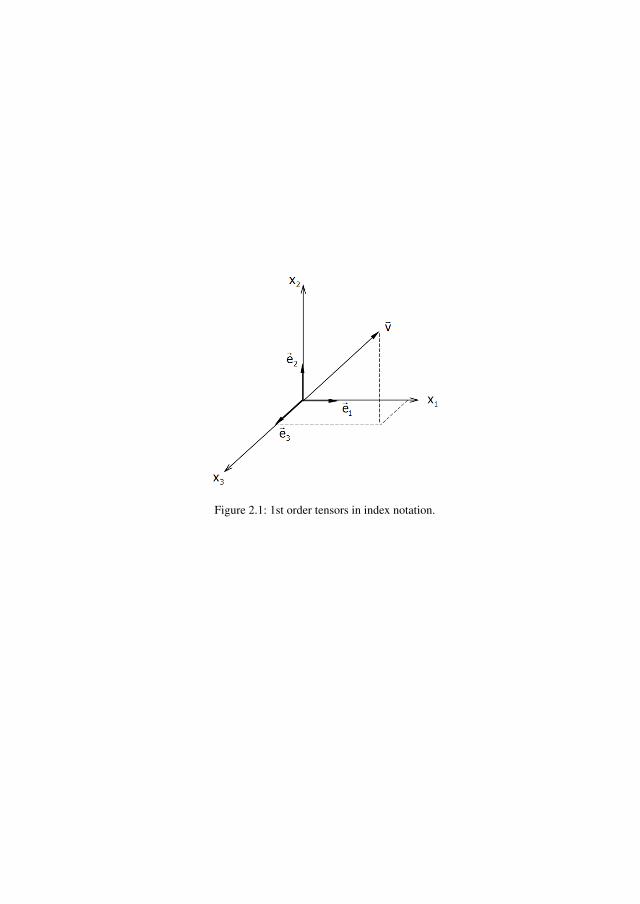
Figure 2.1: 1st order tensors in index notation.

V

�

2x

1x

2V

2e�

1e�

1V

2x

2V

2e�

1e� 1

V1

x

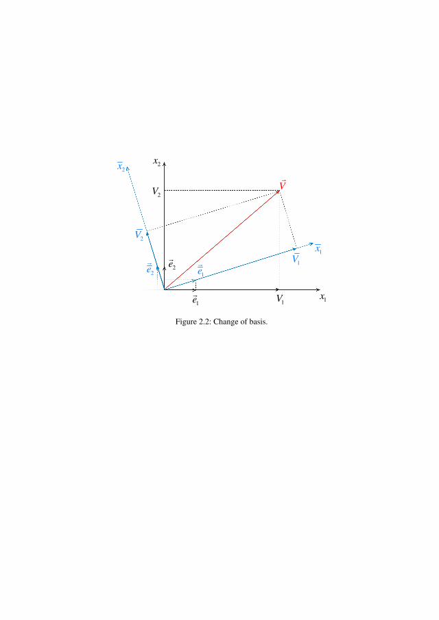
Figure 2.2: Change of basis.

33D

32D

31D

23D

22D

21D

13D

12D

11D

IIID

ID

IID

1e�

2e�

3e�

Ie�

IIe�

IIIe�

jQ

α

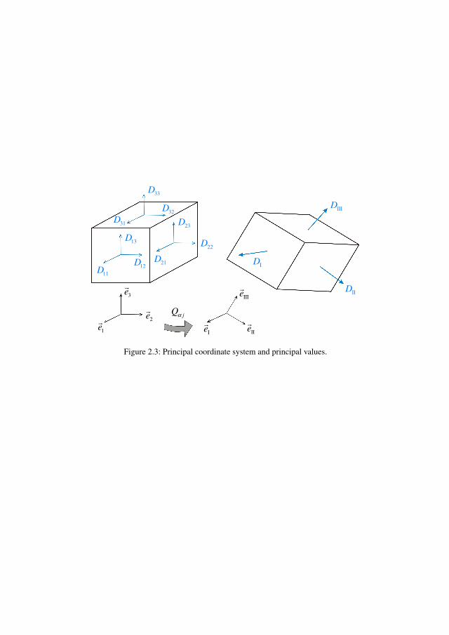
Figure 2.3: Principal coordinate system and principal values.

IIIe�

Ie�

IIe�

III

1

D

II

1

D

I

1

D

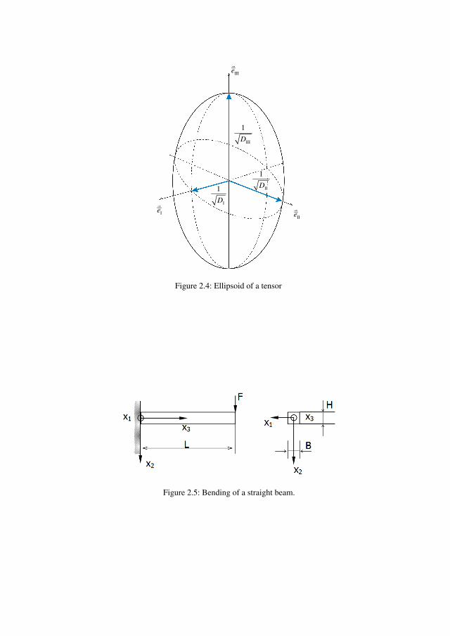
Figure 2.4: Ellipsoid of a tensor

Figure 2.5: Bending of a straight beam.

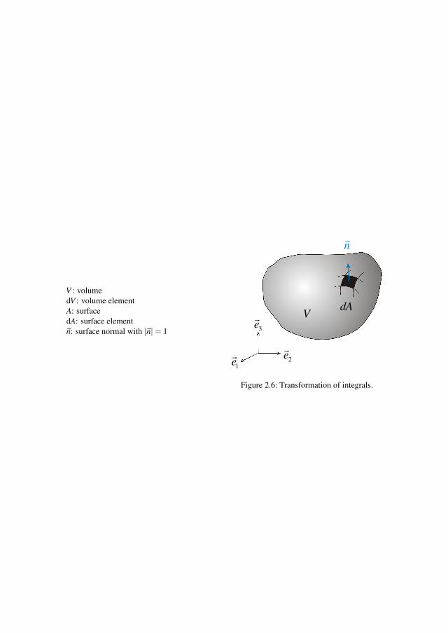
V : volumedV : volume elementA: surfacedA: surface element~n: surface normal with |~n|= 1

2e�

3e�

1e�

dAV

n�

Figure 2.6: Transformation of integrals.

1e�

2e�

3e�

x�

X

�

P

P’

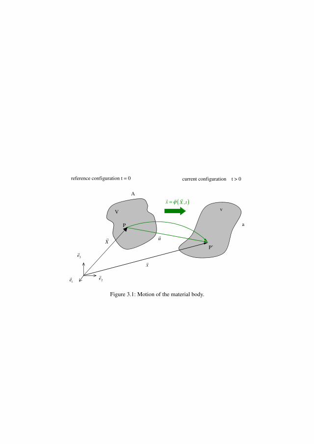
( ),x X tϕ=

���

u�

reference configuration t = 0 current configuration t > 0

V

A

v

a

Figure 3.1: Motion of the material body.

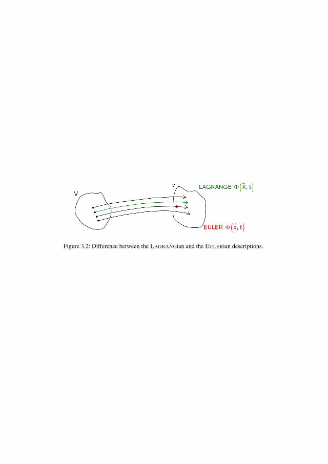
Figure 3.2: Difference between the LAGRANGian and the EULERian descriptions.

1e�

2e�

3e�

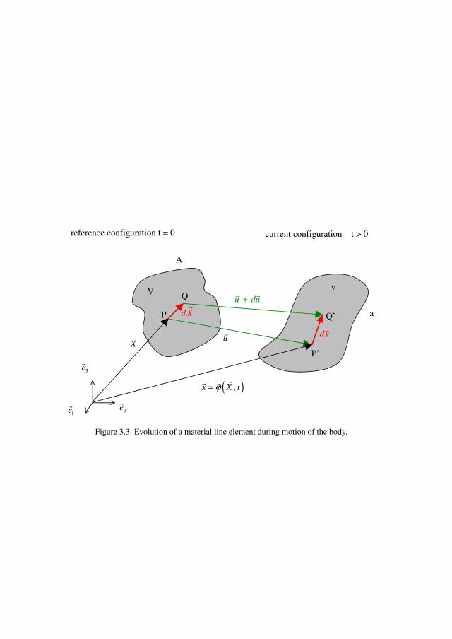
( ),x = X tϕ

�

��

X

�

P

P’

Q’

Q u du+� �

u� dx

�

d X

�

reference configuration t = 0 current configuration t > 0

V

A

v

a

Figure 3.3: Evolution of a material line element during motion of the body.

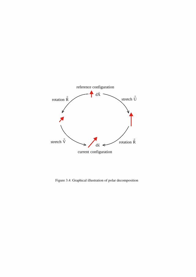
reference configuration

stretch U

rotation R

current configuration

stretch V

rotation R

dX

dx

Figure 3.4: Graphical illustration of polar decomposition

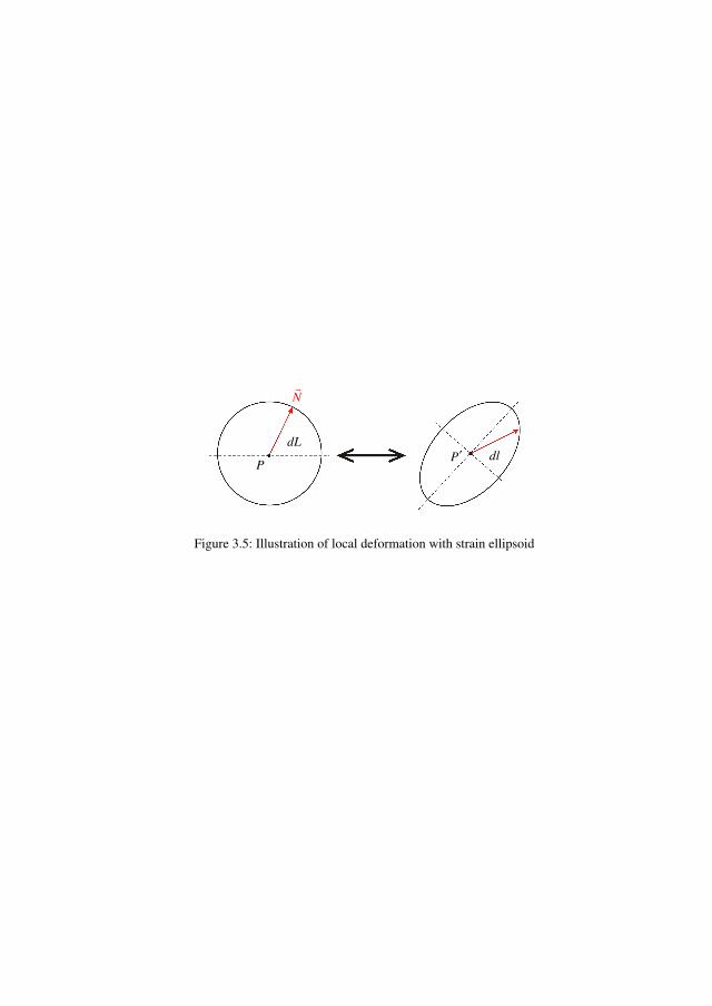
PP′

dL

dl

N

�

Figure 3.5: Illustration of local deformation with strain ellipsoid

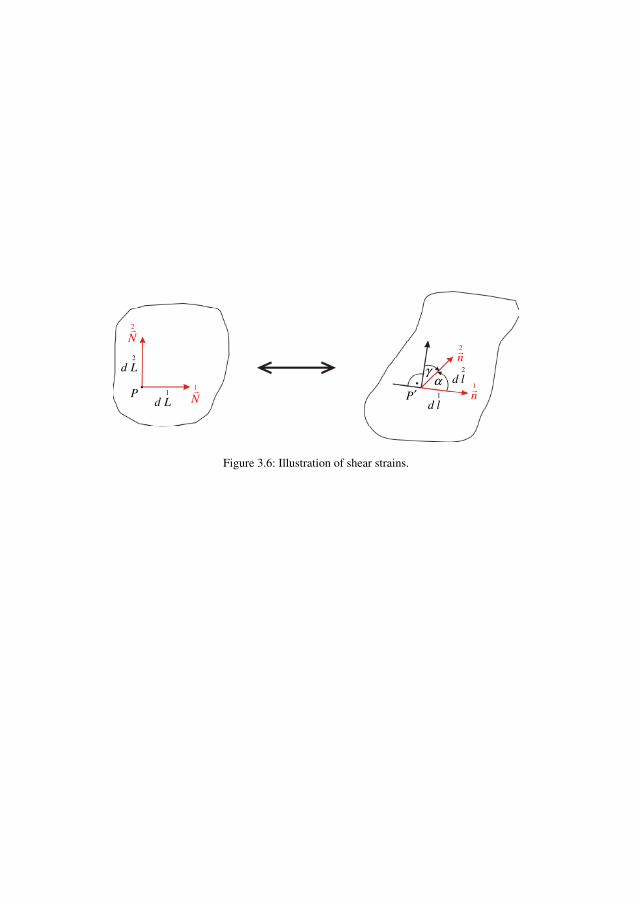
2

d L

1

d LP

2

N

�

1

N

�

2

n�

1

n�

P′ 1

d l

2

d lγ

α

Figure 3.6: Illustration of shear strains.

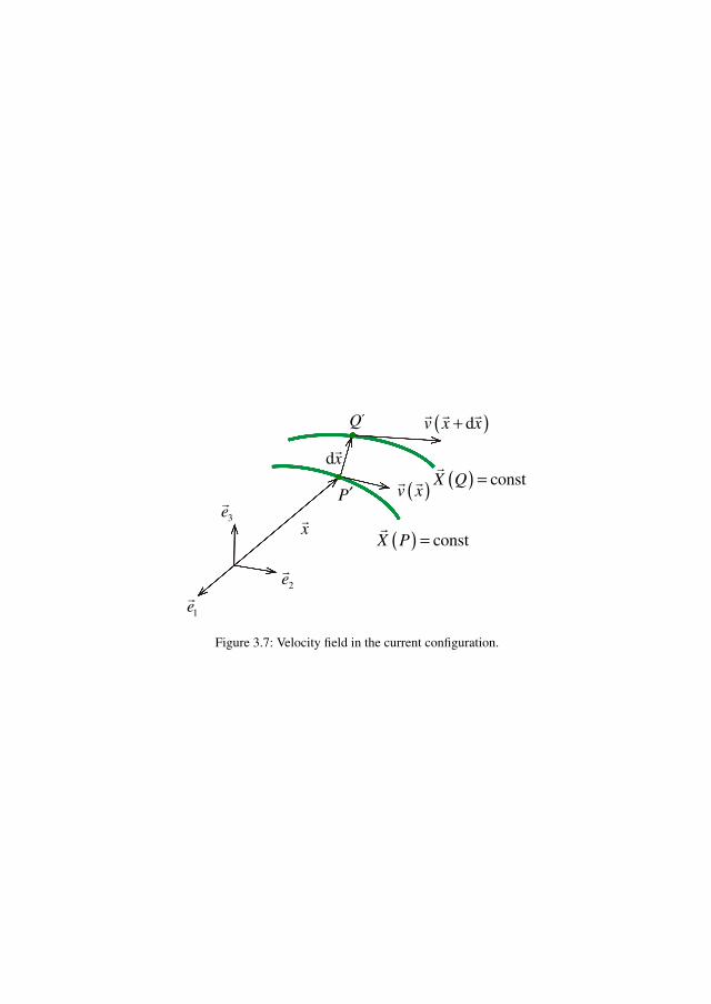
2e�

1e�

3e�

x�

dx�

′P

( ) constX P =

�

( )v x� � ( ) constX Q =

�

′Q ( )dv x x+� � �

Figure 3.7: Velocity field in the current configuration.

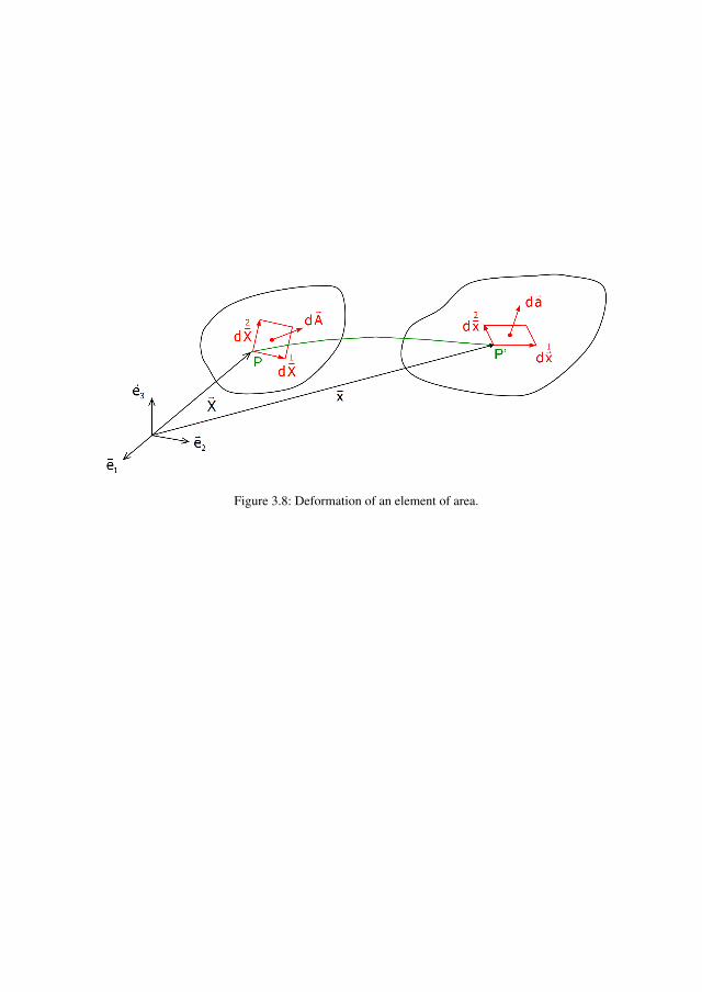
Figure 3.8: Deformation of an element of area.

d ,s t

d ,s b

dv

da

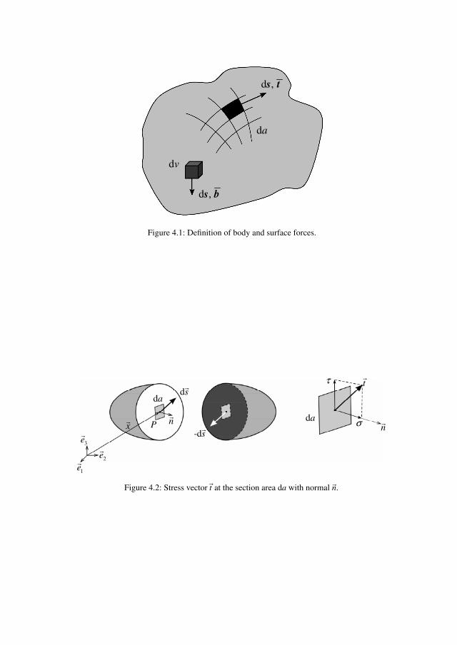
Figure 4.1: Definition of body and surface forces.

ds�

da

da

Pn�

n�

t�

3e�

1e�

2e�

x�

τ

σ

-ds�

Figure 4.2: Stress vector~t at the section area da with normal~n.

2x1

x

3x

31σ 32

σ

33σ

13σ

11σ

12σ

23σ

21σ

22σ

3t�

1t�

2t�

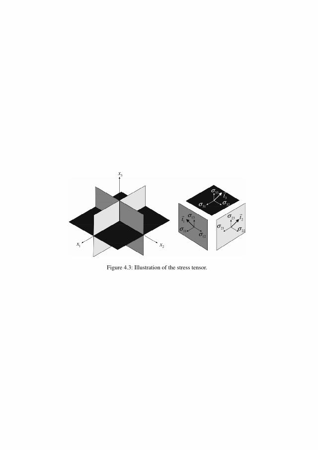
Figure 4.3: Illustration of the stress tensor.

2e�

1e�

e�

3

t�

t�

1

3t�

da

n�

da3

da2

da1

2t�

22σ

21σ

23σ

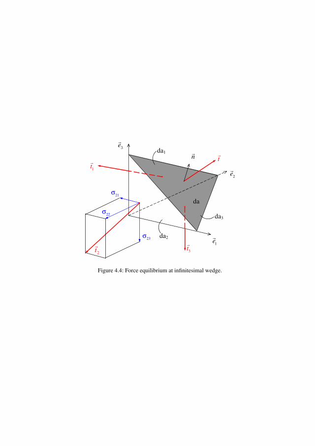
Figure 4.4: Force equilibrium at infinitesimal wedge.

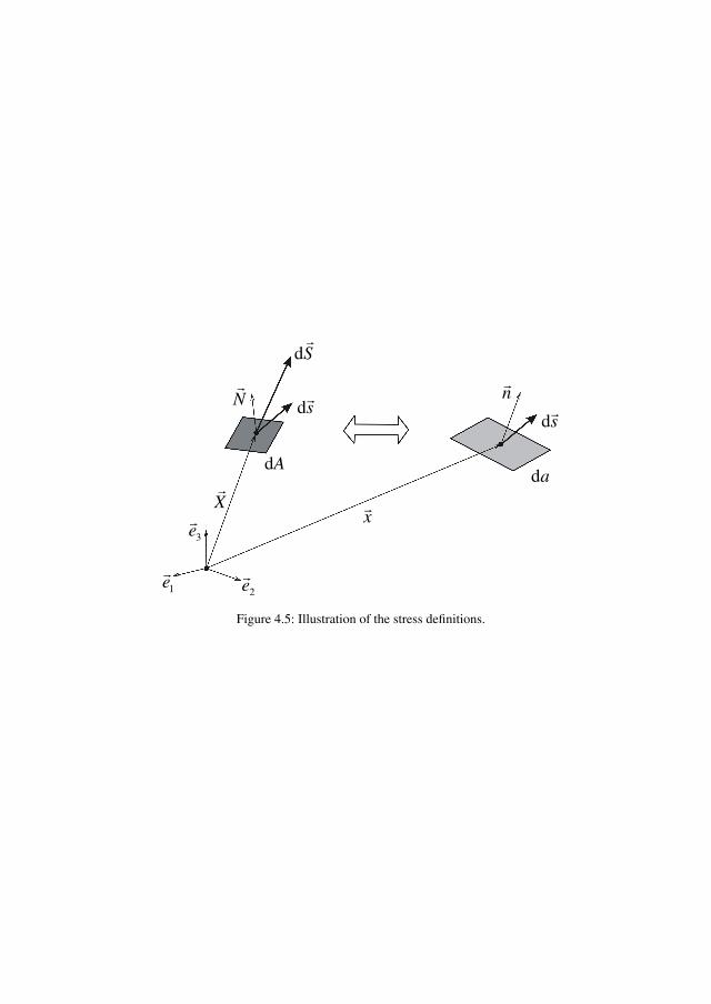
X

�

N

�

dS

�

ds�

dA

x�

n�

ds�

da

3e�

1e�

2e�

Figure 4.5: Illustration of the stress definitions.

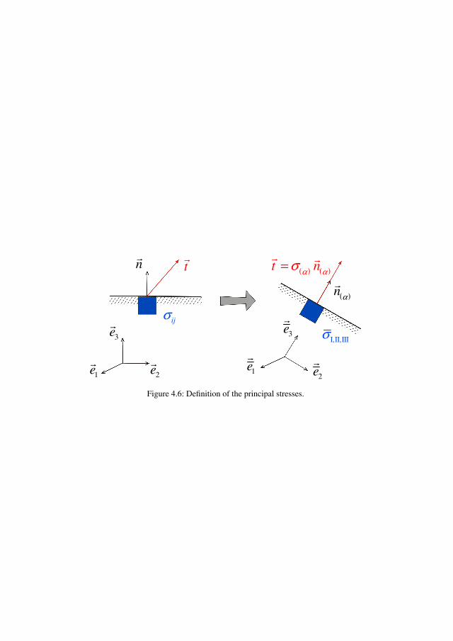
n�

( )n

α

�

1e�

2e�

3e�

1e�

2e�

3e�

t�

( ) ( )t n

α ασ=

��

ijσ

I,II,IIIσ

Figure 4.6: Definition of the principal stresses.

1e�

2e�

3e�

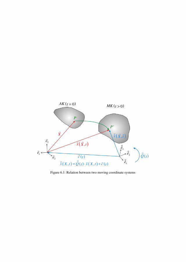
3e

�ɶ

2e

�ɶ

1e

�ɶ

( )0AK t =( )0MK t >

( )c t�

( ),x X t

� �ɶɶ

( )Q t

��

P

'P

X

�

( ),x X t

��

( ) ( ) ( ) ( ), ,x Q x cX t X tt t= ⋅ +

�� � � �ɶ

Figure 6.1: Relation between two moving coordinate systems

Figure 6.2: nonlinear-elastic constitutive law for rubber