MIT OpenCourseWare http://ocw.mit.edu Continuum Electromechanics For any use or distribution of this textbook, please cite as follows: Melcher, James R. Continuum Electromechanics. Cambridge, MA: MIT Press, 1981. Copyright Massachusetts Institute of Technology. ISBN: 9780262131650. Also available online from MIT OpenCourseWare at http://ocw.mit.edu (accessed MM DD, YYYY) under Creative Commons license Attribution-NonCommercial-Share Alike. For more information about citing these materials or our Terms of Use, visit: http://ocw.mit.edu/terms.

2

Electrodynamic Laws,Approximations and Relations

:14

2.1 Definitions

Continuum electromechanics brings together several disciplines, and so it is useful to summarizethe definitions of electrodynamic variables and their units. Rationalized MKS units are used not onlyin connection with electrodynamics, but also in dealing with subjects such as fluid mechanics and heattransfer, which are often treated in English units. Unless otherwise given, basic units of meters (m),kilograms (kg), seconds (sec), and Coulombs (C) can be assumed.

Table 2.1.1. Summary of electrodynamic nomenclature.

Name Symbol Units

Discrete Variables

Voltage or potential difference v [V] = volts = m2 kg/C sec2Charge q [C] = Coulombs = CCurrent i [A] = Amperes = C/secMagnetic flux X [Wb] = Weber = m2 kg/C secCapacitance C [F] = Farad C2 sec2 /m2 kgInductance L [H] = Henry = m2 kg/C2

Force f [N] = Newtons = kg m/sec2

Field Sources

Free charge density Pf C/m3

Free surface charge density •f C/m2

Free current density 4f A/m2

Free surface current density Kf A/m

Fields (name in quotes is often used for convenience)

"Electric field" intensity V/m"Magnetic field" intensity A/mElectric displacement C/m2

Magnetic flux density Wb/m 2 (tesla)Polarization density C/m2Magnetization density M A/mForce density F N/m3

Physical Constants

Permittivity of free space 6o = 8.854 x 1012 F/mPermeability of free space 1o = 4r x 10- 7 H/m

Although terms involving moving magnetized and polarized media may not be familiar, Maxwell'sequations are summarized without prelude in the next section. The physical significance of the un-familiar terms can best be discussed in Secs. 2.8 and 2.9 after the general laws are reduced to theirquasistatic forms, and this is the objective of Sec. 2.3. Except for introducing concepts concernedwith the description of continua, including integral theorems, in Secs. 2.4 and 2.6, and the dis-cussion of Fourier amplitudes in Sec. 2.15, the remainder of the chapter is a parallel development ofthe consequences of these quasistatic laws. That the field transformations (Sec. 2.5), integral laws(Sec. 2.7), splicing conditions (Sec. 2.10), and energy storages are derived from the fundamental quasi-static laws, illustrates the important dictum that internal consistency be maintained within the frame-work of the quasistatic approximation.

The results of the sections on energy storage are used in Chap. 3 for deducing the electric andmagnetic force densities on macroscopic media. The transfer relations of the last sections are animportant resource throughout all of the following chapters, and give the opportunity to explore thephysical significance of the quasistatic limits.

2.2 Differential Laws of Electrodynamics

In the Chu formulation,l with material effects on the fields accounted for by the magnetizationdensity M and the polarization density P and with the material velocity denoted by v, the laws ofelectrodynamics are:

Faraday's law

4+ 3H P-•at o M +(o Sto Bt

1. P. Penfield, Jr., and H. A. Haus, Electrodynamics of Moving Media, The M.I.T. Press, Cambridge,Massachusetts, 1967, pp. 35-40.

Ampere's law

V x H = E + + V x (P x v) + J (2)ot t f

Gauss' law

V*E = -V*P + Pf (3)

divergence law for magnetic fields

oV.H = -ioV *M (4)

and conservation of free charge

V'Jf + •t = 0 (5)

This last expression is imbedded in Ampere's and Gauss' laws, as can be seen by taking the diver-gence of÷-Eq. 2 and exploiting Eq. 3. In this formulation the electric displacement and magnetic fluxdensity B are defined fields:

D = E + P (6)o

4- -B = o(H + M) (7)

2.3 Quasistatic Laws and the Time-Rate Expansion

With a quasistatic model, it is recognized that relevant time rates of change are sufficientlylow that contributions due to a particular dynamical process are ignorable. The objective in thissection is to give some formal structure to the reasoning used to deduce the quasistatic field equa-tions from the more general Maxwell's equations. Here, quasistatics specifically means that timesof interest are long compared to the time, Tem, for an electromagnetic wave to propagate through thesystem.

Generally, given a dynamical process characterized by some time determined by the parameters ofthe system, a quasistatic model can be used to exploit the comparatively long time scale for proc-esses of interest. In this broad sense, quasistatic models abound and will be encountered in manyother contexts in the chapters that follow. Specific examples are:

(a) processes slow compared to wave transit times in general; acoustic waves and the model isone of incompressible flow, Alfvyn and other electromechanical waves and the model is less standard;

(b) processes slow compared to diffusion (instantaneous diffusion models). What diffuses canbe magnetic field, viscous stresses, heat, molecules or hybrid electromechanical effects;

(c) processes slow compared to relaxation of continua (instantaneous relaxation or constant-potential models). Charge relaxation is an important example.

The point of making a quasistatic approximation is often to focus attention on significantdynamical processes. A quasistatic model is by no means static. Because more than one rate processis often imbedded in a given physical system, it is important to agree upon the one with respect towhich the dynamics are quasistatic.

Rate processes other than those due to the transit time of electromagnetic waves enter throughthe dependence of the field sources on the fields and material motion. To have in view the additionalcharacteristic times typically brought in by the field sources, in this section the free currentdensity is postulated to have the dependence

Jf = G(r)E + Jv(v,pf,H) (i)

In the absence of motion, Jv is zero. Thus, for media at rest the conduction model is ohmic, with the

el-ctrical conductivity a in general a funqtion Qf position. Examples of Jv are a convection currentpfv, or an ohmic motion-induced current a(v x 0oH). With an underbar used to denote a normalizedquantity, the conductivity is normalized to a typical (constant) conductivity a :

a = (r,t) (2)o-

To identify the hierarchy of critical time-rate parameters, the general laws are normalized.Coordinates are normalized to one typical length X, while T represents a characteristic dynamical time:

(x,y,z) = (Zx,kY,kz); t = Tt (3)

Secs. 2.2 & 2.3

In a system sinusoidally excited at the angular frequency , T= W-1lIn a system sinusoidally excited at the angular frequency w, T=w

The most convenient normalization of the fields depends on the specific system. Where electro-mechanical coupling is significant, these can usually be categorized as "electric-field dominated" and"magnetic-field dominated." Anticipating this fact, two normalizations are now developed "in parallel,"the first taking e as a characteristic electric field and the second taking _ as.a characteristic mag-netic field:

o v T -v

p E f 80H 0 +pf =-9 , H=- - H,MM T-

H = H, M v = (/), = J

= Lf -v

E= P Pf p-,. P=f, - P

It might be appropriate with this step to recognize that the material motion introduces a characteristic(transport) time other than T. For simplicity, Eq. 4 takes the material velocity as being of the orderof R/T.

The normalization used is arbitrary. The same quasistatic laws will be deduced regardless of thestarting point, but the normalization will determine whether these laws are "zero-order" or higher orderin a sense to now be defined.

The normalizations of Eq. 4 introduced into Eqs. 2.2.1-5 result in

V.1 = -V.ý + pf

V.H = -V-M

+T +. + E 9P ( x)VxH = - aE + J + + -- +Vx (P xv)

T v +t ~te

H+ 3 xV

~-V]VxE = -s t t + Vx (x

Se F ~fV. E + - V*J t+ ]e v 't J

V.E = -V.p +

V.H = -V.M

Tm

VxH = -- ET

S HVxE = at

+ J + O +

V x (Mx v)

-ý T DpV. E + V + 0T T t =

m m

where underbars on equation numbers are used to indicate that the equations are normalized and

Tm 0a £ 2 , Te 0 0o/°

= -em Vo o£ = Z/c (10)

In Chap. 6, T will be identified as the magnetic diffusion time, while in Chap. 5 the role of the

charge-relaxation time Te is developed. The time required for an electromagnetic plane wave to propa-

gate the distance k at the velocity c is Tem. Given that there is just one characteristic length,there are actually only two characteristic times, because as can be seen from Eq. 10

(11)Tme em

Unless Te and Tm, and hence Tem, are all of the same order, there are only two possibilities for the

relative magnitudes of these times, as summarized in Fig. 2.3.1.

18W(II Ir

Tm •

electroquasistati cs

TCe mem

magnetoquasistatics

Fig. 2.3.1. Possible relations between physical time constants on a time

scale T which typifies the dynamics of interest.

Sec. 2.3

+ Vx(P x v (7)BtA

(8)

( 4((1 ~I _

By electroquasistatic (EQS) approximation it is meant that the ordering of times is as to the left andthat the parameter 08 (Tem/T)Z is much less than unity. Note that T is still arbitrary relative to Te.In the magnetoquasistatic (MQS) approximation, 0 is still small, but the ordering of characteristic timesis as to the right. In this case, T is arbitrary relative to Tm.

To make a formal statement of the procedure used to find the quasistatic approximation, the normal-ized fields and charge density are expanded in powers of the time-rate parameter 0.

E = E + E1 + E2+

0 0o+ H01+ 8 +2 (12)

iv - ( v)o + 0v) +0 ( )2 +

Pf = (Pf)o + (Pf) 1 + ()2 +

In the following, it is assumed that constitutive laws relate P and M to E and H, so that thesedensities are similarly expanded. The velocity 4 is taken as given. Then, the series are sub-stituted into Eqs. 5-9 and the resulting expressions arranged by factors multiplying ascendingpowers of 0. The "zero order" equations are obtained by requiring that the coefficients of 8vanish. These are simply Eqs. 5-9 with B = 0:

V.- o = -V.-P + (pf) o

VxHo = - o0

e

apo+ --- +

÷ at(Jv)o + --

Vx (o x V)

4.VxE 0

o

+ e • (v = 0V.oE +T- o + at

V.E = -V.o + (P)o

v-H -V-MT

VxH -- a E + (J )

aH aMVxE o Vx(M x V)

o at at 0

V.o E +_V.) =0Eo T V)om

The zero-order solutions are found by solving these equations, augmented by appropriate

boundary conditions. If the boundary conditions are themselves time dependent, normalization

will turn up additional characteristic times that must be fitted into the hierarchy of Fig. 2.3.1.

Higher order contributions to the series of Eq.

equations found by making coefficients of like powers

from setting the coefficients of an to zero are:

12 follow from a sequential solution of theof ý vanish. The expressions resulting

V En + V., - )n = 0

V*Fn+VM --0n - n Vn

e

at Vx (ýn x) = 0)

aM 1

atVx n ai Vx(Mi 1 x v)

V* Tn+ , n +I )a =o0n + ¶ )n at 0nl

V.* + ~*- (nf)nf = 0

v.* + V 0-n n

Vx. - mmE (J

V. E #n- E Tn tvnat nVAE ++x (mNO = 0

V T-C I a(Pf+(n T n atm m

(13)

(14)

(15)

(16)

(17)

-A

(18)

(19)

(20)

(21)

(22)

Sec. 2.3

To find the first order contributions, these equations with n=l are solved with the zero order

solutions making up the right-hand sides of the equations playing the role of known driving functions.

Boundary conditions are satisfied by the lowest order fields. Thus higher order fields satisfy homo-

geneous boundary conditions.Once the first order solutions are known, the process can be repeated with these forming the

"drives" for the n=2 equations.

In the absence of loss effects, there are no characteristic times to distinguish MQS and EQSsystems. In that limit, which set of normalizations is used is a matter of convenience. If a situa-tion represented by the left-hand set actually has an EQS limit, the zero order laws become the quasi-static laws. But, if these expressions are applied to a situation that is actually MQS, then first-order terms must be calculated to find the quasistatic fields. If more than the one characteristictime Tern is involved, as is the case with finite Te and Tm, then the ordering of rate parameters cancontribute to the convergence of the expansion.

In practice, a formal derivation of the quasistatic laws is seldom used. Rather, intuition andexperience along with comparison of critical time constants to relevant dynamical times is used toidentify one of the two sets of zero order expressions as appropriate. But, the use of normalizationsto identify critical parameters, and the notion that characteristic times can be used to unscrambledynamical processes, will be used extensively in the chapters to follow.

Within the framework of quasistatic electrodynamics, the unnormalized forms of Eqs. 13-17conmrise the "exact" field laws These enuations are reordered to reflect their relative imnortance:

Electroquasistatic (EQS)

V.-E E= -V'P + Pf

Vx = 0

S apfV.Jf + -ý-= 0

VxH = + +2-- + Vx (P x v)f t at

ViiH = -V PoM

Magnetoquasistatic (MQS)

Vx = f (23)

V.1oH = -V.o M (24)

a4,. allH 1VxE at at -oV x (M x v) (25)

V•J = o (26)

VeoE = -VP + Pf (27)0

The conduction current Jf has been reintroduced to reflect the wider range of validity of these

equations than might be inferred from Eq. 1. With different conduction models will come different

characteristic times,exemplified in the discussions of this section by Te and Tm. Matters are more

complicated if fields and media interact electromechanically. Then, v is determined to some extent

at least by the fields themselves and must be treated on a par with the field variables. The result

can be still more characteristic times.

The ordering of the quasistatic equations emphasizes the instantaneous relation between the

respective dominant sources and fields. Given the charge and polarization densities in the EQS system,

or given the current and magnetization densities in the MQS system, the dominant fields are known and

are functions only of the sources at the given instant in time.

The dynamics enter in the EQS system with conservation of charge, and in the MQS system with

Faraday'l law of induction. Equations 26a and 27a are only needed 4f an after-the-fact determina-tion of H is to be made. An example where such a rare interest in H exists is in the small mag-netic field induced by electric fields and currents within the human body. The distribution of in-

ternal fields and hence currents is determined by the first three EQS equations. Given 1, •, and

Jf, the remaining two expressions determine H. In the MQS system, Eq. 27b can be regarded as an

expression for the after-the-fact evaluation of pf, which is not usually of interest in such systems.

What makes the subject of quasistatics difficult to treat in a general way,even for a system

of fixed ohmic conductivity, is the dependence of the appropriate model on considerations not con-

veniently represented in the differential laws. For example, a pair of perfectly conducting plates,

shorted on one pair of edges and driven by a sinusoidal source at the opposite pair, will be MQS

at low frequencies. The same pair of plates, open-circuited rather than shorted, will be electroquasi-

static at low frequencies. The difference is in the boundary conditions.

Geometry and the inhomogeneity of the medium (insulators, perfect conductors and semiconductors)

are also essential to determining the appropriate approximation. Most systems require more than one

Sec. 2.3

characteristic dimension and perhaps conductivity for their description, with the result that more thantwo time constants are often involved. Thus, the two possibilities identified in Fig. 2.3.1 can inprinciple become many possibilities. Even so, for a wide range of practical problems, the appropriatefield laws are either clearly electroquasistatic or magnetoquasistatic.

Problems accompanying this section help to make the significance of the quasistatic limits moresubstantive by considering cases that can also be solved exactly.

2.4 Continuum Coordinates and the Convective Derivative

There are two commonly used representations of continuum variables. One of these is familiarfrom classical mechanics, while the other is universally used in electrodynamics. Because electro-mechanics involves both of these subjects, attention is now drawn to the salient features of the tworepresentations.

Consider first the "Lagrangian representation." The position of a material particle is a naturalexample and is depicted by Fig. 2.4.1a. When the time t is zero, a particle is found at the positionro . The position of the particle at some subsequent time is t. To let t represent the displacement ofa continuum of particles, the position variable ro is used to distinguish particles. In this sense, thedisplacement ý then also becomes a continuum variable capable of representing the relative displace-ments of an infinitude of particles.

u) kU)Fig. 2.4.1. Particle motions represented in terms of (a) Lagrangian coordinates,

where the initial particle coordinate ro designates the particle ofinterest, and (b) Eulerian coordinates, where (x,y,z) designates thespatial position of interest.

In a Lagrangian representation, the velocity of the particle is simply

at

If concern is with only one particle, there is no point in writing the derivative as a partial deriv-ative. However, it is understood that, when the derivgtive is taken, it is a particular particlewhich is being considered. So, it is understood that ro is fixed. Using the same line of reasoning,the acceleration of a particle is given by

a at

The idea of representing continuum variables in terms of the coordinates (x,y,z) connected withthe space itself is familiar from electromagnetic theory. But what does it mean if the variable ismechanical rather than electrical? We could represent the velocit- of the continuum of particlesfilling the space of interest by a vector function v(x,y,z,t) = v(r,t). The velocity of particles

having the position (x,y,z,) at a given time t is determined by evaluating the function v(r,t). Thevelocity appearing in Sec. 2.2 is an example. As suggested by Fig. 2.4.1b, if the function is the

velocity evaluated at a given position in space, it describes whichever particle is at that point at

the time of interest. Generally, there is a continuous stream of particles through the point (x,y,z).

Secs. 2.3 & 2.4

~

)

Computation of the particle acceleration makes evident the contrast between Eulerian and Lagrangianrepresentations. By definition, the acceleration is the rate of change of the velocity computed for agiven particle of matter. A particle having the position (x,y,z) at time t will be found an instantAt later at the position (x + vxAt,y + vyAt,z + vzAt). Hence the acceleration is

v(x + v At,y + v At,z + v At,t + At) - v(x,y,z,t)a=lim x y z (3)

At÷OAt

Expansion of tje first term in Eq. 3 about the initial coordinates of the particle gives the convectivederivative of v:

+ v av av av _ v + +a + v + v + v + v*Vv (4)

t x ax y y z (4)at

The difference between Eq. 2 and Eq. 4 is resolved by recognizing the difference in the signi-ficance of the partial derivatives. In Eq. 2, it is understood that the coordinates being held fixedare the initial coordinates of the particle of interest. In Eq. 4, the partial derivative is taken,holding fixed the particular point of interest in space.

The same steps .show that the rate of change of any vector variable A, as viewed from a particlehaving the velocity v, is

DAaA 31 + (S- + (V); A = A(x,y,z,t) (5)

The time rate of change of any scalar variable for an observer moving with the velocity v is obtainedfrom Eq. 5 by considering the particular case in which t has only one component, say 1 = f(x,y,z,t)Ax.Then Eq. 5 becomes

Df f +ff- E - -+ v.Vf (6)

Reference 3 of Appendix C is a film useful in understanding this section.

2.5 Transformations between Inertial Frames

In extending empirically determined conduction, polarization and magnetization laws to includematerial motion, it is often necessary to relate field variables evaluated in different referenceframes. A given point in space can be designated either in terms of the coordinate 1 or of the co-ordinate V' of Fig. 2.5.1. By "inertial reference frames," it is meant that the relative velocitybetween these two frames is constant, designated by '. The positions in the two coordinate systemsare related by the Galilean transformation:

r' = r - ut; t' = t (1)

Fig. 2.5.1

Reference frames have constantrelative velocity t. The co-ordinates t = (x,y,z) and 1' =(x',y',z') designate the sameposition.

It is a familiar fact that variables describing a given physical situation in one reference framewill not be the same as those in the other. An example is material velocity, which, if measured in oneframe, will differ from that in the other frame by the relative velocity ~.

There are two objectives in this section: one is to show that the quasistatic laws are invariantwhen subject to a Galilean transformation between inertial reference frames. But, of more use is the

relationship between electromagnetic variables in the two frames of reference that follows from this

Secs. 2.4 & 2.5

proof. The approach is as follows. First, the postulate is made that the quasistatic equations take the

same form in the primed and unprimed inertial reference frames. But, in writing the laws in the primed

frame, the spatial and temporal derivatives must be taken with respect to the coordinates of that ref-

erence frame, and the dependent field variables are then fields defined in that reference frame. In

general, these must be designated by primes, since their relation to the variables in the unprimed frame

is not known.

For the purpose of writing the primed equations of electrodynamics in terms of the un rimed co-Forthe nurnose o writina the nrimd enuations of elctrod-ax cs in tems of the u- rimeordinates, recognize that

V' + V

A a )+ - = al"a-)+ (- + u*V)A - + uV*A - Vx (uxA)

+(+ uV9 +Vu( t + E at

The left relations follow by using the chain rule of differentiation and the transformation of Eq. 1.That the spatial derivatives taken with respect to one frame must be the same as those with respectto the other frame physically means that a single "snapshot" of the physical process would be allrequired to evaluate the spatial derivatives in either frame. There would be no way of telling whichframe was the one from which the snapshot was taken. By contrast, the time rate of change for anobserver in the primed frame is, by definition, taken with the primed spatial coordinates held fixed.In terms of the fixed frame coordinates, this is the convective derivative defined with Eqs. 2.4.5and 2.4.6. However, v in these equations is in general a function of space and time. In the contextof this section it is saecialized to the constant u. Thus, in rewriting the convective derivatives ofEq. 2 the constancy of u and a vector identity (Eq. 16, Appendix B) have been used.

So far, what has been said in this section is a matter of coordinates. Now, a physically motivatedpostulate is made concerning the electromagnetic laws. Imagine one electromagnetic experiment that isto be described from the two different reference frames. The postulate is that provided each of theseframes is inertial, the governing laws must take the same form. Thus, Eqs. 23-27 apply with [V - V',c()/at - a()/at'] and all dependent variables primed. By way of comparing these laws to those ex-

pressed in the fixed-frame, Eqs. 2 are used to rewrite these expressions in terms of the unprimed in-dependent variables. Also, the moving-frame material velocity is rewritten in terms of the unprimedframe velocity using the relation

v' v- u

Thus, the laws originally expressed in the primed frame of reference become

V.e E'E -V.P' + p0 f

V x E' = 0

V.(ij + up!) + - 0

V x (' + ux C ') - ( + up )

aE$' + ' x,+ + + V x (P xat at

V~o oM0

V x i' =

V*oH' -V.o0 M'

Vx(' - u x ~i')al H0'at

ay M'- (6)at

- V x (' x V)

- f

V~eo'= V.P'+ !

In writing Eq. 7a, Eq. 4a is used. Similarly, Eq. 5b is used to write Eq. 6b. For the one experi-ment under consideration, these equations will.predict the same behavior as the fixed frame laws,Eqs. 2.3.23-27, if the identification is made:

Sec. 2.5

E- ,

PE'= P

4. 4 +

S= J -Upf

H' .'A-i x eEo

and hence, from Eq. 2.2.6

D' =D

MQS

'- A (9)4. +M' = M (10)

J = Jf (11)

E'= E + ux poH (12)

(13)

and hence, from Eq. 2.2.7

B' = B (14)

The primary fields are the same whether viewed from one frame or the other. Thus, the EQS elec-tric field polarization density and charge density are the same in both frames, as are the MQS mag-netic field, magnetization density and current density. The respective dynamic laws can be associatedwith those field transformations that involve the relative velocity. That the free current densityis altered by the relative motion of the net free charge in the EQS system is not surprising. But, itis the contribution of this same convection current to Ampere's law that generates the velocity depend-ent contribution to the EQS magnetic field measured in the moving frame of reference. Similarly, thevelocity dependent contribution to the MQS electric field transformation is a direct consequence ofFaraday's law.

The transformations, like the quasistatic laws from which they originate, are approximate. Itwould require Lorentz transformations to carry out a similar procedure for the exact electrodynamiclaws of Sec. 2.2. The general laws are not invariant in form to a Galilean transformation, and there-in is the origin of special relativity. Built in from the start in the quasistatic field laws is aself-consistency with other Galilean invariant laws describing mechanical continua that will be broughtin in later chapters.

2.6 Integral Theorems

Several integral theorems prove useful, not only in the description of electromagnetic fields butalso in dealing with continuum mechanics and electromechanics. These theorems will be stated here with-out proof.

If it is recognized that the gradient operator is defined such that its line integral between twoendpoints (a) and (b) is simply the scalar function evaluated at the endpoints, thenl

I w4= -M) (1)a

Two more familiar theorems1 are useful in dealing with vector functions. For a closed surface S, en-closing the volume V, Gauss' theorem states that

V*AdV = '-nda (2)V S

while Stokes's theorem pertains to an open surface S with the contour C as its periphery:

SV x A•1da = A' (3)S C

In stating these theorems, the normal vector is defined as being outward from the enclosed voluge forGauss' theorem, and the contour is taken as positive in a direction such that It is related to n by theright-hand rule. Contours, surfaces, and volumes are sketched in Fig. 2.6.1.

A possibly less familiar theorem is the generalized Leibnitz rule.2 In those cases where thesurface is itself a function of time, it tells how to take the derivative with respect to time of theintegral over an open surface of a vector function:

1. Markus Zahn, Electromagnetic Field Theory, a problem solving approach, John Wiley & Sons, New York,1979, pp. 18-36.

2. H. H. Woodson and J. R. Melcher, Electromechanical Dynamics, Vol. 1. John Wiley & Sons, New York,1968, pp. B32-B36.(See Prob. 2.6.2 for the derivation of this theorem.)

Secs. 2.5 & 2.6

(a) (b) (c)Fig. 2.6.1. Arbitrary contours, volumes and surfaces: (a) open contour C;

(b) closed surface S, enclosing volume V; (c) open surface Swith boundary contour C.

- A~nda = [ + (V.A)v ]-nda + (IAx ).dx (4)dt at sS S C

Again, C is the contour which is the periphery of the open surface S. The velocity vs is the velocityof the surface and the contour. Unless given a physical significance, its meaning is purely geometrical.

A limiting form of the generalized Leibnitz rule will be handy in dealing with closed surfaces.Let the contour C of Eq. 4 shrink to zero, so that the surface S becomes a closed one. This process canbe readily visualized in terms of the surface and contour sketch in Fig. 2.6.1c if the contour C ispictured as the draw-string on a bag. Then, if C V-1, and use is made of Gauss' theorem (Eq. 2),Eq. 4 becomes a statement of how to take the time derivative of a volume integral when the volume is afunction of time:

dV = f dV + s.nda (5)tV Vt S

Again, vs is the velocity of the surface enclosing the volume V.

2.7 quasistatic Integral Laws

There are at least three reasons for desiring Maxwell's equations in integral form. First, theintegral equations are convenient for establishing jump conditions implied by the differentialequations. Second, they are the basis for defining lumped parameter variables such as the voltage,charge, current, and flux. Third, they are useful in understanding (as opposed to predicting) physicalprocesses. Since Maxwell's equations have already been divided into the two quasistatic systems, itis now possible to proceed in a straightforward way to write the integral laws for contours, surfaces,and volumes which are distorting, i.e., that are functions of time. The velocity of a surface S is v .

To obtain the integral laws implied by the laws of Eqs. 2.3.23-27, each equation is either(i) integrated over an open surface S with Stokes's theorem used where the integrand is a curl operatorto convert to a line integration on C and Eq. 2.6.4 used to bring the time derivative outside theintegral, or (ii) integrated over a closed volume V with Gauss' theorem used to convert integrationsof a divergence operator to integrals over closed surfaces S and Eq. 2.6.5 used to bring the timederivative outside the integration:

(E(E + P).-da = fdVS V

Jnda I fdV = 0

S V

H. = IJf da (1)C S

110 (H + M).nda - 0 (2)S

. -o(H + M)*nda (3)C S

- OPM x (:v- ).h%C

Secs. 2.6 & 2.7 2.10

H1.£ = J i.nda + (eE + P).n'daC S S

+ F P x (v - ')*C

SJo(H + M)-nda = 0S

where

J• J - VsPf+ 4 4..H' =H - v x sE

s o

Sf.-nda = 0S

+ P).nda = PfdVV

where4' -E+ s

x.

E' -E+v xIIH0

The primed variables are simply summaries of the variables found in deducing these equations. However,these definitions are consistent with the transform relationships found in Sec. 2.5, and the velocityof these surfaces and contours, vs, can be identified with the velocity of an inertial frame instan-taneously attached to the surface or contour at the point in question. Approximations implicit to theoriginal differential quasistatic laws are now implicit to these integral laws.

2.8 Polarization of Moving Media

Effects of polarization and magnetization are included in the formulation of electrodynamicspostulated in Sec. 2.2. In this and the next section a review is made of the underlying models.

Consider the electroquasistatic systems, where the dominant field source is the charge density.Not all of this charge is externally accessible, in the sense that it cannot all be brought to someposition through a conduction process. If an initially neutral dielectric medium is stressed by anelectric field, the constituent molecules and domains become polarized. Even though the materialretains its charge neutrality, there can be a local accrual or loss of charge because of the polariza-tion. The first order of business is to deduce the relation of such polarization charge to the polari-zation density.

For conceptual purposes, the polarization of a material is pictured as shown in Fig. 2.8.1.

Fig. 2.8.1. Model for dipoles fixed to deformable material. The model picturesthe negative charges as fixed to the material, and then the positivehalves of the dipoles fixed to the negative charges through internalconstraints.

Secs. 2.7 & 2.82.11

Fig. 2.8.2

Polarization results in netcharges passing through asurface.

The molecules or domains are represented by dipoles composed of positive and negative charges +q,separated by the vector distance 1. The dipole moment is then $ = qp, and if the particles have anumber density n, the polarization density is defined as

P = nqa (1)

In the most common dielectrics, the polarization results because of the application of an externalelectric field. In that case, the internal constraints (represented by the springs in Fig. 2.8.1)make the charges essentially coincident in the absence of an electric field, so that, on the average,the material is (macroscopically) neutral. Then,.with the application of the electric field, thereis a separation of the charges in some direction which might be coincident with the applied electricfield intensity. The effect of the dipoles on the average electric field distribution is equivalentto that of the medium they model.

To see how the polarization charge density is related to the polarization density, consider themotion of charges through the arbitrary surface S shown in Fig. 2.8.2. For the moment, consider thesurface as being closed, so that the contour enclosing the surface shown is shrunk to zero. Becausepolarization results in motion of the positive charge, leaving behind the negative image charge, the netpolarization charge within the volume V enclosed by the surface S is equal to the negative of the netcharge having left the volume across the surface S. Thus,

f pdV = - nq.i~da = - *"-da (2)P J J

S S

Gauss' theorem, Eq. 2.6.2, converts the surface integral to one over the arbitrary volume V. Itfollows that the integrand must vanish so that

4.

p = - V.P (3)

This polarization charge density is now added to the free charge density as a source of the electricfield intensity in Gauss' law:

V.E = Pf +Pp (4)

and Eqs. 3 and 4 comprise the postulated form of Gauss' law, Eq. 2.3.23a.

By definition, polarization charge is conserved, independent of the free charge. Hence, thepolarization current I is defined such that it satisfies the conservation equation

p

appV*J + at-= 0 (5)p at

To establish the way in which J transforms between inertial reference frames, observe that in a primedframe of reference, by dint of Eq. 2.5.2c, the conservation of polarization charge equation becomes

Bap'V. [, + up'] + L= 0 (6)

It has been shown that P, and hence pp, are the same in both frames (Eq. 2.5.10a). It follows that therequired transformation law is

SJ - up (7)p p p

If the dipoles are attached to a moving medium, so that the negative charges move with the samevelocity l as the moving material, the motion gives rise to a current which should be included inAmpere's law as a source of magnetic field. Even if the material is fixed, but the applied field is

Sec. 2.8 2.12

time-varying so as to induce a time-varying polarization density, a given surface is crossed by a netcharge and there is a current caused by a time-varying polarization density. The following stepsdetermine the current density 1p in terms of the polarization density and the material velocity.

The starting point is the statement

S-nda = P.nda (8)P ddt f

S S

The surface S, depicted by Fig. 2.8.2, is attached to the material itself. It moves with thenegative charges of the dipoles. Integrated over this deforming surface of fixed identity, the polari-zation current density evaluated in the frame of reference of the material is equal to the rate ofchange with respect to time of the net charge penetrating that surface.

With the surface velocity identified with the material velocity, Eq. 2.6.4 and Eq. 3 convertEq. 8 to

ap+4af t P + f ' x v. (9)S S 4On the left, J' is replaced by Eq. 7 evaluated with u = v, while on the right Stokes's theorem,Eq. 2.6.3, is Rsed to convert the line integral to a surface integral. The result is an equation insurface integrals alone. Although fixed to the deforming material, the surface S is otherwise arbitraryand so it follows that the required relation between 3p and I for the moving material is

+ 1P+10J = + V x(P ) (10)p at

It is this current density that has been added to the right-hand side of Ampere's law, Eq. 2.3.26a,to complete the formulation of polarization effects in the electroquasistatic system.

2.9 Magnetization of Moving Media

It is natural to use polarization charge to represent the effect of macroscopic media on themacroscopic electric field. Actually, this is one of two alternatives for representing polarization.That such a choice has been made becomes clear when the analogous question is asked for magnetization.In the absence of magnetization, the free current density is the source of the magnetic field, and itis therefore natural to represent the macroscopic effects of magnetizable media on ý through an equi-valent magnetization current density. Indeed, this viewpoint is often used and supported by the con-tention that what is modeled at the atomic level is really a system of currents (the electrons in theirorbits). It is important to understand that the use of equivalent currents, or of equivalent magneticcharge as used here, if carried out self-consistently, results in the same predictions of physicalprocesses. The choice of models in no way hinges on the microscopic processes accounting for the mag-netization. Moreover, the magnetization is often dominated by dynamical processes that have more to dowith the behavior of domains than with individual atoms, and these are most realistically pictured assmall magnets (dipoles). With the Chu formulation postulated in Sec. 2.2, the dipole model forrepresenting magnetization has been adopted.

An advantage of the Chu formulation is that magnetization is developed in analogy to polarization.But rather than starting with a magnetic charge density, and deducing its relation to the polarizationdensity, think of the magnetic material as influencing the macroscopic fields through an intrinsic fluxdensity poi that might be given, or might be itself induced by the macroscopic A. For lack of evidenceto support the existence of "free" magnetic monopoles, the total flux density due to all macroscopicfields must be solenoidal. Hence, the intrinsic flux density 'o40 , added to the flux density in freespace Plo, must have no divergence:

V.*o(, + M) = 0 (1)

This is Eq. 2.3.24b. It is profitable to think of -V.poM as a source of H. That is, Eq. 1 canbe written to make it look like Gauss' law for the electric field:

V H4H= pm; Pm = -V'Vo0 (2)

The magnetic charge density pm is in this sense the source of the magnetic field intensity.

Faraday's law of induction must be revised if magnetization is present. If o-M is a magnetic flux

density, then, through magnetic induction, its rate of change is capable of producing an induced electric

field intensity. Also, if Faraday's law of induction were to remain valid without alteration, then its

divergence must be consistent with Eq. 1; obviously, it is not.

Secs. 2.8 & 2.92.13

To generalize the law of induction to include magnetization, it is stated in integral form for acontour C enclosing a surface S fixed to the material in which the magnetized entities are imbedded.Then, because 1o(A + M) is the total flux density,

=E'*£= - d O(H + M)*nda

The electric field E' is evaluated in the frame of reference of the moving contour. With the timederivative taken inside the temporally varying surface integrals (Eq. 2.6.4) and because of Eq. 1,

C(t( + M)]*nda + xV x (x+ M)]*nda

S

44.The transformation law for E (Eq. 2.5.12b with u = v) is now used to evaluate E', and Stokes's theorem,Eq. 2.6.3, used to convert the line integral to a surface integral. Because S is arbitrary, it thenfollows that the integrand must vanish:

V-xE ((H+ M)) ] + V x (vx oPM)

This generalization of Faraday's law is the postulated equation, Eq. 2.3.25b.

2.10 Jump Conditions

Systems having nonuniform properties are often modeled by regions of uniform properties, separatedby boundaries across which these properties change abruptly. Fields are similarly often given a piece-wise representation with jump conditions used to "splice" them together at the discontinuities. Theseconditions, derived here for reference, are implied by the integral laws. They guarantee that theassociated differential laws are satisfied through the singular region of the discontinuity.

A 71

Fig. 2.10.1. Volume element enclosing a boundary. Dimen-sions of area A are much greater than A.

Electroquasistatic Jump Conditions: A section of the boundary can be enclosed by a volume elementhaving the thickness A and cross-sectional area A, as depicted by Fig. 2.10.1. The linear dimensions ofthe cross-sectional area A are, by definition, much greater than the thickness A. Implicit to thisstatement is the assumption that, although the surface can be curvilinear, its radius of curvature mustbe much greater than a characteristic thickness over which variations in the properties and fields takeplace.

The normal vector n used in this section is a unit vector perpendicular to the boundary and directifrom region b to region a, as.shown in Fig. 2.10.1. Since this same symbol is used in connection withintegral theorems and laws to denote a normal vector to surfaces of integration, these latter vectorsare denoted by 1 .

n

First, consider the boundary conditions implied by Gauss' law, Eq. 2.3.23a, with Eq. 2.8.3 used to

introduce pp. This law is first multiplied by vm and then integrated over the volume V:

Secs. 2.9 & 2.10 2.14

vm V oEdV mpfdV

V V

+ f VmpdV

V

Here, v is a coordinate (like x,y, or z) perpendicular to the boundary and hence in the direction of n,as shown in Fig. 2.10.1.

First, consider the particular case of Eq. 1 with m = 0. Then, the integration gives

n* EE J = af + ap

where 1 AII- b and L -P a - b and thecharge density ap have been defined as

f = lim f pfdV,A+o

free surface charge density Of and polarization surface

S= lim1 PpdVA-p T f0

The relationship between the surface charge andcan be pictured as shown in Fig. 2.10.2b.

V

the electric field intensity normal to the boundary

V V

-A/2 A/2 -A/2 A/2

1'

(a)

-A/2 A/2

tV

(b) (c)

Fig. 2.10.2. Sketches of the charge distribution represented by the solid lines, and theelectric field intensity normal to the boundary represented by broken lines.Sketches at the top represent actual distributions, while those below re-present idealizations appropriate if the thickness A of the region over whichthe electric field intensity makes its transition is small compared to otherdimensions of interest: (a) volume charge density to either side of inter-face but no surface charge; (b) surface charge; (c) double layer.

In view of Eq. 2, the normal electric field intensity is continuous at the interface unless thereis a singularity in charge. Thus, with volume charges to either side of the interface, there is anabrupt change in the rate of change of the electric field intensity normal to the boundary, but thefield is itself continuous. On the other hand, as illustrated by the sketches of Fig. 2.10.2b, if

there is an appreciable charge per unit area within the boundary, the electric field intensity is

discontinuous, and undergoes a step discontinuity.

Sec. 2.10

V1_______,

2.15

A somewhat less familiar situation is that of Fig. 2.10.2c. Within the boundary there areregions of large positive and negative charge concentrations with an associated intense electric fieldbetween. In the limit where the boundary becomes very thin, a component of the surface charge densitybecomes a doublet, and the electric field becomes an impulse.

The double layer can be pictured as being positive surface charges disposed on one side of theboundary, and negative surface charges distributed on the other, with an internal component of theelectric field originating on the positive charges and terminating on the negative ones. The mag-nitude of the double layer is equal to the product of the positive surface charge density and the dis-tance between these layers, A. In the limit where the layer thickness becomes infinitely thin while thedouble-layer magnitude remains constant, the electric field within the double layer must approachinfinity. Thus, associated with the doublet of charge density, there is an impulse in the electric fieldintensity, as sketched in Fig. 2.10.2c.

The boundary condition to be used in connection with a double layer is found from Eq. 1 by lettingm = 1. The left-hand side of Eq. 1 can be integrated by parts, so that it becomes

f V.(EoV )dV - f E.*VvdV = V(pf + p )dV (4)

V V V

For the incremental volume, the surface double layer density is defined as

p lim 1 f v(pf + pp)dV = v(p + p )dv (5)

and so the right-hand side of Eq. 4 is ApE. The origin of the A axis remains to be defined but A v -vTo glean a jump condition from the equation, the second EQS law is incorporated. That I is irrotational,Eq. 2.3.24a, is represented by defining the electric potential

E = -VO (6)

Thus, the second term on the left in Eq. 4 becomes

Je E*VvdV = - VO*VvdV = - f V*(OVv)dV + fE V2vdV (7)

V V V V

Evaluation of V2v gives nothing because v is defined as a local Cartesian coordinate. The last inte-gral vanishes, and with the application of Gauss' theorem, Eq. 2.6.2, it follows that Eq. 4 becomes

r V-.t da + f e IVv.i da - Ap (8)So n o n AS S

Provided that within the layer, E parallel to the interface and Q are finite (not impulses in the limitA÷0), Eq. 8 only has contributions to the surface integrals from the regions to either side of the inter-face. Thus,

AEo(vEa - v Eb). + Ae 0 = A pE (9)

The origin of the v axis is adjusted to make the first term vanish. The required boundary conditionto be associated with Eqs. 2.3.23a and 2.3.23b is

o II D= EP (10)

The gradient of Eq. 10 within the plane of the interface converts the jump condition to one in

terms of the electric field:

Eo a ID - VEZE (11)

Here VE is the surface gradient and t denotes components tangential to the interfacial plane.

In the absence of a double-layer surface density, these last two boundary conditions are thefamiliar statement that the tangential electric field intensity at a boundary must be continous. Thestatement given in Eq. 10 that the potential must be continuous at a boundary is another way of stating

Sec. 2.10 2.16

S 2.10

this requirement on the tangential electric field intensity. With a double layer, the tangential elec-tric field intensity is discontinuous, as is also the potential.

Equations 10 and 11 could also be derived using the condition that the line integral of the electricfield intensity around a closed loop intersecting the boundary vanish. Usually, the tangential electricfield is continuous because there is no contribution to this line integral from those segments of thecontour passing through the boundary. However, with the double layer, the electric field intensity with-in the boundary is infinite; so, even though the segments of the line integral across the boundary vanishas A - 0, there is a net contribution from these segments of the integration.

It is clear that higher order singularities could also be handled by considering values of m inEq. 1 greater than unity. However, the doublet is as singular a charge distribution as of interestphysically.

There are two reasons for wishing to include the doublet charge distribution, one mathematical andone physical. Just as the surface charge density is a singularity in the volume charge density whichcan be used to terminate a normal electric field intensity at a boundary, the double layer is a terminationof a tangential electric field. On the physical side, there are many situations in which a double layeractually exists within a very thin region of material. Double layers abound at interfaces between liquidsand metals and between metals. The double-layer concept is useful for modeling electromechanical couplinginvolving these interfacial regions.

So far, those EQS laws have been considered that do not explicitly involve time rates of change.Conservation of charge does involve a dynamic term. Its associated boundary conditions can thereforebe derived only by making further stipulations as to the nature of the boundary. It is now admitted thatthe boundary can, in general, be one which is deforming. Because time did not appear explicitly in theprevious derivations of this section, the conditions derived are automatically appropriate, even if theboundary is moving.

The integral form of charge conservation, Eq. 2.7.3a, is written for a volume V and surface Stied to the material itself. Thus, with _ +-,

(J - pf•V)ida = - p dV (12)

S V

As seen in Fig. 2.10.1, the volume of integration always encloses material of fixed identity and inter-sects the boundary. Implicit to this statement is the assumption that the boundary is one of demarca-tion between material regions. The material velocity is presumed to at most have a step singularityacross the boundary. (It is important to recognize that there are other types of boundaries. Forexample, the boundary could be a shock front, with a gas moving through from one side of the interfaceto the other. In that case, the boundary conditions thus far derived would remain correct, because nomention has yet been made of the physical nature of the boundary.)

The left-hand side of Eq. 12 can be handled in a manner similar to that already illustrated, sinceit does not involve time rates of change. The integration is divided into two parts: one over the upperand lower surfaces of the volume, the other over the parts of the surface which intersect the boundary.The contributions to a current flow through these side surfaces comes from a surface current. It followsby using a two-dimensional form of Gauss' theorem, Eq. 2.6.2, that the left-hand side of Eq. 12 is

f (J - PfV)T.nda + Ji - Pfy). da = A{n. - vpf0 + V f - vt)} (13)S'+S" S"'

Here, A is the area of intersection between the volume element and the boundary. The right-hand side ofEq. 12 is, by the definition of Eq. 3,

SjpfdV =~ afda (14)V A

Note that, if the volume of integration V, and hence the area of integration A, is one always fixed tothe material, then the area A is time-varying. The surface charge density is a function only of the

two dimensions within the plane of the interface. Thus, the term on the right in Eq. 14 is a time

derivative of a two-dimensional integral. This is a two-dimensional special case of the situation

described by the generalized Leibnitz rule, Eq. 2.6.5, which stated how the time derivative of a volume

integral could be represented, even if the volume of integration were time-varying. Thus, Eq. 14 becomes

dt PfdV = A[- + V(vt f) (15)2.1

2.17 Sec. 2.10

Finally, with the use of Eqs. 13 and 15, Eq. 12 becomes the required jump condition representing chargeconservation:

SJfPfV- p + VK f = t (16)

By contrast with Eqs. 10 and 11, the expression is specialized to interfaces that do not support chargedistributions so singular as a double layer. In using Eq. 16, note that a partial derivative withrespect to time is usually defined as one taken holding the spatial coordinates constant. A review ofthe derivation of Eq. 16 will make it clear that such is not the significance of the partial derivativeon the right in Eq. 16. The surface charge density is not defined throughout the three-dimensionalspace. Thus, this derivative means the partial derivative with respect to time, holding the coordinateswithin the plane of the interface constant.

The component of current normal to the boundary represented by the first term in Eq. 16 will berecognized as the free current density in a frame of reference moving with the boundary. A good questiorwould be, "why is it that the normal current density appears in Eq. 16 evaluated in the primed frame ofreference, while the surface free current density is not?" The answer points to the physical situationfor which Eq. 16 is appropriate. As the material boundary moves in the normal direction, the materialahead and behind carries a charge distribution along, but one that never reaches the boundary. By con-

rast m ri lsa n ln nin nnd t. h4 i- hi- n -a nWLC V .LCL I at LJ .LL LIh 4 t

a surface charge density of a convective nature. Thus, the surface divergence appearing in the secondterm of Eq. 16 can include both a conduction surface current and a convection surface current.

Magnetoquasistatic Jump Conditions: The integral forms of Ampere's law and Gauss' law for magneticfields incorporate no time rates of change. Hence, the jump conditions implied by these laws arefamiliar from elementary electrodynamics. Ampere's law, Eq. 2.7.1b, is integrated over the surface Sand around the contour C enclosing the boundary, as sketched in Fig, 2.10.3, to obtain

S = K (17)

where Kf is the surface current density. Although it is entirely possible to consider a doublet ofcurrent density as a model, this impulsive singularity in the distribution of free current density isof as high an order as necessary to model MQS electromechanical situations of general interest.

From Gauss' law for magnetic fields, Eq. 2.7.2b,applied to the incremental volume enclosing the interface,Fig. 2.10.1, the jump condition is

*1o(HW + WIf = 0 (18)

Faraday's law of induction brings into play the timerate of change, and it is expected that motion of theboundary leads to an addition to the jump condition notfound for stationary media. According to Eq. 2.7.3b, theintegral form of Faraday's law, for a contour fixed to thematerial (of fixed identity) so that V', -+ , is

S(E'lmy H) -It d=- n (H+M)nda (19)S•o dt 0o Fig. 2.10.3. Contour of integration C

C S enclosing a surface S that inter-sects the boundary between regions

With Eq. 19, it has already been assumed that the boundary (a) and (b).is a material one. Consistent with Eq. 17 is the assumptionthat it can be carrying a surface current with it as it deforms. If the surface S were not one of fixedidentity, this would mean that the surface integral on the right could be a step function of time as theboundary passed through the surface of integration. The result would be a temporal impulse on the rightwhich would make a contribution to the boundary condition even in the limit where the surface S becomesvanishingly small. By contrast, because the surface S is one of fixed identity, in the limit where thesurface area vanishes, the right-hand side of Eq. 19 makes no contribution.

With the assumption that fields and velocity are at most step functions across the boundary, the

integral on the left in Eq. 19 gives

nix l+ v+x p0DH = 0 (20)

This expression is what would be expected, in view of the transformation law for the electric field in

Sec. 2.10 2.18

the MQS system. It states that Et is continuous across the interface.

Summary of Electroquasistatic

jump conditions.

Table 2.10.1.

and Magnetoquasistatic Conditions: Table 2.10.1 summarizes the

Quasistatic jump conditions; A• - a -b

EQS MQS

n ' EE + |] = afn x I = Kf (21)

n. P[ = - a÷n-l lE=-n H

o d oPO H + M = 0

(22)

Co Et~ = -VZad n 0o P = -am

+" + f ÷ +tf ÷ +*R- pv+ E.K = t nx E vxo H+ = 0 (23)

nx - v E K f - Of vt n* Jf = 0 (24)

Included in the summary are several that are either rarely used, are matters of definition or are

obvious. That the surface polarization charge and surface magnetic charge are related to f and Arespectively follows from Eqs. 2.8.3 and 2.9.2 used in conjunction with Gauss' theorem and the elemental

volume of Fig. 2.10.1. Similarly, Eq. 24b follows from the solenoidal nature of the MQS current density.

Finally, Eq. 24a follows from the EQS form of Ampere's law, integrated over the surface S of Fig. 2.10.3,

following the line of reasoning used in connection with Eq. 20.

2.11 Lumped Parameter Electroquasistatic Elements

Lumped parameter electromechanical models are sufficiently practical that they warrant detailedexamination.1 Even though the electromechanical coupling may be of a definitely continuum and dis-tributed nature, it is most often the case that interest is in inputs and outputs at discrete terminalpairs. This section reviews the definition of energy storage elements in EQS systems.

An abstract representation of a system of perfectly conducting electrodes, each having a potentialvi relative to a reference electrode, is shown in Fig. 2.11.1. Not only are the electrodes and theirconnecting leads perfectly conducting, but the environment surrounding them is perfectly insulating.

Fig. 2.11.1

Schematic view of an electrodesystem consisting of n elec-trodes composed of perfect con-ductors and immersed in a per-fectly insulating medium.

Vi

I m Vnreference j

1. H. H. Woodson and J. R. Melcher, Electromechanical Dynamics,1968.

Vol. I, John Wiley & Sons, New York,

Secs. 2.10 & 2.11

I

2.19

The charge on each of the n electrodes is the free charge density integrated over a volume enclosingthe electrode:

q PfdV = .Dnda (1)

Vi Si

The total charge on an electrode is indicated by an arrow pointing toward the electrode from the terminalpair attached to that electrode. The associated voltage is defined in terms of the electric field andnn*ni-4nl bk

vi =- (i)f i IDref i (2)

ref

This relation is justified because the electric field is irrotational and hence the negative gradient ofof 0.

Given the geometry of the electrodes at a certain instant in time, displacements l·l"-ji .".mareknown, and the condition that the field be irrotational and satisfy Gauss' law leads to equations thatcan in principle be used to determine the charges on the individual electrodes at a given instant:

qi= qi(v1..' n ' 1" ''m ) (3)

If the dielectrics are electrically linear in the sense that D = LE, where cis a function of posi-tion but not of time or the field, then it is useful to define a capacitance

SEE·nda

qi Si (4)CjVO -fl1 (4)ref

The capacitance of the ith electrode relative to the jth electrode is the charge on the ith electrodeper unit voltage on the jth electrode, with all other electrodes held at zero voltage. The capacitanceis useful as a parameter because the charge on an electrode in a linear dielectric is proportional tothe voltage itself; hence, the capacitance is purely a function of the electrical properties of the sys-tem and the geometry:

n

qi j Cijvj' C i j = CiJ (E1.. ' m ) (5)J=1

To define the capacitance as with Eqs. 4 and 5, no reference is required to the time rate ofchange. In these relations qi, vi, and Ei can all be functions of time. The dynamics enter by virtueof conservation of charge, which can be written for a volume including the ith electrode as (Eq. 2.7.3a):

J ~nda -~ pfdV (6)

Si Vi

The quantity on the right in this expression is the negative of the time rate of change of the total freecharge on the ith electrode. The only free current density normal to a surface enclosing the electrodeis that through the wire itself. Note that the normal vector is defined as outward from this surface,while a positive current through the wire flows inward. Hence, the left-hand side of Eq. 6 becomes thenegative of the total current at the ith electrical terminal pair:

dqii = (7)i dt

With the charge given as a function of the voltages and the geometry by Eq. 3, or in particular by Eq. 5,Eq. 7 can be used to compute the current flowing into a given terminal of the electrode system.

2.12 Lumped Parameter Magnetoquasistatic Elements

An extremely practical idealization of lumped parameter magnetoquasistatic systems is sketched

schematically in Fig. 2.12.1. Perfectly conducting coils are excited at their terminals by currents ii

and, in general, coupled together by the induced magnetic flux. The surrounding medium is magnetizable

Secs. 2.11 & 2.12 2.20

Fig. 2.12.1

Schematic representation() of a system of perfectly

conducting coils. Theith coil is shown with the

(b) wire assuming the contour

Ci enclosing a surface Si.There is a total of n coilsin the system.

but free of electrical losses. The total flux Ai linked by the ith coil is a terminal variable, definedsuch that

= Bnda (1)

Si

A positive A is determined by first assigning the direction of a positive current ii. Then, the direc-tion of the normal vector (and hence the positive flux) to the surface Sienclosed by the contour Cifollowed by the current ii,has a direction consistent with the right-hand rule, as Fig. 2.12.1 illus-trates.

Because the MQS current density is solenoidal, the same current flows through the cross sectionof the wire at any point. Thus, the terminal current is defined by

= Jf in da (2)

si

where the surface si intersects all of the cross section of the wire at any point, as illustrated in thefigure.

The first two MQS equations are sufficient to determine the flux linkages as a function of the cur-rent excitations and the geometry of the coil. Thus, Ampere's law and the condition that the magneticflux density be solenoidal are solved to obtain relations having the form

Ai i(il" **in, 1'' m) (3)

If the materials involved are magnetically linear, so that B = pH, where p is a function of position butnot of time or the fields, then it is convenient to define inductance parameters which depend only onthe geometry:

fI

The inductance Lij is the flux linked by the ith coil per unit current in the jth coil, with all othercurrents zero. For the particular cases in which an inductance can be defined, Eq. 3 becomes

ni j=l Lijij, Li j = Li j (•l" m) (5)

The dynamics of a lumped parameter system arise through Faraday's integral Law of induction,Eq. 2.7.3b, which can be written for the ith coil as

Sec. 2.12

-L

2.21

E'*-d I= BjBIda (6)dt f

Ci Si

Here the contour is one attached to the wire and so v = v in Eq. 2.7.3b. The line integration can bebroken into two parts, one of which follows the wire from the positive terminal at (a) to (b), while theother follows a path from (b) to (a) in the insulating region outside the wire

b a

? E dIt - f E '*dk + E'*dE (7)

Ci a b

Even though the wire is in general deforming and moving, because it is perfectly conducting, the electricfield intensity T' must vanish in the conductor, and so the first integral called for on the right inEq. 7 must vanish. By contrast with the EQS fields, the electric field here is not irrotational. Thismeans that the remaining integration of the electric field intensity between the terminals must be care-fully defined. Usually, the terminals are located in a region in which the magnetic field is sufficientlysmall to take the electric field intensity as being irrotational, and therefore definable in terms of thegradient of the potential. With the assumption that such is the case, the remaining integral of Eq. 7is written as

a a

t '£ = -4 . = -(,a - Db) -vi (8)

b b

Thus it follows from Eq. 6, combined with Eqs. 1 and 8, that the voltage at the coil terminals is thetime rate of change of the associated flux linked:

di (9)

vi dt

With Xi given by Eq. 3 or Eq. 5, the terminal voltage follows from Eq. 9.

2.13 Conservation of Electroquasistatic Energy

This and the next section develop a field picture of electromagnetic energy storage from fundamentaldefinitions and principles. Results are a first step in the derivation of macroscopic force densitiesin Chap. 3. Energy storage in a conservative EQS system is considered first, followed by a statementof power flow. In this and the next section the macroscopic medium is at rest.

Thermodynamics: Whether in electric or magnetic form, energy storage follows from the definitionof the electric field as a force per unit charge. The work required to transport an element of charge,

6q, from a reference position to a position p in the presence of the electric field intensity is

6w= -P 6qE.di (1)

ref

The integral is the work done by the external force on the electric subsystem in placing the charge at p.If this process can be reversed, it can be said that the work done results in a stored energy equal toEq. 1. In an electroquasistatic system, the electric'field is irrotational. Hence, -Vt. Then, if

Oref is defined as zero, it follows that Eq. 1 becomes

6w = fP6qVa.P = 6qO (2)

ref

where use has been made of the gradient integral theorem, Eq. 2.6.1. Consider now energy storage in

the system abstractly represented by Fig. 2.13.1. The system is perfectly insulating, except for the

perfectly conducting electrodes introduced into the volume of interest, as in Sec. 2.11. It will betermed an "electroquasistatic thermodynamic subsystem."

The electrodes have terminal variables as defined in Sec. 2.11; voltages vi and total charges qi.

But, in addition, the volume between the electrodes supports a free charge density pf. By definition,the energy stored in assembling these charges is equal to the work required to carry the charges from areference position to the positions of interest. Thus, the incremental energy storage associated withincremental changes in the electrode charges, 6qi, or in the charge density, 6Pf, in a given neighbor-hood on the insulator, is

Secs. 2.12 & 2.13 2.22

- ---------------- -------- -

------------------I - - --

r-- - --.. .-

\\ \" '(\% :;;;

thlectrodE

,Pf)

Fig. 2.13.1

Schematic representationof electroquasistaticsystem composed of per-fectly conducting elec-trodes imbedded in a per-fectly insulating dielec-tric medium.

n6w = E vi 6qi + J @6pfdV

i=l V'V1

The volume V' is the volume excluded by the electrodes. Note that the reference electrode is not in-cluded in the summation, because the electric potential on that electrode is, by definition, zero. Thework required to place a free charge at its final position correctly accounts for the polarization,

because the polarization charges induced in carrying the free charges to their final position are re-

flected in the potential.

Consider now the field representation of the electroquasistatic stored energy. From Gauss' law(Eq. 2.3.23a), the contribution of the summation in Eq. 3 can be represented in terms of an integralover the surfaces Si of the electrodes:

n

6w = E .i6D.nda+ f6pfdVi=l1 i DJ

Here, Di is the potential on the surface Si . The surfaces enclosing the electrodes can be joined to-

gether at infinity, as shown in Fig. 2.13.1. The resulting simply connected surface encloses all of the

electrodes, the wires as they extend to infinity, with the surface completed by a closure at infinity.

Thus, the surface integration called for with the first term on the right in Eq. 4 can be represented

by an integration over a closed surface. Gauss' theorem is then used to convert this surface integral

to a volume integration. However, note that the normal vector used in Eq. 4 points into the volume V'

excluded by the electrodes and included by the surface at infinity. Thus, in using Gauss' theorem,a minus sign is introduced and Eq. 4 becomes

6w = - J V*(6'D)dV + J c6pfdV = f [-WV.6D - 6D-VO + 06pf]dV

V' VI V'

In rewriting the integral, the identity V*.C = C.VQ + ýV-V has been used.

From Gauss' law, 6pf = 6V.D = V*6D. It follows that the first and last terms in Eq. 5 cancel.

Also, the electric field is irrotational ( = -VW). So Eq. 5 becomes

6w = E.6DdV

V

There is no E inside the electrodes, so the integration is now over all of the volume V.

The integrand in Eq. 6 is an energy density, and it is therefore appropriate to define the in-

cremental change in electric energy density as

6W = E*D

Sec. 2.13

----------------------------------------

2.23

The field representation of the energy, as given by Eqs. 6 and 7, should be compared to that forlumped parameters. Suppose all of the charge resided on electrodes. Then, the second term in Eq. 3would be zero, and the incremental change in energy would be given by the first term:

n6w = E vijqi

Comparison of Eqs. 6 and 8 suggests that the electric field plays a role analogous to the terminal voltage,while the displacement vector is the analog of the charge on the electrodes. If the relationship betweenthe variables P and t, or v and q, is single-valued, then the energy density and the total energy in thecontinuum and lumped parameter systems can be viewed, respectively, as integrals or areas under curvesas sketched in Fig. 2.13.2.

If it is more convenient to have all of the voltages,

rather than the charges, as independent variables, then

Legendre's dual transformation can be used. That is, with

the observation that

vi6q i 6vi= - qi6vi

Eq. 8 becomes

n n6w' = Z qi6vi; w' i (viqi - w)

i=l i=l

sv t8oV Lor8E

(10)

with w' defined as the coenergy function.

In an analogous manner, a coenergy density, W',is defined by writing -6-6= 6(.$) - •.6 and thusdefining

6W' = D.6E; W' - E*D - W

v or E

I Or VI

-----------------------

Wor WworW I

-I

-4 o8q or 8D

q or D

(11)

The coenergy and coenergy density functions have

the geometric relationship to the energy and energy den-

sity functions, respectively, sketched in Fig. 2.13.2.In those systems in which there is no distribution of

charge other than on perfectly conducting electrodes,Eqs. 6 and 8 can be regarded as equivalent ways of computingquasistatic energy. If the charge is distributed throughout

Fig. 2.13.2. Geometric representationof energy w, coenergy w', energydensity W, and coenergy density W'for electric field systems.

the same incremental change in electro-the volume, Eq. 6 remains valid.

With the notion of electrical energy storage goes the concept of a conservative subsystem. Inthe process of building up free charges on perfectly conducting electrodes or slowly conducting chargeto the bulk positions (one mechanism for carrying out the process pictured abstractly by Eq. 3), thework is stored much as it would be in cocking a spring. The electrical energy, like that of the spring,can later be released (discharged). Included in the subsystem is storage in the polarization. Forwork done on polarizable entities to be stored, this polarization process must also be reversible. Here,it is profitable to think of the dipoles as internally constrained by spring-like nondissipativeelements, capable of releasing energy when the polarizing field is turned off. Mathematically, thisrestriction on the nature of the polarization is brought in by requiring that ý and hence ý be a single-valued function of the instantaneous g, or that e = 2($). In lumped parameter systems, this is tanta-mount to q = q(v) or v = v(q).

Power Flow: The electric and polarization energy storage subsystem is the field theory generaliza-tion of a capacitor. Just as practical circuits involve a capacitor interconnected with resistorsand other types of elements, in any actual physical system the ideal energy storage subsystem is im-bedded with and coupled to other subsystems. The field equations, like Kirchhoff's laws in circuittheory, encompass all of these subsystems. The following discussion is based on forming quadraticexpressions from the field laws, and hence relate to the energy balance between subsystems.

For a geometrical part of the ith subsystem, having the volume V enclosed by the surface S, astatement of power flow takes the integral form

iin)da

S

at+ i- dV =V idV

V

(12)

Sec. 2.13

S1W

2.24

Here, Si is the power flux density, Wi is the energy density, and *i is the dissipation density.

Different subsystems can occupy the same volume V. In Eq. 12, V is arbitrary, while i distinguishesthe particular physical processes considered. The differential form of Eq. 12 follows by applying Gauss'theorem to the first term and (because V is arbitrary) setting the integrand to zero:

aw

Si+at i (13)

This is a canonical form which will be used to describe various subsystems. In a given region, Wi canincrease with time either because of the volumetric source #i or because of a power flux -§:'i into theregion across its bordering surfaces.

For an electrical lumped parameter terminal pair, power is the product of voltage and current. Thisserves as a clue for finding a statement of power flow from the basic laws. The generalization of thevoltage is the potential, while conservation of charge as expressed by Eq. 2.3.25a brings in the freecurrent density. So, the sum of Eqs. 2.3.25a and the conservation of polarization charge equation,Eq. 2.8. 5, is multiplied by 0 to obtain

[V. (f+J + (p + pp)] = 0 (14)

With the objective an expression having the form of Eq. 13, a vector identity (Eq. 15, Appendix B)and Gauss' law, Eq. 2.3.23a, convert Eq. 14 to

V.[ (J + J )] + E. ( + J) ++4 - VCoE - 0 (15)

In the last term the time derivative and divergence are interchanged and the vector identity used againto obtain the expression

awV ae+ we e (16)

+ atwhere, with Eq. 2.8.10 used for Jp,

B.E + Dte t o = at

e \(if +J p + t att

-1 +÷÷W - E*Ee 2 o

-E-(J + J ) -E*[J + -- + V x (P x v)]

Which terms appear where in this expression is a matter of what part of a physical system (which subsystem)is being described. Note that We does not include energy stored by polarizing the medium. Also, it canbe shown that V.Se = V.(1 x f), so that 1e is the poynting vector familiar from conventional classicalelectrodynamics. In the dissipation density, I-.f can represent work done on an external mechanicalsystem due to polarization forces or, if the polarization process involves dissipation, heat energygiven up to a thermal subsystem.

The polarization terms in Oe can also represent energy storage in the polarization. This is illus-trated by specializing Eq. 16 to describe a subsystem in which • is a single-valued function of theinstantaneous -, the free current density is purely ohmic, f = at, and the medium is at rest. Then, thepolarization term from 4e can be lumped with the energy density term to describe power flow in a subsystemthat includes energy storage in the polarization:

awEV.E + at E (17)

where 4

S Q + WEaD EE EEo

Sec. 2.132.25

Note that the integral defining the energy density WE, which is consistent with Eq. 7, involves an inte-

grand t which is time dependent only through the time dependence of 8: 1 = '[f(t)]. Thus, aWE/at =E.(-/at).

With the power flux density placed on the right, Eq. 17 states that the energy density decreasesbecause of electrical losses (note that *E < 0) and because of the divergence of the power density.

2.14 Conservation of Magnetoquasistatic Energy

Fundamentally, the energy stored in a magnetic field involves the same work done by moving a testcharge from a reference position to the position of interest as was the starting point in Sec. 2.13.But, the same starting point leads to an entirely different form of energy storage. In a magnetoquasi-static system, the net free charge is a quantity evaluated after the fact. A self-consistent representa-tion of the fields is built upon a statement of current continuity, Eq. 2.3.26b, in which the freecharge density is ignored altogether. Yet, the energy stored in a magnetic field is energy stored incharges transported against an electric field intensity. The apparent discrepancy in these statements isresolved by recognizing that the charges of interest in a magnetoquasistatic system are at least oftwo species, with the charge density of one species alone far outweighing the net charge density.

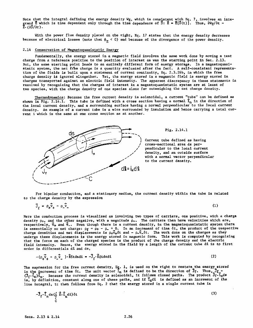
Thermodynamics: Because the free current density is solenoidal, a current "tube" can be defined as

shown in Fig. 2.14.1. This tube is defined with a cross section having a normal ýn in the direction of

the local current density, and a surrounding surface having a normal perpendicular to the local currentdensity. An example of a current tube is a wire surrounded by insulation and hence carrying a total cur-

rent i which is the same at one cross section as at another.

Fig. 2.14.1

Current tube defined as havingcross-sectional area ds per-

pendicular to the

t

density, and an outside surfacewith a normal vector perpendicularto the current density.

i

For bipolar conduction, and a stationary medium, the current density within the tube is relatedto the charge density by the expression

4.Jf = pv+ - pv_ (1)

Here the conduction process is visualized as involving two types of carriers, one positive, with a charge

density p+, and the other negative, with a magnitude p-. The carriers then have velocities which are,

respectively, v+ and _.. Even though there is a current density, in the magnetoquasistatic system there

is essentially no net charge: pf = p+ - p- = 0. In an increment of time 6t, the product of the respective

charge densities and net displacements is p+v+6t and - p.0.6t. The work done on the charges as they

undergo these displacements is the energy stored in magnetic form. This work is computed by recognizing

that the force on each of the charged species is the product of the charge density and the electric

field intensity. Hence, the energy stored in the field by a length of the current tube d£ is to first

order in differentials dt and ds,

-(pv -p_v ).E6tdsdi = -Jf*E6tdsdk (2)

The expression for the free current density, Eg. i, is used on the right to restate the energy storedin the increment of time 6t. The unit vector In is defined to be the direction of if. Thus, If =

Cf('n)tn. Because the current density is solenoidal, it follows closed paths. The product If.tndsis, by definition, constant along one of these paths, and if Indi is defined as an increment of the

line integral, it then follows from Eq. 2 that the energy stored in a single current tube is

1 d( (3)

C

Secs. 2.13 & 2.14 2.26

~

Fig. 2.14.2

Schematic representation ofa magnetoquasistatic energystorage system. Currentsare either distributed incurrent loops throughout thevolume of interest, or con-fined to one of n possiblecontours connected to thediscrete terminal pairs.

By contrast with the electroquasistatic system, in which the electric field intensity is inducedby the charge density (Gauss' law), the electric field intensity in Eq. 3 is clearly rotational. Thisemphasizes the essential role played by Faraday's law of magnetic induction.

It is helpful to have in mind at least the abstraction of a physical system. Figure 2.14.2 showsa volume of interest in which the currents are either distributed throughout the volume or confined toparticular contours (coils), the latter case having been discussed in Sec. 2.12.

First, consider the energy stored in the current paths defined by coils having cross-sectionalarea ds. From Eq. 3, this contribution to the total energy is conveniently written as

-* .nds( E.ndG)6t = Xi (4)

C.

Faraday's law and the definition of flux linkage, Eqs. 2.12.1 and 2.12.6, are the basis for representingthe line integral as a change in the flux linkage.

Because the free current density is solenoidal, the distribution of free currents within thevolume V excluded by the discrete coils can be represented as the superposition of current tubes. FromEq. 4 and the integral form of Faraday's law, Eq. 2.7.3b with vs = v = 0 (the medium is fixed), itfollows that the energy stored in a current tube is

Swcurrent tube = Jf" ndS ( A.•da) (5)

Stube

The magnetic flux density is also solenoidal4 and fog this reason it is convenient to introduce the mag-netic vector potential A, defined such that B = V x A, so that the magnetic flux density is automaticallysolenoidal. With this representation of the flux density in terms of the vector potential, Stokes'stheorem, Eq. 2.6.3, converts Eq. 5 to

Jf.*ds r 6~A.ld=r ( .6A)dsdk = J f.dAdV (6)

Ctube Ctube Vtube

Here, f is by definition in the direction of tn, so that Jf.61 takes the component of 61 in the tn direc-tion. The second equality is based upon recognition that the product as-It is a volume element of thecurrent tube, and the line integration constitutes an integration over the volume, Vtube , of the tube.

To include all of the energy stored in the distributed current loops, it is necessary only that

Sec. 2.14

Xi

2.27

the integral on the right in Eq. 6 be extended over all of the volume occupied by the tubes. The combina-tion of the incremental energy stored in the discrete loops, Eq. 4, and that from the distributed currentloops, Eq. 6, is the incremental total energy of the system

n6w = E ii i + .6AdV (7)

i=l i

In this expression, V is the volume excluded by the discrete current paths. This incremental magneticenergy storage is analogous to that for the electric field storage represented by Eq, 2.13.3.

In retrospect, it is apparent from the derivation that the division into discrete and distributedcurrent paths, represented by the two terms in Eq. 7,is a matter of convenience. In representing theincremental energy in terms of the magnetic fields alone, it is handy to extend the volume V over allof the currents within the volume of interest, including those that might be represented by discreteterminal pairs. With this understanding, the incremental change in energy, Eq. 7, is the last termonly, with V extended over the total volume. Moreover, Ampere's law represents the current density interms of the magnetic field intensity, and, in turn, the integrand can be rewritten by use of a vectoridentity (Eq. 8, Appendix B):

6w = V x H.6~dV = [H.V x A + V.(H x 6iA)]dV (8)

V V

The last term in Eq. 8 can be converted to a surface integral by using Gauss' theorem. With theunderstanding that the system is closed in the sense that the fields fall off rapidly enough at infinityso that the surface integration can be ignored, the remaining volume integration on the right in Eq. 8can be used to obtain a field representation of the incremental energy change. With the curl of thevector potential converted back to a flux density, Eq. 8 becomes

w = HfH Bdv (9)

V

The integrand of Eq. 9 is defined as an incremental magnetic energy density

6W = H.6B (10)

It is helpful to note the clear analogy between this energy density and the incremental total energyrepresented by lumped parameters. In the absence of volume free current densities that cannot berepresented by discrete terminal pairs, Eq. 7 reduces to the lumped parameter form

n6w = E i.6X. (11)

i=l

The magnetic field intensity plays the continuum role of the discrete terminal currents, and the magnetic

flux density is the continuum analog of the lumped parameter flux linkages. The situation in this mag-netic case is, of course, analogous to the electrical incremental energy storages in continuum and inlumped parameter cases, as discussed with Eqs. 7 and 8 of Sec. 2.13.

Just as it is often convenient in dealing with electrical lumped parameters to use the voltageas an independent variable, so also in magnetic field systems it is helpful to use the terminal currentsas independent variables. In that case, the coenergy function w' is conveniently introduced as anenergy function

n6w' = Z X.6i. (12)

1 1i=l

In an analogous way, the co-energy density, w', is defined such that

6W' = B.6H; W' = H.B - W (13)

Power Flow: Thus far, the storage of energy in magnetic form has been examined. The postulatehas been that all work done in moving the charges against an electric field is stored. In any systemas a whole this is not likely to be the case. The general magnetoquasistatic laws enable a deductionof an equation representing the flow of power, and the rate of change of the stored energy. This places

Sdc. 2.14 2.28

the energy storage in the context of a more general system.

A clue as to how an energy conservation statement might be constructed from the differential mag-netoquasistatic laws is obtained from Eq. 2, which makes it clear that the product of the free currentdensity and the electric field intensity are closely connected with the statement of conservation ofenergy. The dot product of the electric field and Ampere's law, Eq. 2.3.23b, is

E.[V x H - Jf] - 0 (14)

Use of a vector identity 6Eq. 8, Appendix B) makes it possible to rewrite this expression as

+ 4. 4. 4. 4. 4.H.V x E - V.(E x H) = E.Jf (15)

With the additional use of Faraday's law to represent V x E, Eq. 15 takes the form of Eq. 2.13.16, with

S EExHe

1 4.We - H (16)

4+.+ 4. o +-E.J - H. - x (. Mx )

These quantities have much the same physical significances discussed in connection with Eq. 2.13.16.

To place the magnetic energy storage identified with the thermodynamic arguments in the context ofan actual system, consider a material which is ohmic and fixed so that 4 = 0 and If = C1. Then thesecond term on the right in Eq. 16c is in the form of a time rate of change of magnetization energydensity. Hence, the power flow equation assumes the form of Eq. 2.13.17, with

WE= H*6B (17)o

SE = -QE*E

Implicit is the assumption that H is a single-valued function of the instantaneous B. The resultingenergy density includes magnetization energy and is consistent with Eq. 2.14.10.

2.15 Complex Amplitudes; Fourier.Amplitudes and Fourier Transforms

The notion of a continuum network fs introduced for the first time in the next section. The associ-ated transfer relations illustrated there are a theme throughout the chapters which follow. Among severalreasons for their use is the organization they lend to the representation of complicated, largely linear,systems. In this chapter, the continuum networks represent electromagnetic fields. Later, they re-present fluid and (to some degree) solid mechanics, heat and mass transfer, and electromechanical continuain general. These networks make it possible to set aside one part of a given problem, derive the associ-ated relations once and for all and accumulate these for later use. Such relations will be picked up overand over in solving different problems and, properly understood, are a useful reference.

Complex Amplitudes: In many practical situations, excitations are periodic in one or two spatialdirections, in time or in space and time. The complex amplitude representation of fields, useful indealing with these situations, is illustrated by considering the function O(z,t) which has dependenceon z given explicitly by

O(z,t) = Re ý ( t ) e - j k z (1)

With the wavenumber k real, the spatial distribution is periodic with wavelength X = 2wr/k and spatialphase determined by the complex amplitude 1. For example, if ý= o(t) is real and k is real, thenO(z,t) = o00 (t) cos kz.

The spatial derivative of 0 follows from Eq. 1 as

S Re (t)e-jkz (2)7z Re.[-JkZ(t)e (2

Secs. 2.14 & 2.152.29

The following identifications can therefore be made:

as

with it being understood that even though complex amplitudes are being used, the temporal dependence isarbitrary. There will be occasions where the time dependence is specified, but the space dependence isnot. For example, complex amplitudes will take the form

Q(z,t) = Re4(z)e j wt (4)

where D(z) is itself perhaps expressed as a Fourier series or transform (see Sec. 5.16).

Most.often, complex amplitudes will be used to represent both temporal gnd spatial dependences:

D(z,t) = Recej(Wt-kz) (5)

The (angular) frequency w can in general be complex. If 0 is periodic in time with period T, then T =2n/w. For complex amplitudes 0, the identifications are:

[4(z,t), (z,t), (z,t)]<>[$,-jk(,jj] (6)

If w and k are real, Eq. 5 represents a traveling wave. At any instant, its wavelength is 2w/k,at any position its frequency is w and points of constant phase propagate in the +z direction with thephase velocity w/k.

Fourier Amplitudes and Transforms: The relations between complex amplitudes are identical to thosebetween Fourier amplitudes or between Fourier transforms provided that these are suitably defined. Fora wide range of physical situations it is the spatially periodic response or the temporal sinusoidalsteady state that is of interest. Simple combinations of solutions represented by the complex amplitudesthen suffice, and there is no need to introduce Fourier concepts. Even so, it is important to recognizeat the outset that the spatial information required for analysis of excitations with arbitrary spatialdistributions is inherent to the transfer relations based on single-complex-amplitude solutions.

The Fourier series represents an arbitrary function periodic in z with fundameqtal periodicitylength k by a superposition of complex exponentials. In terms of complex Fourier coefficients $n(t),such a series is

-jkn z

Q(z,t) = E (t)e k 2nI/R; Q* = n (7)n n n -n

where the condition on 4n insures that 0 is real. Thus, with the identification n+ 4n and k + kn, eachcomplex exponential solution of the form of Eq. 1 can be taken as one term in the Fourier series. Themth Fourier amplitude Om follows by multiplying Eq. 7 by the complex conjugate function exp(jkmz) and.integrating over the length k to obtain only one term on the right. This expression can then be solved

for ým to obtain the inverse relation

1 z+ Jkmzim OQ(z,t)e dz (8)

z

If the temporal dependence is also periodic, with fundamental period T, the Fourier series can also

be used to represent the time dependence in Eq. 7:

+i +o J wmt-knz)

O(z,t)= E E 5 e ; * = 8 (9)mn mn -m-nm=-- n=-•

where the condition on the amplitudes insures that O(z,t) is real. One component out of this double sum-mation is the traveling-wave solution represented by the complex amplitude form, Eq. 5. The rules givenby Eqs. 3 and 6 pertain either to the complex amplitudes or the Fourier coefficients.

The Fourier transform is convenient if the dependence is not periodic. With the Fourier transform

0(k,t) given by

0(k,t) = + S(z,t)ejkZ dz

Sec.215 2.3

Sec. 2.15 2.30

the functional dependence on z is a superposition of the complex exponentials

+ooO(zt) f 0i(k,t)e- kz dk

-00

The relation between the transform and the transform of the derivative can be found by taking the trans-form of 30/3z using Eq. 11 and integrating by parts. Recall that fvdu = uv - fudv and identifydu -+ O/azdz and v - exp jkz, and it follows that

S- kz dz = ejk-C -jk + ejkz dz (12)

For properly bounded functions the first term on the right vanishes and the second is -jki(k,t). Thetransform of Ha/Dz is simply -jkl and thus the Fourier transform also follows the rules given withEq. 3.

Extension of the Fourier transform to a second dimension results in the transform pair

j(ot-ks) dk dw0(z,t) = 0 $(k, w)eJ(t-kz) 2dkd2w

(13)

A +| -j (,t-kz) dt dzJ(k,w)= f (z,t)e - j (tkz)dt dz

which illustrates how the traveling-wave solution of Eq. 5 can be viewed as a component of a complicatedfunction. Again, relations between complex amplitudes are governed by the same rules, Eq. 6, as are theFourier amplitudes $(k,w).

If relationships are found among quantities $(t), then the same relations hold with c + $ andD( )/Bt -÷ jw, because the time dependence exp(jwt)is a particular case of the more general form $(t).

Averages of Periodic Functions: An identity often used to evaluate temporal or spatial averages ofcomplex-amplitude expressions is

Re ekz Re Bej = 1 Re A B* (14)/z 2

where ( )zsignifies an average over the length 2w/k and it is assumed that k is real. This relationfollows by letting

Re A ejkz Re e-jkz = ejkz + A*ejk]2 e-jkz + eejk] (15)

and multiplying out the right-hand side to obtain

'IBe-2jkz + X*i*e2jk + B*+ A* (16)

The first term is a linear combination of cos 2kz and sin 2kz and hen e averages to zero. The secondterm is constant and identical to the right-hand side of Eq. 14.

A similar theorem simplifies evaluation of the average of two pe odic functions expressed in theform of Eq. 7:

-jknz +- -jkmZA /_1 r= -

= AB = AB*n -n n nSn=--0 mo

(17)

Sec. 2.152.31

Of course, either the complex amplitude theorem of Eq. 14 or the Fourier amplitude theorem of Eq. 17applies to time averages with kz - -wt.

2.16 Flux-Potential Transfer Relations for Laplacian Fields

It is often convenient in the modeling of a physical system to divide the volume of interest intoregions having uniform properties. Surfaces enclosing these regions are often planar, cylindrical orspherical, with the volume then taking the form of a planar layer, a cylindrical annulus or a sphericalshell. Such volumes and bounding surfaces are illustrated in Tables 2.16.1-3. The question answeredin this section is: given the potential on the bounding surfaces, what are the associated normal flux

densities? Of immediate interest is the relation of the electric potentials to the normal displace-ment vectors. But also treated in this section is the relation of the magnetic potential to the normalmagnetic flux densities. First the electroquasistatic fields are considered, and then the magnetoquasi-static relations follow by analogy.

Electric Fields: If any one of the regions shown in Tables 2.16.1-3 is filled with insulatingcharge-free (pf O) material of uniform permittivity e,

S(- )E, D = E (1)

the governing field equations are Gauss' law, Eq. 2.3.23a,

V*D = 0 (2)

and the condition that E be irrotational, Eq. 2.3.24a. The latter is equivalent to

E = -V0 (3)

Thus, the potential distribution within a volume is described by Laplace's equation

V20 = 0 (4)

In terms of 4,

D = -eVO (5)

Magnetic Fields: For magnetoquasistatic fields in an insulating region (Jf = 0) of uniform per-meability

M= (I-- 1)Hi;.B =pH (6)110

Thus, from Ampere's law, Eq. 2.3.23b, H is irrotational and it is appropriate to define a magnetic

potential Y:

H = -V_ (7)

In addition. there is Eq. 2.3.24b:

V.B = 0 (8)

Thus, the potential again satisfies Laplace's equation

v2y = 0 (9)

and in terms of ', the magnetic flux density is

B = -1VW (10)

Comparison of the last two relations to Eqs. 4 and 5 shows that relations now derived for theelectric fields can be carried over to describe the magnetic fields by making the identification

Planar Layer: Bounding surfaces at x = A and x = 0, respectively denoted by a and 0, are shown

in Table 2.16.1. So far as developments in this section are concerned, these are not physical boundaries

They are simply surfaces at which the potentials are respectively

4(A,y,z,t) = Reg (t)exp[-j(ky+kz)]; D(0,y,z,t) = Re I 0(t)exp[-j(ky+kzz)] (11)y( zy yt

Secs. 2.15 & 2.16 2.32

Table 2.16.1. Flux-potential -transfer relations for planar layer in terms of electricpotential and normal displacement (0,Dx). To obtain magnetic relations,substitute (Q,Dx,) +e ('Y,.B,).

These will be recognized as generalizations of the complex amplitudes introduced with Eq. 2.15.1. Thatthe potentials at the a and $ surfaces can be quite general follows from the discussion of Sec. 2.15,which shows that the following arguments apply when I is a spatial Fourier amplitude or a Fourier trans-form.

In view of the surface potential distributions, solutions to Eq. 4 are assumed to take the form

S=-Re O(x,t) exp[-j(kyy + kzz)] (12)

Substitution shows that

d2 2 = 0; y =Vk2 + k2 (13)

dx2 y z

+yxSolutions of this equation are linear combinations of e or alternatively of sinh yx and cosh yx.With ~i and 12 arbitrary functions of time, the solution teakes the form

0$1 sinh yx + 02 cosh yx (14)

The two coefficients are determined by requiring that the conditions of Eq. 11 be satisfied. For the sim-ple situation at hand, an instructive alternative to performing the algebra necessary to evaluate (01,02)consists in recognizing that a linear combination of the two solutions in Eq. 14 is sinh y(x - A). Thus,the solution can be written as the sum of solutions that are individually zero on one or the other of thebounding surfaces. By inspection, it follows that

a- sinh.yx _ .; sinh y(x - A) (15)sinh yA sinh yA

From Eqs. 5 and 15, 1can be determined:

-e Re a cosh yx -B cosh y(x-A) - (ky + kz) (16)x ax Ry sinh yA sinh yA

Evaluation of this equation at x - A gives the displacement vector normal to the a surface, with complexamplitude ED. Similarly, evaluated at x = 0, Eq. 16 ives D5. The components of the "flux" (Nij ) are

now determined, given the respective potentials (ci ,B). The transfer relations, Eq. (a) of Table 2.16.1,

summarize what is found. These relations can be solved for any pair of variables as a function of theremaining pair. The inverse transfer relations are also summarized for reference in Table 2.16.1, Eq. (b)

Sec. 2.16

I

2.33

Ix

YA-(a) (b)

Fig. 2.16.1. (a) Transfer coefficients as a function of Ay EA k2 + k2(b) Distribution of 0 across layer.

That the layer is essentially a distributed capacitance (inductance) is emphasized by drawingattention to the analogy between the transfer relations and constitutive laws for a system of linearcapacitors (inductors). For a two-terminal-pair system, Eq. 2.11.5 comprises two terminal char es

(ql,q2) expressed as linear functions of the terminal voltages (vl,V2). Analogously, the (D,,Dx)(which have units of charge per unit area and an arbitrary time dependence) are given as linear func-tions of the potentials by Eq. (a) of Table 2.16.1. A similar analogy exists between Eq. 2.12.5,expressing (X1 ,X2 ) as functions of (il,i 2), and the transfer relations between (B ,BO) (units of fluxper unit area) and the magnetic potentials (TYa,P).

According to Eq. (a) of Table 2.16.1, Dx is induced by a "self term" (proportional to the potentialat the same surface) and a "mutual term." The coefficients which express this self- and mutual-couplinghave a dependence on ay (2r/y the wavelength in the y-z plane) shown in Fig. 2.16.1a. Written in theform of Eq. 15, the potential has components, excited at each surface, that decay to zero, as shown inFig. 2.16.1b, at a rate that is proportional to how rapidly the fields vary in the y-z plane. For longwaves the decay is relatively slow, as depicted by the case Ay = 0.5, and the mutual-field is almost asgreat as the self field. But as the wavelength is shortened relative to A (Ay increased), the surfacescouple less and less.

In this discussion it is assumed that y is real, which it is if ky and kz are real. In fact, thetransfer relations are valid and useful for complex values of (ky,kz). If these numbers are purelyimaginary, the field distributions over the layer cross section are periodic. Such solutions are neededto satisfy boundary conditions imposed in an x-y plane.

Cylindrical Annulus: With the bounding surfaces coaxial cylinders having radii a and B, it isnatural to use cylindrical coordinates (r, 0, z). A cross section of this prototype region and thecoordinates are shown in Table 2.16.2. On the outer and inner surfaces, the potential has the respective forms

o(a,e,z,t) = Re P (t) e- j(me+kz); 0(B,0,z,t) = Re ~ (t)e-j(me+kz) (17)

Hence, it is appropriate to assume a bulk potential

( = Re ý(r,t)e -j(me+kz) (18)

Substitution in Laplace's equation (see Appendix A for operations in cylindrical coordinates), Eq. 4,then shows that

d 1 d@ 2 m (19)+ - - (k +•) 0 (19)

dr2 r dr 2dr r

By contrast with Eq. 13, this one has space-varying coefficients. It is convenient to categorize thesolutions according to the values of (m,k). With m = 0 and k = 0, the remaining terms are a perfectdifferential which can be integrated twice to give the solutions familiar from the problem of the field

Sec. 2.16 2.34

)"A=.5 V YA= 2 &8 YA=5 V

Table 2.16.2. Flux-potential relations for cylindrical annulus in terms of electric potential andnormal displacement (0,Dr). To obtain magnetic relations, substitute (0,Dr,E)+(T,Br,).

0 = Re 0(r,t)e- j (mO + kz)

fm(B~a)

CI~B ll fm (a, 8) 8 ,

k = 0 = 0

fo(x,y) = n) g (x,y) = n(?)

k = 0, mi 1,2,...

f (x,)

x1gm(x,y) = 2 m

x E(- - ()

k 0, m = 0i1,2n..*

jk[H (jkx)J'(jky) - Jm(jkx)Hm(jky)]

fm(x,y) - EJm(jkx)Hm(jky) - Jm(jky)Hm(jkx)]

gm.(x,y) = rx[Jm(jkx)H (jky) - Jm(jky) Im(Jkx)]

fm(X,y) =

gm(x,y) =

k[Km(kx)Im(ky) - Im(kx)K'(ky) ]

[Im(kx)Km(ky) - Im(ky)Km(kx)]

1) - IX[Im(kx)Km(kY) - Im(ky)Km(kx)]

G (a,) Bam r

F (at,) BOI~L rJL JI6

k = 0, m = 0

No inverse

k = 0, m = 1,2,***x m

n in[( )im (Z ]

G (x,y) = 1m (x)m a

y x

k 0 0 m = 0,1,2,.in*

1 [J(jkx)Hm(jky) - Hm(jkx)Jm(jky)]

F(x,y) =T-[Jm(jky)H'(jkx) - Jm(jkx)Hm (jky)]

-2Gm(xy) = jk(kx) [J(jky)H'(Jkx)-Jm(Jkx)Hm(ky)

Fm(x,y) =

G3 (x,y) =

1 [.(kx)Km (ky) - Km(kx)Im(ky)]k [Im(ky)Km(kx) - Im(kx)Km(ky) ]

k(kx) [I'(kv)K'(kx) - I'(kx)K'(kv)]- nmm-- - mi m

kI' (ka)0 0 r = f (,O) 4 ; fC(0 ) =(- in(k) (c)

Sr m m Im(k)

See Prob. 2.17.2 for proof that Hm(jkx)Jl(jkx) - Jm(jkx)H'm(jkx) = -2/(rkx) and Km(kx)I(kx)- Im(kx)K(kx) = 1/kx incorporated into gm and GM.

r__

2.35 Sec. 2.16

0 I 2 3

ka or k--(b)

Fig. 2.16.2. (a) Modified Bessel functions. (b) Self-field coefficients of cylindricaltransfer relations in limits where surfaces do not interact.

between coaxial circular conductors. In view of the boundary conditions at r = a and r = 8,

In (-)

In •) a+ (B - i )8 a

In (-)

In (&)a

(m,k) = (0,0)

For situations that depend on 6, but not on z (polar coordinates) so that k = 0, substitution shows thesolutions to .Eq.19 are r- . By inspection or algebraic manipulation, the linear combination of thesethat satisfies the conditions of Eq. 17 is

I[(m-( (i)r]i,c r,

a a8-[)m_)] (m,k) -= (,O)a -

For k finite, the solutions to Eq. 19 are the modified Bessel functions Im(kr) and Km(kr). These playa role in the circular geometry analogous to exp(+yx)in Cartesian geometry. The radial dependences ofthe functions of order m = 0 and m = 1 are shown in Fig. 2.16.2a. Note that Im and Km are respectivelysingular at infinity and the origin.

Just as the exponential solutions could be determined from Eq. 13 by assuming a power series in x,the Bessel functions are determined from an infinite series solution to Eq. 19. Like y, k can in generalbe complex. If it is, it is customary to define two new functions which, in the special case where kis real, have imaginary arguments:

(22)Jm(Jkr) j mI (kr), H (jkr) j-(m Kl)(kr)m m m 7r m

These are respectively the Bessel and Hankel functions of first kind. For real arguments, Im and Km arereal, and hence Jm and Hm can be either purely real or imaginary, depending on the order.

Large real-argument limits of the functions Im and Km reinforce the analogy to the Cartesian

"ec. 2.16

U

(a)

in (a)(20)

(21)

2.36

exponential solutions:

lim Im(u) = exp (u) ;lim Km(u) = exp(-u) (23)U-n-o V2S U-wo

Useful relations in the opposite extreme of small arguments are

lim jH (ju) = 2 In (; lim Jm(ju) =u 0 T 1.781072u m m2 m

(24)

lim H (ju) =(m - 1 ) 2m ; m 0u+0 m jr(ju) m

By inspection or algebraic manipulation, the linear combination of J and H satisfying the boundaryconditions of Eq. 17 is m m

[H (jkB)Jm(jkr) - Jm(JkB)H (jkr)] [Jm(jka)H kr)r) - H (jka)Jm(jkr)]=v mm + m -m mm m (25)

[Hm(jkB)Jm(jka) - Jm(jk)H (jka)] [Jm(jka)Hm (jk) - Hm(jka) m(Jk)] (25)

The evaluation of the surface displacements (Da,Dr) using Eqs. 20, 21, or 25 is now accomplishedusing the same steps as for the planar layer. The resulting transfer relations are summarized byEq. (a) in Table 2.16.2. Inversion of these relations, to give the surface potentials as functions ofthe surface displacements, results in the relations summarized by Eq. (b) of that table. Primes denotederivatives with respect to the entire specified argument of the function. Useful identities are:

uI'(u) = m (u) + uIm+l(u); UI'(u) = -mI (uy + uI (u)

uK'(u) = mK (u) - uK (u)m m m+l

R'(u) = -R1 (U) (26)

uR'(u) = -mR (u) + uRm_(u); uR'(u) = mR (u) - uR (u)m m m-1 m m m+1

where Rm can be Jm, H , or the function N to be defined with Eq. 29.

Two useful limits of the transfer relations are given by Eqs. (c) and (d) of Table 2.16.2. Inthe first, the inner surface is absent, while in the second the outer surface is removed many wave-lengths 2w/k. The self-field coefficients fm(O,a) and fm(o,8) are sketched for m=0O and m=l inFig. 2.16.2b. Again, it is useful to note the analogy to the planar layer case where the appropriatelimit is kA - m-. In fact, for ka or kB reasonably large, the k dependence and the signs are thesame as for the planar geometry:

lim fm(0O,a) -+ -ka; lim Bf(oO,B)U ký (27)ka-m kB+

For small arguments, these functions become

lim af (0,a) _ -_(k) 2 ; lim Bf (0 ,0) - 1kao0 o 2 kB+0 ln [1.781072kB

(28)

lim afm(O,a) - -m for m 0 0; lim 8fm(CO8) + m for m # 0ka-0O kB+0

In general, k can be complex. In fact the most familiar form for Bessel functions is with k purelyimaginary. In that case, Jm is real but Hm is complex. By convention

H (u) E Jm(U) + JNm(u) (29)

where, if u is real, Jm and Nm are real and Bessel functions of first and second kind. As might be

expected from the planar analogue, the radial dependence becomes periodic if k is imaginary. Plots

of the functions in this case are given in Fig. 2.16.3.

Sec. 2.162.37

Fig. 2.16.3. Bessel functions of first and second kind and real arguments. Referencesfor the Bessel and related functions should be consulted for more detailsconcerning their properties and numerical values. 1-4

Spherical Shell: A region between spherical surfaces having outer and inner radii a and 8, respectively, is shown in the figure of Table 2.16.3. In the volume, the potential conveniently takes thevariable separable form

4 = Re i(r,t) e(e)e - jmO (30)

where (r,68,) are spherical coordinates as defined in the figure. Substitution of Eq. 30 into Laplace'sequation, Eq. 4, shows that the 0 dependence is correctly assumed and that the (r,8) dependence isdetermined from the equations

1 d [sin d m _K2

sin 80 d d sin2sin e(31)

1 d ,_2 d _ 2-dr dr

where the separation coefficient K2 is independent of (r,e). With the substitutions

u = cosO, V-u = sin 6 (32)

Eq. 31a is converted to

2 2(1 - u2 ) 2u + (K2 _ -- 2) 0 = 0 (33)duu -u2

du 1-u

For K2 = n(n+l) and n an integer, solutions to Eq. 33 are

0 = Pm(u) (34)n

1. F. B. Hildebrand, Advanced Calculus for Applications, Prentice-Hall, Englewood Cliffs, N.J., 1962,pp. 142-165.

2. S. Ramo, J. R. Whinnery and T. Van Duzer, Fields and Waves in Communication Electronics, John Wileyand Sons, New York, 1965, pp. 207-218.

3. M. Abramowitz and I. A. Stegun, Handbook of Mathematical Functions with Formulas, Graphs, and Mathe,matical Tables, National Bureau of Standards, Applied Mathematics Series 55, U.S. Government PrintiiOffice, Washington D. C. 20402, 1964, pp. 355-494.

4. E. Jahnke and F. Emde, Table of Functions with Formulae and Curves, Dover Publications, New York.1945, pp. 128-210.

m

Table 2.16.3. Flux-potential transfer relations for spherical shell in terms of electric

potential and normal displacement (0,Dr). To obtain magnetic relations,

substitute (0,Dr,E) + (',Br,1).

Sec. 2.162.39

where Pm are the associated Legendre functions of the first kind, order n and degree m. In terms of theLegendre polynomials Pn, these functions are summarized in Table 2.16.3. Note that these solutions areclosed. They do not require infinite series for their representation.

To the second order differential equation, Eq. 33, there must be a second set of solutions Q.Because these are singular in the interval 0 4 e < 7 , and situations of interest here include theentire spherical surface at any given radius, these solutions are not included. The functions Pm playthe role of exp(jkz)(say) in cylindrical geometry, while exp(jmo) is analogous to exp(jmO). The radialdependence, which is much of the bother in cylindrical coordinates, is actually quite simple in sphericalcoordinates. From Eq. 31b it is seen that solutions are a linear combination of rn and r-(n+l). Withthe assumption that surface potentials respectively have the form

t(a,e,0,t) = Re $ (t)P m (cose) exp(jmo) (35)

it follows that the appropriate linear combination is

[(r)n _ n+l rn n+l; r '+ r (36)

[()n _ n+l n a n+(36)

The complex amplitudes (P,PB) determine the combination of cos mo and sin mý, constituting the dis-tribution of Q with longitudinal distance. For a real amplitude, the distribution is proportional tocos mý. In the summary of Table 2.16.3, the lowest orders of Pg (cos 0) are tabulated, together withdiagrams showing the zones that are positive and negative relative to each other. In the rectangularplots, the ordinate is 0( 0 4 7, while the abscissa is 0 < 0 < 27. Thus, the top and bottom lines arethe north and south poles while the lines within are nodes. The horizontal register of each diagram isdetermined by the complex amplitude, which determines the phase of exp(jmo).

Evaluation of the transfer relations given in Table 2.16.3 by Eqs. (a) and (b) is now carried outfollowing the same procedure as for the planar layer. From these relations follow the limiting situ-ations of a solid spherical region or one where the outer surface is well removed from the region ofinterest summarized for reference by Eqs. (c) and (d) of Table 2.16.3.

Further useful aspects of solutions to Laplace's equation in spherical coordinates, includingorthogonality relations that permit Fourier-like expansions and evaluation of averages, are given instandard references.5

2.17 Energy Conservation and quasistatic Transfer Relations

Applied to one of the three regions considered in Sec. 2.16, the incremental total electric energygiven by Eq. 2.13.6, can be written as

w = - V6DdV = - fV.(6)dV + fV*6DdV (1)

V V V

Because pf = 0, the last integral is zero. The remaining integral is converted to a surface integral byGauss' theorem, and the equation reduces to

dw = - 066.nda (2)

S

Similar arguments apply in the magnetic cases. Because there is no volume free current density,H = -VT and Eq. 2.14.9 becomes

6w = - d'B'nda (3)

SConsider now the implications of these last two expressions for the transfer relations derived in

Sec. 2.16. Discussion is in terms of the electrical relations, but the analogy made in Sec. 2.16 clearl1pertains as well to Eqs. 2 and 3, so that the arguments also apply to the magnetic transfer relations.

Suppose that the increment of energy 6w is introduced through S to a volume bounded by sections of

the a and B surfaces extending one "wavelength" in the surface dimensions. In Cartesian coordinates,

5. F. B. Hildebrand, loc. cit., pp. 159-165.

Secs. 2.16 & 2.17 2.40

this volume is bounded by (y,z) surfaces extending one wavelength in the y and z directions. In cylin-drical coordinates, the volume is a pie-shaped cylinder subtended by outside and inside surfaces havinglength 2w/k in the z direction and 2wa/m and 2rB/m respectively in the azimuthal direction. In sphericalcoordinates, the volume is a sector from a sphere with 0 = 2w/m radians along the equator, 6 extendingfrom 0 + w and the surfaces at r = a and r = 8. In any of these cases, conservation of energy, asexpressed by Eq. 2, requires that

6w = -aaKKa6D + a 0B6D8 (4)

The ( )> indicate averages over the respective surfaces of excitation. The areas (a ,a ) are inparticular

ar (2 22/kyk Cartesian

as [(27) 2 /mk](') cylindrical (5)

(4w/m) a2 spherical

In writing Eq. 2 as Eq. 4, contributions of surfaces other than the a and $ surfaces cancel becauseof the spatial periodicity. It is assumed that (ky,kz), (m,k) and m are real numbers.

The transfer relations developed in Sec. 2.16 take the general form

a -All A2 D= (6)

The coefficients Ai- are real. Hence, for the purpose of deducing properties of Aij, there is no loss

in generality in ttiing (Dni,D)and hence (~a•) as being real. Then, Eq. 4 takes the form

6w = C[-aa &o + a•n nD)- (7) /n n

where C is 1/2 in the Cartesian and cylindrical cases and is a positive constant in the spherical

case.

With the assumption that w = w(Da,D ), the incremental energy can also be written as

6w = a6wa +w B (8)aDa n S nn n

where (Mn,aB) constitute independent electrical "terminal" variables. Thus, from Eqs. 7 and 8,n n

_alra= awaS = w_ (9)

n n

A reciprocity condition is obtained by taking derivatives of these expressions with respect to B0 and&, respectively, and eliminating the energy function. In view of the transfer relations, Eq. 6,n

aaAl2 = a0A21 (10)

Thus, in the planar layer where the areas a" and a are equal, the mutual coupling terms A12 = A21.That the relations are related by Eq. 10 in the spherical case is easily checked, but the complicatedexpressions for the cylindrical case simplify the mutual terms (footnote to Table 2.16.2).

The energy can be evaluated by in egrating Eq. 7 using the "constitutive" laws of Eq. 6. Theintegration is first carried out with D f 0, raising ia to its final value. Then, with Da - ba, OBisraised to its final value

w = C a Alla () 2 - a A21n•ab + 1 a A22 (0) (11)

Sec. 2.172.41

With either excitation alone, w must be positive and so from this relation it follows that

A11 > 0, A22 > 0 (12)

These conditions are also met by the relations found in Sec. 2.16.

2.18 Solenoidal Fields, Vector Potential and Stream Function

Irrotational fields, such as the quasistatic electric field, are naturally represented by a scalarpotential. Not only does this reduce the vector field to a scalar field, but the potential functionevaluated on such surfaces as those of "perfectly" conducting electrodes becomes a lumped parameterterminal variable, e.g., the voltage.

Solenoidal fields, such as the magnetic flux density B, are for similar reasons sometimes re-presented in terms of a vector potential A:

+ +Thus, B automatically has no divergence. Unfortunately, the vector field B is represented in terms ofanother vectox field A. However, for important two-dimensional or symmetric configurations, a singlecomponent of A is all required to again reduce the description to one involving a scalar function.Four commonly encountered cases are summarized in-Table 2.18.1.

The first two are two-dimensional in the usual sense. The field B lies in the x-y (or r-8) planeand depends only on these coordinates. The associated vector potential has only a z component. Thethird configuration, l1ke the second, is in cylindrical geometry, but with B independent of e and hencewith A having only an i0 component. The fourth configuration is in spherical geometry with symmetryabout the z axis and the vector potential directed along 0..

Like the scalar potential used to represent irrotational fields, the vector potential is closelyrelated to lumped parameter variables. If B is the magnetic flux density, i4 is convenient for evalua-tion of tje flux linkage X (Eq. 2.12.1). For an incompressible flow, where B is replaced by the fluidvelocity v, the vector potential is conveniently used to evaluate the volume rate of flow. In thatapplication, A and A become "stream functions."

The connection between the flux linked and the vector potential follows from Stokes's theorem,Eq. 2.6.3. The flux 1X through a surface S enclosed by a contour C is

0= f 1da =a V x -tnda= 1d- (2)

S S C

In each of the configurations of Table 2.18.1, Eq. 2 amounts to an evaluation of the surface integral.For example, in the Cartesian two-dimensional configuration, contributions to the integration around acontour C enclosing a surface having length 2 in the z direction, only come from the legs running inthe a direction. Along these portions of the contour, denoted by (a) and (b), the coordinates (x,y) are

constant. Hence, the flux through the surface is simply 2 times the difference A(a) - A(b), as sum-marized in Table 2.18.1.

In the axisymmetric cylindrical and spherical configurations, r and r sin 6 dependences arerespectively introduced, so that evaluation of A essentially gives the flux linked. For example, inthe spherical configuration, the flux linked by a surface having inner and outer radii r cos 0 evaluatedat (a) and (b) is simply

SA(,rsin e .d= r sin e 2(r sin e)b = 2rI[A(a) - A(b)] (3)

C

Used in fluid mechanics to represent incompressible fluid flow, A is the Stokel's stream function. Notethat the flux is positive if directed through the surface in the direction of n, which is specified interms of the contour C by the right-hand rule.

2.19 Vector Potential Transfer Relations for Certain Laplacian Fields

Even in dealing with magnetic fields in regions where Jf = 0,if the flux linkages are of interest,it is often more convenient to develop a model in terms of transfer relations specified in terms of avector rather than scalar potential. The objective in this section is to summarize these relations forthe first three configurations identified in Table 2.18.1.

Secs. 2.17, 2.18 & 2.19 2.42

Table 2.18.1.

Important configurations having solenoidal field B represented by single components of vector potential A.

Two-dimensional Cartesian

ttA

= A(x,y)iz

(a)

@ BA -

A

BA

B

=

-i

i

(b)

4y

x ax

y

== £[

A(a

) -

A(b

)]

(c)

Polar

Axisymmetric cylindrical

A=

A(r,O)iz

(d)

A

= rz

(g)

+ 1 aA+

A

+

1 A

1

AABa

i

A i

e (e

) B

-r

rra-

r -r

rra

z r

r r

z h

S=

£[

A(a)

-A(b)]

(f)

I =

2r[

A(a

) -

A(b

)]

(i)

Axisymmetric spherical

r si

n 80

(j)

B

1 1

lA

A

(-

r si

n [

r

D8

r ie

(k

)

4ý

=27

[A(a

) -

A(b

)]

(1)

Table 2.19.1.

Vector potential transfer relations for two-dimensional or symmetric Laplacian fields.

Two-dimensional Cartesian

Polar

Axisymmetric cylindrical

-o

.-.a

I/

A

Hz

I fZ

z

A

= i z

Re

A(x

) exp(-jky)

A=

iz

Re

A(r

) exp(-jmA)

A=

i, R

e A

(r)e

xp(-

jkz);

A

= Ar

Sr1

-(e1

-cot

h(kA

A)

fsinh(k)

1

m(

) gm

(a,

c ) k2

F

(~c)

Go(

c,~

k(a)

(c)

(e)

=

[

1 coth(kA)

A

(B,a

) f m

(a,)

G

H

G(~

) F

(a

,)y

Lsin

h(k

A)

m

z

-co

th(k

A)

sin

h(k

A)

Hy

F (,

a)

GM6a

,1)

( fo

(,i)

1 [(

a,

) H

zS

sh

si

nh(k

A)

y

m•(

I,)

o((,

)

I1S(b)

= p

(d)

= -()

(f)

k -1

(kA )L

1LL

sinh

(kA)

JL

Y

L J

M

m

J3

0

z

For fm, gm, Fm, Gm see Table 2.16.2,

For Fo, G , fo

go see Table 2.16.2,

k =

0,

m

# 0

m =

0,

k 0

IIx

1 r

a r

LB kB

A

m B

[[J

kJ[J

I I

4 +With B represented in terms of A by Eq. 2.18.1, Ampere's law (Eq. 2.3.23) requires that in a region

of uniform permeability p,

V x V x A = 1Jf (1)

S+ +For a given magnetic flux density B, cull A is specified. But to make A unique, its divergence _ust alsobe specified. Here, the divergence of A is defined as zero. Thus, the vector identity V x V x A =V(V.A) - V21 reduces Eq. 1 to the vector Poisson's equation:

V = -1Jf; VAi =0 (2)

The vector Laplacian is summarized in Appendix A for the three coordinate systems of Table 2.18.1. Eventhough the region described in the following developments is one where Jf = 0, the source term on theright has been carried along for later reference.

Cartesian Coordinates: In the Cartesian coordinate system of Table 2.18.1 it is the z componentof Eq. 2 that is of interest. The z component of the vector Laplacian is the same operator as for thescalar Laplacian. Thus, the situation is analogous to that outlined by Eqs. 2.16.11 to 2.16.16 with0 - A. With solutions of the form A = Re A(x,t) exp(-jky) so that y + k E k, the appropriate linearcombination of solutions is Y

~o sinh kx - sinh k(x - 4)sinh kA sinh kA (3)

Because H = B/p, the associated tangential field intensity is given by Eq. (b), Table 2.18.1,

1 aAHy I @(4)y 1I ax

Expressed in terms of Eq. 3 and evaluated at the surfaces x = a and x = 8, respectively, Eq. 4 givesthe first transfer relations, Eq. (a), of Table 2.19.1. Inversion of these relations gives Eqs. (b).

Polar Coordinates: In cylindrical coordinates with no z dependence, it is again the z componentof Eq. 2 that is pertinent. The configuration is summarized in Table 2.18.1. Solutions take theform A = Re A(r,t) exp(-jme) and are analogous to Eq. 2.16.21 with 0 replaced by A:

4m rrm r m a m

r 0 + a (5)[( m am m ()m

The tangential field is then evaluated from Eq. (e), Table 2.18.1:

1 aAHe 9ar (6)

Evaluation at the respective surfaces r = a and r = 8 gives the transfer relations, Eqs. (c) ofTable 2.19.1. Inversion of these relations gives Eqs. (d).

Axisymmetric Cylindrical Coordinates: By contrast with the two-dimensional configurations so farconsidered, where the vector Laplacian of Az is the same as the scalar Laplacian, the vector nature ofEq. 2 becomes apparent in the axisymmetric cylindrical configuration. The 0 component of Eq. 2 is thescalar Laplacian of A0 plus (-AI/r2 ) (see Appendix A). With A0 E A,

2a 1 LA A a2A2 r ar r 2 (2 7)

Even though solutions do not have a 6 dependence, so that

A = Re A(r,t)e-jkz (8)

equation 7 reduces to a form of Bessel's equation to which solutions are Bessel's and Hankel's func-tions of order unity:

2i82A 1 aA 2 + 12 + r ar (k 2)A = -PJ (9)

ar r

Sec. 2.192.45

(Compare Eq. 9 to Eq. 2.16.19.) It follows that solutions are of the form of Eq. 2.16.25 with ' - Aand m = 1:

A rA V HHl(jkB)[rJ1 (jkr)] - J1 (jkB)[rH1 (jkr)]

H1 (jkB)J 1 (jka) - J 1 (jkB)H1 (jka)

+ J 1 (j k a)[rHl(Jkr)] - H1 (jk0a)[rJl(jkr)]J1 (jka)H1 (jkB) - H1 (jka)J1(jkB) (10)

The tangential field intensity follows from Eq. 10 and Eq. (h) of Table 2.18.1:

1 SAH 1 ADA (11)

In performing the differentiation, observe from Eq. 2.16.26d that whether Rm is Jm or Hm

ddj [rRl(Jkr) ] = jkrR (jkr) (12)

Evaluation of H at the respective surfaces r = a and r = 0 gives the transfer relations, Eqs. (e) ofTable 2.19.1. fnversion of these relations gives Eqs. (f).

2.20 Methodology

As descriptions of subregions composing a heterogeneous system, transfer relations (illustratedfor quasistatic fields in Sec. 2.16) are building blocks for describing complicated interactions. Byappropriate identification of variables, the same relations can be used to describe different regions.

As an example, three planar regions are shown inFig. 2.20.1. The symbols in parentheses denote positionsadjacent to the surfaces demarking subregions. At thesurfaces, variables can be discontinuous. Hence it isnecessary to distinguish variables evaluated on adjacentsides of a boundary. The transfer relations describethe fields within the subregions and not across theboundaries.

The transfer relations of Table 2.16.1 can beapplied to the upper region by identifying (a)+ (d),(0) + (e), A + a and s or P - Ea or Pa. Similarly,

for Lne middae region, ja)- ti), (k) -) kg), n - D,and e or I -+ Eb or Ub. Boundary conditions and jump rela- Fig. 2.20.1. Convention used to denotetions across the surfaces then provide coupling conditions surface variables.on the surface variables. Once the surface variables havebeen self-consistently determined, the field distributions within the region can be evaluated using thebulk distributions evaluated in terms of the surface coefficients. With appropriate surface amplitudesand x + x', where the latter is defined for each region in Fig. 2.20.1, Eq. 2.16.15 describes thepotential distribution.

This approach will be used not only in other geometries but in representing mechanical andelectromechanical processes.

Sec. 2.20 2.46