Continuous-Time Linear Models

John H. Cochrane∗

June 23, 2012

Abstract

I translate familiar concepts of discrete-time time-series to contnuous-time equivalent. I

cover lag operators, ARMA models, the relation between levels and differences, integration and

cointegration, and the Hansen-Sargent prediction formulas.

∗University of Chicago Booth School of Business and NBER. 5807 S. Woodlawn, Chicago IL 60637,

john.cochrane@chicagobooth.edu; http://faculty.chicagobooth.edu/john.cochrane/ I thank George Constantinides for

helpful comments. I acknowledge research support from CRSP.

1

1 Introduction

Discrete-time linear ARMA processes and lag operator notation are convenient for lots of calcula-

tions. Continuous-time representations often simplify economic models, and can handle interesting

nonlinearities as well. But standard treatments of continuous-time processes typically don’t men-

tion how to adapt the discrete-time linear model concepts and lag operator methods to continuous

time. Here I’ll attempt that translation.

The point of this note is to exposit the techniques, understand the intuition, and to make the

translation from familiar discrete-time ideas. I do not pretend to offer anything new. I also don’t

discuss the technicalities. Hansen and Sargent (1991) is a good reference. Heaton (1993) describes

many of these methods and provides a useful application. I assume basic knowledge of discrete-time

time-series representation methods and continuous-time representations. Cochrane (2005a,b) cover

the necessary background, but any standard reference covers the same material.

The concluding section collects the important formulas in one place.

2 Linear models and lag operators

I start by defining lag operators and the inversion formulas.

2.1 Discrete time operators

As a reminder, discrete-time linear models can be written in the unique moving average or Wold

representation

=

∞X=0

− = Z() (1)

where the operator is defined by

= −1 (2)

and

Z() =

∞X=0

; Z(0) = 0 = 1

This last condition means that we define the variance of the shocks so that is the innovation in

.

The Wold representation and its error are defined from the autoregression

= −∞X=1

− + (3)

We can write this autoregressive representation in lag-operator form,

Z() = ; Z() =

∞X=0

− ; Z(0) = 0 = 1 (4)

We can connect the autoregressive and moving average representations by inversion,

Z() = Z()−1;Z() = Z()

−1

2

To construct the inverse Z()−1, given the definition (2), we use a power-series interpretation.

For example, suppose we want to invert the AR(1)

Z() = (1− ) =

To interpret 1(1− ) — to find a Z() such that Z()Z() = — we use the expansion

1

(1− )=

∞X=0

for kk 1. With this interpretation, we can use the lag operator notation to represent the

transformation from AR(1) to MA(∞) representations and back again,

(1− ) = ⇐⇒

=1

(1− ) =

⎛⎝ ∞X=0

⎞⎠ =

∞X=0

− (5)

2.2 A note on linear processes

The fundamental autoregressive representations is linear; the conditional mean (+) is a linear

function of past and the conditional variance is constant. The process {} may also havea nonlinear representation, which allows greater predictability. For example, a random number

generator is fully deterministic, = (−1) with no error. The function is just so complex thatwhen you run linear regressions of on its past, looks unpredictable. A precise notation would

use −1() = (|−1 −2 ) to denote prediction using all linear and nonlinear functions,i.e. conditional expectation, which would give −1() = (−1) = in this example. We would

use a notation such as (|−1 −2 ) to denote linear prediction. I will not be so careful, soI will use −1 or (|−1 −2 ) and the word “expectation” to mean prediction given thelinear models under consideration.

This clarification is especially important as we go to continuos time. One may object that a

linear model is not “right” if there is an underlying “better” nonlinear model, say a square root

process. That criticism is incorrect. Even if there is an underlying true, or better-predicting,

nonlinear model, there is nothing wrong with also studying the processes’ linear predictive repre-

sentation. Analogously, just because there may be additional variables that help to forecast

+1, there is nothing wrong with studying conditional (on past alone) moments that ignore this

extra information.

The conditioning-down assumption can cause trouble if you assume agents in a model only see

the variables or information set that you the econometrician choose to model. But one does not have

to make that assumption in order to study linear or otherwise conditioned-down representations.

2.3 Continuous-time operators

We usually write continuous-time processes in differential or integral form. For example, the

continuous-time AR(1) can be written in differential form,

= −+

3

or in integral form

=

Z ∞

=0

−− ,

where denotes increments to standard Brownian motion. I write the shock as to preserve

the discrete-time convention that a unit shock to the error is a unit shock to , and the continuous-

time convention that Brownian motion has a unit variance.

This integral form is the obvious analogue to the moving-average form of the discrete-time

representation (5). Our job is to think about and manipulate these kinds of expressions using lag

operators.

The lag operator can straightforwardly be extended to real numbers from integers, i.e.

= −

Since we write differential expressions, in continuous time, it’s convenient to define the

differential operator , i.e.

=1

(6)

where is the familiar continuous-time forward-difference operator,

= lim∆→0

(+∆ − ) (7)

(This is not a limit in the usual sense, but I’ll leave that to continuous time math books and

continue to abuse notation.)

The and operators are related by

− = ; = − log() (8)

We can see this relationship directly: From (6),

= lim∆→0

−∆ − 1∆

= lim∆→0

−∆ log() − 1∆

= lim∆→0

− log()−∆ log()1

= − log()

Now we are ready to write the obvious general moving average processes:

=

Z ∞

=0

()− = L() (9)

where we define

L() =Z ∞

=0

−() ; (0) = 1

Mirroring the convention that 0 = 1 in discrete time, so that shocks translate one to one to

shocks to , I will write the continuos time shock with standard Brownian motion

(variance 2) and impose the normalization (0) = 1.

It’s useful to verify just how each step of this operation works:

L() =

Z ∞

=0

−()

µ1

¶=

Z ∞

=0

()− =

Z ∞

=0

()−

4

Though it breaks the analogy with discrete time a bit, it is more convenient to describe

continuous-time lag functions in terms of rather than . We could have written Z() =R∞=0

() However, we will have to use the operator frequently, to describe and ,

so it’s simpler to use everywhere. This change means that familiar quantities from discrete

time such as the impact multiplier Z( = 0) and the cumulative multiplier Z( = 1) will have

counterparts corresponding to L( = −∞) and L( = 0).

For example, the continuous-time AR(1) process in differential form reads

+ =

( + ) =

We can “invert” this formula by inverting the “lag operator polynomial” as we do in discrete

time:

=

µ1

+

¶ =

µZ ∞

=0

−−

¶

=

µZ ∞

=0

−

¶ =

Z ∞

=0

−−

The second equality uses the formula for the integral of an exponentialR∞=0

−(+) to interpret1(+ ) given the definition of , as we used the power series expansion

P∞=0

to interpret

1(1− ) given the definition of .

2.4 Laplace transforms

The justification for these techniques fundamentally comes from Laplace transforms. While it is

not necessary to know a lot about Laplace transforms to use lag and differential operators, it helps

to have some familiarity with the underlying idea.

If a process {} is generated from another {} by

=

Z ∞

=0

()−

the Laplace transform of this operation is defined as

L() =Z ∞

=0

−()

where is a complex number.

Given this definition, the Laplace transform of the lag operation = = − is

L () = −

This definition directly establishes the relationship between lag and differential operators (8), avoid-

ing my odd-looking limits.

One difference in notation between discrete and continuous-time notation is necessary. It’s

common to write the discrete-time lag polynomial as

() =

∞X=0

5

It would be nice to write similarly

() =

Z ∞

=0

− ()

but we can’t do that, since () is already a function. If in discrete time we had written = (),

then () wouldn’t have made any sense either. For this reason, we’ll have to use a different letter.

In deference to the Laplace transform I use the notation

L() ≡Z ∞

=0

− ()

For clarity I also write discrete-time lag polynomial functions as

Z() =

∞X=0

rather than the more common (). (Z stands for z-transform, the discrete counterpart to Laplacetransforms.)

To use a lag polynomial expansion

Z() =1

1− =

∞X=0

−

we must have kk 1. In general, the poles : Z() =∞ and the roots : Z() = Z()−1 = 0

must lie outside the unit circle. The domain of Z() is kk kk−1 ; for which kk 1 will

suffice.

When 1, or if the poles of Z() are inside the unit circle, we solve in the opposite direction:

kk 1 =⇒ 1

1− = − −1−1

1− −1−1 = −

⎛⎝ ∞X=1

−−

⎞⎠ = −∞X=1

−+

In the corresponding general case, the domain of Z() must be outside the unit circle.

Similarly, to interpret

L() =1

+ =

µZ ∞

=0

−−

¶ =

Z ∞

=0

−−

we must have kk 0, and the domain Re() 0 so that°°−°° 1. More generally, the poles

L() must lie where Re() 0, i.e. where = − is outside the unit circle.

In the other circumstance, we expand forward, i. e.

L() =1

− =

µZ ∞

=0

−

¶ =

Z ∞

=0

−+

and use the domain Re() 0 so that°°°° 1. More generally, in this case the poles of L()

must lie where Re() 0, i.e. where = − is inside the unit circle. (Here I found it clearer tokeep 0 and introduce the negative sign directly.)

6

Sometimes operators L() will have poles at both positive and negative values of Re(). Then,as in discrete time, we solve “unstable” roots forward and stable roots backward, and obtain an

integral that runs over both past and future .

Lag operators (Laplace transforms) commute, so we can simplify expressions by taking them in

any order that is convenient,

L()L() = L()L()Z()Z() = Z()Z()

This is one of the great simplifications allowed by operator representations. More generally, lots of

the hard integrals one runs into while manipulating lag operators are special cases of well known

Laplace transform tricks, and looking up the latter can save a lot of time.

3 Moving average representation and moments

The moving average representation

=

∞X=0

− = Z()

is also a basis for all the second-moment statistical properties of the series. The variance is

2() =

⎛⎝ ∞X=0

2

⎞⎠2

the covariance is

( −) =

⎛⎝ ∞X=0

+

⎞⎠2

and the spectral density is

() =

∞X=−∞

−( −) = Z()Z(

−)2

The inversion formula

( −) =1

2

Z

−() =

22

Z

−Z(

)Z(−)

gives us a direct connection between the function Z() and the second moments of the series.

The variance formula quickly shows you why square-summable lag coefficients,P∞

=0 2 ∞ are a

standard technical condition on the moving-average representation.

The continuous-time moving-average representation

=

Z ∞

=0

()− = L()

7

is also the basis for standard moment calculations,

2 () =

µZ ∞

=0

2()

¶2

( −) =µZ ∞

=0

()( + )

¶2

() = L()L(−)2and the inversion formula

( −) =1

2

Z ∞

−∞() =

2

2

Z ∞

−∞L()L(−)

The variance formula shows we we imposeR∞=0

2() ∞

For example, the AR(1) gives

=

Z ∞

=0

−− =1

+

2() = 2Z ∞

=0

−2 =2

2

( −) = 2Z ∞

=0

−−(+) =2

2−

() = L()L(−) =

+

− =

2

2 + 2

4 ARMA models

In discrete time, ARMA models provide a tractable class that generalizes the AR(1) and captures

interesting dynamics. Here, I describe the counterpart to those models in continuous time.

4.1 Discrete time

We can write ARMA models in lag-polynomial notation

(1− 1)(1− 2) = (1 + 1)(1 + 2) (10)

We can express these processes in autoregressive form

(1− 1)(1− 2)

(1 + 1)(1 + 2) =

or moving average form

=(1 + 1)(1 + 2)

(1− 1)(1− 2)

To calculate and interpret the denominator polynomials, it’s useful to use partial fraction de-

compositions,1

(1− 1)(1− 2)=

1− 1+

1− 2+

8

For example, the AR(2) is equivalent in this way to the sum of two AR(1),

=1

(1− 1)(1− 2) =

Ã1

1−21− 1

+

22−11− 2

! (11)

=1

1 − 2

∞X=0

1− +

2

2 − 1

∞X=0

2− (12)

4.2 Continuous time

The continuous-time analogue to lag-operator polynomial models are differential-operator polyno-

mial models, of the form

=( + 1) ( + 2)

( + 1) ( + 2)( + 3) (13)

Unlike the discrete-time case, the order of the denominator must always be one greater than the

order of the numerator, for reasons I discuss below.

The partial-fractions decomposition is useful to understand the moving-average form of (13).

For example, the next-simplest model after the AR(1) is

=( + 1)

( + 1) ( + 2) (14)

=1

1 − 2

µ1 − 1

+ 1− 2 − 1

+ 2

¶

=1 − 1

1 − 2

Z ∞

=0

−1− +2 − 1

2 − 1

Z ∞

=0

−2−

This formula is the analogue of the AR(2) expressed as the sum of two AR(1) in (11). More

generally, we can express (13) as

=

∙

( + 1)+

( + 2)+

( + 3)+

¸ (15)

and understand the general process (13) as a sum of many AR(1)s. The normalization (0) = 1

implies

+ + + = 1

which you can verify in (14). A more general discussion of this property follows (32).

To understand the autoregressive representation of this polynomial operator,

( + 1) ( + 2)( + 3)

( + 1) ( + 2) = (16)

it’s useful to reexpress the differential-operator polynomial in a different way. For example, we can

write the second-order model( + 1) ( + 2)

( + 1) = (17)

in the form ∙ + (1 + 2 − 1) +

(1 − 1)(1 − 2)

+ 1

¸ =

9

or, writing it out,

= − [(1 + 2)− 1]−µ(1 − 1)(1 − 2)

Z ∞

=0

−1−¶+

Here you see a natural generalization of the AR(1), and see the “autoregressive” nature of the

process. We forecast as a linear function of the history of {}. More generally, we can express(16) in the form ∙

++

+ 1+

+ 2+

¸ =

In this form, we forecast by its level and a sum of geometrically-weigthed integrals over the

history of .

4.3 How not to define ARMA models

The class of models I describe in (13) displays some notable differences from the discrete-time

ARMA class that I used to motivate them. Other natural attempts to take ARMA models to

continuous time do not work.

First, I announced the rule that the order of the numerator in (13) must be one less than

the denominator, while the order of polynomials in (10) is arbitrary. The underlying reason for

this difference is that, while the 2 operator takes a double lag, the 2 operator takes a second

derivative. For example, consider

2 =

writing it out, this means

1

µ1

¶=

1

=

µ1

0 +

Z

=0

¶

does not have a term. is a differentiable function of time, perfectly forecastable ∆

ahead. Taking the 2 operator takes us out of the kind of process we are looking for.

As a less trivial example, suppose we tried to write a “continuous time AR(2)” as

( + 1) ( + 2) =

Then, we would have

( + 1) =1

( + 2)

+ 1 =

µZ ∞

=0

−2−

¶

Again, we lose the term and is differentiable.

Second, the main feature of ARMA models that only a finite past of {} or shocks {} forms astate vector for forecasting is not preserved in models of the form (13). One could create perfectly

10

good models with that feature, but those models do not have the convenience or tractability that

they posses in discrete time. For example, we can write finite-length processes such as

=

µ +

Z

=0

()−

¶ +

or a finite-length moving average

=

Z

=0

()−

But the finiteness of the AR or MA representation does not lead to easy inversion or manipulation

as it does in discrete time.

Similarly, we could try to take the continuous-time limit of an AR(2) by keeping the second lag

fixed, not letting it contract towards zero so that it create the troublesome second derivative. We

would start with

= 1−1 + 2−2 +

− −1 = − (1− 1)−1 + 2−2 +

Then, take the limit by letting the first difference get smaller but keeping the second lag fixed. We

get

= (− + 2−) + ¡ + + −

¢ =

with = 2. This is a legitimate process, but the tractability is clearly lost, as inverting this lag

operator will not be fun.

5 Differences

In discrete time, you usually choose to work with levels or differences ∆ depending on which is

stationary. In continuous time, we often work with differences even though the series is stationary

in levels. For example, we write the continuous-time AR(1) as = − + , which

corresponds to expressing the discrete-time AR(1) as +1 − = −(1 − ) + +1. This fact

accounts for the major difference between the look of continuous and discrete-time formulas, and

means we must spend a little more time than usual describing the relation between level and

differenced processes.

5.1 Levels to differences in discrete time

First-differencing is simple in discrete time. Given a process in levels,

=

∞X=0

−

we can write the same process in differences as

− −1 = +

∞X=1

( − −1)− (18)

11

In operator notation, we transform from the moving average for levels

= Z() (19)

to a moving average for differences

(1− ) = Z() (20)

One way to construct Z() is straightforwardly shown by (18),

Z() = (1− )Z() = 1 +Z∆() (21)

Remember, we normalized the lag polynomial so that 0 = Z(0) = 1, and so that ( −−1) =1× is the impact response to a shock. In discrete time ( −−1) ( − −1) = 1× as well

so we have Z(0) = 1 and Z∆(0) = 0.

5.2 Levels to differences in continuous time

In continuous time, we can similarly model levels or differences,

= L() (22)

or

= L() (23)

Obviously, we can write

L() = L()but there are several other ways to construct, express, and interpret the differenced representation

given the level representation.

Mirroring (18) and (21), we can find L() from

L() = L() = 1 + L0() (24)

or, explicitly,

=

µZ ∞

=0

0()−

¶+ (25)

This formula is the obvious analogue to (18). However, in continuous time, this expression gives

familiar drift and diffusion terms.

Expression (24) and the resulting (25) is a standard property of Laplace transforms

L() = (0) + L0() (26)

together with the normalization (0) = 1. To derive it, integrate by parts:

L0() =Z ∞

=0

− ()

= ()−

¯̄∞0+

Z ∞

=0

−()

= −(0) +

Z ∞

=0

−() = −(0) +L()

12

I assume here that () is differentiable except at = 0. The formulas can be extended to

include () with jumps, which give rise to additional lagged diffusion terms. Correspondingly, to

represent something like (25) as a Laplace transform, I allow a function in () at = 0, whose

Laplace transform is the constant (0). It is worth keeping in mind that a typical moving average

representation for differences will have such a delta function, i.e. its integral expansion will be of

the form

L() = (0) +

Z ∞

=0

−() .

In the case of a differential-operator polynomial, this transformation from levels to differences

is simply algebra. For the AR(1), we can write

=

+ =

µ1−

+

¶ (27)

i.e.

= −µZ ∞

=0

−−

¶+

Recognizing the first term on the right as itself, you recognize the AR(1), but see that it is now

written in a moving average representation for , which is what we were looking for. Construction

(25) gives the same answer which is a fun exercise.

For the more general polynomial operator, we can apply the same algebra to the partial-fractions

expansion of the moving average polynomial,

L() = L() =

+ 1+

+ 2+ (28)

= − 1

+ 1+ − 2

+ 2+

= 1− 1

+ 1− 2

+ 2−

In each case, notice that L(0) = 0 That follows in (24) with the fact that L(0) is finite,and it’s clear in (27) and (28). That ends up being the condition that is stationary in levels.

The Beveridge-Nelson decomposition and cointegration follow later from the case of a differenced

representation = L() in which L(0) 6= 0 or is not full rank.

6 Impulse-response function

6.1 Discrete time

The discrete-time moving average representation is the impulse-response function. In

=

∞X=0

− = Z()

the terms of measure the response of + to a shock ,

( −−1)+ =

13

In particular, we can read the impact multiplier — the response ( −−1) off the lag poly-nomial evaluated at = 0,

0 = Z(0) = 1; (29)

we can read the cumulative response — the response ofP∞

=0 + to a shock — off the lag polynomial

evaluated at = 1,

Z(1) =

∞X=0

and we can read the final response, which needs to be zero for a stationary process, from the lag

polynomial at =∞

∞ = lim→∞

= lim→∞

Z() = Z(∞)

6.2 Continuous time

In continuous time, the moving average representation is

=

Z ∞

=0

()− (30)

The quantity () again gives an “impulse-response” function, namely how expectations at about

+ are affected by the shock .

The concept lim∆→0 (+∆ −) doesn’t really make sense. It makes more sense in contin-

uous time to understand the “impulse-response” as the loading of a difference on the Brownian

motion term. By transforming the moving-average representation of levels in (30) to differ-

ences as in (25),

=

µZ ∞

=0

0()−

¶+ (0)

we get a better sense of (0) = 1 as the “response of to a shock”— that concept represents how

responds to a Brownian increment In discrete time,

+1 − = 0+1 +

∞X=0

(+1 − ) −

the innovation in +1 and ∆+1 (i.e. +1 and +1) are the same. The difference version makes

more sense in continuous time.

Similarly, to see what an “impulse-response” past the first term really means in continuous

time, define

= (+) =

Z ∞

=0

( + )−

Then, following the same logic as in (25),

= () +

µZ ∞

=0

0( + )−

¶

Here you see directly what it means to say that () is the shock to today’s expectations of +.

(We get the same result whether we interpret as

+∆ − = +∆ (+)− (+)

14

or if we interpret as

+∆ − = +∆ (++∆)− (+)

These quantities are the same because (+) is of order .)

We can recover the impact multiplier from the level operator function (30) via

(0) = lim→∞

L() (31)

This expression is the analogue to (29). I am normalizing so that (0) = 1 for moving average

representations, and this expression allows us to check that fact for general differential-operator

functions.

Statement (31) is the “initial value theorem” of Lapalce transforms. To derive this formula,

take the limit of both sides of (24), which I repeat here,

L() = (0) + L0()

and note that

lim→∞

L0() = lim→∞

Z ∞

=0

−0() = 0.

The form of the differential-operator polynomials (13) imposes this normalization

lim→∞

L() = lim→∞

( + 1) ( + 2)

( + 1) ( + 2)( + 3)= 1

but only if there is one less on top then on the bottom. This observation gives a little deeper

insight for that requirement.

Applying (0) = lim→∞L() = 1 to the partial-fractions expansion of the differential

operator polynomial, (15),

=

∙

( + 1)+

( + 2)+

( + 3)+

¸ (32)

gives a swift demonstration and interpretation of the fact that + + + = 1.

Since the differenced moving average L() = L(), the corresponding requirement is

lim→∞

L() = 1

Since the “impact multiplier” is most easily understood in continuous time as the response of to , this requirement makes better sense of the expression (31)

The “final value theorem” of Laplace transforms states

(∞) = lim→0

L() (33)

As in discrete time, to obtain a stationary (finite-variance) series, moving averages must tail off,

lim→∞ () = 0

(Actually we needR∞=0

2() ∞ which is stronger.) As in discrete time, (33) tells us how to

measure this quantity directly from the differential operator function L().

15

To see the “final value theorem,” simply take the limit ofZ ∞

=0

− ()

We also want the equivalent of the cumulative response function, which measures the response

of

R∞=0

+ to a shock. Corresponding to Z(1) in discrete time, we have

L(0) =Z ∞

=0

()

We often model the differences

= L()

and want to find the final response of the level to the shock. Since lim→∞ + =R∞=0

+ ,

the final response of is

L(0) = 1 +Z ∞

=0

()

(The right hand expansion is for the standard case of a function at zero with (0) = 1). If is stationary, this number like ∞ in (33) should be zero. If is stationary but is not, this

number is not zero, and is the key distinguishing level and difference stationary series. More later.

(Befitting the nontechnical nature of this article, I’m not making an important distinction

between L(0) and lim→0L(). With L() = L() you can see why the latter formulationmight be preferred. But we can usually write L() in such a way that the limit and limit pointare the same. For the AR(1) example, L() = ( + ), and L() = 1− ( + ). These

are the same except at the limit point = 0.)

7 Hansen-Sargent formulas

Here is one great use of the operator notation — and the application that drove me to figure all this

out and write it up. Given a process , how do you calculate

Z ∞

=0

−+?

This is an operation we run into again and again in modern intertemporal macroeconomics and in

asset pricing.

7.1 Discrete time

Hansen and Sargent (1980) gave an elegant answer to this question in discrete time. You want to

calculate

P∞=0

+ . You are given a moving average representation = Z() (Here and

below, can be a vector of shocks, which considerably generalizes the range of processes you can

write down.) The answer: The moving-average representation of the expected discounted sum is

∞X=0

+ =

µZ()− Z()

−

¶ =

µZ()− −1Z()

1− −1

¶ (34)

16

Hansen and Sargent give the first form. The second form is a bit less pretty but shows a bit

more clearly what you’re doing. Z() is just . (1− )−1 =P∞

=0 − takes the forward

sum so¡1− −1

¢−1Z() is the actual, ex-post value whose expectation we seek. But that

expression would leave you many terms in + . The second term ends up subtracting off all the

+ terms leaving only − terms, which thus is the conditional expectation.

For example, consider an AR(1). We start with

= Z() = (1− )−1

Then the expected discounted sum follows

∞X=0

+ =

Ã

1− − 1−

−

! =

1

(1− )

1

(1− )

=1

(1− )

∞X=0

− =1

(1− )

The formula is even prettier if we start one period ahead, as often happens in finance:

∞X=1

−1+ =

µZ()−Z()

−

¶ (35)

Just subtract = Z() from (34). This version turns out to look exactly like the continuous-

time formula below.

We often want the impact multiplier — how much does a price react to a shock? The Hansen-

Sargent formula (34) says the answer is Z(), i. e.

( −−1)∞X=0

+ = Z() (36)

This formula is particularly lovely because you don’t have to construct, factor, or invert any lag

polynomials. Suppose you start with an autoregressive representation

Z() =

Then, you can first evaluate Z() (a number) and then invert that number, rather than invert a

lag-operator polynomial (hard) and then substitute in a number:

( −−1)∞X=0

+ = [Z()]−1

7.2 Continuous time

Hansen and Sargent (1991) show that if we express a process in moving-average form,

=

Z ∞

=0

()− = L()

17

then we can find the moving average representation of the expected discounted value by

Z ∞

=0

−+ =µL()− L()

−

¶ (37)

The formula is almost exactly the same as (35).

The pieces work as in discrete time. The operator

1

−=

Z ∞

=0

−

takes the discounted forward integral, and creates the ex-post present value. Subtracting off

L()( − ) removes all the terms by which the discounted sum depends on future realiza-

tions of + , leaving an expression that only depends on the past and hence is the conditional

expectation.

Here is the AR(1) example in continuous time. follows

=1

+

Applying (37),

Z ∞

=0

−+ =1

( −)

µ1

+ − 1

+

¶

=1

( + ) ( + ) =

1

+

Z ∞

=0

−− =1

+

We recover the same result as in discrete time.

The innovation in the expected discounted value, the counterpart to (36), is found as we found

impact multipliers in (31). From (37), the impact multiplier of the expected discounted value is

lim→∞

µL()− L()

−

¶= L() (38)

(lim→∞L() = (0) = 1 is the impact multiplier of so, dividing by −, the first numeratorterm is zero.) Thus, if we define

=

Z ∞

=0

−+

then,

= ()+ L()

This expression reminds us what an impact multiplier means in continuous time. As in discrete

time, (38) is a lovely formula because you may be able to find L() without knowing the wholeL() function. (As an example, I use this formula in Cochrane (2012) (below equation (11),

p.9) to evaluate how much consumption must react to an endowment shock, in order to satisfy

the present-value budget constraint in a permanent-income style model with complex habits and

durability. In this case, the habits or durability add “autoregressive” terms, and it is convenient to

invert them as scalar L() rather than functions L().)

18

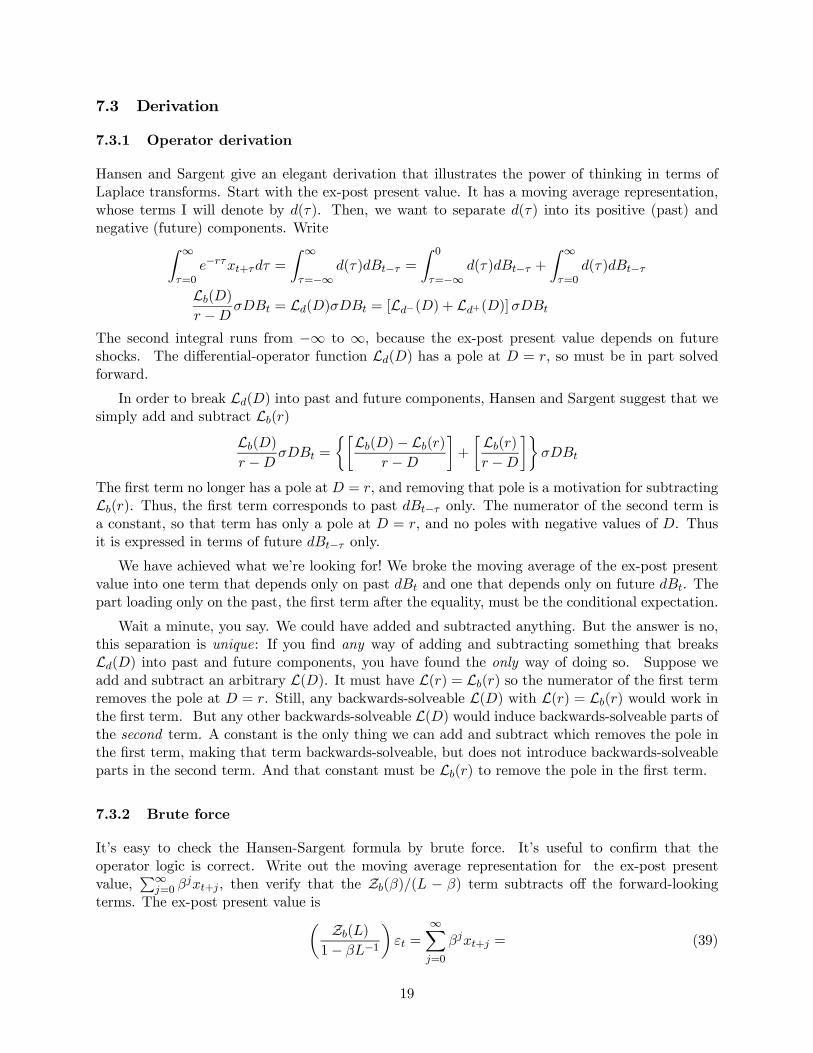
7.3 Derivation

7.3.1 Operator derivation

Hansen and Sargent give an elegant derivation that illustrates the power of thinking in terms of

Laplace transforms. Start with the ex-post present value. It has a moving average representation,

whose terms I will denote by (). Then, we want to separate () into its positive (past) and

negative (future) components. WriteZ ∞

=0

−+ =Z ∞

=−∞()− =

Z 0

=−∞()− +

Z ∞

=0

()−

L() −

= L() = [L−() + L+()]

The second integral runs from −∞ to ∞, because the ex-post present value depends on futureshocks. The differential-operator function L() has a pole at = , so must be in part solved

forward.

In order to break L() into past and future components, Hansen and Sargent suggest that wesimply add and subtract L()

L() −

=

½∙L()− L() −

¸+

∙ L() −

¸¾

The first term no longer has a pole at = , and removing that pole is a motivation for subtracting

L(). Thus, the first term corresponds to past − only. The numerator of the second term is

a constant, so that term has only a pole at = , and no poles with negative values of . Thus

it is expressed in terms of future − only.

We have achieved what we’re looking for! We broke the moving average of the ex-post present

value into one term that depends only on past and one that depends only on future . The

part loading only on the past, the first term after the equality, must be the conditional expectation.

Wait a minute, you say. We could have added and subtracted anything. But the answer is no,

this separation is unique: If you find any way of adding and subtracting something that breaks

L() into past and future components, you have found the only way of doing so. Suppose we

add and subtract an arbitrary L(). It must have L() = L() so the numerator of the first termremoves the pole at = . Still, any backwards-solveable L() with L() = L() would work inthe first term. But any other backwards-solveable L() would induce backwards-solveable parts ofthe second term. A constant is the only thing we can add and subtract which removes the pole in

the first term, making that term backwards-solveable, but does not introduce backwards-solveable

parts in the second term. And that constant must be L() to remove the pole in the first term.

7.3.2 Brute force

It’s easy to check the Hansen-Sargent formula by brute force. It’s useful to confirm that the

operator logic is correct. Write out the moving average representation for the ex-post present

value,P∞

=0 + , then verify that the Z()( − ) term subtracts off the forward-looking

terms. The ex-post present value isµ Z()

1− −1

¶ =

∞X=0

+ = (39)

19

=

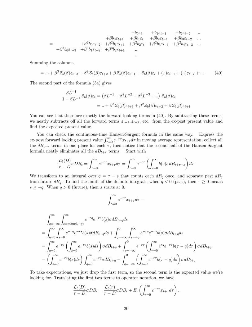
+0 +1−1 +2−2

+0+1 +1 +2−1 +3−2

+20+2 +21+1 +22 +23−1 +24−3

+30+3 +31+2 +32+1

Summing the columns,

= + 3Z()+3 + 2Z()+2 + Z()+1 +Z() + ()−1 + ()−2 + (40)

The second part of the formula (34) gives

−1

1− −1Z() =

¡−1 + 2−2 + 3−3 +

¢Z()

= + 3Z()+3 + 2Z()+2 + Z()+1

You can see that these are exactly the forward-looking terms in (40). By subtracting these terms,

we neatly subtracts off all the forward terms +1 +2, etc. from the ex-post present value and

find the expected present value.

You can check the continuous-time Hansen-Sargent formula in the same way. Express the

ex-post forward looking present valueR∞=0

−+ in moving average representation, collect allthe − terms in one place for each , then notice that the second half of the Hansen-Sargent

formula neatly eliminates all the + terms. Start with

L() −

=

Z ∞

=0

−+ =Z ∞

=0

−µZ ∞

=0

()+−

¶

We transform to an integral over = − that counts each once, and separate past

from future . To find the limits of the definite integrals, when 0 (past), then ≥ 0 means ≥ −. When 0 (future), then starts at 0.Z ∞

=0

−+ =

=

Z ∞

=−∞

Z ∞

=max(0−)−−()+

=

Z ∞

=0

Z ∞

=0

−−()++

Z 0

=−∞

Z ∞

=−−−()+

=

Z ∞

=0

−µZ ∞

=0

−()¶+ +

Z 0

=−∞−

µZ ∞

=0

−( − )

¶+

=

µZ ∞

=0

−()¶Z ∞

=0

−+ +

Z 0

=−∞

µZ ∞

=0

− ( − )

¶+

To take expectations, we just drop the first term, so the second term is the expected value we’re

looking for. Translating the first two terms to operator notation, we have

L() −

=L() −

+

µZ ∞

=0

−+¶

20

8 Integration and cointegration

So far, I have assumed that the series is stationary in levels. We study differences because

that is more convenient in continuous time. Here I take up the possibility that contains unit

roots; that is stationary but is not. I describe the transformation from differences to levels,

and the unit root and cointegrated representations of difference-stationary series.

8.1 Difference-stationary series

So far, we have been looking at differenced specifications simply because the differential operator

is more convenient in continuos time, though the level of the series is stationary, with the AR(1)

= − + as the canonical example. Often, we will model series whose differences

are stationary, but the levels are not, such as itself. Hence it’s worth writing down what

specifications based purely on differences look like.

The moving average is

= L()

=

Z ∞

=0

()− +

As before, I assume that () has a function at (0) = 1 to generate the Laplace transform L().Reiterating, we normalize so a unit shock has a unit effect on

lim→∞

L() = 1

A corresponding “autoregressive” representation is

L()−1 =

We make sense of these expressions with the usual manipulations. For example, a first-order

polynomial model is

= +

+

Its moving average representation can be written

=

µ1 +

−

+

¶

= ( − )

µZ ∞

=0

−−

¶+

The autoregressive representation is

+

+ = µ

1 +−

+

¶ =

= −(− )

µZ ∞

=0

−−

¶+

Here you see that we forecast future changes using past changes − , as we normally would runan autoregression in first differences for series like stock returns or GDP growth.

21

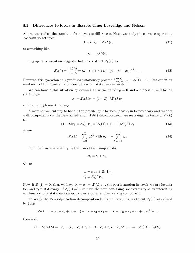
8.2 Differences to levels in discrete time; Beveridge and Nelson

Above, we studied the transition from levels to differences. Next, we study the converse operation.

We want to get from

(1− ) = Z() (41)

to something like

= Z()

Lag operator notation suggests that we construct Z() as

Z() =Z()

1− = 0 + (0 + 1)+ (0 + 1 + 2)

2 + (42)

However, this operation only produces a stationary process ifP∞

=0 = Z(1) = 0. That condition

need not hold. In general, a process (41) is not stationary in levels.

We can handle this situation by defining an initial value 0 = 0 and a process = 0 for all

≤ 0. Now = Z() = (1− )−1Z()

is finite, though nonstationary.

A more convenient way to handle this possibility is to decompose in to stationary and random

walk components via the Beveridge-Nelson (1981) decomposition. We rearrange the terms of Z()

as

(1− ) = Z() = [Z(1) + (1− )Z()] (43)

where

Z() =

∞X=0

with = −

∞X=+1

(44)

From (43) we can write as the sum of two components,

= +

where

= −1 +Z(1)

= Z()

Now, if Z(1) = 0, then we have = = Z() , the representation in levels we are looking

for, and is stationary. If Z(1) 6= 0, we have the next best thing; we express as an interestingcombination of a stationary series plus a pure random walk component.

To verify the Beveridge-Nelson decomposition by brute force, just write out Z() as defined

by (44):

Z() = −(1 + 2 + 3 + )− (2 + 3 + 4 + )− (3 + 4 + 5 + )2 −

then note

(1− )Z() = −0 − (1 + 2 + 3 + ) + 0 + 1+ 22 + = −Z(1) +Z()

22

Since the {} are square summable, so are the {} This is a key observation, Z() defines a

level-stationary process.

In operator notation, the decomposition (43) consists of just adding and subtracting Z(1)

(1− ) = Z() = Z(1) + (1− )

∙Z()−Z(1)

1−

¸ (45)

Then, we define Z() by

Z() =Z()−Z(1)

1−

to arrive at (43). This looks too easy — could you add and subtract anything, and multiply and

divide by (1 − )? But the fact that makes it work is that Z() = [Z()−Z(1)] (1 − ) is a

legitimate lag polynomial of a stationary process. All its poles lie outside the unit circle. (Following

usual practice, I do not normalize so Z(0) = 1.)

The Beveridge-Nelson trend has the property

= lim→∞

(+) (46)

which follows simply from the fact that is stationary so lim→∞+ = 0. This can also be

used as the defining property to derive the Beveridge-Nelson decomposition, which is a longer but

more satisfying since you construct the answer rather than verify it. Thinking in this way, we can

derive the Beveridge-Nelson decomposition as a case of the Hansen-Sargent formula (35) evaluated

at = 1:

= lim→∞

(+) = +

∞X=1

∆+ = +

µZ(1)−Z()

1−

¶

(1− ) = (1− )Z() + (1− )

µZ(1)−Z()

1−

¶ = Z(1)

Defining as detrended ,

= −

(1− ) = (1− ) + (1− )

(1− ) = [Z() +Z(1)]

8.3 Differences to levels in continuous time

The same operations have natural analogues in continuous time. Before, we found the differenced

moving average representation of a level-stationary series, in (24). Now we want to ask the converse

question. Suppose you have a differential representation,

= L()

How do you find L() or () in = L()? (47)

The fly in the ointment, as in discrete time, is that the process may not be stationary in

levels, so the latter integral doesn’t make sense. As a basic example, if you start with simple

Brownian motion

=

23

you can’t invert that to

= =

Z ∞

=0

−

because the latter integral blows up. For this reason, we usually express the level of pure Brownian

motion as an integral that only looks back to an initial level,

= 0 +

Z

=0

− = 0 + ( −0)

As in this example, we can ignore the nonstationarity, use (47) directly, and think of a nonstationary

process that starts at time 0 with = 0 for all 0. (Hansen and Sargent (1993), last

paragraph.)

Alternatively, we can handle this situation as in discrete time, with the continuous-time Beveridge-

Nelson decomposition that isolates the nonstationarity to a pure random walk component. We

rearrange the terms of L(),

= L() = [L(0) +L()] (48)

I’ll show in a moment how to construct L() , and verify that it is the differential-operator functionof a valid stationary process. Once that’s done, though, we can write this last equation as

= +

and hence

= +

where is a pure random walk

= L(0)

and is stationary in levels,

= L()

Now, if L(0) = 0 we have = stationary. If L(0) 6= 0, then we isolate the nonstationarityto a pure random walk component and put all the dynamics in a level-stationary stochastically

detrended component

Now, how do we construct L() given L()? The operator derivation is nearly trivial. Byconstruction,

L() = L(0) +

∙L()− L(0)

¸

Therefore, we just define

L() = L()− L(0)

(49)

Adding and subtracting L(0) and multiplying and dividing by looks artificial, but the key is

that (L()− L(0)) is a valid level-stationary process, since −L(0) removes the pole at 0.Equivalently, it produces a new difference operator function L∗() = L() − L(0), which doeshave the property L∗(0) = 0 and hence L() = L∗() is a proper level-stationary process.

We can construct the terms () by integrating ()

() = −Z ∞

=

()

24

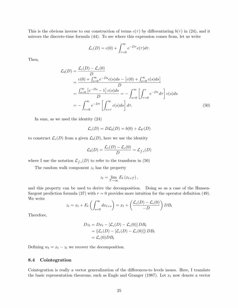
This is the obvious inverse to our construction of terms () by differentiating () in (24), and it

mirrors the discrete-time formula (44). To see where this expression comes from, let us write

L() = (0) +

Z ∞

=0

−()

Then,

L() = L()− L(0)

=(0) +

R∞=0

−()− £(0) + R∞=0

()¤

=

R∞=0

£− − 1¤ ()

= −

Z ∞

=0

∙Z

=0

−

¸()

= −Z ∞

=0

−

∙Z ∞

=

()

¸ (50)

In sum, as we used the identity (24)

L() = L() = (0) + L0()

to construct L() from a given L(), here we use the identity

L() = L()− L(0)

= L ()where I use the notation L () to refer to the transform in (50)

The random walk component has the property

= lim→∞

(+ )

and this property can be used to derive the decomposition. Doing so as a case of the Hansen-

Sargent prediction formula (37) with = 0 provides more intuition for the operator definition (49).

We write

= +

µZ ∞

=0

+

¶= +

µL()− L(0)−

¶

Therefore,

= − [L()− L(0)]

= {L()− [L()− L(0)]}

= L(0)

Defining = − we recover the decomposition.

8.4 Cointegration

Cointegration is really a vector generalization of the differences-to levels issues. Here, I translate

the basic representation theorems, such as Engle and Granger (1987). Let now denote a vector

25

of time series, and a vector of independent standard Brownian motions. The moving

average representations such as

=

Z ∞

=0

() −

=

µZ ∞

=0

() −

¶+

or in operator notation

= L()

= L() (51)

represent matrix operations. with L() and denoting × matrices.

For a scalar, the level/difference issue is whether L(0) = 0 or not. For a vector, we have theadditional possibility that L(0) may be nonzero but not full rank. In that case, the elements of are cointegrated. To keep the discussion simple I will mostly consider the case = 2, and

=£1 2

¤0

Cointegrated series have a common trend representation: If L(0) has rank 1, then we can writeL(0) = 0 (52)

where and are 2 × 1 vectors. Building on the Beveridge-Nelson decomposition (48), define ascalar random walk component ,

= 0

and we can write the two components of as a sum of this shared random walk component and

stationary components,

= +

i.e. ∙12

¸=

∙12

¸ +

∙12

¸ (53)

To derive this representation in operator notation, we proceed exactly as we did in deriving the

Beveridge-Nelson decomposition, interpreting the symbols as matrices, and introducing L(0) = 0

at the right time. From (51),

= L(0) +

∙L()− L(0)

¸

= 0 +L()

= +L()

or, in levels

= + L()

The cointegrating vector gives the linear combination of that is stationary in levels, though

the individual components of are not. Since L(0) = 0 is singular by assumption, we can find such that 0 = 0, and 0L(0) = 0, and we can find a such that 0 = 0 and L(0) = 0.

Then, from (53),

0 = 0

26

i.e., 0 is stationary. To get there directly, we can just write

= 0 +L()

0 =¡0¢0 + 0L()

0 = 0L()

0 = 0L()

The error-correction representation is also very useful. For example, forecasting regressions of

stock returns and dividend growth on dividend yields, or consumption and income growth on the

consumption / income ratio are good examples of useful error-correction representations.

A useful form of the error correction representation is

= −¡0

¢+

∙Z ∞

=0

−() −

¸+

Here is a 2× 1 vector which shows how the lagged cointegrating vector affects changes in each ofthe two differences. I allow extra stationary components in the middle term, expressed as moving

averages or “serially correlated errors” in discrete-time parlance. We could also follow the discrete-

time VAR literature and write these as lags of which help to forecast . The cointegrated

AR(1) is a useful special case, in which the middle term is missing. Finally, we have the shock

term.

In operator notation, this error correction representation is

= −¡0

¢+ L() (54)

The cointegrated AR(1) is the special case L() = .

Applying 0 to both sides, the cointegrating vector itself follows

¡0

¢= − ¡0¢ ¡0¢+ 0L()

Note 0 is a scalar (in general a full-rank) matrix. Therefore, the scalar process 0 is stationaryin levels, and has the moving-average representation

(0) =1

+ 00L() (55)

For the cointegrated AR(1) special case, this is just a scalar AR(1).

Now, let’s connect the error correction representation to the above moving-average characteri-

zations. We can substitute (55) back in to (54) to obtain the moving average differential operator

L(), =

µ − 0

+ 0

¶L() = L()

Since L(0) = , this moving average operator obeys

L(0) = − (0)−10

This is a rank 1 idempotent matrix, confirming the condition (52) that defines cointegration, and

generalizing the usual special cases L(0) = 0 (stationary in levels) and L(0) = (stationary in

differences.) Furthermore,

0L(0) = 0¡ − (0)−10

¢= 0

L(0) =¡ − (0)−10

¢ = 0

27

so the cointegrating vector defined by the error-correction mechanism is the same resulting from

the condition 0L(0) = 0

9 Summary

• Basic operators = −

=1

= −; = − log()

• Lag operators, differential operators, Laplace transforms, moving average representation

=

∞X=0

− = Z(); Z() =

∞X=0

; 0 = 1

=

Z ∞

=0

()− = L(); L() =Z ∞

=0

−() ; (0) = 1

• The AR(1)

+1 = + ⇒ =

∞X=0

−

= −+ ⇒ =

Z ∞

=0

−−

• Operators and inverting the AR(1)

(1− ) = ⇒ =1

1− =

⎛⎝ ∞X=0

⎞⎠

( + ) = ⇒ =1

+ =

µZ ∞

=0

−−

¶1

• Forward-looking operators

kk 1⇒µ

1

1−

¶ = −

µ−1−1

1− −1−1

¶ = −

⎛⎝ ∞X=1

−−

⎞⎠ = −∞X=1

−+

kk 0⇒ 1

− = −

µZ ∞

=0

−+

¶ = −

Z ∞

=0

−+

• Moving averages and moments.

2 () =

Z ∞

=0

2()2

( −) =Z ∞

=0

()(+ )2

() =

Z ∞

=−∞(− ) = L()L(−)2

28

( −) =1

2

Z ∞

−∞() =

1

2

Z ∞

−∞L()L(−)2

• Polynomial models and autoregressive representations

=( + 1) ( + 2)

( + 1) ( + 2)( + 3)

Moving average in partial fractions form

=

∙

+ 1+

+ 2+

+ 3+

¸

Autoregressive form ∙ ++

+ 1+

+ 2+

¸ =

• “AR(2)” =

( + 1)

( + 1) ( + 2)

Moving average

=1

1 − 2

µ1 − 1

+ 1− 2 − 1

+ 2

¶

=1 − 1

1 − 2

Z ∞

=0

−1− +2 − 1

2 − 1

Z ∞

=0

−2−

Autoregression ∙ + (1 + 2 − 1) +

(1 − 1)(1 − 2)

+ 1

¸ =

= − [(1 + 2)− 1]−µ(1 − 1)(1 − 2)

Z ∞

=0

−1−¶+

• Moving average representations for differences.

(1− ) = Z() = (1− )Z() = [1 +Z∆()]

The representation:

=

µZ ∞

=0

()−

¶+

= L()

Finding L() from L() :

L() = L() = 1 + L0()

=

µZ ∞

=0

0()−

¶+

29

The AR(1):

=

+ =

µ1−

+

¶

= −µZ ∞

=0

−−

¶+

Polynomials:

L() = 1− 1

+ 1− 2

+ 2−

• Impulse-response functions and multipliers

( −−1)+ =

“ lim∆→0

(+∆ −) ” + = ()

meaning, if = + , then

= ()+ ()

Impact multiplier:

0 = Z(0) = 1

(0) = lim→∞

[L()] = 1(0) = lim

→∞[L()] = 1

Final multiplier:

∞ = Z(∞)(∞) = lim

→0[L()]

These should be zero for a stationary .

Cumulative response ofR∞=0

+ :

Z(1) =

∞X=0

L(0) =Z ∞

=0

()

Cumulative response of =R∞=0

+ :

Z(1) =

∞X=0

L(0) = 1 +Z ∞

=0

()

These should be zero for a stationary .

30

• Hansen-Sargent prediction formulas

∞X=0

+ =

µZ()− Z()

−

¶

∞X=1

−1+ =µZ()−Z()

−

¶

( −−1)∞X=0

+ = Z()

Z ∞

=0

−+ =µL()− L()

−

¶

“ lim∆→0

(+∆ −) ”

Z ∞

=0

−+ = L()

• Difference-stationary processes

= L()

=

Z ∞

=0

()− +

Polynomial example. In moving average form:

= +

+

=

µ1 +

−

+

¶

= ( − )

µZ ∞

=0

−−

¶+

In autoregressive form:

+

+ = µ

1 +−

+

¶ =

= −(− )

µZ ∞

=0

−−

¶+

• Transforming from differences to levels, Beveridge-Nelson decompositions.

Z() = Z(1) + (1− )Z(); = −∞X

=+1

implies

= + ;

(1− ) = Z(1); = Z()

31

In continuous time,

= L() = [L(0) +L()]

implies

= + ;

= L(0); = L()

Constructing L()

L() = L()− L(0)

() = −Z ∞

=

()

has the “trend” property

= lim→∞

(+ ) = +

Z ∞

=0

+

• Cointegration. Given the moving average representation,

= L()

are cointegrated if L(0) has rank less than . Then

L(0) = 0

and there exist :

0 = 0L(0) = 0; 0 = L(0) = 0

The common trend representation

= 0

= +

The cointegrating vector 0 = 0 is stationary.

The error correction representation is

= −¡0

¢+ L()

32

10 References

Beveridge, Stephen, and Charles R. Nelson, 1981, “A new approach to decomposition of economic

time series into permanent and transitory components with particular attention to measure-

ment of the ’business cycle’,” Journal of Monetary Economics 7, 151-174.

http://dx.doi.org/10.1016/0304-3932(81)90040-4

Cochrane, John H., 2005a, Asset Pricing: Revised Edition. Princeton: Princeton University Press

http://press.princeton.edu/titles/7836.html

Cochrane, John H., 2005b, “Time Series for Macroeconomics and Finance” Manuscript, University

of Chicago,

http://faculty.chicagobooth.edu/john.cochrane/research/papers/time_series_book.pdf

Cochrane, John H., 2012, “A Continous-Time Asset Pricing Model with Habits and Durability,”

Manuscript, University of Chicago

http://faculty.chicagobooth.edu/john.cochrane/research/papers/linquad_asset_price_example.pdf

Hansen, Lars Peter, and Thomas J. Sargent, 1991, “Prediction Formulas for Continuous-Time

Linear Rational Expectations Models” Chapter 8 of Rational Expectations Econometrics,

https://files.nyu.edu/ts43/public/books/TOMchpt.8.pdf

Hansen, Lars Peter, and Thomas .J. Sargent, 1980, “Formulating and Estimating Dynamic Linear

Rational-Expectations Models,” Journal of Economic Dynamics and Control 2, 7-46.

Hansen, Lars Peter, and Thomas J. Sargent, 1981, “A Note On Wiener-Kolmogorov Prediction

Formulas for Rational Expectations Models,” Economics Letters 8,: 255-260,

Heaton, John, 1993, “The Interaction Between Time-Nonseparable Preferences and Time Aggre-

gation,” Econometrica 61 353-385

http://www.jstor.org/stable/2951555

Engle, Robert F. and C. W. J. Granger, 1987, “Co-Integration and Error Correction: Represen-

tation, Estimation, and Testing,” Econometrica, 55, 251-276

33