HIERARCHICAL LINEARMODELS

NESTED DESIGNS

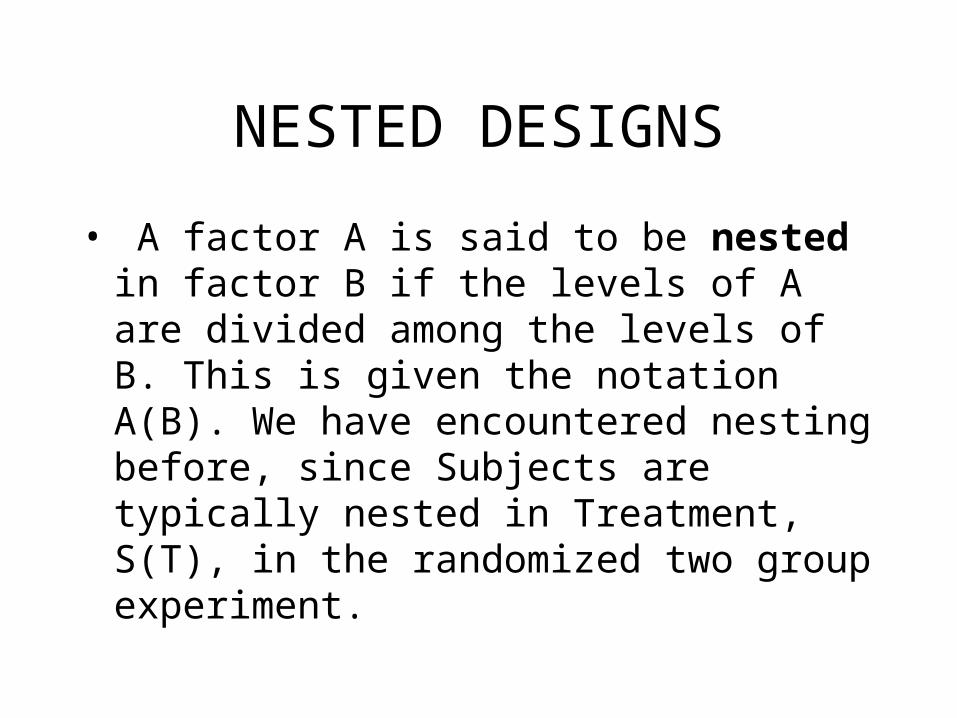
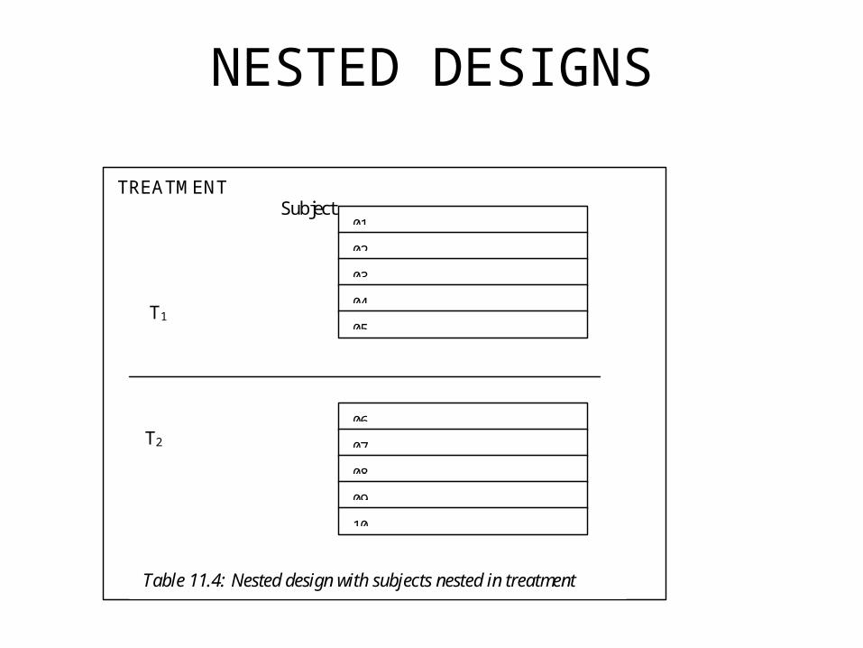
• A factor A is said to be nested in factor B if the levels of A are divided among the levels of B. This is given the notation A(B). We have encountered nesting before, since Subjects are typically nested in Treatment, S(T), in the randomized two group experiment.

NESTED DESIGNS

TREATMENT Subject

T1

T2

01

02

03

04

05

06

07

08

09

10

Table 11.4: Nested design with subjects nested in treatment

NESTED DESIGNS

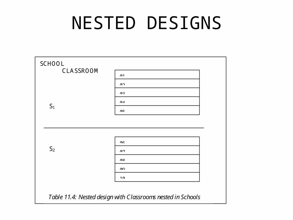
SCHOOLCLASSROOM

S1

S2

01

02

03

04

05

06

07

08

09

10

Table 11.4: Nested design with Classrooms nested in Schools

ANOVA TABLE

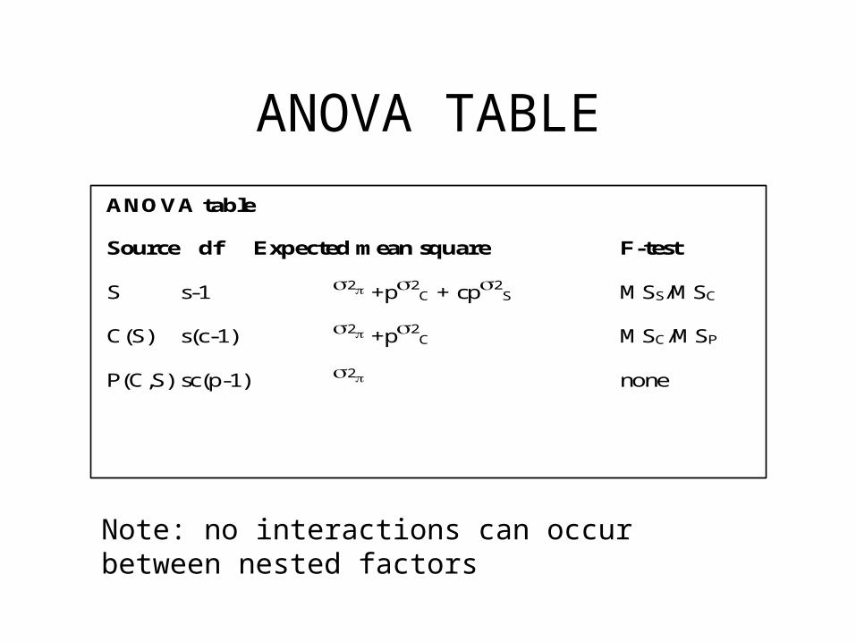
ANOVA table

Source df Expected mean square F-test

S s-1 2 +p2C + cp2

S MSS/MSC

C(S) s(c-1) 2 +p2C MSC/MSP

P(C,S) sc(p-1) 2 none

Note: no interactions can occur between nested factors

ESTIMATING VARIANCES

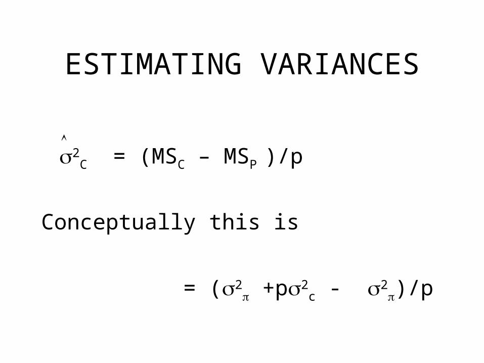
2C = (MSC – MSP )/p

Conceptually this is

= (2 +p2

c - 2)/p

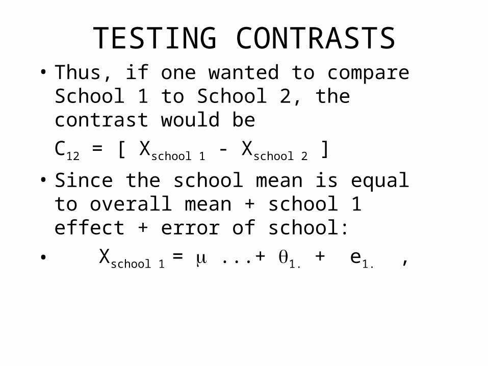
TESTING CONTRASTS• Thus, if one wanted to compare School 1 to

School 2, the contrast would be

C12 = [ Xschool 1 - Xschool 2 ]

• Since the school mean is equal to overall mean + school 1 effect + error of school:

• Xschool 1 = ...+ 1. + e1. ,

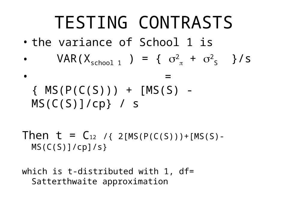
TESTING CONTRASTS• the variance of School 1 is

• VAR(Xschool 1 ) = { 2 + 2

S }/s

• = { MS(P(C(S))) + [MS(S) - MS(C(S)]/cp} / s

Then t = C12 /{ 2[MS(P(C(S)))+[MS(S)-MS(C(S)]/cp]/s}

which is t-distributed with 1, df= Satterthwaite approximation

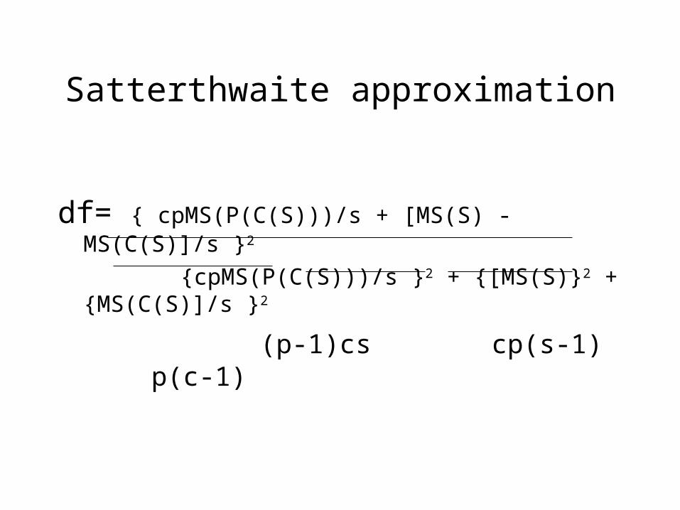
Satterthwaite approximation

df= { cpMS(P(C(S)))/s + [MS(S) - MS(C(S)]/s }2

{cpMS(P(C(S)))/s }2 + {[MS(S)}2 + {MS(C(S)]/s }2

(p-1)cs cp(s-1) p(c-1)

HLM - GLM differences

• GLM uses incorrect error terms in HLM designs– Multiple comparisons using GLM estimates

will be incorrect in many designs

• HLM uses estimates of all variances associated with an effect to calculate error terms

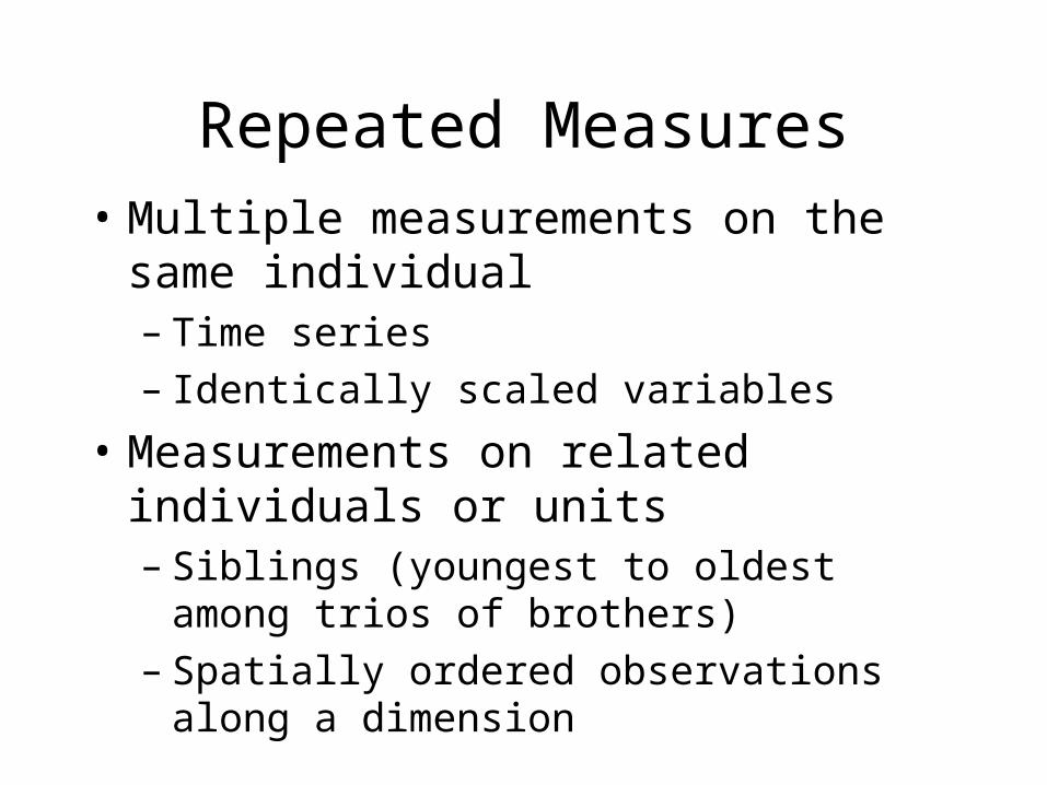
Repeated Measures• Multiple measurements on the same

individual – Time series– Identically scaled variables

• Measurements on related individuals or units– Siblings (youngest to oldest among trios of

brothers)– Spatially ordered observations along a

dimension

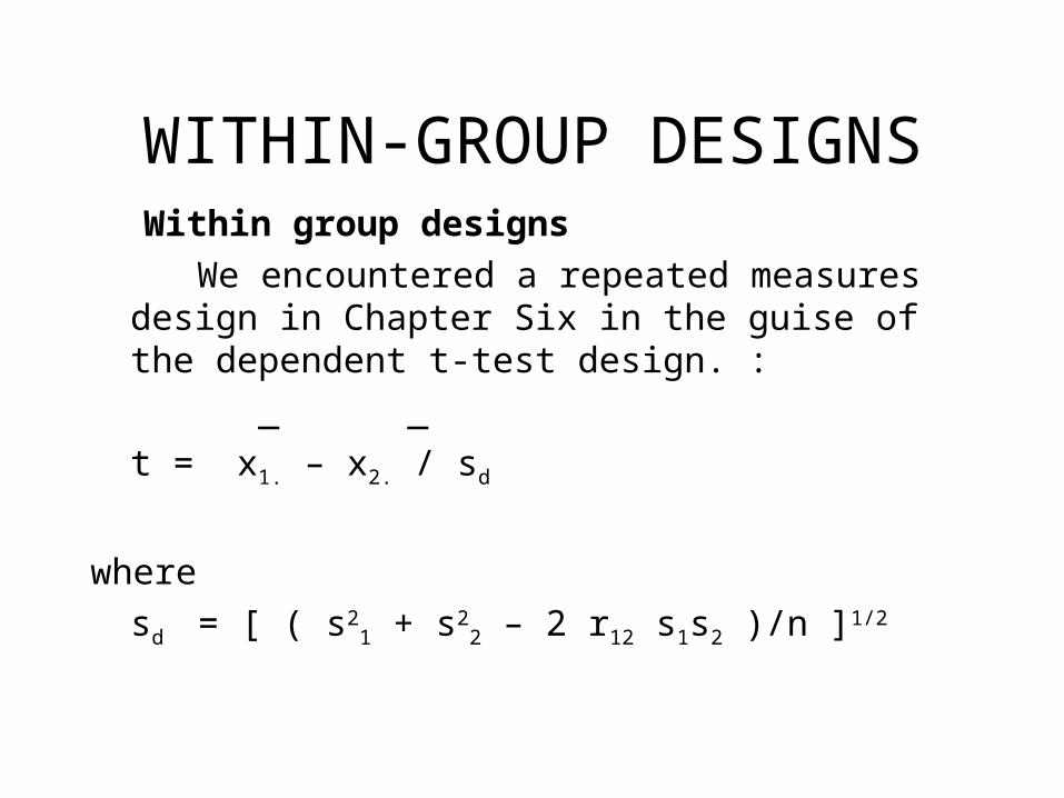
WITHIN-GROUP DESIGNSWithin group designs

We encountered a repeated measures design in Chapter Six in the guise of the dependent t-test design. :

_ _

t = x1. – x2. / sd

where

sd = [ ( s21 + s2

2 – 2 r12 s1s2 )/n ]1/2

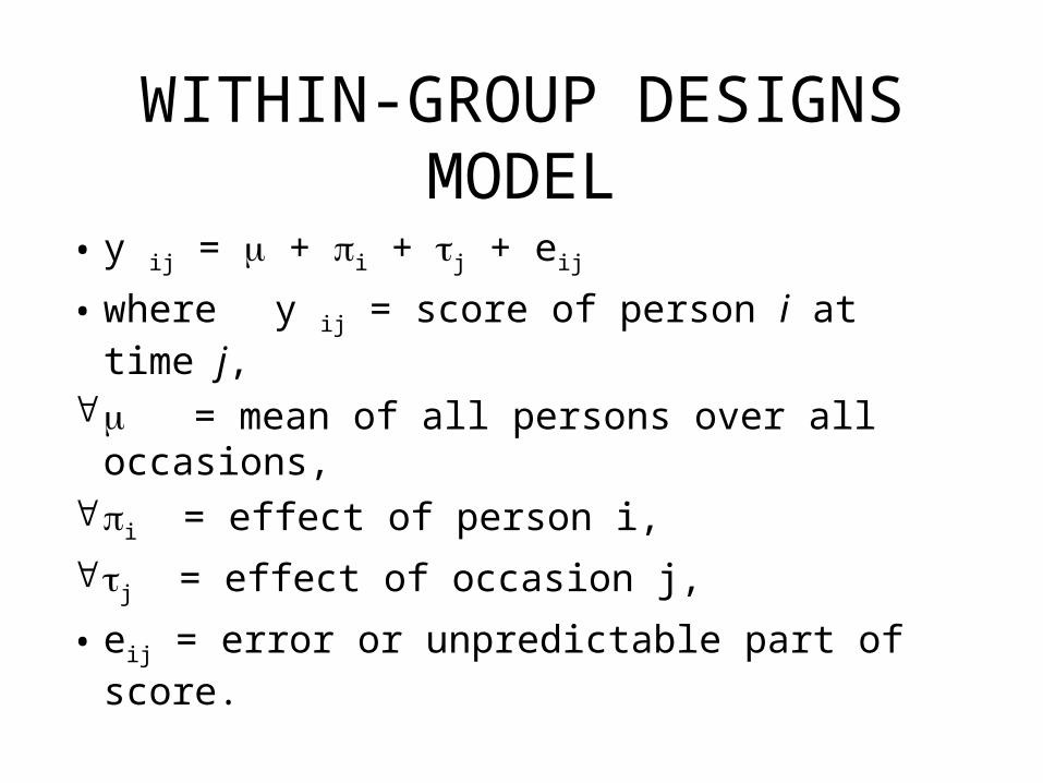
WITHIN-GROUP DESIGNSMODEL

• y ij = + i + j + eij

• where y ij = score of person i at time j,

= mean of all persons over all occasions, i = effect of person i,

j = effect of occasion j,

• eij = error or unpredictable part of score.

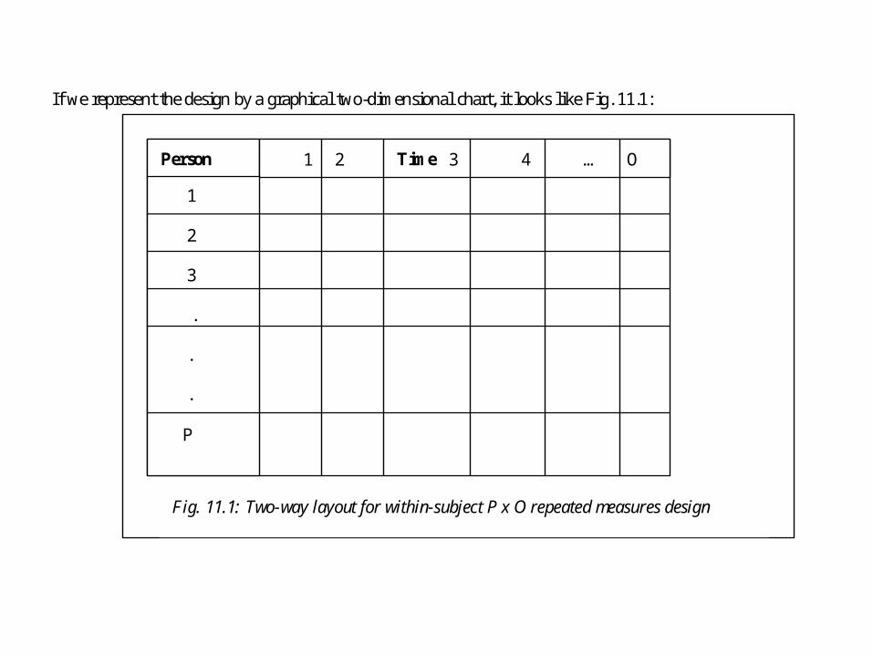
If we represent the design by a graphical two-dimensional chart, it looks like Fig. 11.1:

Person 1 2 Time 3 4 … O

1

2

3

.

.

.

P

Fig. 11.1: Two-way layout for within-subject P x O repeated measures design

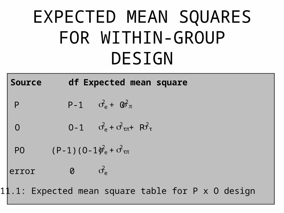
EXPECTED MEAN SQUARESFOR WITHIN-GROUP DESIGN

Source df Expected mean square

P P-1 2e + O2

O O-1 2e + 2

+ P2

PO (P-1)(O-1) 2e + 2

error 0 2e

Table 11.1: Expected mean square table for P x O design

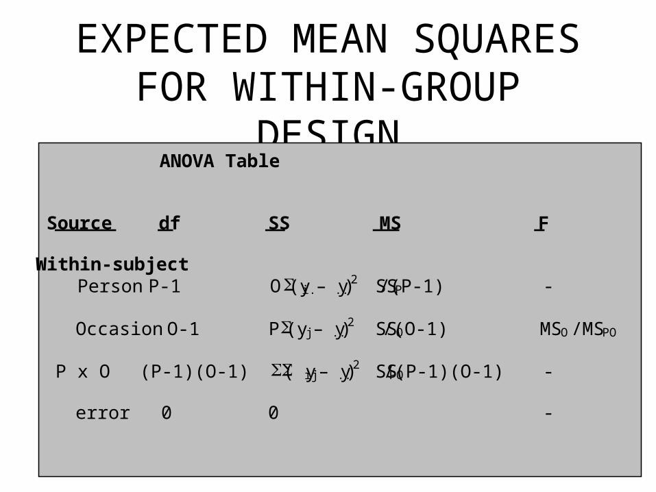
EXPECTED MEAN SQUARESFOR WITHIN-GROUP DESIGN

ANOVA Table

Source df SS MS F

Within-subject Person P-1 O(yi. – y..)

2 SSP/(P-1) -

Occasion O-1 P(y.j – y..)2 SSO/(O-1) MSO /MSPO

P x O (P-1)(O-1) ( yij – y..)2 SSPO/(P-1)(O-1) -

error 0 0 -

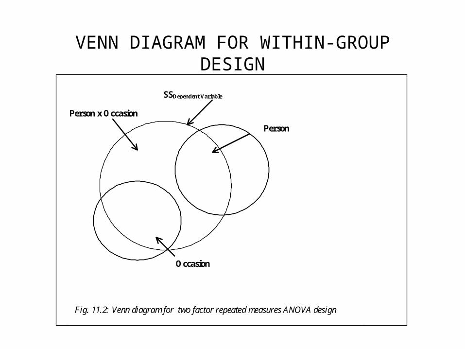
VENN DIAGRAM FOR WITHIN-GROUP DESIGN

SSe

SSDependent Variable

Person

Occasion

Person x Occasion

Fig. 11.2: Venn diagram for two factor repeated measures ANOVA design

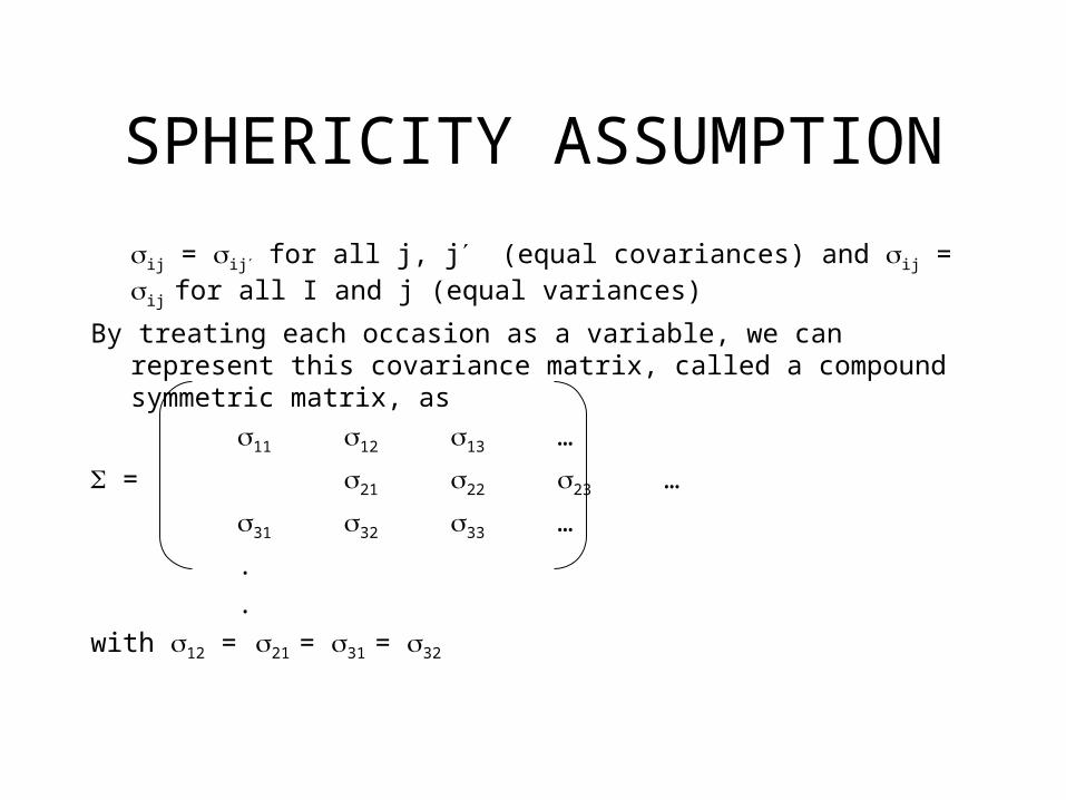
SPHERICITY ASSUMPTION

ij = ij for all j, j (equal covariances) and ij = ij for all I and j (equal variances)

By treating each occasion as a variable, we can represent this covariance matrix, called a compound symmetric matrix, as

11 12 13 …

= 21 22 23 …

31 32 33 …

.

.

with 12 = 21 = 31 = 32

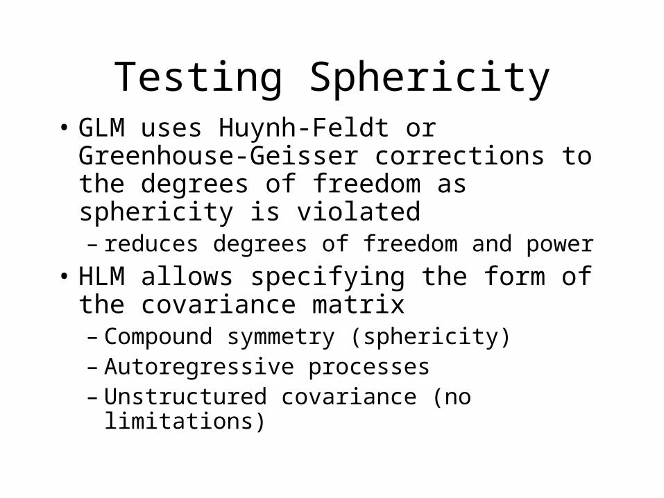
Testing Sphericity• GLM uses Huynh-Feldt or Greenhouse-

Geisser corrections to the degrees of freedom as sphericity is violated– reduces degrees of freedom and power

• HLM allows specifying the form of the covariance matrix– Compound symmetry (sphericity)– Autoregressive processes– Unstructured covariance (no limitations)

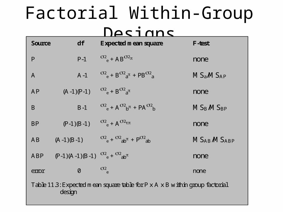
Factorial Within-Group DesignsSource df Expected mean square F-test

P P-1 2e + AB2 none

A A-1 2e + B2

a + PB2a MSa/MSAP

AP (A-1)(P-1) 2e + B2

a none

B B-1 2e + A2

b + PA2b MSB/MSBP

BP (P-1)(B-1) 2e + A2 none

AB (A-1)(B-1) 2e + 2

ab + P2ab MSAB/MSABP

ABP (P-1)(A-1)(B-1) 2e + 2

ab none

error 0 2e none

Table 11.3: Expected mean square table for P x A x B within group factorial design

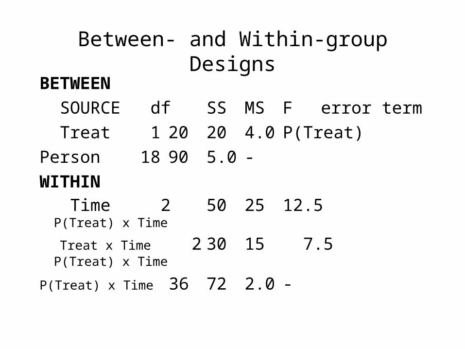
Between- and Within-group Designs

BETWEEN

SOURCE df SS MS F error term

Treat 1 20 20 4.0 P(Treat)

Person 18 90 5.0 -

WITHIN

Time 2 50 25 12.5 P(Treat) x Time

Treat x Time 2 30 15 7.5 P(Treat) x Time

P(Treat) x Time 36 72 2.0 -

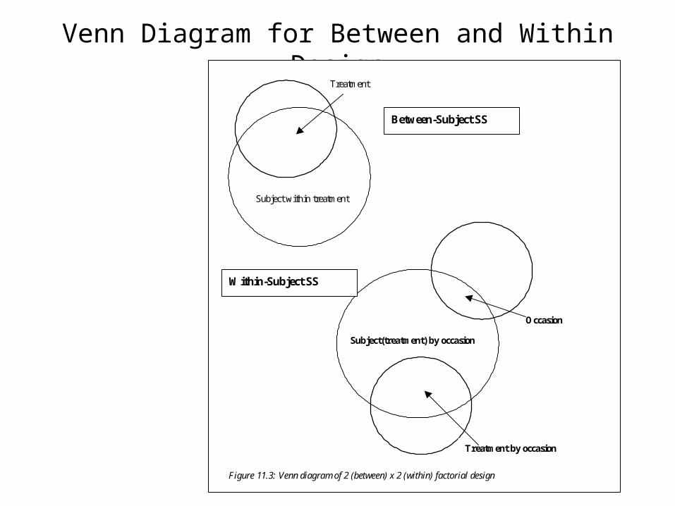
Venn Diagram for Between and Within Design

Between-Subject SS

Within-Subject SS

Treatment

Subject within treatment

Occasion

Treatment by occasion

Subject(treatment) by occasion

Figure 11.3: Venn diagram of 2 (between) x 2 (within) factorial design

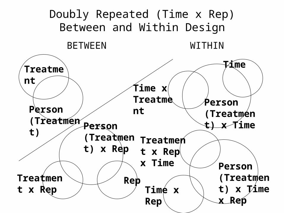
Doubly Repeated (Time x Rep) Between and Within Design

Treatment

Person (Treatment)

Time

Time x Treatment Person

(Treatment) x TimePerson

(Treatment) x Rep

Treatment x Rep

Rep

Person (Treatment) x Time x Rep

Treatment x Rep x Time

Time x Rep

BETWEEN WITHIN

HLM-GLM distinctions

• HLM correctly estimates contrasts for any hierarchical between-factors

• HLM correctly estimates all within-subject contrasts

• GLM does not estimate within-subject contrasts correctly

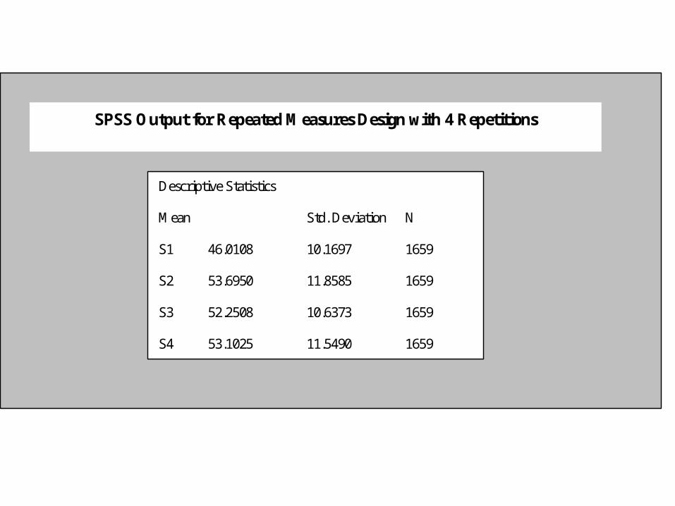
Descriptive Statistics

Mean Std. Deviation N

S1 46.0108 10.1697 1659

S2 53.6950 11.8585 1659

S3 52.2508 10.6373 1659

S4 53.1025 11.5490 1659

SPSS Output for Repeated Measures Design with 4 Repetitions

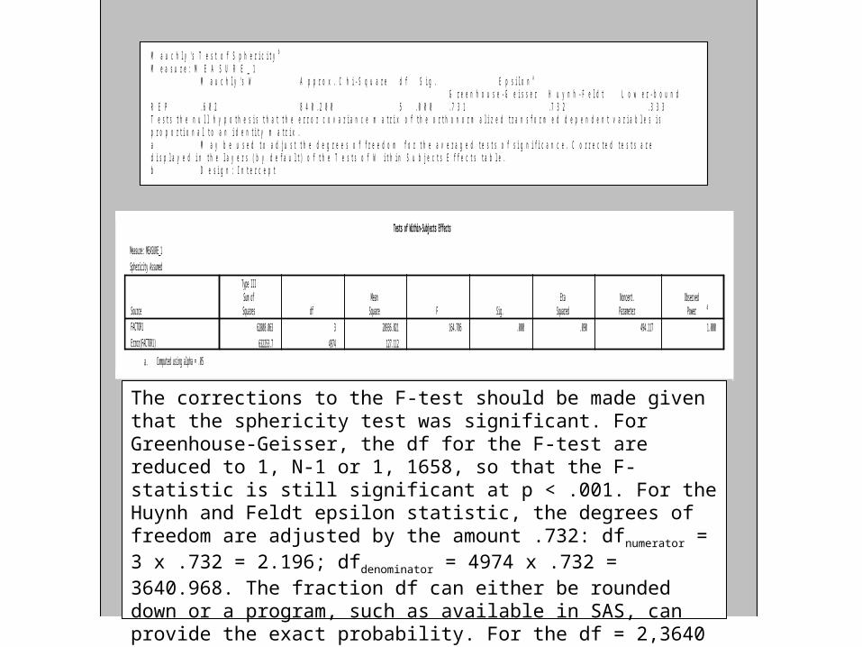
Measure: MEASURE_1

Sphericity Assumed

62808.063 3 20936.021 164.706 .000 .090 494.117 1.000

632253.7 4974 127.112

SourceFACTOR1

Error(FACTOR1)

Type IIISum of

Squares dfMean

Square F Sig.Eta

SquaredNoncent.Parameter

ObservedPower a

Tests of Within-Subjects Effects

Computed using alpha = .05a.

M a u c h l y ' s T e s t o f S p h e r i c i t y b

M e a s u r e : M E A S U R E _ 1M a u c h l y ' s W A p p r o x . C h i - S q u a r e d f S i g . E p s i l o n a

G r e e n h o u s e - G e i s s e r H u y n h - F e l d t L o w e r - b o u n dR E P . 6 0 2 8 4 0 . 2 0 0 5 . 0 0 0 . 7 3 1 . 7 3 2 . 3 3 3T e s t s t h e n u l l h y p o t h e s i s t h a t t h e e r r o r c o v a r i a n c e m a t r i x o f t h e o r t h o n o r m a l i z e d t r a n s f o r m e d d e p e n d e n t v a r i a b l e s i sp r o p o r t i o n a l t o a n i d e n t i t y m a t r i x .a M a y b e u s e d t o a d j u s t t h e d e g r e e s o f f r e e d o m f o r t h e a v e r a g e d t e s t s o f s i g n i f i c a n c e . C o r r e c t e d t e s t s a r ed i s p l a y e d i n t h e l a y e r s ( b y d e f a u l t ) o f t h e T e s t s o f W i t h i n S u b j e c t s E f f e c t s t a b l e .b D e s i g n : I n t e r c e p t

The corrections to the F-test should be made given that the sphericity test was significant. For Greenhouse-Geisser, the df for the F-test are reduced to 1, N-1 or 1, 1658, so that the F-statistic is still significant at p < .001. For the Huynh and Feldt epsilon statistic, the degrees of freedom are adjusted by the amount .732: dfnumerator = 3 x .732 = 2.196; dfdenominator = 4974 x .732 = 3640.968. The fraction df can either be rounded down or a program, such as available in SAS, can provide the exact probability. For the df = 2,3640 the F-statistic is still significant. Kirk (1996) discussed in detail various adjustments and recommends one by Collier, Baker, Mandeville, and Hayes (1967), but the computation is cumbersome; HLM analyses compute it.