Western Kentucky UniversityTopSCHOLAR®

Masters Theses & Specialist Projects Graduate School

5-2012

Continued Radicals and Cantor SetsThomas Tyler ClarkWestern Kentucky University, thomas.clark973@topper.wku.edu

Follow this and additional works at: http://digitalcommons.wku.edu/theses

Part of the Mathematics Commons

This Thesis is brought to you for free and open access by TopSCHOLAR®. It has been accepted for inclusion in Masters Theses & Specialist Projects byan authorized administrator of TopSCHOLAR®. For more information, please contact topscholar@wku.edu.

Recommended CitationClark, Thomas Tyler, "Continued Radicals and Cantor Sets" (2012). Masters Theses & Specialist Projects. Paper 1145.http://digitalcommons.wku.edu/theses/1145

CONTINUED RADICALS AND CANTOR SETS

A ThesisPresented to

The Faculty of the Department of MathematicsWestern Kentucky University

Bowling Green, Kentucky

In Partial FulfillmentOf the Requirements for the Degree

Master of Science

ByThomas Tyler Clark

May 2012

ACKNOWLEDGMENTS

I would like to thank my advisor, Dr. Tom Richmond, for his support through

the entire thesis process. He has been very patient and helpful during the research

and typing phases. Always lending a helping hand, his guidance has made this

research possible.

I am also very thankful to the other professors on my committee, Dr. John

Spraker and Dr. Dominic Lanphier. I appreciate their efforts in providing me with

feedback regarding the research and writing of this thesis. Furthermore, I would

like to thank Dr. Ferhan Atici for her information regarding difference equations

and measure theory.

Thank you to my friends and family for being supportive throughout the

entire process.

iii

CONTENTS

List of Figures v

List of Tables vi

Abstract vii

Chapter 1. Introduction 1

Chapter 2. Properties of Bridges and Gaps 13

Chapter 3. Thickness 20

Chapter 4. Measure 34

Chapter 5. Conclusion 40

Bibliography 42

iv

LIST OF FIGURES

1.1 Fluctuation in Function Versus Fluctuation in Tangent Line 4

1.2 Gaps and Bridges 12

1.3 Ordered Derivations 12

3.1 Middle Thirds Cantor Set 25

v

LIST OF TABLES

2.1 Gap Lengths of Cantor set generated by M = {1, 2} 19

3.1 Gap Lengths of Cantor set generated by M = {1, 3} 23

3.2 Thickness of Cantor Sets generated by continued radicals generated by M 27

3.3 Thickness of Cantor sets generated by continued radicals composed from{1, b} 28

3.4 Thickness of Cantor sets generated by continued radicals composed from{4, b} 29

3.5 Thickness of Cantor sets generated by continued radicals composed from{a, 50} 30

3.6 Minimum Number of Cantor sets generated by continued radicals composedfrom {a, b} required to guarantee an interval 32

3.7 Minimum Number of Cantor sets generated by continued radicals composedfrom {1, 4}, {5, 8}, and {6, 10} required to guarantee an interval 33

vi

CONTINUED RADICALS AND CANTOR SETS

Thomas Tyler Clark May 2012 42 Pages

Directed by: Tom Richmond, Dominic Lanphier, and John Spraker

Department of Mathematics and Computer Science Western Kentucky University

We examine the formation of sets homeomorphic to the ternary Cantor set by

continued radicals. We determine properties of bridges and gaps and calculate the

thickness of the Cantor set. From this we apply information from continued

fractions to continued radicals to obtain new results. We also consider the measure

of several Cantor sets.

vii

Chapter 1

Introduction

We define an Iterated Function System to be a finite set of contraction

mappings from a compact metric space onto itself. IFS’s are often associated with

fractals and their related image compression techniques. Commonly used examples

of IFS’s include infinite products, series, continued fractions, and continued radicals.

Mathematicians have been studying continued fractions for quite some time

with the phrase first being used in Wallis’ 1653 work titled, Arithmetica

infinitorum. Continued fractions are of the form,

x = a0 +b1

a1 + b2a2+

b3a3+...

,

where ai, bi+1 ∈ R for i ∈ N ∪ {0} Note that the most commonly studied continued

fractions have the property that ai, bi+1 ∈ Z+ ∪ {0} for i ∈ N ∪ {0}.

Continued radicals, although related to continued fractions, have received

notably less attention from researchers. Continued radicals are composed of a

sequence of nested radicals. A nested radical is of the form,√x0 +

√x1 +

√x2 + . . .+

√xn,

where xi ∈ R+ ∪ {0} for i ∈ N ∪ {0}, whereas a continued radical is of the form,

limn→∞

√x0 +

√x1 +

√x2 + . . .+

√xn.

Similarly, the most commonly studied continued radicals have xi ∈ Z+ for

i ∈ N ∪ {0}. However, it is necessary that xi > 0 for all i ∈ N ∪ {0} to make the

partial expressions be defined in R.

1

For ease of notation, we often represent nested radicals by√x0, x1, x2, . . . , xn

and continued radicals by√x0, x1, x2, . . ..

The following theorem, proven by Sizer[23], demonstrates the significance of

continued radicals.

Theorem 1.1. Any positive real number can be represented as a continued

radical√a0 +

√a1 + . . . where a0 ∈ N ∪ {0} and for i ≥ 1, ai ∈ {0, 1, 2}.

It is important to note that the above representation only yields positive real

numbers; however, multiplying by (−1) will give the negative real numbers, hence,

allowing us to represent any real number in this manner. This theorem

demonstrates the relevance of continued radicals. Prior to utilizing Theorem 1.1 to

construct real numbers, we must analyze the convergence of continued radicals. It

is necessary to consider the nested radicals, sometimes referred to as partial

expressions, that compose the continued radical and verify their convergence.

Laugwitz [16] and Sizer [23] have extensively considered the conditions for

convergence. Since our work entails studying continued radicals of the form

√a1, a2, . . . such that ai ∈ A where A is a specified finite set of nonnegative integers,

we need only consider the convergence results noted by Johnson and Richmond [15].

Theorem 1.2. If the sequence (ai)∞i=1 of nonnegative numbers is bounded

above, then√a1, a2, a3, . . . converges.

Consider the sequence (ai)∞i=1 = (n, n, . . .). We have that (ai)

∞i=1 is bounded

above. Thus, by Theorem 1.2, we have that φn =√n, n, n, . . . converges for any

nonnegative real number.

Proposition 1.3. We have that φn =1 +√

4n+ 1

2for n ∈ R+.

2

Proof. Note thatφn =

√n, n, . . .

=⇒ φ2n = n+

√n, n, . . .

= n+ φn

=⇒ φ2n − φn − n = 0.

By the quadratic equation, we get that φn =√n, n, . . . = 1+

√4n+12

. �

The following example demonstrates the use of Proposition 1.3 in constructing

the golden ratio.

Example 1.4. Consider√

1, 1, · · · = φ1 which converges by Theorem 1.2.

Then we have that by Proposition 1.3, φ1 =√

1, 1, . . . =1+√

4(1)+1

2= 1+

√5

2.

Although Theorem 1.2 is sufficient for our study, it is important to note that

the converse statement is not true. The following example was introduced by

Ramanujan in 1911. As noted by Borwein and de Barra [8], Ramanujan did not

consider the convergence of the continued radical but only to what they converged.

We will, however, consider the convergence.

Example 1.5 (Ramanujan). The continued radical√1 + 2

√1 + 3

√1 + 4 · · ·

=

√1 +

√22 +

√2432 +

√283442 + · · ·

=

√1!2 +

√2!21!2 +

√3!22!21!2 +

√4!23!22!21!2 + · · ·

converges to 3.

Lemma 1.6.

√1 + 2

√1 + 3

√1 + · · · converges.

Since 1!2, 2!21!2, 3!22!21!2, . . . is not bounded above, Theorem 1.2 does not

apply. Therefore, we must first prove that the continued radical actually converges.

3

Proof 1 of Lemma 1.6. Let an = (1!2! · · ·n!)2. We want to show that the

sequence P1 =√

1, P2 =√

1, (1!2!)2, P3 =√

1, (1!2!)2, (1!2!3!)2, . . . of partial

expressions converges. It is obvious that P1, P2, . . . increases. Since an increasing

sequence that is bounded above converges, it suffices to show that the sequence

P1, P2 of partial expressions is bounded above.

Let f(x) =√a1, a2, . . . , an−1, an + x. Then we have the following

f(0) =√a1, a2, . . . , an−1, an = Pn,

f(√an+1) =

√a1, a2, . . . , an−1, an +

√an+1 = Pn+1, and

f ′(x) =1

2n√a1, . . . , an + x

√a2, . . . , an + x, . . .

√an + x

.

Since 2n,√a1, . . . , an + x,

√a2, . . . , an + x, . . . ,

√an + x > 0 and

√a1, . . . , an + x,

√a2, . . . , an + x, . . . ,

√an + x are increasing in x, we have that

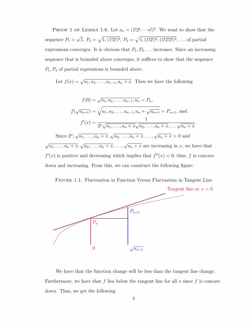
f ′(x) is positive and decreasing which implies that f ′′(x) < 0; thus, f is concave

down and increasing. From this, we can construct the following figure.

Figure 1.1. Fluctuation in Function Versus Fluctuation in Tangent Line

0

Pn

√an+1

Pn+1

Tangent line at x = 0

We have that the function change will be less than the tangent line change.

Furthermore, we have that f lies below the tangent line for all x since f is concave

down. Thus, we get the following

4

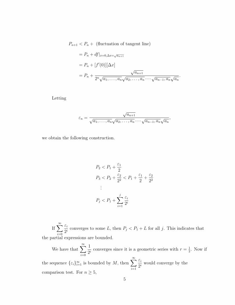
Pn+1 < Pn + (fluctuation of tangent line)

= Pn + df |x=0,∆x=√an+1

= Pn + [f ′(0)][∆x]

= Pn +

√an+1

2n√a1, . . . , an

√a2, . . . , an · · ·

√an−1, an

√an.

Letting

εn =

√an+1√

a1, . . . , an√a2, . . . , an · · ·

√an−1, an

√an,

we obtain the following construction.

P2 < P1 +ε1

2

P3 < P2 +ε2

22< P1 +

ε1

2+ε2

22

...

Pj < P1 +

j∑i=1

εi2i

If∞∑i=0

εi2i

converges to some L, then Pj < P1 + L for all j. This indicates that

the partial expressions are bounded.

We have that∞∑i=0

1

2iconverges since it is a geometric series with r = 1

2. Now if

the sequence {εi}∞i=1 is bounded by M , then∞∑i=1

εi2i

would converge by the

comparison test. For n ≥ 5,

5

εn =

√an+1√

a1, . . . , an√a2, . . . , an · · ·

√an−1, an

√an

=

√((n+ 1)!n!(n− 1)! · · · 2!1!)2

√a1, . . . , an

√a2, . . . , an · · ·

√an−2, an−1, an

√an−1, an

√(n!(n− 1)! · · · 2!1!)2

=(n+ 1)!

√a1, . . . , an

√a2, . . . , an · · ·

√an−2, an−1, an

√[(n− 1)!(n− 2)! · · · 2!1!)2 +

√an

<(n+ 1)!

√a1, . . . , an

√a2, . . . , an · · ·

√an−2, an−1, an[(n− 1)!(n− 2)! · · · 2!1!]

=(n+ 1)n

√a1, . . . , an

√a2, . . . , an · · ·

√an−2, an−1, an(n− 2)! · · · 2!1!

<(n+ 1)n

(n− 2)(n− 3)(n− 4)

=

(n+ 1

n− 2

)(n

n− 3

)(1

n− 4

)=

((n− 2) + 3

n− 2

)((n− 3) + 3

n− 3

)(1

n− 4

)=

(1 +

3

n− 2

)(1 +

3

n− 3

)(1

n− 4

)≤ 5.

(1.1)

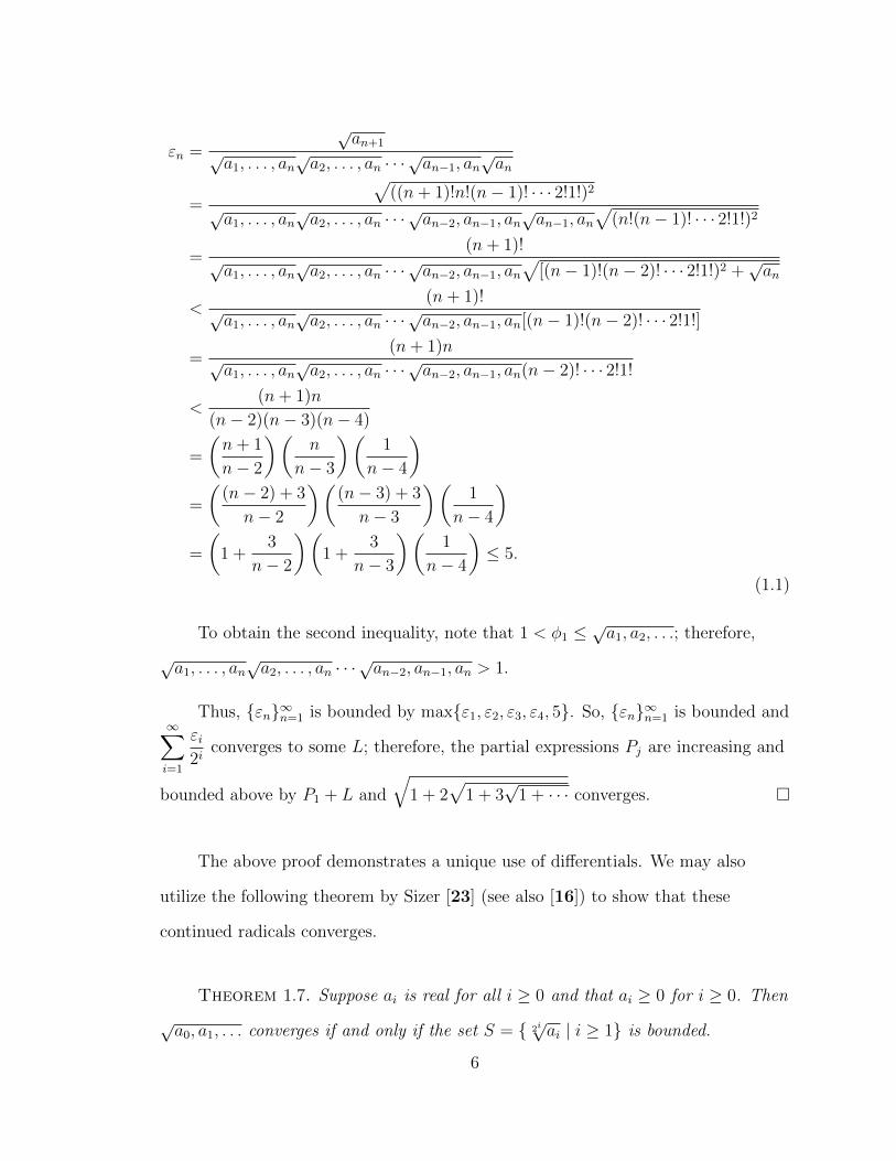
To obtain the second inequality, note that 1 < φ1 ≤√a1, a2, . . .; therefore,

√a1, . . . , an

√a2, . . . , an · · ·

√an−2, an−1, an > 1.

Thus, {εn}∞n=1 is bounded by max{ε1, ε2, ε3, ε4, 5}. So, {εn}∞n=1 is bounded and∞∑i=1

εi2i

converges to some L; therefore, the partial expressions Pj are increasing and

bounded above by P1 + L and

√1 + 2

√1 + 3

√1 + · · · converges. �

The above proof demonstrates a unique use of differentials. We may also

utilize the following theorem by Sizer [23] (see also [16]) to show that these

continued radicals converges.

Theorem 1.7. Suppose ai is real for all i ≥ 0 and that ai ≥ 0 for i ≥ 0. Then

√a0, a1, . . . converges if and only if the set S = { 2i

√ai | i ≥ 1} is bounded.

6

Proof 2 of Lemma 1.6. We first need to consider the convergence properties

of the right hand side. We will use Theorem 1.7 to accomplish this.

Let an = n!2(n− 1)!2(n− 2)!2 . . . 3!22!21!2. For n ≥ 4, we have the following

construction.

(n− 2)!(n− 3)! · · · 2!1! ≥ 2 > 1 +2

n− 1

=⇒ (n− 1)!(n− 2)! · · · 2!1! > (n− 1) + 2 = n+ 1

=⇒ n!(n− 1)!(n− 2)! · · · 2!1! > (n+ 1)!

=⇒ [n!(n− 1)!(n− 2!) · · · 2!1!]2 > (n+ 1)!n!(n− 1)! · · · 2!1!

=⇒ [n!(n− 1)!(n− 2!) · · · 2!1!]1

2n−1 > [(n+ 1)!n!(n− 1)! · · · 2!1!]12n

=⇒ 2n√an > 2n+1√an+1

Thus we have that the sequence

{ 2n√an} = { 2n

√n!2(n− 1)!2(n− 2)!2 . . . 3!22!21!2} is decreasing for n ≥ 4 and

therefore is bounded.

Hence,

√1 + 2

√1 + 3

√1 + 4 · · · converges. �

Thus, we have a sequence of nonnegative numbers that is not bounded above,

yet the continued radical formed by the sequence converges. This example

illustrates that the converse of Theorem 1.2 is not necessarily true.

Now that we have proven convergence, we can consider to what Ramanujan’s

continued radical converges. The proof below is related to a proof given by Sury

[25].

7

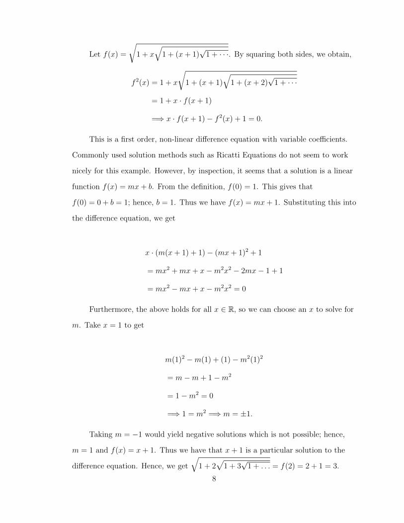
Let f(x) =

√1 + x

√1 + (x+ 1)

√1 + · · ·. By squaring both sides, we obtain,

f 2(x) = 1 + x

√1 + (x+ 1)

√1 + (x+ 2)

√1 + · · ·

= 1 + x · f(x+ 1)

=⇒ x · f(x+ 1)− f 2(x) + 1 = 0.

This is a first order, non-linear difference equation with variable coefficients.

Commonly used solution methods such as Ricatti Equations do not seem to work

nicely for this example. However, by inspection, it seems that a solution is a linear

function f(x) = mx+ b. From the definition, f(0) = 1. This gives that

f(0) = 0 + b = 1; hence, b = 1. Thus we have f(x) = mx+ 1. Substituting this into

the difference equation, we get

x · (m(x+ 1) + 1)− (mx+ 1)2 + 1

= mx2 +mx+ x−m2x2 − 2mx− 1 + 1

= mx2 −mx+ x−m2x2 = 0

Furthermore, the above holds for all x ∈ R, so we can choose an x to solve for

m. Take x = 1 to get

m(1)2 −m(1) + (1)−m2(1)2

= m−m+ 1−m2

= 1−m2 = 0

=⇒ 1 = m2 =⇒ m = ±1.

Taking m = −1 would yield negative solutions which is not possible; hence,

m = 1 and f(x) = x+ 1. Thus we have that x+ 1 is a particular solution to the

difference equation. Hence, we get

√1 + 2

√1 + 3

√1 + . . . = f(2) = 2 + 1 = 3.

8

We also need to consider some relations between continued radicals. First, we

have the following definition.

Definition 1.8. We say that 〈x1, x2, . . . , xn〉 ≤ 〈y1, y2, . . . , yn〉 coordinate-wise

if xi ≤ yi for all i ∈ {1, 2, . . . , n}.

This definition gives rise to the following Proposition by Johnson and

Richmond [15].

Proposition 1.9. If ai ≥ bi ≥ 0 for all i ∈ N, then

√a1, a2, . . . , ak ≥

√b1, b2, . . . , bk for all k ∈ N.

The converse of Proposition 1.9 does not hold.

Our main goals for studying continued radicals involve Cantor sets. Bartle and

Sherbert [7] give the following definition.

Definition 1.10. We define the Middle-Thirds Cantor set, C3, to be the

intersection of the sets Cn for n ∈ N, obtained by successive removal of open middle

thirds, starting with the unit interval [0, 1].

Note that the Middle-thirds Cantor set is C3 =⋂n∈Z+

Cn where I = [0, 1],

C0 = [0, 13] ∪ [2

3, 1] and Cn = [Cn−1] \

[∞⋃k=0

(1 + 3k

3n,2 + 3k

3n

)].

Johnson and Richmond [15] gives the following theorem regarding Cantor sets

formed by continued radicals.

Theorem 1.11. If m1 and m2 are natural numbers with m1 < m2, then the set

D = {√a1, a2, . . . | ai ∈ {m1,m2} ∀i ∈ N} is homeomorphic to the Middle-Thirds

Cantor set, C3.

9

It is important to note that this theorem does not take into consideration of

allowing m1 = 0. The Cantor sets from Theorem 1.11 will be the focus of this

thesis. A more extensive discussion of Theorem 1.11 is given in Chapter 2.

Now, we need to consider a key component making continued radicals IFS’s.

Definition 1.12. Let 〈M,ρ〉 be a metric space. If T : M →M , we say that T

is a contraction on M if there exists α ∈ (0, 1) such that ρ(T (x), T (y)) ≤ αρ(x, y),

for every x, y ∈M .

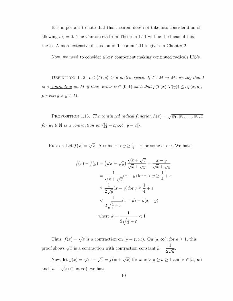
Proposition 1.13. The continued radical function h(x) =√w1, w2, . . . , wn, x

for wi ∈ N is a contraction on 〈[14

+ ε,∞), |y − x|〉.

Proof. Let f(x) =√x. Assume x > y ≥ 1

4+ ε for some ε > 0. We have

f(x)− f(y) =(√

x−√y) √x+

√y

√x+√y

=x− y√x+√y

=1√

x+√y

(x− y) forx > y ≥ 1

4+ ε

≤ 1

2√y

(x− y) for y ≥ 1

4+ ε

<1

2√

14

+ ε(x− y) = k(x− y)

where k =1

2√

14

+ ε< 1

Thus, f(x) =√x is a contraction on [1

4+ ε,∞). On [a,∞), for a ≥ 1, this

proof shows√x is a contraction with contraction constant k =

1

2√a

.

Now, let g(x) =√w +√x = f(w +

√x) for w, x > y ≥ a ≥ 1 and x ∈ [a,∞)

and (w +√x) ∈ [w,∞), we have

10

g(x)− g(y) = f(w +√x)− f(w +

√y)

≤ 1

2√w

(√x−√y)

=1

2√w

[f(x)− f(y)]

=1

4√wa

(x− y).

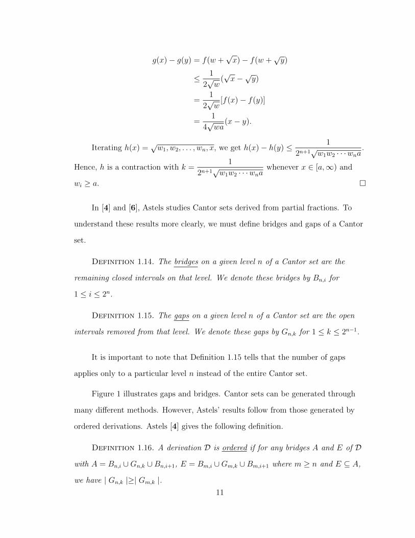
Iterating h(x) =√w1, w2, . . . , wn, x, we get h(x)− h(y) ≤ 1

2n+1√w1w2 · · ·wna

.

Hence, h is a contraction with k =1

2n+1√w1w2 · · ·wna

whenever x ∈ [a,∞) and

wi ≥ a. �

In [4] and [6], Astels studies Cantor sets derived from partial fractions. To

understand these results more clearly, we must define bridges and gaps of a Cantor

set.

Definition 1.14. The bridges on a given level n of a Cantor set are the

remaining closed intervals on that level. We denote these bridges by Bn,i for

1 ≤ i ≤ 2n.

Definition 1.15. The gaps on a given level n of a Cantor set are the open

intervals removed from that level. We denote these gaps by Gn,k for 1 ≤ k ≤ 2n−1.

It is important to note that Definition 1.15 tells that the number of gaps

applies only to a particular level n instead of the entire Cantor set.

Figure 1 illustrates gaps and bridges. Cantor sets can be generated through

many different methods. However, Astels’ results follow from those generated by

ordered derivations. Astels [4] gives the following definition.

Definition 1.16. A derivation D is ordered if for any bridges A and E of D

with A = Bn,i ∪Gn,k ∪Bn,i+1, E = Bm,i ∪Gm,k ∪Bm,i+1 where m ≥ n and E ⊆ A,

we have | Gn,k |≥| Gm,k |.11

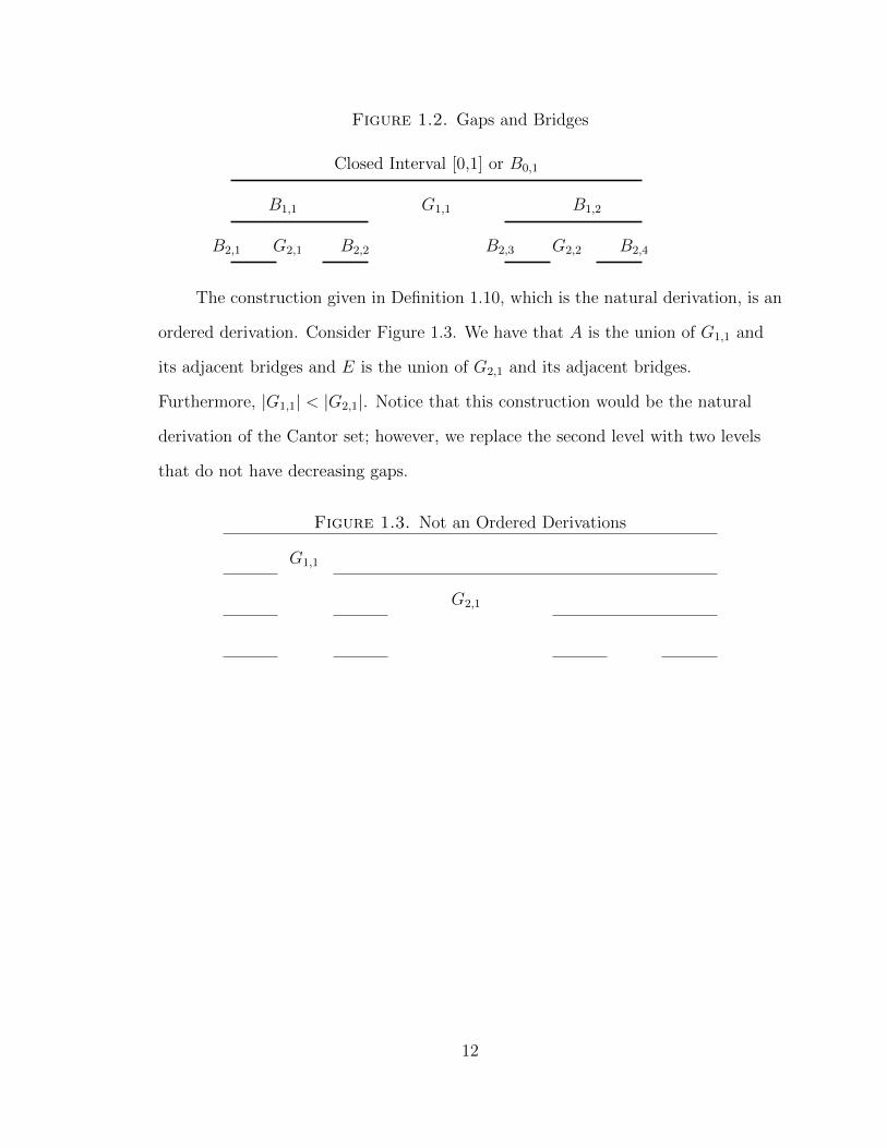
Figure 1.2. Gaps and Bridges

Closed Interval [0,1] or B0,1

B1,1 G1,1 B1,2

B2,1 G2,1 B2,2 B2,3 G2,2 B2,4

The construction given in Definition 1.10, which is the natural derivation, is an

ordered derivation. Consider Figure 1.3. We have that A is the union of G1,1 and

its adjacent bridges and E is the union of G2,1 and its adjacent bridges.

Furthermore, |G1,1| < |G2,1|. Notice that this construction would be the natural

derivation of the Cantor set; however, we replace the second level with two levels

that do not have decreasing gaps.

Figure 1.3. Not an Ordered Derivations

G1,1

G2,1

12

Chapter 2

Properties of Bridges and Gaps

In this chapter, we discuss various properties of the generated Cantor sets.

Gap and bridge length are particularly important for examining the thickness of the

Cantor sets in Chapter 3. One of the main tools used in examining these properties

is the Generalized Mean Value Theorem [7] also known as the Cauchy Mean Value

Theorem.

Theorem 2.1 (Generalized Mean-Value Theorem(GMVT)). Suppose f(x)

and g(x) are continuous on the closed interval [α, β] and differentiable on (α, β),

and assume that g′(x) 6= 0 for all x ∈ (α, β). Then there exists c ∈ (α, β) such that

f(β)− f(α)

g(β)− g(α)=f ′(c)

g′(c).

Before we analyze the components of the generated Cantor sets, we must

understand the construction.

Consider the set of real numbers representable as a continued radical

√m1,m2, . . . such that mi ∈ {a, b}, a, b ∈ N, and a < b. The elements of this set are

called representable. Then the smallest number representable is√a, a, . . . = φa and

the largest is√b, b, . . . = φb. This result follows directly from Proposition 1.9.

Thus, we have that the numbers representable are in the closed interval [φa, φb].

This result is mentioned by Johnson and Richmond [15].

Now, if we consider the representable numbers whose first term is a, we notice

that the largest is√a, b, b, . . . =

√a+ φb. Analogously, we have that the smallest

representable number whose first term is b is√b, a, a, . . . =

√b+ φa. Furthermore,

Johnson and Richmond [15] tell us that for a, b ∈ N and a < b, then√a+ φb <

√b+ φa. Thus, we have a jump between the largest representable

13

number with first term a and the smallest representable number with first term b.

This produces a gap in [φa, φb]. If we remove this gap, we obtain two bridges,

namely, [φ1,√a+ φb] and [

√b+ φa, φb].

Now, if we fix the first term, we have that the second term may be a or b.

Therefore, we can calculate the largest and smallest representable number similar to

the above construction. This will leave us with two addition gaps, one for the case

that the second term is a and another for the case that the second term is b. We

can inductively continue this process.

Suppose we fix the first n terms of the continued radical. That is, we fix the

values of −→w = 〈m1,m2, . . . ,mn〉 such that mi ∈ {a, b}. We have that −→w has length

n and leads to the gap on level n+ 1. When discussing gaps and bridges on level

n+ 1, we refer to −→w as the direction vector. The sequence of a’s and b’s in −→w

determine the left endpoint of a bridge on level n. Notice that since a < b, when

reading the coordinates of −→w , we move to the left bridge on the level below for each

a and the right bridge for each b. Thus we have that −→w directs us to the left

endpoint of a bridge on level n. Furthermore, the jump from a to b in coordinate

n+ 1 will produce a gap on level n+ 1 in the bridge on level n whose left endpoint

was determined by −→w . Thus, all the gaps and bridges on level n+ 1 are determined

by all possible choices of direction vectors −→w of length n.

We begin by considering a gap and its two adjacent bridges. Proposition 2.2

shows that the left bridge is larger than the right bridge.

Proposition 2.2. Given a gap, Gn,k and two adjacent bridges, Bn,i and

Bn,i+1, we have that | Bn,i |>| Bn,i+1 |.

Proof. Suppose that −→w =√w1, w2, . . . , wn navigates us to a certain level on a

generated Cantor set. Then | Bn,i |=√−→w , a+ φb −

√−→w , a+ φa and

14

| Bn,i+1 |=√−→w , b+ φb −

√−→w , b+ φa. We can then define

h(x) =√−→w , x+ φb −

√−→w , x+ φa. Note that | Bn,i |= h(a) and | Bn,i+1 |= h(b).

We now need to consider

h′(x) =1

2k+1(

1√w1, . . . , wk, x+ φb

√w2, . . . , wk, x+ φb · · ·

√wk, x+ φb

√x+ φb

− 1√w1, . . . , wk, x+ φa

√w2, . . . , wk, x+ φa · · ·

√wk, x+ φa

√x+ φa

).

We want to show that h(x) is decreasing, so we can consider each portion of

the denominator separately. We define new functions,

gi(y) =√wi, wi+1, . . . , wk, x+ y. Since the composition of increasing functions is

increasing, each gi(y) is increasing as a function of y.

Therefore, we get that, gi(x+ φb) > gi(x+ φa) > 0. Taking reciprocals, we get

0 <1

gi(x+ φb)<

1

gi(x+ φa). Hence, we get that,

k∏i=1

1

gi(x+ φb)<

k∏i=1

1

gi(x+ φa)

=⇒k∏i=1

1

gi(x+ φb)−

k∏i=1

1

gi(x+ φa)< 0

=⇒ h′(x) =1

2k+1

k∏i=1

1

gi(x+ φb)− 1

2k+1

k∏i=1

1

gi(x+ φa)< 0

Hence, h(x) is decreasing. Ergo, h(a) > h(b) and | Bn,i |>| Bn,i+1 |. �

We consider an analogous idea for gaps. Suppose we choose a bridge Bn,i on

level n of the Cantor set. Then proceeding through the derivation of the Cantor set

to level n+ 2, we have two gaps below Bn,i. Proposition 2.3 compares the lengths of

these two gaps.

Proposition 2.3. Of the two gaps that are 2 levels below any bridge, the

largest gap is on the left.

15

Proof. The length of a gap two levels below the bridge whose left endpoint is

determined by −→w is to be,

h(x) =√−→w , x, b+ φa −

√−→w , x, a+ φb, wherex ∈ {a, b}.

Thenh′(x) =[2n+1

√w1, w2, . . . , wn, x, b+ φa

√w2, . . . , wn, x, b+ φa · · ·

√x, b+ φa

]−1

−[2n+1

√w1, w2, . . . , wn, x, a+ φb

√w2, . . . , wn, x, a+ φb · · ·

√x, a+ φb

]−1

.

We also have that

√b+ φa >

√a+ φb;

thus,1√

b+ φa<

1√a+ φb

.(2.1)

Let A =[2n+1√w1, w2, . . . , wn, x, b+ φa

√w2, . . . , wn, x, b+ φa · · ·

√x, b+ φa

]−1

and B =[2n+1√w1, w2, . . . , wn, x, a+ φb

√w2, . . . , wn, x, a+ φb · · ·

√x, a+ φb

]−1.

Then, each component of B is greater than the corresponding component of A.

Thus, equation (2.1) implies that h′(x) < 0; hence, h is decreasing.

Therefore, of the two gaps that are two levels below any bridge, the largest

gap is on the left. �

Now that we have determined the larger of two bridges below a certain bridge,

we need to consider the largest gap on a given level n. Proposition 2.4 gives this

result.

Proposition 2.4. The largest gap on a given level n is the left-most gap Gn,1.

Proof. Note that | Gn,1 |=√a1, . . . , ak, b+ φa −

√a1, . . . , ak, a+ φb, where

a1 = a2 = · · · = ak = a, is the length of the left-most gap and√w1, . . . , wk, b+ φa −

√w1, . . . , wk, a+ φb represents the length of Gn,i for

1 < i ∈ N (i.e. a gap to the right of Gn,1). We define f(x) =√a1, a2, . . . , ak, x and

16

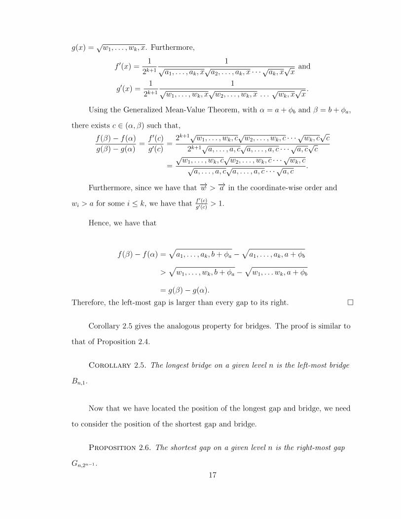
g(x) =√w1, . . . , wk, x. Furthermore,

f ′(x) =1

2k+1

1√a1, . . . , ak, x

√a2, . . . , ak, x · · ·

√ak, x√x

and

g′(x) =1

2k+1

1√w1, . . . , wk, x

√w2, . . . , wk, x . . .

√wk, x

√x.

Using the Generalized Mean-Value Theorem, with α = a+ φb and β = b+ φa,

there exists c ∈ (α, β) such that,

f(β)− f(α)

g(β)− g(α)=f ′(c)

g′(c)=

2k+1√w1, . . . , wk, c√w2, . . . , wk, c · · ·

√wk, c√c

2k+1√a, . . . , a, c

√a, . . . , a, c · · · √a, c

√c

=

√w1, . . . , wk, c

√w2, . . . , wk, c · · ·

√wk, c√

a, . . . , a, c√a, . . . , a, c · · · √a, c

.

Furthermore, since we have that −→w > −→a in the coordinate-wise order and

wi > a for some i ≤ k, we have that f ′(c)g′(c)

> 1.

Hence, we have that

f(β)− f(α) =√a1, . . . , ak, b+ φa −

√a1, . . . , ak, a+ φb

>√w1, . . . , wk, b+ φa −

√w1, . . . wk, a+ φb

= g(β)− g(α).

Therefore, the left-most gap is larger than every gap to its right. �

Corollary 2.5 gives the analogous property for bridges. The proof is similar to

that of Proposition 2.4.

Corollary 2.5. The longest bridge on a given level n is the left-most bridge

Bn,1.

Now that we have located the position of the longest gap and bridge, we need

to consider the position of the shortest gap and bridge.

Proposition 2.6. The shortest gap on a given level n is the right-most gap

Gn,2n−1.

17

Proof. Note that | Gn,2n−1 |=√b1, . . . , bk, b+ φa −

√b1, . . . , bk, a+ φb, where

b1 = b2 = · · · = bk = b, is the length of the right-most gap and√w1, . . . , wk, b+ φa −

√w1, . . . , wk, a+ φb represents the length of Gn,m where

2n−1 > m ∈ N (i.e. a gap to the left of Gn,2n−1). We define f(x) =√b1, b2, . . . , bk, x

and g(x) =√w1, . . . , wk, x. Furthermore,

f ′(x) =1

2k+1

1√b1, . . . , bk, x

√b2, . . . , bk, x · · ·

√bk, x√x

and

g′(x) =1

2k+1

1√w1, . . . , wk, x

√w2, . . . , wk, x . . .

√wk, x

√x

.

Using the Generalized Mean-Value Theorem, with α = a+ φb and β = b+ φa,

there exists c ∈ (α, β) such that

f(β)− f(α)

g(β)− g(α)=f ′(c)

g′(c)=

2k+1√w1, . . . , wk, c√w2, . . . , wk, c · · ·

√wk, c√c

2k+1√b1, . . . , bk, c

√b2, · · · , bk, c · · ·

√bk, c√c

=

√w1, · · · , wk, c

√w2, · · · , wk, c · · ·

√wk, c√

b1, . . . , bk, c√b2, . . . , bk, c · · ·

√bk, c

.

Furthermore, since we have that −→w <−→b , in the coordinate-wise order, and

wi < b for some i ≤ k, we have that f ′(c)g′(c)

< 1.

Hence, we have that

f(β)− f(α) =√b1, . . . , bk, b+ φa −

√b1, . . . , bk, a+ φb

<√w1, . . . , wk, b, φa −

√w1, . . . , wk, a, φb

= g(β)− g(α).

Therefore, the right-most gap is smaller than every gap to its left. �

Example 2.8 below illustrates this fact on level 4 of the Cantor set generated

by continued radicals whose entries are from {1, 2}.

Corollary 2.7. The shortest bridge on a given level n is the right-most

bridge Bn,2n.

18

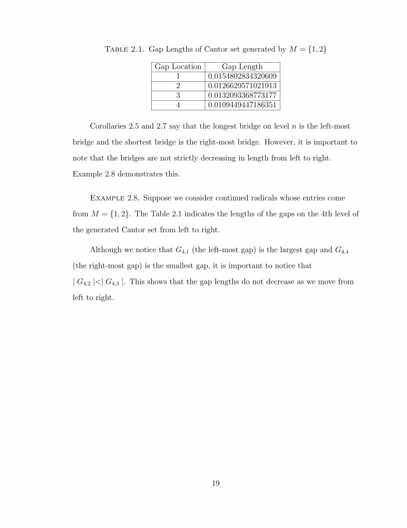
Table 2.1. Gap Lengths of Cantor set generated by M = {1, 2}

Gap Location Gap Length1 0.01548028343206092 0.01266295710219133 0.01320933687731774 0.0109449447186351

Corollaries 2.5 and 2.7 say that the longest bridge on level n is the left-most

bridge and the shortest bridge is the right-most bridge. However, it is important to

note that the bridges are not strictly decreasing in length from left to right.

Example 2.8 demonstrates this.

Example 2.8. Suppose we consider continued radicals whose entries come

from M = {1, 2}. The Table 2.1 indicates the lengths of the gaps on the 4th level of

the generated Cantor set from left to right.

Although we notice that G4,1 (the left-most gap) is the largest gap and G4,4

(the right-most gap) is the smallest gap, it is important to notice that

| G4,2 |<| G4,3 |. This shows that the gap lengths do not decrease as we move from

left to right.

19

Chapter 3

Thickness

In this chapter, we discuss the thickness of Cantor sets. Newhouse [18] defined

the thickness of a Cantor set to be a nonnegative quantity that gives conditions on

when two Cantor sets intersect. Astels [6] gives the following definition.

Definition 3.1. We define the thickness of a level n to be,

τ(n) = infw

(min(| Bn,i |, | Bn,i+1 |)

| Gn,k |

),

where w ranges through all location vectors of a fixed length determined by the level

n and Bn,i and Bn,i+1 are adjacent to Gn,k.

Definition 3.1 only gives us the thickness of a certain level of the Cantor set.

However, we also need to consider the thickness over the entire (ordered) derivation.

Similarly, we have the following definition.

Definition 3.2. We define the thickness of a derivation D to be,

τ(D) = infw

(min(| Bn,i |, | Bn,i+1 |)

| Gn,k |

),

where w is a direction vector of any length and Bn,i and Bn,i+1 are adjacent to Gn,k.

Astels [4], [6] gives information regarding the thickness of Cantor sets

generated by continued fractions. Here, we consider the analogous construction for

continued radicals.

Proposition 3.3. τ(n) is formed by the left-most gap and the right bridge

adjacent to the gap.

20

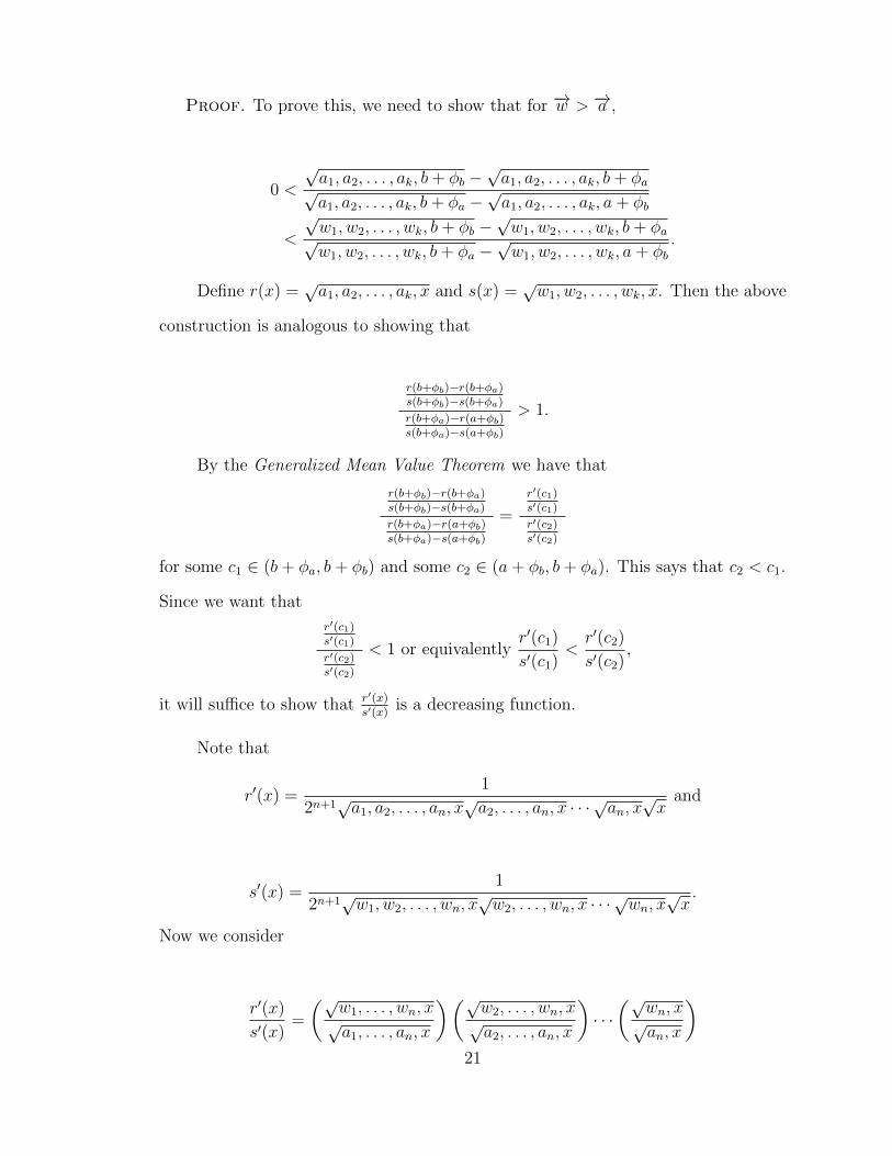
Proof. To prove this, we need to show that for −→w > −→a ,

0 <

√a1, a2, . . . , ak, b+ φb −

√a1, a2, . . . , ak, b+ φa√

a1, a2, . . . , ak, b+ φa −√a1, a2, . . . , ak, a+ φb

<

√w1, w2, . . . , wk, b+ φb −

√w1, w2, . . . , wk, b+ φa√

w1, w2, . . . , wk, b+ φa −√w1, w2, . . . , wk, a+ φb

.

Define r(x) =√a1, a2, . . . , ak, x and s(x) =

√w1, w2, . . . , wk, x. Then the above

construction is analogous to showing that

r(b+φb)−r(b+φa)s(b+φb)−s(b+φa)

r(b+φa)−r(a+φb)s(b+φa)−s(a+φb)

> 1.

By the Generalized Mean Value Theorem we have that

r(b+φb)−r(b+φa)s(b+φb)−s(b+φa)

r(b+φa)−r(a+φb)s(b+φa)−s(a+φb)

=

r′(c1)s′(c1)

r′(c2)s′(c2)

for some c1 ∈ (b+ φa, b+ φb) and some c2 ∈ (a+ φb, b+ φa). This says that c2 < c1.

Since we want that

r′(c1)s′(c1)

r′(c2)s′(c2)

< 1 or equivalentlyr′(c1)

s′(c1)<r′(c2)

s′(c2),

it will suffice to show that r′(x)s′(x)

is a decreasing function.

Note that

r′(x) =1

2n+1√a1, a2, . . . , an, x

√a2, . . . , an, x · · ·

√an, x√x

and

s′(x) =1

2n+1√w1, w2, . . . , wn, x

√w2, . . . , wn, x · · ·

√wn, x

√x.

Now we consider

r′(x)

s′(x)=

(√w1, . . . , wn, x√a1, . . . , an, x

)(√w2, . . . , wn, x√a2, . . . , an, x

)· · ·(√

wn, x√an, x

)21

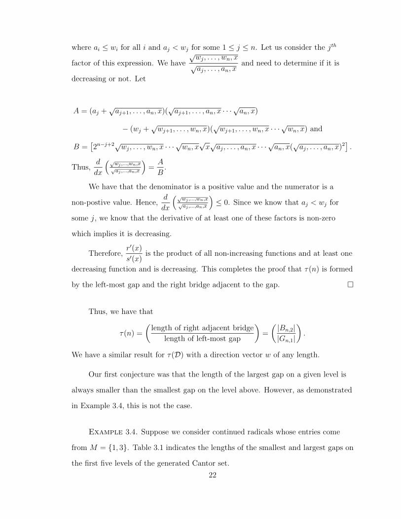
where ai ≤ wi for all i and aj < wj for some 1 ≤ j ≤ n. Let us consider the jth

factor of this expression. We have

√wj, . . . , wn, x√aj, . . . , an, x

and need to determine if it is

decreasing or not. Let

A = (aj +√aj+1, . . . , an, x)(

√aj+1, . . . , an, x · · ·

√an, x)

− (wj +√wj+1, . . . , wn, x)(

√wj+1, . . . , wn, x · · ·

√wn, x) and

B =[2n−j+2√wj, . . . , wn, x · · ·

√wn, x

√x√aj, . . . , an, x · · ·

√an, x(

√aj, . . . , an, x)2

].

Thus,d

dx

(√wj ,...,wn,x√aj ,...,an,x

)=A

B.

We have that the denominator is a positive value and the numerator is a

non-postive value. Hence,d

dx

(√wj ,...,wn,x√aj ,...,an,x

)≤ 0. Since we know that aj < wj for

some j, we know that the derivative of at least one of these factors is non-zero

which implies it is decreasing.

Therefore,r′(x)

s′(x)is the product of all non-increasing functions and at least one

decreasing function and is decreasing. This completes the proof that τ(n) is formed

by the left-most gap and the right bridge adjacent to the gap. �

Thus, we have that

τ(n) =

(length of right adjacent bridge

length of left-most gap

)=

(|Bn,2||Gn,1|

).

We have a similar result for τ(D) with a direction vector w of any length.

Our first conjecture was that the length of the largest gap on a given level is

always smaller than the smallest gap on the level above. However, as demonstrated

in Example 3.4, this is not the case.

Example 3.4. Suppose we consider continued radicals whose entries come

from M = {1, 3}. Table 3.1 indicates the lengths of the smallest and largest gaps on

the first five levels of the generated Cantor set.

22

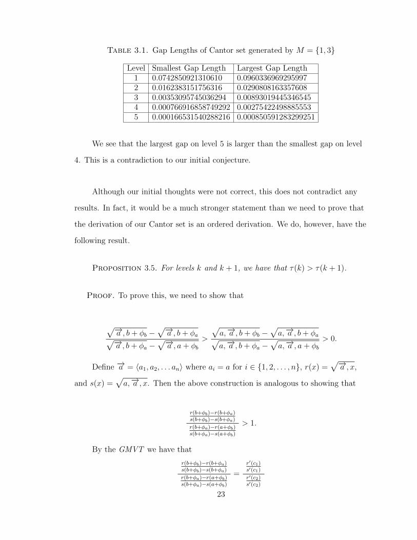
Table 3.1. Gap Lengths of Cantor set generated by M = {1, 3}

Level Smallest Gap Length Largest Gap Length1 0.0742850921310610 0.09603369692959972 0.0162383151756316 0.02908081633576083 0.00353095745036294 0.008930194453465454 0.000766916858749292 0.002754224988855535 0.000166531540288216 0.000850591283299251

We see that the largest gap on level 5 is larger than the smallest gap on level

4. This is a contradiction to our initial conjecture.

Although our initial thoughts were not correct, this does not contradict any

results. In fact, it would be a much stronger statement than we need to prove that

the derivation of our Cantor set is an ordered derivation. We do, however, have the

following result.

Proposition 3.5. For levels k and k + 1, we have that τ(k) > τ(k + 1).

Proof. To prove this, we need to show that

√−→a , b+ φb −√−→a , b+ φa√−→a , b+ φa −√−→a , a+ φb

>

√a,−→a , b+ φb −

√a,−→a , b+ φa√

a,−→a , b+ φa −√a,−→a , a+ φb

> 0.

Define −→a = 〈a1, a2, . . . an〉 where ai = a for i ∈ {1, 2, . . . , n}, r(x) =√−→a , x,

and s(x) =√a,−→a , x. Then the above construction is analogous to showing that

r(b+φb)−r(b+φa)s(b+φb)−s(b+φa)

r(b+φa)−r(a+φb)s(b+φa)−s(a+φb)

> 1.

By the GMVT we have that

r(b+φb)−r(b+φa)s(b+φb)−s(b+φa)

r(b+φa)−r(a+φb)s(b+φa)−s(a+φb)

=

r′(c1)s′(c1)

r′(c2)s′(c2)

23

for some c1 ∈ (b+ φa, b+ φb) and some c2 ∈ (a+ φb, b+ φa). This says that c2 < c1.

Since we want that

r′(c1)s′(c1)

r′(c2)s′(c2)

> 1 or equivalentlyr′(c1)

s′(c1)>r′(c2)

s′(c2),

it will suffice to show that r′(x)s′(x)

is an increasing function.

Note that

r′(x) =1

2n+1√a1, a2, . . . , an, x

√a2, . . . , an, x · · ·

√an, x√x

and

s′(x) =1

2n+2√a1, a2, . . . , an, an+1, x√a2, . . . , an, an+1, x · · ·

√an, an+1, x

√an+1, x

√x.

Now we consider

r′(x)

s′(x)= 2

(√a1, . . . , an, an+1, x√a1, . . . , an, x

)(√a2, . . . , an, an+1, x√a2, . . . , an, x

)· · ·(√

an, an+1, x√an, x

)(√an+1, x) .

Simplifying this, we getr′(x)

s′(x)= 2√a1, a2, . . . , an, an+1, x. This is an increasing

function in x.

Thus, the thickness on a given level is larger than the thickness on all levels

below. �

We calculate the thickness of the middle-thirds Cantor set and the middle-p%

Cantor set in Propositions 3.6 and 3.7, respectively.

Proposition 3.6. The thickness of the middle-third Cantor set (C3) is 1.

Proof. To construct the middle-third Cantor set, we begin with the closed

interval [0, 1]. We first remove the open interval (13, 2

3) which is the middle third of

[0, 1]. From here we have two bridges and a gap. We remove the middle third from

24

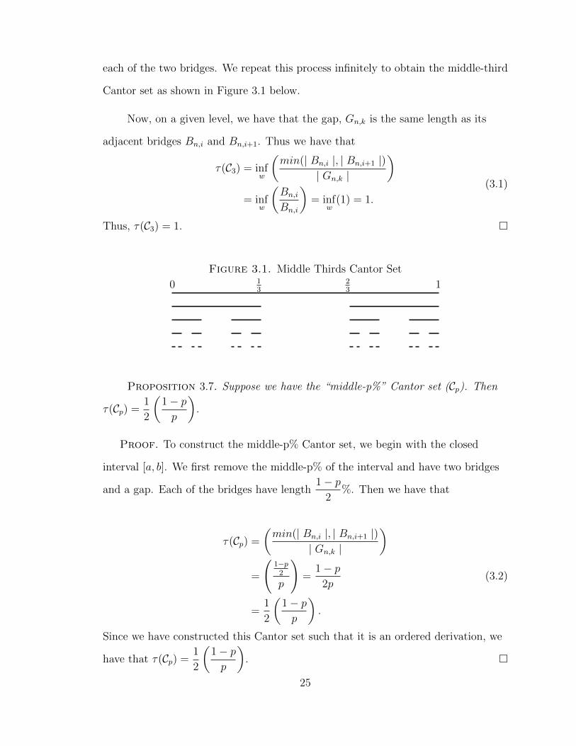
each of the two bridges. We repeat this process infinitely to obtain the middle-third

Cantor set as shown in Figure 3.1 below.

Now, on a given level, we have that the gap, Gn,k is the same length as its

adjacent bridges Bn,i and Bn,i+1. Thus we have that

τ(C3) = infw

(min(| Bn,i |, | Bn,i+1 |)

| Gn,k |

)= inf

w

(Bn,i

Bn,i

)= inf

w(1) = 1.

(3.1)

Thus, τ(C3) = 1. �

Figure 3.1. Middle Thirds Cantor Set

0 13

23

1

Proposition 3.7. Suppose we have the “middle-p%” Cantor set (Cp). Then

τ(Cp) =1

2

(1− pp

).

Proof. To construct the middle-p% Cantor set, we begin with the closed

interval [a, b]. We first remove the middle-p% of the interval and have two bridges

and a gap. Each of the bridges have length1− p

2%. Then we have that

τ(Cp) =

(min(| Bn,i |, | Bn,i+1 |)

| Gn,k |

)=

(1−p

2

p

)=

1− p2p

=1

2

(1− pp

).

(3.2)

Since we have constructed this Cantor set such that it is an ordered derivation, we

have that τ(Cp) =1

2

(1− pp

). �

25

Notice that for p > 13, we have τ < 1 and p < 1

3gives τ > 1.

By Proposition 3.5, we have that the thicknesses of the levels are monotone

decreasing. Furthermore, by Definition 3.2 we have that the thickness of the Cantor

set generated by continued radicals composed from {a, b} is

τ(a, b) = limn→∞

√−→a , b+ φb −√−→a , b+ φa√−→a , b+ φa −√−→a , a+ φb

.

Note that for continued fractions, there is a closed form solution to the values

of thickness of Cantor sets generated by continued fractions composed from {a, b}.

These calculations involve utilizing common recurrence relations for continued

radicals as noted by Astels [5].

We have tried several methods to compute this for the analogous case using

continued radicals; however, we have not been able to find an appropriate approach.

We cannot use the generalized mean value theorem because we have components of

three types in the thickness equation rather than just two types (i.e., we have

b+ φb, b+ φa, and a+ φb).

Notice that as n→∞, the numerator and denominator are both approaching

φa − φa = 0. Thus, we have an indeterminate form and can try applying L’Hopital’s

Rule. We note that the limit is dependent upon n; hence, we need to consider the

discrete analogue of L’Hopital’s Rule. This, however, ends in a more complicated

expression than the original formula.

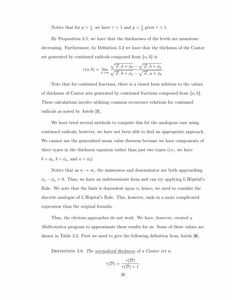
Thus, the obvious approaches do not work. We have, however, created a

Mathematica program to approximate these results for us. Some of these values are

shown in Table 3.2. First we need to give the following definition from Astels [6].

Definition 3.8. The normalized thickness of a Cantor set is

γ(D) =τ(D)

τ(D) + 1.

26

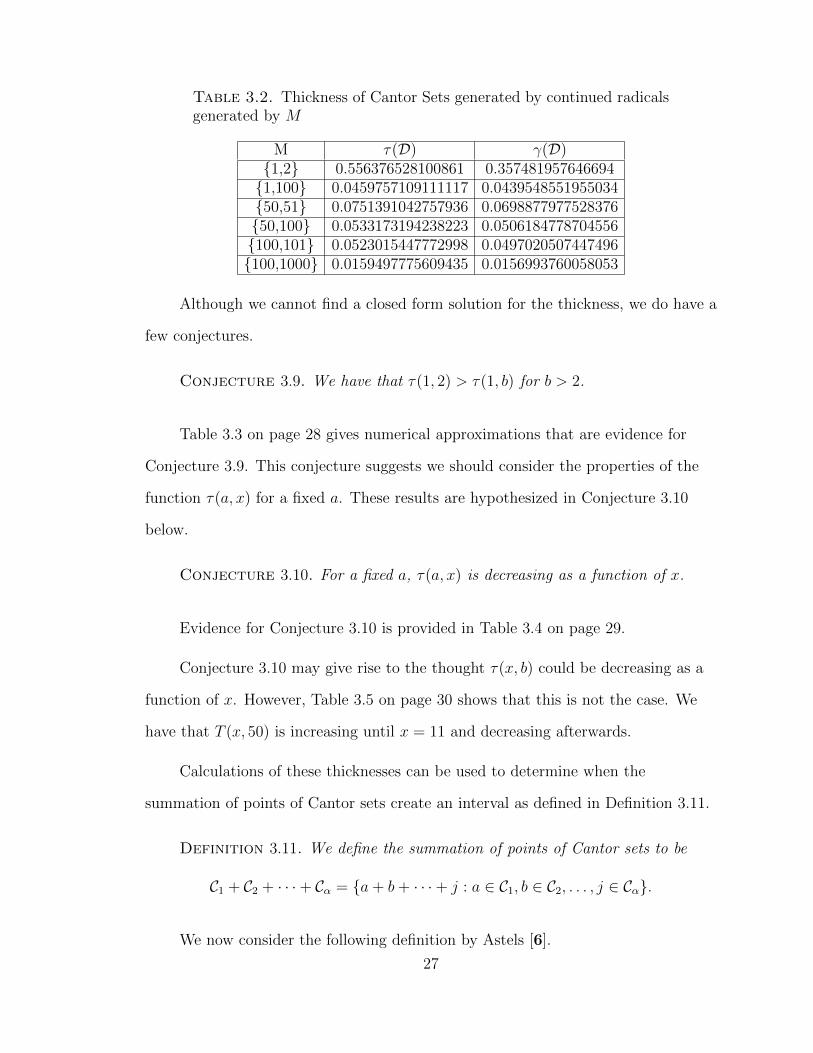
Table 3.2. Thickness of Cantor Sets generated by continued radicalsgenerated by M

M τ(D) γ(D){1,2} 0.556376528100861 0.357481957646694{1,100} 0.0459757109111117 0.0439548551955034{50,51} 0.0751391042757936 0.0698877977528376{50,100} 0.0533173194238223 0.0506184778704556{100,101} 0.0523015447772998 0.0497020507447496{100,1000} 0.0159497775609435 0.0156993760058053

Although we cannot find a closed form solution for the thickness, we do have a

few conjectures.

Conjecture 3.9. We have that τ(1, 2) > τ(1, b) for b > 2.

Table 3.3 on page 28 gives numerical approximations that are evidence for

Conjecture 3.9. This conjecture suggests we should consider the properties of the

function τ(a, x) for a fixed a. These results are hypothesized in Conjecture 3.10

below.

Conjecture 3.10. For a fixed a, τ(a, x) is decreasing as a function of x.

Evidence for Conjecture 3.10 is provided in Table 3.4 on page 29.

Conjecture 3.10 may give rise to the thought τ(x, b) could be decreasing as a

function of x. However, Table 3.5 on page 30 shows that this is not the case. We

have that T (x, 50) is increasing until x = 11 and decreasing afterwards.

Calculations of these thicknesses can be used to determine when the

summation of points of Cantor sets create an interval as defined in Definition 3.11.

Definition 3.11. We define the summation of points of Cantor sets to be

C1 + C2 + · · ·+ Cα = {a+ b+ · · ·+ j : a ∈ C1, b ∈ C2, . . . , j ∈ Cα}.

We now consider the following definition by Astels [6].

27

Table 3.3. Thickness of Cantor sets generated by continued radicalscomposed from {1, b}

b τ(D) γ(D)2 0.556376528100861 0.3574819576466943 0.437824182513184 0.3045046729899254 0.367002837961805 0.2684726232968215 0.319183276235179 0.2419552172811786 0.284382621892108 0.2214158125817417 0.257737462417361 0.2049215119361978 0.236573198321508 0.1913135418450179 0.219287896775729 0.17984915404771210 0.204859058883445 0.17002740475993111 0.192601000815585 0.16149659499184712 0.182035388923834 0.15400164041583013 0.172817577278206 0.14735247887337214 0.164692458768075 0.14140424584037815 0.157466841086656 0.13604436472566516 0.150991524167825 0.13118387146855217 0.145149306072251 0.12675142472914618 0.139846738350957 0.12268907182493419 0.135008324546636 0.11894919325861620 0.130572352758641 0.11549225703250221 0.126487846651723 0.11228514096062822 0.122712297883725 0.10929986080586623 0.119209954632136 0.10651259322592324 0.115950512495125 0.10390291612114025 0.112908100950810 0.101453211504479

Definition 3.12. Let Cj be the Cantor set generated by continued radicals

from {j1, j2}. Then Ij is the interval [φj1 , φj2 ]. We say a sequence of intervals

(I1, . . . , Ik) is compatible if |Ir+1| ≥ |Gj1,1| and |I1|+ · · ·+ |Ir| ≥ |Gr+1

1,1 | for

r = 1, . . . , k − 1 and j = 1, . . . , r where Gj1,1 is gap G1,1 of Cj.

We note that in Astels’ definition, he considers the gap of maximal size in Cj;

however, in our case, gap Gj1,1 is the gap of maximal size.

Theorem 3.13 by Astels [6] tells when the summation of points of a Cantor set

create an interval.

28

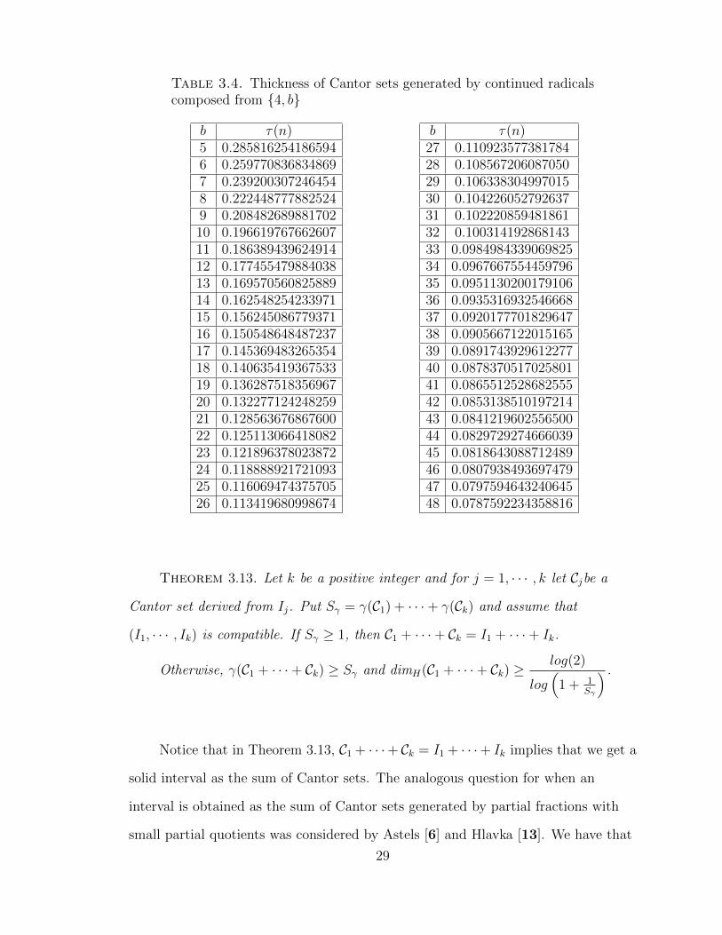
Table 3.4. Thickness of Cantor sets generated by continued radicalscomposed from {4, b}

b τ(n)5 0.2858162541865946 0.2597708368348697 0.2392003072464548 0.2224487778825249 0.20848268988170210 0.19661976766260711 0.18638943962491412 0.17745547988403813 0.16957056082588914 0.16254825423397115 0.15624508677937116 0.15054864848723717 0.14536948326535418 0.14063541936753319 0.13628751835696720 0.13227712424825921 0.12856367686760022 0.12511306641808223 0.12189637802387224 0.11888892172109325 0.11606947437570526 0.113419680998674

b τ(n)27 0.11092357738178428 0.10856720608705029 0.10633830499701530 0.10422605279263731 0.10222085948186132 0.10031419286814333 0.098498433906982534 0.096766755445979635 0.095113020017910636 0.093531693254666837 0.092017770182964738 0.090566712201516539 0.089174392961227740 0.087837051702580141 0.086551252868255542 0.085313851019721443 0.084121960255650044 0.082972927466603945 0.081864308871248946 0.080793849369747947 0.079759464324064548 0.0787592234358816

Theorem 3.13. Let k be a positive integer and for j = 1, · · · , k let Cjbe a

Cantor set derived from Ij. Put Sγ = γ(C1) + · · ·+ γ(Ck) and assume that

(I1, · · · , Ik) is compatible. If Sγ ≥ 1, then C1 + · · ·+ Ck = I1 + · · ·+ Ik.

Otherwise, γ(C1 + · · ·+ Ck) ≥ Sγ and dimH(C1 + · · ·+ Ck) ≥log(2)

log(

1 + 1Sγ

) .

Notice that in Theorem 3.13, C1 + · · ·+ Ck = I1 + · · ·+ Ik implies that we get a

solid interval as the sum of Cantor sets. The analogous question for when an

interval is obtained as the sum of Cantor sets generated by partial fractions with

small partial quotients was considered by Astels [6] and Hlavka [13]. We have that

29

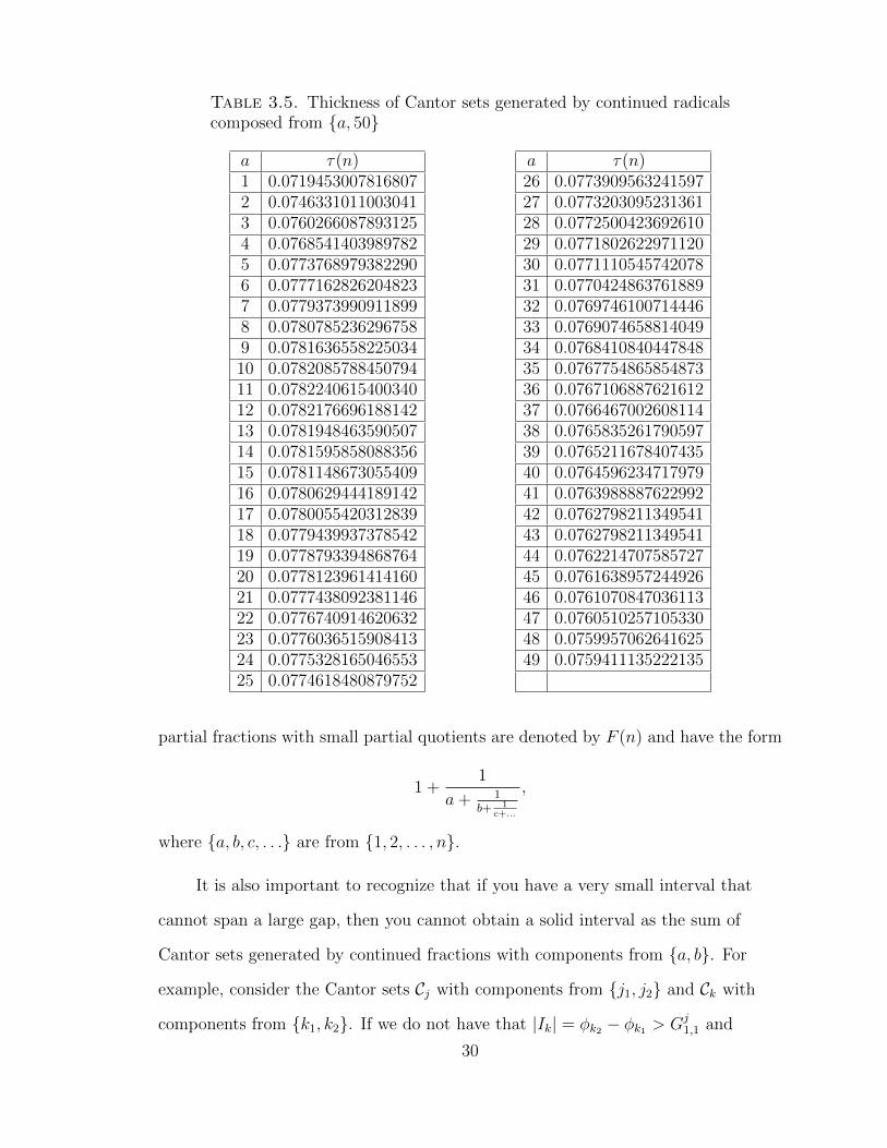
Table 3.5. Thickness of Cantor sets generated by continued radicalscomposed from {a, 50}

a τ(n)1 0.07194530078168072 0.07463310110030413 0.07602660878931254 0.07685414039897825 0.07737689793822906 0.07771628262048237 0.07793739909118998 0.07807852362967589 0.078163655822503410 0.078208578845079411 0.078224061540034012 0.078217669618814213 0.078194846359050714 0.078159585808835615 0.078114867305540916 0.078062944418914217 0.078005542031283918 0.077943993737854219 0.077879339486876420 0.077812396141416021 0.077743809238114622 0.077674091462063223 0.077603651590841324 0.077532816504655325 0.0774618480879752

a τ(n)26 0.077390956324159727 0.077320309523136128 0.077250042369261029 0.077180262297112030 0.077111054574207831 0.077042486376188932 0.076974610071444633 0.076907465881404934 0.076841084044784835 0.076775486585487336 0.076710688762161237 0.076646700260811438 0.076583526179059739 0.076521167840743540 0.076459623471797941 0.076398888762299242 0.076279821134954143 0.076279821134954144 0.076221470758572745 0.076163895724492646 0.076107084703611347 0.076051025710533048 0.075995706264162549 0.0759411135222135

partial fractions with small partial quotients are denoted by F (n) and have the form

1 +1

a+ 1b+ 1

c+...

,

where {a, b, c, . . .} are from {1, 2, . . . , n}.

It is also important to recognize that if you have a very small interval that

cannot span a large gap, then you cannot obtain a solid interval as the sum of

Cantor sets generated by continued fractions with components from {a, b}. For

example, consider the Cantor sets Cj with components from {j1, j2} and Ck with

components from {k1, k2}. If we do not have that |Ik| = φk2 − φk1 > Gj1,1 and

30

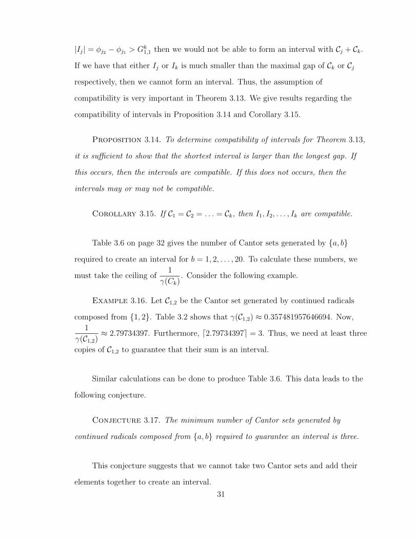
|Ij| = φj2 − φj1 > Gk1,1 then we would not be able to form an interval with Cj + Ck.

If we have that either Ij or Ik is much smaller than the maximal gap of Ck or Cj

respectively, then we cannot form an interval. Thus, the assumption of

compatibility is very important in Theorem 3.13. We give results regarding the

compatibility of intervals in Proposition 3.14 and Corollary 3.15.

Proposition 3.14. To determine compatibility of intervals for Theorem 3.13,

it is sufficient to show that the shortest interval is larger than the longest gap. If

this occurs, then the intervals are compatible. If this does not occurs, then the

intervals may or may not be compatible.

Corollary 3.15. If C1 = C2 = . . . = Ck, then I1, I2, . . . , Ik are compatible.

Table 3.6 on page 32 gives the number of Cantor sets generated by {a, b}

required to create an interval for b = 1, 2, . . . , 20. To calculate these numbers, we

must take the ceiling of1

γ(Ck). Consider the following example.

Example 3.16. Let C1,2 be the Cantor set generated by continued radicals

composed from {1, 2}. Table 3.2 shows that γ(C1,2) ≈ 0.357481957646694. Now,

1

γ(C1,2)≈ 2.79734397. Furthermore, d2.79734397e = 3. Thus, we need at least three

copies of C1,2 to guarantee that their sum is an interval.

Similar calculations can be done to produce Table 3.6. This data leads to the

following conjecture.

Conjecture 3.17. The minimum number of Cantor sets generated by

continued radicals composed from {a, b} required to guarantee an interval is three.

This conjecture suggests that we cannot take two Cantor sets and add their

elements together to create an interval.

31

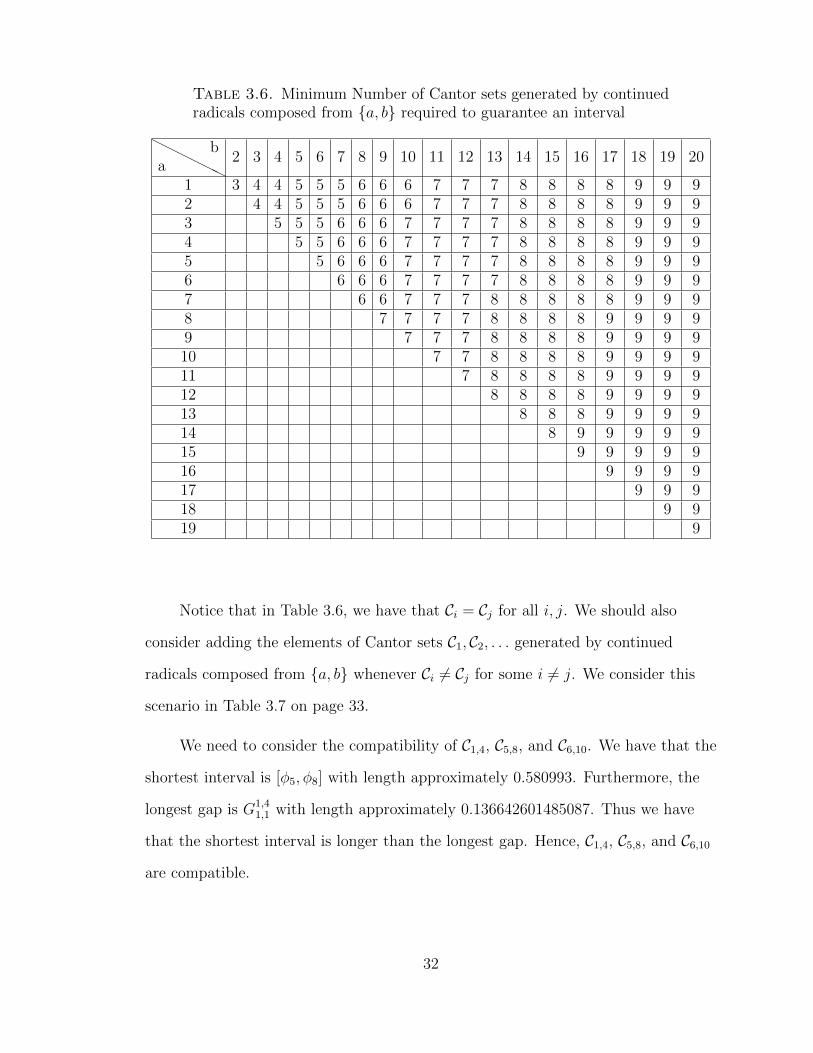
Table 3.6. Minimum Number of Cantor sets generated by continuedradicals composed from {a, b} required to guarantee an interval

HHHH

HHab

2 3 4 5 6 7 8 9 10 11 12 13 14 15 16 17 18 19 20

1 3 4 4 5 5 5 6 6 6 7 7 7 8 8 8 8 9 9 92 4 4 5 5 5 6 6 6 7 7 7 8 8 8 8 9 9 93 5 5 5 6 6 6 7 7 7 7 8 8 8 8 9 9 94 5 5 6 6 6 7 7 7 7 8 8 8 8 9 9 95 5 6 6 6 7 7 7 7 8 8 8 8 9 9 96 6 6 6 7 7 7 7 8 8 8 8 9 9 97 6 6 7 7 7 8 8 8 8 8 9 9 98 7 7 7 7 8 8 8 8 9 9 9 99 7 7 7 8 8 8 8 9 9 9 910 7 7 8 8 8 8 9 9 9 911 7 8 8 8 8 9 9 9 912 8 8 8 8 9 9 9 913 8 8 8 9 9 9 914 8 9 9 9 9 915 9 9 9 9 916 9 9 9 917 9 9 918 9 919 9

Notice that in Table 3.6, we have that Ci = Cj for all i, j. We should also

consider adding the elements of Cantor sets C1, C2, . . . generated by continued

radicals composed from {a, b} whenever Ci 6= Cj for some i 6= j. We consider this

scenario in Table 3.7 on page 33.

We need to consider the compatibility of C1,4, C5,8, and C6,10. We have that the

shortest interval is [φ5, φ8] with length approximately 0.580993. Furthermore, the

longest gap is G1,41,1 with length approximately 0.136642601485087. Thus we have

that the shortest interval is longer than the longest gap. Hence, C1,4, C5,8, and C6,10

are compatible.

32

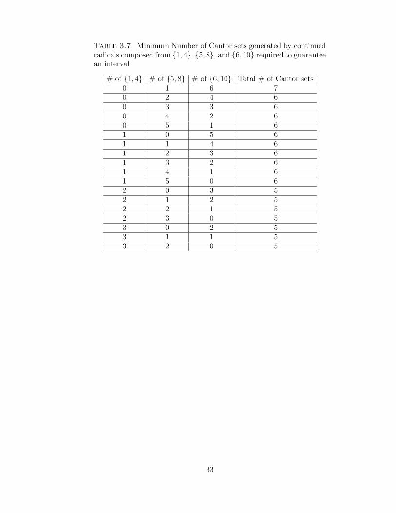
Table 3.7. Minimum Number of Cantor sets generated by continuedradicals composed from {1, 4}, {5, 8}, and {6, 10} required to guaranteean interval

# of {1, 4} # of {5, 8} # of {6, 10} Total # of Cantor sets0 1 6 70 2 4 60 3 3 60 4 2 60 5 1 61 0 5 61 1 4 61 2 3 61 3 2 61 4 1 61 5 0 62 0 3 52 1 2 52 2 1 52 3 0 53 0 2 53 1 1 53 2 0 5

33

Chapter 4

Measure

Generally, the Cantor set is thought to have measure zero. In this chapter we

examine the measure of the middle-thirds Cantor set, the ε-Cantor set, and the

Cantor sets generated by continued radicals generated by the set {a, b}.

Proposition 4.1. The middle-thirds Cantor set, C3 has measure zero.

Proof. Recall the notation from Chapter 1. We have that I contains no gaps

(i.e. removed intervals), C0 contains 1 = 20 gap, C1 ∪ Cc0 contains 2 = 21 gaps, . . .

Cm

[m−1⋃i=0

Cci

]contains 2m gaps, . . .. Therefore, we have that on Cm, we remove 2m

intervals. Furthermore, we see that the length of the gaps removed will be 0, 13, 1

32,

133, . . . for I, C0, C1, C2, . . ., respectively. Furthermore, we have that µ([0, 1] \ C) is

the sum of the lengths of the gaps; thus, we have

µ([0, 1] \ C) =20

31+

21

32+

22

33+ . . .

=∞∑m=0

(2m

3m+1

)

=

(1

3

) ∞∑m=0

(2

3

)m=

(1

3

)1

1− 23

=

(1

3

)(3) = 1

Thus we have that µ([0, 1] \ C3) = 1 = µ([0, 1])− µ(C3) = 1− µ(C3). Thus,

µ(C3) = 0. �

It is important to note that the measure of Cantor sets is not always zero.

Aliprantis and Burkinshaw [1] give an example of such a set.

34

Example 4.2 (The ε-Cantor set). To construct the ε-Cantor set, Cε, we begin

with 0 < ε < 1 and let δ = 1− ε. We begin with the closed interval [0, 1] = A0.

From the center of this interval, we remove an open interval with length δ2. Thus we

have that A1 = [0, (12− δ

4)] ∪ [(1

2+ δ

4), 1]. Then µ(A1) = 1− δ

2.

Now, from the center of each of the two disjoint closed intervals of A1, we

remove an open interval of length δ23

. The union of these four disjoint closed sets is

A2. Then we have µ(A2) = 1− [µ(A1)− ( δ8

+ δ8)] = 1− (1

2+ 1

4)δ = 1− 3δ

4.

We have that An is the disjoint union of 2n closed intervals of the same length

that satisfy µ(An) = 1− (12

+ . . .+ 12n

+ 12n+1 )δ. From the center of each of the 2n

disjoint closed intervals of An, we remove an open interval of length δ22n+1 . Then we

have that An+1 is the union of these 2n+1 closed intervals. Thus we have that

µ(An+1) = 1− (12

+ . . .+ 12n

+ 12n+1 )δ.

We then have that Cε =∞⋂n=1

An. Furthermore,

µ(Cε) = limµ(An) = 1−

(∞∑n=1

1

2n

)δ = 1− δ = ε > 0.

To see that the ε-Cantor set is in fact a Cantor set, we need to consider the

following definition given by Cabrelli, Paulaskas, Lithuania, and Shonkwiler [9].

Definition 4.3. A general Cantor set is a compact, perfect, totally

disconnected subset of the real line.

Note that Astels [6] gives a weaker definition of generalized Cantor sets. He

states that a generalized Cantor set is any set C of real numbers of the form

C = I \⋃i≥1

Gi where I is a finite closed interval and {Gi : i ≥ 1} is a countable

collection of disjoint open intervals contained in I. This definition seems to not be

equivalent to Definition 4.3. For our results, we will use the definition by Cabrelli,

Paulaskas, Lithuania, and Shonkwiler [9].

35

Proposition 4.4. The ε-Cantor set, Cε, is a general Cantor set.

Proof. Note that the ε-Cantor set is closed and bounded; thus, by the

Heine-Borel theorem, we have that it is a compact subset of R.

Now, we need to show that Cε is a perfect subset of R. Note that a set A is

said to be perfect if and only if every point in A is a limit point of A, or

equivalently, if no point in A is isolated.

Now, consider the midpoints of the removed intervals on level n. We have that

these are Mn ={m

2n

}where m ∈ {1, 2, . . . , 2n − 1}. Since M =

∞⋃n=1

Mn is a set of

dyadic fractions, we have that M is dense on [0, 1].

Furthermore, between any two midpoints of gaps, we have an interval. By the

construction of Cε, the endpoints of intervals are never removed. Let

x ∈ Cε \ {0, 1} = D and B(x, r) be an open-ball centered at x with radius r. We

can find n such that B(x, r) contains at least two midpoints of gaps. Therefore,

B(x, r) contains at least one interval; hence, it contains at least 2 distinct points

y, z ∈ D. Thus, we have that x is not isolated and since 0 and 1 are limit points,

every point in Cε is a limit point of Cε. Thus, Cε is a perfect subset of R.

Now, since the midpoints of gaps are dense, any alleged interval will have

points removed since midpoints of gaps are removed. Thus, Cε is totally

disconnected.

Therefore, Cε is a compact, perfect, totally disconnected subset of the real line;

thus, it is a general Cantor set. �

The ε-Cantor set demonstrates the necessity of considering the measure of the

Cantor sets generated by continued radicals generated with two values a, b.

Proposition 4.5. The measure of the Cantor sets generated by continued

radicals generated with two values a, b is 0.

36

Proof. Case 1: Suppose a > 1. Then the length of the left bridge is√−→a , φb − φa = |Bn,1|. By Corollary 2.5, we have that the left-most bridge is the

largest on a given level. Thus, each of the 2n bridges on level n are smaller than or

equal to the length of the left-most bridge.

Now2n∑i=1

|Bn,i| < 2n|Bn,1| = 2n(√−→a , φb − φa).

We now need to consider limn→∞

2n(√−→a , φb − φa). We know that

f(x) =√a1, a2, . . . , an, x is a contraction. Thus, by Proposition 1.13, we have that

(√a1, . . . an, φb −

√a1, . . . , an, φa) ≤

1

2n+1√an+1

(φb − φa). Therefore,

limn→∞

2n(√−→a , φb − φa) ≤ lim

n→∞2n(

1

2n+1√an+1

)(φb − φa)

= (φb − φa) limn→∞

(1

2√an+1

)= 0.

(4.1)

Thus, for a > 1, we have that the measure of the generated Cantor set is 0.

Case 2: Suppose a = 1. We have that the length of the bridges on level n is√w1, w2, . . . , wn, 1 + φb −

√w1, w2, . . . wn, 1 + φ1. Furthermore, −→w is a vector of

length n generated by {1, b}. We have that

√w1, w2, . . . , wn, 1 + φb −

√w1, w2, . . . wn, 1 + φ1

<1

2n+1√w1w2 · · ·wn1

(φb − φ1)

=1

2n+1√bk

(φb − φ1) if −→w has exactly k b’s.

Of the 2n bridges, we need to consider how many actually have exactly k

occurrences of b in their −→w . We have that

(n

k

)of these exist. Therefore, the sum

of the lengths of the 2n bridges on level n is less than

n∑k=0

(n

k

)1

2n+1√bk

(φb − φ1) =(φb − φ1)

2

n∑k=0

(n

k

)1

2n1√bk.

37

Here we have thatn∑k=0

(n

k

)1

2n= 1 since the sum of row n of Pascal’s triangle is 2n.

Thus,n∑k=0

(n

k

)1

2n√bk

is a weighted average of 1, 1√b, 1√

b2, . . ., 1√

bn.

Now, let ε > 0 be given. We need to find the smallest j such that 1√bj< ε

2.

This gives us j terms that are greater than ε2, namely 1, 1√

b, 1√

b2, . . . , 1√

bj−1.

Furthermore, the remaining n− j terms are all below ε2. As n→∞, we have that

their weights dominate the summation which makes the weighted average less than

ε for all ε > 0.

Thus, for a = 1, we have that the measure is in fact zero. �

For the case of a = 1, we have an alternate proof as shown below.

Proof 2 of Proposition 4.5. Suppose a = 1. We have that the length of the

bridges on level n is√w1, w2, . . . , wn, 1 + φb −

√w1, w2, . . . wn, 1 + φ1. Furthermore,

−→w is a vector of length n generated by {1, b}. We have that

√w1, w2, . . . , wn, 1 + φb −

√w1, w2, . . . wn, 1 + φ1

<1

2n+1√w1w2 · · ·wn(1)

(φb − φa)

=1

2n+1√bk

(φb − φ1) if −→w has exactly k b’s.

Of the 2n bridges, we need to consider how many actually have exactly k

occurrences of b in their −→w . We have that

(n

k

)of these exist. Therefore, the sum

of the lengths of the 2n bridges on level n is less than

38

n∑k=0

(n

k

)1

2n+1√bk

(φb − φ1)

<

n∑k=0

(n

k

)1

2n√bk

(φb − φ1) for 2 ≤ b ∈ Z

<

2n∑k=0

(2n

n

)1

22n√

2k(φb − φ1) (wlog use 2n).

Romik [21] gives us Stirling’s approximation which states that

n! ∼√

2πn(ne

)n. Thus we have that (2n)! ∼ 2

√πn(

2ne

)2n. Thus, we consider

limn→∞

2n∑k=0

(2n

n

)1

22n√

2k(φb − φ1)

= limn→∞

2n∑k=0

(2n)!

n!21

22n√

2k(φb − φ1)

= limn→∞

2n∑k=0

2√πn(

2ne

)2n

(√

2πn(ne

)n)2

1

22n√

2k(φb − φ1)

= limn→∞

2n∑k=0

1√πn2k

(φb − φ1)

= (φb − φ1) limn→∞

1√πn

2n∑k=0

1√2k

= (φb − φ1)

(limn→∞

1√πn

)(limn→∞

2n∑k=0

1√2k

)= 0.

Note that∞∑k=0

1√2k

converges by the ratio test. Furthermore, limn→∞

1√πn

= 0.

Thus, the measure of the Cantor set generated by continued radicals generated by

{1, b} is zero. �

We note here that there appears to be a relationship between this construction

and the Gamma function. We have the common identity that Γ

(1

2

)=√π and(

2n

n

)=

Γ(2n+ 1)

Γ2(n+ 1).

39

Chapter 5

Conclusion

We have been able to answer several questions regarding the lengths of gaps

and bridges of Cantor sets generated by continued radicals. We have also studied

the measure of these Cantor sets and gotten some results regarding their thickness.

The most important open question is the calculation of the thickness. Being

able to find a closed form solution for the thickness of the Cantor sets generated by

continued radicals would provide a nice result. This would allow us to obtain the

exact thickness without using computational approximations. Since L’Hopital’s

Rule gave us a more complicated expression, there may be a method of doing

L’Hopital’s Rule in reverse to obtain a form that simplifies more easily. However, if

this does not provide any insight, we may be able to use asymptotics to obtain a

sharper approximation.

Even if the thickness cannot be calculated with a closed form solution, we give

further consideration to Conjectures 3.10 and 3.17. Although numerical analysis

provides evidence for these conjectures, there may be some other tools that can be

used to prove them.

Furthermore, we have only considered continued radicals generated by {a, b}

where a, b are natural numbers. This does not consider continued radicals allowing

zeros as their components. It would be interesting to see how allowing zero changes

the results. Some preliminary numerical results indicate that if the thickness is

unchanged, Conjecture 3.17 is false and the minimum number of Cantor sets

required to guarantee an interval is two. However, as noted in the introduction, it

has not been proven that continued radicals generated by {0, b} is homeomorphic to

the Middle-Thirds Cantor set. Therefore, it is necessary to consider this case.

40

This leads to the natural question of considering the use of all integers

(including negative). With this, complex numbers arise creating complications with

our constructions. However, Rhode [20] and Sizer and Wiredu [24] discuss

continued radicals in the complex plane. Furthermore, Leighton and Thron [17]

consider the analogous problem for continued fractions. Perhaps some of these

results can be applied to continued radicals. Additionally, information may be

obtained from the discussion by Wagon [26] regarding complex Cantor sets.

Combining these two areas may produce some results regarding Cantor sets

generated by complex continued radicals.

41

BIBLIOGRAPHY

[1] Aliprantis, C. & Burkinshaw, O. “Principles of Real Analysis (2nd Ed.).” Academic Press:San Diego, CA. 1990.

[2] Allen, E. J. “Continued Radicals.” The Mathematical Gazette, 69 (450), 261-263, 1985.[3] Andrushkiw, R. “On the Convergence of Continued Radicals with Applications to Polynomial

Equations.” J. Franklin Inst., 319 (4), 391-396, 1985.[4] Astels, S. “Cantor Sets and Numbers with Restricted Partial Quotients.” Transactions of the

American Mathematical Society, 352 (1), 133-170, 1999.[5] Astels, S. “Thickness Measures for Cantor Sets.” Electronic Research Announcements of the

American Mathematical Society, 5, 108-111, 1999.[6] Astels, S. “Sums of Numbers with Small Partial Quotients.” Proceedings of the American

Mathematical Society, 130 (3), 637-642, 2001.[7] Bartle, R. G. & Sherbert, D. R. “Introduction to Real Analysis, 4th ed.” John Wiley & Sons

Inc: New York, NY. 2011.[8] Borwein, J. & de Barra, G. “Nested Radicals.” The American Mathematical Monthly, 98 (8),

735-739, 1991.[9] Cabrelli, C., Molter, U., Paulauska, M., & Shonkwiler, R. “Hausdorff Measure of p-Cantor

Sets.” Real Analysis Exchange, 30 (2), 413-434, 2004.[10] Efthimiou, C. J. “A Class of Periodic Continued Radicals.” The American Mathematical

Monthly, 119 (1), 52-58, 2012.[11] Hensley, D. “Continued Fraction Cantor Sets, Hausdorff Dimension, and Functional

Analysis.” Journal of Number Theory, 40, 336-358, 1992.[12] Herschfeld, A. “On Infinite Radicals.” American Mathematical Monthly, 98, 735-739, 1991.[13] Hlavka, J. “Results on Sums of Continued Fractions.” Transactions of the American

Mathematical Society, 211, 123-134, 1978.[14] Hunt, B. R., Kan, I., & Yorke, J. A. “When Cantor Sets Intersect Thickly” Transactions of

the American Mathematical Society, 339 (2), 869-888, 1993.[15] Johnson, J. & Richmond, T. “Continued Radicals.” The Ramanujan Journal, 15 (2), 259-

273, 2008.[16] Laugwitz, D. “Kettenwurzeln und Kettenoperationen.” Elemente der Mathematik, 45 (4),

89-98, 1990.[17] Leighton, W. & Thron, W.J. “Continued Fractions with Complex Elements.” Duke

Mathematical Journal, 9 (4), 763-772, 1942.[18] Newhouse, S. “Nondensity of axiom A(a) on S2.” Proceedings of the Symposia in Pure

Mathematics, American Mathematical Society, 14, 191-202, 1970.[19] Nyblom, M. A. “More Nested Square Roots of 2.” The American Mathematical Monthly, 112

(9), 822-825, 2005.[20] Rhode, H. “Complex Iterated Radicals.” The American Mathematical Monthly, 81 (1), 14-21,

1974.[21] Romik, D. “Stirlings Approximation for n!: the Ultimate Short Proof?.” The American

Mathematical Monthly, 107 (6), 556-557, 2000.[22] Servi, L. D. “Nested Square Roots of 2.” The American Mathematical Monthly, 110 (4),

326-330, 2003.[23] Sizer, W. “Continued Roots.” Mathematics Magazine, 59 (1), 23-27, 1986.[24] Sizer, W. & Wiredu, E. K. “Convergence of Some Continued Roots in the Complex Plane.”

Bull Malaysian Math. Society, 19 (2), 1-7, 1996.[25] Sury, B. “Ramanujan’s Route to Roots of Roots.” Talk in IIT Madras, 2007.[26] Wagon, S. “Mathematica in Action: Problem Solving Through Visualization and

Computation (3rd Ed.).” Springer: New York, NY. 2010.[27] Zimmerman, S. & Ho, C. “On Infinitely Nested Radicals.” Mathematics Magazine, 81 (1),

3-15, 2008.

42