Embed Size (px)
Citation preview

CONTENTS
Borsos, E., Makra, L., Béczi, R., Vitányi, B. and Szentpéteri, M.: Anthropogenic air pollution in the ancient times .................................................................................................5 Bottyán, Z., Balázs, B., Gál, T. and Zboray, Z.: A statistical approach for estimating mean maximum urban temperature excess .........................................................17 Deák, J.Á.: Landscape changes of the Lódri-tó - Kisiván-szék - Subasa area in the Dorozsma-Majsaian Sandlands ............................................................................................27 Gulyás, Á., Unger, J., Balázs, B. and Matzarakis, A.: Analysis of the bioclimatic conditions within different surface structures in a medium-sized city (Szeged, Hungary) ..............................................................................................................................37 Juhos, I., Béczi, R. and Makra, L.: Comparison of artifical intelligence prediction techniques in NO and NO2 concentrations’ forecast................................................................45 Kaszala, R., Bárány-Kevei, I. and Polyák-Földi, K.: Heavy metal content of the vegetation on karstic soils ....................................................................................................57 Kircsi, A. and Szegedi, S.: The development of the urban heat island studied on temperature profiles in Debrecen .........................................................................................63 Kürti, L. and Bárány-Kevei, I.: Landscape evaluation on sodic land of Pély at Hungary (ecotope-forming value) ........................................................................................71 Lakatos, L. and Gulyás, Á.: Connection between phenological phases and urban heat island in Debrecen and Szeged, Hungary .....................................................................79 Makra, L., Mayer, H., Béczi, R. and Borsos, E.: Evaluation of the air quality of Szeged with some assessment methods................................................................................85 Sümeghy, Z. and Unger, J.: Classification of the urban heat island patterns........................93 Sümeghy, Z. and Unger, J.: Seasonal case studies on the urban temperature cross-section ................................................................................................................................101 Szegedi, S. and Kircsi, A.: Effects of the synoptic conditions in the development of the urban heat island in Debrecen, Hungary ........................................................................111 Vitányi, B., Makra, L., Juhász, M., Borsos, E., Béczi, R. and Szentpéteri, M.: Ragweed pollen concentration in the function of meteorological elements in the south-eastern part of Hungary ............................................................................................121 Notes to contributors of Acta Climatologica et Chorologica .............................................131
3

ACTA CLIMATOLOGICA ET CHOROLOGICA Universitatis Szegediensis, Tom. 36-37, 2003, 5-15.
ANTHROPOGENIC AIR POLLUTION IN THE ANCIENT TIMES
E. BORSOS1, L. MAKRA1, R. BÉCZI1, B. VITÁNYI2 and M. SZENTPÉTERI3
1Department of Climatology and Landscape Ecology, University of Szeged, P.O.Box 653, 6701 Szeged, Hungary E-mail: [email protected]
2Bocskai István Secondary and Technical School, Ondi út 1, 3900 Szerencs, Hungary 3Teachers’ Training Institute, Juhász Gyula Teachers’ Training Faculty,
University of Szeged; Hungary
Összefoglalás – Napjainkig számos összefoglaló kötet, illetve tanulmány jelent meg az elmúlt korok környezetszennyezéséről (pl. Brimblecombe, 1987; Brimblecombe and Pfister, 1990; McNeill, 2001, Bowler and Brimblecombe, 2000; Karatzas, 2000, 2001). E dolgozat célja, hogy további adalékokkal szolgáljon a tárgykörben – elsősorban az ókorból és a középkorból. Summary – Several comprehensive publications have been issued recently on the environmental pollution of the past times (e.g. Brimblecombe, 1987; Brimblecombe and Pfister, 1990; McNeill, 2001, Bowler and Brimblecombe, 2000; Karatzas, 2000, 2001). The aim of the study is to give further information on the subject – mainly in the ancient and the medieval times.
Key words: lead mining, copper mining, lead pollution of teeth, lead pollution of the atmosphere, copper pollution of the atmosphere
POLLUTION OF THE ENVIRONMENT IN THE ANCIENT TIMES
Pollution of the environment has started with the appearance of humans. When Homo Sapiens lighted fire, its smoke proved to be the first environmental pollution. Air pollution of inner spaces has started with using fuels for heating and cooking. Walls of caves, inhabited many thousand years ago, are covered by thick layers of soot. Hence, it is supposed that breathing of cavemen was difficult due to the smoke, which also irritated their eyes in the closed room. Lungs of mummified bodies from the Palaeolithic era are frequently black. In the first places, which served for living, smoke was not driven away (one of its practical reasons might have been protection against mosquitoes) and cavemen then lived in smoky rooms (McNeill, 2001). [Millions of people have recently been living in this way. In 1993, when we were in Nepal, we were trekking in the Langtang National Park and visited many little villages and stayed at „hotels”, when going on the southern slopes towards the High Himalayas. Even recently, smoke of fire is not driven away from buildings here. Walls of the houses are built of metamorphic slates, without binder and their roof are covered with rush matting. When lighting fire, there is thick smoke inside the house, irritating the eyes and making difficult breathing. It is impossible to sleep, even one can only stay there for a short time. And from outside, the house seems to be on fire, smoke is streaming out through the slits and gaps of the walls.] One has been living together with this harmful effect of air pollution for many thousand years.
5

Emőke Borsos, László Makra, Rita Béczi, Béla Vitányi and Mária Szentpéteri
Pollution of the environment was responsible for several kinds of illnesses in the early times. The very first pollution of the environment might have been the human excrement. Bowel bacterium living in the human body, such as the Escherichia coli, might have got from faeces to springs, which might have infected the early humans. This environmental pollution has been the reason of millions’ illnesses even recently. In China, where a comprehensive system was developed for waste salvage even in the ancient times, fertilization with faeces was an important element of the agriculture even many thousand years ago. Productivity of the alluvial plain in the eastern part of the country has been maintained in this way for over 4,000 years. In several regions of China this tradition has been followed even recently. Han Suyin took the following note: „In Chengtu (capital of Sechuan Province) those families, who owned the city channel and, in this way, could send the accumulated faeces in countryside, have belonged to the richest ones even in the 20th century (till 1949)” (Markham, 1994). Fertilization of rice-paddies with faeces contributed largely to pollution of ground water which, in this way, is unfit for drinking in the whole tropic Asia. If, on the other hand, water is boiled, then salts are deposited and, in this way, it loses its taste. Flavouring boiled water with tee leaf comes from China and it started to spread in the empire about 2,000 B.C. and then all over Asia (Makra, 2000).
Dust pollution also appeared in the early times. According to the assumption of Janssens, in the New Stone Age in stone mines, e.g. in Obourg, people who carved flint from limestone day by day might have suffered from silicosis. The reason of it was that they breathed stone powder all the day. Sometimes the geographical position of the place considered was the cause of appearance of some diseases. Investigations revealed that near Broken, in the territory of the recent Zambia, Hominides who lived about 200,000 years ago, suffered from lead poisoning. The reason of this illness was that lead oozed from the neighbouring seam into the spring near their cave (Markham, 1994).
Effect of damaging the environment by ancient civilizations caused long-lasting changes in the environment, which can be experienced even recently. These effects appeared on regional scale; however, they did not cause global changes. During the 1,700 years long period between 3,500 B.C. and 1,800 B.C. in the plain of Tiger and Euphrates Rivers, efficiency of the Sumerian agriculture worsened more and more and wheat production decreased gradually, because the soil became salty. Water used for irrigation raises ground water level, and if redundant water is not driven away by channels, then soil is saturated with water, salts loose from soil and are deposited on the surface and then make an unbroken layer. Sumerian noted this process as „the soil surface became white”. Water used for irrigation washed soils totally and made the region more and more unfit for agricultural production. This phenomenon largely contributed to the decline of the Sumerian culture. (Markham, 1994; Mészáros, 2002).
In the ancient times air pollution had substantial consequences only in cities. In the early towns, as in some recent settlements, penetrating stink might have frequently feeled, source of which was tainted meat, rotten foods and excrement. In these settlements, during siege – when there was no possibility to remove materials emitting aggressive smells – unbearable circumstances were developed. Egyptian historical records mention that when Nubian besieging troops cut off Hermopolis – which is situated on the left bank of the Nile, half-way between Theba and Memphis – the inhabitants rather handed over the town and presented a petition for peace than to bear further their own stinking air (Brimblecombe, 1995). In the ancient cities smell pollution was generally important. Aristoteles (384 B.C. – 322 B.C.) mentioned in his work Athenaion Politeia a rule that mature should be placed outside the town, at least 2 km away from the town walls (Mészáros, 2001). Smoke made
6

Anthropogenic air pollution in the ancient times
marble grey in antique towns, which annoyed classic poets as well [e.g. Horatius (65 B.C. – 8 A.D.)] and made, among others, ancient Jews to introduce list of laws (Mamane, 1987). In the ancient times air pollution was represented by smoke and soot.
There are several examples for polluting the environment in China, too. Before the Tang era (618-907), pine tree of the mountains in Shantung were burned, then in the Tang era Taihang mountains became bare in the border of Shansi and Hopei provinces (Schäfer, 1962). Similarly, during the Tang dynasty forests were cut around Loyang, the capital, in a circle with a radius of 200 miles. Trunk of the trees was burned in order to get ink for the governmental offices (Epstein, 1992).
Urban air pollution depends on the dimension of the given settlement, on the extension of the built-up territory as well as on the nature of the industrial activity, especially on using of traditional fuels. As urbanization has progressed in China, in the Mediterranean Basin and in North-western Africa, from about 1000 A.D, more and more people lived in smoky and sooty surroundings. Maimonides, the philosopher and physicist (1135-1204), who had comprehensive experiences on the towns of that era from Cordoba to Cairo, found that urban air is „stuffy, smoky, polluted, obscure and foggy”, furthermore he thought that this condition is produced by „dullness preventing understanding, lack of intelligence and amnesia” being in the inhabitants (Turco, 1997).
On the other hand, traffic difficulties restricted air pollution of cities. Industrial activities consuming the most energy (e.g. tiles, glass, pottery, bricks and iron) were located near forests, since transporting mass of fuels to cities would have been too expensive. In this way, though air pollutants of industrial origin made air smelling bad, few people breathed it. Port cities were partially exceptions, as ships could transport wood and charcoal cheaply. Hence, Venice could maintain its glass industry, energy supply of which was arranged by transporting wood from far away. However, most part of urban air pollution came from household fuels, such as mature or wood but sometimes smokeless charcoal (McNeill, 2001). The air of the Chinese cities might have been extremely polluted, too, since the developed water transport system (Big Channel) permitted using high quantity of fuel, at least in the Sung capital, Kaifeng. Kaifeng (500 km south of Peking) was probably the first city in the world, which converted its energy supply from wood to coal. The transition was performed at the end of the 11th century, when the city had about one million inhabitants. However, coal heating period was short, because Mongolian troops destroyed Kaifeng in 1126 and those who remained in the city died from plague in the early 13th century (Hartwell, 1967).
Heavy pollution of the environment appeared simultaneously with developing of societies. Extensive environmental losses occurred even in the earliest societies. Air and water were polluted, soils were destroyed, species of plants and animals were extirpated. However, environmental changes made by the earliest societies, were little – the environment regenerated soon. Due to this, many people do not know anything about environmental losses of the early societies and, consequently, they are indulgent with early humans comparing with modern men living in urban environment. At the same time, there are examples of such environmental activities in ancient times, which made changes lasting even recently. Cutting down of forests in large areas for building ships in the ancient times might have contributed to decrease of forests’ ratio in the Balkan Peninsula and in the territory of Greece. However, it is also possible that extensive destruction of forests occurred due to the drier summers in the Mediterranean (Karatzas, 2000). Nevertheless, this latter fact has no any relation with human activities. In Greece, due to little summer precipitation, stunted plants and bushes develop, which ensure grazing of ship and goat
7
Emőke Borsos, László Makra, Rita Béczi, Béla Vitányi and Mária Szentpéteri
having least demand. These animals, overgrazing slopes of mountains, increase soil erosion. Thin soil layer, which becomes loose, is transported from slopes by winter rains and, as a result of the process, naked limestone comes to the surface soon, making complete the erosion.
There are several examples for deforestation and cutting down trees in other regions, as well. In the reign of King Salamon, cedars made forests with a total territory of 5,000 km2. Cedar forests were first mentioned in the literature between 2,500 B.C. – 2,300 B.C. However, recently very few cedars are found there. In the golden age of the Roman Empire the main road from Baghdad to Damascus was shadowed throughout by cedars. Recently, the road between these cities is surrounded by desert (McNeill, 2001).
Several cultures emphasize that one should live in harmony with the environment. However, even in those societies, where this idea has been perpetually mentioned (e.g. in Asian societies), environmental ideas got frequently lost on the surface of financial demands.
Air pollution problems of ancient times are mentioned even in poems of classical poets. Horatius (65 B.C. – 8 A.D.) wrote that Roman buildings became more and more dark from smoke and this phenomenon might have been observed in many ancient cities, as well. Seneca (4 B.C. – 65 A.D.), teacher of Emperor Nero (A.D. 37-68.), was in poor health all in his life and his physician frequently advised him to live Rome. In one of his letter, in 61 A.D, he wrote to Lucilius that he needed to live gloomy smoke and kitchen smells of Rome in order to feel himself better (Heidorn, 1978).
Roman law states that cheese making manufactures should be settled so that their smoke not to pollute other houses (Mészáros, 2002).
The Roman Senate introduced a law about 2,000 years ago, according to which: „Aerem corrumpere non licet”, namely „Polluting air is not allowed.”
LEAD MINING AND EXPLOITATION
In the ancient Mediterranean, mining and metallurgy played a basic role in economy. According to Xenophon (434-359 B.C.) and Lucretius (98-55 B.C.), harmful smoke of lead mines in Attica damaged health (Weeber, 1990).
Lead is extracted from its most important ore, namely galenite. Lead content of galenite is 86.6 %, and comprises yet arsenic, tin, antimony and silver. The most part of silver production of the world comes from galenite, and not from silver ore, since mining and exploitation of galenite is much more significant. A long time after introduction of silver coin as currency (about 7,000 B.C.), primary aim of mining galenite was to extract silver and lead was considered to be as a by-product (Boutron, 1995).
Lead mining started about 4,000 B.C. Considerable exploitation began one thousand years later, or so; when a new smelting technology was developed in order to extract lead (and silver) from sulphide ores of lead. Mass of exploited lead ore and use of lead became more and more important in the Copper-, Bronze- and Iron Ages (Nriagu, 1983a). This progress was promoted by the introduction of silver coins and development of Greek civilization (during that time lead production was 300 times higher than that of silver). Lead production reached its maximum of 80,000 tons/year in the golden age of the Roman Empire, which was about the same magnitude than that of the Industrial Revolution some 2,000 years later (Hong et al., 1994). The most important lead mines were situated in the
8
Anthropogenic air pollution in the ancient times
Iberian Peninsula, the Balkans, in the territory of the ancient Greece and in Asia Minor (Nriagu, 1983a). Lead production suddenly decreased after the fall of the Roman Empire and reached its minimum in the medieval ages with only a mass of some thousand tons/year. Then, the production began to increase again, due to the new lead and silver mines opened in Middle Europe since about 1,000 A.D.
USE AND APPLICATIONS OF LEAD
In the Roman times lead was the most popular metal and was widely used in the everyday life. Its compounds were used as face powders, lipstick or mask paint as well as colouring agent in paints. Furthermore, lead was used for preserving foods; even it was portioned to vine in order to prevent its fermentation. Lead compounds were used as a birth controlling medicine (for exterminating sperms) and a kind of a spice, too. Cups, jugs, pots and frying pans were made of lead alloys. Coins were also made of lead as well as of alloys of e.g. lead and other metals such as copper, silver and gold. Since it is resists corrosion and can be processed easily, lead was extensively used in shipbuilding, house building and water pipes were also made of it. During house building, hot lead was poured among limestone/marble blocks and, in this way, it served as binder. In the ancient Rome and in other cities of the Roman Empire, water pipes were the most important field of lead’s application. Also, in Babylon a water pipe made of lead was used for watering the hanging garden built by king Nabu-kudurri-usur [with old style: Nabukodonosor (605-562 B.C.)]. Because of the above-mentioned facts, lead used to be mentioned as a Roman metal, too (Markham, 1994).
ILLNESSES CAUSED BY LEAD
Both lead and its compounds are poisonous. Little volatility (lead vapour) slight mouldering (lead powder) as well as volatility of some of its compounds [e.g. a petrol additive (Pb(C2H5)4)] or solubility [e.g. Pb(CH3COO)2] make possible to get them into the constitution. Symptoms of lead poisoning are headache, nausea, diarrhoea, swoon and cramp.
Romans knew that lead is a dangerous metal, since they turned their attention to diseases of people working in lead mines. However, since it was used extensively in the everyday life, danger was taken out of consideration. Lead was believed to be less dangerous if it got into the constitution in little dose. Carbon dioxide molecules in water react with lead in the water pipes and the solution of lead compounds may enrich in the constitution; hence, they can possibly cause a so called „lead disease” a consequence of which might be paralysis. Lead in foods and drinking water might have led to infertility or still birth (Goldstein, 1988). Nevertheless, mineworkers suffered mostly from harmful effects of lead. Hence, Romans generally made slaves work in mines. In Greek-Roman times, according to an estimation, many hundred thousand people (mainly slaves) died in acute lead poisoning during mining and smelting processes (Nriagu, 1983a; 1983b; Hong et al., 1994). It is possible that extreme manifestations of Emperors Caligula (12-41 A.D.) and Nero might also have been consequences of lead poisoning (Goldstein, 1988).
9

Emőke Borsos, László Makra, Rita Béczi, Béla Vitányi and Mária Szentpéteri
According to several researchers, one possible reason of the fall of the Roman Empire might have been the large scale occurrences of poisoning coming from the extensive lead mining and widely used devices made of lead (Nriagu, 1983a; 1983b; Hong et al., 1994).
In the 20th century, lead compounds coming from Pb(C2H5)4, which have been used for many decades as anti-knock additives, have caused pollution of the environment. Lead compounds, depositing from the atmosphere to agricultural plants, got into the constitution either through the food chain or when breathing. Petrochemistry could only recently change Pb(C2H5)4 with another compound, which does not pollute the environment (Boutron, 1995).
LEAD POLLUTION OF ANCIENT TOOTH SAMPLES IN THE UNITED KINGDOM
English researchers, co-fellows of the Natural Environment Research Council and the British Geological Survey, studied the concentrations of lead in tooth enamel from Romano-British and early medieval people from various sites in the United Kingdom. Then, they compared the lead exposure of these people both with their prehistoric forebears and with modern people living in the United Kingdom today. A large study of the tooth enamel lead concentration of adults living in the United Kingdom, carried out in the early 1980s, found that contemporary people averaged about 3 parts per million (ppm). The great majority were also closely similar with little variation between the various localities studied. Some more recent analyses of modern children’s teeth average around a few tenths of a ppm suggesting, as also indicated by the atmospheric data, that modern lead exposure may be falling. On the other hand Neolithic people, living before the use of metals, had tooth enamel lead concentrations that averaged 0.3 ppm. These concentrations are only a tenth of the average for modern people and possibly similar to modern children.
When analysing tooth enamel of Roman, Anglo-Saxon and Viking people living in the United Kingdom, researcher concluded that there were individuals with tooth lead concentrations greater than 10 ppm and even occasionally significantly more. Concentrations of this magnitude among modern people are associated with occupational or acute exposure and suggest that lead pollution was a significant problem for both Roman and early medieval ancestors of the British citizens.
The explanation may be the fact that England, Scotland, Wales and Ireland are all rich in natural lead deposits. Furthermore, each of these countries has abundant ores, which have been mined since antiquity. Probably, it was partly the riches of the country’s lead ores – with their associated silver of course – which led to Rome’s initial interest in the conquest of this most northerly reach of their Empire. It is familiar that the Romano-British, Anglo-Saxons and Viking people living in the United Kingdom were exposed predominantly to lead from ore sources, because of the characteristic isotopic composition of the lead remaining in their teeth.
On the other hand, high exposures were detected not only among people actively involved in lead mining, smelting or metal working, but in tooth enamel of children, too. This indicates that high lead concentration was considered an environmental rather than occupational problem.
10

Anthropogenic air pollution in the ancient times
LEAD POLLUTION ON REGIONAL AND HEMISPHERIC SCALES
In 1957-58, during the International Geophysical Year firstly started an extensive research programme to analyse information stored in many hundred thousand years old snow and ice layers of Greenland and the Antarctic. The aim of this research was to establish possible hemispheric scale air pollution for many thousand years old time periods. Later, the ice cores coming from this area served substantial information on the atmospheric effects of human activities (e.g. Boutron et al., 1991, 1993, 1994). In Greenland, the deepest boring meets a period of 7,760 years, which is well before the age, when silver was first smelted from galenite. We can speak about background levels of the atmospheric lead concentration till this period (Boutron, 1995).
Chemical analysis of an ice core with 9,000 feet deep from Greenland (1 foot = 30.48 cm) made it possible to collect information on the atmospheric pollution of past ages back to 7,760 years. According to this, lead concentration in the atmosphere before beginning of lead production, when atmospheric lead came only from natural sources, was low. At this time the enrichment factor of the atmospheric lead was near 1 (0.8), which meant that this lead came from soils and rocks. 3,000 years ago lead concentration of the atmosphere practically agreed with levels measured at the beginning of lead production. This means that anthropogenic lead emission had yet been negligible till this time, considering the amount of lead coming to the atmosphere naturally. Atmospheric concentration of lead started to increase in the 5th century, and during the Greek-Roman times (between 400 B.C. and 300 A.D.) the enrichment factor of lead reached 4 and has remained at the same high level for 7 centuries. Namely, four times higher lead concentration was detected for this period in the snow and ice layers of Greenland comparing to the earlier, natural values. This has been the earliest detected hemispheric scale air pollution, almost 2,000 years before the industrial revolution and well before any other polluting effect (Hong et al., 1994).
In the golden age of the Roman Empire, about 2,000 years before, 5 % of the 80,000 tons total processed lead production got into the atmosphere, which might have resulted in an atmospheric emission peak of 4,000 tons/year (Hong et al., 1994). Lead emission coming from metal processing caused an important local and regional air pollution all over Europe, which can be detected e.g. in lake deposits of southern Sweden (Renberg et al., 1994). Furthermore, these emissions significantly polluted the middle troposphere over the Arctic (Hong et al., 1994).
Rosman examined, where from lead pollution came in the ancient atmosphere. According to the analysis of lead isotopes ratios in ice cores, mines in the territory of Spain proved to be the main sources of atmospheric lead. These mines were supervised by Carthago between 535-205 B.C. and then they were followed by Romans till 410 A.D. About 70 % of lead in the ice layers of Greenland in the period between 150 B.C. –50 A.D. comes from the mines of Rio Tinto, in the south-eastern part of Spain (Rosman et al., 1993).
During the Greek-Roman age, an important part of the fourfold increase of lead concentration in the middle troposphere over Greenland came from lead/silver mining and processing. During the Roman Empire, 40 % of the lead production in the world was resulted from Spain, Middle-Europe, Britain, Greece and Minor Asia (Nriagu, 1983a). Lead was smelted in open furnaces, at which the rate of emission was not checked. The leaving small aerosol particles, on the routes which have been well-known recently, could easily reach the Arctic region (Hong et al., 1994).
11

Emőke Borsos, László Makra, Rita Béczi, Béla Vitányi and Mária Szentpéteri
After the fall of the Roman Empire, the atmospheric lead concentration suddenly dropped to the background level, which was characteristic 7,760 years ago. Then, in the Medieval and Renaissance Ages it began to increase again and 471 years before it reached double concentration than that detected during the Roman Empire (Boutron, 1995). Afterwards, the increase was continuous following the industrial revolution, too. From the 1930s till about 1960, snow and ice samples in Greenland indicated quick increase. This can be traced back to anti-knock additives of leaded fuels, which were used first in 1923 (Nriagu, 1990). On global scale, 2/3 of leaded additives were used by the Unites States in the 1970s, 70 % of which got directly into the atmosphere with exhaust gases of vehicles. Atmospheric lead concentrations measured in the 1960s were about 200 times higher than the natural values. This is one of the most serious, ever recorded, global scale pollutions of the environment on the Earth (Boutron, 1995). The sudden decrease, observed since 1970, can be traced back to increasing use of unleaded fuels. Recently, all petrol sold in the United States and its more and more increasing ratio in Europe is unleaded (Nriagu, 1990). Recently, Eurasia is responsible for 75 % of the atmospheric lead concentration on the Earth (Rosman et al., 1993).
Lead pollution of the atmosphere has been detected over the Antarctic since the beginning of the 20th century. Use of leaded fuels and then their forcing back can also be detected. Furthermore, it can be established that an important part of anthropogenic lead comes from South America (Boutron, 1995). At the same time, natural concentration changes of lead (and other heavy metals) were also considerable over the Antarctic during the past ages. Low concentration values were detected in the Holocene period, while lead concentration was two orders of magnitude higher than this during the last glacial maximum, about 20,000 years ago (Boutron and Patterson, 1986).
COPPER MINING AND EXPLOITATION
At the beginning (about 7,000 years ago), copper was produced from native copper. This has been the main procedure for about 2,000 years. Following this period, developing of smelting technique of oxide and carbonate ores as well as appearance of tin-bronze brought the real Bronze Age. Then, the production increased continuously. In the period between 2,700-4,000 before present, the total production was about 500,000 tons (Tylecote, 1976).
Copper production suddenly increased in the Roman times. In this period, copper alloys were used more and more degree both for military and civil aims (e.g. minting). Production reached its maximum 2,000 years ago with a mass of about 15,000 tons/year. In this period, the main copper mines were situated in the territory of Spain (half of the total production of the world resulted from this country, from the regions of Huelva and Rio Tinto), in Cyprus and Middle Europe (Hong et al., 1996b). Total production, in the period between 2,250-1,650 before present, was about 5 million tons (Healy, 1988).
Generally, speaking about any metals, peak/decrease of the production goes together with the golden age / decline of the country. This establishment is valid for both the Roman Empire and China, as well. Decrease of mining of all metal ores, including copper, started with weakening of strength of the Roman Empire. After fall of the empire, copper production decreased significantly in Europe. World production has stagnated with a mass of about 2,000 tons/year until the 8th century and then started to increase again. This
12

Anthropogenic air pollution in the ancient times
increase, from European side, is especially due to opening of new mines in the 9th century in the territory of Germany and in the 13th century in Sweden (the latter particularly in the region of Falun) (Pounds, 1990).
Outside the Roman Empire, important copper production occurred in Southwest Asia and in Far East, too. When the Han dynasty (206 B.C. –220 A.D.) extended its influence to Southwest Asia, copper production of China was about 800 tons/year. In the medieval age, most part of the world production came from China (during the rule of the northern Sung dynasty). In this period, the Chinese production reached its maximum of 13,000 tons/year and this resulted in the peak of the world production of 15,000 tons/year in 1080s A.D. Most part of copper was used for minting (Archaometallurgy Group, Beijing University of Iron and Steel Technology, 1978). During some hundred centuries after this period, the production suddenly dropped (about 2,000 tons/year in the 14th century) and then started to increase again from the industrial revolution till recently. (A comparison: the total copper production of the world was 10,000 tons/year at the beginning of the industrial revolution.)
COPPER POLLUTION ON REGIONAL AND HEMISPHERIC SCALES
Before the beginnings of anthropogenic use of copper, about 7,000 years ago, the total atmospheric copper came from natural sources and the situation has not changed even until 2,500 years ago. Beginning from 2,500 years ago, the atmospheric copper concentration has increased, which is a consequence of large scale copper pollution in the northern hemisphere (Hong et al., 1996a).
Copper emissions from the ancient times to the recent period have been resulted from mining and metallurgical activities. Other anthropogenic activities (e.g. production of iron and non-ferrous metals, wood burning) contribute to these emissions only to a lesser extent.
Emissions concerning the production, in connection with a significant technological development, have considerably changed during the past 7,000 years. In the ancient times, due to the primitive smelting procedures, the emission factor was about 15 %. At the beginning, several steps of processing of sulphide ores (roasting, smelting, oxidation, cleaning) were performed in open furnaces. Emission has been taken out of consideration until the industrial revolution. From this time on, more developed furnaces and more recent metallurgical procedures have spread. Since the middle of the 19th century, the processing procedure has reduced to five steps. These technological developments have resulted in significant decrease of the emission factor. In the 20th century, this factor has only been 1 % and later, with introducing further modifications, it became a mere 0.25 % (Hong et al., 1996a; 1996b).
Since the Roman times the Cu/Al ratio has increased in ice samples, which indicates that in this period considerable copper pollution occurred in the troposphere over the Arctic. This copper might have originated during the high temperature section of the processing as small-sized aerosol particles and got into the atmosphere. These aerosols can easily reach the Arctic region leaving middle latitudes, where from they are resulted (in the Roman times: mainly the Mediterranean Basin, especially Spain; in the medieval ages: China).
13

Emőke Borsos, László Makra, Rita Béczi, Béla Vitányi and Mária Szentpéteri
Change of the Cu/Al ratio in ice samples meets the estimated change of anthropogenic copper emission. Data resulted from ice cores in Greenland indicate low values until 2,500 years before, medium values from the Roman times until the industrial revolution and suddenly increasing values near the recent period. Data from the Roman times show high variability. This can probably be traced back to the fact that in this period production of copper occurred in short periods, in the function of how many copper coins were needed (Hong et al., 1996a).
According to the ice samples in Greenland, comparing production data with emission factors, atmospheric copper emission culminated twice in the period before the industrial revolution. The first peak occurred in the golden age of the Roman Empire about 2,000 years ago with a mass of some 2,300 tons/year, when use of metal coins spread in the Ancient Mediterranean. The second peak appeared in the golden age of the northern Sung dynasty (960-1279 A.D.) in China, at about 1080 A.D. with a mass of some 2,100 tons/year, when the Chinese economy was extensively developing and copper production increased. Since smelting technology was primitive at that time, about 15 % of the smelted copper got into the atmosphere. Though the total copper emission of the Roman and Sung times was about a tenth of that in the 1990s, copper production did not reach even a hundredth of that in the recent period. Hemispheric copper pollution caused by copper emissions has more than 2,500 years old history and copper emissions of the Roman and Sung times were so high than never before 1750 (Hong et al., 1996b).
Acknowledgement - The authors thank Claude F. Boutron (Laboratoire de Glaciologie et Géophysique de l’Environment du Centre National de la Recherche Scientifique, Unité de Formation et de Recherche de Mécanique Université Joseph Furier, Grenoble, France) and Peter Brimblecombe (School of Environmental Sciences, University of East Anglia, Norwich, United Kingdom) for the exceptionally comprehensive contribution, Lajos Rácz (Department of History, Juhász Gyula Teachers’ Training Faculty, University of Szeged; Hungary) for valuable help and advice, moreover Noa Feller, Ian Strachan and Keith Boucher for useful information.
REFERENCES
Archaometallurgy Group, Beijing University of Iron and Steel Technology, 1978: A Brief History of Metallurgy in China. Science Press, Beijing.
Boutron, C.F. and Patterson, C.C., 1986: Lead concentration changes in Antarctic ice during the Wisconsin/Holocene transition. Nature 323, 222-225.
Boutron, C.F., 1995: Historical reconstruction of the Earth’s past atmospheric environment from Greenland and Antarctic snow and ice cores. Environmental Review 3, 1-28.
Boutron, C.F., Görlach, U., Candelone, J.P., Bolshov, M.A. and Delmas, R.J., 1991: Decrease in anthropogenic lead, cadmium and zinc in Greenland snows since the late 1960s. Nature 353, 153-156.
Boutron, C.F., Rudniev, S.N., Bolshov, M.A., Koloshnikov, V.G., Patterson, C.C. and Barkov, N.I., 1993: Changes in cadmium concentrations in Antarctic ice and snow during the past 155,000 years. Earth and Planetary Science Letters 117, 431-444.
Boutron, C.F., Candelone J.P. and Hong, S., 1994: Past and recent changes in the large scale tropospheric cycles of Pb and other heavy metals as documented in Antarctic and Greenland snow and ice: a review. Geochimica et Cosmochimica Acta 58, 3217-3225.
Bowler, C. and Brimblecombe, P., 2000: Control of Air Pollution in Manchester prior to the Public Health Act, 1875. Environment and History 6, 71-98.
Brimblecombe, P., 1987: The big smoke. A history of air pollution in London since medieval times. Methuen, London and New York, 184 p. ISBN 0-416-90080-1
Brimblecombe, P. and Pfister, C., 1990: The silent countdown. Essays in European Environmental History. Springer-Verlag, Berlin Heidelberg, ISBN 3-540-51790-1
14

Anthropogenic air pollution in the ancient times
Brimblecombe, P., 1995: History of air pollution. In: Singh, H.B. (ed.), Composition, Chemistry and Climate of the Atmosphere. Van Nostrand Reinhold, New York, 1-18.
Epstein, R., 1992: Pollution and the Environment. Vajra Bodhi Sea: A Monthly Journal of Orthodox Buddhism. Pt. 1, v. 30, pp. 36, 12.
Goldstein, E. (ed.), 1988: Pollution. Social Issues Resources Series, Inc., Boca Raton FL, 182 p., ISBN 0-89777-106-0
Hartwell, R., 1967: A Cycle of Economic Change in Imperial China: Coal and Iron in Northeast China, 750-1350. Journal of the Economic and Social History of the Orient/Journal d’Histoire economique et sociale de l’Orient 10, 102-159.
Healy, J.F., 1988: Mining and Metallurgy in the Greek and Roman World. Thames and Hudson, London. Heidorn, K.C., 1978: A chronology of important events in the history of air pollution meteorology to 1970.
Bulletin of American Meteorological Society 59, 1589-1597. Hong, S., Candelone, J.P., Patterson, C.C. and Boutron, C.F., 1994: Greenland ice evidence of hemispheric lead
pollution two millennia ago by Greek and Roman civilizations. Science 265, 1841-1843. Hong, S., Candelone, J.P., Patterson, C.C. and Boutron, C.F., 1996a: History of ancient copper smelting polltuion
during Roman and medieval times recorded in Greenland ice. Science 272, 246-249. Hong, S., Candelone, J.P., Soutif, M. and Boutron, C.F., 1996b: A reconstruction of changes in copper production
and copper emissions to the atmosphere during the past 7000 years. The Science of the Total Environment 188, 183-193.
Karatzas, K., 2000: Preservation of environmental characteristics as witnessed in classic and modern literature: the case of Greece, The Science of the Total Environment 257, 213-218.
Karatzas, K., 2001: Some historical aspects of urban air quality management. The Third International Conference on Urban Air Quality and Fifth Saturn Workshop. Measurement, Modelling and Management. 19-23 March 2001. Loutraki, Greece. Institute of Physics, Extended Abstracts CD-ROM, Canopus Publishing Limited.
Makra, L., 2000: Barangolások Kínában (Wandering in China). Változó Világ 37, Press Publica Kiadó, Budapest, 128 p. ISSN 1219 5235; ISBN 963 9001 40 6
Mamane, Y., 1987: Air Pollution Control in Israel during the First and Second century. Atmospheric Environment 21, 1861-1863.
Markham, A., 1994: A Brief History of Pollution. Earthscan, London. McNeill, J.R., 2001: Something new under the Sun. An environmental history of the 20th century world. W.W. Norton &
Company – New York – London, ISBN 0-393-32183-5 Mészáros, E., 2001: A Föld rövid története (The short history of the Earth). Vince Publisher Ltd, Budapest, 168 p.
ISBN 963 9192 88 0; ISSN 1417 6114 Mészáros, E., 2002: Az ember és környezete az ipari forradalom előtt (The mankind and the environment before
the industrial revolution). História 5-6, 21-24. Nriagu, J.O., 1983a: Lead and Lead Poisoning in antiquity. Wiley, New York. Nriagu, J.O., 1983b: Occupational exposure to lead in ancient times. Science of the Total Environment 31, 105-
116. Nriagu, J.O., 1990: The rise and fall of leaded gasoline. Science of the Total Environment 92, 12-38. Pounds, N.J.G., 1990: An Historical geography of Europe. Cambridge, London. Renberg, I., Persson, M.W. and Emteryd, O., 1994: Pre-industrial atmospheric lead contamination detected in
Swedish lake sediments. Nature 368, 323-326. Rosman, K.J.R., Chisholm, W., Boutron, C.F., Candelone, J.P. and Görlach, U., 1993: Isotopic evidence for the
sources of lead in Greenland snows since the late 1960s. Nature 362, 333-335. Schäfer, E.H., 1962: The Conservation of Nature under the Tang Dynasty. Journal of Economic and Social
History of the Orient 5, 299-300. Turco, R.P., 1997: Earth and Seige: From Air Pollution to Global Change. Oxford University Press, Oxford. Tylecote, R.F., 1976: A hystory of metallurgy. Mid-County, London. Weeber, K.W., 1990: Smog über Attika: Umveltverhalten im Altertum. Artemis, Zürich.
15


ACTA CLIMATOLOGICA ET CHOROLOGICA Universitatis Szegediensis, Tom. 36-37, 2003, 17-26.
A STATISTICAL APPROACH FOR ESTIMATING MEAN MAXIMUM URBAN TEMPERATURE EXCESS
Z. BOTTYÁN1, B. BALÁZS2, T. GÁL2 and Z. ZBORAY2
1Department of Engineering, University of Debrecen, Böszörményi u. 138, H-4032 Debrecen, Hungary E-mail: [email protected]
2Department of Climatology and Landscape Ecology, University of Szeged, P.O.Box 653, 6701 Szeged, Hungary
Összefoglalás – Munkánkban a városi hősziget (UHI) maximális napi kifejlődését vizsgáltuk Szegeden, a beépítettségi paraméterek függvényében. A hőmérsékleti adatok valamint a beépítettségi arány, a vízfelszín-arány, az égbolt láthatósági index és az épületmagasság, valamint ezek területi kiterjesztései közötti kapcsolatot statisztikus modellezéssel határoztuk meg. A kapott modell-egyenleteket mindkét félévre (fűtési és nem-fűtési) többváltozós lineáris regresszió segítségével állapítottuk meg. Az eredményekből világosan látszik, hogy szignifikáns kapcsolat mutatható ki a maximális UHI területi eloszlása és a beépítettségi paraméterek között, ami azt jelenti, hogy e tényezők fontos szerepet jatszanak a városi hőmérsékleti többlet területi eloszlásának kialakításában. A városi paraméterek közül az égbolt láthatósági index és az épületmagasság a leginkább meghatározó tényező, ami összhangban van a városi felszín energia-egyenlegével. Summary – Investigations concentrated on the urban heat island (UHI) in its strongest development during the diurnal cycle in Szeged, Hungary. Task includes development of statistical models in the heating and non-heating seasons using urban surface parameters (built-up and water surface ratios, sky view factor, building height) and their areal extensions. Model equations were determined by means of stepwise multiple linear regression analysis. As the results show, there is a clear connection between the spatial distribution of the UHI and the examined parameters, so these parameters play an important role in the evolution of the UHI intensity field. Among them the sky view factor and the building height are the most determining factors, which are in line with the urban surface energy balance.
Key words: UHI, spatial and seasonal patterns, urban surface factors, statistical model equations, Szeged, Hungary
INTRODUCTION
The climate modification effect of urbanization is most obvious for the temperature (urban heat island – UHI). Its magnitude is the UHI intensity (namely ∆T, the temperature difference between urban and rural areas). Generally, this intensity has a diurnal cycle with a strongest development at 3-5 hours after sunset.
In order to study microclimate alterations within the city, utilization of statistical modeling may provide useful quantitative information about the spatial and temporal features of the urban temperature excess by employing different surface parameters (e.g. Outcalt, 1972; Oke, 1981, 1988; Kuttler et al., 1996; Matzarakis et al., 1998).
Our objective is to investigate the quantitative effects of the relevant surface factors and their extensions on the UHI patterns. These factors are: built-up ratio, water surface
17

Zsolt Bottyán, Bernadett Balázs, Tamás Gál and Zoltán Zboray
ratio, sky view factor and building height. The selection of these parameters is based on their role in small-scale climate variations (Oke, 1987; Golany, 1996).
STUDY AREA AND METHODS
General
The studied city, Szeged, is located in the south-eastern part of Hungary (46°N, 20°E) at 79 m above sea level on a flat plain. The River Tisza passes through the city, otherwise, there are no large water bodies nearby. The river is relatively narrow and according to our earlier investigation its influence is negligible (e.g. Unger et al., 2000, 2001b). These circumstances make Szeged a favourable place for studying of an almost undisturbed urban climate.
The city has an administration district of 281 km2 with the population of 160,000. The base of the street network is a circuit-avenue system. Different land-use types are present including a densely-built centre with medium-wide streets and large housing estates of high concrete buildings set in wide green spaces. There are zones used for industry and warehousing, areas occupied by detached houses, considerable open spaces along the riverbanks, in parks, and around the city’s outskirts (Unger et al., 2001a).
The region is in Köppen's climatic region Cf (temperate warm climate with a fairly uniform annual distribution of precipitation). Two half years can be distinguished from the point of view of city dwellers: the non-heating (from April 16th until October 15th) and the heating (from October 16th until April 15th) seasons (Unger et al., 2000).
Grid network and temperature (maximum UHI intensity)
The area of investigation (inner part of the administration district) was divided into two sectors and subdivided further into 0.5 km x 0.5 km cells. The original study area consists of 107 cells covering the urban and suburban parts of Szeged, mainly inside of the circle dike that protects the city from river floods. The same grid size was employed, for example, in an investigation of UHI in Seoul, Korea (Park, 1986). The outlying parts of the city, characterized by village and rural features, are not included in the network except for four cells on the western side of the area. These four cells are necessary to determine the temperature contrast between urban and rural areas. In the present investigation the six southern and four western cells of the study area are omitted because of the lack in the data set of one parameter (building height, see chapter Building height), so now we employ altogether 97 cells covering an area of 24.25 km2.
In order to collect data on ∆T for every cell, mobile measurements (24 in the northern, and another 24 in the southern sector) were taken on fixed return routes once a week during the period of March 1999 – February 2000. The frequency of car traverses provided sufficient information under different weather conditions, except for rain.
Return routes were needed to make time-based corrections and the measurements took about 3 hours. Readings were obtained using a radiation-shielded resistance sensor connected to a data logger for digital sampling. Data were collected every 16 s, so at an average car speed of 20-30 km h-1 the average distance between measuring points was 89-133 m. The sensor was mounted 0.60 m in front of the car at 1.45 m above ground to avoid engine and exhaust heat. The car speed provided adequate ventilation for the sensor to
18

A statistical approach for estimating mean maximum urban temperature excess
measure the momentary ambient air temperature. The logged values at forced stops (e.g. at traffic lamps) were rejected from the data set.
Having averaged the measurement values by cells, time adjustments to a reference time (namely the likely time of the occurrence of the strongest or maximum UHI in the diurnal course) were applied assuming linear air temperature change with time. It was 4 hours after sunset, a value based on earlier measurements. Consequently, we can assign one temperature value to every cell (centerpoint) in the northern sector or in the southern sector in a given measuring night. ∆T values were determined by cells referring to the temperature of the westernmost cell of the original study area, which was regarded as a rural cell because of its location outside of the city. The 97 points (the above mentioned cell centerpoints) covering the urban parts of Szeged provide an appropriate basis to interpolate isolines (temperature and other parameters) applying the standard Kriging procedure.
Built-up and water surface ratio
The ratios of the built-up (covered surface – building, street, pavement, parking lot, etc.) (B) and water surface (W) by cells were determined by a vector and raster-based GIS database combined with remote sensing analysis of SPOT XS images. The nearest-neighbour method of resampling was employed, resulting in a root mean square value of less than 1 pixel. The geometric resolution of the image was 20 m x 20 m.
Normalized Difference Vegetation Index (NDVI) was calculated from the pixel values, using visible (0.58-0.68 µm) and near infrared (0.72-1.1 µm) bands (Gallo and Owen, 1999). They are between -1 to +1 indicating the effect of green space in the given spatial unit. Using these values, built-up, water and vegetated surfaces were distinguished using these values. The ratios of these land-use types for each grid square were determined using cross-tabulation. In the Szeged region the occurrence of bare (non-vegetated) areas is negligible, namely, each non-built-up place is covered by some vegetation (e.g. garden and cultivated plants, trees, grass, bushes, weeds).
Sky view factor
The built-up ratio does not describe completely the characteristics of an artificial urban surface. Streets and buildings create canyons and this 3-D geometry plays an important role in the development of UHI. Namely, heat transport and outgoing long wave radiation decrease because of the moderated turbulence and increased obstruction of the sky. H1
H2
W1 W2 Fig. 1 Geometry of an unsymmetric canyon flanked by buildings with a measuring point not at the centre of the
floor (modified after Oke, 1988)
To estimate the openness of the cells we applied the sky view factor (SVF, now marked shortly by S) of the degree to which sky is obscured by the surroundings for a given point (Oke, 1981, 1988). Commonly, S is determined using either analytical (geometrical) or photographic methods, employing theodolite, digital camera
19

Zsolt Bottyán, Bernadett Balázs, Tamás Gál and Zoltán Zboray
with fish-eye lens, automatic canopy analyzer or available urban morphology database (Oke, 1981; Bärring and Mattsson, 1985; Park, 1987; Grimmond et al., 2001; Chapman et al., 2001).
In our analytical method we have measured two elevation angles to the top of buildings (α1 and α2) perpendicular to the axis of streets in both directions using a 1.5 m high theodolite. From these data wall view factors can be calculated to the left (WVFW1) and right (WVFW2) sides (Oke, 1981). The measuring points are not always coincident with the midpoint of the distance between buildings on both sides (Fig. 1). The calculation of S is based on Oke’s (1988) results (for explanation of symbols see Fig. 1):
WVFW1 = (1-cosα1)/2 where α1 = tan-1(H1/W1), WVFW2 = (1-cosα2)/2 where α2 = tan-1(H2/W2),
S = 1-(WVFW1+WVFW2).
In order to determine S values the same long canyons (measuring routes) were used as for temperature sampling. 532 points were surveyed by theodolite, and the S data were also averaged by cells. In line with the temperature sampling, the distance between the points was 125 m on average. Angle measurements taken higher within a canyon (1.5 m) exclude more of the terrain (non-sky) and result in an over-estimate of S after the calculation. This effect is more pronounced in canyons with low H/W ratios (Grimmond et al., 2001). Due to technical difficulties we did not have any measurement points at the intersections of roads, so the calculated S values are probably a bit smaller than the real ones. Furthermore, if there were parks, forests or water surface in a particular direction we have assigned 0º as an angle value, because it is difficult to determine S values modified by the vegetation and the results are not unambiguous (Yamashita et al., 1986).
While earlier investigations were limited to the centre or only one part of the cities and used far smaller numbers of measurements (e.g. Oke, 1981, 1988; Yamashita et al., 1986; Park, 1987; Eliasson, 1996; Grimmond et al., 2001) the obtained data set represents almost the total urban area.
Building height
Since some areas with different land-use features can produce almost equal S data (narrow street with low buildings versus wide sreet with high buildings), S values alone do not describe sufficiently the vertical geometry of cities. It is important to have quantitative information on the vertical size of a canyon because it plays significant role in the energy budget.
To determine the vertical dimension of a canyon, we applied a combined procedure. The above mentioned elevation angles (α1 and α2) are available at each point. If we have the distances to the walls from the measuring point (W1 and W2, see Fig. 1) we can apply a simple formula to calculate wall heights (H1 and H2), taking the instrument height of 1.5 m into account:
H1 = tanα1·W1 + 1.5 m H2 = tanα2·W2 + 1.5 m
The width of streets can be determined by means of aerial photographs concerning
any part of the street. After digitizing these images, we made an orthophoto of Szeged by
20

A statistical approach for estimating mean maximum urban temperature excess
means of Ortho Base tool of the ERDAS IMAGINE GIS software (Barsi, 2000) and marked the measurement points on it. This orthophoto is already suitable to determine distances of the walls (W1 and W2) from the measurement points. As the aerial photographs do not cover completely the study area, these distances are not available for six and four cells in the southern and western parts of Szeged, respectively.
Construction of the statistical model
In order to assess the extent of the relationships between the mean maximum UHI intensity (∆T) and various urban surface factors, multiple correlation and regression analyses were applied. Some examples of the modeled variables and the employed variable parameters of earlier studies are in Table 1.
Table 1 Survey of some studies using statistical models for prediction of UHI (extended after Unger et al., 2003)
Predicted variable Employed parameters Reference UHI intensity wind speed, cloudiness Sundborg (1950) UHI intensity population, wind speed Oke (1973) max. UHI intensity population UHI intensity wind speed, cloudiness, atmospheric stability,
traffic flow, energy consumption, temperature Nkemdirim (1978)
UHI intensity in four different air levels
lapse rate, wind speed, ratio of lapse rate to wind speed
Nkemdirim (1980)
max. UHI intensity sky view factor, height/width ratio Oke (1981) UHI intensity wind speed, land-use type ratios Park (1986) max. UHI intensity population, impermeable surface max. UHI intensity population, sky view factor, impermeable surface Park (1987) UHI intensity wind speed, cloudiness, temperature, humidity
mixing ratio Goldreich (1992)
UHI intensity wind speed, cloudiness, air pressure Moreno-Garcia (1994) surface UHI intensity solar radiation, wind speed, cloudiness Chow et al. (1994) UHI intensity built-up area, height, wind speed, time,
temperature amplitude Kuttler et al. (1996)
UHI intensity for Tavg, Tmax, Tmin
NDVI, surface temperature (satellite-based) Gallo and Owen (1999)
UHI intensity distance from the city centre, built-up ratio Unger et al. (2000) Unger et al. (2001b)
UHI intensity wind speed, cloudiness Morris et al. (2001) max. UHI intensity max. UHI intensity of the previous day, wind
speed, cloudiness, relative humidity Kim and Baik (2002)
To determine model equations we used ∆T as predictant (dependent variable) in
both seasons and the afore mentioned parameters as predictors: ratios of built-up surface (B) and water surface (W) as a percentage, mean sky view factor (S), mean building height (H) in m by cells. Searching for statistical relationships, we have to take into account that our parameters are at once variables (spatially) and constants (temporally). Since these parameters change rapidly with the increasing distance from the city centre, we applied the exponentially distance-weighted spatial means of the mentioned land-use parameters for our model. The distance scale of the weight should be derived from the transport scale of
21

Zsolt Bottyán, Bernadett Balázs, Tamás Gál and Zoltán Zboray
heat in the urban canopy. Our statistical model have determined this scale from the measured parameter values. A set of predictors concerning all four basic were originated as areal extensions and grouped them urban parameters in the following way:
Group 1: parameter values (S, H, B, W) in the cell with ∆i2 + ∆j2 = 0. Group 2: mean parameter values (S1, H1, B1, W1) of all cells with 0 < ∆i2 + ∆j2 < 22. Group 3: mean parameter values (S2, H2, B2, W2) of all cells with 22 ≤ ∆i2 + ∆j2 < 42.
Here i and j are cell indices in the two dimensions, and ∆i and ∆j are the differences
of cell indices with respect to a given cell. These zones cover the entire model area. With these areal extensions we have 12 predictors to construct the linear statistical
model. However, there could be some multi-colinearity among these parameters. In order to eliminate these multi-colinearities the set of parameters have to be selected. Using the cross-correlation matrix of these predictors we can find the highest correlation coefficients, which mean strong connections among them. To avoid the unreasonable reduction of the number of predictors, only that parameter is taken out by groups, which has the maximum absolute mean of his correlation coefficients in the group.
The method for the construction of model equations is the stepwise multiple linear regression. The applied implementation of this procedure is part of the SPSS 9 computer statistics software (Miller, 2002). Predictors were entered or removed from the model depending on the significance of the F value of 0.01 and 0.05, respectively. Since there is a well noticeable difference between the magnitudes of ∆T fields in the investigated seasons, under these conditions two linear statistical model equations were determined: one for the heating and one for the non-heating season.
Table 2 Cross-correlation matrix of the parameters and absolute means of the correlation coefficients by lines. The absolute means of the parameters taken out from the models are marked with bold
setting.
Param. B S W H B1 S1 W1 H1 B2 S2 H2 W2 Abs. mean B - -0.50 -0.48 0.52 0.62 -0.50 -0.24 0.45 0.11 -0.12 0.01 -0.12 0.33
S -0.50 - 0.13 -0.72 -0.52 0.64 0.09 -0.55 -0.05 0.41 -0.33 0.02 0.36
W -0.48 0.13 - -0.16 -0.13 0.02 0.29 -0.10 0.04 -0.22 0.18 0.16 0.17
H 0.52 -0.72 -0.16 - 0.43 -0.50 -0.16 0.57 -0.01 -0.42 0.23 -0.11 0.34
B1 0.62 -0.52 -0.13 0.43 - -0.64 -0.49 0.57 0.15 -0.14 0.06 -0.21 0.36
S1 -0.50 0.64 0.02 -0.50 -0.64 - 0.04 -0.84 -0.04 0.56 -0.49 0.08 0.39
W1 -0.24 0.09 0.29 -0.16 -0.49 -0.04 - -0.14 -0.08 -0.27 0.17 0.24 0.20
H1 0.45 -0.55 -0.10 0.57 0.57 -0.84 -0.14 - -0.03 -0.63 0.48 -0.08 0.40
B2 0.11 -0.05 0.04 -0.01 0.15 -0.04 -0.08 -0.03 - -0.10 0.21 0.02 0.08
S2 -0.12 0.41 -0.22 -0.42 -0.14 0.56 -0.27 -0.63 -0.10 - -0.85 -0.10 0.35
H2 0.01 -0.33 0.18 0.23 0.06 -0.49 0.17 0.48 0.21 -0.85 - 0.13 0.28
W2 -0.12 0.02 0.16 0.23 -0.21 0.08 0.24 -0.08 0.02 -0.10 0.13 - 0.12
22

A statistical approach for estimating mean maximum urban temperature excess
RESULTS AND DISCUSSION
Table 2 contains the cross-correlation matrix of the predictors and maximum absolute means of the correlation coefficients by lines. As a result of the selection procedure to reduce the multi-colinearities three parameters (S, H1 and S2) were chosen from the original parameter-set. Thus, for the construction of the model equations remained nine predictors.
In both seasons the order of significance of the applied parameters is the same but in the heating season the role of them is more pronounced than in the non-heating season. The model equation has four predictors, among them the S1 predictor is the most important one, but H and B1 factors also play important role in both seasons (Table 3).
Table 3 Values of the stepwise correlation of mean maximum UHI intensity (∆T) and urban surface parameters and their significance levels in the studied periods in Szeged (n = 97)
Period Parameter entered Multiple |r| Multiple r2 ∆r2 Sign. level S1 0.806 0.649 0.000 0.1%
S1, H 0.845 0.714 0.065 0.1% S1, H, B1 0.863 0.744 0.030 0.1%
April 16 – October 15 (non-heating season)
S1, H, B1, W1 0.902 0.814 0.070 0.1% S1 0.791 0.626 0.000 0.1%
S1, H 0.834 0.696 0.070 0.1% S1, H, B1 0.852 0.726 0.030 0.1%
October 16 – April 15 (heating season)
S1, H, B1, W1 0.873 0.762 0.036 0.1%
The four-variable models for the non-heating (nh) and heating (h) seasons, indicate strong linear connections between the UHI intensity and the applied land-use parameters (Table 3). The model equations for ∆Tnh and ∆Th (in ºC) are the next (Table 4):
∆Tnh = -4.291S1 + 0.035H + 0.023B1 +
+ 0.042W1 + 3.824
∆Th = -3.242S1 + 0.025H + 0.014B1 + + 0.021W1 + 3.036
The absolute values of the
multiple correlation coefficients (r)
arelevof est
(
O
pa
Table 4 Values of significance, coefficients and standard errors of the applied urban surface
parameters of the models in the studied periods in Szeged (n = 97)
Period Param. Signif. Coeff. Std. Error
S1 0.000 -4.291 0.787H 0.000 0.035 0.006B1 0.000 0.023 0.003W1 0.000 0.042 0.007
April 16 – October 15 non-heating
season) Const. 0.000 3.824 0.897
S1 0.000 -3.242 0.631H 0.017 -0.025 0.005B1 0.006 0.014 0.003W1 0.022 0.021 0.006
ctober 16 – April 15 (heating season)
Const. 0.000 3.036 0.718
between ∆T and the studied parameters0.902 and 0.873 in the non-heating and heating seasons; both are significant at 0.1% el. This means that with these four parameters we are able to explain 81.4% and 76.2% the above mentioned relationships in the studied periods. The standard errors of the imates are 0.272 and 0.218 in the non-heating and heating half year, respectively.
We have used these two model equations to determine the spatial distribution of ∆T tterns in the studied area (Fig. 2).
23

Zsolt Bottyán, Bernadett Balázs, Tamás Gál and Zoltán Zboray
(a) (b)
+
+ +
-
Fig. 2 Spatial distribution of the predicted mean max. UHI intensity (ºC) during the (a) non-heating
season and (b) the heating season in Szeged
We compared the results of the model to an independent UHI intensity data set which was measured during the non-heating half year in 2002. The study area and the mobile sampling method were the same as in the earlier cases, except that we used two cars to take temperature measurements at the same time in the two sectors, altogether 18 times (Fig. 3b). Then we calculated the spatial distribution of the difference between the measured (independent) UHI intensities and the predicted ones by our model (Fig. 3b).
(a) (b)
-
0.0
0.0
0.0
0.0
0.0
0.0
0.0
0.0
0.0
0.0
0.0
Fig. 3 (a) Spatial distribution of the measured mean max. UHI intensity (ºC) during the independent non-heating season in 2002 and (b) spatial distribution of the difference of measured and predicted
mean max. UHI intensity (ºC) during the same season in Szeged
There is also a similarity between the measured and the predicted ∆T fields but we can find two small areas where the absolute UHI intensity anomaly is between 0.4ºC and 0.6ºC. In the north-eastern part of the city the predicted values are lower than the measured ones (negative anomaly). At the western border of the investigated area the predicted values are higher than the measured ones (positive anomaly). However, these areas occupy only a minor part of the study area (about 3.9 cells, 1 km2, 4% of the total area). The areas
24

A statistical approach for estimating mean maximum urban temperature excess
characterized by the differences lower than 0.2ºC are significantly larger, covering altogether 73 cells (about 18,2 km2, 75%).
It can be stated that our model described the spatial distribution of the real UHI intensity field in the investigated area rather correctly. On the basis of our results, we may apply this model-construction procedure to predict the ∆T for other cities of different size and even non-concentric shape.
CONCLUSIONS
In this paper a statistical estimation of the spatial distribution of mean maximum UHI intensity with the help of surface parameters was presented in Szeged, Hungary. The following conclusions are reached from the analysis:
(i) On the basis of the statistical procedure there is a strong linear relationship between the mean UHI intensity and the studied urban parameters such as sky view factor, building height, built-up ratio, water surface ratio and their areal extensions in both season.
(ii) Generally, our model have described the spatial distribution of the real UHI intensity field in the study area rather correctly, because the areas characterized by the differences lower than 0.2ºC cover the larger parts of the city (75 %). Nevertheless, there are small differences between the predicted and measured UHI fields which are caused by some possible errors in the temperature samplings, the low number of studied parameters and the considerable irregularities of the surface geometry.
(iii) This procedure, used to predict the UHI intensity, may be applicable for other cities of different size and even non-concentric shape, but for the true validation it is necessary to have complete databases of measured intensities for those cities.
Acknowledgements – This research was supported by the grant of the Hungarian Scientific Research Fund (OTKA T/034161). The figures were drawn by Z. Sümeghy.
REFERENCES
Barsi, A., 2000: ERDAS IMAGINE OrthoBase Modul (in Hungarian). Manuscript, Budapest. Bärring, L., Mattsson, J.O. and Lindqvist, S., 1985: Canyon geometry, street temperatures and urban heat island in
Malmö, Sweden. J. Climatol. 5, 433-444. Chapman, L., Thornes, J.E. and Bradley, A.V., 2001: Rapid determination of canyon geometry parameters for use
in surface radiation budgets. Theor. Appl. Climatol. 69, 81-89. Chow, S.D., Zheng, J. and Wu, L., 1994: Solar radiation and surface temperature in Shangai City and their relation
to urban heat island intensity. Atmos. Environ. 28, 2119-2127. Eliasson, I., 1996: Urban nocturnal temperatures, street geometry and land use. Atmos. Environ. 30, 379-392. Gallo, K.P. and Owen, T.W., 1999: Satellite-based adjusments for the urban heat island temperature bias. J. Appl.
Meteorol. 38, 806-813. Golany, G.S., 1996: Urban design morphology and thermal performance. Atmos. Environ. 30, 455-465. Goldreich, Y., 1992: Urban climate studies in Johannesburg, a sub-tropical city located on a ridge – A review.
Atmos. Environ. 26B, 407-420. Grimmond, C.S.B., Potter, S.K., Zutter, H.N. and Souch, C., 2001: Rapid methods of estimate sky-view factors
applied to urban areas. Int. J. Climatol. 21, 903-913. Kim, Y-H. and Baik, J-J., 2002: Maximum urban heat island intensity in Seoul. J. Appl. Met. 41, 651-659. Kuttler, W., Barlag, A-B. and Roßmann, F., 1996: Study of the thermal structure of a town in a narrow valley.
Atmos. Environ. 30, 365-378. Matzarakis, A., Beckröge, W. and Mayer, H., 1998: Future perspectives in applied urban climatology. Proceed.
25

Zsolt Bottyán, Bernadett Balázs, Tamás Gál and Zoltán Zboray
The Second Japanese-German Meeting Klimaanalyse für die Stadtplanung. RCUSS, Kobe University, 109-122.
Miller, A.J., 2002: Subset Selection in Regression. Chapman&Hall/CRC, Boca Raton. Moreno-Garcia, M.C., 1994: Intensity and form of the urban heat island in Barcelona. Int. J. Climatol. 14, 705-
710. Morris, C.J.G., Simmonds, I. and Plummer, N., 2001: Quantification of the influences of wind and cloud on the
nocturnal urban heat island of a large city. J. Appl. Meteorol. 40, 169-182. Nkemdirim, L.C., 1978: Variability of temperature fields in Calgary, Alberta. Atmos. Environ. 12, 809-822. Nkemdirim, L.C., 1980: A test of lapse rate/wind speed model for estimating heat island magnitude in an urban
airshed. J. Appl. Met. 19, 748-756. Oke, T.R., 1973: City size and the urban heat island. Atmos. Environ. 7, 769-779. Oke, T.R., 1981: Canyon geometry and the nocturnal urban heat island: comparison of scale model and field
observations. J. Climatol. 1, 237-254. Oke, T.R., 1987: Boundary Layer Climates. Routledge, London and New York, 405 pp. Oke, T.R., 1988: Street design and urban canopy layer climate. Energy and Buildings 11, 103-113. Outcalt, S. I., 1972: A synthetic analysis of seasonal influences in the effects of land use on the urban thermal
regime. Arch. Met. Geoph. Bioclim., Ser. B. 20, 253-260. Park, H-S., 1986: Features of the heat island in Seoul and its surrounding cities. Atmos. Environ. 20, 1859-1866. Park, H-S., 1987: Variations in the urban heat island intensity affected by geographical environments.
Environmental Research Center Papers 11, The University of Tsukuba, Ibaraki, Japan, 79 pp. Sundborg, A., 1950: Local climatological studies of the temperature conditions in an urban area. Tellus 2, 222-232. Unger, J., Bottyán, Z., Sümeghy, Z. and Gulyás, Á., 2000: Urban heat island development affected by urban
surface factors. Időjárás 104, 253-268. Unger, J., Sümeghy, Z. and Zoboki, J., 2001a: Temperature cross-section features in an urban area. Atmos. Res. 58,
117-127. Unger, J., Sümeghy, Z., Gulyás, A., Bottyán, Z. and Mucsi, L., 2001b: Land-use and meteorological aspects of the
urban heat island. Meteorol. Applications 8, 189-194. Unger, J., Bottyán, Z., Sümeghy, Z. and Gulyás, Á., 2003: Connections between urban heat island and surface
parameters: measurements and modelling. Időjárás 107, (in press). Yamashita, S., Sekine, K., Shoda, M., Yamashita, K. and Hara, Y., 1986: On the relationships between heat island
and sky view factor in the cities of Tama River Basin, Japan. Atmos. Environ. 20, 681-686.
26

ACTA CLIMATOLOGICA ET CHOROLOGICA Universitatis Szegediensis, Tom. 36-37, 2003, 27-36.
LANDSCAPE CHANGES OF THE LÓDRI-TÓ - KISIVÁN-SZÉK - SUBASA AREA IN THE DOROZSMA-MAJSAIAN SANDLANDS
Á. J. DEÁK
Department of Climatology and Landscape Ecology, University of Szeged Szeged, P.O.Box 653, 6701 Szeged, Hungary, E-mail: [email protected]
Összefoglalás - A tanulmány a Dorozsma-Majsai Homokhát egy mintaterületén (a Lódri-tó-Kisiván-szék-Subasa közötti területen) mutatja be CORINE Land Cover (CLC) és CORINE Élőhelytérkép (CÉT) kategóriák segítségével a táj változását a 18. század végétől napjainkig régi térképek, recens műholdfotók és terepi felvétel alapján. Egyidejűleg a tanulmány bemutatja a láprétfők és szikaljak sajátos biogeográfiai megjelenését a tájban. Egy szélbarázdán belül a talajvízáramlásoknak és a geomorfológiai adottságoknak megfelelően meghatározott rendeben helyezkednek el láprétek és kékperjés rétek, valamint a szikes élőhelyek. A lápi jellegű élőhelyek a szélbarázdák északnyugati részében, a talajvizek felszínközeli megjelenési pontjánál összpontosulnak, míg a szikes élőhelyek a mélyedések alacsonyabb fekvésű, délkeleti részére jellemzőek. A tanulmány bemutatja a lápi jellegű élőhelyek degradálódásának különböző fokozatait is. Summary – This study presents the change of the landscape of the Dorozsma-Majsaian Sandlands since the 18th century on a sample area (Lódri-tó-Kisiván-szék-Subasa) with the help of biotop-mapping categories of CORINE Land Cover (CLC) and CORINE Biotop Map (CÉT) on the base of old maps, recent satelite images and my field-studies. Simultaneously the study presents a special biogeographical feature of the landscape: the moor-heads and alcali-sodic feet. The moors, the Molinia fens and the alcali-sodic vegetation-types are situated in a wind-furrow in a special order according to the ground water flows and the geomorphological conditions. The moor-like biotops are situated in the northwestern part of a wind-furrow at the point of the appearance of ground waters whereas the alcali-sodic biotops are typical for the lower-elevated, southeastern part of the depressions. This study shows also the steps of the degradation of the moor-like biotops.
Key words: Landscape history, landscape ecology, biotop-mapping, sandy, alcali-sodic and moor vegetation, degradation of the vegetation
INTRODUCTION
The examined landscape is situated in the Dorozsma-Majsaian Sandlands which is part of the 6 small landscapes situated in the sandy plains between the rivers of Danube and Tisza in the Great Hungarian Plain (Mucsi, 1990). The examined landscape belongs to the Praematricum flora district of the Eupannonicum flora area, which is part of the Pannonicum flora province. The vegetation of this landscape and especially the chosen area is very underresearched (see IBOA-atlas 2001). The first publications on the natural values of the Dorozsma-Majsaian landscape were mainly concentrated on the surrounding of Ásotthalom, Dorozsma or Zsombó published e.g. by Kaán (1931), Kincsek (1996), Margóczi et al. (1998). The floristical and coenological searches of the Dorozsma-Majsaian Sandlands became intensiver in the last few years (see Margóczi et al., 1998). I began to create the first actual biotop-map of this landscape in 2002.
27

Áron József Deák
The lack of researches in this landscape is shown by the fact of the few nature reserves too: the nearest nature reserves to this area are are the Zsomboian ancient moor (3 km north) and Dorozsmaian Nagyszék (1 km northeast). The famous Ásotthalmian nature reserves: Csodarét, Bogárzói-rét, the memory forest, the Upper Forest, the Csipak- and Tanaszi-semlyék lay more distant (15-20 kms) (Tardy, 1996).
The chosen sample area covers the former alcali-soda lakes of Lódri-tó, Kisiván-szék, Sáros-szék, Nagyszék-tó, Vereshomoki-tó and Subasa. This area belongs to the administrative area of Zákányszék, Domaszék and Szeged-Kiskundorozsma.
Although the natural areas (especially the wood-cover) of the Carpathian-basin has been decreasing since the iron-ages, until the mid-19th century Hungary could preserve a huge part of its natural vegetation cover, which included grasslands and wetlands in the Great Hungarian Plain. The process of loosing the natural vegetation cover became much faster during the 20th century. It can be seen also that the size and the economical position of the nearby settlements influenced this process, as the loss of the natural values was faster in the neighbourhood of the biger towns (see Szeged) because off the greater human impacts.
Describing the change of the vegetation-cover I created a landscape historical map-series using the CLC-CÉT (CORINE Landcover-CORINE-Biotop-map) categories on the base of old maps (maps of 1st, 2nd, 3rd military surveys) for the late 18th, mid-19th, early 20th centuries. The 2002 map was created according to Deák's own field searches with the help of SPOT-4 satelite images (1998). This work is part of the first attempt to create an actual vegetation map for Hungary in the now running MÉTA (Hungarian Biotop-Map Database) programme (2003-2004) which is coordinated by the Hungarian Academy's Institute of Ecology and Botany in Vácrátót.
METHODS
Using biotops (habitats) instead of plant associations has got several advantages. The classic coenological mapping puts more stress on the natural habitats, while the biotop-maping includes the highly human influnced weed-communities, planted forests, introduced species dominated habitats, arable lands or even human settlements. This complex view is better for practical use as well as for the joint-sciences it helps to do real landcape-ecological researches and plannings.
The used 3 biotop category-systems in Hungary are good for different purposes, and on different scale as their focuses are different, but somewhat overlapping.
The first accepted system in Hungary was the General National Habitat Classification System (ÁNÉR) published in Fekete et al. (1997). In 2000 (Modified General National Habitat Classification System (m-ÁNÉR)) (Molnár and Horváth, 2000b) and in 2003 (mm-ÁNÉR, official category-system of the MÉTA programme (Hungarian Biotop-Map Database)) (Bölöni et al., 2003) the system was refreshed. This system attempts the landscape from the side of the nature conservation. It groups the described plant-communities into bigger units. It includes comprehensive categories not just for the natural comminities but also for the disturbed grasslands, forests, arable lands and urban areas. This system is good on 1:25,000 or finer maping scale. This suitable just for mapping the actual vegetation because the categories are so fine that we can't use it several centuries back because of the less descriptive information of datas.
28

Landscape changes of the Lódri-tó - Kisiván-szék - Subasa area in the Dorozsma-Majsaian Sandlands
The CORINE biotop-map (CÉT) and CORINE Land Cover (CLC) (CLC50 1.4. version, Molnár and Horváth et al., 2000a) systems were introduced together. The use of the CÉT is required, because the CLC is too general for natural or semi-natural habitats. However the CÉT is more general than the m-ÁNÉR, but finer than the CLC. These categories can be used from 1:50,000 to 1:200,000 scale to give a more comprehensive look at a certain landscape.
We need old maps to create landscape historical map-series. In Hungary the first reliable maps were resulted by the Maps of 1st military survey (1764-1787), which has a very fine 1:28,000 scale. This is the base of the late 18th century map. The Maps of the 2nd military survey (1806-1869) helped to describe the situations in the middle of the 19th century, as the Szegedian parts were made between 1863-1864 showing the state of the landscape at the beginning of the regulation of the riverways. The situation after the regulation of the riverways is shown on the Maps of the 3rd military survey (1872-1887) (1:75,000) and presented on the early 20th map.
The base-maps of the biotop-maps are the 1:25,000 and 1:50,000 Gauss-Krüger topographical maps (1992) of the Hungarian Military's Ágoston Tóth Cartography Institute in this work. All the different maps and their information are converted to the presently used Gauss-Krüger maps with GIS technology using ArcView 3.2. But doing a field-work was essential as in this sample area an error on the topographical map was discovered: according to the locals and my observations the forest of Kisivánszék has never existed.
The vegetation researchers can only trust in one reliable, fresh, official field-database now in Hungary at similar works: the State Forestry Service's forest-management plans (ÁESZ, 1998) and Maps of the Hungarian forest-management plans (1998).
RESULTS AND DISCUSSION
In this following section I will review the results of my landscape historical map series which has 4 parts (late 18th, mid-19th, early 20th and present situtation maps).
Landscape changes since the end of the 18th century
In the end of the 18th century (Fig. 1) the Dorozsma-Majsaian Sandlands was quit uninhabited, looked more natural as the matrix of the landscape was not arable lands like nowadays but sandy steppe-fields. Between the settlements of Kiskundorozsma and Szeged on the east and the towns of Kiskunmajsa and Kiskunhalas on the west and northwest no other villages or towns existed in those times on a 70 kms of distance. Even though that less than 10 kms away Szeged became a regional centre since the medieval times and Kiskundorozsma was also developing, these settlements and their population hasn't changed further the feature of this sandland landscape much for centuries during the medieval and early modern ages. The reasons could be the bare sand deposits and its bad quality soils, the traditional landscape use and the administrative shareness of hundreds of years.
While Kiskundorozsma belonged to the Kiskunság District, Szeged belonged to Csongrád county. The old county border crossed this sample area in the middle, so the western part of it belonged to Csongrád county, the eastern one to Kiskunság District. This Kiskunság District with its Kumainian population had special privilege in those times. By the way in the agriculturally intnsively used landscapes the most valuable natural areas
29
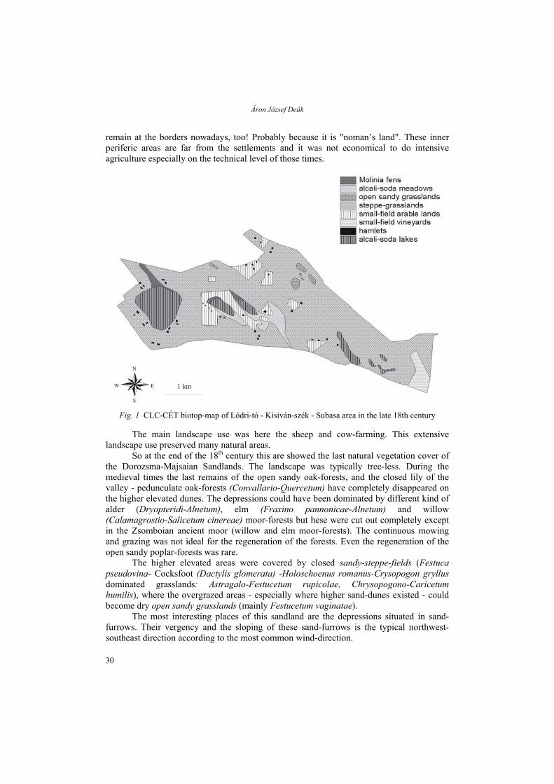
Áron József Deák
remain at the borders nowadays, too! Probably because it is "noman’s land". These inner periferic areas are far from the settlements and it was not economical to do intensive agriculture especially on the technical level of those times.
1 km
Fig. 1 CLC-CÉT biotop-map of Lódri-tó - Kisiván-szék - Subasa area in the late 18th century
The main landscape use was here the sheep and cow-farming. This extensive
landscape use preserved many natural areas. So at the end of the 18th century this are showed the last natural vegetation cover of
the Dorozsma-Majsaian Sandlands. The landscape was typically tree-less. During the medieval times the last remains of the open sandy oak-forests, and the closed lily of the valley - pedunculate oak-forests (Convallario-Quercetum) have completely disappeared on the higher elevated dunes. The depressions could have been dominated by different kind of alder (Dryopteridi-Alnetum), elm (Fraxino pannonicae-Alnetum) and willow (Calamagrostio-Salicetum cinereae) moor-forests but hese were cut out completely except in the Zsomboian ancient moor (willow and elm moor-forests). The continuous mowing and grazing was not ideal for the regeneration of the forests. Even the regeneration of the open sandy poplar-forests was rare.
The higher elevated areas were covered by closed sandy-steppe-fields (Festuca pseudovina- Cocksfoot (Dactylis glomerata) -Holoschoenus romanus-Crysopogon gryllus dominated grasslands: Astragalo-Festucetum rupicolae, Chrysopogono-Caricetum humilis), where the overgrazed areas - especially where higher sand-dunes existed - could become dry open sandy grasslands (mainly Festucetum vaginatae).
The most interesting places of this sandland are the depressions situated in sand-furrows. Their vergency and the sloping of these sand-furrows is the typical northwest-southeast direction according to the most common wind-direction.
30

Landscape changes of the Lódri-tó - Kisiván-szék - Subasa area in the Dorozsma-Majsaian Sandlands
Recent reserches pointed out that in one depression both the alcali-sodic and the fen (partly moor) vegetation can appear! My observation shows that the northwest side of the wind-furrow is mainly dominated by moors or Molinia fens (Succiso-Molinietum) (non-alcali sodic vegetation), whereas the southeastern part of the same depression is covered by alcali sodic vegetation. The moors could appear rarely in the past too, as the natural forest cover was lost and it began to dry out (the evapotranspiration increased), and the conditions were ideal just for the fens, but during the humider and cooler periods of the past (small ice ages) the moor could be more frequent in such geographical positions. This unique vegetation appearence of the moor and Molinia fen vegetation is named by me: fen-head, while the alcali-sodic part of the same depression is called: alcali-sodic foot.
The vegetation changes according to the Na-content gradient of the soil: the fen-head contains less Natrium whereas the alcali-sodic foot has more Na. So the Molinia fens changes first at the alcali-sodic foot to an Agrostis stalonifera, Festuca pratensis or Festuca arundinacea dominated alcali-soda meadow, then to a more alcali-sodic Puccinellia limosa alcali-sodic-cape-vegetation in the most sodic parts. As these sand-furrows slopes from the northwest to the southeast the water migrates to the southeastern part of the depressions, where it's collected, as these depressions are mainly without an outlet. As a result of it alcali-soda lakes are formed on the deepest part of the depressions (usually in the SE part). If the water remains for a longer time (regulary until May or June) in the depressions Bolboschoenus maritimus dominated alcali-soda swamps are formed on the shore, but if it dries out soon (by the end of the spring) only the Puccinellia limosa dominated alcali-sodic-cape-vegetation can appear.
According to our oppinion the ground-water is a mixed water. It appears on the surface or near-to the surface at the fen-heads (upper part of the depressions) because of the sloping of the deposit-layers (NW-SE). After then the water flows further according to the sloping slowly to the somewhat lower elevated southeastern part of the depressions. During this time the evapotranspiration affects these solution and it becomes concentrated, its pH increases. Until the boundary of its solution-capacity it can dissolve more salt from the near-to-surface layers and transport them further to the southeast. The salt-content is unloaded when the water is completely evapotranspirated. This could be the reason for the Na-gradient between the low-Na contented fen-head and the more alcali-sodic foot regions.
This phenomene was discribed on this study area at the Kisiván-szék and Sáros-szék, but at Lodri-tó can be seen too with a difference. Here the lake could have 2 soil-water well: one on the northeastern, one on the north edge of the square shaped depression. Here the Molinia fens are laying on the southwestern and the northeastern side of the depression according to the typical above mentined vergency.
In this area significantly more alcali-soda lake existed in the 18th century: Lódri-tó, Kisiván-szék, Sáros-szék, Nagyszék-tó, Vereshomoki-tó.
Small arable lands were existed mainly in the surrounding of Kisivánszék. Just few hamlets were there in those times, but vineyards were established in Subasa.
By the mid-19th century (Fig. 2) the human impact became stronger, as the position of Szeged increased with the growing population and the start of the industrialization. Except Vereshomoki-pasture and Sziksóstó area all the steppe-fields (base-matrix of the landscape) was broken up. Beside the small-field arable lands 4 patches of vineyards also were established to set the sand (Kisdónát-hegy, Csontos-hegy, Ördög-hegy, Széktói-szőlő). Next to the arable lands many hamlets and extended vineyards appeared. The group of the hamlets were called: Kapitányság (District). The searched area belonged copletely to the Domaszéki Kapitányság. The Kiskundorozsma (southeastern part of Kiskunság District)
31

Áron József Deák
was connected to Csongrád county in 1886. The area of the Molinia fens and alcali-soda lakes remained the same.
1 km
Fig. 2 CLC-CÉT biotop-map of Lódri-tó - Kisiván-szék - Subasa area in the mid-1860s
It is interesting that even bigger spontaneous steppe-forests appeared at
Vereshomoki-tó. These forests could have been at the beginning of the succession: white poplar dominated sandy forests could be there (similar as nowadays the Ásotthalom Memory Forest Nature Reserve).
The beginning of the 20th century (Fig. 3) is the golden ages for Szeged in the Austrian-Hungarian Monarchy. The so called Southern Sandland Railway gave a further possibility for the people living in the hamlets, so the number of hamlets increased further as their product could be put to the market easily by the railway. The Filoxera disease caused heavy demages in the vineyards of the Sandlands. The 3rd military survey shows sometimes woodening, or grassing abandoned vineyards. Some of these vineyards were cut out and on their place orchards were established. During this time the intensive cultures of vegetable production (famous Szegedian red pepper) became prefered too. All these processes reduced the area of the sandy steppe-fields. But Molinia fens, and alcali-sodic meadows and swamps existed further.
The 2002 map shows the results of the landscape changes of the last 100 years (Fig. 4). During the socialism the authority tried everything to demolish the word of hamlets. New settlements were established (Domaszék, Bordány, Zsombó). Even though this hasn't attrackted everybody, and later it's become clear that fruits and vegetables can be produced in hamlets effectively. During the last 20 years new recreation settlements (dominated by houses, gardens, orchards or vineyards) grew up (Subasa, Vereshomok, Sziksóstó) which mean more environmental risk, as the sewage and waste problems are unsolved. The
32

Landscape changes of the Lódri-tó - Kisiván-szék - Subasa area in the Dorozsma-Majsaian Sandlands
socialism hasn't influenced much the size of the arable land: small scale arable lands dominate the sandlands because of the geomorfology of the landscape (wind-furrows and dunes).
1 km
Fig. 3 CLC-CÉT biotop-map of Lódri-tó - Kisiván-szék - Subasa area at the beginning of the 20th
century
Nowadays more and more arable lands and vineyards and orchards are given up. All the large-field socialis-type of orchards and vineyards are cut out in this sample area. On the abandoned lands the succession has started. The Dorozsma-Majsaian Sandlands shows a very good regeneration potential comparing this area with the other sandlands of Hungary. It means that all the abandoned lands are covered at least with some degradated Agropyron repens grassland. The ratio of the invasive species is under the national average. On areas where grazing or mowing is regular, the regeneration of the sandy steppe-grasslands is faster. On a 10 year-old fallow Dactylis glomerata-Festuca pseudovina dominated grasslands could appear. If the regeneration reaches a higher level Holoschoenus romanus and Stipa species could appear. The regeneration of the Chrysopogono-Caricetum humilis community is not so good, as it would require more water.
Nowadays the main problem of the Dorozsma-Majsaian Sandland is the decreasing ground-water level. The decrease is 2-6 meters. There are 3 resons for it:
1. During the socialism many draining channels were built to reduce the risk of inland water and gain more arable lands. It meant that the former depressions with fens, alcali-soda lakes or alcali sodic vegetation became to dry out to a steppe-field as all the standing-water is led away quickly. Many local inhabitants said that they were swimming in these depressions 30 years before! The disappearance of the alcali-sodic lake was the biggest landscape change in the Dorozsma-Majsaian Sandlands during the socialism.
33

Áron József Deák
2. There is less precipitation, and we had the 8 warmest year in the last 10 years during last 100 years period here in Szeged.
3. The landscape use: after the privatisation the intensive vegetable cultures became popular, but they require much water. So the farmers dig huge ponds, which are all evaporation windows decreasing the ground-water level further. These watering-holes make more alcali-sodic their surroundings.
1 km
Fig. 4 CLC-CÉT biotop-map of Lódri-tó - Kisiván-szék - Subasa area in 2002
The process of the degradation of the vegetation in the sandland connected to the
out-drying is the following: the moors first became Molinia fens. After then if there is no sodification it's transformed into a sandy steppe-grassland. If there is sodification it is transformed to an alcali-sodic meadows. If the alcali-sodic meadow is leached later the Festuca pseudovina appears and is transformed to degradated steppe-field. If there is plus accumulation of organic materials the alcali-soda field becomes to an Agropyron repens-Festuca pseudovina grassland. If the accumulation of organic material happens on the Molinia fen, it changes into reeds. This accumulation is due to the loss of mowing, or to the infiltration of manure. The sandy steppe-fields, and the alcali-sodic biotops are attacked by an agressive introduced invador tree: the Eleagnus angustifolia. North from Szeged very huge forest of them exists. This tree was introduced to plant forests on sodic soils, but it has broken out. In this area the Asclepias syriaca is not as big problem as at other sandlands of Hungary, but it can spread easily if a grassland is broken up.
This area is not well forested. Unfortunately the most common chosen tree species are: the Locust-tree (Robinia pseudo-acacia), the Austrian Black Pine (Pinus nigra) and the cultivated poplar types. All these species are landscape-alien.
34

Landscape changes of the Lódri-tó - Kisiván-szék - Subasa area in the Dorozsma-Majsaian Sandlands
I studied the connection between soils and biotops according to Géczy’s map of genetical soil-types published by Keveiné Bárány (1988) and the genetical soil map of the National Atlas (Pécsi, 1989).
According to these maps the sandy steppe-grasslands can be found on different kinds of chernozem soils formed on sand or highly humic sand. The chernozem soils formed on sands are mainly arable lands dominated by cereal production. The majority of the steppe-vegetation remained mainly on such places where the soils with higher organic content are enclosed in alkali-sodic or boggy areas.
The majority of these slightly humic sand dominated areas are forested with Scotch and Austrian Black Pine, Locust Tree, cultivated and native poplar species or became the place of fruit- and vegetable-production, so the open dry sandy grasslands disappeared.
The depressions of the Dorozsma-Majsaian Sanlands have either carbonated and moor-meadow soils - where the Molinia fens are typical - or are dominated mainly by carbonated solonchak, callous solonetz or solonetzic meadow chernozem. The alcali-sodic areas are covered with Achillea (Achillea-Festucetum pseudovinae) alcali-soda grasslands, and with alcali-soda meadows and swamps.
CONCLUSION
These mapping works are useful for nature conservation and we get a full picture of the present and past feature of the landscape. The presented maps can be a database for monitoring and planing the landscape and are good for purposes of rural development, forest and water management. They show the areal potential of rural ecotourism and helps the environmental education. They help the scientific experts, the policy-makers and land-users to make optimal decisions and do a really sustainable landscape use (Dobrosi et al., 2002).
The regeneration potential of the landscape is relatively high, but the landscape is waiting for help. The reintroduction of the traditional extensive grazing and mowing could help the regeneration of the steppe-grasslands. The degradation of the Molinia fens, alcali-soda meadows could be stopped with better water regulation. Today nobody is responsible for it, and the farmers are still affraid of the high water-levels in the early springtime and lead the water with channels away. But in the early-comming hot summer period they don't have enough water and they have to use water from the decreasing ground-water table. It means, that more and more water should be kept in the depressions former alcali-soda lakes. It would help the humider vegetation to survive, but also could increase the decreasing ground-water.
To all these purpuses environmentally sensitive agricultural and landscape planning is required. Unfortunatelly so far the local agricultural policy wasn't so nature-friendly. But in the EU we should try to do such an agriculture which is good for the nature too. To make this a reality the environmental consciousness must be improved on local and decision-making level too.
REFERENCES
ÁESZ, 1998: Kistelek-Sándorfalvi körzet erdészeti üzemterve (Forestry Plan of the Kistelek-Sándorfalva district).
Állami Erdészeti Szolgálat, Szeged. Bölöni, J., Kun, A. and Molnár, Zs., 2003: Élőhelyismereti Útmutató 2.0 (Biotop Guide 2.0 for the Hungarian
vegetation). MÉTA program anyag, MTA-ÖBKI, Vácrátót, manuscript.
35

Áron József Deák
Dobrosi, D., Deák, J. and Deák, J.Á., 2002: A Csongrád-Nagyréti Természetvédelmi Terület természetvédelmi kezelési terve (Treating plan of the Csongrád-Nagyrét nature reserve). Csongrád, manuscript.
Fekete, G., Molnár, Zs. and Horváth, F. (eds.), 1997: Nemzeti Biodiverzitás-monitorozó Rendszer (II.): Magyarországi élőhelyek (National Biodiversity Monitoring System II: Hungarian biotops). Magyar Természettudományi Múzeum, Budapest.
Gauss-Krüger topographical maps (L 34-64-B-b, L-34-64-A-a), 1992: Scale: 1:25,000, Magyar Honvédség Tóth Ágoston Térképészeti Intézet, Budapest.
Kaán, K., 1931: Természetvédelem és a Természeti Emlékek. (Nature conservational values and memories) Keveiné Bárány, I., 1988: Talajföldrajzi vizsgálatok Szeged környékén (Soilgeographical researches int he
surrounding of Szeged). Alföldi Tanulmányok. Békéscsaba, 25-31. Kincsek, I. 1996: Ásotthalmi Láprét Természetvédelmi Terület (Ásotthalmian Fen Nature Reserve). Agapé Kft.,
Szeged. Margóczi, K., Urbán, M. and Szabados, B., 1998: "Csodarétek" a Dél-Kiskunságban (Wonder fields int he
Southern-Kiskunság). Kitaibelia III/2, 275-278. Molnár, Zs. and Horváth, F., 2000a: CORINE Land Cover (CLC), CLC50 nomenklatúra 1.4., Földmérési és
Távérzékelési Intézet, Budapest, manuscript. Molnár, Zs. and Horváth, F., 2000b: m-ÁNÉR élőhelylista (Biotop-list of the modified General National Biotop
Classification System). Gólyahír III/13., IBOA-s szám. 8-10. Molnár, Zs. and Horváth, F., 2001: CÉT kategóriái (Categories of CÉT). MTA-ÖBKI, Vácrátót, manuscript. Mucsi, S. (ed.), 1990: Magyarország kistáji katasztere I. (Cataster of the Hungarian small landscapes), Magyar
Tudományos Akadémia Földrajzi Kutató Osztály, Budapest, 83-86, 210-218. Maps of the 1st military survey (1764-1787), Scale: 1:28,000. Magyar Királyi Térképészeti Intézet, Vienna
(Source: Hadtörténeti Múzeum Térképtára, Budapest). Maps of the 2nd military surves (1806-1869), Scale: 1:18,000, Magyar Királyi Térképészeti Intézet, Vienna,
(Source: Hadtörténeti Múzeum Térképtára, Budapest). Maps of the 3st military survey (1872-1887), Scale: 1:75,000, Magyar Királyi Térképészeti Intézet, Vienna,
(Source: Hadtörténeti Múzeum Térképtára, Budapest). Maps of the Hungarian forest-management plans, 1998, Scale: 1:20,000. (Source: Állami Erdészeti Szolgálat,
Szeged). Pécsi, M. (ed.), 1989: Magyarország nemzeti atlasza (National Atlas of Hungary). Kartográfiai Vállalat, Budapest. SPOT4 satelite images, 1998: (Source: MÁFI, Budapest, MTA-ÖBKI, Vácrátót). Tardy, J. (ed.), 1996: Magyarországi települések védett természeti értékei (Protected natural values of the
Hungarian settlements). Mezőgazda Kiadó, Budapest, 171-172, 179, 181.
36
ACTA CLIMATOLOGICA ET CHOROLOGICA Universitatis Szegediensis, Tom. 36-37, 2003, 37-44.
ANALYSIS OF THE BIOCLIMATIC CONDITIONS WITHIN DIFFERENT SURFACE STRUCTURES IN A MEDIUM-SIZED CITY (SZEGED, HUNGARY)
Á. GULYÁS1, J. UNGER1, B. BALÁZS1 and A. MATZARAKIS2
1Department of Climatology and Landscape Ecology, University of Szeged, P.O.Box 653, 6701 Szeged, Hungary E-mail: [email protected]
2Meteorological Institute, University of Freiburg, Freiburg im Breisgau, Germany
Összefoglalás – A városklíma kutatásokon belül a humán bioklimatológia napjaink egyik legdinamikusabban fejlődő részterülete. Az utóbbi években számos indexet fejlesztettek ki annak számszerűsítésére, hogy mekkora az emberi szervezetet érő hőterhelés különböző környezetben, illetve milyenek az emberi test és a környezete közötti energiaáramlási viszonyok. Jelen vizsgálatunkban egy esettanulmányt mutatunk be Szeged (160 000 lakosú város Magyarország délkeleti határszélén) példáján, melyben egy kis mintaterület bioklimatikus viszonyait elemezzük. Bioklimatológiai szempontból alapvető fontosságú, hogy a vizsgált test direkt sugárzásnak kitett, vagy árnyékban lévő ponton helyezkedik-e el. Mintaterületünk a város magas beépítettségű belvárosi régiójában található, szűk utcakanyonok jellemzik, 20-30 éves (20-30 m magas) útszéli fasorral. A sugárzási viszonyok tehát ezen feltételeknek megfelelően módosulnak. Tanulmányunkban bemutatjuk, hogy hogyan reagálnak a különböző bioklíma indexek-értékek (például a PMV-Predicted Mean Vote és a PET-Physiological Equivalent Temperature) a felszíni struktúra megváltoztatására. Az indexszámításokat RayMan modell segítségével végeztük. Summary - Human biometeorological approaches have an important role in applied urban climatology. Several different thermal indices were developed in the last decades to describe human comfort or heat stress of the human body based on the energy fluxes between the body and environment. In this study some results of recent biometeorological investigations in a south-eastern Hungarian city, Szeged (population 160,000) are presented. From point of view of human biometeorology, the key question is whether the examined body is in the shade or is exposed to direct radiation. Our sample area is in a heavily built-up city centre region with narrow streets and several 20-30 year old (20-30 m tall) trees, so radiation fluxes are determined basically by these factors. This paper shows how the bioclimatic indices, Predicted Mean Vote (PMV), Physiological Equivalent Temperature (PET) depend on the situation of radiation at a certain place. It was examined what is the relation between the structure and possible changes of the built-up area and the indices. All the calculations, Tmrt, PMV and PET were performed with RayMan model.
Key words: radiation fluxes, thermal comfort, mean radiant temperature, Predicted Mean Vote, Physiological Equivalent Temperature, Szeged, Hungary
INTRODUCTION
One of the environmental stress factors on human being living in the urban area is the effect of partly artificial climate conditions, which are formed mainly by the area’s building up.
An important task of the bioclimatological research to evaluate thermo-physiologically the thermal and radiating environment of human beings, because it determines basically the energy balance of the body (Höppe, 1993). The physiologically relevant assessment of urban climate, and especially different urban microclimates, requires
37

Ágnes Gulyás, János Unger, Bernadett Balázs and Andreas Matzarakis
the use of methods and indices, which combine meteorological elements with personal parameters (Mayer, 1993; VDI, 1998). Human comfort issues and quantitative bioclimatological indices generate valuable information for urban planners, helping them to increase the well-being of urban population by planning suitable and healthy environment.
This study is based on earlier bioclimatic and recent urban climatological studies in a Hungarian city, Szeged. Recent studies show that on annual average an urban heat island intensity of 2.7ºC can be measured in Szeged which can extend up to 6.8ºC at clear, anticyclonal weather conditions (Sümeghy and Unger, 2003). It means a significant heat-stress to the human body, especially in summer. In the earlier bioclimatic studies, with the help of suitable indices for the available data set, differences in the annual and diurnal variation of human bioclimatic characteristics between an urban and rural environment were evaluated over a 3-year period (Unger, 1999). According to the results, the city favourably modifies the main climatological elements within the general climate of its region; periods likely to be comfortable are therefore found more frequently in the city than in rural areas.
STUDY AREA AND METHODS
Study area
Szeged is located in the south-eastern part of Hungary (46ºN, 20ºE) at 79 m above sea level on a flat plain, with a population of 160,000 (Fig. 1B). As Fig. 1C shows the city has a boulevard-avenue road system, with several different land-use types from the densely built centre to the detached housing in the suburb regions. Fig. 1D – created by the RayMan model – shows the area of investigation (200 x 200 m) in the heavily built-up city centre region with narrow streets and several 20-30 year old (20-30 m tall) deciduous trees.
A
B
C
D
Fig. 1 Geographical location of Hungary in Europe (A), of Szeged in Hungary (B), the road network of the city (C) and the investigation area (D) with fixed measurement site in its centre (•) created by the RayMan model. The buildings are marked by light grey and trees by dark grey on the part of D.
38

Analysis of the bioclimatic conditions within different surface structures in a medium-sized city (Szeged, Hungary)
Parameters and methods
Lots of models were developed to estimate the radiation fluxes, and the energy balance of human body in different environments, including various meteorological parameters, albedo of the surface and solid angle proportion (Fanger, 1972; Gagge et al., 1971; Höppe, 1999; Matzarakis et al., 2000a; Spagnolo and de Dear, 2003). The models use complex comfort indices − for example Predicted Mean Vote (PMV) and Physiological Equivalent Temperature (PET) − to evaluate the thermal stress on the body. Most of the indices are based on mean radiant temperature (Tmrt), which is the most important input parameter for the energy balance during sunny weather (Matzarakis et al., 2000b). Tmrt is defined as ”the uniform temperature of a surrounding surface giving of blackbody radiation (emission coefficient ε=1) which results in the same energy gain of a human body as the prevailing radiation fluxes” (Matzarakis et al., 1999).
PMV predicts the mean assessment of the thermal environment for a large sample of human beings by value according to the seven-step ASHRAE comfort scale (in really extrem weather situation PMV can be higher than 3.5, or lower than -3.5) (Höppe, 1993 and 1999; Mayer and Matzarakis, 1997,).
PET is one of the most popular and useful bioclimate index, because it has a widely known unit (ºC), which makes results easy understandable and comprehensible for urban planners and decision-makers. PET is defined as the air temperature at which the human energy balance for the assumed indoor conditions is balanced by the same skin temperature and sweat rate as the calculated for the actual outdoor conditions (Mayer and Matzarakis, 1997).
One of the recently used bioclimatical model is the RayMan model, which is well-suited to calculate radiation fluxes because it considers more precisely the effect of a complex urban structure (Matzarakis, 2002).
ap
Table 1 Comparison of PMV (Predicted Mean Vote) and PET (Physiological Equivalent Temperature) ranges for different human sensations and thermal stress level by human beings.
(internal heat production: 80 W, heat transfer resistance of the clothing: 0.9 clo) (Matzarakis et al., 1999)
PMV PET (°C) Human sensation Thermal stress level very cold extreme cold stress
Among others a final output of the model is in polar co-ordinates about the area including the sun path of the observation day at the place, with the shadow of buildings, trees, or other obstacles and sky view factor. All our calculations, Tmrt, PMV and PET were performed with this model.
A 3-D map of the examined area was made with the help of RayMan model, which gives precise
nd high resolution data of the surrounding area of the observation point. Meteorological arameters (air temperature, global radiation, wind speed and relative humidity) were
-3.5
-2.5
-1.5
-0.5
0.5
1.5
2.5
3.5
4 8
13
18
23
29
35
41
…………… cold
…………… cool
…………… slightly cool ……………. comfortable ……………. slightly warm …………….
warm …………….
hot …………….
very hot
……………… strong cold stress ………………
moderate cold stress ………………. slight cold stress ……………….
no thermal stress ……………….. slight heat stress ………………..
moderate heat stress ……………….. strong heat stress ………………..
extreme heat stress
39

Ágnes Gulyás, János Unger, Bernadett Balázs and Andreas Matzarakis
logged by a VAISALA-MILOS 500 automatic weather station, which is located at the centre of the investigation area marked with (•) on Fig. 1D.
10
15
20
25
30
35
0:10
3:10
6:10
9:10
12:10
15:10
18:10
21:10
time
air
tem
pera
ture
(o C)
20
30
40
50
60
70
rela
tive
hum
idity
(%)
Ta
RH
00.5
11.5
22.5
33.5
44.5
5
0:10
3:10
6:10
9:10
12:10
15:10
18:10
21:10
time
wind
spe
ed (m
/s)
0100200300400500600700800900
glob
al ra
diat
ion
(W/m
2 )WS_rWS_sGR_r
Fig. 2 Diurnal courses of meteorological parameters on 4th August 2000 (WS_r: wind speed on the roof, WS_s: wind speed at the surface, GR_r: global radiation, Ta: air temperature, RH: relative
humidity)
Fig 2 shows the diurnal courses of the meteorological parameters, which can characterise the weather conditions of the observed day (4th August 2000). The temperature increased rapidly during the morning hours due to the undisturbed sunshine (global radiation). The maximum temperature was 32.7°C, so that was a hot summer day with − especially at the surface − low wind speed. The minimum air temperature during the night was respectively 19.0 °C.
RESULTS AND DISCUSSION
The bioclimatic situation at the observation point was examined in four cases: - case A (t+b): real situation considering trees and buildings (Fig. 3A), - case B (b): hypothetical situation with buildings only (Fig. 3B), - case C (t): hypothetical situation with trees only (Fig. 3C), - case D (r): without any obstacles like the “roof region” of the buildings (sky view factor = 1).
The calculated obstacle structures in the first three cases are shown in polar co-ordinates, as an output of RayMan (Fig. 3). There are notable differences in the radiation conditions between the three situation: on the one hand due to different sky view factors (case A: 0.278, case B: 0.431, case C: 0.560), on the other hand the shading of direct radiation by obstacles.
By model calculated PMV and PET values are shown on Fig. 5A and Fig. 5B, respectively. Heat stress was experienced on the examined day: the highest value of PET was 46.8ºC; and in the case of PMV the scale (based on the ASHRAE scale) was 4.4, which means ”very hot” thermal stress level. The shapes of the courses have almost the same form as Tmrt. That was not an unexpected result, because the part of Tmrt is primary factor of heat stress. The Tmrt values were the highest on the roof between 10 a.m. and 1 p.m., because of the strong, undisturbed direct and diffuse radiation. On the other hand the
40

Analysis of the bioclimatic conditions within different surface structures in a medium-sized city (Szeged, Hungary)
PMV and PET indices were at this time the lower on the roof. It was caused probably by the higher wind speed on the roof than at the surface (Fig. 2).
Fig. 3 Output fisheye diagram about the investigation area with buildings and trees (A), with only buildings (B), with only trees (C) and the sun path on 4th August 2000, for the calculation of the sky
view factors in RayMan
Estimated Tmrt values based on the model are shown on Fig 4. Because Tmrt values have strong correlation with global radiation values and there was undisturbed sunny day on the day of measurement; significant alterations in the shape of curves caused mainly by the situation when the observation point was shaded or hit by direct radiation. After the sunrise Tmrt values increased quickly on the roof (“Tmrt_r”) with sky view factor of 1 and in the case of trees only (“Tmrt_t”). In the two other cases the increase begins only at 9 am, when the direct radiation hit the hypothetical body. The degree of the observed fast increase is around 30°C. The shapes of the curves are similar at noon because direct radiation hit the body in all cases, but there is a difference in the maximum values. The absolute maximum value is 62.3°C in the case of “Tmrt_r”, while at the same time this value exceeds only 59.9°C in the case of “Tmrt_t+b” which means real surface structure. This difference is caused by the different projection factor.
41

Ágnes Gulyás, János Unger, Bernadett Balázs and Andreas Matzarakis
10
20
30
40
50
60
0:10
3:10
6:10
9:10
12:10
15:10
18:10
21:10
time
Tm
rt (o C
)
Tmrt_t+bTmrt_bTmrt_tTmrt_r
Fig. 4 The mean radiant temperature Tmrt computed by RayMan in the three urban structures and on
the roof on 4th August 2000
-1.5
-0.5
0.5
1.5
2.5
3.5
4.5
0:10
1:10
2:10
3:10
4:10
5:10
6:10
7:10
8:10
9:10
10:10
11:10
12:10
13:10
14:10
15:10
16:10
17:10
18:10
19:10
20:10
21:10
22:10
23:10
time
PMV
PMV_t+bPMV_bPMV_tPMV_r
10
15
20
25
30
35
40
45
50
0:10
1:10
2:10
3:10
4:10
5:10
6:10
7:10
8:10
9:10
10:10
11:10
12:10
13:10
14:10
15:10
16:10
17:10
18:10
19:10
20:10
21:10
22:10
23:10
time
PET
(o C)
PET_t+bPET_bPET_tPET_r
Fig. 5 Predicted Mean Vote PMV and Physiological Equivalent Temperature PET in the three urban
structures and on the roof on 4th August 2000
42

Analysis of the bioclimatic conditions within different surface structures in a medium-sized city (Szeged, Hungary)
CONCLUSIONS
The following conclusions are reached from the analysis presented: (i) The presence of natural and artificial obstacles around the human body has
impact on the radiation fluxes so on the energy balance of the body. (ii) Changes in the radiation situation cause changes in thermal comfort perception. (iii) Disadvantageous bioclimatic conditions can be improved (e.g. planting trees)
even in the case of old ”inherited” city structure. (iv) In the course of planning of new districts in a city bioclimatic conditions must
be taken into consideration.
Acknowledgements – This research was supported by the grant of the Hungarian Scientific Research Fund (OTKA T/034161). The work of the second author was also supported by the Széchenyi István Scholarship of the Ministry of Education (SZÖ 84/2002). The Fig. 1A-C was drawn by Z. Sümeghy.
REFERENCES
Fanger, P.O., 1972: Thermal comfort. Mc Graw-Hill, New York. Gagge, A.P., Stolwijk J.A.J., Nishi, Y., 1971: An effective temperature scale based on a simple model of human
physiological regulatory response. ASHRAE Trans 77, 247-257. Höppe, P.R., 1993: Heat balance modelling. Experientia 49, 741-745. Höppe, P.R., 1999: The physiological equivalent temperature – a universal index for the biometeorological
assessment of the thermal environment. Int. J. Biometeorol. 43, 71-75. Matzarakis, A., Mayer, H. and Iziomon, M., 1999: Applications of a universal thermal index: physiological
equivalent temperature. Int. J. Biometeorol. 43, 76-84. Matzarakis, A., Rutz, F. and Mayer, H., 2000a: Estimation and calculation of the mean radiant temperature within
urban structures. In: Biometeorology and Urban Climatology at the Turn of the Millenium (ed. by de Dear, R.J., Kalma, J.D., Oke, T.R. and Auliciems, A.): Selected Papers from the Conference ICB-ICUC’99, Sydney, WCASP-50, WMO/TD No. 1026, 273-278.
Matzarakis, A., Rutz, F. and Mayer, H., 2000b: Importance of the mean radiant temperature on thermal conditions of humans in urban areas. 3rd Japanese-German Symposium on Urban Climatology, Essen-Germany, 41-42.
Matzarakis, A., 2002: Validation of modelled mean radiant temperature within urban stuctures. AMS Symposium on Urban Environment, Norfolk, USA, 7.3.
Mayer, H., 1993: Urban bioclimatology. Experientia 49, 957-963. Mayer, H. and Matzarakis, A., 1997: Human-biometeorological assessment of urban microclimates’ thermal
component. Proceedings of the Int. Symposium on Monitoring and Management of Urban Heat Island, Fujisawa-Japan, 155-168.
Spagnolo, J. and de Dear, R., 2003: A field study of thermal comfort in outdoor and semi-outdoor environments in subtropical Sydney Australia, Building and Environment 38, 721-738.
Sümeghy, Z. and Unger, J., 2003: Classification of the urban heat island patterns. Acta Climatologica et Chorologica Universitatis Szegediensis 36-37 (this issue), 93-100.
Unger, J., 1999: Comparisons of urban and rural bioclimatological conditions in the case of a Central-European city. Int. J. Biometeorol. 43, 139-144.
VDI, 1998: Methods for the human-biometerological assessment of climate and air hygiene for urban and regional planning. Part I: Climate. VDI guideline 3787. Part 2. Beuth, Berlin.
43


ACTA CLIMATOLOGICA ET CHOROLOGICA Universitatis Szegediensis, Tom. 36-37, 2003, 45-56.
COMPARISON OF ARTIFICIAL INTELLIGENCE PREDICTION TECHNIQUES IN NO AND NO2 CONCENTRATIONS' FORECAST
I. JUHOS1, R. BÉCZI2 and L. MAKRA2
1Department of Informatics, University of Szeged, P.O.Box 652, 6701 Szeged, Hungary E-mail: [email protected]
2Department of Climatology and Landspace Ecology, University of Szeged,P.O.Box 653, 6701 Szeged, Hungary
Összefoglalás – A műszaki eszközök és berendezések, valamint az épületek védelme iránti állandó igény, továbbá az az elvárás, hogy a gazdasági és gazdálkodási folyamatok költségeit csökkentsük, egyre pontosabb előrejelzési technikákat igényelnek. Az előrejelzés nehéz probléma, mellyel csaknem minden emberi tevékenység szembesül. Kifejlesztettek ugyan számos speciális idősor előrejelzési módszert, ezek mindegyikének azonban vannak bizonyos korlátai. Legtöbbjük sokkal inkább teljes adatsorok modellezésére korlátozódik, semmint az előrejelzési sajátosságok kiemelésére és a terület szakemberei számára általában nehezen értelmezhetők. A mesterséges intelligencia a döntési fákkal történő szimbolikus tanulást ajánlja, mely lehetőséget biztosít a múltbeli adatokban rejlő kapcsolatok felderítésére, számunkra is olvasható formában. Mindezek mellett képes megbecsülni azt, hogy a jövőbeli adatok milyen intervallumba esnek. Precízebb előrejelzést az elmúlt években erre a problémára legtöbbet használt mesterséges neurális hálózatok segítségével nyerhetünk, amelyek pontos függvényillesztést végeznek az adatokon. Ennek ára azonban az összefüggések emberi szem elől való elrejtése. Ha az említett módszerek kombinációját használjuk, akkor pontosabb döntésekre juthatunk a jövőbeni adatokra vonatkozóan, továbbá az okokat is feltárhatjuk. Mindkét esetben a tanulás hatékonysága a tanulóalgoritmusok paramétereinek jó megválasztásától függ. Emiatt a paraméterek beállítására szimulált hűtéssel felügyelt tanulást alkalmaztunk. A dolgozat célja, hogy összehasonlítsuk a fent említett technikákat az NO és NO2 koncentrációk néhány órás előrejelzésében egy forgalmas szegedi közlekedési csomópontban. Ehhez az aktuális értékeik alapján adott hibával előrejelzett meteorológiai paramétereket hívtunk segítségül. Summary – To construct new technical devices, to permanently protect buildings and to reduce the expenses of various economic and business processes more and more accurate prediction techniques are needed. Almost all human activities encounter the hard problem of forecasting. Although several time series prediction methods have been developed, each of them has certain limitations. Most of them are designed rather for modeling complete time series than pointing out different prediction characteristics; furthermore, they can only be interpreted with difficulties. Artificial intelligence offers symbolic learning with decision trees, by means of which we can explore connections in past data and produce them in a readable format. Decision trees can estimate intervals of future data. Recently, artificial neural networks were used to handle this problem. This method offered more precise forecast and more accurate fit of the function to the starting data. However, when applying this method, relationships in the data set examined were hidden. If we combine the methods mentioned above, we can get more precise decisions for the future data and we can also reveal the reasons. In either case, the efficiency of learning depends on a good choice of the learning algorithms' parameters. For this reason, parameters are selected by simulated annealing. The aim of this paper is to compare the above mentioned prediction techniques in several hours forecast of NO and NO2 concentrations at a busy cross-road in Szeged (Hungary). For this object, meteorological parameters predicted with given error on their actual values were used.
Key words: NO and NO2 concentrations, neural network, decision tree, forecast, prediction
INTRODUCTION
Considering the special meteorological and geographical conditions of Szeged, dispersion of air pollutants – especially during permanent anticyclone weather conditions in
45

István Juhos, Rita Béczi and László Makra
the summer and winter seasons – is very slow. A reliable forecast of concentrations of the air pollutants is very important. It makes possible for the authorities to prepare people for heavy air pollution episodes. Several authors have used methods using classical statistics as well as methods of neural networks in order to make short term forecast of various gases and particulate matter. Gardner and Dorling (1998) give an excellent account on the applications of neural network methods for forecasting in atmospheric sciences. It is worth to mention here paper of Jorquera et al. (1998), which compares a linear model – a neural network model – and a fuzzy model as a prediction of daily maximum ozone concentrations. Perez et al. (2000) presents an
lication of neural networks for a few hours prediction of PMapp
2.5 in the atmosphere of Santiago city (Chile), where the input data are hourly PM2.5 concentrations in the previous day. Ziomas et al. (1995) analyses the possibility of forecasting maximum ozone concentrations in Athens city. He applied discriminant analysis to forecast possible increase and decline of NO2 levels. He considered the following parameters: previous daily maximum ozone concentration; forecasted temperature; wind velocity and direction; an index of the given day's short term emission change; an index of the effect of the precipitation on the given day. In average, 80 % of the forecasts were successful. If we use multivariate linear regression analysis, these forecasts give quantitative estimates for the maximal hourly averages of NO2 concentrations on the next day.
Maros
Tisza
Tisz
a
Tisza
Körös
Lake Fehér
Lake Csaj
SZEGED
KISTELEK
CSONGRÁD
HÓDMEZŐ-VÁSÁRHELY
MAKÓ
Ásotthalom
ZákányszékAlgyő
Maroslele
0 10 20 30 km
Fig. 1a Geographical position of Szeged, Hungary in Europe (top left); Csongrád county in Hungary (top
right); and Szeged in Csongrád county (centre)
Tisza
1
0 5 km
Fig. 1b The built-up types of Szeged [a: centre (2-4-storey buildings); b: housing estates with prefabricated
concrete slabs (5-10-storey buildings); c: detached houses (1-2-storey buildings); d: industrial areas; e:
green areas, (1): monitoring station]
In this paper, a test is presented and different forecasting methods are compared; furthermore, they are used to forecast hourly averages of NO and NO2 concentrations.
46

Comparison of artifical intelligence prediction techniques in NO and NO2 concentrations’ forecast
DATA BASIS
Data basis of the paper comes from the monitoring station located in Szeged city in a crossroad (Kossuth Lajos Avenue and Damjanich Street). The data basis consists of a five-year data set from the period between January 1, 1997 – December 31, 2001. The elements considered are, on the one hand, the average mass concentrations (µg m-3) of SO2, O3 and PM10 and, on the other hand, the average values of the main climatic elements (temperature, humidity, air pressure, global radiation, wind direction and wind speed). The verified database of the study consists of the 30-minute averages of the above-mentioned pollutants and climatic elements. The monitoring station is operated by the Environmental Protection Inspectorate of Lower-Tisza Region, Szeged, under auspices of the Ministry of Environment, Hungary.
Szeged (20°06'E; 46°15'N) is situated near the confluence of the Tisza and Maros Rivers. It is the largest town in the south-eastern part of Hungary, at about 20 km from Hungarian-Serbian border. The city and its surroundings are flat and low and the elevation is 79 m above sea level, the lowest in the Carpathian basin. The number of inhabitants of the city is up to 160,000 and the territory of its built-up area is about 46 km2 (Fig. 1a-b).
The basis of the city structure is a boulvard-avenue street system crossed by the Tisza River (Fig. 1b). In this way, the structure of the city is simple; however, following to this system, motor vehicle traffic as well as air pollution are concentrated in the city.
The industrial area is found main-ly in the north-west part of Szeged. Thus, the prevailing westerly and northerly winds transport air pollutants, coming from this area, towards the city centre.
METHODS
Inductive learning of atmospheric parameters
Inductive learning of a concept means recognizing a hypothesis regarding this concept after presenting the training instances to the learner. The simplest learning case is that, where one part of the training instances is true (positive) and another part is false (negative). A set of the instances can be regarded as a function. The domain of this function consists of the instances, while the values are either true or false according to the instance. During the training process, the instances are generally at disposal in the following format:
x1, x2, ... , xn, y
instance class where xi is the i-th attribute of the instance and y is the class of the instance (true or false). A training instance and its class is a training example (in certain case an instance phrase is equal to a mentioned example). In order to find the inductive hypothesis, a function of y = h(x1, x2, … , xn) based on the training instances have to be approximated. The number of the classes can be extended to more than two; thus, the problem can be generalized to the classification into more than two discrete classes or to the learning of functions with not discrete range. Goodness of the h hypothesis can be determined by applying it on the not presented instances (which were not in the training set).
47

István Juhos, Rita Béczi and László Makra
The estimate of the atmospheric parameter corresponds to an inductive learning model. Past data are the instances, and the forecast of the data will be determined by an inductive hypothesis. The accuracy of the learning depends on the number and on the accuracy of the training data (data can be come from real process by measurement), while the quality of the learning (the finding of the inductive hypothesis) depends on the chosen learning algorithm.
The accuracy of the meteorological data is determined by measuring instruments. We chose a database of approximately five months for the learning period. The data taken into account are hourly average values of concentrations between 28th February 2003, 00:00 CET to 9th July 2003, 24:00 CET. In the paper artificial neural networks are applied as learning algorithm or machine learner, which are frequently used in this field. To understand the relationships among the data, decision trees were applied.
Decision trees
The decision tree is a tree-graph, vertices of which denote branch points. The branch points are determined by the attributes of the learning instances. The leaves of the tree mean a classification of the learning instances. The applied algorithm of the C4.5 decision tree (Quinlan, 1993) builds up the tree based on the so-called information gain. The gain determines the extent to which an attribute describes the proper classification of a given set of instances; i.e., which decreases mostly the entropy of the classification. If we choose the attribute with the largest gain, the algorithm puts it to the root of the tree. The sub-trees branching from the root are determined following the same procedure from the partition classes given by the chosen attribute. The learning, which is exactly the construction of the tree, stops if we reach the last attribute. This algorithm is working on discrete attribute values but easily extends to real attributes. After the learning, the decision tree is able to classify previously unknown instances. Certain rules between the attributes can be derived from the tree and we can also infer their effect on the decision making. If the tree grows too large, we may loose generality. To avoid this, we can do pruning of the branches of the decision tree. Before building the tree, categories have to be made if the learning class is not discrete. In our case, this particularly means the partitioning of the estimated range into intervals.
Artificial neural network
In this paper estimations are provided for future concentrations by backpropagation multi-layer perceptron (BMLP) 24 hours beforehand (Kaastra and Boyd, 1996). In the hidden layer, sigmoid activation function is used:
xex
−+1
1)(g = (1)
The main task is to approximate the functions. The three-layer BMLP is capable of approximating arbitrary finite sets of real numbers (Hornik et al., 1989). When the attributes of the learning instances take the form xi1, ... , xin then the class of the i-th instance produced by the perceptron is yi = g(w1xi1 + … + wnxin + b) (2)
48

Comparison of artifical intelligence prediction techniques in NO and NO2 concentrations’ forecast
where wj (j = 1, … , n) are the weights of the input layer; b is the threshold of the activation function; g is the activation function.
Overfitting
A general drawback in machine learning is overfitting. When the precision of the approximation of the desired function is increased, the generality may be destroyed. Thus, in case of the instances taken outside of the training set the sum of the errors increases. Generally, these phenomena may be observed in the later phases of the training process. Using a larger training set or stopping the training process in due time may provide a solution to this problem; nonetheless, there are no exact definitions of the correct stopping time. In the case of decision trees, we saw a branch-pruning technique, which could lead to a solution, but which also introduces more and more parameters. It is not determined when or which branch pruning is needed. We see that learning process is significantly influenced by certain parameters, which are usually set through several trials.
Setting of the parameters
Learning, as function of fitting, involves optimization. The function to be optimized has, in general, bad behaviours. It has many parameters and several local extrema, thus the searching algorithms are often stuck in local minimum points. The multi-parameters optimization and the approximation is carried out during the training process (in case of the BMLP it is done using backpropagation), its goodness is the function of certain parameters (in case of BMLP, learning rate used in backpropagation, momentum, etc.) regarding the learners. These are usually determined by experiments. If more precision is required, another optimization is needed but this time not among the training instances rather in the parameter space of our training algorithm; which, of course, depends on the training data.
The heuristic search
We use a heuristic search algorithm to handle and control the above-mentioned problems of overfitting and the setting of training parameters and thus to facilitate a better learning. During this algorithm, we split the historical data set in two parts: a larger set of training and a smaller set of test instances; more exactly, the union of these gives back the original training set. Considering an initial parameterization of our learner, which is installed on a training set, a hypothesis is obtained. We check its correctness on the set of test instances and we measure the error (it is called validation). The error determines a so-called fitness function f depending on the training parameters, the smaller the error is the smaller the values of f are. We try to minimize the fitness function using the heuristic search. Reaching the minimum of f it is plausible that our posed hypothesis is appropriate according to the given data. Using the parameters yielded by the heuristic search, we train our learner again on the union of the sets of training and test instances, i.e., on the historical training set. Thus, using more instances in the training process hypothesis becomes better.
Simulated annealing was applied as heuristic search, which is frequently used in the field of artificial intelligence. This is a quick algorithm, which provides precise estimates on the location of optimum (Nahar et al., 1986).
49

István Juhos, Rita Béczi and László Makra
The simulated annealing
The simulated annealing (SA) is a heuristic method of locating the extrema of functions. In our case, we are looking for the minimum of the fitness function f (or the maximum of 1/f, if it exists). The algorithm has a physical motivation. During the annealing of liquids, the fine structure of the material follows the principle of optimal disposition. There are numerous implementation of SA. We apply a version, which is controlled by the following five parameters: initial temperature, current temperature, minimal temperature (freezing), annealing velocity and maximum number of steps.
Initially we assume that the distance between the elements of the search space (the space of the learners' parameters) is the same; i.e., our assumption is that we have only neighbouring elements. Later, as the temperature falls, the distance between the elements increases according to a coefficient µ depending on the temperature.
We use the Manhattan-distance d to measure the distance between two elements P = (p1, p2, … , pn) and P’ = (p1’, p2’, … , pn’):
∑ −= ppd ')' (3) =
n
iiiPP
1,(
We say that the parameter P' is in the µ- neighbourhood of P, if the following condition holds:
∑=
−<n
iii ppPPd
1
' )min()max()',( µ (4)
where µ = temp / tempmax; temp = actual temperature; tempmax = maximum temperature; max(pi) and min(pi) denote the maximum and the minimum of the possible values of the i-th parameter pi respectively. The function that we would like to optimize is the fitness function f(P). Calculating the value of f for the initial parameter P we decide whether f(P) is an optimum. If not, we continue the procedure with choosing an element P' from the µ-neighbourhood of P. In any case, we accept the step from P to P', if f(P') is better value than f(P). According to SA, we also accept a worse parameter with probability v, which makes it possible that the algorithm leaves local optima. If the better values are only accepted, the search would certainly get stuck in local optima. The probability v depends also on the temperature:
tempv = (5)
PfPf
etemp
)()'(
)(
−
At each step, the temperature falls according to annealing velocity. Reaching the optimum or the maximum number of steps, the algorithm stops and returns the previously found best parameter.
Since the algorithm requires no assumption on the shape of f, it provides a widely applicable tool. Taking small enough decrease in the temperature at each step, we may get sufficiently close to or reach the optima.
50

Comparison of artifical intelligence prediction techniques in NO and NO2 concentrations’ forecast
The SA is used to set the following parameters of the learners. In case of decision trees: it is necessary to apply pruning, pruning threshold and maximal number of nodes in the tree. In case of BMLP: training time, learning rate and moments.
RESULTS
The historical data used in the training are the hourly means of NO, NO2, O3 concentrations and the intensity of global radiation in one-hour steps between 28th February 2001 00:00 CET and 9th July 2001 24:00 CET. The forecasted interval is the period between 10th July 2001, 00:00 CET and 13th July 2001, 24:00 CET, also in one-hour steps.
For the precise estimates we used the 24-1-1 type BMLP (24 input, 1 hidden and 1 output neurons). To explore the relationships between the historical data, the C4.5 decision tree was applied.
Firstly, the attributes of one training instance were the values measured in the 24 hours of a given day (attributes of the instance) and one concentration value of NO or NO2 taken from the following day (class of the instance, i.e., the material which is forecasted) (see Example 1). Then, we added some future external factors measured in the same hour as the data to be predicted. Such factors are the concentration of O3, intensity of the global radiation, and NO2 or NO concentrations depending on which material (NO or NO2) is to be forecasted (see Example 2). Thus, we have two types of estimations, i.e., learning and estimations with or without external factors. Naturally, the future external factors, similarly to the data that is the subject of the estimation, are not known in the moment of the forecast, since both relate to the same future time. Therefore, these future external factors have to be estimated (see Fig. 2-6). With this technique our original estimate may become more accurate. Since we predict the concentration values from Tuesday to Friday for each hour of a day, the attributes of a training instance, i.e., the data that are used in the estimation, are the 24 values of each factor measured on the previous day (e.g., we estimate the values on Tuesday from the values on Monday).
For example, one instance is like the following without external factor (the emphasized (bold) part of the examples denotes the class of the instances):
Example 1
NO0h(today) , ... , NO24h(today), NO12h(tomorrow) instance class with external factors:
Example 2
NO0h(today) , ... , NO24h(today), NO2 12h(tomorrow)' , O3 12h(tomorrow)’ , glob. rad.12h(tomorrow)’, NO12h(tomorrow)
Since we would like to predict the concentrations between Tuesday and Friday for
each 24 hours of a day, we have 24x4 independent training periods. In each training process the parameters of the learners were set by the SA, and we split the data set in 80%-20% parts for the validation. In the validation the fitness function was the root mean squared error on the test set (Eq. 6).
51

István Juhos, Rita Béczi and László Makra
m
yy
e
m
irmse
∑=
−
= 1
2)(
(6)
y = the estimated value; y = actual value; m = number of instances in the test set.
In each period of the training carried out by the BMLP, we obtained estimations on the means of the observed parameter in a given hour by averaging the results of five independent executions of the SA. Because of the heuristic search, the SA does not always give the same results. That is why the average of five independent estimations have been used. In the sequel, we present the results on the estimations of the parameters in Section “Hourly prediction of the factors (O3, NO, NO2 and global radiation)”, while the forecast of NO and NO2 will be discussed in Section “Hourly forecast of NO and NO2 concentrations with external factors”.
Hourly prediction of the factors (O3, NO, NO2 and global radiation)
In Fig. 2-5, the solid line denotes the actual hourly average concentrations; the dashed line depicts the results obtained by the BMLP using the average of five SAs, while the dotted line draws the picture of the results yielded by the BMLP without parameter setting.
Fig. 2 Estimation of NO concentration without external factors
Fig. 3 Estimation of NO2 concentration without external factors
As we can see in Fig. 2, the BMLP combined with SA is more capable to fit to the
flat piece occurring on Friday.
52

Comparison of artifical intelligence prediction techniques in NO and NO2 concentrations’ forecast
Fig. 4 Estimation of O3 concentration without external factors
As we can see in Fig. 4-5, the O3 concentration and the global radiation are easier to learn; thus, their utilization as external factors is beneficial. This is not the case for NO and NO2. We can see that the BMLP with SA gave worse estimations in a couple of points. One reason of this could be that the training set does not give an appropriate representation of the problem; furthermore, it may happen that not all possible training and test instances occur during the validation. It has also to be mentioned that after performing 200 iterations the execution of the SA was always stopped; hence, the precision of the algorithm is limited in this way.
Fig. 5 Estimation of the global radiation without external factors
Hourly forecast of NO and NO2 concentrations with external factors
In Fig. 6-7, the solid line denotes the actual hourly average concentrations; the dashed line depicts the results obtained by the BMLP using the average of five SAs with factors, while the dotted line draws the results without factors.
We see in Fig. 2-5 that setting the parameters with SA resulted in better results in most of the cases. It can also be seen in Fig. 6-7 that using factors in the estimations of NO and NO2 yield much better approximation compared to that of Section “Hourly prediction of the factors (O3, NO, NO2 and global radiation)”. We remark that the examples presented here are based on actual values on future factors.
The largest deviation from the actual value of NO concentration occurs on Tuesday between 20:00 and 23:00 (Fig. 6). To explore the reasons of this, let us consider the decision trees belonging to Wednesday 20:00 and 23:00 (Fig. 8-9). In this case the route of the decisions is denoted along the edges of the graphs. This shows that the most significant factors are the
53

István Juhos, Rita Béczi and László Makra
NO2 and O3 concentrations, while the global radiation does not play an important role; thus, it is not really involved in the calculations. This can also be seen in Fig. 5, since global radiation shows periodic values; hence, they do not provide extra information neither in the training nor in the estimations.
Fig. 6 Estimation of NO concentration using the external factors; NO2, O3 and global radiation
Fig. 7 Estimation of NO2 concentration using the external factors NO, O3 and global radiation
Fig. 8 Part of the decision tree belonging to the
estimation of the NO value on Wednesday 20h using the external factors NO2, global radiation and O3
Fig. 9 Part of the decision tree belonging to the estimation of the NO value on Wednesday 23h
using the external factors NO2, global radiation and O3.
54

Comparison of artifical intelligence prediction techniques in NO and NO2 concentrations’ forecast
DISCUSSION
Table 1 shows that the BMLP gives precise estimates, while the decision tree is only able to determine intervals of the estimated variable but, at the same time, it is applicable to determine the relationships among the data.
Comparing the two methods, we may see that both yielded more or less the same predicted values. According to this result and observing the historical data used in the training process, we may find out that reasons of inaccurate estimates lie in the possibly inappropriate modeling of the problem and in the fact that some additional factors which are not taken into account at this time may also affect the estimates. Nevertheless, the presented system follows the trend of the NO concentration quite well.
Table 1 Estimated values of NO concentrations (µg/m3) given by BMPL and decision tree by SA parameters adjusting
Wednesday 20 h 21 h 22 h 23 h Actual value 10.70 26.10 13.05 21.35
5SA-BMLP-NOx 8.74 33.90 26.80 46.10 5SA-dtree-NOx (8.45-16.81) (24.10-48.13) 24.50-49.10) (8.90-17.71)
Acknowledgement - The authors thank Gábor Motika (Environmental Protection Inspectorate of Lower-Tisza Region, Szeged, Hungary) for handing data of the air pollutants and Zoltán Sümeghy (Department of Climatology and Landscape Ecology, University of Szeged, Hungary) for digital maping.
REFERENCES
Gardner, M.V. and Dorling, S.R., 1998: Artificial neural networks (the multilayer perceptron) – a review of applications in atmospheric sciences. Atmos. Environ. 32, 2627-2636.
Hornik, K., Stinchcombe, M. and White, H., 1989: Multilayer feedforward networks are universal approximators. Neural Networks 2, 359-366.
Jorquera, H., Perez, R., Cipriano, A., Espejo, A., Letelier, M.V. and Acuňa, G., 1998: Forecastinh ozone daily maximum az Santiago, Chile. Atmos. Environ. 32, 3415-3424.
Kaastra, I. and Boyd, M., 1996: Designing a neural network for forecast financial and economical time series. Neurocomputing 10, 215-236.
Nahar, S., Sahni, S. and Shragowitz, E., 1986: Simulated annealing and combinatorical optimization. The 23rd
Design Automation Conference, 293 - 299. Perez, P., Trier, A. and Reyes, J., 2000: Prediction of PM 2.5 concentration several hours in advance using neural
networks in Santiago, Chile. Atmos Environ. 34, 1189-1196. Quinlan, J. R., 1993: C4.5: Programs for Machine Learning. Morgan Kaufmann. Ziomas, I.C., Melas, D., Zerefos, C.S., Bais, A.F. and Paliatsos, A.G., 1995: Forecasting peak pollutant levels from
meteorological variables. Atmos. Environ. 24, 3703-3711.
55


ACTA CLIMATOLOGICA ET CHOROLOGICA Universitatis Szegediensis, Tom. 36-37, 2003, 57-62.
HEAVY METAL CONTENT OF THE VEGETATION ON KARSTIC SOILS
R. KASZALA1, I. BÁRÁNY-KEVEI1 and K. POLYÁK-FÖLDI2
1Department of Climatology and Landscape Ecology, University of Szeged, P.O.Box 653, 6701 Szeged, Hungary E-mail: [email protected]
2Department of Earth- and Environmental Science, University of Veszprém, Veszprém, Hungary
Összefoglalás - A talaj-növényzet kapcsolatrendszer fontos szerepet játszik a karsztökológiai rendszer folyamataiban. A talaj tolerálni képes a környezeti behatásokat, amelyek megváltoztathatják a karsztrendszert. Bizonyos korlátok között a talaj képes megkötni a nem-karsztos anyagokat, amelyek természetes vagy mesterséges folyamatok eredményeként jutnak be a talajba. A talajok savanyodása következtében a nehézfémek mobilizálódhatnak a talajban, és így könnyen bejuthatnak a növényi szervezetekbe és a karsztvízrendszerbe. A tanulmány bemutatja az Aggteleki Karszt területén folyó vizsgálati eredmények alapján a területen az EDTA oldható nehézfém tartalom és a növényzet nehézfém tartalmának kapcsolatát. Summary - The soil-vegetation system has a great importance to process in the karst-ecologycal system. Soils can buffer environmental impacts and they can change the karst system. Within certain limits, soils can bind the non-karstic materials (e.g. heavy metals) which enter the soil by deposition or any anthropogenic influent. The result of the soil acidification the heavy metals can get into the vegetation and the karst water system. The present paper describes investigations the heavy metal content of plants in relation to the exchangeable heavy metal content in the Aggtelek region, Hungary.
Key words: Aggtelek Mountains, karsts, heavy metal, vegetation
INTRODUCTION
The soil-vegetation system of karst region is important from the viewpoint of the processes in the sensitive karst geo-ecological system. (Kevei-Bárány and Mezősi, 1999) Soils can buffer those environmental impacts which change the processes of the karst system. Within certain limits, soils can buffer the different damaging materials (e.g. heavy metals) which can get into the soil by different depositions. Through the acidification of the soil, heavy metals in water may be taken up by vegetation and can have toxic impacts for the plants. The present study investigates the heavy metal content of the plants in relation to the soil acid soluble- and exchangeable heavy metal content in the area of the catchment basin of the Béke cave in Aggtelek Mountain in Hungary.
PROPERTY OF THE SAMPLED AREA
The area is 10 km2, the catchment basin of the Béke-cave. It is situated in the Northern part of Hungary (see on the Fig. 1), the Southwestern part of the National Park of Aggtelek. In the northern part of the area Trias limestone comes up to the surface, for this
57

Rita Kaszala Ilona Bárány-Kevei and Klára Polyák-Földi
reason it is called uncovered karstic area. Get on south, this Trias limestone goes to the deep, and on this rock sediment in the age of pannon settles. We can observe this duality on the developed soil at parent material. In the northern part of the area you can find mainly reddish tone remained soils which are rich in clay minerals, and brown forest soils. On the other hand in the covered karstic area we can find bright, yellowish-brown coloured soils, which contain loam and sand (remain like terra fusca)
Fig. 1 The situation of the study area in Hungary
N
Fig. 2 The geological map of Aggtelek Mountain. Spotted part shows the area which has Pannon
settles and squared area has Trias limestones host rock. The pecked line enclosed area is the catchment basin of Béke cave, the investigated area.
The vegetation on the open karstic area is hornbeam-oak forest mixed with beech
(Carpinus Quercetum Fagetosum) with scattered undergrowth. In some places we can find
58

Heavy metal content of the vegetation on karstic soils
warm preferable cornel-oak forest (Corno Quercetum Pubescenti Petrea). On the treeless places juniper (Juniperus Communis) and blackthorn build up impenetrable scrub. Most of the southern terrain is covered with slope steppe-grassland (Salvio festucetum rupicole).
METHODS
The soil and the plants samples were collected during the summer of 2002. The soils samples came from two depth : one from the surface (0-10 cm) and the other came from 20-30 cm depth.
The acid soluble heavy metal-content was measured by ICP-OES techniques after digestion with acid mixture (HNO3-H2O2-HClO4) (Rowell, 1994). The heavy metal-content of the air dried greenery was also determined ICP-OES techniques after digestion with HNO3 (Merian, 1984).
The measurements took place in the University of Veszprém.
DISCUSSION AND RESULTS
The heavy metal content of the vegetation
According to Füleky (1999) the examined plants contain metals in the following concentrations: Cu: 2-20 ppm, Co: 0.02-0.5 ppm, Cr: 0.5-4 ppm, Zn: 25-150 ppm, Kádár I. (1995) measured the following concentrations in the leaves of oak tree: Cu: 9 ppm, Co: 0.22 ppm, Ni: 1.8 ppm, Cr: 1.7 ppm, Zn: 44 ppm, Pb: 16 ppm
The heavy metal uptake of the plants is variable, depending on species. For this reason those species were chosen which could be found almost in the whole examined area. On the basis of this information we collected the following species of the plants: leaves of the hornbeam (Carpinus betulus), oak (Quercus petrea), and cornel (Cornus mas).
Table 1 Heavy metal content of Carpinus betulus
Sample number
Cu (ppm)
Ni (ppm)
Zn (ppm)
Co (ppm)
Cr (ppm)
Pb (ppm)
19 5.72 4.60 12.55 2.13 0.00 3.99
22 5.89 5.45 30.89 2.10 0.19 2.30
23 6.64 7.74 75.87 2.07 0.27 3.71
24 6.19 5.65 18.56 2.20 0.15 1.44
26 5.42 21.27 44.23 13.71 7.10 2.98
28 5.56 0.31 7.99 0.00 0.42 4.97
35 7.68 4.37 8.97 0.00 1.35 6.16
36 5.38 2.74 32.41 0.00 1.24 2.40
59

Rita Kaszala Ilona Bárány-Kevei and Klára Polyák-Földi
Table 2 Heavy metal content of Cornus mas
Sample number
Cu (ppm)
Ni (ppm)
Zn (ppm)
Co (ppm)
Cr (ppm)
Pb (ppm)
1 6.87 1.74 20.41 0.00 0.30 0.72 2 9.38 0.70 20.50 0.40 0.60 1.10 9 5.82 1.80 28.03 0.00 0.50 0.84
10 4.35 0.72 13.18 0.00 0.00 0.83 11 3.73 2.16 10.42 0.00 0.15 2.46 12 3.68 0.30 17.02 0.00 0.23 0.99 13 3.98 0.00 14.82 0.15 0.42 1.64 14 7.40 4.59 11.58 0.00 0.00 3.63 16 4.53 0.54 17.29 0.00 0.00 1.01 17 3.41 0.90 19.15 0.00 0.00 0.83 18 4.16 0.42 24.91 0.00 0.00 0.99 19 3.48 0.64 9.07 0.00 0.00 1.12 20 3.60 0.68 17.71 0.00 0.00 0.91 21 3.41 1.85 40.23 0.31 0.31 2.83 22 3.48 1.05 19.02 0.43 0.35 1.42 24 3.79 1.06 12.52 0.46 0.34 0.98 25 3.41 0.34 20.54 0.00 0.23 0.89 37 4.46 5.67 41.50 0.00 0.30 1.04
Table 3 Heavy metal content of Quercus petrea
Sample number
Cu (ppm)
Ni (ppm)
Zn (ppm)
Co (ppm)
Cr (ppm)
Pb (ppm)
2 6.81 0.00 16.75 0.00 0.65 3.68 9 5.56 0.00 18.45 0.00 0.83 28.87
10 7.10 17.08 23.12 13.57 0.00 4.59 11 3.23 0.00 93.73 0.00 0.61 0.95 13 6.83 0.00 19.78 0.00 0.42 1.10 20 4.96 2.05 7.65 0.04 0.60 1.14 21 4.64 0.00 22.86 0.00 1.01 2.85 35 5.69 1.85 33.75 0.00 1.30 2.09 39 5.52 0.46 24.26 0.00 1.04 1.93
It can be seen in the examined samples that the highest concentrations of the metals
are in hornbeam, and the lowest concentrations are in cornel. Based on the measurements the oak and the hornbeam, we can say that the
chromium content of the soils that are setting on the pannon settle is higher than the others. In case of the hornbeam it can be seen that the cobalt concentration is lower in the terra fusca remained soils.
60

Heavy metal content of the vegetation on karstic soils
The EDTA-soluble heavy metal content of the soils
According to the literature (Adriano, 1986) the exchangeable heavy metal content of the examined soils is very low. However we can see that the heavy metal content of the plants exceeds in many cases the exchangeable metal content of the soils in the depth of 20-30 cm. We can explain it as a result of a normal physiological progression, in the course of this process the vegetation takes up metals of the amount that is vital for their life. Based on this fact the greenery is an act as an accumulator. For the comparison we use the date of the vegetation and the EDTA soluble heavy metal concentration of the soils from the depth of 20-30 cm. (The root of the vegetation can take up the nutrition elements from this depth.)
Table 4 The exchangeable heavy metal content of the soils in the depth of 20-30 cm.
Sample number
Cu (ppm)
Ni (ppm)
Zn (ppm)
Co (ppm)
Cr (ppm)
Pb (ppm)
1 3.64 1.66 1.14 3.94 1.22 9.70 2 5.23 1.68 9.83 3.79 2.36 9.72 9 1.97 0.36 0.15 3.22 0.19 6.93
10 3.38 3.13 0.93 4.33 0.00 8.81 11 2.69 1.79 1.34 5.94 0.03 8.67 12 2.44 0.67 1.86 2.44 0.14 11.54 13 4.03 3.03 7.88 4.31 0.00 15.45 14 2.23 0.05 0.43 2.40 0.03 12.39 16 4.23 1.81 0.46 4.82 0.14 13.23 17 5.04 2.43 0.00 6.65 0.09 14.20 18 5.57 1.33 1.97 5.45 0.00 20.81 19 3.87 0.00 0.39 4.75 0.00 31.98 20 5.31 3.15 7.03 5.91 0.00 24.75 21 5.00 0.57 0.00 9.71 0.00 13.80 22 4.21 2.22 1.15 6.51 0.00 14.83 23 3.99 1.00 1.46 4.58 11.94 11.66 24 3.56 0.74 1.20 4.24 11.88 14.69 25 6.66 1.76 5.49 4.62 12.09 21.28 26 4.19 2.72 0.69 5.01 0.84 12.15 28 3.48 2.07 1.07 3.41 0.88 13.87 35 2.60 0.80 0.69 1.94 0.00 6.26 36 3.37 0.88 0.77 1.04 0.00 3.51 37 2.65 3.42 0.65 2.89 0.62 8.25 39 2.51 0.70 0.92 2.57 0.64 5.09
CONCLUSION
The heavy metal content of the soils and the vegetation are relevant problems in conservation and agriculture.
61

Rita Kaszala Ilona Bárány-Kevei and Klára Polyák-Földi
As our investigations can show that the examined plants accumulate the heavy metals. They are deciduous plants and for that the metals get back to the natural circle and it means further loading for the soil.
As we are in karstic area, because of the unfavourable soil conditions the accumulated heavy metals from the greenery can get into the karst-water system. According to out researches the heavy metal content of the vegetation in the examined area convenient to the average value. In the future further occurrent contamination can examined with a continuous controlling investigations series
REFERENCES
Adriano, D.C., 1986: Trace Elements in the Terrestrial Environment. Spinger-Verlag. Füleky, Gy., 1999: Tápanyag-gazdálkodás (Alimentary substances husbandry). Mezőgazda Kiadó, 70-80. Kádár, I., 1995: Környezet- és Természetvédelmi Kutatások (Research of Conservation and Envitonmental
Protection). MTA Agrokémiai és Talajtani Kutató Intézet, Budapest, 131-132. Kevei-Bárány, I. and Mezősi, G., 1999: The relationships between soil chemistry and the heavy metal content of
vegetation on Karsts. Essay in the ecology and conservation of Karst, Hungary, 47-53. Merian, E., 1984: Metalle in der Umwelt. Verl.Chemie GmbH. Weinheim, Florida, Basel, 722 pp. Rowell, D.L., 1994: Soil Science: Methods and Applications. Longmann Group UK Limited, 350 pp.
62

ACTA CLIMATOLOGICA ET CHOROLOGICA Universitatis Szegediensis, Tom. 36-37, 2003, 63-69.
THE DEVELOPMENT OF THE URBAN HEAT ISLAND STUDIED ON TEMPERATURE PROFILES IN DEBRECEN
A. KIRCSI and S. SZEGEDI
Department of Meteorology, University of Debrecen, P.O.Box 13, 4010 Debrecen, Hungary E-mail: [email protected]
Összefoglalás – A városi hősziget kialakulásának folyamatát tanulmányoztuk Debrecenben hőmérsékleti profilok segítségével, a Szegedi Tudományegyetem Éghajlattani és Tájföldrajzi Tanszékének kutatóival közös vizsgálatok keretében. A város jellegzetes beépítési típusait átszelő keresztmetszet mentén személygépkocsira szerelt termométerrel, havi rendszerességgel folytattunk adatgyűjtést. A profilok évszakos jellegzetességeinek vizsgálata során megállapítottuk, hogy a nem fűtési félévben erősebb és szabályosabb profilok alakultak ki. Az átlagos hősziget-intenzitás éjszakai időbeli változására vonatkozó adatok szerint sajátos jellegzetesség a város belső részein mutatkozó másodlagos maximum és minimum az intenzitási görbe menetében. A belső területek beépítési típusaiban a görbék hasonló lefutásúak, csak az ingadozások amplitúdója tér el, míg a város külső lakóövezetében a profilok meglehetősen laposak, hiányoznak róluk a jellegzetes elemek. Summary – The development of the urban heat island (UHI) was studied in Debrecen, Hungary using temperature profiles. Mobile temperature measurements were carried along a cross section of the city. The route crossed the typical built up units of the city. The seasonal characteristics of the profile were determined. It was found that in the non-heating season stronger and more regular profiles formed. The measurements provided information on the temporal changes of the mean heat island intensities. A special feature is the occurrence of a secondary minimum and a maximum on the profile. In the inner parts of the city the profiles are similar only the amplitudes of the intensities are different, while in the peripheral sectors quite flat profiles were found. Key words: UHI, temperature profiles, mobile measurements, Debrecen, Hungary
INTRODUCTION
Debrecen (21°38’ E, 47°38’ N) lies at a height of 120 meters above the sea level on the nearly flat terrain of the Great Hungarian Plain (relief is less than 20 meters / 1 km), which is favorable for studying the development of the urban heat island. It is the second city of Hungary and has a population of 220,000. Debrecen is the cultural and economic center of the north-east region of the country.
In the development of the urban heat island the built-up characteristics of the cities play an important role (Oke, 1987; Voogt and Oke, 1997; Unger et al., 2001a). The important factors are the ratio of the artificial surface cover, the average building height and distance of the buildings from the center. In Debrecen the ratio of the artificial surface cover is the highest and the average distance of the buildings is the shortest in the center, but the highest buildings cannot be found there but in the housing estates (Fig. 1). Another speciality is that in most places there are not clear borders between the city and its environment: the density of the buildings decreases very gradually because spots of
63

Andrea Kircsi and Sándor Szegedi
detached houses alternate with extensive green areas (e.g. the ex-Soviet airbase, sports-grounds and the forest of the ”Nagyerdő”) along the borders of the city.
METHODS
Measurements were carried out in monthly intervals under anticyclonic weather conditions in order to study the undisturbed process of the development of the urban heat island (Unger et al., 2000; 2001b). The campaign began in April 2002 and finished in March 2003.
The area of the city was divided into 0.5 by 0.5 km grid
wbNbrsaTt3
F
crdsgg
touk
oH
6
ig. 1 Ratio of the artificial surface cover within the study area
in percentage in Debrecen: A: <25% B: 25 – 50% C: 50 – 75% D: >75%
squares (Fig. 2). Measurementsere carried out along a cross-section of the city that crosses the characteristic land use and uilt-up types from the rural grasslands via the city center to the urban green areas. Grid o. 1829 is the rural reference area outside the city, where plough lands and grasslands can e found. Grids No. 1928, 1927, 2027, 2026, 2025 and 2125 belong to the low density esidential areas, where detached houses with gardens (large ratio of close-to-natural urface cover) are dominant. Grids No. 2123 and 2124 are industrial areas. Grids No. 2122 nd 2121 are high density residential areas, housing estates with 4-10 storey blocks of flats. he ratio of the artificial surface cover is over 50% there. Grids No. 2120 and 2220 belong
o the city center. The ratio of the artificial surfaces is over 70%, but the buildings are only -4 storeys high.
Grids No. 2219, 2319, 2419 and 2519 are medium density residential areas. They are haracterized by the alteration of 3-4 storey blocks of flats and spots of green areas. The atio of the artificial surface cover is between 40 and 60%. In grid No. 2619 green areas are ominant: the forest of the ”Nagyerdő” and the campus of the University of Debrecen is ituated there. The ratio of the artificial surface cover is under 25%, while the ratio of the reen areas is over 75% since in the absence of extensive water surfaces the ratio of the reen areas can be interpreted as the inverse of the ratio of the artificial surface cover.
A digital thermometer was mounted on a car at a height of 160 cm. The sensor had a hermal shield to eliminate the radiant heat from the engine of the car. Data were recorded n a LogIT data logger with a sampling interval of 10 seconds. The datasets were processed sing Excel for Windows; maps were made using Surfer for Windows softwares using the riging interpolation technique.
An important problem is that measurements should be carried out in the same point f time in each grid. This is impossible using mobile techniques (Conrads and van der age, 1971). The sampling difference between the first and the last grid cell is 30 minutes,
4

The development of the urban heat island studied on temperature profiles in Debrecen
which is a considerable time span from the aspect of the temperature change in the different cells. For this reason in order to get comparable temperature data during the measurements we visited each grid two times: first on the way to the end of the route and second time on the way back. This way we gained two values for each cell. Since on the way back we visited the grids in reverse order calculating the averages for the grids we gained values for the same time (the reference time). In the non-heating season (16 April – 15 October) the measurements started in the hour of sunset and finished in the hour of dawn. In the heating season (16 October – 15 April) 10 measurements were carried out one night.
Fig. 2 The route used for the temperature profile measurements in Debrecen
(April 2002 – March 2003)
RESULTS
In general, the shape of the profile follows the typical one described by Oke (1987) with the characteristic parts as: ”cliff”, ”plateau” and ”peak”. Beside these features some special characteristics appear. The ”cliff” forms only during the maximum development of the heat island between 3-6 hours after sunset, later the ”cliff” and the ”plateau” take the shape of a “slope”. Beside the city center the housing estates and industrial areas are sub centers of the urban heat island. This is due to Debrecen’s special built-up characteristics: patches of 6-15 storey buildings of the housing estates are scattered in traditional low or medium density residential areas. Low-density residential areas in the NE part of the city usually have medium intensities. The forest of the ”Nagyerdő” is spreading into the city from the north. It is surrounded by medium density residential areas, the Clinics of Debrecen, sports-grounds and parks. It behaves like a ”cold fringe”: it is warmer than the rural countryside, but cooler than its urban environment.
65

Andrea Kircsi and Sándor Szegedi
Fig. 3 Monthly changes of the UHI intensities during the temperature profile measurements in
Debrecen (April 2002 – March 2003)
On annual average the mean intensity was 1.3°C and the maximum was 2.2°C. In the heating season the mean intensity was 1.0°C and the absolute maximum was 1.6°C. In the non-heating season 1.9°C was the mean intensity and 3.1°C was the maximum. The absolute maximum occurred in August with 2.9°C on the average and 4.6°C maximum intensity. It supports that the non-heating season is more favorable for the development of the urban heat island in Debrecen due to the prevailing anticyclone activity (clear skies and calmness) in that period. The weakest development was detected in November, when the average intensity was -0.3°C and the maximum was only 0.0°C. It was caused by the strong cyclone activity, which practically prevented the development of the heat island in that month in spite of the additional anthropogenic heat input.
In the non-heating season grid No. 2120, the geometrical center of the city was the warmest. In the heating season grid No. 2220 was another warm spot. This is due to the frequent southerly winds in the heating season. In the period between December and March the highest intensity was moving northward from the central grid and back. In the summer it stayed in the central grid and in the autumn it moved northward again (Fig. 3).
The highest intensities were found in the non-heating season (Fig. 4). Intensities are higher than in the case of the annual average and the heating season in each grid. The profile is the most regular in that season as well. The ”cliff” is not very steep and is situated in grid No. 2027. The ”plateau” between grids No. 2027 and 2123 ascends towards the peak with the exception of August. The ”peak” is the most emphasized part of the profile in this season. It is situated in grid No. 2120 near the geometrical center of the city. In grids No. 2220, 2219, 2319, 2419 and 2519 from the city center towards the forest of the ”Nagyerdő” there are relatively strong gradients despite that those grids are surrounded by medium density residential areas. Grid No. 2619 is in the forest, which is warmer than the reference grid by nearly 2.0°C and even the low density residential areas by 0.1-1.0°C, but cooler than the downtown by more than 1.0°C.
66

The development of the urban heat island studied on temperature profiles in Debrecen
Fig. 4 Changes of the UHI intensities in the heating and non-heating
season, and in the whole year during the temperature profile measurements in Debrecen (April 2002 – March 2003)
Fig. 5 Changes of the UHI intensities in the four seasons during the
temperature profile measurements in Debrecen (April 2002 – March 2003)
In the heating season and in the whole year profile a very weak ”cliff” can be found in grid No. 2027. As it can be seen in Fig. 5, in the autumn the profile is rather flat without any of its characteristic parts, while in the winter months stronger heat islands developed. The most clearly visible part of the profile in the whole year and in the heating season is the ”plateau”, which can be found between grids No. 2027 and 2123. In the profile of the whole year the ”peak” is a bit more emphasized. In the heating season a flat “high plateau” lies between grids No. 2120, 2220 and 2219 in the place of the ”peak”.
This phenomenon is clearly visible in the winter and the spring profile as well (Fig. 5). The “slope” can be found between grids No. 2319, 2419 and 2519. The “weak relief” can be explained by the strong cyclone activity in the autumn on one hand. As it can be
67
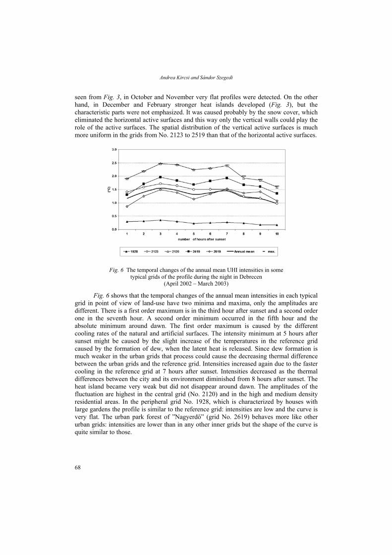
Andrea Kircsi and Sándor Szegedi
seen from Fig. 3, in October and November very flat profiles were detected. On the other hand, in December and February stronger heat islands developed (Fig. 3), but the characteristic parts were not emphasized. It was caused probably by the snow cover, which eliminated the horizontal active surfaces and this way only the vertical walls could play the role of the active surfaces. The spatial distribution of the vertical active surfaces is much more uniform in the grids from No. 2123 to 2519 than that of the horizontal active surfaces.
Fig. 6 The temporal changes of the annual mean UHI intensities in some
typical grids of the profile during the night in Debrecen (April 2002 – March 2003)
Fig. 6 shows that the temporal changes of the annual mean intensities in each typical grid in point of view of land-use have two minima and maxima, only the amplitudes are different. There is a first order maximum is in the third hour after sunset and a second order one in the seventh hour. A second order minimum occurred in the fifth hour and the absolute minimum around dawn. The first order maximum is caused by the different cooling rates of the natural and artificial surfaces. The intensity minimum at 5 hours after sunset might be caused by the slight increase of the temperatures in the reference grid caused by the formation of dew, when the latent heat is released. Since dew formation is much weaker in the urban grids that process could cause the decreasing thermal difference between the urban grids and the reference grid. Intensities increased again due to the faster cooling in the reference grid at 7 hours after sunset. Intensities decreased as the thermal differences between the city and its environment diminished from 8 hours after sunset. The heat island became very weak but did not disappear around dawn. The amplitudes of the fluctuation are highest in the central grid (No. 2120) and in the high and medium density residential areas. In the peripheral grid No. 1928, which is characterized by houses with large gardens the profile is similar to the reference grid: intensities are low and the curve is very flat. The urban park forest of ”Nagyerdő” (grid No. 2619) behaves more like other urban grids: intensities are lower than in any other inner grids but the shape of the curve is quite similar to those.
68

The development of the urban heat island studied on temperature profiles in Debrecen
CONCLUSIONS
• The profile is best developed between 3-6 hours after sunset. In that time the ”cliff”, the ”plateau” and the ”peak” appear. Later the “cliff” disappears and the ”slope” forms instead of the ”plateau”.
• The best profiles were found in the non-heating season, especially in August due to the prevailing anticyclonic weather conditions. In the heating season much weaker profiles were detected. In October, November and January rather flat profiles were found.
• There is a second order minimum of the intensities in the inner part of the city at 5 hours after sunset and a second order maximum at 7 hours after sunset. The second minimum is caused by the thermal excess in the reference grid due to the strong dew formation there, while the second intensity maximum can be interpreted as a consequence of the faster cooling outside the city in the second half of the night.
• The shape of the profile is quite similar in the inner parts of the city, even in the urban park forest, while in the outskirts the shape is rather flat.
Acknowledgements – This research was supported by the grant of the Hungarian Scientific Research Fund (OTKA T/034161). The work of the second author was also supported by the Bólyai János Scholarship of the Ministry of Education (BO/00047/02).
REFERENCES
Conrads, L.A. and van der Hage, J.C.H., 1971: A new method of air-temperature measurement in urban climatological studies. Atmos. Environ. 5, 629-635.
Oke, T.R., 1987: Boundary layer climates. Routledge, London - New York. Park, H-S., 1986: Features of the heat island in Seoul and its surrounding cities. Atmos. Environ. 20, 1859-1866. Unger, J., Bottyán, Z., Sümeghy, Z. and Gulyás, Á., 2000: Urban heat island development affected by urban
surface factors. Időjárás 104, 253-268. Unger, J., Sümeghy, Z. and Zoboki, J., 2001a: Temperature cross-section features in an urban area. Atmos. Res. 58,
117-127. Unger, J., Sümeghy, Z., Gulyás, Á., Bottyán, Z. and Mucsi, L., 2001b: Land-use and meteorological aspects of the
urban heat island. Meteorol. Applications 8, 189-194. Voogt, J.A. and Oke, T.R., 1997: Complete urban surface temperatures. J. Appl. Meteorol. 36, 1117-1132.
69


ACTA CLIMATOLOGICA ET CHOROLOGICA Universitatis Szegediensis, Tom. 36-37, 2003, 71-78.
LANDSCAPE EVALUATION ON SODIC LAND OF PÉLY AT HUNGARY (ECOTOPE-FORMING VALUE)
L. KÜRTI and I. BÁRÁNY-KEVEI
Department of Climatology and Landscape Ecology, University of Szeged, P.O.Box 653, 6701 Szeged, Hungary E-mail: [email protected]
Összefoglalás: A tanulmány egy német tájértékelési módszer felhasználásával értékeli egy magyar szikes táj ökotópképző értékét. Az értékelés alapját az adott területen megtalálható vegetáció adja. A vegetáció tulajdonképpen nem más, mint az abiotikus tényezők indikátora az ökoszisztémában. A biotikus és abiotikus tényezők együttesen alkotják a térben lehatárolt ökotópot. Az ökotóp a táj eltartóképességéről ad információt, mely bizonyos határig képes magát fenntartani és megújítani. A kapott eredmények az előzetes várakozásoknak megfeleltek, a táj ökotópképző értéke közepesnek minősíthető. Summary: In the landscape ecology there is several methods to evaluate the each landscape. This should be very important for other practical sciences like engineering and natural protecting. The study area is already protecting, but it needs rehabilitation.We used the method after a German landscape method. This method is based on the local vegetation, because the vegetation is the indicator of the abiotic factors in the eco-system. The ecotope is able to keep itself on a certain level and can regenerate itself. So it should be give us some information about the landscape-household system. The result, what we got, corresponds to our previous expectations; the ecotope forming value is average on the study area
Key words: landscape evaluation, ecotope, sodic land, plant association and communities
INTRODUCTION
Landscape ecology is an emerging science, with complex character and heterogeneous content, but with a clearly philosophical (epistemological) background (Zonneveld, 1990). It examines together the dynamic of spatial variegation of the earth- surface, the space and time-relation between the landscapes, it takes research on the influence of the spatial heterogeneity to the biotic and abiotic processes, and it is occupied in landscape planning (Risser et al., 1984). The aim of landscape ecology is to reveal the dynamic of energy and material flow in the eco-systems, to analyze the answers of eco-systems to the anthropogenic influences and know the indicators of these processes. To examine all of these factors together several methods were known.
One of the methods is to determine the ecotope-forming value. The ecotope-forming value gives information about the landscape-household capacity, which is good to know in the point of view of landscape using.
We used this method to evaluate grassland on the sodic lands of Pély. The base of the investigation was the local vegetation, because the plants are the indicators of the various conditions of landscape.
71

Lívia Kürti and Ilona Bárány-Kevei
The aim was to examine if the present landscape use is harmonious with the landscape-support capacity, and what kind of limiting and risky factors are in the present system. We also analyzed the alternative landscape using.
Previously the each abiotic factor was examined in the point of view the different landscape using: f.e. the soils were evaluated in old crown to show how it is valuable (Lóczy, 1989). At Hungary the first great complete landscape evaluation was made by Csorba P. in the basin of Bodrogkeresztúr in the end of the ’70 (Csorba, 1989).
The ecotope forming value was appeared in the Hungarian references just few years ago (Bárány-Kevei, 1997). The first, who used this method to evaluate Bárány-Kevei, who utilized it to evaluate the forests around Bodony. We also used the same method, but the characters of this area were different in our case.
METHODS AND STUDY AREA
The sodic land of Pély is situated on the northern part of the Great Hungarian Plain, on the middle-flood area of Tisza. Its development was determinate by the neighbourhood of Tisza until the human appearance (Fig. 1).
BUDAPEST
MISKOLC
EGER
Fig. 1 The situation of the study area in Hungary
Till 17th century the inhabitants have lived in a strong relation with their natural
environment: they used the grasslands for grazing between the marshes. With the growing of the local population they needed to cultivate more and more field. From this time more marshes were drained and dried up. There were two periods when these works have got a great impulse: the control of Tisza and the great canal-buildings in the 1950 years. The disappearance and degradation of various biotopes were the consequences of these processes. After than the landscape was appointed to the National Park, it was more important to restore the conditions natural or close to natural conditions. In the present day a mosaic landscape should be seen with many different plant associations (Fig. 2).
As the plant- associations give the base of the evaluation, so we had to need a vegetation map and the exact composition of species of each association (Marks et al., 1989). The National Park helped us in this work. We have found the following communities on the study area:
72

Landscape evaluation on sodic land of Pély at Hungary (ecotope-forming value)
1. Reeds (Scripo-Phragmitetum) (Koch, 1926) 2. Sodic field with foxtail grass (Argrosti-Alopecuratum pratensis) (Soó, 1947) 3. Sodic field with Beckmannia eruciformis (Agrostio-Beckmannietum) (Soó, 1933) 4. Sodic field with grass (Achilleo-Festucetum pseudovine) (Soó, 1945) 5. Sodic field with wormwood (Artemisio-Festucetum pseudovine) (Rapcs and Soó,
1947)
Key to signs
1 km
Achilleo-Festucetum
Artemisio- Festucetum
Artemisio- Festucetum with sodic seats
Agrostio- Alopecuretum pratensis
Agrostio-Beckmannietum
Alopecuretum
Scripo-Phragmitetum
Bolboschoenetum maritimi
Settlement
Fig. 2 The vegetation map of the study area
The ecotope-forming value, which expresses the productivity of the landscape, is
determinated by the potentials of landscape. But the conditions of landscape do not form ecotope by themselves. So the ecotope- forming value comes into being in the ecotope, which is determinated in space, through the effect system of biotic and abiotic components of landscape. The ecotope is able to regenerate and maintain itself till a certain level. The ecotopes constitute biotopes for the life assemblage of animals and plants (biocoenosis is formed by the species of animal and plants living together in symbiosis) (Bárány-Kevei, 1997).
The stable biotopes are able to keep or restore their equilibrium condition after a longer time, owing to their high stability and regenerator capacity.
The ecotope-forming value depends on the maturity, the naturalness, diversity and the anthropogenic influence of the community in a plant association. These components should be numericated by field work and mapping, inclusion. It is obvious that this
73

Lívia Kürti and Ilona Bárány-Kevei
procedure aims at the evaluation of the biotic components. But the values show the support capacity of the landscape, and at the same time they are the indicators of the change of conditions of the landscape.
Maturity of the communities
The maturity is the stage in the cyclical pattern of community stage in the plant succession. The succession development advances to the climax stage, which is the final stage, and the vegetation reaches a state of equilibrium with the environment. The succession is natural if the line of the stages is suited to the natural potentiality. The succession is secondary if it was formed by human impact. After the deforestation a secondary succession is formed. Unfortunately on most part of the study area we have found secondary vegetation, which is the consequence of the grazing during centuries and the drainage. The maturity should be measured on a scale from 1 to 5, and the initial stage got 1, while the climax stage got 5 (Table 1).
Table 1 The values of the maturity
Degree of the maturity Title
5 Climax community
4 Stable communities (they are stable with conditions external)
3 Long life additional comm. 2 Pioneer and short life add. comm. 1 Pioneer comm. In the initial stage
The naturalness of the plant association
The association is natural when it is up to the ecological conditions, it can regenerate easily answering to the perturbing impacts, elements. We determinate the naturalness with field work and category according to Simon, which means that we considered how high is than rate of the natural species in the community.
The naturalness should be measured on a scale from 0 to 5, and the association is closer to the most natural stage it get more points (Table 2).
Table 2 The classes of naturalness
Class of naturalness Nomination Value 1 Close to natural 5 2 Semi-natural 3 3 Far from natural 1 4 Artificial 0
The diversity of the community
The diversity means that the association is rich structurally and it has high number of species. Generally the ecosystems with high diversity are stable, which means that the
74

Landscape evaluation on sodic land of Pély at Hungary (ecotope-forming value)
energy- and material flux is well organized in the system. At the same time after a deep perturbation it regenerates more difficult, like in the simple organized systems. In normal case the climax-ecosystems have larger diversity then the pioneer or the following associations. We determinate the diversity with the species richness and structural diversity.
D = (G + S)/2
Where (D) is diversity, (G) is species richness and (S) is structural diversity.
As we wrote, as the larger number of the species grow the stability of the system, the structural diversity make to be stable the ecotope. This means that large structural variety gives larger point to the association. For example: if there is 40 or more species in the association, the D value will be 5, but if the number of the species 10 or less the D-value will be 1 (Table 3).
Table 3 The values of the richness of species
Number of species Value
> 40 5
31- 40 4
21- 30 3
11- 20 2
1 - 10 1
In the case of the structural diversity we examined what kind of percent the each structural unit has in the spatial structure of the community. We analyzed grassland in this research, we saw two structural unit, that means low-grass (lower than 30 cm) and high-grass unit (higher than 30 cm) appeared in this landscape (Table 4).
Table 4 The classification of the structural diversity
Height of vegetation units 50 – 100 % 25 – 50 % 5 – 25 % High wood (10-20 m) 1 0.6 0.3
Low wood (10 m alit) 1 0.6 0.3
Bush ( higher than 2 m) 1 0.6 0.3
Low bush (lower than 2 m) 0.5 0.3 0.2
Grass higher than 30 cm 1 0.6 0.3
Grass lower than 30 cm 0.5 0.3 0.2
Anthropogenic damage of the eco-system
The semi-natural and secondary plant associations and eco-systems answer with reduced productivity to the perturbation human activity (Table 5). The damage of the ecological condition should be the consequence of anthropogenic erosion, cultivation, drainage disordered, road buildings, irrigations, irregular depositions etc.
75

Lívia Kürti and Ilona Bárány-Kevei
Table 5 The classification of the anthropogenic influence
2 Under small influence 1 – 2 4 3 Influenced 2 – 5 3 4 Damaged 5 – 20 2 5 Very damaged 20 – 50 1 6 Very hard damaged Above 50 0
Description of evaluation
To simplify the procedure of valuation we ordered the values of the associations to the orders of the certain indicators. With this method we can save the field work of maturity and diversity and naturalness.
At determination of naturalness degree we considered how great the rate of the species referring to natural state was. (F.e protected species, pioneer species, and companion species) If the communities taking depart from the normality, than we must evaluate the order of indicators one by one. We must point out the anthropogenic damage in every case if we could not it determinate exactly.
We get the ecotope-forming value when we add together all values of the indicators:
EFV = M+N+D+A
Where: EFV-ecotope-forming value M-maturity N-naturalness D-diversity A-anthropogenic influence
This method can be used solely at the real species staff of ecosystem and plant association. The available highest value is 20, while the lowest is 1.5. Our results are in the Table 6.
Table 6 The Ecotope-forming values on the study area
Type of the community Maturity Naturalness Diversity Anthr.influence EFV
Reeds 3 5 1.65 4 13.65 Sod.f.w.foxt.grass 3 3 2.05 2 11.05
Sod.f.w.wormwood 4 3 2.05 3 12.05 Sod.f.w.Beckmannia 4 3 2.75 3 12.75
Sod.f.w.grass 3 3 2. 55 2 10.55
In the point of view of maturity there is no great variability on the study area. In the most case the associations are long life additional communities or natural succeeding communities. We have found higher level, lasting communities. These were the sodic meadows and wormwood sodic fields. We have not found association in climax stage, which means that there is no natural association on the study area. All association had significance anthropogenic influences. Especially, if we consider that there were several great marshes at the end of the 19th century.
76
Landscape evaluation on sodic land of Pély at Hungary (ecotope-forming value)
The value of diversity is very low. There are no associations rich in species and the structural diversity is neither variable. In fact this has two types in the area: low and high grass. The diversity is highest in case of sodic fields with Beckmannia eruciformis.
If we examine the naturalness, we have to establish that the natural following, or close to nature conditions are dominant, but the signs referring to degradation have been already appeared. The appearance of the reed indicates this phenomenon, and probably it is connected with the increase of the nitrogen loading.
All of the communities are influenced by anthropogenic activities. Their composition of species is disturbed which is well shown by the great number of the weeds. The anthropogenic influence is not only the grazing, but other agricultural, and not agricultural activities. For example the using of the ways besides the meadows should be the cause of the breaking up of the grass. But the protected area is enclosed by plough-lands, so their cultivation affects them. This means partly that the wed species spread.
On our study area the ecotope-forming value is between 10 and 14. The sodic field with foxtail grass, sodic field with grass, sodic field with wormwood have an average EFV. While the reeds and sodic fields with Beckmannia eruciformis got a high value.
These values correspond to our previous expectations. This means that the biotope developed here are relatively stables. The landscape-household capacity is not so high, and it is in a sensitive equilibrium with the present landscape using, because this is a cultivated (culture) landscape developed during centuries. The quantity of the biomass is not so much during a year, because of the low grass plant associations, and great part of them dries in the summer. In the autumn we can notice a secondary green shoot, but this has not great importance. Furthermore the yearly yield of grass depends on the climatic conditions of the given year too. This should be told all of the plant associations, but it is right especially in case of sodic lands, where extreme ecological conditions dominate. The local vegetation should be degradated if the landscape using does not correspond to the ecological conditions. Presently the study area is used as grazing land by sheeps and cows.
The National Park has begun rehabilitation. In this framework the old marsh would be restored as water–biotope, like in the 17th century. Probably in the close future the diversity is going to augment and the rate of the water- biotopes rises also, which should make changes in the local vegetation and fauna.
CONCLUSION
With regard to the study area, we can say that the sodic lands of Pély possess diverse ecotopes, but their landscape support capacity is average. The change in the natural conditions is the consequence of the human activities in the 15th century. For the moment the present ecotopes are in equilibrium with the landscape use, and as this is a protected area it should consider the viewpoint of the protection too during the usage.
In our opinion a regional, development plan is needed which support the sheep and cattle-farming with the possibility the processing, because Pély, the settlement is a poor, disadvantaged village. On the other hand to maintain these ecological conditions the area needs to be used as a grazing land.
We hope that the rehabilitation will be efficient, and the local water-biotopes will be more diverse than today, and the ecological conditions improve also.
77

Lívia Kürti and Ilona Bárány-Kevei
This analysis is based on the vegetation and hereby it takes the abiotic factors into consideration, because the vegetation communities are determinated by soil, climate, etc. As all ecological investigation, this is also based on a state survey temporary, so it would be advisable to repeat it certain intervals as a monitoring-system. As well as it is worth to compare other landscape evaluation methods.
This method needs some addition (other ecological indicators, or method) and also we should make more investigation to correct its insufficiency, or to propose a motion to specify the each factors.
REFERENCES
Bárány-Kevei, I., 1997: Az ökotópképző és természetvédelmi funkció meghatározása a Kataréti-patak vízgyűjtőjén (The determination of the ecotope-forming value and the natural protection value on the catchments area of the Kataréti stream). In Mezősi, G. and Rakonczai, J.: A geoökológiai térképezés elmélete és gyakorlata (The theory of geoecological plotting and its practice). Szeged, 57-71.
Csorba, P., 1989: Tájstabilitás és ökogegográfiai stabilitás (Landscape stability and ecogeographical stability). In Csorba, P. and Mezősi, G., 1995: Tájökológiai szöveggyűjtemény II. (The book of landscape ecology II.). Debrecen, 80-84.
Koch, W., 1926: Nádasok (Reeds). In Simon, T., 2000: A magyarországi edényes flóra határozója (Plant identification handbook of the Hungarian vascular plants). Nemzeti Tankönyvkiadó, Budapest, 758-759.
Lóczy, D., 1989: Tájökológiai elméletek, módszerek és gyakorlati alkalmazásaik (Theories and methods of landscape ecology and their practical applications). Földrajzi értesítő 38, 379-393.
Marks, R., Müller, M-J., Leser, H. and Klink, H.J., 1989: Anleitung zur Bewertung des Leistungsvermögens des Landschaftshaushaltes. Zentralausschuß für deutsche Landeskunde, Selbstverlag, Trier.
Rapcs and Soó, R., 1947: Ürmös szikes puszta (Sodic field with wormwood). In Simon, T., 2000: A magyarországi edényes flóra határozója (Plant identification handbook of the Hungarian vascular plants). Nemzeti Tankönyvkiadó, Budapest, 507-509.
Risser, P., Karr, J.K and Forman, R.T.T., 1984: Landscape ecology-directions and approaches. Nat. History Survey Spec. Publ. 2.
Soó, R., 1933: Hernyópázsitos szikirét (Sodic field with Beckmannia eruciformis). In Simon, T., 2000: A magyarországi edényes flóra határozója (Plant identification handbook of the Hungarian vascular plants). Nemzeti Tankönyvkiadó, Budapest, 768.
Soó, R., 1945: Füves szikes puszta (Sodic field with grass). In Simon, T., 2000: A magyarországi edényes flóra határozója (Plant identification handbook of the Hungarian vascular plants). Nemzeti Tankönyvkiadó, Budapest, 758-759.
Soó, R., 1947: Ecsetpázsitos szikirét (Sodic field with foxtail grass). In Simon, T., 2000: A magyarországi edényes flóra határozója (Plant identification handbook of the Hungarian vascular plants). Nemzeti Tankönyvkiadó, Budapest, 768-769.
Zonneveld, I.S., 1994: Scope and concepts of landscape ecology as an emerging science. In Mezősi, G. and Csorba, P., 1994: Tájökológiai szöveggyűjtemény I. (The book of landscape ecology I.). Debrecen, 11-19.
78
ACTA CLIMATOLOGICA ET CHOROLOGICA Universitatis Szegediensis, Tom. 36-37, 2003, 79-83.
CONNECTION BETWEEN PHENOLOGICAL PHASES AND URBAN HEAT ISLAND IN DEBRECEN AND SZEGED, HUNGARY
L. LAKATOS1 and Á. GULYÁS2
1Centre of Agronomy, University of Debrecen, P.O.Box 36, 4015 Debrecen, Hungary E-mail: [email protected]
2Department of Climatology and Landscape Ecology, University of Szeged, P.O.Box 653, 6701 Szeged, Hungary
Összefoglalás – A városi környezetben jelentősen eltérő a felszín anyaga, szerkezete és ezekből adódóan az energiamérlege a természetes felszínekhez képest. E tényezők lokális klímamódosulást okoznak, melynek egyik sokat vizsgált jelensége a városi hősziget. Feltételezzük, hogy e módosulások a városban élő növényzet fenológiai, fenometriai mutatóira is hatással vannak. Két magyarországi város (Debrecen és Szeged) esetén végeztünk hőmérsékleti méréseket és fenológiai megfigyeléseket 2003 tavaszán. A napi megfigyelésekhez az aranyvesszőt (Forsythia suspensa) választottuk, mivel elterjedése 60-70%-os lefedettséget mutat mindkét város esetén. Eredményeink szerint a fenológiai fázisok bekövetkezési időpontjának területi adatai szignifikáns kapcsolatot mutatnak a hősziget intenzitás területi eloszlásával. Legszorosabb kapcsolatot a 100%-os virágzás bekövetkezési időpontja között találtunk, Debrecenben (0,1%-os szinten szignifikáns). Summary – A local climate with special spatial structure (e.g. heat island) is formed within the settlement compared to outside open spaces. We presume that these climatic modification affects the phenological and phenometrical properties of the urban vegetation. For this study we have chosen two medium-sized Hungarian cities (Szeged and Debrecen), with urban areas over 30 km2 and with population between 160 and 200 thousand. The phenological and temperature observations have been taken in grid networks in spring of 2003. As a good observable plant, forsythia (Forsythia suspensa) was the object of our examination because this species occurs in the 60-70% of the areas of both cities. The time of the different phenological phases was monitored in a daily fashion. According to the results there is significant correlation between the spatial distributions of the timing of these phenological phases and of the intensity of the urban heat island. The strongest correlation occurs between the UHI intensity and the date of 100% flowering in Debrecen.
Key words: phenology, urban heat island, Forsythia suspensa, Debrecen, Szeged, Hungary
INTRODUCTION
Phenological observations were used as a bioindicative method by ecological research and the applied agricultural practice for a long time (Fezer, 1995; Schwartz, 1999). Impact of global climatic change on vegetation was widely investigated using long-term data and remote sensing (Defila and Clot, 2001; Valentini et. al., 2001). Other researches studied the small scale modifying effect of urban climate on urban vegetation (e.g. Roetzer et. al., 2000). The city itself represents a modified ecological environment for plants in many aspects (urban heat island phenomenon, high building density, air pollution, soil sealing and pollution, water balance) so pattern of phenological data represents mainly an ecological-microclimatical stuctures of urban area (Karsten, 1986). The results of these researches indicate that flowering of different plant species happened earlier in urbanised
79

László Lakatos and Ágnes Gulyás
than in rural areas (Roetzer et al., 2000). So shift of phenological phases is a result of a complex mechanism but it can be linked to the urban heat island (UHI) intensity.
The objective of this study is to analyse the eco-climatic effects in two Hungarian middle-sized cities, Debrecen and Szeged.
STUDY AREA AND METHODS
The investigated areas, Debrecen (47.5ºN, 21.5ºE) and Szeged (46ºN, 20ºE) are located in the north-eastern and in the south-eastern part of Hungary at 120 m and 79 m above sea level, respectively, on a flat plain. Administration districts of Debrecen (220,000 inhabitants) and Szeged (160,000 inhabitants) are about 300 km2 (Fig. 1). Debrecen does not have any larger river, while River Tisza passes through Szeged. Szeged has a boulevard-avenue road system structure with a heavily built up centre region and housing estate zone in north-eastern part of the city. Debrecen has a less centre region at about the geometrical centre of the city than Szeged but there is a huge housing estate zone in the western part of the city. We used for the observation a 500 x 500 m grid network which was applied earlier for urban climate research (Unger et al., 2001). Having averaged the phenological data the received mean values refer to the centre of each cell.
The investigated species was forsythia (Forsythia suspensa), because its distribution is well extended (60-70%) over both cities. The times of four selected phenological phases (beginning of the flowering, 25%, 50% and 100% blooming) of the plants (4-8 in one grid cell) were recorded. Blooming maps show the day’s numbers starting from the 1st of January 2003 (year day – YD), similar to Steinecke (1999). In order to assess the extent of the relationships between the mean maximum UHI intensity and blooming events, correlation and regression analyses were applied in the statistical data processing.
200 km0 100
A
B D
C
Fig. 1 Geographical location of Hungary in Europe (A), of Debrecen and Szeged in Hungary (B), and the measurement grid networks in Debrecen (C) and in Szeged (D). The urbanized areas are marked
by grey on the parts of C and D.
80

Connection between phenological phases and urban heat island in Debrecen and Szeged, Hungary
RESULTS AND DISCUSSION
The urban climatological investigations in Szeged (UHI, humidity, human comfort) have a tradition of several years (e.g. Unger, 1992, 1999a, 1999b). Recent urban climate studies show maximum urban heat island intensities of 2.3ºC in Debrecen (Fig. 2A) and 2.7ºC in Szeged (Fig. 2B) as annual averages between April 2002 and March 2003. These values can extend up to 5.8ºC and 6.8ºC in Debrecen and in Szeged, respectively, at clear, anticyclonic weather conditions (Szegedi and Kircsi, 2003; Sümeghy and Unger, 2003). In our study the maximum UHI is the urban-rural temperature difference a few hours after sunset, when the UHI effect is most pronounced in its daily course.
A
0.5 1.0
B
Fig. 2 Spatial distribution of the mean maximum UHI intensity (April 2002 – March 2003) in Debrecen (A) and Szeged (B)
A
B
Fig. 3 Spatial distribution of the beginning (in YD) of the blooming Forsythia suspensa in Debrecen (A) and in Szeged (B) in spring 2003
Based on the received data, in both cities pheno-isochrone maps on spatial
distribution of the different flowering dates were created. According to the results there is significant connection between the spatial distribution of the phenological data and of the heat island intensity. Two examples are presented to support this statement: Fig. 3 and Fig. 4 show the spatial distribution of the beginning of flowering and the full-flowering phenophases, respectively (A – Debrecen, B – Szeged). We have to mention, that the observation in
81

László Lakatos and Ágnes Gulyás
Debrecen covered more clusters, hence maps refer to Debrecen have higher resolution than those which regard to Szeged. As the figures show the investigated plants reached the given phase earliest time in the heavily built-up centre and housing estate region. These regions represent the highest UHI intensity, too (Fig. 2). Shapes of isolines are stretching out towards W in Debrecen and towards N-NE in Szeged due to the urban structure.
On account of macrosynoptical conditions and geographical location the flowering began in Debrecen 2-4 days after Szeged and the blooming process was drawling. The full-flowering phase occurred 10 days later than in Szeged.
A
B
Fig. 4 Spatial distribution of the date (in YD) of the full-flowering phenophases of Forsythia suspensa in Debrecen (A) and Szeged (B) in spring of 2003
Fig. 5 shows the
correlation between UHI intensity and date of 100% flowering in Debrecen in spring of 2003 by cells. The correlation coefficient is r = -0.6473 (r2 = 0.4109) with a standard deviation of 2-3 days. It means that in such a complex modified process like blooming a
relationship at a significance level of 0.1%. As the regression line presents the relationship between the two variables is negative, as it was expected.
strong
y = -1.4456x + 114.36
R2 = 0.4109
95
100
105
110
115
120
-1 0 1 2 3 4 5 6
Urban heat island intensity (°C)
Date
of t
he f
ull-f
lower
ing
phas
es
from
1st
of J
anua
ry
Fig. 5 Correlation between the urban heat island intensity and the date (in YD) of the full-flowering phenological
phases in Debrecen in spring 2003
CONCLUSIONS
The following conclusions are reached from the analysis presented: (i) Pattern of phenological phases shows good correlation with microclimatological
data.
82

Connection between phenological phases and urban heat island in Debrecen and Szeged, Hungary
(ii) Significant differences were experienced in the blooming date between city centres and suburbs in both cities.
(iii) Phenological phases can be shifted earlier by several days even one week (in our investigation 4-8 days) in heavily built city centre region and blocks-of-flats areas with high intensity heat island.
(iv) Time shifting of phenological phases can be attributed partly to the effect of urban heat island.
(v) The geographical location and the macrosynoptical conditions caused differences in blooming date between the two experienced cities.
Acknowledgements – This research was supported by the grant of the Hungarian Scientific Research Fund (OTKA T/034161). The figures were drawn by Z. Sümeghy.
REFERENCES
Defila, C. and Clot, B., 2001: Phytophenological trends in Switzerland. Int. J. Biometeorol. 45, 203-207. Fezer, F., 1995: Das Klima der Städte. Justus Perthes Verlag, Gotha, 199 pp. Karsten, M., 1986: Eine Analyse der phaenologischen Methode in der Stadtklimatologie am Beispiel der
Kartierung Mannheims. Selbstverlag des Geographischen Institutes der Universität Heidelberg, Heft 84, Heidelberg.
Roetzer, T., Wittenzeller, M., Haeckel, H. and Nekovar, J., 2000: Phenology in central Europe - differences and trends of spring phenophases in urban and rural areas. Int. J. Biometeorol. 44, 60-66.
Schwartz, M.D., 1999: Advancing to full bloom: planning phenological research for the 21st century. Int. J. Biometeorol. 42, 113-118.
Steinecke, K., 1999: Urban climatological studies in the Reykjavík subarctic environment, Iceland. Atmos. Environ. 33, 4157-4162.
Sümeghy, Z. and Unger, J., 2003: Classification of the urban heat island patterns. Acta Climatologica et Chorologica Universitatis Szegediensis 36-37 (this issue), 93-100.
Szegedi, S. and Kircsi, A., 2003: The effects of the synoptic conditions on development of the urban heat island in Debrecen, Hungary. Acta Climatologica et Chorologica Universitatis Szegediensis 36-37 (this issue), 111-120.
Unger, J., 1992: Diurnal and annual variation of the urban temperature surplus in Szeged, Hungary. Időjárás 96, 235-244.
Unger, J., 1999a: Comparisons of urban and rural bioclimatological conditions in the case of a Central-European city. Int. J. Biometeorol. 43, 139-144.
Unger, J., 1999b: Urban-rural air humidity differences in Szeged, Hungary. Int. J. Climatol. 19, 1509-1515. Unger, J., Sümeghy, Z., Gulyás, A., Bottyán, Z. and Mucsi, L., 2001: Land-use and meteorological aspects of the
urban heat island. Meteorol. Applications 8, 189-194. Valentini, N., Me, G., Ferrero, R. and Spanna, F., 2001: Use of bioclimatic indices to characterize phenological
phases of apple varieties in Northern Italy. Int. J. Biometeorol. 45, 191-195.
83


ACTA CLIMATOLOGICA ET CHOROLOGICA Universitatis Szegediensis, Tom. 36-37, 2003, 85-93.
EVALUATION OF THE AIR QUALITY OF SZEGED WITH SOME ASSESSMENT METHODS
L. MAKRA1, H. MAYER2, R. BÉCZI1 and E. BORSOS1
1Department of Climatology and Landscape Ecology, University of Szeged, P.O.Box 653, H-6701 Szeged, Hungary, E-mail: [email protected]
2Meteorological Institute, University of Freiburg, D-79085 Freiburg, Germany
Összefoglalás – A légkör emberre gyakorolt hatásainak becsléséhez a humán biometeorológia módszereit kell alkalmazni. A humán biometeorológia összetevői közül a termikus komponens, valamint a levegőminőségi komponens játssza a legfontosabb szerepet. A légszennyező anyagok koncentrációinak vizsgálatához szükséges küszöbértékeik mindenütt rendelkezésre állnak. A levegőminőségi komponens értékelése céljából egyrészt statisztikai alapú ún. levegőterhelési indexeket, másrészt hatás alapú ún. levegőminőségi indexeket fejlesztettek ki. A dolgozatban egy Szeged-belvárosi forgalmi csomópontban működő monitoring állomás ötéves 30 percenkénti adatbázisa alapján összehasonlítottuk a statisztikai alapú ASISz levegőterhelési index, valamint egy újonann előállított hatás alapú levegőminőségi index (DAQx) értékeinek gyakorisági eloszlásait. Mindkét indexet német kutatók fejlesztették ki, s napi adatbázis alapján számíthatók. A két index gyakorisági eloszlás görbéinek eltérő alakja az egyes légszennyező anyagok hatás alapú koncentrációinak megadott tartományaira vezethető vissza, melyek a levegőminőségi indexek jellmezői. Az adatbázis alapján a levegőminőségi indexek értékeiben elsősorban a szén-monoxid és a PM10 részesedése számottevő. Summary – Methods of human-biometeorology have to be applied for the assessment of atmospheric impacts on human beings. Among the human-biometeorological effective complexes two are of great importance in the regional scale: the thermal effective complex and the air quality effective complex. With respect to the air quality effective complex, standards for the assessment of single air pollutants exist worldwide. In addition, approaches for statistical air stress indices and impact-related air quality indices were developed. In this study, based on a five-year air pollutant data set from the downtown of a middle-sized Hungarian city, Szeged, the frequency distribution of the air stress index ASISz is compared with the frequency distribution of the new air quality index DAQx. Both indices were developed by German researchers and are on a daily basis. The varying forms of both frequency distributions are mainly caused by the impact-related concentration ranges of single air pollutants, which are typical of air quality indices. Especially carbon-monoxide and PM10 have a stronger influence on the determination of values of air quality indices.
Key words: air pollution, air stress index (ASI), air quality index (DAQx)
INTRODUCTION
There are a lot of questions on the impacts of the atmospheric environment on human beings which are focussed on the regional scale (e.g. landscape planning). To get answers, methods of human-biometeorology have to be applied (Mayer, 1993). Among the human biometeorological effective complexes two are of great importance in the regional scale: the thermal effective complex (Matzarakis and Mayer, 1997; Matzarakis et al., 1999; 2000) and the air quality effective complex (Mayer et al., 2002a, 2002b). They have to be assessed in a human biometeorologically significant manner. Assessment of air quality
85

László Makra, Helmut Mayer, Rita Béczi and Emőke Borsos
developed only a few studies in Hungary (e.g. Makra and Horváth, 2001). The objective of this article is twofold: on the one hand, to give a brief overview of assessment methods; and, on the other hand, to discuss exemplary results for air pollution data basis of Szeged.
METHODS
Standards for the assessment of single air pollutants exist in almost every country of the world, e.g. in EU directives. However, these standards are insufficient in view of the persistent demands (e.g. from planners) for the assessment of the air quality, which is not limited to a single air pollutant. Therefore, indices on the basis of routinely monitored air pollutants were developed. They can be categorized into two groups (Mayer et al., 2002b). The first group includes indices, which are only statistical and have no direct relation to the well-being and health of human beings. They indicate mainly the content of air pollution in the ambient air and, therefore, are called air stress indices ASI. They can be calculated according to the following formulas:
i
n
i i
iRC
nASI ∑
=
=
1*1 (1)
with a symbol description in Table 1.
Table 1 Description of the air stress index ASI in formula (1)
mean stress (year, day) short-term stress n number of air pollutants number of air pollutants
C time specific concentration
of the air pollutant i number of cases per calendar year: air
pollutant specific limit values are exceeded
R
time specific reference (limit) value of the air pollutant i
number of cases per calendar year: air pollutant specific limit values are not to be
exceeded
Planning-related air stress index ASI1 for mean stress, developed by the Office of Environmental Protection, Division Urban Climate, City of Stuttgart, Germany:
+++= 33
103
23
21
/5)(
/40)(
/40)(
/20)(*
41
mgbenzeneC
mgPMC
mgNOC
mgSOC
µµµµASI (2)
where C: arithmetical annual mean values (µg/m3); reference values (denominators of the addable sums): air pollutant specific EU standards.
Planning-related air stress index ASI2 for short-term stress, developed by the Office of Environmental Protection, Division Urban Climate, City of Stuttgart, Germany:
+++=1
)(35
)(18
)(24
)(*41 1022
2CONPMNNONSONASI (3)
86

Evaluation of the air quality of Szeged with some assessment methods
where N: number of cases per calendar year, air pollutant specific EU limit values are exceeded; reference values (denominators of the addable sums): number of cases per calendar year, air pollutant specific EU limit values are not to be exceeded [SO2: 350 µg/m3 (1 h mean value), NO2: 200 µg/m3 (1 h mean value), PM10: 50 µg/m3 (daily mean value), CO: 10 mg/m3 (highest daily running 8 h mean value)] (Mayer et al., 2002b).
A graded assessment scale (Table 2) is available for the air stress indices ASI1 and ASI2 (Mayer et al., 2002b), which e.g. can serve as basis for planning specific recommendations with respect to the air quality.
Table 2 Assessment of the air quality conditions on the basis of ASI1 and ASI2 (Mayer et al., 2002b)
ASI1: no single air pollutant exceeds the corresponding limit value ASI2: no single air pollutant shows a higher number of cases per calendar year with air pollutant specific limit values are exceeded than the permitted number level I very low air stress ASI1, ASI2 < 0.2 level II low air stress 0.2 ≤ ASI1, ASI2 < 0.4 level III moderate air stress 0.4 ≤ ASI1, ASI2 < 0.6 level IV distinct air stress 0.6 ≤ ASI1, ASI2 < 0.8 level V strong air stress ASI1, ASI2 ≥ 0.8 ASI1: no less than one air pollutant exceeds the corresponding limit value ASI2: no less than one air pollutant shows a higher number of cases per calendar year with air pollutant specific limit values are exceeded than the permitted number level VI extreme air stress independent of ASI1 and ASI2
Air stress index ASISz on a daily basis, developed by the Federal State Institute for
Environmental Protection Baden-Wuerttemberg, Karlsruhe, Germany:
310
33
32
332
/50)(
/180)(
/200)(
/10)(
/350)(
mgPMC
mgOC
mgNOC
mmgCOC
mgSOC
Szµµµµ
++++=ASI (4)
Lower index Sz indicates data sets of Szeged city, to which this air stress index is applied). C(SO2), C(NO2), and C(O3): highest daily 1 h mean values (µg/m3), C(CO): highest daily running 8 h mean value (mg/m3), C(PM10): daily mean value (µg/m3); limit values from EU directives.
ASISz classes and ranges are as follows: I: ASISz < 0.5; II: 0.5 ≤ ASISz < 1.1; III: 1.1 ≤ ASISz <1.7; IV: 1.7 ≤ ASISz < 2.3; V: 2.3 ≤ASISz < 2.9; VI: ASISz ≥ 2.9.
Impact-related indices, which are called air quality indices, constitute the second group of indices for the assessment of the air quality effective complex. Such indices are very rare, because it is difficult to quantify the impacts of air pollutants on the well-being and health of human beings. The methodology of air quality indices is to assign concentrations of ambient air pollutants to different air pollutant specific ranges. The air quality index itself is represented by the highest index class among the considered air pollutants. The relation to the impact on human beings is given by different classified ranges of air pollutant concentrations, which are derived from epidemiological and toxicological investigations.
A new impact-related air quality index obtained on a daily basis and abbreviated as DAQx (Daily Air Quality Index) was recently developed and tested by the Meteorological
87

László Makra, Helmut Mayer, Rita Béczi and Emőke Borsos
Institute, University of Freiburg, and the Research and Advisory Institute for Hazardous Substances, Freiburg, Germany (Mayer et al., 2002a, 2002b). DAQx considers the air pollutants SO2, CO, NO2, O3, and PM10. To enable a linear interpolation between index classes, DAQx is calculated for each air pollutant by
lowlowinstlowup
lowup DAQxCCCCDAQxDAQx
DAQx +
−
−
−= )(* (5)
with Cinst.: highest daily 1 h concentration of SO2, NO2, and O3, highest daily running 8 h mean concentration of CO, and mean daily concentration of PM10; Cup: upper threshold of specific air pollutant concentration range (Table 3); Clow: lower threshold of specific air pollutant concentration range (Table 3); DAQxup: index value according to Cup (Table 3); DAQxlow: index value according to Clow (Table 3).
Table 3 Assignment of ranges of specific air pollutant concentrations to DAQx values and DAQx classes inclusive of classification names according to school marks (Mayer et al., 2002a, b)
SO2 (µg/m³)
CO (mg/m³)
NO2 (µg/m³)
O3 (µg/m³)
PM10 (µg/m³)
DAQx value
DAQxclass
Classification
0– 24 0.0– 0.9 0– 24 0– 32 0.0– 9.9 0.5–1.4 1 very good 25– 49 1.0– 1.9 25– 49 33– 64 10.0–19.9 1.5–2.4 2 good 50–119 2.0– 3.9 50– 99 65–119 20.0–34.9 2.5–3.4 3 satisfactory 120–349 4.0– 9.9 100–199 120–179 35.0–49.9 3.5–4.4 4 sufficient 350–999 10.0–29.9 200–499 180–239 50.0–99.9 4.5–5.4 5 poor ≥ 1000 ≥ 30.0 ≥ 500 ≥ 240 ≥ 100 ≥ 5.5 6 very poor
DATA BASIS
The data basis of the study is formed by 30-minute air pollutants concentrations (SO2, NO2, CO, O3, PM10) of the monitoring station in the downtown of Szeged, for the five-year period between 1997-2001. The considered pollutants and the existing concentration data in percentage are shown in Table 4.
Table 4 Existing data for calculation of ASI1 and ASI2, %
Year 1SO2 1NO2 2PM10 3PM10 4CO 1997 6.11 67.24 85.56 83.56 90.14 1998 78.38 89.01 73.20 73.15 88.49 1999 99.81 95.53 72.76 72.60 99.18 2000 98.90 89.34 99.01 98.08 98.36 2001 98.65 98.95 96.36 95.07 98.08
11 h mean values; used for calculation of ASI1 and ASI2; 21 h mean values; used for calculation of ASI1; 3daily mean values; used for calculation of ASI2. It was calculated if at least 20 one-hour mean was at disposal on a
given day; 4highest daily running 8 h mean value. It was calculated if at least 20 one-hour mean was at disposal on a given day.
88
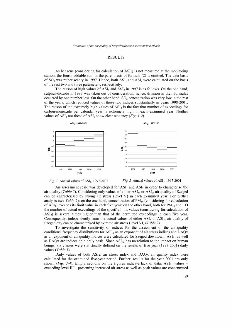
Evaluation of the air quality of Szeged with some assessment methods
RESULTS
As benzene (considering for calculation of ASI1) is not measured at the monitoring
station, the fourth addable sum in the parenthesis of formula (2) is omitted. The data basis of SO2 was rather scanty in 1997. Hence, both ASI1 and ASI2 were calculated on the basis of the rest two and three parameters, respectively.
The reason of high values of ASI1 and ASI2 in 1997 is as follows. On the one hand, sulphur-dioxide in 1997 was taken out of consideration; hence, division in their formulas occurred by one number less. On the other hand, SO2 concentration was very low in the rest of the years, which reduced values of these two indices substantially in years 1998-2001. The reason of the extremely high values of ASI2 is the fact that number of exceedings for carbon-monoxide per calendar year is extremely high in each examined year. Neither values of ASI1 nor those of ASI2 show clear tendency (Fig. 1-2).
ASI1, 1997-2001
0,0
0,2
0,4
0,6
0,8
1,0
1,2
1,4
1997 1998 1999 2000 2001
year
ASI
1
Fig. 1 Annual values of ASI1, 1997-2001
ASI2, 1997-2001
0
5
10
15
20
25
30
35
40
45
1997 1998 1999 2000 2001
year
ASI
2
Fig. 2 Annual values of ASI2, 1997-2001
An assessment scale was developed for ASI1 and ASI2 in order to characterise the air quality (Table 2). Considering only values of either ASI1, or ASI2, air quality of Szeged can be characterised by strong air stress (level V) in each examined year. For further analysis (see Table 2): on the one hand, concentration of PM10 (considering for calculation of ASI1) exceeds its limit value in each five year; on the other hand, both for PM10 and CO the number of actual exceedings of the specific limit values (considering for calculation of ASI2) is several times higher than that of the permitted exceedings in each five year. Consequently, independently from the actual values of either ASI1 or ASI2, air quality of Szeged city can be characterised by extreme air stress (level VI) (Table 2).
To investigate the sensitivity of indices for the assessment of the air quality conditions, frequency distributions for ASISz as an exponent of air stress indices and DAQx as an exponent of air quality indices were calculated for Szeged downtown. ASISz as well as DAQx are indices on a daily basis. Since ASISz has no relation to the impact on human beings, six classes were statistically defined on the results of five-year (1997-2001) daily values (Table 3).
Daily values of both ASISz air stress index and DAQx air quality index were calculated for the examined five-year period. Further, results for the year 2001 are only shown (Fig. 3-4). Empty sections on the figures indicate lack of data. ASISz values – exceeding level III – presenting increased air stress as well as peak values are concentrated
89

László Makra, Helmut Mayer, Rita Béczi and Emőke Borsos
in the winter half-year or in the winter months (Fig. 3). This can be explained by climatic reasons. Standard deviation of DAQx values is less than that of ASISz values. Peak values of DAQx are also concentrated in the winter half-year (Fig. 4); however, this is not as characteristic as in the case of ASISz values. The reason of this is that the vertical axis of the diagram for ASISz is linear, while that of the diagram for DAQx is not.
ASISz, 2001
0
1
2
3
4
5
6
7
8
0 30 60 90 120
150
180
210
240
270
300
330
360
day
ASI
Sz
Fig. 3 Annual course of ASISz, 1997-2001
DAQx, 2001
0
1
2
3
4
5
6
7
0 30 60 90 120
150
180
210
240
270
300
330
360
day
DA
Qx
Fig. 4 Annual course of DAQx, 1997-2001
Frequency distribution of ASISz and DAQx according to both classes and years are different. DAQx values have generally well higher frequencies in levels 4 and 5; and, on the other hand, have less ones in the rest levels comparing to frequency distribution of ASISz values in levels I-VI (Fig. 5-6).
ASISz - according to classes, 1997-2001
0
10
20
30
40
I II III IV V VI
ASISz - classes
freq
uenc
y, %
1997 1998 19992000 2001
Fig. 5a Frequency distribution of ASISz values
according to classes, 1997-2001
ASISz - according to years, 1997-2001
0
10
20
30
40
1997 1998 1999 2000 2001
year
freq
uenc
y, %
I II III IV V VI
Fig. 5b Frequency distribution of ASISz values
according to years, 1997-2001
Carbon-monoxide and PM10 are mainly responsible for the changed form of the frequencies of DAQx classes (Fig. 7).
There were selected those 3 days in each July and January in the examined five-year period, on which air pressure was the highest in the month. Afterwards, ASISz and DAQx values of these days were calculated. In July values of ASISz share of PM10, ozone and carbon-monoxide are the largest, while its January values are mostly determined by concentrations of CO and PM10 (Fig. 8a, c). When calculating DAQx values in July, highest index categories are shown by PM10 on 10 days, by O3 on 3 days and by CO on
90
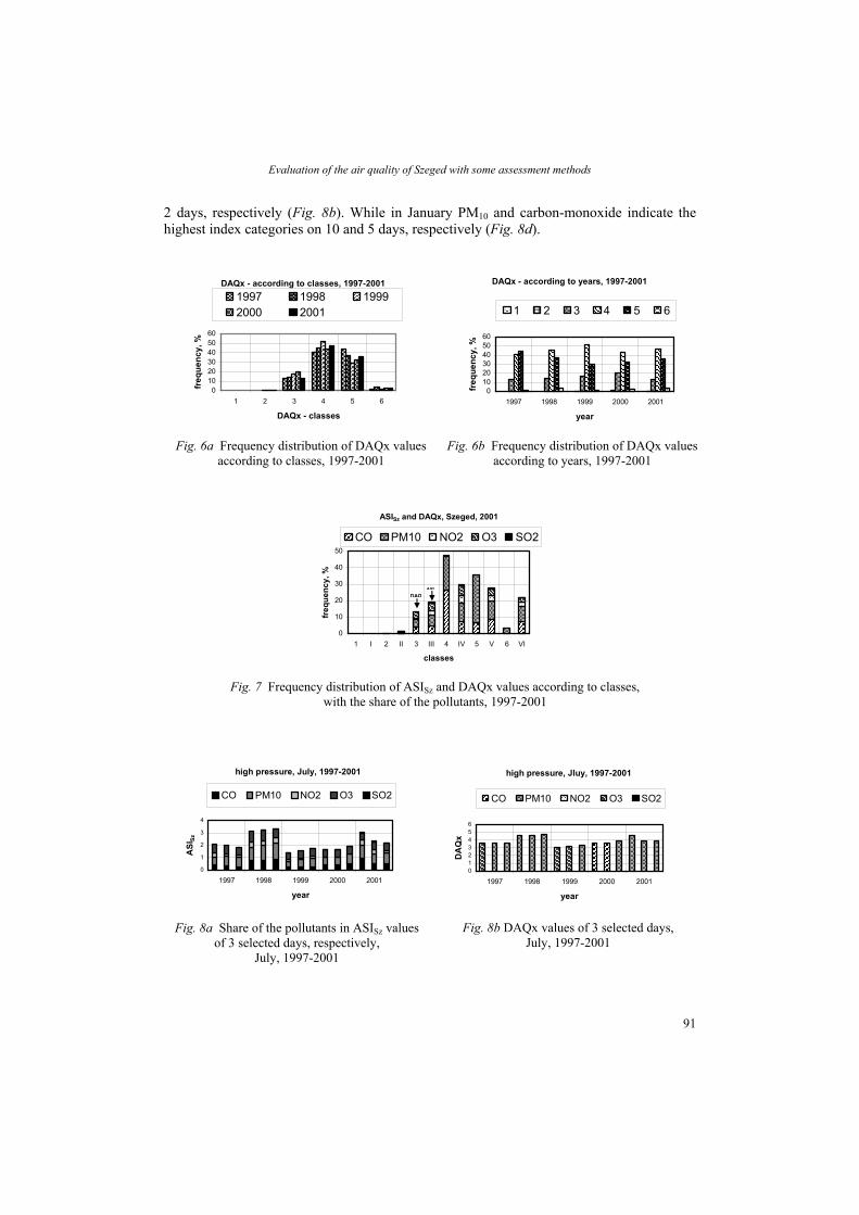
Evaluation of the air quality of Szeged with some assessment methods
2 days, respectively (Fig. 8b). While in January PM10 and carbon-monoxide indicate the highest index categories on 10 and 5 days, respectively (Fig. 8d).
DAQx - according to classes, 1997-2001
0102030405060
1 2 3 4 5 6
DAQx - classes
freq
uenc
y, %
1997 1998 19992000 2001
Fig. 6a Frequency distribution of DAQx values
according to classes, 1997-2001
DAQx - according to years, 1997-2001
0102030405060
1997 1998 1999 2000 2001
year
freq
uenc
y, %
1 2 3 4 5 6
Fig. 6b Frequency distribution of DAQx values
according to years, 1997-2001
ASISz and DAQx, Szeged, 2001
0
10
20
30
40
50
1 I 2 II 3 III 4 IV 5 V 6 VI
classes
freq
uenc
y, %
CO PM10 NO2 O3 SO2
ASIDAQ
Fig. 7 Frequency distribution of ASISz and DAQx values according to classes,
with the share of the pollutants, 1997-2001
high pressure, July, 1997-2001
0
1
2
3
4
1997 1998 1999 2000 2001
year
ASI
Sz
CO PM10 NO2 O3 SO2
Fig. 8a Share of the pollutants in ASISz values
of 3 selected days, respectively, July, 1997-2001
high pressure, Jluy, 1997-2001
0123456
1997 1998 1999 2000 2001
year
DA
Qx
CO PM10 NO2 O3 SO2
Fig. 8b DAQx values of 3 selected days,
July, 1997-2001
91

László Makra, Helmut Mayer, Rita Béczi and Emőke Borsos
high pressure, January, 1997-2001
0
1
2
3
4
1997 1998 1999 2000 2001
year
ASI
Sz
CO PM10 NO2 O3 SO2
Fig. 8c Share of the pollutants in ASISz values of 3 selected days, respectively,
January, 1997-2001
high pressure, January, 1997-2001
0123456
1997 1998 1999 2000 2001
year
DA
Qx
CO PM10 NO2 O3 SO2
Fig. 8d DAQx values of 3 selected days,
January, 1997-2001
Analysis of both ASISz and DAQx values represents high pollution load of PM10 and
carbon-monoxide. Examined parameters of PM10 and CO – which are several times higher than standards of their EU directives – substantially modifiy air quality of Szeged.
CONCLUSIONS
Aside from single air pollutant standards, air stress indices and air quality indices enable an additional assessment of the air quality conditions, which is primarily not limited to single air pollutants. The application of air stress indices or air quality indices depends on the specific objectives of the investigation.
Temporal course of ASI1 and ASI2 is not clear. High values of mean air stress (indicated by ASI1 ≈ 1) as well as extremely high values of short-term air stress (indicated by ASI2 > 20) suppose high air pollution load in Szeged.
Acknowledgement - The authors thank Gábor Motika (Environmental Protection Inspectorate of Lower-Tisza Region, Szeged, Hungary) for handing monitoring data of the air pollutants and meteorological elements to our disposal and Szilvia Horváth (Department of Climatology and Landscape Ecology, University of Szeged, Hungary) for valuable contribution.
REFERENCES
Makra, L. and Horváth, Sz., 2001: Assessment of air pollution in Szeged (in Hungarian). Légkör 46, 14-18. Matzarakis, A. and Mayer, H., 1997: Heat stress in Greece. Int. J. Biometeorol. 41, 34-39. Matzarakis, A., Mayer, H., and Iziomon, M.G., 1999: Applications of a universal thermal index: physiological
equivalent temperature, Int. J. of Biometeorol. 43, 76-84. Matzarakis, A., Rutz, F., and Mayer, H., 2000: Estimation and calculation of the mean radiant temperature within
urban structures. WCASP-50, WMO/TD, No. 1026, 273-278. Mayer, H., 1993: Urban bioclimatology, Experientia 49, 957-963. Mayer, H., Kalberlah, F., and Ahrens, D., 2002a: TLQ – Am impact related air quality index obtained on a daily
basis. Proceedings of the Fourth Symposium on the Urban Environment, Norfolk, VA (USA), 80-81. Mayer, H., Kalberlah, F., Ahrens, D., and Reuter, U., 2002b: Analysis of indices for the assessment of the air (in
German). Gefahrstoffe-Reinhaltung der Luft 62, 177-183.
92

ACTA CLIMATOLOGICA ET CHOROLOGICA Universitatis Szegediensis, Tom. 36-37, 2003, 93-100.
CLASSIFICATION OF THE URBAN HEAT ISLAND PATTERNS
Z. SÜMEGHY and J. UNGER
Department of Climatology and Landscape Ecology, University of Szeged, P.O.Box 653, 6701 Szeged, Hungary E-mail: [email protected]
Összefoglalás – A vizsgált település, a 160.000 lakosú Szeged, méreténél, illetve hegységektől és nagy vízfelületektől távol eső síksági fekvése miatt kiválóan alkalmas a városi hősziget (UHI) kutatására. A hőmérsékleti adatokat egy előzetesen kijelölt gridhálózat mentén mobil mérésekkel gyűjtöttük különböző időjárási viszonyok mellett 2002 áprilisa és 2003 márciusa között, minden esetben az UHI maximális kifejlődésének várható időpontjában. Célunk volt: (i) a standard Kriging eljárás alkalmazásával izoterma térképek szerkesztése, amelyek a szezonális átlagos UHI intenzitás térbeli eloszlását mutatják be, és (ii) az egyedi hőmérsékleti mintázatok generalizált típusokba sorolása normalizálás és kereszt-korreláció felhasználásával. A tanulmányozott időszakban az UHI intenzitási mezők térbeli eloszlása koncentrikus alakzatot mutatott, néhány helyi szabálytalansággal. Az UHI mintázat korrelációs együtthatós osztályozásának eredményeként, alakzat szerint, nyolcféle típust különböztethetünk meg. A szabályos koncentrikus mintázathoz képest a formák különböző jellegű eltolódásai valószínűleg a mérésekkor uralkodó eltérő szélirányokkal állnak kapcsolatban. Abstract – The studied city (Szeged, Hungary) is located on a low and flat flood plain with a population of 160,000. Data were collected by mobile measurements in a grid network under different weather conditions between April 2002 and March 2003 in the time of the maximum development of the urban heat island (UHI). Tasks include: (i) Construction of isotherm maps to show the seasonal mean spatial distributions of the UHI intensity applying the standard Kriging procedure. (ii) Classification of individual temperature patterns into generalized types using normalization and cross-correlation. In the studied periods the spatial distribution of UHI intensity fields had a concentric shape with some local irregularities. As a result of the UHI pattern classification using correlation coefficients eight types of the form can be distinguished. The shifts of the forms in comparison with the regular centralized pattern are, presumably, in connection with the prevailing wind directions.
Key words: UHI, seasonal patterns, classification of patterns, cross-correlation, Szeged, Hungary
INTRODUCTION
Urbanization modifies materials, structure and energy-balance of the surface and composition of the atmosphere compared to the surrounding natural environments. These artificial alterations determine a distinguished local climate in the cities, which is called as urban climate. The climate modification effect of urbanization is most obvious for the temperature excess (urban heat island – UHI), which is characterized by the the UHI intensity (namely ∆T, the temperature difference between urban and rural areas). Generally, this intensity has a diurnal cycle with a strongest development at 3-5 hours after sunset.
Counting all weather conditions except rain, the objective of the study is to investigate the air temperature distribution inside the city a few hours after sunset, when the UHI effect is most pronounced. In order to achieve this aim, we construct isotherm maps to
93

Zoltán Sümeghy and János Unger
show the spatial distributions of the UHI intensity and classify these temperature patterns into generalized types.
STUDY AREA AND METHODS
General
Szeged is located in the south-eastern part of Hungary (46°N, 20°E) at 79 m above sea level on a flat plain (Fig. 1). The River Tisza passes through the city, otherwise, there are no large water bodies nearby. The river is relatively narrow and according to earlier investigations its influence is negligible (Unger et al., 2001). These environmental circumstances make Szeged a favourable place for studying of an almost undisturbed urban climate.
Tisza
46 15’ NO
20 10’ EOb
a
c 2 km0 1
Fig. 1 Division of the study area into 0.5 km x 0.5 km grid cells, (a) circle dike and measurement routes in the (b) northern and (c) southern sectors. The urban areas are marked by
white.
In the city, within the administration district of 281 km2, the number of inhabitants is 160,000. The region is in Köppen's climatic region Cf (temperate warm climate with a fairly uniform annual distribution of precipitation). The annual mean temperature is 10.4ºC and the annual mean precipitation amount is 497 mm.
Grid network and temperature (maximum UHI intensity)
The area of investigation (inner part of the administration district) was divided into two sectors and subdivided further into 0.5 km x 0.5 km cells (Fig. 1). It consists of 107 cells covering the urban and suburban parts of Szeged (26.75 km2). The outlying parts of the city, characterized by village and rural features, are not included in the network except
94
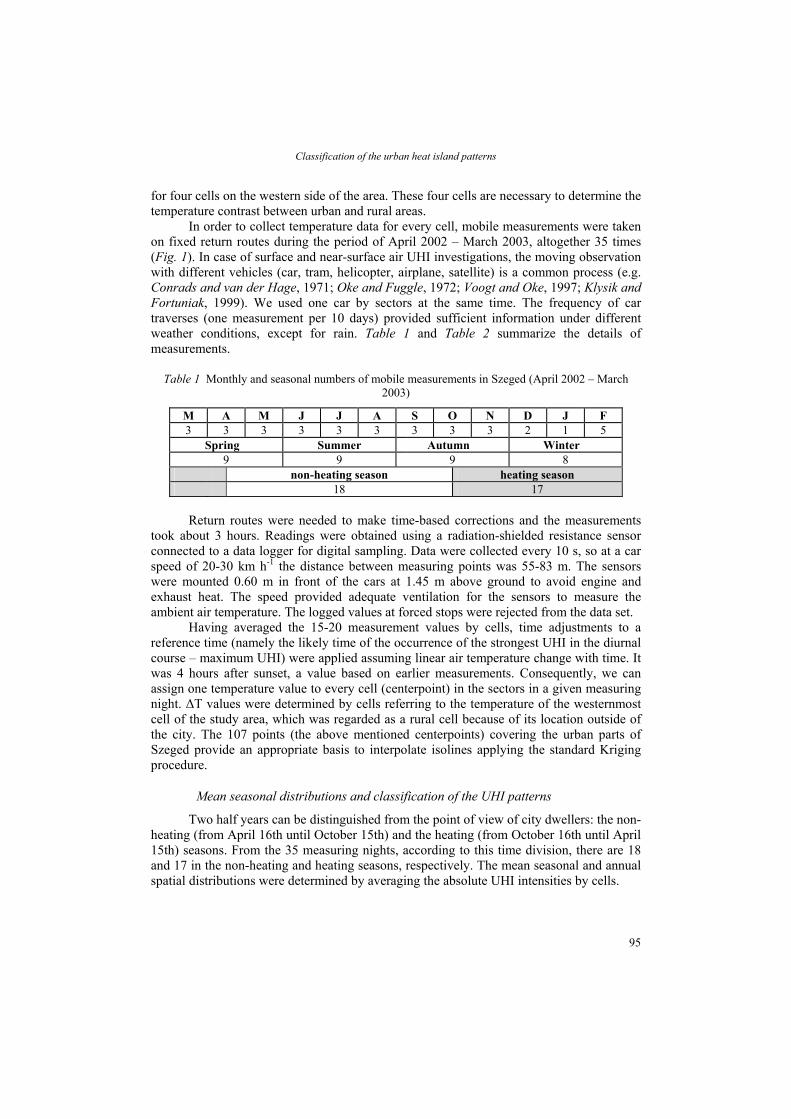
Classification of the urban heat island patterns
for four cells on the western side of the area. These four cells are necessary to determine the temperature contrast between urban and rural areas.
In order to collect temperature data for every cell, mobile measurements were taken on fixed return routes during the period of April 2002 – March 2003, altogether 35 times (Fig. 1). In case of surface and near-surface air UHI investigations, the moving observation with different vehicles (car, tram, helicopter, airplane, satellite) is a common process (e.g. Conrads and van der Hage, 1971; Oke and Fuggle, 1972; Voogt and Oke, 1997; Klysik and Fortuniak, 1999). We used one car by sectors at the same time. The frequency of car traverses (one measurement per 10 days) provided sufficient information under different weather conditions, except for rain. Table 1 and Table 2 summarize the details of measurements.
Table 1 Monthly and seasonal numbers of mobile measurements in Szeged (April 2002 – March 2003)
M A M J J A S O N D J F 3 3 3 3 3 3 3 3 3 2 1 5
Spring Summer Autumn Winter 9 9 9 8 non-heating season heating season 18 17 Return routes were needed to make time-based corrections and the measurements
took about 3 hours. Readings were obtained using a radiation-shielded resistance sensor connected to a data logger for digital sampling. Data were collected every 10 s, so at a car speed of 20-30 km h-1 the distance between measuring points was 55-83 m. The sensors were mounted 0.60 m in front of the cars at 1.45 m above ground to avoid engine and exhaust heat. The speed provided adequate ventilation for the sensors to measure the ambient air temperature. The logged values at forced stops were rejected from the data set.
Having averaged the 15-20 measurement values by cells, time adjustments to a reference time (namely the likely time of the occurrence of the strongest UHI in the diurnal course – maximum UHI) were applied assuming linear air temperature change with time. It was 4 hours after sunset, a value based on earlier measurements. Consequently, we can assign one temperature value to every cell (centerpoint) in the sectors in a given measuring night. ∆T values were determined by cells referring to the temperature of the westernmost cell of the study area, which was regarded as a rural cell because of its location outside of the city. The 107 points (the above mentioned centerpoints) covering the urban parts of Szeged provide an appropriate basis to interpolate isolines applying the standard Kriging procedure.
Mean seasonal distributions and classification of the UHI patterns
Two half years can be distinguished from the point of view of city dwellers: the non-heating (from April 16th until October 15th) and the heating (from October 16th until April 15th) seasons. From the 35 measuring nights, according to this time division, there are 18 and 17 in the non-heating and heating seasons, respectively. The mean seasonal and annual spatial distributions were determined by averaging the absolute UHI intensities by cells.
95

Zoltán Sümeghy and János Unger
Table 2 Survey of mobile measurements in the study area of Szeged in the period of April 1999 – March 2003 (CET – Central European Time)
Measuring period No. Date Northern
sector Southern
sector
Reference time (CET)
max. ∆T (ºC)
1 05. 04. 2002 2h 54m 3h 00m 22.15 0.818 2 15. 04. 2002 2h 51m 3h 00m 22.15 2.567 3 22. 04. 2002 3h 01m 3h 08m 22.45 3.214 4 06. 05. 2002 2h 53m 2h 58m 23.00 2.187 5 15. 05. 2002 2h 53m 3h 04m 23.15 4.843 6 23. 05. 2002 2h 52m 2h 59m 23.30 1.178 7 04. 06. 2002 2h 58m 3h 07m 23.30 4.069 8 13. 06. 2002 2h 57m 3h 02m 23.45 4.753 9 26. 06. 2002 2h 47m 2h 57m 23.45 4.259 10 05. 07. 2002 2h 48m 2h 50m 23.45 4.794 11 15. 07. 2002 2h 51m 2h 57m 23.30 3.477 12 24. 07. 2002 2h 48m 3h 03m 23.30 1.180 13 06. 08. 2002 2h 54m 2h 56m 23.15 0.972 14 21. 08. 2002 2h 49m 2h 57m 22.45 3.832 15 27. 08. 2002 2h 48m 2h 49m 22.30 2.000 16 02. 09. 2002 2h 49m 3h 00m 22.30 1.004 17 18. 09. 2002 2h 51m 2h 57m 22.00 4.467 18 30. 09. 2002 2h 57m 2h 55m 21.30 1.434 19 07. 10. 2002 2h 57m 3h 08m 21.15 3.111 20 14. 10. 2002 3h 03m 3h 05m 21.00 1.833 21 28. 10. 2002 3h 00m 3h 11m 20.30 1.107 22 12. 11. 2002 3h 00m 3h 12m 20.15 2.615 23 18. 11. 2002 2h 57m 3h 01m 20.00 3.207 24 27. 11. 2002 2h 59m 3h 00m 20.00 2.756 25 12. 12. 2002 3h 00m 3h 05m 20.00 0.346 26 20. 12. 2002 3h 06m 3h 06m 20.00 2.403 27 27. 01. 2003 3h 05m 3h 10m 20.30 1.060 28 02. 02. 2003 2h 58m 3h 16m 20.45 4.423 29 17. 02. 2003 3h 01m 3h 14m 21.15 3.938 30 18. 02. 2003 3h 01m 3h 07m 21.15 5.052 31 24. 02. 2003 2h 59m 3h 02m 21.15 1.600 32 26. 02. 2003 3h 04m 3h 05m 21.30 5.055 33 05. 03. 2003 2h 59m 3h 04m 21.30 2.616 34 24. 03. 2003 2h 55m 3h 03m 22.00 6.815 35 25. 03. 2003 2h 57m 3h 03m 22.00 5.476
The first step for the grouping the UHI patterns by the forms was the normalization
of the ∆T values of each pattern. In course of the normalization the absolute intensities by cells were divided by the absolute value of the cell which had the maximum intensity at the given night. This process eliminates the alterations caused by the differences in the UHI magnitude. Then, cross-correlation was applied for the normalized temperature patterns (107 ∆T values) of the 35 measuring nights. It means altogether 595 relationships between the different patterns. For practical purposes, the coefficients can be gather in a cross-correlation matrix (Montavez et al., 2000). In our case the correlation coefficient is significant at the 99% of confidence level if it is larger than 0.25 (n = 107).
96

Classification of the urban heat island patterns
The classification is based on the next simple common feature: those patterns are in a class (or type) which are in the above mentioned significant correlation with each other pattern in the class.
RESULTS AND DISCUSSION
0.5 1.0
Fig. 2 Spatial distribution of the mean max. UHI intensity (ºC) during the investigated one-year period
in Szeged
In both seasons and in the one-year period the shapes of the UHI patterns are almost concentric and the temperature values are increasing from the outskirts towards the inner areas. A large deviation from this shape occurs in the north-eastern part of the city, where the isotherms stretch towards the suburbs. This can be explained by the effect of a large housing estate with high concrete buildings and with high built-up ratio (Bottyán and Unger, 2003). In the whole investigated period the greatest mean intensity (2.72ºC) is found in the central cell. The area of considerable differences (∆T of higher than 2ºC) covers about 30% of the total area (Fig. 2).
0.5 1.0
0.5
1.0 1.5
Fig. 3 Spatial distribution of the mean max. UHI intensity (ºC) during (a) the non-heating season and
(b) the heating season in Szeged
In the half-year seasons the structure of the UHI is very similar to the one-year period, only the highest values differ slightly. In the non-heating season the ∆T is a bit larger (2.79ºC), while in the heating season it is a bit smaller (2.63ºC), than in the one-year period (Fig. 3).
According to the classification of the individual UHI patterns using correlation values, eight types of the form (marked by A, B, ...) can be distinguished. Table 3 contains
97

Zoltán Sümeghy and János Unger
the members (marked by the numbers of measurements, see Table 2) and the ranges of the measured maximum intensities by types. In comparison with the regular, centralized pattern (A), the irregularities (or rather shifts) in the forms are reflected in the names of the types. These shifts
exconoex
A
T
98
Table 3 Names, members and ranges of the measured maximum intensities (ºC) of UHI pattern types
ype Name Members ∆T range A centralized 5, 9, 12, 15, 23, 33 0.35 – 5.48 B shifted to NW 13, 18, 20, 21, 22, 31 1.83 – 3.21 C shifted to N-NE 4, 6, 11, 24, 25 0.97 – 4.75 D shifted to E-SE 1, 27, 28, 35 2.57 – 5.05 E shifted to E-NE 3, 10, 17, 19 1.11 – 4.84 F shifted to W-SW 2, 7, 29 1.60 – 4.26 G shifted to S 14, 16, 34 0.82 – 1.43
can be, presumably, plained by the prevailing wind directions at the given measuring nights, but the exact nfirmation of this relationship needs further data collection and examination. Example rmalized patterns of each distinguished types (except of the miscellaneous type H) are hibited in Fig. 4
.
0.2 0.4
B
Fig. 4 Example patterns by types and their dates in Szeged. The cells with the highest value are
marked by points. A (centralized) – 18. 09. 2002, B (shifted to NW) – 27. 08. 2002
C
D
Fig. 4 (continued) C (shifted to N-NE) – 13. 06. 2002, D (shifted to E-SE) – 18. 02. 2003
H miscellaneous 8, 26, 30, 32 4.42 – 6.81

Classification of the urban heat island patterns
E
0.4 0.6
0.2
F
Fig. 4 (continued) E (shifted to E-NE) – 24. 07. 2002, F (shifted to W-SW) – 26. 06. 2002
CONCLUSIONS
The following conclusions are reached from the analysis presented:
(i) The spatial patterns of the mean UHI intensity have almost concentric shapes. The anomalies in the regularity are caused by the alterations in the urban surface features.
(ii) The normalization of the intensities gave us a useful tool for the comparison and classification of the
individual UHI patterns. Eight types of the ∆T pattern can be distinguished. The shifts in the forms are, with a large probability, in connection with the prevailing wind directions.
G
Fig. 4 (continued) G (shifted to S) – 05. 04.
2002
Acknowledgements – This research was supported by the grant of the Hungarian Scientific Research Fund (OTKA T/034161). The work of the second author was also supported by the Széchenyi István Scholarship of the Ministry of Education (SZÖ 84/2002). The cross-correlation was calculated by Z. Bottyán.
REFERENCES
Bottyán, Z. and Unger, J., 2003: A multiple linear statistical model for estimating mean maximum urban heat island. Theor. Appl. Climatol. 75, 233-243.
Conrads, L.A. and van der Hage, J.C.H., 1971: A new method of air-temperature measurement in urban climatological studies. Atmos. Environ. 5, 629-635.
Klysik, K. and Fortuniak, K., 1999: Temporal and spatial characteristics of the urban heat island of Lódz, Poland. Atmos. Environ. 33, 3885-3895.
Montavez, J.P., Rodriguez, A. and Jimenez, J.I., 2000: A study of urban heat island of Granada. Int. J. Climatol. 20, 899-911.
Oke, T.R. and Fuggle, R.F., 1972: Comparison of urban/rural counter and net radiation at night. Bound. Lay. Meteorol. 2, 290-308.
99

Zoltán Sümeghy and János Unger
Unger, J., Sümeghy, Z., Gulyás, A., Bottyán, Z. and Mucsi, L., 2001: Land-use and meteorological aspects of the urban heat island. Meteorol. Applications 8, 189-194.
Voogt, J.A. and Oke, T.R., 1997: Complete urban surface temperatures. J. Appl. Meteorol. 36, 1117-1132.
100
ACTA CLIMATOLOGICA ET CHOROLOGICA Universitatis Szegediensis, Tom. 36-37, 2003, 101-109.
SEASONAL CASE STUDIES ON THE URBAN TEMPERATURE CROSS-SECTION
Z. SÜMEGHY and J. UNGER
Department of Climatology and Landscape Ecology, University of Szeged, P.O.Box 653, 6701 Szeged, Hungary E-mail: [email protected]
Összefoglalás – A kutatás a városi hősziget (UHI) éjszakai dinamikájára összpontosít a vizsgált település, Szeged esetében. A munka célja az UHI fel- és leépülésének tanulmányozása egy kiválasztott városi keresztmetszet mentén úgy, hogy minden évszakból bemutat egy-egy jellegzetes esetet, amelynek sajátosságait a meteorológiai és területhasznosítási paraméterek figyelembevételével magyarázza. Az UHI kiformálódása meglehetősen szabályos volt: a legmagasabb értékek a városközpontban, pár órával napnyugta után tűntek föl. Mindazonáltal megfigyelhető néhány asszimetria az izotermákban, mert azok mindig eltolódnak a keresztmetszet keleti széle felé. Ez elsősorban annak tulajdonítható, hogy ez egy sűrűn beépített környék. A nyári éjszaka esetében például a normalizált UHI értékek használata a profilok számos speciális vonását tárta föl. A keleti és a nyugati külvárosokban az UHI nagyságában bekövetkező változásokat a hűvösebb vidéki levegő először ÉNy, majd pedig KÉK felől (a szélirány változásával összhangban) történő beáramlása okozta. Az őszi mérés során észlelt kettős csúcs jelensége csak a szélsebbeségben bekövetkezett átmeneti csökkenéssel magyarázható. Summary – Investigations concentrated on the temporal dynamics of the urban heat island (UHI) during the night in Szeged, Hungary. Task includes the revelation of building and re-building of the UHI along an urban cross-section studying example cases by seasons and the explanation of their features using land-use and meteorological parameters. The UHI formations were rather perfect with the highest values in the city centre and a few hours after sunset. However, some assimetry occurs in the isotherms because they are always shifted a bit to the eastern edge of the transect. It can be attributed to the influence of the highest built-up density of this neighbourhood. For example in the case of the summer night using normalized UHI values some interesting features in the profiles emerge. Presumably, the changes in the magnitudes of UHI in the western and eastern suburbs are caused by the cooler rural air transport (first from NW then from E-NE) according to the changed wind direction. The phenomena of the two peaks was observed in the course of the fall measurment and it can be explained only by the temporary decrease of the wind speed.
Key words: UHI, urban cross-section, summer and winter cases, Szeged, Hungary
INTRODUCTION
The climate modification effect of urbanization is most obvious for the temperature (urban heat island – UHI). Its magnitude is the UHI intensity (namely ∆T, the temperature difference between urban and rural areas). In general this intensity has a diurnal cycle with a strongest development of 3-5 hours after sunset.
The purpose of this study is to reveal the temporal dynamics (building and re-building) of the UHI during the night along an urban cross-section investigating some seasonal example cases and to explain their features using land-use and meteorological parameters.
101

Zoltán Sümeghy and János Unger
STUDY AREA AND METHODS
General
The studied city, Szeged, is located in the south-eastern part of Hungary (46°N, 20°E) at 79 m above sea level on a flat plain. The River Tisza passes through the city, otherwise, there are no large water bodies nearby. The river is relatively narrow and according to our earlier investigation its influence is negligible (Unger et al., 2001). These environmental circumstances make Szeged a favourable place for studying of an almost undisturbed urban climate.
Within the city’s administration district of 281 km2, the number of inhabitants is 160,000. The region is in Köppen's climatic region Cf which means a temperate warm climate with a fairly uniform annual distribution of precipitation.
Grid network and temperature (maximum UHI intensity)
The area of investigation (inner part of the administration district) was divided into 0.5 km x 0.5 km cells (Fig. 1). The original study area consists of 107 cells covering the urban and suburban parts of Szeged. The outlying parts of the city, characterized by village and rural features, are not included in the network except for four cells on the western side of the area. These four cells are necessary to determine the temperature contrast between urban and rural areas. In present study we use only 17 cells, which is a cross-section of the urban area consisting each of the typical land-use types of Szeged (Fig. 1). It is streching from the rural area (cell 1) across zones used for industry and warehousing (cells 4-7), the densely-built centre (cell 9-11) and large housing estates of tall concrete buildings set in wide green spaces (13-15) to the areas occupied by detached houses (17). The distance between the centerpoints of the first (1) and the last (17) cells along the cross-section is about 8 km. Basically, the orientation of the cross-section is from W to E-NE.
In order to collect temperature data for every cell during the night, mobile measurements were taken on fixed return routes on an hourly basis along the cross-section between April 2002 and March 2003, altogether 12 times. In case of surface and near-surface air UHI investigations, the moving observation with different vehicles (car, tram, helicopter, airplane, satellite) is a common process (e.g. Conrads and van der Hage, 1971; Oke and Fuggle, 1972; Voogt and Oke, 1997; Klysik and Fortuniak, 1999). To get some information on the temporal dynamics (building and re-building) of the UHI during the night, the measurements started at sunset and took about 7-10 hours (depending on the season), which means 7-10 transects (Table 1). Return routes were needed to make time-based corrections and one transect took about 50-60 minutes. Readings were obtained using a radiation-shielded resistance sensor connected to a data logger for digital sampling. Data were collected every 10 s, so at a car speed of 20-30 kmh-1 the distance between the measuring points was 55-83 m. The sensor was mounted 0.60 m in front of the car at 1.45 m above ground to avoid engine and exhaust heat. The speed provided adequate ventilation for the sensor to measure the momentary ambient air temperature. The logged values at forced stops were rejected from the data set.
Having averaged the approximately 15-20 measurement values by cells, time adjustments to the reference times (namely integer hours after sunset) were applied assuming linear air temperature change with time. Consequently, we can assign one temperature value to every cell (centerpoint) by transects. ∆T values were determined by
102

Seasonal case studies on the urban temperature cross-section
cells referring to the temperature of the westernmost cell of the cross-section, which was regarded as a rural cell because of its location outside of the city (Fig. 1).
Tisza
641 2 3 5 7 8 9 10 11121314 15 16 17
46 15’ NO
20 10’ EO2 km0 1
Fig. 1 Division of the original study area into 0.5 km x 0.5 km grid cells. Cells of the urban cross-
section are numbered from 1 to 17. The urbanized areas are marked by white.
Table 1 Survey of mobile measurements along the cross-section in Szeged (April 2002 - March 2003)
No. Date Time of the sunset (CET)
Number of transects
Reference times
1 16-17. 04. 2002 18.27 10 19.00 – 04.00 2 22-23. 05. 2002 19.13 8 20.00 – 03.00 3 17-18. 06. 2002 19.33 7 21.00 – 03.00 4 10-11. 07. 2002 19.31 7 21.00 – 03.00 5 29-30. 08. 2002 18.24 9 20.00 – 04.00 6 10-11. 09. 2002 18.01 10 19.00 – 04.00 7 17-18. 10. 2002 16.50 10 18.00 – 03.00 8 14-15. 11. 2002 16.08 10 17.00 – 02.00 9 10-11. 12. 2002 15.53 10 17.00 – 02.00 10 15-16. 01. 2003 16.19 10 17.00 – 02.00 11 12-13. 02. 2003 17.00 10 18.00 – 03.00 12 17-18. 03. 2003 17.47 10 19.00 – 04.00
The profiles of the UHI intensity along the cross-section were investigated by comparison of absolute and normalized values taking land-use and meteorological features into consideration. The normalized value of a given cell in a given hour is the ratio of the absolute values of that cell and the cell where ∆T is the largest at that transect. Since meteorological conditions (first of all wind speed and cloudiness) influence the absolute
103

Zoltán Sümeghy and János Unger
UHI intensities (e.g. Landsberg, 1981; Park, 1986; Yagüe et al., 1991, Unger, 1996), the comparison of spatial variation of ∆T is more effective using normalized values. Namely, the normalized UHI intensity profiles are expected to be almost independent of the prevailing weather conditions; nevertheless, they are expected to be dependent mainly on the surface factors (e.g. land-use features, distance from the city centre, etc.).
Present study examines four cases (nights of 16-17 April 2002, 17-18 June 2002, 10-11 September 2002 and 12-13 February 2003) in detail, when the conditions were favourable for relatively strong development of the UHI. The first case represents a pleasant spring night, the second case a warm summer night, the third case a rather warm autumn night and the fourth case a very cold winter night as seasonal example nights.
Built-up surface ratio
Ratios (to total cell area) of the built-up surface by cells were determined by a vector and raster-based GIS database combined with remote sensing analysis of SPOT XS images. The geometric resolution of the image was 20 m x 20 m. Normalized Difference Vegetation Index (NDVI) was calculated from the pixel values, using visible (V: 0.58-0.68 µm) and near infrared (IR: 0.72-1.1 µm) bands (Gallo and Owen, 1999): NDVI = (IR-V)/(IR+V).
The NDVI values are between -1 to +1 indicating the effect of green space in the given spatial unit. Built-up, water and vegetated surfaces were distinguished using these values. The ratios of these land-use types for each grid element were determined using cross-tabulation.
RESULTS AND DISCUSSION
Built-up characteristics
Table 2 contains areal ratios (%) of the main land-use types by cells along the cross-section. The largest built-up density (more than 90%) can be found around the centre (cells 9-10, see Fig. 1), but the variation from the urban edge to the core is not uniform. The proportion of the water surface is rather negligible except for the cell 11 (River Tisza, see Fig. 1). Towards the eastern parts of the city a second high built-up density occurs (cell 15) where the large housing estates are located and the magnitude of the artificial surfaces remained rather significant in the eastern suburbs.
Case 1: the night of 16-17 April 2002
The previous daytime hours were sunny spring hours with a maximum temperature over 20ºC. The sky was almost clear with the highest global radiation flux density of 840 Wm-2 and with light wind (1.3-4.6 ms-1). After sunset (6:27 PM) the wind speed remained in this range. The wind
1
Table 2 Areal ratios of land-use types by cells along the urban cross-section
in Szeged cell built-
up (%) open (%)
water (%)
1 0 100 0 2 0 100 0 3 18.9 81.1 0 4 70.4 23.5 6.1 5 54.2 45.3 0.5 6 85.6 11.1 3.3 7 71.7 28.3 0 8 77.8 22.2 0 9 91.4 8.6 0 10 90.5 9.1 0.4 11 77.3 11.3 11.4 12 83.6 16.4 0 13 75.7 24.3 0 14 67.9 32.1 0 15 81.2 18.8 0 16 60.9 39.1 0 17 72.2 27.8 0
04

Seasonal case studies on the urban temperature cross-section
direction was N-NW at the whole night. During the night a weak anticyclon centered E from Hungary prevailed in the region with an air pressure over 1013 hPa. The sky remained clear and the temperature dropped under 10ºC.
Fig. 2 exhibits the spatial and temporal development of UHI along the cross-section that spring night from the measurements of 10 transects. The UHI formation is rather perfect with the highest (more than 4ºC) values in the city centre (cells 9-12) at 8-9 hours after sunset. In comparison with further cases, there is a time shifting in the highest ∆T values to the late hours of the night, so accordingly
the maximum ∆T value of 4.07ºC occurs at 9 hours after sunset (in cell 10). In every hour the UHI becomes stronger from the rural areas towards the city core and after that it weakens reaching the suburbs on the other side. However, some assimetry occurs in the isotherms because they are shifted a bit to the eastern edge of the transect. This can be attributed to the influence of the highest built-up density of this part contrary to the western cells (Table 2).
10
time
(h)
cell
56
9
4321
789
87654321 10 11 12 13 14 15 16 17
Fig. 2 Isopleths of the UHI intensity (in ºC) along the cross-section during the night of 16-17 April 2002 in Szeged. The unit on the
vertical axis is the elapsed time after sunset.
Case 2: the night of 17-18 June 2002
The previous day was a warm summer day with a maximum temperature over 28ºC. The sky was almost clear with the highest global radiation flux density of 860 Wm-2 and light wind blew (1.8-3.6 ms-1). After sunset (7:33 PM) the wind weakened and its speed was under 2 ms-1 most of the time except for the early morning hours (about 2.5 ms-1 in the period of one hour before sunrise). The wind direction was NW in the first hours after sunset (1-2 hours), then it shifted to N (3-4 hours) and in the last part of the night the wind blew from E-NE (5-7
hours). During the night an anticyclon centered over Hungary prevailed in the region with an air pressure over 1020 hPa. The sky remained clear and the temperature sank under 17ºC.
time
(h)
cell
56
9
4321
7
87654321 10 11 12 13 14 15 16 17
Fig. 3 Isopleths of the UHI intensity (in ºC) along the cross-section during the night of 17-18 June 2002 in Szeged. The unit on the
vertical axis is the elapsed time after sunset.
Fig. 3 summarize the spatial and temporal development of UHI along the cross-section that summer night from the measurements of 7 transects.
105
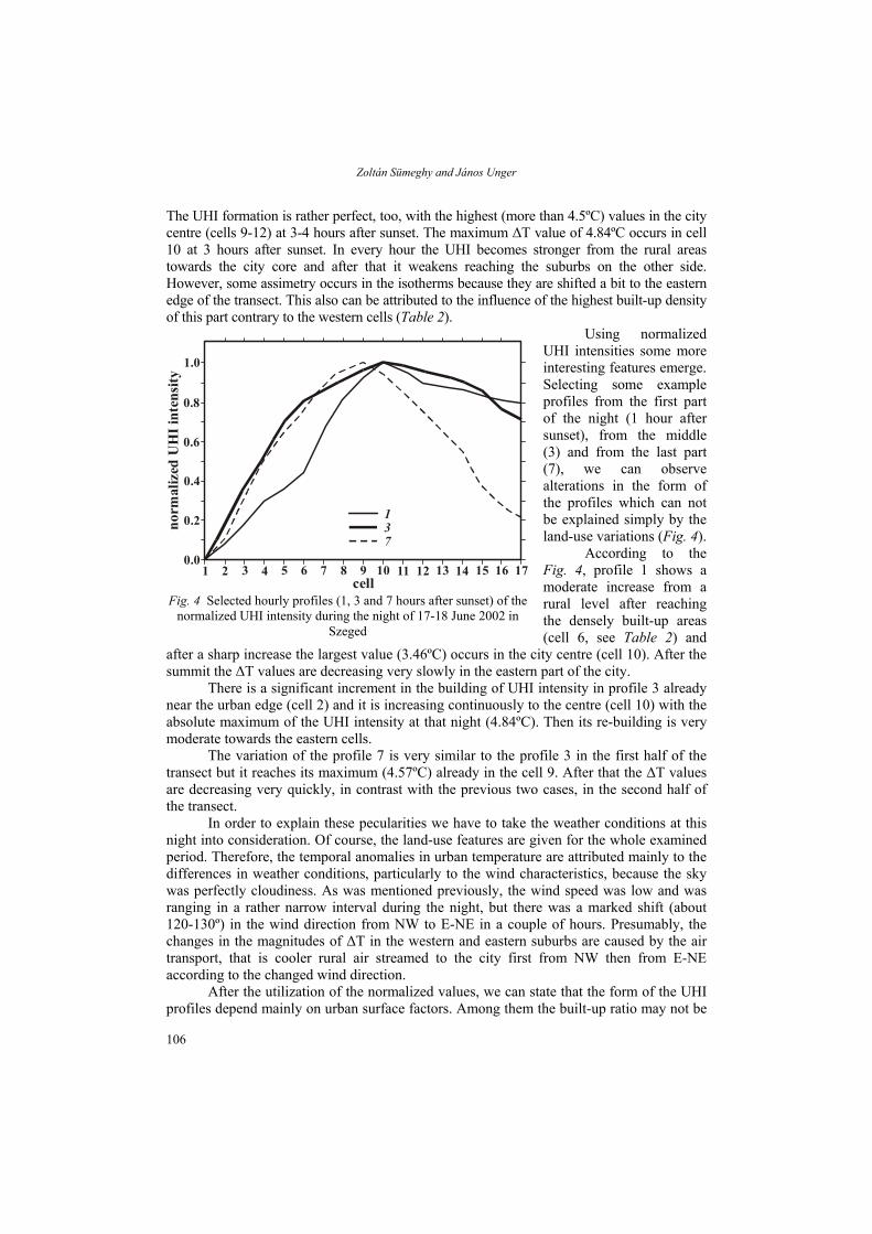
Zoltán Sümeghy and János Unger
The UHI formation is rather perfect, too, with the highest (more than 4.5ºC) values in the city centre (cells 9-12) at 3-4 hours after sunset. The maximum ∆T value of 4.84ºC occurs in cell 10 at 3 hours after sunset. In every hour the UHI becomes stronger from the rural areas towards the city core and after that it weakens reaching the suburbs on the other side. However, some assimetry occurs in the isotherms because they are shifted a bit to the eastern edge of the transect. This also can be attributed to the influence of the highest built-up density of this part contrary to the western cells (Table 2).
Using normalized UHI intensities some more interesting features emerge. Selecting some example profiles from the first part of the night (1 hour after sunset), from the middle (3) and from the last part (7), we can observe alterations in the form of the profiles which can not be explained simply by the land-use variations (Fig. 4).
According to the Fig. 4, profile 1 shows a moderate increase from a rural level after reaching the densely built-up areas (cell 6, see Table 2) and
after a sharp increase the largest value (3.46ºC) occurs in the city centre (cell 10). After the summit the ∆T values are decreasing very slowly in the eastern part of the city.
137
1.0
norm
aliz
ed U
HI i
nten
sity
cell
0.6
9
0.4
0.2
0.0
0.8
87654321 10 11 12 13 14 15 16 17
Fig. 4 Selected hourly profiles (1, 3 and 7 hours after sunset) of the normalized UHI intensity during the night of 17-18 June 2002 in
Szeged
There is a significant increment in the building of UHI intensity in profile 3 already near the urban edge (cell 2) and it is increasing continuously to the centre (cell 10) with the absolute maximum of the UHI intensity at that night (4.84ºC). Then its re-building is very moderate towards the eastern cells.
The variation of the profile 7 is very similar to the profile 3 in the first half of the transect but it reaches its maximum (4.57ºC) already in the cell 9. After that the ∆T values are decreasing very quickly, in contrast with the previous two cases, in the second half of the transect.
In order to explain these pecularities we have to take the weather conditions at this night into consideration. Of course, the land-use features are given for the whole examined period. Therefore, the temporal anomalies in urban temperature are attributed mainly to the differences in weather conditions, particularly to the wind characteristics, because the sky was perfectly cloudiness. As was mentioned previously, the wind speed was low and was ranging in a rather narrow interval during the night, but there was a marked shift (about 120-130º) in the wind direction from NW to E-NE in a couple of hours. Presumably, the changes in the magnitudes of ∆T in the western and eastern suburbs are caused by the air transport, that is cooler rural air streamed to the city first from NW then from E-NE according to the changed wind direction.
After the utilization of the normalized values, we can state that the form of the UHI profiles depend mainly on urban surface factors. Among them the built-up ratio may not be
106
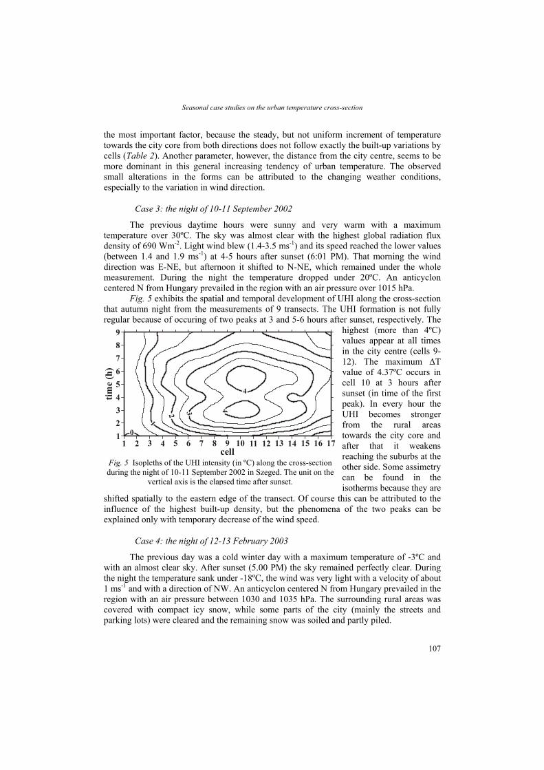
Seasonal case studies on the urban temperature cross-section
the most important factor, because the steady, but not uniform increment of temperature towards the city core from both directions does not follow exactly the built-up variations by cells (Table 2). Another parameter, however, the distance from the city centre, seems to be more dominant in this general increasing tendency of urban temperature. The observed small alterations in the forms can be attributed to the changing weather conditions, especially to the variation in wind direction.
Case 3: the night of 10-11 September 2002
The previous daytime hours were sunny and very warm with a maximum temperature over 30ºC. The sky was almost clear with the highest global radiation flux density of 690 Wm-2. Light wind blew (1.4-3.5 ms-1) and its speed reached the lower values (between 1.4 and 1.9 ms-1) at 4-5 hours after sunset (6:01 PM). That morning the wind direction was E-NE, but afternoon it shifted to N-NE, which remained under the whole measurement. During the night the temperature dropped under 20ºC. An anticyclon centered N from Hungary prevailed in the region with an air pressure over 1015 hPa.
Fig. 5 exhibits the spatial and temporal development of UHI along the cross-section that autumn night from the measurements of 9 transects. The UHI formation is not fully regular because of occuring of two peaks at 3 and 5-6 hours after sunset, respectively. The
highest (more than 4ºC) values appear at all times in the city centre (cells 9-12). The maximum ∆T value of 4.37ºC occurs in cell 10 at 3 hours after sunset (in time of the first peak). In every hour the UHI becomes stronger from the rural areas towards the city core and after that it weakens reaching the suburbs at the other side. Some assimetry can be found in the
sie
wt1rcp
time
(h)
cell
56
9
4321
789
87654321 10 11 12 13 14 15 16 17
Fig. 5 Isopleths of the UHI intensity (in ºC) along the cross-section during the night of 10-11 September 2002 in Szeged. The unit on the
vertical axis is the elapsed time after sunset.
isotherms because they arehifted spatially to the eastern edge of the transect. Of course this can be attributed to the nfluence of the highest built-up density, but the phenomena of the two peaks can be xplained only with temporary decrease of the wind speed.
Case 4: the night of 12-13 February 2003
The previous day was a cold winter day with a maximum temperature of -3ºC and ith an almost clear sky. After sunset (5.00 PM) the sky remained perfectly clear. During
he night the temperature sank under -18ºC, the wind was very light with a velocity of about ms-1 and with a direction of NW. An anticyclon centered N from Hungary prevailed in the egion with an air pressure between 1030 and 1035 hPa. The surrounding rural areas was overed with compact icy snow, while some parts of the city (mainly the streets and arking lots) were cleared and the remaining snow was soiled and partly piled.
107

Zoltán Sümeghy and János Unger
Fig. 6 summarize the spatial and temporal development of UHI along the cross-section that winter night from the measurements of 10 transects. The UHI formation is rather regular with the highest (more than 7.5ºC) values in the broader city centre (cells 10-
14) at 6-8 hours after sunset. The maximum ∆T value of 7.97ºC, which represents a very significant urban modification effect on temperature, occurs in cell 12 at 7 hours after sunset. In every hour the UHI becomes stronger from the rural areas towards the city core and after that it weakens reaching the suburbs at the other side. However, some assimetry can be found in the isotherms because they
are shifted spatially to the eastern edge of the transect more than at the earliaer cases. Moreover, there is a time shifting in the highest ∆T values to the late hours of the night, too, similar to the spring night. Generally, both the areal and temporal extensions of the strong UHI became larger.
10
time
(h)
cell
56
9
4321
789
87654321 10 11 12 13 14 15 16 17
Fig. 6 Isopleths of the UHI intensity (in ºC) along the cross-section during the night of 12-13 February 2003 in Szeged. The unit on the
vertical axis is the elapsed time after sunset.
CONCLUSIONS
The following conclusions are reached from the analysis presented on the seasonal example nights:
(i) The UHI formations were rather perfect with the highest values in the city centre and a few hours after sunset in both cases. However, some assimetry occurs in the isotherms because they are shifted a bit to the eastern edge of the transect. It is obviously the influence of the highest built-up density of this neighbourhood contrary to the western cells.
(ii) Using normalized UHI values some irregularities in the profiles emerge. In autumn the phenomena of the two peaks can be explained only with temporary decrease of the wind speed. In winter the changes in the magnitudes of UHI in the western and eastern suburbs are presumably caused by the cooler rural air transport (first from NW then from E-NE) according to the changed wind direction.
(iii) The usefulness of the normalized values in the investigaton of the cross-section temperature distribution in the urban area is proved. It came to light that the shape of the hourly UHI profile is determined by the surface factors in a high rank but it is sensitive to the momentary weather conditions, especially to the wind direction.
108

Seasonal case studies on the urban temperature cross-section
Acknowledgements – This research was supported by the grant of the Hungarian Scientific Research Fund (OTKA T/034161). The work of the second author was also supported by the Széchenyi István Scholarship of the Ministry of Education (SZÖ 84/2002).
REFERENCES
Conrads, L.A. and van der Hage, J.C.H., 1971: A new method of air-temperature measurement in urban climatological studies. Atmos. Environ. 5, 629-635.
Gallo, K.P. and Owen, T.W., 1999: Satellite-based adjusments for the urban heat island temperature bias. J. Appl. Meteorol. 38, 806-813.
Klysik, K. and Fortuniak, K., 1999: Temporal and spatial characteristics of the urban heat island of Lódz, Poland. Atmos. Environ. 33, 3885-3895.
Landsberg, H.E., 1981: The urban climate. Academic Press, New York. Oke, T.R. and Fuggle, R.F., 1972: Comparison of urban/rural counter and net radiation at night. Bound. Lay.
Meteorol. 2, 290-308. Park, H-S., 1986: Features of the heat island in Seoul and its surrounding cities. Atmos. Environ. 20, 1859-1866. Unger, J., 1996: Heat island intensity with different meteorological conditions in a medium-sized town: Szeged,
Hungary. Theor. Appl. Climatol. 54, 147-151. Unger, J., Sümeghy, Z. and Zoboki, J., 2001: Temperature cross-section features in an urban area. Atmos. Res. 58,
117-127. Voogt, J.A. and Oke, T.R., 1997: Complete urban surface temperatures. J. Appl. Meteorol. 36, 1117-1132. Yagüe, C., Zurita, E. and Martinez, A., 1991: Statistical analysis of the Madrid urban heat island. Atmos. Environ.
25B, 327-332.
109


ACTA CLIMATOLOGICA ET CHOROLOGICA Universitatis Szegediensis, Tom. 36-37, 2003, 111-120.
EFFECTS OF THE SYNOPTIC CONDITIONS ON THE DEVELOPMENT OF THE URBAN HEAT ISLAND IN DEBRECEN, HUNGARY
S. SZEGEDI and A. KIRCSI
Department of Meteorology, University of Debrecen, P.O.Box 13, 4010 Debrecen, Hungary E-mail: [email protected]
Összefoglalás – Cikkünkben a különböző nagytérségi időjárási helyzeteknek a hősziget kialakulására és térbeli szer-kezetére gyakorolt hatását vizsgáljuk Debrecenben. A mobil méréseket gépkocsira szerelt műszerek segítségével hajtottuk végre. Az eredmények igazolták a hősziget meglétét Debrecenben. Kedvező körülmények között (anticik-lonális helyzet, szélcsendes időjárás) a debreceni hősziget speciális jellegzetességeket mutatott. A legszabályosabb szerkezetű hőszigetek olyan esetekben alakultak ki, amikor Magyarország gyenge alacsony- és magasnyomású központok közt helyezkedett el. Anticiklonális helyzetekben erős hőszigetek fejlődtek ki, de az alakjuk rendszerint deformált volt az uralkodó szélirány szerint. Az erős ciklonális helyzetekben a hősziget nem jöhetett létre, míg gyenge ciklontevékenység esetén szabályos, de gyenge, 1ºC körüli intenzitású hőszigetek alakultak csak ki. Summary – In this paper the results of the examinations on the effects of various weather conditions on the development and spatial pattern of the urban heat island (UHI) in Debrecen, Hungary are presented. Measurements were carried out using mobile technique with instruments that were mounted on cars. Examinations proved the existence of the UHI in Debrecen. Under favorable weather conditions (anticyclone activity, calm weather) the heat island showed some unique spatial characteristics. Most regular heat islands developed in cases when Hungary was situated between weak high and low pressure systems. Under antycyclonic conditions strong heat islands formed, but their shape was usually deformed by the prevailing winds. Strong cyclone activity eliminated the formation of the UHI, while under weak cyclone activity regular, but weak heat islands of only about 1ºC developed.
Key words: UHI, mobile measurements, synoptic conditions, spatial distributions
INTRODUCTION
The UHI can develop only under favorable synoptic weather conditions. Anticyclonic conditions presumably are more advantageous for the formation of the heat island because of the undisturbed radiation. Wind can influence the form – or even “blow away” – the heat island. In this study we examine the role of the different synoptic conditions on the formation of the heat island in Debrecen. Under favorable conditions the built up characteristics of the city govern the development of the urban heat island (Magee et al., 1999; Runnals, 1998). The intensity is in close relationship with the size of the city (Oke, 1973; Feng and Petzold, 1988) and its form is determined by the spatial pattern of the built up types.
THE STUDY AREA
Debrecen (21°31’E, 47°38’N) lies at a height of 120 meters above the sea level on the nearly flat terrain of the Great Hungarian Plain (relief is less than 20 meters/1 km),
111

Sándor Szegedi and Andrea Kircsi
which is favorable for studying the development of the urban heat island (Berényi, 1930). It is the second city of Hungary and has a population of 220,000. Debrecen is the cultural and economic center of the north-east region of the country.
In the development of the urban heat island the built up characteristics of the cities play an important role. The important factors are the ratio of the artificial surface cover and the average height and distance of the buildings. On the base of their special characteristics every city’s heat island differs from the general scheme.
Fig. 1 Ratio of the artificial surface cover within the study area in percentage (A: <25% B: 25-50% C:
50-75% D: >75%)
Fig. 2 Location of the study area in Debrecen. A: route of the measurement (north part), B: route of the measurement (south part), C: north part of the grid network, D: south part of the grid network, E:
border of the city.
In Debrecen this specialty lies in that the structure of the city is irregular. Detached and semi detached houses with gardens are dominant in the Eastern sector, where the ratio of the artificial surface cover is between 25 and 50% (Fig. 1).
The ratio of the artificial surface cover is the highest (60-80%) and the average distance of the buildings is the shortest in the downtown near the geometrical center of the city, but the highest buildings cannot be found there but in the housing estates. The large housing estates of Debrecen with 10-14 storey buildings can be found in the Western sector. The ratio of the artificial surface cover is not very high (40-60%), but there are the most extensive vertical active surfaces. Since the houses are built in N-S rows and the distance of the buildings in that direction is minimal (only a few meters) they form quasi-homogenous active surfaces oriented to the East and West. The imbalance is more visible in the N-S direction than in the E-W direction (Fig. 1). The industrial belt of the city is in the Southern sector, where the ratio of the artificial surface cover is between 60 and 80%. On the other side, in the Northern sector can be found the forest of the “Nagyerdő”, which is the first nature conservation area of Hungary. Its urban part, which
112

Effects of the synoptic conditions in the development of the urban heat island in Debrecen, Hungary
belongs to the study area, is an extensive urban park forest (1.75 km2) with sports-grounds, the stadium, the amusement park, the zoo, the clinics and the campus of the University of the city.
Another specialty is that in most places there are not clear borders between the city and its environment: the density of the buildings decreases very gradually because spots of detached houses with gardens alternate with extensive green areas (the ex Soviet airbase, sporting grounds and the forest of the ”Nagyerdő”) along the borders of the city.
METHODS
Measurements were carried out in ten days intervals under various synoptic weather conditions (except the rain, which eliminated the development of the UHI) in order to get information about the impact of the synoptic conditions on the development of the heat island (Unger et al., 2000). The campaign began in the April of 2002 and finished in the March of 2003.
The area of the city was divided into grids of 500 by 500 meters and two routes were established in the Northern and Southern part of the city (Fig. 2). An important problem is that measurements should be carried out in the same point of time in each grid. This is impossible using mobile techniques. The difference between the first and the last grid is 90 minutes, which is a considerable time span from the aspect of the change of the temperature in the different parts of the city. For this reason in order to get comparable temperature data during the measurements we visited each grid two times: first on the way to the end of the rout and the second time on the way back. This way we gained two temperature values for each grid. Since on the way back we visited the grids in just the reverse order calculating the averages for the grids we gained values for the same time (the reference time). The reference time was four hours after sunset since according to the literature (Landsberg, 1981a, 1981b; Unger et al., 2001) the heat island intensity reaches its maximum 3-5 hours after sunset.
Digital thermometers were mounted on cars at a height of 170 cm. The thermometers had a thermal shield to eliminate the radiant heat from the cars engine. Data were recorded on a Logit data logger, the sampling interval was 10 seconds. Datasets were processed using Excel for Windows, maps were made using Surfer for Windows softwares using the kriging interpolation technique.
RESULTS
Spatial pattern of the UHI of Debrecen
Measurements have proved the existence of the heat island in Debrecen. The mean maximal urban heat island intensity was 2.3ºC. The absolute maximal intensity in the studied period was 5.8ºC, which falls behind the values calculated using the Oke’s formula (6.6-6.7ºC) based on the population of the city (Oke, 1973).
The city core and the housing estates in the western sector of the city belong to the center of the heat island (Fig. 3). According to Oke’s terminology (Oke, 1987) the geometrical center of the city should appear as the “peak”, but here the peak is missing and the city center and its neighborhood takes the shape of a broad and very flat ”plateau”. The
113

Sándor Szegedi and Andrea Kircsi
special built-up characteristics of Debrecen can explain this phenomenon: the buildings and consequently the ratio of the vertical active surfaces is not much higher in the city center than in its environment. The ratio of the artificial surfaces is high (70-80%) in the city center, but there are 4-5 storey buildings. A belt of housing estates borders the center of Debrecen from the west, where the ratio of artificial surface cover is still relatively high (over 50%), and there are large vertical active surfaces of the 10-14 storey buildings (Fig. 1).
Fig. 3 Annual mean maximum UHI intensities in Debrecen (°C)
Intensities increase gradually in the Eastern sector of the city towards the center because the built up density grows gradually as well. The forest of the ”Nagyerdő” in the North is the coolest part of the city. The highest horizontal gradients (0.5°C/300 meters) were found there. This is in harmony with the spatial pattern of the natural and artificial surfaces. The ratio of the artificial surface cover is under 30% in the urban part of the forest of the ”Nagyerdő”. It is bordered by low intensity residential areas, the campus of the University of Debrecen and the clinics of the city. It is connected to the trunk of the forest outside the city in the North and for this reason it behaves like a cold fringe of that: it is cooler than its urban environment by 0.5-0.8ºC on annual average.
Seasonal variability – the effect of the synoptic conditions
In the non-heating season the mean maximal UHI intensity reached 2.5ºC, which is higher than that of the whole period (Fig. 4).
It proves that in Debrecen in the non-heating season stronger heat islands develop than in the heating season. The reason for this is that the high pressure system over the subtropical waters of the Atlantic governs the weather of Hungary in the summer except June. The radiation conditions are favorable for the formation of the UHI. The high pressure center cause a Northern air flow in the Carpathian Basin, which is altered by the relief to NE direction in the region of Debrecen (Justyák and Tar, 1984). The wind speeds usually are between 2-5 ms-1.
114

Effects of the synoptic conditions in the development of the urban heat island in Debrecen, Hungary
The absolute maximum was 5.8ºC what was the highest value within the whole studied period. Under anticyclonic conditions strong heat islands developed but the shape often were deformed by the prevailing NE winds. Under such conditions the center of the heat island was drifted southwestward. This situation can clearly be seen in Fig. 5. The heat island in that case developed under strong anticyclone activity: skies had been clear for more than a week with strong irradiance and NE winds blew with a speed of 3 ms-1 during the measurements. Under cyclonic conditions, when the sky was cloudy the intensities hardly exceeded 1ºC.
Fig. 4 Mean maximum UHI intensities in Debrecen (°C) in the non-heating season
Fig. 5 The UHI intensitiy in Debrecen on 26 June 2002 (°C)
115
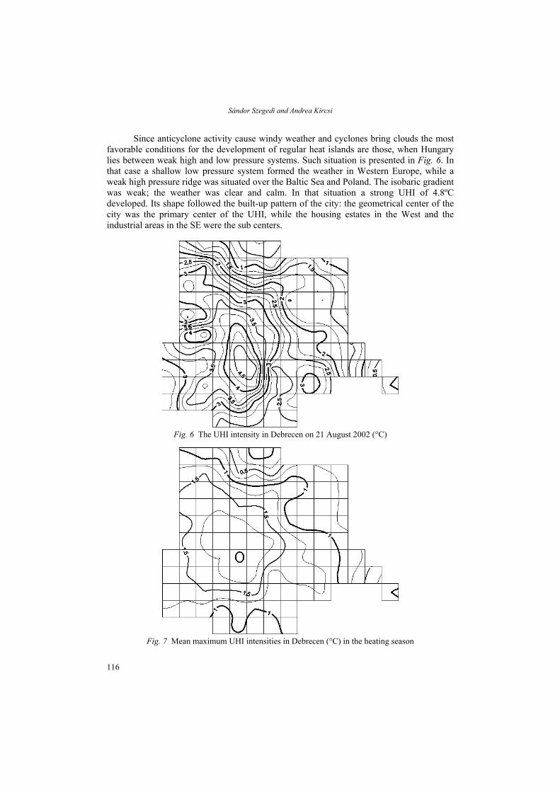
Sándor Szegedi and Andrea Kircsi
Since anticyclone activity cause windy weather and cyclones bring clouds the most favorable conditions for the development of regular heat islands are those, when Hungary lies between weak high and low pressure systems. Such situation is presented in Fig. 6. In that case a shallow low pressure system formed the weather in Western Europe, while a weak high pressure ridge was situated over the Baltic Sea and Poland. The isobaric gradient was weak; the weather was clear and calm. In that situation a strong UHI of 4.8ºC developed. Its shape followed the built-up pattern of the city: the geometrical center of the city was the primary center of the UHI, while the housing estates in the West and the industrial areas in the SE were the sub centers.
Fig. 6 The UHI intensity in Debrecen on 21 August 2002 (°C)
Fig. 7 Mean maximum UHI intensities in Debrecen (°C) in the heating season
116

Effects of the synoptic conditions in the development of the urban heat island in Debrecen, Hungary
In the heating season the mean maximal UHI intensity was 2.1ºC, which is lower than the annual mean and the non-heating season mean value (Fig. 7). The reason for this is that in the winter period (especially in November and December) the cyclonic activity is strong in the Carpathian basin due to the influence of the low pressure system of Iceland.
Fig. 8 The UHI intensity in Debrecen on 18 November 2002 (°C)
Strong heat islands developed under anticyclonic weather conditions with clear skies
and weak NE winds (Fig. 8). The absolute maximum in the central and in the South and SW grids reached 5.5ºC which is not significantly lower than that in the heating season. In the Northern part intensities were usually under 4ºC. From the aspect of the absolute maxima there is not a deep gap between the heating and non-heating season.
Fig. 9 The UHI intensity in Debrecen on 5 March 2003 (°C)
117

Sándor Szegedi and Andrea Kircsi
When snow covered the ground and only walls played the role of the active surfaces the spatial pattern was more uniform. Cloudy weather conditions prevented the development of the heat island, only anthropogenic heat input generated weak heat islands of 1ºC (Fig. 9).
During frontal activity Western winds prevailed therefore the center of the UHI was pushed to the East. This situation is presented in Fig. 10.
Fig. 10 The UHI intensity in Debrecen on 15 April 2002 (°C)
Fig. 11 The UHI intensity in Debrecen on 6 May 2002 (°C)
118

Effects of the synoptic conditions in the development of the urban heat island in Debrecen, Hungary
In the spring under anticyclone activity clear skies combined with high wind velocities. Usually weak, asymmetric heat islands developed under such conditions (Fig. 11).
The autumn is not very windy in Debrecen, the wind velocity reaches its annual minimum, which is favorable for the development of strong heat islands. The weather was cloudy in 2002 therefore regular, but weak heat islands were formed usually in the autumn (Fig. 12).
Fig. 12 The UHI intensity in Debrecen on 14 October 2002 (°C)
CONCLUSIONS
The mean maximum urban heat island intensity was 2.3ºC, while the absolute maximum heat island intensity was 5.8ºC in the studied period in Debrecen. In the non-heating season stronger heat islands were detected than in the heating season, although there was not a significant difference between the absolute maxima of the two periods. The spatial pattern is primarily determined by the built-up characteristics of the city. The intensities are not much higher in the city center than in the housing estates and the industrial areas, which are sub centers of the heat island. The cool pole of the city is the forest of the ”Nagyerdő”, which is cooler than its urban environment by 0.5-0.8ºC on the annual average. In the non-heating and the heating season as well strong heat islands developed under anticyclonic conditions, but their shape was usually deformed by the prevailing NE or W winds. Frontal activity connected to mid latitude cyclones usually prevented the formation of the heat island in both periods. The most regular heat islands developed in situations, when Hungary was situated between weak high and low pressure systems and the for this reason the isobaric gradient force was weak.
119

Sándor Szegedi and Andrea Kircsi
Acknowledgements – The authors thank the National Scientific Research Foundation (OTKA) for its support. The research was supported by the program T/034161. The work of the first author was also supported by the Bólyai János Scholarship of the Ministry of Education (BO/00047/02).
REFERENCES
Berényi, D., 1930: The effect of the building blocks on the nocturnal cooling (in Hungarian). Időjárás 34, 46-49. Feng, J.Z. and Petzold, D.E., 1988: Temperature trends through urbanization in Metropolitan Washington, D.C.,
1945-1979, Meteorol. Atmos. Phys. 38, 195-201. Justyák, J. and Tar, K., 1994: The climate of Debrecen (in Hungarian). KLTE Debrecen, 114-130. Landsberg, H.E., 1981a: City climate. In World Survey of Climatology, General Climatology 3. Amsterdam-New
York-Oxford, 299-344. Landsberg, H.E., 1981b: The urban climate. Academic Press, New York-London-Toronto-Sydney-San Francisco,
83-126. Magee, N., Curtis, J. and Wendler, G., 1999: The urban heat island effect at Fairbanks, Alaska. Theor. Appl.
Climatol. 64, 39-47. Oke, T.R., 1973: City size and the urban heat island. Atmos. Environ. 7, 769-779. Oke, T.R., 1987: Boundary layer climates. Routledge, London-New York. Runnals, K.E., 1998: The urban heat island of Vancouver, BC. The Second Symposium on Urban Environment,
Albuquerque, New Mexico. Unger, J., Bottyán, Z., Sümeghy, Z. and Gulyás, Á., 2000: Urban heat island development affected by urban
surface factors. Időjárás 104, 253-268. Unger, J., Sümeghy, Z., Gulyás, Á., Bottyán, Z. and Mucsi, L., 2001: Land-use and meteorological aspects of the
urban heat island. Meteorol. Applications 8, 189-194.
120

ACTA CLIMATOLOGICA ET CHOROLOGICA Universitatis Szegediensis, Tom. 36-37, 2003, 121-130.
RAGWEED POLLEN CONCENTRATION IN THE FUNCTION OF METEOROLOGICAL ELEMENTS IN THE SOUTH-EASTERN PART OF
HUNGARY
B. VITÁNYI1, L. MAKRA2, M. JUHÁSZ3, E. BORSOS2, R. BÉCZI2 and M. SZENTPÉTERI4
1Bocskai István Secondary and Technical School, Ondi út 1, 3900 Szerencs, Hungary E-mail: [email protected]
2Department of Climatology and Landscape Ecology, University of Szeged, P.O.Box 653; 6701 Szeged, Hungary
3Department of Botany, University of Szeged, P.O.Box 657; 6701 Szeged, Hungary 4Teachers’Training Institute, Juhász Gyula Teachers’ Training Faculty,
University of Szeged; Szeged, Hungary
Összefoglalás – Magyarország lakosságának kb. 30 %-a valamilyen allergiás betegségben szenved, ezek 65 %-a pollen-érzékeny, s e pollen-érzékenységnek legalább 60 %-a a parlagfű pollenjétől ered. Dél-Magyarországon az allergiás betegek, valamint az allergén eredetű asztmás betegségben szenvedők száma az 1960-as évek adataihoz képest 1990-re megnégyszereződött. A magyar Nagyalföld déli része (Szeged) a parlagfű pollenjével a leginkább veszélyeztetett terület nemcsak a Kárpát-medencében, hanem egész Európát tekintve, sőt világméretekben is. A parlagfű (Ambrosia artemisiifolia = Ambrosia elatior) pollenje az összes növényi pollen közül a legagresszívabb. Klinikai vizsgálatok bebizonyították, hogy ez az allergén pollen a legkiterjedtebb, a legkomolyabb egészségügyi következményekkel járó és a legtartósabb pollinózis fő okozója. A tanulmány célja annak vizsgálata, hogy a meteorológiai elemek hogyan befolyásolják a parlagfű pollen koncentrációját egy közepes méretű dél-alföldi városban - Szegeden. A vizsgálat adatbázisát az 1997-2001 közötti ötéves időszak napi parlagfű pollenszámai, valamint 11 meteorológiai elem napi átlagértékei képezik. Mind a pollinációs időszak kezdetének (június 20. – július 13.), mind befejeződésének (október 11-29.) nagy az évi változékonysága. Évente a pollinációs időszak tartama, a parlagfű pollenek átlagos napi száma, illetve összes mennyisége a pollinációs időszakban, valamint a leginkább terhelt nap pollenszáma szignifikáns emelkedő trendet mutatnak. Summary – About 30 % of the Hungarian population has some type of allergy, 65 % of them have pollen-sensitivity, and at least 60 % of this pollen-sensitivity is caused by ragweed. Number of patients with registered allergic illnesses doubled and number of cases of allergic asthma became four times higher by the late 1990s in Southern Hungary comparing to those in 1960s. The short (or common) ragweed (Ambrosia artemisiifolia = Ambrosia elatior) has the most aggressive pollen of all. Clinical investigations prove that its allergenic pollen is the main reason of the most massive, most serious and most long-lasting pollinosis. The aim of the study is to analyse how ragweed pollen concentration is influenced by meteorological elements in a medium-sized city, Szeged, Southern Hungary. The data basis consists of daily ragweed pollen counts and averages of 11 meteorological parameters for the five-year daily data set, 1997-2001. The southern part of the Great Hungarian Plain (Szeged) is the most polluted region with ragweed pollen, not only in the Carpathian basin itself but in Europe and even worldwide, too. Both starting date (between June 20 and July 13) and finishing date (between October 11-29) of the pollination period vary widely. Duration, average daily count, total count and counts on peak days show definite increasing trends, respectively.
Key words: pollen allergy, ragweed pollen concentration, Makra-test, factor analysis, regression analysis
121

Béla Vitányi, László Makra, Miklós Juhász, Emőke Borsos, Rita Béczi and Mária Szentpéteri
POLLEN ALLERGY
Pollen allergy has become a widespread disease by the end of the 20th century. Nowadays, every 5th or 6th person, as an average, suffers from this immune system disease in Europe. Pollinosis involves unpleasant symptoms and can become asthma. It has been proved that persons fallen ill with pollen allergy can not concentrate on their work, feel unwell and can be on sick leave many times.
About 30 % of the Hungarian population has some type of allergy, 65 % of them have pollen-sensitivity, and at least 60 % of this pollen-sensitivity is caused by ragweed. It is a shocking fact that number of patients with registered allergic illnesses doubled and number of cases of allergic asthma became four times higher in Southern Hungary by the late 1990-ies comparing to those 40 years before.
Main plants having been caused pollen allergy in Europe are grasses (Poaceae), birch (Betula), mugwort (Artemisia) and, in Southern Europe, olive-tree (Oleaceae). From 1980-ies a new plant joined them, which spreads extremely aggressively. It appears in more and more countries, its blooming lasts for a long time (in some cases even for three months) and it produces much pollen. Breathing them, characteristic symptoms of pollinosis (coughing, sneeze, nasal discharge, inflammation of mucous membranes of eyes and nose) appear very fast. This is the short (or common) ragweed (Ambrosia artemisiifolia = Ambrosia elatior). [Ambrosia was once the delicious food eaten by the mythical Greek gods to make them live forever. Though the Latin name of ragweed and the Greek name of the mentioned delicious food are the same; however, they are completely different things. Ambrosia was the only food of newborns of gods. It is mentioned in the literature either as a food or as a drink. Ambrosia was imagined to have been made of some kind of honey. Wound curing effect was also attributed to it. Of course, the Greek gods didn’t eat ragweed.] On the other hand, clinical investigations prove that the very allergenic pollen of ragweed is the main reason of most massive, most serious and most long-lasting pollinosis.
Considering annual totals of pollen counts of various plants measured between 1990 and 1996 in Southern Hungary, ragweed produces about half of the total pollen production (47.3 %). Though this ratio highly depends on meteorological factors year by year (in 1990 this ratio was 35.9 %, while in 1991: 66.9 %), it can be considered the main aero-allergen plant (Juhász, 1995).
The aim of our study is to give a short survey on history of ragweed and of its pollen’s effect to humans, then to analyse connection of ragweed pollen counts with meteorological elements in Szeged city.
ORIGIN AND DISTRIBUTION OF RAGWEED
This unpleasant weed has its probable origin in Southern North America. This is a plant that has evolved in reaction to a dry climate and open environment. Among 42 species of the Ambrosia genus, only seaside ragweed (Ambrosia maritima) is native in Europe, namely in the Mediterraneum. Its earliest colonisation occurred in Dalmatia (Croatia), where it was an endemic plant on sandy seashores in the Ragusa (recent name: Dubrovnik, Croatia) and Budva (Montenegro) area and on the islands, firstly described in 1842. In Western Europe, first temporary colonisation of ragweed was reported to be in Brandenburg (Germany) in 1863. On the other hand, four American species have already become
122

Ragweed pollen concentration in the function of meteorological elements in the south-eastern part of Hungary
inhabited. These are as follows: ragweed with mugwort leaves (= short ragweed) (Ambrosia artemisiifolia = Ambrosia elatior), giant ragweed (Ambrosia trifida), perennial ragweed (Ambrosia psilostachya) and silver ragweed (Ambrosia tenuifolia). However, short ragweed is the most widely spread of all (Járai-Komlódi and Juhász, 1993).
Distribution of ragweed in Europe started after the First World War. Seeds of different ragweed species were transferred to Europe from America by purple clover seed shipments and grain imports. In this way, its distribution began probably from European ports: e.g. from Rijeka towards Croatia and Transdanubia (latter region is the western part of Hungary), from Trieste and Genoa towards Northern Italy and from Marseille towards the Rhône valley.
Recently, there are three main regions infected by ragweed in Europe: the valley of Rhône (France), Northern Italy and, the most infected region, the Carpathian Basin (Juhász, 1998). Ragweed pollen came to Switzerland by the southerly winds from Northern Italy and the Rhône valley. Atmosphere of the easternmost part of Austria is also sufficiently polluted. It is supposed that ragweed pollen is imported from Hungary to air of Burgenland and Vienna during August and September, when south-east winds are predominant in the region. Jäger and Litschauer (1998) detected pollen of ragweed originated from Transdanubia in the air of Vienna.
The source region of ragweed in Slovakia is Csallóköz (i.e. the plain of Danube) and Eastern Slovakia. The first description of its presence (Komárno, Southwest Slovakia) dated back to 1949. Seeds are partly native, partly they come by the southerly winds from Hungary. Also, they were probably introduced with cereals from the former Soviet Union (Makovcová et al., 1998).
Highest values of ragweed pollen concentrations in Czech Republic occur when south-east winds prevail. This suggests that pollen is not of local origin but come mainly from South-western Slovakia and even from Hungary (Rybnícek, 1998).
Short ragweed arrived at Slovenia at the end of the Second World War. The firstly published map of its distribution dates back to 1978. Its appearance was considered to be temporary. However, ragweed spread widely very fast. Its main regions are lowlands of the country, where ragweed grows as a weed on fields (Seliger, 1998).
In Russia, ragweed invasion is also a big problem. Most contaminated areas are Krasnodar, Stavropol and Sochi in the southern European part of the country (Juhász, 1998).
RAGWEED IN HUNGARY
In Hungary, its appearance was noticed at the beginning of the 20th century at Orsova, near the southern border of the country, along the bank of the Danube. One of the popular names of ragweed in Hungary is „Serbian grass”, which also refers to its place of origin. Ragweed with mugwort leaves (short ragweed) got acclimatised most rapidly; only this species lives here widely. Samples of short ragweed were found in the southern part of Transdanubia in the 1920-ies, and gradually – within 30 years – they occupied the whole region. Since then, having been spread all over the country, it has become the most common weed in Hungary. However, when airborne pollen composition in Szeged (southern part of the Great Hungarian Plain) was analysed in 1968, no any ragweed pollen were found there (Simoncsics et al., 1968). In the southern part of the Great Hungarian Plain there have been more favourable habitats, therefore all stages of the life-cycle (germination, growth,
123

Béla Vitányi, László Makra, Miklós Juhász, Emőke Borsos, Rita Béczi and Mária Szentpéteri
flowering, seed production) start earlier and last longer than those in other parts of the country.
CLIMATOLOGICAL BACKGROUND
There are many reasons of its rapid spread. Hungary belongs to the climate region of Köppen’s Cf (warm-temperate climate with uniform annual distribution of precipitation) or Trewartha D1 (continental climate with longer warm period). Consequently, the climate here is favourable for growing, long-lasting blooming and reaching considerable seed production of ragweed. Its seeds are produced from a few thousands, up to 60,000 seeds by every plant and every year and have a long survival period in the ground (from 5 years up to more than 20 years).
ECOLOGICAL BACKGROUND
The flowering peak of ragweed in Hungary is in August but it may flower from the second half of July to the end of October. Flowers bloom only if the pollen has already ripened. Timing and manner of pollination depend greatly on meteorological factors, first of all on temperature, humidity and light. Increasing temperature and decreasing humidity enhance pollination. It has been observed that pollination starts around 8 a.m., when temperature is increasing and humidity is decreasing as a result of the sunlight and ends around noon. Daily pollen production of ragweed is unimodal with a maximum around noon.
AGRICULTURAL BACKGROUND
Ragweed is not only one of the most dangerous aero-allergen plants but is very noxious weed in agriculture, too. Being a ruderal plant, ragweed is as frequent on roadsides, railway embankments, waste places as in cultivated lands. It can overgrow alfalfa and purple clover entirely, causes severe damages in potato fields and occurs often in sunflower and corn fields, as well. It appears in large quantities among stubbles in the Great Hungarian Plain. Since ragweed is not an old adventive species of the Hungarian flora, it has not got any natural competitors. Light stimulates its germination; hence, waste lands and mixed soils are very soon infested by ragweed. Conditions of soils in Hungary are ideal for its colonisation and growing. Therefore, it has widespread and homogenous cultures all over Hungary. Owing to its special abilities, it can displace other plants, even perennials, and in the lack of competition it becomes dominant. Furthermore, ragweed has less sensitivity to herbicides than other weeds. Because of its here-mentioned characteristics and favourable conditions, ragweed is one of the most studied of non-economic plants.
SOCIAL BACKGROUND
Besides, recent social changes also supported rapid distribution of ragweed. After changing of the political system in 1989, agricultural fields, which had belonged to co-
124

Ragweed pollen concentration in the function of meteorological elements in the south-eastern part of Hungary
operatives, were cut into smaller parcels due to privatisation all over the country. The basic requirement remained to cultivate the land and keep it free from weeds but once being within the property, the new owners did not mind regulations. Realising the danger, a countrywide anti-ragweed campaign was launched in the frame of the National Environmental Health Action Programme. Hundreds of the 3,600 Hungarian settlements introduced special regulations against ragweed pollution. The campaign was supported by the Ministry of Welfare.
ERISTICS OF SZEGED
Szeged (20º06'E; 46º15'N) lies near the confluence of the Tisza and Maros Rivers. It is the largest city in the south-eastern part of Hungary (Fig. 1). The number of inhabitants of the city is up to 160,000 and the surface of its built-up area is about 46 km2. Though Szeged and its surroundings is flat and open region, the city has the lowest elevation in Hungary.
The basis of the city structure is a boulvard-avenue street system crossed by the River Tisza (Fig. 1). In this way the structure of the city is simple however, following to this system, motor vehicle traffic as well as air pollution are concentrated in the city. The industrial area is located mainly in the north-west part of the town. Thus the prevailing westerly and northerly winds transport the pollutants originating from this area towards the centre of the city.
F
voonUnloc(EEn
medame
CLIMATIC CHARACT
Tisza
1
0 5 km
ig. 1 Geographical position of Szeged, Hungary
and built-in types of the city [a: city centre (2-4-storey buildings); b: housing estates with
prefabricated concrete slabs (5-10-storey buildings); c: detached houses (1-2-storey
buildings); d: industrial areas; e: green areas; (1): monitoring station]
DATA
In Szeged, pollen content of the air has been examined with the help of a high lume pollen trap (Lanzoni VPPS 2000) since 1989. The air sampler is found in the city, the roof (20 m height from the city surface) of the building of Faculty of Arts, iversity of Szeged. Meteorological data were obtained from the monitoring station ated 2 km from the sampling site in the downtown, which is operated by the ATIKÖFE
nvironmental Protection Inspectorate of Lower-Tisza Region, Branch of the Ministry of vironment).
The data basis consists of diurnal ragweed pollen counts and averages of 13 teorological parameters for not only the main pollination periods (MPP), but the whole
ta basis of the years 1997-2001, as well. The meteorological parameters are as follows: an air temperature [Tmean (°C)], maximum air temperature [Tmax (°C)], minimum air
125

Béla Vitányi, László Makra, Miklós Juhász, Emőke Borsos, Rita Béczi and Mária Szentpéteri
temperature [Tmin (°C)], diurnal temperature range [∆T (°C)], relative humidity [RH (%)], irradiance [I (Wm-2)], wind speed [WS (ms-1)], vapour pressure [VP (mb)], saturation vapour pressure [E (mb)], potential evaporation [PE (mm)] dew point temperature [Td (°C)], diurnal sum of precipitation [P (mm)] and intensity of precipitation [PI (mm/min)]. The criterion of MPP was introduced by Nilsson and Persson (1981), which takes into account 90 % of the annual total pollen concentration, eliminating the initial 5 % and the final 5 %.
The ragweed pollen count and the mean air temperature of the previous day as well as those of the preceding 2nd and 3rd days are also taken into consideration. Furthermore, average diurnal pollen counts for the analysed period 1997-2001 are also used.
RAGWEED POLLEN COUNTS IN EUROPE, HUNGARY AND SZEGED
Table 1 shows the list of some highest counts on peak days (as a comparison, data of some sites in Pennsylvania, USA are also presented), while Table 2 displays annual totals of ragweed pollen grains.
All the highest counts are reported from the Carpathian Basin, Serbia and Hungary. Novi Sad (Serbia), the southern part of the Great Hungarian Plain (Szeged) and Southwest Hungary (Pécs) are the regions most polluted with ragweed pollen not only in the Carpathian Basin itself but in Europe, too. No higher count than 3247 pollen grains per m3 of air (Novi Sad) has been measured in Europe. The highest values observed in Novi Sad and Szeged on peak days are about one order of
of EupeakvalueEurototalas th
T
Nov
SzeSzeSzePécBudNov
PozPozLju
July,The incre
five-high
126
able 1 Ragweed pollen count on peak days (list of some highest reported counts),
pollen grains / m3 air City Country Year Counts on
peak days i Sad Serbia-
Montenegro 2001 3,247
ged Hungary 1991 2,003 ged Hungary 1994 1,899 ged Hungary 1992 1,658 s Hungary 1994 1,394 apest Hungary 1996 1,254 i Sad Serbia-
Montenegro 1999 723
sony Slovakia 1995 391 sony Slovakia 1997 267 bljana Slovenia 1997 118
magnitude higher than those in other cities rope and the United States, which are considered to be rather polluted. On the reported
days, there is more ragweed pollen even in the air of Budapest, having the lowest among the listed Hungarian cities, than the total amount for the cities listed from pe and the United States having highest values (Table 1). When considering annual s, the highest ragweed pollen counts in Novi Sad and Szeged are many times as much e total amount for the most polluted cities listed from the rest of Europe (Table 2).
The starting date of the pollination period varies widely, between 20 June and 13 whereas the finishing date (between 11-29 October) show a much more limited range. duration, average diurnal count and total count, except for 1998, show definite asing trends.
Characteristics of the main pollination period of ragweed pollen for the examined year data set, as well as their averages are shown in Table 3a. These characteristics ly depend on the meteorological background (Makra et al., 2002).
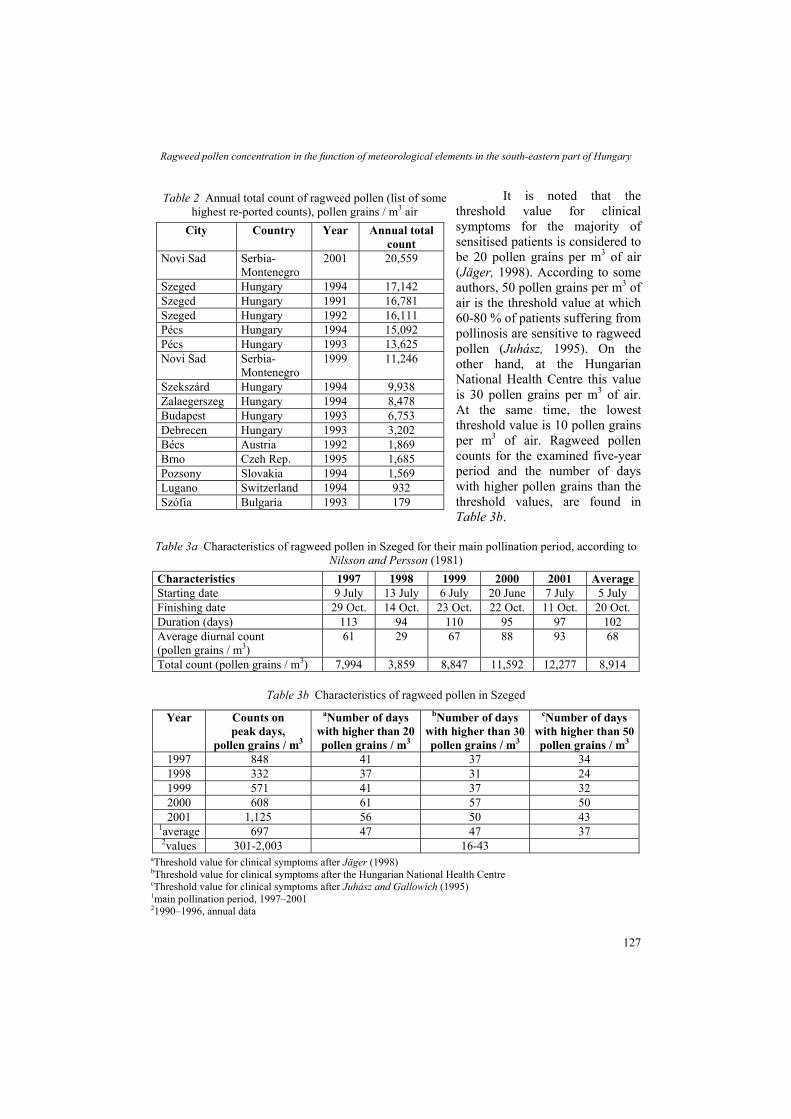
Ragweed pollen concentration in the function of meteorological elements in the south-eastern part of Hungary
It is noted that the threshold value for clinical symptoms for the majority of sensitised patients is considered to be 20 pollen grains per m3 of air (Jäger, 1998). According to some authors, 50 pollen grains per m3 of air is the threshold value at which 60-80 % of patients suffering from pollinosis are sensitive to ragweed pollen (Juhász, 1995). On the other hand, at the Hungarian National Health Centre this value is 30 pollen grains per m3 of air. At the same time, the lowest threshold value is 10 pollen grains per m3 of air. Ragweed pollen counts for the examined five-year period and the number of days with higher pollen grains than the threshold values, are found in Table 3b.
Table 2 Annual total count of ragweed pollen (list of some highest re-ported counts), pollen grains / m3 air
City Country Year Annual total count
Novi Sad Serbia-Montenegro
2001 20,559
Szeged Hungary 1994 17,142 Szeged Hungary 1991 16,781 Szeged Hungary 1992 16,111 Pécs Hungary 1994 15,092 Pécs Hungary 1993 13,625 Novi Sad Serbia-
Montenegro 1999 11,246
Szekszárd Hungary 1994 9,938 Zalaegerszeg Hungary 1994 8,478 Budapest Hungary 1993 6,753 Debrecen Hungary 1993 3,202 Bécs Austria 1992 1,869 Brno Czeh Rep. 1995 1,685 Pozsony Slovakia 1994 1,569 Lugano Switzerland 1994 932 Szófia Bulgaria 1993 179
Table 3a Characteristics of ragweed pollen in Szeged for their main pollination period, according to
Nilsson and Persson (1981) Characteristics 1997 1998 1999 2000 2001 Average Starting date 9 July 13 July 6 July 20 June 7 July 5 July Finishing date 29 Oct. 14 Oct. 23 Oct. 22 Oct. 11 Oct. 20 Oct. Duration (days) 113 94 110 95 97 102 Average diurnal count (pollen grains / m3)
61 29 67 88 93 68
Total count (pollen grains / m3) 7,994 3,859 8,847 11,592 12,277 8,914
Table 3b Characteristics of ragweed pollen in Szeged
Year Counts on peak days,
pollen grains / m3
aNumber of days with higher than 20 pollen grains / m3
bNumber of days with higher than 30 pollen grains / m3
cNumber of days with higher than 50 pollen grains / m3
1997 848 41 37 34 1998 332 37 31 24 1999 571 41 37 32 2000 608 61 57 50 2001 1,125 56 50 43
1average 697 47 47 37 2values 301-2,003 16-43
aThreshold value for clinical symptoms after Jäger (1998) bThreshold value for clinical symptoms after the Hungarian National Health Centre cThreshold value for clinical symptoms after Juhász and Gallowich (1995) 1main pollination period, 1997–2001 21990–1996, annual data
127

Béla Vitányi, László Makra, Miklós Juhász, Emőke Borsos, Rita Béczi and Mária Szentpéteri
During the examined period, both the total counts and counts on peak days increase with fluctuations. Diurnal ragweed pollen counts are over 50 pollen grains per m3 of air for 24-50 days of its 3-months long season, which means severe pollen load of the air. According to the data, the number of days with higher than the threshold values increase, as well.
Comparing results of the two periods (1990–1996, annual data; 15 July – 15 October, 1997–2001), latest values seem to be less extreme. However, the number of days with higher than 30 pollen grains per m3 of air increased definitely in the recent period.
OTHER CHARACTERISTICS OF RAGWEED POLLEN CONCENTRATION
We determined whether or not significant differences can be found between the average of an arbitrary sub-sample of the mentioned time series and that of the whole sample. In our calculations five-year diurnal averages of the daily pollen counts were considered. It was found that averages of the sub-samples with periods between 15 July – 14 August and 17 September – 10 October are significantly lower than that of the whole sample, while the average of the period between 16 August – 13 September is significantly higher than that of the whole sample. This means that, according to the
Ainm
a o
m
vatocoAininbeto
12
-100
-50
0
50
100
150
200
250
300
350
400
15.0
719
.07
23.0
7
27.0
731
.07
04.0
8
08.0
812
.08
16.0
8
20.0
824
.08
28.0
8
01.0
905
.09
09.0
9
13.0
917
.09
21.0
9
25.0
9
29.0
903
.10
07.1
0
11.1
015
.10
Polle
n gr
ains
/ m
3
significantperiod,15.07.-14.08.
significantperiod,16.08.-13.09.
significantperiod,17.09.-15.10.
Ambrosia
Fig. 2 Sub-periods with significantly different verages of ragweed pollen counts from the meanf the entire data series, i.e. the “breaks”, diurnal
average pollen counts, Szeged, 15 July – 15 October, 1997-2001
examined data set, the period between 16ugust – 13 September can be considered to be the most polluted one by ragweed pollen the air; hence, the most dangerous one for pollinosis (Fig. 2). The result received by this ethod confirms data of traditional pollen calculations.
CONNECTION OF RAGWEED POLLEN CONCENTRATION WITH METEOROLOGICAL ELEMENTS
In order to analyze the connection between ragweed pollen concentration and eteorological elements, multivariate statistical analysis was applied (SPSS 9.0 version).
Factor analysis makes it possible to represent connections among the original 12 riables by far less number of so called “theoretical variables” so that these factors gether explain as much information of original variable, as possible. Using this procedure, nnections among many variables can be interpreted and evaluated more easily. ccording to this method, information obtained on the original 12 variables was condensed to 4 theoretical variables; namely, into 4 factors, which together explain 90 % of formation of the original variables. Connections among variables within each factor can explained by the so called factor loadings belonging to the variables (Table 4). In order rank effects of meteorological variables on ragweed pollen concentration (namely, to
8

Ragweed pollen concentration in the function of meteorological elements in the south-eastern part of Hungary
classify variables partly as essential and partly as unimportant ones), special transformation of Factors 1, 2, 3 and 4 to Factor 1 was required. Results are shown in Table 5.
Of all meteorological variables, only wind speed (WS) indicates significant (and positive) connection with ragweed pollen concentration. Though the other variables were also ranked, their effect – according to their factor loadings – cannot be measured. When wind is strengthening, a vast amount of ripe ragweed pollen come to the air and – according to our result – only this meteorological element modifies substantially the concentration of ragweed pollen.
CONCLUSION
Parameters of ragweed pollen [maximum daily concentration per year; total number per year; first observation day; last observation day; duration (day); average daily number; number of days exceeding threshold value of clinical symptoms (20-30-50 pollen grains per m3 per day)], with slight fluctuations, show increasing trends.
Table 4 Factor loadings of the rotated component matrix. Loadings higher than 205.0 are written by bold
Parameters Factor 1 Factor 2 Factor 3 Factor 4 pollen 0.226 -0.005 0.232 0.740 Tmean 0.973 0.184 0.012 0.108 E 0.973 0.183 0.001 0.095 Td 0.961 -0.209 -0.044 0.116 VP 0.960 -0.210 -0.056 0.100 Tmax 0.929 0.222 0.216 0.070 Tmin 0.830 0.053 -0.517 0.090 PE 0.738 0.626 0.072 0.066 RH 0.014 -0.954 -0.140 0.029 I 0.054 0.889 0.058 -0.029 ∆T 0.006 0.193 0.943 -0.035 WS 0.018 -0.036 -0.319 0.749 Eigenvalue 6.145 2.470 1.163 1.018 Explained variance, % 51.209 20.580 9.690 8.486 Cumulative variance, % 51.209 71.789 81.479 89.965
Ragweed pollen load of Szeged is most serious between 16 August – 13 September. Hence, this is the most dangerous period for hay-fever. The above-mentioned period of highest pollen concentration, established by the Makra-test, confirms results of empirical pollen calculations. Application of factor analysis reduced dimension of the original data set (daily ragweed pollen concentration and the examined 11 meteorological variables) in order to detect connections among them more easily. After performing factor analysis, 4 factors were retained according to the Guttmann-criterion. These 4 factors explain 90 % of the total variance of the original 12 variables.
129

Béla Vitányi, László Makra, Miklós Juhász, Emőke Borsos, Rita Béczi and Mária Szentpéteri
Connections among variables, within each factor, can be well interpreted on the basis of their significant factor loadings. After performing special transformation, we concluded that among all the 11 meteorological variables only wind speed (WS) modifies substantially ragweed pollen concentration.
Acknowledgement - The authors thank Gábor Motika (Environmental Protection Inspectorate of Lower-Tisza Region, Szeged, Hungary) for handing monitoring data of the air pollutants and meteorological elements to our disposal; Szilvia Horváth (Department of Climatology and Landscape Ecology, University of Szeged, Hungary) and Predrag Radisic (Laboratory of
SerEco
cofac
Jäg
Jäg
JárJuh
Juh
Juh
Ma
Ma
Nils
Ryb
Seli
Sim
130
Table 5 Effect of variables on daily pollen ncentration and rank of them on the basis of tor loadings specially transformed to Factor 1
Variables Factor 1 Rank pollen 0.740 – Tmean 0.102 3 E 0.089 5 Td 0.109 2 VP 0.093 4 Tmax 0.065 7 Tmin 0.081 6 PE 0.062 8 RH 0.028 11 I -0.029 9-10 ∆T -0.029 9-10 WS 0.747 1
Palinology and Ecology, University of Novi Sad, bia) for valuable contribution and Zoltán Sümeghy (Department of Climatology and Landscape logy, University of Szeged, Hungary) for digital maping.
REFERENCES
er, S., 1998: Global aspects of ragweed in Europe. Satellite Symposium Proc.: Ragweed in Europe. 6th Int’l Congress on Aerobiology, Perugia, Italy, 31.08. – 05.09. 1998. 6-8.
er, S. and Litschauer, R., 1998: Ragweed (Ambrosia) in Austria. Satellite Symposium Proceedings: Ragweed in Europe. 6th International Congress on Aerobiology, Perugia, Italy, 31.08. – 5.09. 1998. 22-26.
ai-Komlódi, M. and Juhász, M., 1993: Ambrosia elatior (L.) in Hungary (1989-1990). Aerobiologia 9, 75-78. ász, M., 1995: New results of aeropalynological research in Southern Hungary. Publications of the Regional
Committee of the Hungarian Academy of Sciences, Szeged 5, 17-30. ász, M. and Gallowich, E., 1995: Comparative aeropalynological study of ragweed pollution of Szeged and Pécs
(Southern Hungary). In: Environmental damages and the respiratory system, 5, p. 244. Eds: Schweiger, O. – Szabó, T. Szentmihályi Press, Zalaegerszeg.
ász, M., 1998: History of ragweed in Europe. Satellite Symposium Proceedings: Ragweed in Europe. 6th International Congress on Aerobiology, Perugia, Italy, 31.08. – 5.09. 1998. 11-14.
kovcová, S., Zlinká, J., Mikolás, V., Salát, D. and Krio, V., 1998: Ragweed in Slovak Republic. Satellite Symposium Proceedings: Ragweed in Europe. 6th International Congress on Aerobiology, Perugia, Italy, 31.08. – 5.09. 1998. 27-28.
kra, L., Horváth, Sz., Pongrácz, R. and Mika, J., 2002: Long term climate deviations: an alternative approach and application on the Palmer drought severity index in Hungary. Physics and Chemistry of the Earth 27, 1063-1071.
son, S. and Persson, S., 1981: Tree pollen spectra in the Stockholm region (Sweden), 1973-1980. Grana 20, 179-182
nícek, O., 1998: Ragweed in the Czeh Republic. Satellite Symposium Proceedings: Ragweed in Europe. 6th International Congress on Aerobiology, Perugia, Italy, 31.08. – 5.09. 1998. 29-32.
ger, A.K., 1998: Ragweed in Slovenia. Satellite Symposium Proceedings: Ragweed in Europe. 6th International Congress on Aerobiology, Perugia, Italy, 31.08. – 5.09. 1998. 39-41.
oncsics, P., Osváth, P. and Balázs, I., 1968: Qualitative analysis of pollen composition in the air. Rheumatologia, Balneologia, Allergologia 9, 117.
NOTES TO CONTRIBUTORS OF ACTA CLIMATOLOGICA ET CHOROLOGICA
Authors may be of any nationality, but the official language of the journal is English. Papers will be reviewed by unidentified referees. Manuscripts should be sent to Editor-in-chief of ACTA CLIMATOLOGICA ET CHOROLOGICA Department of Climatology and Landscape Ecology University of Szeged P.O.Box 653, 6701 Szeged, Hungary in two copies including all illustrations.
Title part of the paper should contain the concise title, the name(s) of the author(s), the affiliation(s) including postal and E-mail address(es). In case of multiple authors, the cover letter should indicate the corresponding author.
Summary should follow the title, it contains the purpose, the data and methods as well as the basic conclusion. A summary in Hungarian as Összefoglalás is expected from Hungarian author(s).
Key words are necessary to help to classify the topic. The text has to be typed in 1.5 spacing with wide margins. Word-processor printing is
preferred. The use of SI units are expected. The negative exponent is preferred to solidus. Figures and tables should be consecutively numbered and referred to in the text.
Mathematical formulas are expected to be as simple as possible and numbered in parentheses at the right margin.
Tables and figures should be marked Arabic numbers (Table 1, Fig. 1) and set in the text together with their captions. Avoid too lengthy or complicated tables.
References: The text citation should contain the name(s) of the author(s) in Italic letter and the year of publication. In case of one author: Johnson (1989), or if the name of the author cannot be fitted into the text: (Johnson, 1989); in the case of two authors: Oke and Maxwell (1975); if there are more than two authors: Smith et al. (1990). When referring to sevaral papers publshed in the same year by the same author, the year of publication should be followed by letters a, b etc. At the end of the paper the list of references should be arranged alphabetically. For an article: the name(s) of author(s) in Italics, year, title of article, name of journal, volume number (the latter two in Italics) and pages. E.g. Jauregui, E., 1989: The dust storms of Mexico City. Int. J. Climatol. 9, 169-180. For a book: the name(s) of author(s), year, title of the book (all in Italics except the year), publisher and place of publication. E.g. Junge, C.E., 1963: Air Chemistry and Radioactivity. Academic Press, New York and London.
The final version should be submitted on CD altogether with one hard copy. The preferred medium for the text is MS Word 2002 (or Office XP) and for the figures the CorelDraw 9 or Excel 2002 (or Office XP) (or in 300 dpi resolution, high quality .JPG or .TIF formats).
Reprints: authors receive 1 copy of the relevant issue and 20 reprints free of charge. More information: [email protected]
[email protected] [email protected]
131


![EümérnökiMSc Lemorzsolódás v2.pptx [Read-Only])home.mit.bme.hu/~jobbagy/eum/elorehaladas.pdfDebreceni Egyetem 2 Szegedi Tudományegyetem 2 Pécsi Tudományegyetem 2 Szent István](https://img.pdfslide.us/doc/110x75/5e60939fdc36ff4f3d4307c1/emrnkimsc-lemorzsolds-v2pptx-read-onlyhomemitbmehujobbagyeum.jpg)