Contents · Poset Isomorphisms and Duality 7 1.8. Antichains and Order Ideals 7 1.9. Operations on Posets 8 2. Graded Posets 8 2.1. Rank Functions 8 2.2. Graded Posets 9 ... The Lattice

COMBINATORIAL ASPECTS OF PARTIALLY ORDERED SETS

BERTON A. EARNSHAW

Dedicated to my wife Tiraje, who I love.

Abstract. This set of notes is prepared for the Meander Group (MG) atBrigham Young University. Its purpose is to introduce MG to:(1) the basic definitions and theorems of partially ordered set theory and(2) the various combinatorial methods associated with partially ordered sets.

Contents

List of Figures 21. Partially Ordered Sets 21.1. Partially Ordered Sets 21.2. Subposets 31.3. Locally Finite Posets 41.4. Hasse Diagrams 41.5. Minimal and Maximal Elements 51.6. Chains 61.7. Poset Isomorphisms and Duality 71.8. Antichains and Order Ideals 71.9. Operations on Posets 82. Graded Posets 82.1. Rank Functions 82.2. Graded Posets 92.3. Rank-generating Function 103. Lattices 113.1. Lattices 113.2. Modular Lattices 133.3. Complemented and Atomic Lattices 153.4. Semimodular Independence and Geometric Lattices 164. Lattices of Partitions 184.1. The Lattice of Partitions of an n-Set 184.2. The Lattice of Noncrossing Partitions of an n-Set 214.3. Meanders as a subposet of NCn × NC∗

n 235. Distributive Lattices 245.1. Distributive Lattices 245.2. The Fundamental Theorem of Finite Distributive Lattices 245.3. The Rank of a Finite Distributive Lattice 265.4. Chains of a Finite Distributive Lattice 27

Date: February 7, 2005.Especial thanks to R. P. Stanley, from whose book [15] most of these notes are taken.

1

2 BERTON A. EARNSHAW

6. A Useful Algebra Review 286.1. Rings, Fields and R-Algebras 286.2. Modules and Vector Spaces 306.3. Tensor Products 317. The Incidence Algebra of a Locally Finite Poset 317.1. The Incidence Algebra 317.2. Some Functions of the Incidence Algebra 337.3. Mobius Inversion Formula 358. A Useful Algebraic Topology Review 358.1. Simplicial Complexes and Order Complexes 359. Computing the Mobius Function 359.1. The Product Formula 369.2. The Reduced Euler Characteristic 369.3. Homological Interpretations 3610. Other Enumerative Techniques 3610.1. Zeta Polynomial 37References 37

List of Figures

1 Hasse diagram of 3 4

2 Hasse diagram of B3 5

3 Hasse diagram of D12 5

4 Hasse diagram of Π3 5

5 Hasse diagram of 2 + 1 9

6 Hasse diagram of D2 + 1 12

7 Hasse diagram of a sublattice isomorphic to 2 + 1 15

1. Partially Ordered Sets

We begin our study of partially ordered sets with some basic definitions, examplesand results.

1.1. Partially Ordered Sets.

Definition 1.1.1. A partially ordered set (or poset for short) is an ordered pair(P,≤), denoted ambiguously by P , consisting of a set P and relation ≤ on Psatisfying the following three properties:

(1) for all x ∈ P , x ≤ x (reflexivity).(2) for all x, y ∈ P , if x ≤ y and y ≤ x, then x = y (anti-symmetry).(3) for all x, y, z ∈ P , if x ≤ y and y ≤ z, then x ≤ z (transitivity).

Remark Obviously, the notation x ≥ y means y ≤ x and the notation x < y isused when both x ≤ y and x 6= y. Similarly, the notation x > y means y < x.When it is ambiguous to which poset the relation belongs, we will write ≤P insteadof ≤.

COMBINATORIAL ASPECTS OF PARTIALLY ORDERED SETS 3

Example 1.1.1. The following are standard examples of posets. Given m,n ∈ N,define [m,n] := {m+ 1,m+ 2, . . . , n}. If m = 1, let [n] := [1, n] := {1, 2, . . . , n}.

(1) The sets N, Z, Q and R, together with their linear orderings, are all posets,denoted N, Z, Q and R, respectively.

(2) Given n ∈ N, the poset n is the set [n] ordered by magnitude; i.e., the linearordering 1 < 2 < . . . < n.

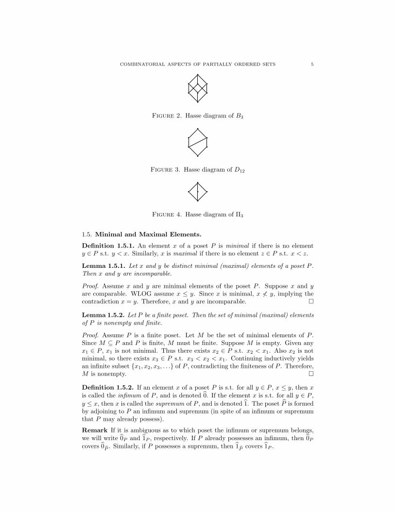
(3) Given n ∈ N, the poset Bn is the power set of [n] ordered by inclusion; i.e.,X ≤Bn

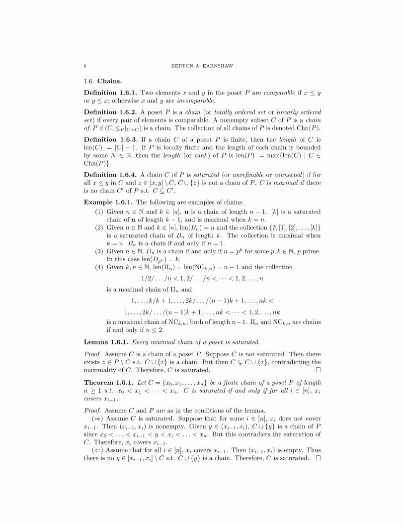
Y if and only if X ⊆ Y .(4) Given n ∈ N, the poset Dn is the set of positive divisors of n ordered by

divisibility; i.e., x ≤Dny if and only if x divides y.

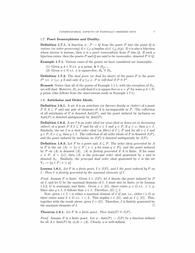
(5) Given n ∈ N, the poset Πn is the set of partitions of [n] ordered by refine-ment; i.e., π ≤Πn

σ if and only if for each A ∈ π there is B ∈ σ s.t. A ⊆ B.π is then a refinement of σ.

Definition 1.1.2. A poset P is finite if P is finite.

Remark Notice that the posets (2) through (5) from Example 1.1.1 are finite.

1.2. Subposets.

Definition 1.2.1. A weak subposet of the poset P is a poset Q s.t. Q ⊆ P andif x ≤Q y, then x ≤P y. If also Q = P , then P is a refinement of Q. Q is aninduced subposet (or subposet for short) of P if also ≤Q=≤P |Q×Q. If R ⊆ P , then(R,≤P |R×R) is the subposet induced by P (or the relation of P ) on R.

Example 1.2.1. The following are examples of subposets of the posets defined inExample 1.1.1.

(1) Given n ∈ N and k ∈ [n], k is a subposet of n.(2) Given n ∈ N and k ∈ [n], Bk is a subposet of Bn.(3) Given n ∈ N and k ∈ [n] s.t. k divides n, Dk is a subposet of Dn.(4) Given k, n ∈ N, define the poset NCk,n as the subposet of Πkn s.t each

partition π ∈ NCk,n is non-crossing (i.e., if B,B′ ∈ π and a < b < c < d s.t.a, c ∈ B and b, d ∈ B′, then B = B′) and each block of π has cardinalitydivisible by k.

Remark In the case that k = 1 from part (4) above, define NCn := NC1,n.

Theorem 1.2.1. If P is a finite poset, then there are exactly 2|P | subposets of P .

Proof. Assume the poset P is finite. Since P is finite, there are exactly 2|P | subsetsof P . Given P ′ ⊆ P , there is only one relation ≤′ s.t. (P ′,≤′) is a subposet of P ,namely ≤′=≤|P ′×P ′ . Therefore, there are exactly 2|P | subposets of P . ˜

Definition 1.2.2. If x ≤ y in the poset P , then the closed interval (or intervalfor short) from x to y, denoted ambiguously by [x, y], is the subposet inducedby P on the set [x, y] := {z ∈ P | x ≤ z ≤ y}. The open interval from xto y, denoted ambiguously by (x, y), is the subposet induced by P on the set(x, y) := {z ∈ P | x < z < y}. The collection of all intervals of P is denoted Int(P ).

Remark Notice that [x, x] = {x} and (x, x) = ∅. If it is ambiguous as to whichposet [x, y] or (x, y) is a subposet, we will write [x, y]P or (x, y)P instead.

Lemma 1.2.1. A poset P is determined by the collection Int(P ).


Proof. This follows from the fact that (P,≤P ) = ∪I∈Int(P )

(I,≤P |I×I). ˜

1.3. Locally Finite Posets.

Definition 1.3.1. A poset P is locally finite if every interval of P is finite.

Theorem 1.3.1. Every finite poset is locally finite.

Proof. Assume the poset P is finite. Suppose it is not locally finite. Then for someI ∈ Int(P ), I is not finite. But I is a subposet of P , which implies the contradictionP is not finite. Therefore, P is locally finite. ˜

Warning! The converse of this theorem is not always true! For instance, N is alocally finite, but infinite, poset.

Definition 1.3.2. If x < y and (x, y) = ∅ in the poset P , then y covers x.

Lemma 1.3.1. A finite poset is determined by its covering relations.

Proof. Assume P is a finite poset. Suppose P is not determined by its coveringrelations. Then there exist x, y ∈ P s.t. for all w, z ∈ [x, y], w does not cover z.Choose p1 ∈ (x, y). Such an element exists since y does not cover x. Since [x, p1] ⊆[x, y], [x, p1] is not determined by its cover relations. Now choose p2 ∈ (x, p1).Continuing inductively defines an infinite subset {p1, p2, p3, . . .} of P , implying thecontradiction P is infinite. Therefore, P is determined by its covering relations. ˜

Warning! An infinite poset is not always determined by its covering relations! Forinstance, [0, 1] is an interval of R with no covering relations. To see this, let x < yin [0, 1]. Since R is topologically connected, (x, y) is not empty. Thus y does notcover x. Since x and y were chosen arbitrarily, no element covers another in [0, 1].Therefore, [0, 1] is cannot be determined by its covering relations.

Theorem 1.3.2. A locally finite poset is determined by its cover relations.

Proof. Assume P is a locally finite poset. By Lemma 1.2.1, P is determined byInt(P ). Given I ∈ Int(P ), I is finite. Thus, by Lemma 1.3.1, I is determined byits covering relations. Therefore, P is determined by its covering relations. ˜

1.4. Hasse Diagrams.

Definition 1.4.1. The Hasse Diagram of a finite poset P is the graph whose vertexset is P and whose edge set is the covering relations in P . If x covers y in P , thenx is drawn with a higher horizontal coordinate than y.

Example 1.4.1. The following figures are examples of Hasse diagrams.

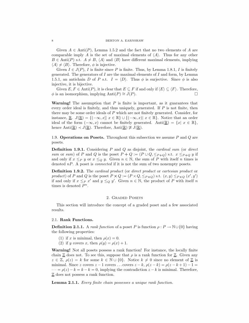
Figure 1. Hasse diagram of 3


Figure 2. Hasse diagram of B3

Figure 3. Hasse diagram of D12

Figure 4. Hasse diagram of Π3

1.5. Minimal and Maximal Elements.

Definition 1.5.1. An element x of a poset P is minimal if there is no elementy ∈ P s.t. y < x. Similarly, x is maximal if there is no element z ∈ P s.t. x < z.

Lemma 1.5.1. Let x and y be distinct minimal (maximal) elements of a poset P .Then x and y are incomparable.

Proof. Assume x and y are minimal elements of the poset P . Suppose x and yare comparable. WLOG assume x ≤ y. Since x is minimal, x 6< y, implying thecontradiction x = y. Therefore, x and y are incomparable. ˜

Lemma 1.5.2. Let P be a finite poset. Then the set of minimal (maximal) elementsof P is nonempty and finite.

Proof. Assume P is a finite poset. Let M be the set of minimal elements of P .Since M ⊆ P and P is finite, M must be finite. Suppose M is empty. Given anyx1 ∈ P , x1 is not minimal. Thus there exists x2 ∈ P s.t. x2 < x1. Also x2 is notminimal, so there exists x3 ∈ P s.t. x3 < x2 < x1. Continuing inductively yieldsan infinite subset {x1, x2, x3, . . .} of P , contradicting the finiteness of P . Therefore,M is nonempty. ˜

Definition 1.5.2. If an element x of a poset P is s.t. for all y ∈ P , x ≤ y, then xis called the infimum of P , and is denoted 0. If the element x is s.t. for all y ∈ P ,

y ≤ x, then x is called the supremum of P , and is denoted 1. The poset P is formedby adjoining to P an infimum and supremum (in spite of an infimum or supremumthat P may already possess).

Remark If it is ambiguous as to which poset the infimum or supremum belongs,we will write 0P and 1P , respectively. If P already possesses an infimum, then 0P

covers 0 bP. Similarly, if P possesses a supremum, then 1 bP

covers 1P .


1.6. Chains.

Definition 1.6.1. Two elements x and y in the poset P are comparable if x ≤ yor y ≤ x; otherwise x and y are incomparable.

Definition 1.6.2. A poset P is a chain (or totally ordered set or linearly orderedset) if every pair of elements is comparable. A nonempty subset C of P is a chainof P if (C,≤P |C×C) is a chain. The collection of all chains of P is denoted Chn(P ).

Definition 1.6.3. If a chain C of a poset P is finite, then the length of C islen(C) := |C| − 1. If P is locally finite and the length of each chain is boundedby some N ∈ N, then the length (or rank) of P is len(P ) := max{len(C) | C ∈Chn(P )}.

Definition 1.6.4. A chain C of P is saturated (or unrefinable or connected) if forall x ≤ y in C and z ∈ [x, y] \C, C ∪ {z} is not a chain of P . C is maximal if thereis no chain C′ of P s.t. C ( C′.

Example 1.6.1. The following are examples of chains.

(1) Given n ∈ N and k ∈ [n], n is a chain of length n − 1. [k] is a saturatedchain of n of length k − 1, and is maximal when k = n.

(2) Given n ∈ N and k ∈ [n], len(Bn) = n and the collection {∅, [1], [2], . . . , [k]}is a saturated chain of Bn of length k. The collection is maximal whenk = n. Bn is a chain if and only if n = 1.

(3) Given n ∈ N, Dn is a chain if and only if n = pk for some p, k ∈ N, p prime.In this case len(Dpk) = k.

(4) Given k, n ∈ N, len(Πn) = len(NCk,n) = n− 1 and the collection

1/2/ . . . /n < 1, 2/ . . . /n < · · · < 1, 2, . . . , n

is a maximal chain of Πn and

1, . . . , k/k + 1, . . . , 2k/ . . . /(n− 1)k + 1, . . . , nk <

1, . . . , 2k/ . . . /(n− 1)k + 1, . . . , nk < · · · < 1, 2, . . . , nk

is a maximal chain of NCk,n, both of length n−1. Πn and NCk,n are chainsif and only if n ≤ 2.

Lemma 1.6.1. Every maximal chain of a poset is saturated.

Proof. Assume C is a chain of a poset P . Suppose C is not saturated. Then thereexists z ∈ P \ C s.t. C ∪ {z} is a chain. But then C ( C ∪ {z}, contradicting themaximality of C. Therefore, C is saturated. ˜

Theorem 1.6.1. Let C = {x0, x1, . . . , xn} be a finite chain of a poset P of lengthn ≥ 1 s.t. x0 < x1 < · · · < xn. C is saturated if and only if for all i ∈ [n], xi

covers xi−1.

Proof. Assume C and P are as in the conditions of the lemma.(⇒) Assume C is saturated. Suppose that for some i ∈ [n], xi does not cover

xi−1. Then (xi−1, xi) is nonempty. Given y ∈ (xi−1, xi), C ∪ {y} is a chain of Psince x0 < . . . < xi−1 < y < xi < . . . < xn. But this contradicts the saturation ofC. Therefore, xi covers xi−1.

(⇐) Assume that for all i ∈ [n], xi covers xi−1. Then (xi−1, xi) is empty. Thusthere is no y ∈ [xi−1, xi] \C s.t. C ∪ {y} is a chain. Therefore, C is saturated. ˜


1.7. Poset Isomorphisms and Duality.

Definition 1.7.1. A function φ : P → Q from the poset P into the poset Q isisotone (or order-preserving) if x ≤P y implies φ(x) ≤Q φ(y). If φ is also a bijectionwhose inverse is isotone, then φ is a poset isomorphism from P into Q. If such abijection exists, then the posets P and Q are said to be isomorphic, denoted P ∼= Q.

Example 1.7.1. Various cases of the posets we have considered are isomorphic.

(1) Given p, k ∈ N s.t. p is prime, k ∼= Dpk−1 .(2) Given n ∈ N s.t. n is square-free, Bn

∼= Dn.

Definition 1.7.2. The dual poset (or dual for short) of the poset P is the posetP ∗ s.t. x ≤P∗ y if and only if y ≤P x. P is self-dual if P ∼= P ∗.

Remark Notice that all of the posets of Example 1.1.1, with the exception of Dn,are self-dual. However,Dn is self-dual if n is square-free or n = pk for some p, k ∈ N,p prime (this follows from the observations made in Example 1.7.1).

1.8. Antichains and Order Ideals.

Definition 1.8.1. A set A is an antichain (or Sperner family or clutter) of a posetP if A ⊆ P and any pair of elements of A is incomparable in P . The collectionof all antichains of P is denoted Anti(P ), and the poset induced by inclusion onAnti(P ) is denoted ambiguously by Anti(P ).

Definition 1.8.2. A set I is an order ideal (or semi-ideal or down-set or decreasingsubset) of a poset P if I ⊆ P and for all x ∈ I and y ∈ P , if y ≤ x, then y ∈ I.Similarly, the set I is a dual order ideal (or filter) if I ⊆ P and for all x ∈ I andy ∈ P , if x ≤ y, then y ∈ I. The collection of all order ideals of P is denoted J(P ),and the poset induced by inclusion on J(P ) is denoted ambiguously by J(P ).

Definition 1.8.3. Let P be a poset and A ⊆ P . The order ideal generated by Ain P is the set 〈A〉 := {x ∈ P | x ≤ y for some y ∈ P}, and the poset inducedby P on 〈A〉 is denoted 〈A〉. 〈A〉 is finitely generated if A is finite. If for somex ∈ P , A = {x}, then 〈A〉 is the principal order ideal generated by x and isdenoted Λx. Similarly, the principal dual order ideal generated by x is the setVx := {y ∈ P | x ≤ y}.

Lemma 1.8.1. Let P be a finite poset, I ∈ J(P ), and I the poset induced by P onI. Then I is finitely generated by the maximal elements of I.

Proof. Assume P is finite. Given I ∈ J(P ), let I denote the poset induced by Pon I, and let G be the maximal elements of I. I must also be finite, so by Lemma1.5.2, G is nonempty and finite. Given x ∈ 〈G〉, there exists g ∈ G s.t. x ≤ g.Since also g ∈ I, it follows that x ∈ I. Therefore, 〈G〉 ⊆ I.

Now, given i ∈ I, i is either a maximal element of I of not; i.e., either i ∈ G orthere exists some h ∈ G s.t. i < h. This implies i ∈ 〈G〉, and so I ⊆ 〈G〉. This,together with the result above, gives I = 〈G〉. Therefore, I is finitely generated bythe maximal elements of I. ˜

Theorem 1.8.1. Let P be a finite poset. Then Anti(P ) ∼= J(P ).

Proof. Assume P is a finite poset. Let φ : Anti(P ) → J(P ) be a function definedfor all A ∈ Anti(P ) by φ(A) = 〈A〉. Clearly, φ is well-defined.


Given A ∈ Anti(P ), Lemma 1.5.2 and the fact that no two elements of A arecomparable imply A is the set of maximal elements of 〈A〉. Thus for any otherB ∈ Anti(P ) s.t. A 6= B, 〈A〉 and 〈B〉 have different maximal elements, implying〈A〉 6= 〈B〉. Therefore, φ is injective.

Given I ∈ J(P ), I is finite since P is finite. Thus, by Lemma 1.8.1, I is finitelygenerated. The generators of I are the maximal elements of I and form, by Lemma1.5.1, an antichain D of P s.t. I = 〈D〉. Thus φ is surjective. Since φ is alsoinjective, it is bijective.

Given E,F ∈ Anti(P ), it is clear that E ⊆ F if and only if 〈E〉 ⊆ 〈F 〉. Therefore,φ is an isomorphism, implying Anti(P ) ∼= J(P ). ˜

Warning! The assumption that P is finite is important, as it guarantees thatevery order ideal is finitely, and thus uniquely, generated. If P is not finite, thenthere may be some order ideals of P which are not finitely generated. Consider, forinstance, R. J(R) = {(−∞, x]| x ∈ R} ∪ {(−∞, x)| x ∈ R}. Notice that an orderideal of the form (−∞, x) cannot be finitely generated. Anti(R) = {x| x ∈ R},hence Anti(R) ≺ J(R). Therefore, Anti(R) 6∼= J(R).

1.9. Operations on Posets. Throughout this subsection we assume P and Q areposets.

Definition 1.9.1. Considering P and Q as disjoint, the cardinal sum (or directsum or sum) of P and Q is the poset P + Q := (P ∪Q,≤P+Q) s.t. x ≤P+Q y ifand only if x ≤P y or x ≤Q y. Given n ∈ N, the sum of P with itself n times isdenoted nP . A poset is connected if it is not the sum of two nonempty posets.

Definition 1.9.2. The cardinal product (or direct product or cartesian product orproduct) of P and Q is the poset P ×Q := (P ×Q,≤P ˆQ) s.t. (x, y) ≤P ˆQ (x′, y′)if and only if x ≤P x′ and y ≤Q y′. Given n ∈ N, the product of P with itself ntimes is denoted Pn.

2. Graded Posets

This section will introduce the concept of a graded poset and a few associatedresults.

2.1. Rank Functions.

Definition 2.1.1. A rank function of a poset P is function ρ : P → N∪{0} havingthe following properties:

(1) if x is minimal, then ρ(x) = 0.(2) if y covers x, then ρ(y) = ρ(x) + 1.

Warning! Not all posets possess a rank function! For instance, the locally finitechain Z does not. To see this, suppose that ρ is a rank function for Z. Given anyz ∈ Z, ρ(z) = k for some k ∈ N ∪ {0}. Notice k 6= 0 since no element of Z isminimal. Since z covers z − 1 covers . . . covers z − k, ρ(z − k) = ρ(z − k+ 1)− 1 =· · · = ρ(z)− k = k− k = 0, implying the contradiction z− k is minimal. Therefore,Z does not possess a rank function.

Lemma 2.1.1. Every finite chain possesses a unique rank function.


Proof. Assume C = {x0, x1, . . . , xn} is a finite chain of length n s.t. x0 < x1 <· · · < xn. Then x0 is a minimal element of C, and for all i ∈ [n], xi covers xi−1.Define ρ : C → [0, n] by ρ(xi) = i and for all i ∈ [n]. Then ρ satisfies the propertiesof a rank function for C.

Suppose ρ′ is another rank function for C different from ρ. Then for some i ∈ [n],ρ(xi) 6= ρ′(xi). WLOG assume ρ(xi) < ρ′(xi). Then ρ′(x0) = ρ′(x1) − 1 = · · · =ρ′(xi)− i > ρ(xi)− i = i− i = 0, contradicting the fact that ρ′(x0) = 0. Therefore,ρ is unique. ˜

2.2. Graded Posets.

Definition 2.2.1. If every maximal chain of the poset P has the same lengthn ∈ N ∪ {0}, then P is graded of rank n.

Remark While the rank of a graded poset must be finite, the poset itself does notneed to be so. For instance, (N,=) is an infinite graded poset of rank 0.

Theorem 2.2.1. Every graded poset possesses a unique rank function.

Proof. Assume P is a graded poset of rank n. Let C = {x0, x1, . . . , xn} be anarbitrary maximal chain of P s.t. x0 < x1 < · · · < xn. By lemma 2.1.1 there is aunique rank function ρC : C → [0, n] for C.

Let C′ = {x′0, x′1, . . . , x

′n} be any other maximal chain s.t. x′0 < x′1 < · · · < x′n

and C ∩ C′ is nonempty. Let ρC′ be the unique rank function for C′ and supposethat for some x ∈ C ∩C′, ρC(x) 6= ρC′(x). Then for some i, j ∈ [n]∪ {0} s.t. i 6= j,x = xi = x′j . WLOG assume i < j. This implies x′0 < · · · < x′j = xi < · · · < xn

in P . But then {x′0, . . . , x′j = xi, . . . , xn} is a chain of P of length j + n − i > n,

which contradicts the fact that maximal chains in P have length n. Therefore,ρC(x) = ρC′(x), and so ρC and ρC′ agree on all of C ∩ C′.

Since P = ∪{C ⊆ P | C is a maximal chain of P},

ρ := ∪{ρC | C is a maximal chain of P}

is a rank function from P into [0, n]. The uniqueness of each ρC implies the unique-ness of ρ. ˜

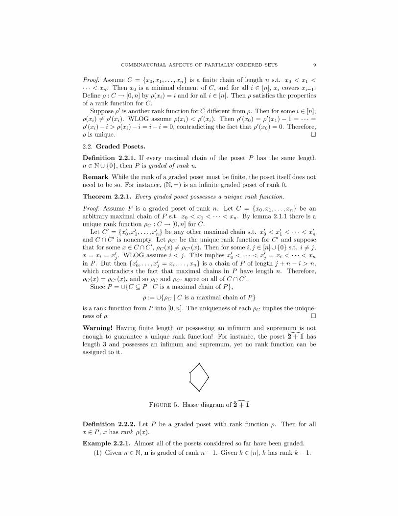
Warning! Having finite length or possessing an infimum and supremum is not

enough to guarantee a unique rank function! For instance, the poset \2 + 1 haslength 3 and possesses an infimum and supremum, yet no rank function can beassigned to it.

Figure 5. Hasse diagram of \2 + 1

Definition 2.2.2. Let P be a graded poset with rank function ρ. Then for allx ∈ P , x has rank ρ(x).

Example 2.2.1. Almost all of the posets considered so far have been graded.

(1) Given n ∈ N, n is graded of rank n− 1. Given k ∈ [n], k has rank k − 1.


(2) Given n ∈ N, Bn is graded of rank n. Given A ∈ Bn, A has rank |A|.(3) Given n ∈ N, Dn is graded of rank d(n), where d(n) is the number of prime

divisors (counting multiplicities) of n. Given k a divisor of n, k has rankd(k).

(4) Given k, n ∈ N, Πn and NCk,n are both graded of rank n − 1. Given π ineither poset, π has rank n− |π|.

Theorem 2.2.2. If x ≤ y in a graded poset P with rank function ρ, then len([x, y]) =ρ(y) − ρ(x).

Proof. Assume P is a graded poset of rank n with rank function ρ. Given x ≤ yin P , let C = {x0, x1, . . . , xn} be a maximal chain of P containing x and y s.t.x0 < x1 < · · · < xn. Then for some i, j ∈ [n] s.t. i < j, xi = x and xj = y. Thisforces len([x, y]) = j − i, else len(C) 6= n. By theorem 2.2.1, ρ(x) = i and ρ(y) = j.Therefore, len([x, y]) = j − i = ρ(y) − ρ(x) ˜

2.3. Rank-generating Function.

Definition 2.3.1. If P is a graded poset of rank n s.t. for each i ∈ [n], pi is thenumber of elements of P of rank i, then the rank-generating function of P is thefunction F(P, x) :=

∑n

i=0 pixi.

Example 2.3.1. Almost all of the posets considered so far have been graded.

(1) Given n ∈ N, the rank-generating function of n is F(n, x) =∑n−1

i=0 xi =

1 + x+ · · · + xn−1.(2) Given n ∈ N, the rank-generating function of Bn is F(Bn, x) =

∑ni=0

(ni

)xi.

(3) Given n ∈ N square-free, F(Dn, x) = F(Bn, x).(4) Given n ∈ N, the rank-generating function for Πn is

F(Πn, x) =

n−1∑

i=0

S(n, n− i)xi,

where S(n, k) = 1k!

∑k

i=0(−1)k−i(ki

)in is a Stirling number of the second

kind (ref. Section 4.1). Given k ∈ N, the rank-generating function forNCkn is

F(NCk,n, x) =

n−1∑

i=0

1

n

(n

n− i

)(kn

n− i− 1

)xi

(ref. Section 4.2).

Lemma 2.3.1. If both P and Q have finite lengths, then len(P × Q) = len(P ) +len(Q).

Proof. Assume P has length m and Q has length n. Given an arbitrary chain C ={(x0, y0), (x1, y1), . . . , (xl, yl)} of P×Q s.t. (x0, y0) <P ˆQ (x1, y1) <P ˆQ · · · <P ˆQ

(xl, yl), it follows that X = {x0, x1, . . . , xl} is a chain of P and Y = {y0, y1, . . . , yl}is a chain of Q. Notice that for each i ∈ [l], (xi−1, yi−1) <P ˆQ (xi, yi) impliesxi−1 <P xi or yi−1 <Q yi. Since len(X) ≤ m and len(Y ) ≤ n, xi−1 <P xi istrue for at most m of the i’s in [l] and yi−1 <Q yi is true for at most n of them.Therefore, len(C) = l ≤ m + n, and so every chain in the interval has length lessthan or equal to m+ n.


Let {a0, a1, . . . , am} and {b0, b1, . . . , bn} be chains of P and Q, respectively, oflengthsm and n, respectively, s.t. a0 <P a1 <P · · · <P am and b0 <P b1 <P · · · <P

bn. Then {(a0, b0), (a1, b0), . . . , (am, b0), (am, b1), . . . , (am, bn)} is a chain of P ×Qof length m + n. This result, together with the one from the previous paragraph,implies len(P ×Q) = m+ n. ˜

Theorem 2.3.1. If P is graded of rank m and Q is graded of rank n, then P ×Qis graded of rank m+ n.

Proof. Assume P and Q are graded of rankm and n, respectively. By Lemma 2.3.1,P × Q has rank m + n. Let C = {(x0, y0), (x1, y1), . . . , (xl, yl)} be an arbitrarymaximal chain of P × Q s.t (x0, y0) <P ˆQ (x1, y1) <P ˆQ · · · <P ˆQ (xl, yl). Ifl < m+ n, then the proof of Lemma 2.3.1 asserts that for some i ∈ [l], xi−1 <P xi

and yi−1 <Q yi. But this implies that C ∪ {(xi−1, yi)} is a chain of P × Q,contradicting the maximality of C. Thus len(C) = l = m + n. Since C was givenarbitrarily, P ×Q is graded of rank m+ n. ˜

Corollary 2.3.1. If both P and Q are graded, then F(P ×Q, x) = F(P, x)F(Q, x).

Proof. Assume P and Q are graded of rank m and n, respectively, with rank-generating functions F(P, x) =

∑m

i=0 pixi and F(Q, x) =

∑n

i=0 qixi, respectively.

Let x ∈ P have rank k and y ∈ Q have rank l. Let X = {x0, x1, . . . , xm} andY = {y0, y1, . . . , yn} be maximal chains of P and Q, respectively, containing x andy, respectively, s.t. x0 <P x1 <P · · · <P xm and y0 <Q y1 <Q · · · <Q yn. ByTheorem 2.2.1, x = xk and y = yl. The chain

C = {(x0, y0), . . . , (xk, y0), . . . , (xk, yl), . . . , (xk, yn), . . . , (xm, yn)}

of P ×Q s.t.

(x0, y0) < . . . < (xk, y0) < . . . < (xk, yl) < . . . < (xk, yn) < . . . < (xm, yn)

in P × Q has length m + n, and so is maximal. It follows, again by Theorem2.2.1, that (xk, yl) has rank k + l. Thus the number of elements of P × Q of rank

j is∑j

i=0 piqj−i, which is the coefficient of xj in F(P, x)F(Q, x). Therefore, therank-generating function for P ×Q is F(P ×Q, x) = F(P, x)F(Q, x). ˜

3. Lattices

This section will introduce the concept of a lattice and a few associated results,including some counting results.

3.1. Lattices. We need a few definitions before we can define a lattice.

Definition 3.1.1. Let x and y be elements of a poset P . An element z ∈ P is anupper bound of x and y if x ≤ z and y ≤ z. Let Upp(x, y) be the subposet of allupper bounds of x and y. If Upp(x, y) possesses a minimum z, then z is the join(or least upper bound) of x and y, denoted x ⌣ y, and read “x join y.”

Dually, z is a lower bound for x and y if z ≤ x and z ≤ y. Let Low(x, y) bethe subposet of all lower bounds of x and y. It Low(x, y) possesses a maximum z,then z is the meet (or greatest lower bound) of x and y, denoted x ⌢ y, and read“x meet y.”

Remark As always, we write ⌣P and ⌢P instead of ⌣ and ⌢ when it is am-biguous as to which poset the operation belongs.


Definition 3.1.2. A join-semilattice is a poset s.t every pair of elements possesesa join. A meet-semilattice is a poset s.t. every pair of elements possesses a meet.A lattice is both a join- and meet-semilattice.

Definition 3.1.3. Let L be a lattice. A sublattice of L is a subset M ⊆ L s.t. forall x, y ∈M , x ⌣ y ∈M and x ⌢ y ∈M .

Example 3.1.1. Most of the posets we have considered so far are lattices. Forinstance, given k, n ∈ N, n, Bn, Dn, Πn and NCk,n are all lattices.

Theorem 3.1.1. Let L be a lattice. Then

(1) ⌣ and ⌢ are both associative, commutative, and idempotent.(2) for all x, y ∈ L, x ⌢ (x ⌣ y) = x = x ⌣ (x ⌢ y).(3) for all x, y ∈ L, x ⌢ y = x⇔ x ⌣ y = y ⇔ x ≤ y.

Proof. Assume L is a lattice and x, y, z ∈ L. It is helpful to notice that x ≤ y ifand only if minUpp(x, y) = x and maxLow(x, y) = y.

(1) x ⌣ (y ⌣ z) ≥ x and x ⌣ (y ⌣ z) ≥ y ⌣ z. Since y ⌣ z ≥ y,x ⌣ (y ⌣ z) ≥ y. Thus x ⌣ (y ⌣ z) ≥ x ⌣ y. Also, y ⌣ z ≥ z, so x ⌣ (y ⌣z) ≥ z. Therefore, x ⌣ (y ⌣ z) ≥ (x ⌣ y) ⌣ z. A similar argument shows that(x ⌣ y) ⌣ z ≥ x ⌣ (y ⌣ z). Therefore, x ⌣ (y ⌣ z) = (x ⌣ y) ⌣ z, proving ⌣is associative in L.

Since minUpp(x, y) = minUpp(y, x), ⌣ is commutative. Since minUpp(x, x) =x, ⌣ is idempotent. Similar arguments prove ⌢ is associative in L, commutativeand idempotent.

(2) x ⌣ y ≥ x, so that x ⌢ (x ⌣ y) = x. Since x ⌢ y ≤ x, it follows thatx ⌣ (x ⌣ y) = x.

(3) If x ⌣ y = y, then x ≤ y. If x ≤ y, then x ⌢ y = x. If x ⌢ y = x, thenx ≤ y. If x ≤ y, then x ⌢ y = x. ˜

Warning! In general, joins and meets do not associate with each other! Considerthe following lattice:

0

1

x y z

xy1

Figure 6. Hasse diagram of \D2 + 1

Here, x ⌢ (y ⌣ z) = x while (x ⌢ y) ⌣ z = 1.

Lemma 3.1.1. Every nonempty finite join-semilattice (meet-semilattice) possessesa supremum (infimum).

Proof. We proceed by induction on the number of elements n ∈ N of the join-semilattice P .

(n = 1) Let P = {x}. Then 1P = x.(n = k) Suppose that, for some k ∈ N \ {1}, the statement of the lemma is true

for every join-semilattice of k elements. Let P = {x1, x2, . . . , xk+1}. The induction

hypothesis implies {x1, x2, . . . , xk} possesses a supremum 1. Then 1P = 1 ⌣ xk+1.


Thus the lemma is true for join-semilattices with k + 1 elements. Therefore, bymathematical induction, the lemma is true for every finite join-semilattice. ˜

Theorem 3.1.2. If P is a finite join-semilattice (meet-semilattice) possessing aninfimum (supremum), then P is a lattice.

Proof. Assume P is a finite join-semilattice possessing an infimum. Given x, y ∈ P ,Low(x, y) is nonempty since it contains the infimum. Thus the subposet inducedby P on Low(x, y) is nonempty and finite. It is also a join-semilattice, since for allw, z ∈ Low(x, y), w ⌣ z exists and w ⌣ z ≤ x and w ⌣ z ≤ y. Hence this inducedsubposet possesses a supremum z by Lemma 3.1.1. It follows then that x ⌢ y = z.Thus P is also a meet-semilattice, and therefore a lattice. ˜

Lemma 3.1.2. Let L and M be lattices. Then L∗, L × M and \L+M are alllattices.

Proof. Assume L and M are lattices. For all x, y ∈ L, it follows by definition thatx ⌣L y = x ⌢L∗ y and x ⌢L y = x ⌣L∗ y. Thus L∗ is a lattice.

For all (x, y), (x′, y′) ∈ L ×M , (x, y) ⌣LˆM (x′, y′) = (x ⌣L x′, y ⌣M y′) and(x, y) ⌢LˆM (x′, y′) = (x ⌢L x′, y ⌢M y′). Thus L×M is a lattice.L+M is never a lattice if both L and M are nonempty, since for all l ∈ L and

m ∈ M both Upp(l,m) and Low(l,m) are empty in L+M . In \L+M , however,

Upp(l,m) = {1} and Low(l,m) = {0}. It follows from this and the fact that L and

M are already lattices that \L+M is a lattice. ˜

3.2. Modular Lattices.

Theorem 3.2.1. Let L be a finite lattice. The following conditions are equivalent:

(1) P is a graded and for all x, y ∈ P its rank function ρ satisfies ρ(x)+ρ(y) ≥ρ(x ⌢ y) + ρ(x ⌣ y).

(2) for all x, y ∈ P , if x and y both cover x ⌢ y, then x ⌣ y covers both x andy.

Proof. Assume L is a finite lattice.(1 ⇒ 2) Assume condition (1). Let x and y be arbitrary elements of L both

covering x ⌢ y. Then ρ(x) = ρ(x ⌢ y) + 1 = ρ(y). Suppose x ⌣ y does not coverx. Then ρ(x ⌣ y) > ρ(x) + 1. Thus ρ(x ⌢ y) + ρ(x ⌣ y) > ρ(y) − 1 + ρ(x) + 1 =ρ(y) + ρ(x), contradicting condition (1). The same contradiction arises if x ⌣ ydoes not cover y. Therefore, x ⌣ y covers both x and y.

(2 ⇒ 1) Assume condition (2). Since L is finite, it has finite length n ∈ N.Suppose L is not graded. Then there exist x, y ∈ L s.t [x, y] is an ungraded intervalof L of minimal length l ≤ n.

Given any element z ∈ [x, y] covering x, [z, y] is graded since it has lengthl − 1 < l. Thus there must exist at least one other element of [x, y] covering x.If not, then every maximal chain of [x, y] is of the form C ∪ {x}, where C is amaximal chain of [z, y]. This implies every maximal chain of [x, y] has length l;i.e., the contradiction that [x, y] is graded. Also, of these other covering elements,at least one of them must form an interval with y of length different than that of[z, y]. If not, then again all the maximal chains of [x, y] are of the same length.

Therefore, let a, b ∈ [x, y] both cover x s.t. len([a, y]) 6= len([b, y]). WLOGassume len([a, y]) < len([b, y]). It follows by (2) that a ⌣ b covers both a and b.


Let B = {b, a ⌣ b, . . . , y} be a maximal chain of [b, y] (i.e., len(B) = len([b, y]))containing a ⌣ b. But then {a, a ⌣ b, . . . , y} is a chain of [a, y] of length len(B),contradicting the fact that len([a, y]) < len([b, y]). Thus [x, y], and hence L, mustbe graded. Let ρ be the rank function of L.

Now suppose condition (1)’s statement about ρ is not true. Let L′ ⊆ L be s.t.for all w, z ∈ L′, ρ(w) + ρ(z) < ρ(w ⌢ z) + ρ(w ⌣ z). Let L′′ ⊆ L′ be s.t. for allw, z ∈ L′′, len([w ⌢ z,w ⌣ z]) is minimal. From L′′ choose x and y s.t. ρ(x)+ρ(y)is minimal. If both x and y cover x ⌢ y, then condition (2) implies x ⌣ y coversboth x and y. In this case ρ(x) = ρ(y) = ρ(x ⌢ y) + 1 = ρ(x ⌣ y) − 1, so thatρ(x) + ρ(y) = ρ(x ⌢ y) + 1 + ρ(x ⌣ y) − 1 = ρ(x ⌢ y) + ρ(x ⌣ y). Thus x and ycannot both cover x ⌢ y.

WLOG assume x does not cover x ⌢ y. It follows that there exists x′ ∈(x ⌢ y, x). Our minimality assumptions imply ρ(x′)+ρ(y) ≥ ρ(x′ ⌢ y)+ρ(x′ ⌣ y).Since x < x′, x′ ⌢ y = x ⌢ y. So the above inequality becomes ρ(x′) + ρ(y) ≥ρ(x ⌢ y) + ρ(x′ ⌣ y); i.e.,

ρ(y) − ρ(x ⌢ y) ≥ ρ(x′ ⌣ y) − ρ(x′).

Our assumptions also imply ρ(x) + ρ(y) < ρ(x ⌢ y) + ρ(x ⌣ y); i.e.,

ρ(y) − ρ(x ⌢ y) < ρ(x ⌣ y) − ρ(x).

The above inequalities imply

ρ(x) + ρ(x′ ⌣ y) < ρ(x′) + ρ(x ⌣ y).

Let z = x′ ⌣ y. Since x′ ≤ x and x′ ≤ z, it follows that x′ ≤ x ⌢ z, and henceρ(x′) ≤ ρ(x ⌢ z). x ⌣ (x′ ⌣ y) = (x ⌣ x′) ⌣ y = x ⌣ y, so ρ(x ⌣ z) = ρ(x ⌣y). By choice ρ(x ⌢ y) < ρ(x′). The above inequality now says

ρ(x) + ρ(z) < ρ(x ⌢ z) + ρ(x ⌣ z)

with len([x ⌢ z, x ⌣ z]) ≤ len([x′, x ⌣ y]) < len([x ⌢ y, x ⌣ y]), contradictingthe minimality assumptions for x and y. Therefore condition (1)’s statement aboutρ is true [15, 103-104]. ˜

Definition 3.2.1. A finite lattice L is upper semimodular if it satisfies either oneof the conditions of Theorem 3.2.1. If L∗ is upper semimodular, then L is lowersemimodular. L is modular if it is both upper and lower semimodular.

Example 3.2.1. Some of the lattices considered so far are modular. For instance,given k, n ∈ N, n, Bn and Dn are modular. However, Πn and NCk,n are notmodular for n > 2.

Remark The definition of a modular lattice implies the following equivalent defi-nition: A finite lattice L is modular if and only if either of the following conditionsis true:

(1) L is graded with rank function ρ s.t for all x, y ∈ L, ρ(x) + ρ(y) = ρ(x ⌢y) + ρ(x ⌣ y).

(2) for all x, y ∈ L, x and y both cover x ⌢ y if and only if x ⌣ y covers bothx and y.

Lemma 3.2.1. The poset \2 + 1 is a nonmodular lattice.

Proof. Consider again the Hasse diagram of \2 + 1 (ref. Figure 5). \2 + 1 is a latticeby Lemma 3.1.2. It is not modular, however, since it is not graded. ˜


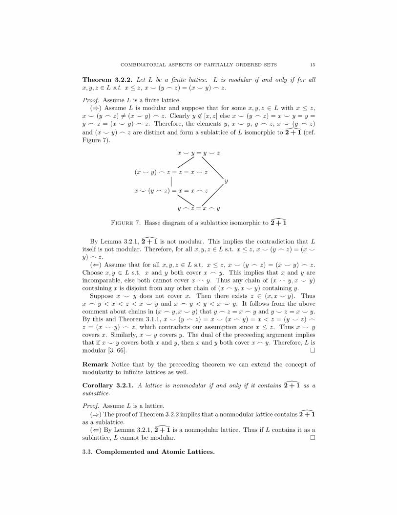
Theorem 3.2.2. Let L be a finite lattice. L is modular if and only if for allx, y, z ∈ L s.t. x ≤ z, x ⌣ (y ⌢ z) = (x ⌣ y) ⌢ z.

Proof. Assume L is a finite lattice.(⇒) Assume L is modular and suppose that for some x, y, z ∈ L with x ≤ z,

x ⌣ (y ⌢ z) 6= (x ⌣ y) ⌢ z. Clearly y 6∈ [x, z] else x ⌣ (y ⌢ z) = x ⌣ y = y =y ⌢ z = (x ⌣ y) ⌢ z. Therefore, the elements y, x ⌣ y, y ⌢ z, x ⌣ (y ⌢ z)

and (x ⌣ y) ⌢ z are distinct and form a sublattice of L isomorphic to \2 + 1 (ref.Figure 7).

y ⌢ z = x ⌢ y

x ⌣ (y ⌢ z) = x = x ⌢ z

(x ⌣ y) ⌢ z = z = x ⌣ z

y

x ⌣ y = y ⌣ z

Figure 7. Hasse diagram of a sublattice isomorphic to \2 + 1

By Lemma 3.2.1, \2 + 1 is not modular. This implies the contradiction that Litself is not modular. Therefore, for all x, y, z ∈ L s.t. x ≤ z, x ⌣ (y ⌢ z) = (x ⌣y) ⌢ z.

(⇐) Assume that for all x, y, z ∈ L s.t. x ≤ z, x ⌣ (y ⌢ z) = (x ⌣ y) ⌢ z.Choose x, y ∈ L s.t. x and y both cover x ⌢ y. This implies that x and y areincomparable, else both cannot cover x ⌢ y. Thus any chain of (x ⌢ y, x ⌣ y)containing x is disjoint from any other chain of (x ⌢ y, x ⌣ y) containing y.

Suppose x ⌣ y does not cover x. Then there exists z ∈ (x, x ⌣ y). Thusx ⌢ y < x < z < x ⌣ y and x ⌢ y < y < x ⌣ y. It follows from the abovecomment about chains in (x ⌢ y, x ⌣ y) that y ⌢ z = x ⌢ y and y ⌣ z = x ⌣ y.By this and Theorem 3.1.1, x ⌣ (y ⌢ z) = x ⌣ (x ⌢ y) = x < z = (y ⌣ z) ⌢z = (x ⌣ y) ⌢ z, which contradicts our assumption since x ≤ z. Thus x ⌣ ycovers x. Similarly, x ⌣ y covers y. The dual of the preceeding argument impliesthat if x ⌣ y covers both x and y, then x and y both cover x ⌢ y. Therefore, L ismodular [3, 66]. ˜

Remark Notice that by the preceeding theorem we can extend the concept ofmodularity to infinite lattices as well.

Corollary 3.2.1. A lattice is nonmodular if and only if it contains \2 + 1 as asublattice.

Proof. Assume L is a lattice.

(⇒) The proof of Theorem 3.2.2 implies that a nonmodular lattice contains \2 + 1

as a sublattice.(⇐) By Lemma 3.2.1, \2 + 1 is a nonmodular lattice. Thus if L contains it as a

sublattice, L cannot be modular. ˜

3.3. Complemented and Atomic Lattices.


Definition 3.3.1. Let L be a lattice with infimum and supremum. L is comple-mented if for all x ∈ L there exists y ∈ L s.t. x ⌢ y = 0 and x ⌣ y = 1. Theelement y is called a complement of x. If for all x ∈ L the complement of x is unique,then L is uniquely complemented. If every interval of L is itself complemented, thenL is relatively complemented.

Definition 3.3.2. Let L be a nonempty finite lattice. An atom of L is an elementof L covering 0, and the set of atoms of L is denoted A(L). L is atomic (or a pointlattice) if for every x ∈ L there exists a subset A ⊆ A(L) s.t. x is equal to the joinof A; i.e., if A = {a1, a2, . . . , an}, then x = a1 ⌣ a2 ⌣ · · ·⌣ an.

Dually, a coatom is an element of L covered by 1 and L is coatomic if everyelement is the meet of coatoms.

Remark Notice that 1 is the join of A(L) and, by convention, 0 is the join of ∅.

Lemma 3.3.1. Let L be an atomic lattice and a1, a2, . . . , an+1 ∈ A(L) be a finitesequence of atoms. If a1 ⌣ a2 ⌣ · · · ⌣ an and an+1 are comparable, then (a1 ⌣a2 ⌣ · · ·⌣ an) ⌣ an+1 = a1 ⌣ a2 ⌣ · · · ⌣ an. If a1 ⌣ a2 ⌣ · · ·⌣ an and an+1

are incomparable, then (a1 ⌣ a2 ⌣ · · ·⌣ an) ⌣ an+1 covers a1 ⌣ a2 ⌣ · · ·⌣ an.

Proof. Assume L is an atomic lattice and let a1, a2, . . . , an+1 ∈ A(L) be a finitesequence of atoms. For convenience, let a = a1 ⌣ a2 ⌣ · · ·⌣ an.

Suppose a and an+1 are comparable. If an+1 ≤ a, then a ⌣ an+1 = a. If

a ≤ an+1, then a = an+1 since only 0 and an+1 satisfy this relationship and a 6= 0.Thus again an+1 ≤ a so that a ⌣ an+1 = a.

Now suppose a and an+1 are incomparable. Then a < a ⌣ an+1. Since any z ∈[a, an+1] must be the join of at least {a1, a2, . . . , an} and at most {a1, a2, . . . , an+1},it follows that (a, an+1) is empty. Therefore, a ⌣ an+1 covers a. ˜

Corollary 3.3.1. Let a and an+1 be as in the previous lemma. Then a and an+1

are incomparable if and only if a ⌢ an+1 = 0.

Proof. If a and an+1 are incomparable, then a ⌢ an+1 < an+1. But the only

element of L satisfying this relationship is 0. If a and an+1 are comparable, thenit follows from the proof of the previous lemma that an+1 ≤ a. Therefore, a ⌢an+1 = an+1. ˜

3.4. Semimodular Independence and Geometric Lattices.

Theorem 3.4.1. Let L be a semimodular lattice with rank function ρ. Given anyfinite sequence x1, x2, . . . , xn ∈ L, ρ(x1 ⌣ x2 ⌣ · · ·⌣ xn) ≤ ρ(x1) + ρ(x2) + · · · +ρ(xn).

Proof. Proof by induction on the length n of the finite sequence x1, x2, . . . , xn ∈ L.Suppose n = 1. Then, trivially, ρ(x1) ≤ ρ(x1).

Suppose the statement of the theorem is true for some k ∈ N. Given any finitesequence x1, x2, . . . , xk+1 ∈ L, the semimodularity of L and the induction hypoth-esis imply ρ((x1 ⌣ x2 ⌣ · · ·⌣ xk) ⌣ xk+1)+ ρ((x1 ⌣ x2 ⌣ · · ·⌣ xk) ⌢ xk+1) ≤ρ(x1 ⌣ x2 ⌣ · · · ⌣ xk) + ρ(xk+1) ≤ ρ(x1) + ρ(x2) + · · · + ρ(xk) + ρ(xk+1); i.e.,ρ((x1 ⌣ x2 ⌣ · · ·⌣ xk) ⌣ xk+1) ≤ ρ(x1)+ρ(x2)+ · · ·+ρ(xk)+ρ(xk+1)−ρ((x1 ⌣x2 ⌣ · · · ⌣ xk) ⌢ xk+1). Since ρ((x1 ⌣ x2 ⌣ · · · ⌣ xk) ⌢ xk+1) is nonnega-tive, the statement of the theorem is true for any finite sequence of length k + 1.Therefore, by mathematical induction, the theorem is true for all finite sequencesin L. ˜


Definition 3.4.1. Let L be an upper semimodular lattice with rank function ρ.A finite sequence x1, x2, . . . , xn ∈ L is independent if ρ(x1 ⌣ x2 ⌣ · · · ⌣ xn) =ρ(x1) + ρ(x2) + · · · + ρ(xn).

Lemma 3.4.1. Let L be an atomic, upper semimodular lattice with rank functionρ. Then a1, a2, . . . , an ∈ L is independent in L if and only if for all i, j ∈ [n], ifi 6= j, then ai and aj are incomparable.

Proof. Assume L is an atomic, upper semimodular lattice with rank function ρ.Let a1, a2, . . . , an ∈ A(L) be a finite sequence of atoms.

(⇒) Suppose a1, a2, . . . , an is independent in L. Proceed by induction on n. Ifn = 1, then ρ(x1) = ρ(x1). Suppose the the statement is true for some k ∈ N.Semimodularity and independence imply k + 1 = ρ(a1 ⌣ a2 ⌣ · · · ⌣ ak+1) =ρ(a1 ⌣ a2 ⌣ · · · ⌣ ak) + ρ(ak+1) − ρ((a1 ⌣ a2 ⌣ · · · ⌣ ak) ⌢ ak+1) =k + 1 − ρ((a1 ⌣ a2 ⌣ · · · ⌣ ak) ⌢ ak+1). The induction hypothesis impliesa1, a2, . . . , ak are pairwise incomparable. If ak+1 is comparable with any elements

of a1, a2, . . . , ak, Corrolary 3.3.1 implies that (a1 ⌣ a2 ⌣ · · · ⌣ ak) ⌢ ak+1 6= 0,so that ρ((a1 ⌣ a2 ⌣ · · · ⌣ ak) ⌢ ak+1) 6= 0, contradicting the independenceof a1, a2, . . . , ak+1. Therefore, a1, a2, . . . , ak+1 are all pairwise incomparable. Thusthe statement is true when n = k + 1, and therefore, by mathematical induction,true for all independent sequences of atoms.

(⇐) Suppose the atoms a1, a2, . . . , an are all pairwise incomparable. By Lemma3.3.1, ak+1 covers a1 ⌣ a2 ⌣ · · ·⌣ ak for all k ∈ [n− 1]; i.e., ρ(a1 ⌣ a2 ⌣ · · ·⌣ak+1) = ρ(a1 ⌣ a2 ⌣ · · · ⌣ ak) + 1. It follows then that ρ(a1 ⌣ a2 ⌣ · · · ⌣an) = n = ρ(a1) + ρ(a2) + · · · + ρ(an). Therefore, the sequence a1, a2, . . . , an isindependent. ˜

Theorem 3.4.2. Let L be a finite upper semimodular lattice. The following con-ditions are equivalent:

(1) L is relatively complemented.(2) L is atomic.

Proof. Assume L is a finite upper semimodular lattice with rank function ρ.(1 ⇒ 2) Assume L is relatively complemented. Suppose L is not atomic. Choose

x ∈ L \ {0} s.t. x is not the join of atoms and ρ(x) is minimal.

By our assumptions, [0, x] is complemented. Let a be an atom of [0, x] and let c

be a complement of a in [0, x]. c 6= x, else a ≤ c so that a ⌢ c = a, contradicting thefact that c is a complement of a. Thus c < x, hence ρ(c) < ρ(x). The minimalityof ρ(x) implies that c is the join of atoms. But x = a ⌣ c, contradicting the factthat x is not equal to the join of atoms. Therefore, L is atomic.

(2 ⇒ 1) Assume L is atomic and let [x, y] be any interval of L. Let z ∈ [x, y]. ByLemma 3.4.1, we can choose a finite independent sequence of atoms a1, a2, . . . , an

that is also independent of z s.t. z ⌣ (a1 ⌣ a2 ⌣ · · · ⌣ an) = y. Let a = a1 ⌣a2 ⌣ · · · ⌣ an. Lemma 3.4.1 now implies that ρ(z ⌣ a) = ρ(z) + n, and sincex ≤ z, ρ(x ⌣ a) = ρ(x) + n.

Let c = x ⌣ a. Then z ⌣ c = z ⌣ (x ⌣ a) = (z ⌣ x) ⌣ a = z ⌣ a = y. Sincex ≤ z and x ≤ c, x ≤ z ⌢ c. Semimodularity implies ρ(z ⌢ c) ≤ ρ(z)+ρ(c)−ρ(z ⌣c) = ρ(z) + ρ(x ⌣ a) − ρ(z ⌣ a) = ρ(z) + ρ(x) + n − (ρ(z) + n) = ρ(x). Thusz ⌢ c = x, proving c is the complement of z in [x, y]. Therefore, L is relativelycomplemented [3, 105-106]. ˜


Definition 3.4.2. A finite semimodular lattice satisfying either of the conditionsof Theorem 3.4.2 is a geometric lattice.

4. Lattices of Partitions

In this section we will apply what we have learned so far to the lattice of partitionsof an n-set, Πn, and to the lattice of noncrossing partitions of a kn-set with blocksof cardinality divisble by k, NCk,n.

4.1. The Lattice of Partitions of an n-Set. Given n ∈ N, recall that Πn is theset of all partitions of the set [n], ordered by refinement; i.e., π ≤ π′ in Πn if andonly if for all B ∈ π there exists B′ ∈ π′ s.t. B ⊆ B′. When writing partitions of [n],it is sometimes convenient to seperate blocks by a slash (/) and elements in a block,written in ascending order, by comma (,). Thus the partition {{1}, {2, 3}} ∈ Π3 issometimes written 1/2, 3.

Clearly Πn is finite. It also possesses an infimum and supremum, namely 0 =1/2/ . . . /n and 1 = 1, 2, . . . , n.

Lemma 4.1.1. π′ covers π = {B1, B2, . . . , Bl} in Πn if and only if there existdistinct i, j ∈ [l] s.t. π′ = (π \ {Bi, Bj}) ∪ {Bi ∪Bj}.

Proof. (⇒) Assume π′ covers π = {B1, B2, . . . , Bl} in Πn. Suppose there does notexist distinct i, j ∈ [l] s.t. π′ = (π \ {Bi, Bj}) ∪ {Bi ∪Bj}. Since π < π′, two casesfollow:

(1) There are distinct A,B ∈ π′ and distinct a, b, c, d ∈ [l] s.t. Ba∪Bb ⊆ A andBc ∪Bd ⊆ B. But then π < (π \ {Ba, Bb})∪ {Ba ∪Bb} < π′, contradictingthe fact that (π, π′) = ∅.

(2) There are distinct A,B,C ∈ π′ s.t. for some D ∈ π, A ∪B ∪ C ⊆ D. Butthen π < (π \ {A,B}) ∪ {A ∪ B} < π′, again contradicting the fact that(π, π′) = ∅.

Since both cases contradict the fact that π′ covers π, there must exist distincti, j ∈ [l] s.t. π′ = (π \ {Bi, Bj}) ∪ {Bi ∪Bj}. ˜

Remark Notice that, in the previous theorem, |π′| = |π| − 1.

Corollary 4.1.1. Let π ≤ σ in Πn. The each block of σ is the union of blocks ofπ.

Proof. Assume π ≤ σ in Πn. If π = σ, the result is obvious. Lemma 4.1.1 impliesthe result when σ covers π. Suppose then that π is neither equal to or covered byσ. Let π = π0 < π1 < · · · < πl = σ be a saturated chain of Πn. Thus for all i ∈ [l],πi covers πi−1. By Lemma 4.1.1, each block of πi is the union of blocks of πi−1. Itthen follows by induction that each block of σ is the union of blocks of π. ˜

Theorem 4.1.1. Πn is graded of rank n− 1. If ρ is the rank function of Πn andπ ∈ Πn, then ρ(π) = n− |π|.

Proof. Let C = {π0, π1, . . . , πl} be a maximal chain of Πn s.t. π0 < π1 < · · · < πl.

Then π0 = 0 = 1/2/ . . . /n, and since for all i ∈ [l], πi covers πi−1, Lemma 4.1.1implies l = n− 1. Therefore, Πn is graded of rank n− 1.

Let ρ be the rank function of Πn. By definition, ρ(0) = 0 = n −∣∣∣0

∣∣∣. It follows

from Lemma 4.1.1 and induction that for all π ∈ Πn, ρ(π) = n− |π|. ˜


Theorem 4.1.2. For all k ∈ [0, n− 1], there are

S(n, n− k) =1

(n− k)!

n−k∑

i=0

(−1)n−k−i

(n− k

i

)in

partitions of Πn of rank k.

Proof. By definition, S(n, k), called a Stirling number of the second kind, is thenumber of partitions of an n-set into k blocks. By convention, S(0, 0) = 1. Ifk > n, then S(n, k) = 0, since there is no way to partition an n-set into morenonempty blocks than there are elements. If n ≥ 1, then the following are true:

(1) S(n, 0) = 0, since there is no way to partition an n-set into zero blocks.(2) S(n, 1) = 1, since the only such partition is 1, 2, . . . , n.(3) S(n, 2) = 2n−1 − 1. To see this, notice that this is essentially a problem

of choosing which of two indistinct bins to place each of the distinct nelements without leaving a bin empty. After we have placed n − 1 of theelements, there are two possible cases to consider:(a) One bin is empty. Then all n − 1 elements were placed in the same

bin. There is just one way of doing this, and we are then forced toplace the nth element in the other bin.

(b) Neither bin is empty. There are S(n − 1, 2) ways of doing this. Thenth element can then be placed in either of the two bins. Thus thereis a total of 2 · S(n− 1, 2) ways to place the n elements.

Thus S(n, 2) = 2·S(n−1, 2)+1. First, S(1, 2) = 0 since 2 > 1 and 21−1−1 =20 − 1 = 1− 1 = 0. If we suppose that, for some k ∈ N, S(k, 2) = 2k−1 − 1,then S(k+1, 2) = 2·S(k, 2)+1 = 2(2k−1−1)+1 = 2k−2+1 = 2(k+1)−1−1.Therefore, by mathematical induction, S(n, 2) = 2n−1 − 1.

(4) S(n, n − 1) =(n2

). To see this, notice first that all the bins must be

nonempty. So after placing all n elements, n − 2 of the bins will con-tain just one element, while the other bin will contain two elements. Thenumber of ways of doing this is just the number of ways of choosing twoelements from n; i.e,

(n2

)ways.

(5) S(n, n) = 1, since the only such partition is 1/2/ . . . /n.

In general, placing n− 1 of n distinct elements into k indistinct bins yields twocases:

(1) One bin is left empty. Thus the n− 1 elements were placed in k − 1 bins.The number of ways of doing this is S(n− 1, k− 1). The last element mustbe placed in the empty bin.

(2) No bin is left empty. Thus the n − 1 elements were place in k bins. Thenumber of ways of doing this is S(n− 1, k). The last element can then beplaced in any of the k bins. Thus this case yields a total of k · S(n− 1, k)ways to place the n elements.

Therefore, S(n, k) = k ·S(n− 1, k)+S(n− 1, k− 1). If for all k ∈ N∪{0} we define

Fk(x) :=∑∞

n=kS(n,k)

n! xn, then

Fk(x) = k

∞∑

n=k

S(n− 1, k)

n!xn +

∞∑

n=k

S(n− 1, k − 1)

n!xn.


Differentiating boths sides with respect to x gives

F ′k(x) = k

∞∑

n=k

n · S(n− 1, k)

n!xn−1 +

∞∑

n=k

n · S(n− 1, k − 1)

n!xn−1 =

k

∞∑

n=k

S(n− 1, k)

(n− 1)!xn−1 +

∞∑

n=k

S(n− 1, k − 1)

(n− 1)!xn−1 =

k∞∑

n=k

S(n, k)

n!xn +

∞∑

n=k−1

S(n, k − 1)

n!xn = kFk(x) + Fk−1(x).

Now, F0(x) =∑∞

n=0S(n,0)

n! xn = S(0, 0) +∑∞

n=1S(n,0)

n! xn = 1 +∑∞

n=10n!x

n =

1 + 0 = 1. Also, if for all k ∈ N ∪ {0} we define fk(x) := 1k! (e

x − 1)k, then

f0(x) = 10! (e

x − 1)0 = 11 · 1 = 1. Suppose that, for some k ∈ N, Fk−1(x) =

fk−1(x). Notice that we now have a nonhomogeneous ordinary differential equationF ′

k(x) − kFk(x) = Fk−1(x) = fk−1(x) = 1(k−1)! (e

x − 1)k−1. It thus has a unique

solution. Try Fk(x) = fk(x):

f ′k(x) − kfk(x) =

d

dx(

1

k!(ex − 1)k) − k

1

k!(ex − 1)k =

k

k!(ex − 1)k−1ex −

1

(k − 1)!(ex − 1)k =

1

(k − 1)!(ex − 1)k−1ex −

1

(k − 1)!(ex − 1)k−1(ex − 1) =

(1

(k − 1)!(ex − 1)k−1)(ex − (ex − 1)) = fk−1(x)(e

x − ex + 1) = fk−1(x).

Therefore, by mathematical induction, Fk(x) = 1k! (e

x − 1)k for all k ∈ N ∪ {0}.If we now write

Fk(x) =∞∑

n=k

S(n, k)

n!xn =

1

k!(ex − 1)k =

1

k!

k∑

i=0

(−1)k−i

(k

i

)eix =

1

k!

k∑

i=0

(−1)k−i

(k

i

) ∞∑

n=0

in

n!xn =

∞∑

n=0

1k!

∑k

i=0(−1)k−i(ki

)in

n!xn

and equate coefficients, we see that S(n, k) = 1k!

∑k

i=0(−1)k−i(ki

)in. Since a par-

tition π ∈ Πn of rank k = n − |π|, π has n − k blocks. Therefore, there are

S(n, n − k) = 1(n−k)!

∑n−ki=0 (−1)n−k−i

(n−k

i

)in partitions of of Πn of rank k [15,

33-34]. ˜

Corollary 4.1.2. The rank-generating function for Πn is

F(Πn, x) =

n−1∑

k=0

S(n, n− k)xk.

Proof. This follows directly from Theorem 4.1.2. ˜

Definition 4.1.1. For all n ∈ N, the number B(n) := F(Πn, 1) is called the nthBell number.

Remark Notice that the nth Bell number is equal to the cardinality of Πn.

Theorem 4.1.3. Πn is a geometric lattice.


Proof. Given π, σ ∈ Πn, let τ = {A ∩ B | A ∈ π,B ∈ σ,A ∩ B 6= ∅}. Thenτ ∈ Low(π, σ). Given υ ∈ Low(π, σ) and B ∈ υ, there exists P ∈ π and S ∈ σ s.t.B ⊆ P and B ⊆ S. Thus B ⊆ P ∩S. Hence P ∩S 6= ∅, and so P ∩S ∈ τ . It followsthen that υ ≤ τ . Thus τ is the maximal element of Low(π, σ), and so π ⌢ σ = τ .Therefore, Πn is a meet-semilattice. Since Πn possesses a supremum, it follows byTheorem 3.1.2 that Πn is a lattice.

It is obvious that Π1 and Π2 are geometric (Π1∼= 1 and Π2

∼= 2). So supposen ≥ 3 and let α, β ∈ A(Πn) be distinct atoms of Πn. It follows from Lemma 4.1.1that α contains all singleton blocks except one block A = {a, a′} which containstwo elements. The same is true for β, so call its non-singleton block B = {b, b′}.

Then A 6= B, else α = β. If A ∩B 6= ∅, then α ⌣ β = (0 \ {a, a′, b, b′}) ∪ {A ∪B}.If A ∩B = ∅, then α ⌣ β = (0 \ {a, a′, b, b′}) ∪ {A,B}. In either case, the rank ofα ⌣ β is two. Thus α ⌣ β covers both α and β.

Suppose π = {B1, B2, . . . , Bl} ∈ Πn. Define a function φ : [π, 1] → Πl for all

τ ∈ [π, 1] by φ(τ) = {I ⊆ [l] | ∃B ∈ τ s.t. B = ∪i∈IBi}. Corrolary 4.1.1 implies φ

is a well-defined isomorphism. Therefore, [π, 1] ∼= Πl.

Now let σ and τ both cover π. Then φ(σ) and φ(τ) both cover φ(π) = 0 inΠl. Thus φ(σ) ⌣ φ(τ) covers both φ(σ) and φ(τ). Thus σ ⌣ τ covers both σand τ . Therefore, Πn is upper semimodular. Corrolary 4.1.1 implies Πn is atomic.Therefore, Πn is geometric. ˜

4.2. The Lattice of Noncrossing Partitions of an n-Set. Given k, n ∈ N,recall that NCk,n is the subposet of all noncrossing partitions of Πkn, the cardinalityof whose blocks are divisble by k. Because NCk,n is a subposet of Πkn, it will adoptmany of the same attributes as Πkn. For instance, Lemma 4.1.1 and Corrolary4.1.1 clearly apply to NCk,n. NCk,n always possesses the supremum 1, 2, . . . , kn,but only NCn possesses an infimum 1/2/ . . . /n.

Theorem 4.2.1. NCk,n is graded of rank n− 1. If ρ is the rank function of NCk,n

and π ∈ NCk,n, then ρ(π) = t− |π|.

Proof. Let π0 < π1 < · · · < πl be a maximal chain of NCk,n. π0 is a minimalelement of NCk,n, and so contains n blocks, each of cardinality k. It follows byLemma 4.1.1 and induction that l = n − 1. Therefore, NCk,n is graded of rankn− 1. If ρ is the rank function of NCk,n, then again follows by Lemma 4.1.1 andinduction that for all π ∈ NCk,n, ρ(π) = n− |π|. ˜

Theorem 4.2.2. For all r ∈ [0, n−1], there are 1n

(n

n−r

)(kn

n−r−1

)partitions of NCk,n

of rank r.

Proof. We will first prove this for the case k = 1, and then generalize for all k.Given n ∈ N and b ∈ [n], define σb(n) = {s1, s2, . . . , sn} to be the finite sequence

s1 = b, s2 = b+ 1, . . . , sn−b+1 = n, sn−b+2 = 1, sn−b+3 = 2, . . . , sn = b− 1.

Given X ∈ NCn, the blocks of X can be ordered relative to σb(n) by letting B1 bethe block containing b and, for all i ∈ [2, n], letting Bi be the block containing thenumber furthest to the left in σb(n) not contained in B1 ∪B2 ∪ · · · ∪Bi−1.

Given k ∈ N∪{0}, let (L,R1, R2, . . . , Rk) ∈ (Bn\{∅})k+1 s.t. |L| = (∑k

1=1 |Ri|)+1. Parenthesize σb(n) in the following way: insert an open parenthesis to the leftof every element of σb(n) contained in L and a closed parenthesis to the rightof every element of σb(n) any time it appears in the sets R1, R2, . . . , Rk. σb(n)


parenthesized in this way is denoted σb(n), and is well-parenthesized if it begins withan open parenthesis and, with the removal of that open parenthesis, the remainingparenthesis all close. This leads to an important lemma:

Lemma 4.2.1. Let (L,R1, R2, . . . , Rk) ∈ (Bn \ {∅})k+1 s.t. |L| = (∑k

1=1 |Ri|)+ 1.Then given n ∈ N, there exists a unique b ∈ [n] s.t. σb(n) is well-parenthesized.

Proof. Assume n ∈ N. We proceed by induction on the cardinality of L. If |L| = 1,then L = {x} for some x ∈ [n]. Then k must be equal to 0, so there are no subsetsR. Therefore, b = x.

Suppose the theorem is true for some l ∈ N. Let (L,R1, R2, . . . , Rk) ∈ Bk+1n s.t.

|L| = l + 1. Choose x ∈ L and, for some i ∈ [k], y ∈ Ri s.t. the block (x, . . . , y)contains no internal parentheses. If we remove x from L and y from Ri, we geta k- or k + 1-tuple s.t. |L| = l. The induction hypothesis provides a unique bs.t. σb(n) is well-parenthesized with respect to the new tuple. Let r, t ∈ [n] s.t.sr = x and st = y with respect to σb(n). It follows from our choice of x and y((x . . . y) contained no internal parentheses) that r ≤ t. Let σb(n)′ be σb(n) withan open parenthesis to the left of x and a closed parenthesis to the right of y. Theabove discussion guarantees σb(n)′ is well-parenthesized. Therefore, b is a numbers.t. σb(n) with respect to (L,R1, R2, . . . , Rk) is well-parenthesized. Suppose b′ isanother number s.t. σb′(n) with respect to (L,R1, R2, . . . , Rk) is well-parenthesized,then the removal of x and y again implies b′ = b [2]. ˜

σb(n) is associated with a noncrossing partition of Πn as follows. Add a rightparenthesis to at the end of σb(n). If a substring of σb(n) is enclosed by paren-theses and contains no internal parentheses, then remove the substring and theparentheses and call that a block. Then perform the same procedure on the newstring. Continue this until the string is empty. The well-parenthesizedness of σb(n)ensures that the chosen blocks will form a partition of [n]. The way we chose theblocks guarantees the partition is noncrossing.

Define, by the previous lemma, a function φ from all pairs (L,R) ∈ B2n s.t.

|L| = |R|+ 1 = k into all pairs (X, b) ∈ NCn × [n] s.t. X has k blocks. The lemmaguarantees that φ is injective. Given (X, b) ∈ NCn× [n], order the blocks of X withrespect to σb, and then order the elements of each block as they appear in σb. LetL be the first elements of these blocks, and R the last elements of all but the firstblock. Therefore, φ is surjective, and so bijective.

There are(nk

)(n

k−1

)such pairs (L,R). Since this number is equal to the number

of such pairs (X, b) times n, we see that the number of noncrossing partitions of[n] with k blocks is 1

n

(nk

)(n

k−1

). Since a noncrossing partition of [n] with k has rank

n− k, it follows that there are 1n

(n

n−k

)(n

n−k−1

)noncrossing partitions of [n] of rank

k [6, 172-173].For the generalization, refer to [6, 175-176]. ˜

Theorem 4.2.3. The rank-generating function for NCk,n is

F(NCk,n, x) =n−1∑

i=0

1

n

(n

n− i

)(kn

n− i− 1

)xi

Proof. This follows immediately from Theorem 4.2.2. ˜

Remark Note that∑n−1

i=01n

(n

n−i

)(n

n−i−1

)=

∑ni=1

1n

(ni

)(n

i−1

)= 1

n+1

(2nn

)= Cn, the

nth Catalan number. Thus Cn = F(NCn, 1)


Remark Since, for all k 6= 1, NCk,n is finite and does not possess an infimum, itfollows that NCk,n is not a lattice. However, given n ∈ N, NCn does possess aninfimum. In fact, NCn is a lattice, called the lattice of noncrossing partitions of ann-set.

Theorem 4.2.4. NCn is a geometric sublattice of Πn.

Proof. Given π, σ ∈ NCn, let τ = {A ∩ B | A ∈ π,B ∈ σ,A ∩ B 6= ∅}. Clearlyτ is noncrossing, since a crossing in τ would cause a crossing in π or σ. Henceτ ∈ Low(π, σ). Given υ ∈ Low(π, σ) and B ∈ υ, there exists P ∈ π and S ∈ σ s.t.B ⊆ P and B ⊆ S. Thus B ⊆ P ∩S. Hence P ∩S 6= ∅, and so P ∩S ∈ τ . It followsthen that υ ≤ τ . Thus τ is the maximal element of Low(π, σ), and so π ⌢ σ = τ .Therefore, NCn is a meet-semilattice. Since NCn possesses a supremum, it followsby Theorem 3.1.2 that NCn is a lattice.

It is obvious that NC1 and NC2 are geometric (NC1∼= Π1 and NC2

∼= Π2).So suppose n ≥ 3 and let α, β ∈ A(NCn) be distinct atoms of NCn. It followsfrom Lemma 4.1.1 that α contains all singleton blocks except one block A = {a, a′}which contains two elements. The same is true for β, so call its non-singletonblock B = {b, b′}. Then A 6= B, else α = β. If A ∩ B 6= ∅, then α ⌣ β =

(0 \ {a, a′, b, b′})∪ {A∪B}. If A∩B = ∅, then α ⌣ β = (0 \ {a, a′, b, b′})∪ {A,B}.In either case, the rank of α ⌣ β is two. Thus α ⌣ β covers both α and β.

Suppose π = {B1, B2, . . . , Bl} ∈ NCn. Define a function φ : [π, 1] → NCl for all

τ ∈ [π, 1] by φ(τ) = {I ⊆ [l] | ∃B ∈ τ s.t. B = ∪i∈IBi}. Corrolary 4.1.1 implies φ

is a well-defined isomorphism. Therefore, [π, 1] ∼= NCl.

Now let σ and τ both cover π. Then φ(σ) and φ(τ) both cover φ(π) = 0 in NCl.Thus φ(σ) ⌣ φ(τ) covers both φ(σ) and φ(τ), implying σ ⌣ τ covers both σ andτ . Therefore, NCn is upper semimodular. Corrolary 4.1.1 implies NCn is atomic.Therefore, NCn is geometric. Since NCn is atomic, it follows that NCn is closedunder joins and meets. Therefore, NCn is a sublattice of Πn. ˜

4.3. Meanders as a subposet of NCn × NC∗n. By Theorem 4.2.4 and Lemma

3.1.2, NCn × NC∗n is a lattice. It can be shown that NCn is self-dual [14, 196-

197]. Thus NC∗n must be geometric as well. Clearly the product of two geometric

lattices is again a geometric lattice. Thus NCn × NC∗n is a geometric lattice. By

Corrolary 2.3.1, F(NCn × NC∗n, x) = F(NCn, x)F(NC∗

n, x) = [F(NCn, x)]2 since

NCn is self-dual. Therefore, F(NCn × NC∗n, x) = [

∑n−1i=0

1n

(n

n−i

)(n

n−i−1

)xi]2 =

2(n−1)∑

i=0

[ i∑

j=0

1

n

(n

n− j

)(n

n− j − 1

)1

n

(n

n− (i− j)

)(n

n− (i− j) − 1

)]xi =

2(n−1)∑

i=0

[ 1

n2

i∑

j=0

(n

n− j

)(n

n− j − 1

)(n

n− i+ j

)(n

n− i+ j − 1

)]xi

so that there are 1n2

∑i

j=0

(n

n−j

)(n

n−j−1

)(n

n−i+j

)(n

n−i+j−1

)elements of NCn × NC∗

n

of rank i.An element P := (P+, P−) ∈ NCn ×NC∗

n is connected if the graph of P , denotedΓP , is connected [8, 9-10]. Any element of NCn × NC∗

n is a system of closedmeanders of order n, and any connected element of NCn ×NC∗

n is a closed meander(or meander for short) of order n [8, 10-11]. We denote the lattice of systems of


meanders by Sn (i.e., Sn∼= NCn × NC∗

n) and the subposet of Sn of all meanders oforder n by Mn.

Little is known about Mn. It is known that Mn is a graded [8, 13-15], self-dual[7] poset. Unfortunately, Mn is not a lattice for n ≥ 4, which has made deriving itsrank-generating function a centuries-old problem.

5. Distributive Lattices

We now consider a class of lattices of the upmost combinatorial importance.

5.1. Distributive Lattices.

Definition 5.1.1. Let L be a lattice. L is distributive if ⌣ and ⌢ distribute overeach other; i.e., for all x, y, z ∈ L

(1) x ⌣ (y ⌢ z) = (x ⌣ y) ⌢ (x ⌣ z).(2) x ⌢ (y ⌣ z) = (x ⌢ y) ⌣ (x ⌢ z).

Theorem 5.1.1. Every lattice satisfying condition 1 or 2 of Definition 5.1.1 isdistributive.

Proof. Assume L is a lattice. Suppose L satisfies condition 1 of Definition 5.1.1.Given x, y, z ∈ L, condition 1 and Theorem 3.1.1 imply (x ⌢ y) ⌣ (x ⌢ z) =((x ⌢ y) ⌣ x) ⌢ ((x ⌢ y) ⌣ z) = x ⌢ ((x ⌣ z) ⌢ (y ⌣ z)) = (x ⌢ (x ⌣ z)) ⌢(y ⌣ z) = x ⌢ (y ⌣ z); i.e., condition 2 of Definition 5.1.1 is true. Therefore, L isdistributive.

Now suppose L is a lattice satisfying condition 2. Then condition 2 and Theorem3.1.1 imply (x ⌣ y) ⌢ (x ⌣ z) = ((x ⌣ y) ⌢ x) ⌣ ((x ⌣ y) ⌢ z) = x ⌣ ((x ⌢z) ⌣ (y ⌢ z)) = (x ⌣ (x ⌢ z)) ⌣ (y ⌢ z) = x ⌣ (y ⌢ z); i.e., condition 1 istrue. Therefore, L is distributive. ˜

Theorem 5.1.2. Every distributive lattice is modular.

Proof. Assume L is a distributive lattice. Given x, y, z ∈ L s.t. x ≤ z, it followsthat x ⌣ z = z. Thus x ⌣ (y ⌢ z) = (x ⌣ y) ⌢ (x ⌣ z) = (x ⌣ y) ⌢ z.Therefore, by Theorem 3.2.2, L is modular. ˜

Example 5.1.1. Some of the lattices we have consider thus far are distributive.For instance, given k, n ∈ N, n, Bn and Dn are distributive. However, Example3.2.1 states Πn and NCk,n are not modular for n > 2, hence they can not bedistributive for the same n.

5.2. The Fundamental Theorem of Finite Distributive Lattices. Recallthat for any poset P , J(P ) is the poset of all order ideals of P ordered by in-clusion.

Theorem 5.2.1. Let P be a poset. Then J(P ) is a distributive lattice.

Proof. Assume P is a poset. In J(P ), let joins and meets correspond to set unionsand intersections, respectively. Given I, J ∈ J(P ), let A and B be generators for Iand J , respectively. Then I ∪ J = 〈A〉 ∪ 〈B〉 = 〈A ∪B〉 ∈ J(P ) and I ∩ J = 〈A〉 ∩〈B〉 = 〈A ∩ B〉 ∈ J(P ). Thus J(P ) is a lattice. Since set unions and intersectionsdistribute over each other, it follows that J(P ) is a distributive lattice. ˜


Definition 5.2.1. An element x of a lattice L is join-irreducible if whenever y, z ∈L and x = y ⌣ z, then x = y or x = z. The set of all join-irreducibles of P isdenoted J (P ), while the subposet induced on J (P ) by P is ambiguously denotedby J (P ). Dually, x is meet-irreducible if whenever y, z ∈ L and x = y ⌢ z, thenx = y or x = z.

Theorem 5.2.2. Let P be a finite poset. I ∈ J(P ) is join-irreducible if and onlyif I is a principal order ideal.

Proof. Assume P is a finite poset and I ∈ J(P ) is arbitrary.(⇒) Suppose I is join-irreducible. Since P is finite, I is finitely generated. Let

A ⊆ P be the set of generators of I. Suppose |A| > 1. Choose a ∈ A and letB = {a}. Then 〈A \ B〉 ∪ 〈B〉 = 〈A〉 = I, contradicting the fact that I is join-irreducible. Therefore, |A| = 1, proving I is a principal order ideal.

(⇐) Suppose I is a principal order ideal. Then there exists some x ∈ L s.t.I = Λx. Let J,K ∈ J(P ) s.t. J ∪ K = I. Let B ⊆ P generate J and C ⊆ Pgenerate K. Then B ∪ C = {x}. Thus B ⊆ {x}. Since B is nonempty, B = {x}.Therefore, J = I, proving I is join-irreducible. ˜

Corollary 5.2.1. Let P be a finite poset. Then P ∼= J (J(P )).

Proof. Assume P is a finite poset. Theorem 5.2.2 implies that the function φ : P →J (J(P )), defined for all x ∈ P by φ(x) = Λx, is a bijection. Since x ≤ y if andonly if Λx ⊆ Λy, it follows that φ is also isotone. Therefore, φ is an isomorphism,proving P ∼= J (J(P )). ˜

Lemma 5.2.1. Let P and Q be finite posets. Then J(P ) ∼= J(Q) if and only ifP ∼= Q.

Proof. Assume P and Q are finite posets.(⇒) Suppose J(P ) ∼= J(Q). Since J (J(P )) and J (J(Q)) are subposets of J(P )

and J(Q), respectively, it follows that J (J(P )) ∼= J (J(Q)). Corrolary 5.2.1 thenimplies P ∼= Q.

(⇐) Suppose P ∼= Q. Corrolary 5.2.1 implies J (J(P )) ∼= J (J(Q)). Since everyorder ideal I is the join of a finite collection of principal order ideals, it follows thatJ(P ) ∼= J(Q). ˜

Theorem 5.2.3 (Fundamental Theorem of Finite Distributive Lattices). Let L bea finite distributive lattice. Then there exists a unique (up to isomorphism) finiteposet P for which L ∼= J(P ).

Proof. Assume L is a finite distributive lattice. For each x ∈ L, define Ix := {y ∈J (L) | y ≤ x}, considered as a subposet of J (L). Notice Ix ∈ J(J (L)) since ify ∈ Ix and z ≤ y in L, then z ≤ y ≤ x in L; i.e., z ∈ Ix. Define a functionφ : L→ J(J (L)) for all x ∈ L by φ(x) = Ix. Clearly, φ is well-defined.

Suppose that for x, y ∈ L, Ix 6= Iy. Then Ix \ Iy 6= ∅ or Iy \ Ix 6= ∅. AssumeWLOG that there exists z ∈ Ix \ Iy . Then z ≤ x but z 6≤ y. This implies x 6= y.Thus φ is injective.

Given I ∈ J(J (L)), let j be the join of I. Notice that I ⊆ Ij and j is the joinof Ij ; i.e.,

⌣i∈I

i = j = ⌣i∈Ix

i.


Let w ∈ Ix. It follows by distributivity that

⌣i∈I

(i ⌢ w) = (⌣i∈I

i) ⌢ w = ( ⌣i∈Ix

i) ⌢ w = ⌣i∈Ix

(i ⌢ w).

The right-hand side of the above equation is just w since w ∈ Ix. That meansone of the join-ands is w ⌣ w = w and the rest are ≤ w. Thus

⌣i∈I

(i ⌢ w) = w

and since w is join-irreducible, there must be some i ∈ I s.t. i ⌣ w = w; i.e., w ≤ i.Since I is an order ideal and i ∈ I, it follows that w ∈ I. Thus Ix ⊆ I, provingI = Ix. Therefore, φ is surjective, and thus bijective.

It is clear that x ≤ y if and only if Ix ⊆ Iy . Thus φ is isotone. This, togetherwith the bijectivity of φ implies φ is an isomorphism. Therefore, L ∼= J(J (L)).

Suppose that P is a poset s.t. J(P ) ∼= L. Lemma 5.2.1 implies then thatP ∼= J (L), proving the uniqueness (up to isomorphism) of J (L) [15, 106]. ˜

5.3. The Rank of a Finite Distributive Lattice.

Lemma 5.3.1. Let I ∈ J(P ) be an arbitrary order ideal. Then I ′ ∈ J(P ) covers Iif and only if for some minimal element x of P \ I, I ′ = I ∪ {x}.

Proof. Assume I is an arbitrary order ideal of J(P ).(⇒) Suppose I ′ ∈ J(P ) covers I. Let M = I ′ \ I. Notice M ∈ J(P ). Let x ∈M

be a minimal element of M . This implies that x is also a minimal element of P \ I.If M 6= {x}, then I ∪ {x} ∈ (I, I ′), contradicting the fact that I ′ covers I. ThusM = {x} and I ′ = I ∪ {x}.

(⇐) Suppose I ′ = I ∪ {x}, where x is a minimal element of P . Then I ′ ∈ J(P ).Clearly (I, I ′) = ∅. Since I ⊆ I ′, I ′ covers I. ˜

Theorem 5.3.1. If |P | = n, then J(P ) is graded of rank n. If ρ is the rankfunction of J(P ) and I ∈ J(P ), then ρ(I) = |I|.

Proof. Assume |P | = n. By Theorem 5.1.2, we know J(P ) is modular, and thusgraded. Let ρ be the rank function of J(P ).

Notice ∅ is the infimum of J(P ). Then ρ(∅) = 0 = |∅|. Since P is nonempty andfinite, we can choose a minimal element from P and call it x1. Then {x1} ∈ J(P )and covers ∅ in J(P ) by Lemma 5.3.1. Thus ρ({x1}) = 1 = |{x1}|.

Suppose that for some k ∈ [n−1] we have chosen elements x1, x2, . . . , xk ∈ P s.t.for all i ∈ [k−1], {x1, x2, . . . , xi+1} covers {x1, x2, . . . , xi} in J(P ) and for all j ∈ [k],ρ({x1, x2, . . . , xj}) = |{x1, x2, . . . , xj}| = j. Since P \ {x1, x2, . . . , xk} is nonemptyand finite, it contains a minimal element xk+1. Lemma 5.3.1 implies then that{x1, x2, . . . , xk+1} covers {x1, x2, . . . , xk} in J(P ). Thus ρ({x1, x2, . . . , xk+1}) =ρ({x1, x2, . . . , xk}) + 1 = |{x1, x2, . . . , xk}| = k + 1 = |{x1, x2, . . . , xk+1}|.

It follows by mathematical induction that a maximal chain of J(P ) has lengthn. Therefore, J(P ) is graded of rank n. It also follows that for all I ∈ J(P ),ρ(I) = |I|. ˜

Corollary 5.3.1. Given n ∈ N, let Pn be the collection of all isomorphism classesof n-element posets and Dn the collection of all isomorphism classes of finite dis-tributive lattices of rank n. Then |Pn| = |Dn|.


Proof. Define φ : Pn → Dn for all [P ] ∈ Pn by φ([P ]) = [J(P )]. Theorem 5.3.1assures that the domain and range are appropriate, and Lemma 5.2.1 implies that φis well-defined. If we define ψ : Dn → Pn for all [J(P )] by ψ([J(P )]) = [J (J(P ))],then ψ is the inverse of φ since, by Theorem 5.2.2, J (J(P )) ∼= P . Therefore, φ isa bijection, proving |Pn| = |Dn|. ˜

Definition 5.3.1. Given n ∈ N, the poset Bn is a boolean algebra.

Theorem 5.3.2. Let L be a finite distributive lattice. The following conditions ofL are equivalent:

(1) L is a boolean algebra,(2) L is complemented,(3) L is relatively complemented,(4) L is atomic,

(5) 1 is the join of atoms of L,(6) L is geometric,

(7) every join-irreducible of L covers 0,(8) if |J (L)| = n, then |L| = 2n,(9) for some n ∈ N, F(L, x) = (1 + x)n.

Proof. Left to the interested reader (and not the slothful author). ˜

5.4. Chains of a Finite Distributive Lattice.

Theorem 5.4.1. Let m ∈ N. The following quantities are equal:

(1) the number of surjective isotone functions from P into m.

(2) the number of chains of J(P ) of length m containing 0 = ∅ and 1 = P .

Proof. Assume m ∈ N. Let Σ be the collection of surjective isotone maps fromP into m and χ the collection of chains of J(P ) of length m containing ∅ and P .Define a function φ : Σ → χ for all σ ∈ Σ by φ(σ) = {σ−1(0), σ−1(1), . . . , σ−1(m)}(here we employ the convention that 0 = ∅).

Notice that, for all i ∈ [0,m], σ−1(i) is an order ideal of P . This follows fromthe fact that σ is isotone, for if y ≤P x, then σ(y) ≤m σ(x), implying y ∈ σ−1(i) ifx ∈ σ−1(i). Also, σ−1(0) = ∅ and σ−1(m) = P , so that φ(σ) contains both ∅ andP .

If j ∈ [0,m] s.t. i 6= j, then σ−1(i) 6= σ−1(j) since σ surjective. WLOG, assumei < j. Then σ−1(i) ( σ−1(j). Thus φ(σ) ∈ χ, proving φ is well-defined.

Let τ ∈ Σ s.t. φ(σ) = φ(τ). Then for each i ∈ [m], σ−1(i) \ σ−1(i − 1) =τ−1(i)\τ−1(i − 1); i.e., σ−1(i) and τ−1(i). Therefore, σ = τ , proving φ is injective.

Let {I0, I1, . . . , Im} ∈ χ s.t. ∅ = I0 <J(P ) I1 <J(P ) · · · <J(P ) Im = P . Defineυ : P → [m] as follows: for all i ∈ [m] and x ∈ Ii \ Ii−1, υ(x) := i. Notice σ issurjective and isotone, and thus σ ∈ Σ. Also, for all i ∈ [0,m], υ−1(i) = Ii. Thusφ(υ) = {I0, I1, . . . , Im}, proving φ is surjective. Therefore, φ is bijective, proving|Σ| = |χ| [15, 110]. ˜

Definition 5.4.1. Let |P | = n. Then any surjective, isotone function σ : P → n

is a linear extension of P (or extension of P to a total order). The number of suchfunctions is denoted e(P ).

Corollary 5.4.1. e(P ) is equal to the number of maximal chains of J(P ).


Proof. Theorem 5.3.1 implies that if |P | = n, then J(P ) is graded of rank n. Itfollows then from Theorem 5.4.1 that the number of chains of J(P ) of length n(i.e., the the number of maximal chains of J(P )) is equal to the number of linearextensions of P . This number is e(P ). ˜

Remark Stanley claims [15, 110] that e(P ) is “probably the single most usefulnumber for measuring the ‘complexity’ of P .”

6. A Useful Algebra Review

The following is a useful review of some of the algebraic structures and theorieswe will need.

6.1. Rings, Fields and R-Algebras. We review some definitions and resultsfrom ring theory.

Definition 6.1.1. A ring is an ordered triple (R,+, ·), denoted ambiguously byR, consisting of a set R and two binary opeartions + and · (called addition andmultiplication, respectively) on R satisfying the following three properties:

(1) (R,+) is an abelian group (the additive identity is denoted 0).(2) multiplication is associative; i.e., for all a, b, c ∈ R, (a · b) · c = a · (b · c).(3) multiplication is right and left distributive over addition; i.e., for all a, b, c ∈

R, (a+ b) · c = (a · c) + (b · c) and a · (b+ c) = (a · b) + (a · c).

The ring R is commutative if multiplication is commutative; i.e., for all a, b ∈ R,a · b = b · a. R is said to have an identity (or contain a 1) if there is an element1 ∈ R s.t. for all a ∈ R, 1 · a = a · 1 = a.

Remark Since (R,+) is a group, every r ∈ R will possess a unique additive inverse,denoted −r. If it is ambiguous as to which ring +, ·, 0 or 1 belong, we write instead+R, ·R, 0R or 1R, respectively.

Lemma 6.1.1. If R is a ring, then for all r ∈ R, r · 0 = 0 · r = 0.

Proof. Assume R is a ring. Given r ∈ R, r · 0 = r · (0 + 0) = (r · 0)+ (r · 0). Adding−(r · 0) to both sides yields r · 0 = 0. Similarly, 0 · r = 0. ˜

Definition 6.1.2. A ring homomorphism from a ring R into a ring A is a functionϕ : R → A s.t. for all a, b ∈ R, ϕ(a+ b) = ϕ(a) + ϕ(b) and ϕ(a · b) = ϕ(a) · ϕ(b). Ifϕ is also a bijection, then ϕ is a ring isomorphism, and R and A are isomorphic,denoted R ∼= A.

Remark When it is understood that ϕ is a homomorphism of rings, we will simplycall ϕ a homomorphism.

Warning! A homomorphism ϕ : R → A from a ring R into a ring A does notnecessarily map 1R to 1A. For instance, ϕ could send every element of R to 0A.This is indeed a homomorphism since for all r, s ∈ R, 0A = ϕ(r+s) = ϕ(r)+ϕ(s) =0A + 0A = 0A and 0A = ϕ(r · s) = ϕ(r) · ϕ(s) = 0A · 0A = 0A.

Lemma 6.1.2. Let ϕ : R → A be a homomorphism from a ring R into a ring A.Then ϕ(0R) = 0A and for all r ∈ R, ϕ(−r) = −ϕ(r).

Proof. Assume ϕ : R → A is a homomorphism from a ring R into a ring A. Thenϕ(0R) = ϕ(0R + 0R) = ϕ(0R) + ϕ(0R). Therefore, ϕ(0R) = 0A. Hence for anyr ∈ R, 0A = ϕ(0R) = ϕ(r + (−r)) = ϕ(r) + ϕ(−r). Therefore, −ϕ(r) = ϕ(−r). ˜


Definition 6.1.3. A subring of a ring R is a subgroup of R that is closed undermultiplication.

Theorem 6.1.1. Let ϕ : R→ A be a homomorphism from a ring R into a ring A.Then ϕ(R) is a subring of A.

Proof. Assume ϕ : R → A is a homomorphism from a ring R into a ring A. Givenx, y ∈ ϕ(R), there exist a, b ∈ R s.t. ϕ(a) = x and ϕ(b) = y. It follows by Lemma6.1.2 that x + (−y) = ϕ(a) + (−ϕ(b)) = ϕ(a) + ϕ(−b) = ϕ(a + (−b)) ∈ ϕ(R).Thus ϕ(R) is closed under addition and inverses, and hence a subgroup of A. Also,x · y = ϕ(a) · ϕ(b) = ϕ(a · b) ∈ ϕ(R), so ϕ(R) is also closed under multiplication.Therefore, ϕ(R) is a subring of A. ˜

Definition 6.1.4. A ring R with identity 1 6= 0 is a division ring (or skew field)if every nonzero element has a multiplicative inverse; i.e., for all r ∈ R there existsr′ ∈ R s.t. r · r′ = r′ · r = 1. A commutative division ring is a field.

Lemma 6.1.3. The multiplicative inverse of any element of a division ring isunique.

Proof. Assume R is a division ring. Given r ∈ R, let s, t ∈ R both be multiplicativeinverses of r. Then, by defintion, r · s = 1 = r · t. Let x be either s or t. Thenx · (r · s) = (x · r) · s = 1 · s = s and x · (r · t) = (x · r) · t = 1 · t = t. Therefore, s = t,so that the multiplicative inverse of r is unique. ˜

Remark The multiplicative inverse of an element r in a division ring R is denotedr−1.

Theorem 6.1.2. Let ϕ : R → A be a homomorphism from a division ring R intoa ring A with identity s.t ϕ(1R) = 1A. Then ϕ is injective.

Proof. Assume ϕ : R → A is a homomorphism from a field R into a ring A s.tϕ(1R) = 1A. Suppose there exists some r ∈ R \ {0R} s.t. ϕ(r) = 0A. This implies1A = ϕ(1R) = ϕ(r · r−1) = ϕ(r) · ϕ(r−1) = 0A · ϕ(r−1) = 0A, a contradiction sinceR is a division ring. Thus r = 0R.

Now, given s, t ∈ R, suppose ϕ(s) = ϕ(t). Then 0A = ϕ(s) + (−ϕ(t)) = ϕ(s) +ϕ(−t) = ϕ(s+(−t)). The above result implies s+(−t) = 0A; i.e., s = t. Therefore,ϕ is injective. ˜

Definition 6.1.5. The center of a ring R is the set Z(R) := {z ∈ R | ∀r ∈ R, z ·r =r·z}; i.e., the set of elements of R that commute multiplicatively with every elementof R.

Definition 6.1.6. Let R be a commutative ring with identity. An R-algebra is anordered pair (A,ϕ) consisting of a ring A with identity and a ring homomorphismϕ : R → A s.t. ϕ(1R) = 1A and ϕ(R) ⊆ Z(A).

Corollary 6.1.1. Let R be a division ring and (A,ϕ) an R-algebra. Then R ∼=ϕ(R) and R is field.

Proof. Assume R is a division ring and (A,ϕ) is an R-algebra. By Theorem 6.1.2,ϕ is injective. Thus R ∼= ϕ(R), so that ϕ(R) is a division ring. Since ϕ(R) ⊆ Z(A),ϕ(R) is commutative division ring; i.e., ϕ(R) is a field. Therefore, R is a field. ˜


Remark In the case above, we say that A is an algebra over R. It is the same assaying that A contains the field R in its center and the identity of R and A are thesame.

6.2. Modules and Vector Spaces. We review the definitions of a module and avector space and give an example of a vector space we will use in the next section.

Definition 6.2.1. Let R be a ring. A left R-module (or a left module over R) isan ordered triple (V,⊕,⊙), ambiguously denoted V , consisting of a set V and twooperations ⊕ and ⊙ satisfying the following properties:

(1) (V,⊕) is an abelian group.(2) ⊙ : R×V → V , where for all (r, v) ∈ R×V , r⊙ v := ⊙((r, v)), is an action

of R on V which satisfies:(a) for all r, s ∈ R and v ∈ V , (r · s) ⊙ v = r ⊙ (s⊙ v).(b) for all r, s ∈ R and v ∈ V , (r + s) ⊙ v = (r ⊙ v) ⊕ (s⊙ v).(c) for all r ∈ R and v, w ∈ V , r ⊙ (v ⊕ w) = (r ⊙ v) ⊕ (r ⊙ w).(d) if R has an identity, then for all v ∈ V , 1R ⊙ v = v, (in which case V

is sometimes called a unital left R-module).

A right R-module (or a right module over R) is defined analogously.

Remark If R is commutative, then a left R-module V can be made into a rightR-module by defining r ⊙ v = v ⊙ r for all r ∈ R and v ∈ V .

Definition 6.2.2. A module over R is a vector space if R is a field.

Theorem 6.2.1. Let K be a field, S be a set, and V the collection of all functionsfrom S into K. For all f, g ∈ V , s ∈ S and k ∈ K, define (f ⊕ g)(s) := f(s) + g(s)and (f ⊙ g)(s) := f(s) · g(s). Then (V,⊕,⊙) is a vector space over K.

Proof. Assume K, S, V , ⊕ and ⊙ are as in the conditions of the theorem. Letf, g, h be arbitrary functions in V and s ∈ S be an arbitrary element of S. Weprove first that (V,⊕) is a group.

(1) (V is closed under ⊕) Since K is closed under addition, (f ⊕g)(s) = f(s)+g(s) ∈ K, so that V is closed under ⊕.

(2) (⊕ is associative) Since addition in K is associative, [(f ⊕ g) ⊕ h](s) =(f ⊕ g)(s) + h(s) = (f(s) + g(s)) + h(s) = f(s) + (g(s) + h(s)) = f(s) +(g ⊕ h)(s) = [f ⊕ (g ⊕ h)](s). So ⊕ is associative.

(3) (V has an identity) Let 0V denote the function sending every element of Sto 0K . Then (f ⊕0V )(s) = f(s)+0V (s) = f(s)+0K = f(s) = 0K + f(s) =0V (s) + f(s) = (0V ⊕ f)(s). Thus 0V is an identity for V under ⊕.

(4) (V is close under inverses) Let −f be the function in V that sends everyelement of S to the additive inverse of f evaluated at the element. Then(f ⊕ (−f))(s) = f(s) + (−f(s)) = 0K = 0V (s). Thus −f is the ⊕-inverseof f .

Therefore, (V,⊕) is a group. Since (K,+) is an abelian group, (f ⊕ g)(s) = f(s) +g(s) = g(s) + f(s) = (g ⊕ f)(s). Therefore, (V,⊕) is an abelian group.

Let k, l ∈ K be arbitrary elements of K. Since multiplication in K is associative,[(k · l)⊙ f ](s) = (k · l) · f(s) = k · (l · f(s)) = k · (l ⊙ f)(s) = [k ⊙ (l⊙ f)](s). Sincemultiplication is right distributive, [(k + l)⊙ f ](s) = (k + l) · f(s) = (k · f(s)) + (l ·f(s)) = (k ⊙ f)(s) + (l⊙ f)(s) = [(k ⊙ f) ⊕ (l⊙ f)](s). Since multiplication is alsoleft distributive, [k⊙ (l⊕ f)](s) = k · (l⊕ f)(s) = k · (l+ f(s)) = (k · l)+ (k · f(s)) =


(k · l) + (k ⊙ f)(s) = [(k · l) ⊕ (k ⊙ f)](s). Also, [1K ⊙ f ](s) = 1K · f(s) = f(s).Therefore, (V,⊕,⊙) is a vector space over K. ˜

6.3. Tensor Products.

Definition 6.3.1. Let R be a ring. A left (right) R-module V is free on thesubset S ⊆ V if for all v ∈ V \ {0V } there exist n ∈ N and unique elementsr1, r2, . . . , rn ∈ R \ {0R} and unique elements s1, s2, . . . , sn ∈ S s.t. v =

∑n

i=0 risi

(∑n

i=0 siri).

Remark It can be shown [5, 335-336] that a free R-module on the set S is unique,up to isomorphism.

Definition 6.3.2. Let S be a set. The free abelian group on S is the free Z-moduleover S.

Definition 6.3.3. Let R be a ring, V a left R-module, W a right R-module andG the free abelian group on the set V ×W . Let H be the subgroup of G generatedby all elements of the forms:

(1) (v + v′, w) − (v, w) − (v′, w),(2) (v, w + w′) − (v, w) − (v, w′),(3) (vr, w) − (v, rw).

The quotient groupG/H is the tensor product of V andW overR, denoted V ⊗RW .The cosets of V ⊗RW are called tensors and, given v ∈ V and w ∈W , v⊗w denotesthe tensor of V ⊗R W containing (v, w).

7. The Incidence Algebra of a Locally Finite Poset

In this section we introduce an algebraic structure for locally finite posets thatis useful in answering many of the combinatorial questions associated with suchposet.

7.1. The Incidence Algebra. Throughout this section we assume that P is alocally finite poset and K is a field of characteristic zero.

Definition 7.1.1. Let V (Int(P ),K) denote the vector space of all functions fromInt(P ) into K. Define convolution, denoted ∗, for all functions f, g ∈ V (Int(P ),K)and [x, y] ∈ Int(P ) by (f ∗ g)([x, y]) :=

∑x≤z≤y f([x, z]) · g([z, y]).

Remark Notice that since P is locally finite, the number of summands in theabove sum is finite. Therefore, convolution is well-defined. For all f ∈ I(P )K andk ∈ N, denote the convolution of f with itself k times by fk.

Theorem 7.1.1. (V (Int(P ),K),⊕, ∗) is an algebra over K.

Proof. Theorem 6.2.1 implies that (V,⊕) is an abelian group. Let f, g, h ∈ V (Int(P ),K)and [x, y] ∈ Int(P ) be arbitrary.

(1) (convolution is associative) Since the number of summands is finite,

[(f ∗ g) ∗ h]([x, y]) =∑

x≤z≤y

(f ∗ g)([x, z]) · h([z, y]) =

∑

x≤z≤y

[∑

x≤w≤z

f([x,w]) · g([w, z])] · h([z, y]) =


∑

x≤w≤y

f([x,w]) · [∑

w≤z≤y

g([w, z]) · h([z, y])] =

∑

x≤w≤y

f([x,w]) · (h ∗ g)([w, y]) = [f ∗ (g ∗ h)]([x, y]).

(2) (convolution is left distributive) Since multiplication in K is left distribu-tive,

[f ∗ (g ⊕ h)]([x, y]) =∑

x≤z≤y

f([x, z]) · (g ⊕ h)([z, y]) =

∑

x≤z≤y

f([x, z]) · [g([z, y]) + h([z, y])] =

∑

x≤z≤y

[f([x, z]) · g([z, y])] + [f([x, z]) · h([z, y])] =

∑

x≤z≤y

[f([x, z]) · g([z, y])] +∑

x≤z≤y

[f([x, z]) · h([z, y])] =

(f ∗ g)([x, y]) + (f ∗ h)([x, y]) = [(f ∗ g) ⊕ (f ∗ h)]([x, y]).

(3) (convolution is right distributive) Since multiplication in K is right dis-tributive,

[(g ⊕ h) ∗ f ]([x, y]) =∑

x≤z≤y

(g ⊕ h)([x, z]) · f([z, y]) =

∑

x≤z≤y

[g([x, z]) + h([x, z])] · f([z, y]) =

∑

x≤z≤y

[g([x, z]) · f([z, y])] + [h([x, z]) · f([z, y])] =

∑

x≤z≤y

[g([x, z]) · f([z, y])] +∑

x≤z≤y

[h([x, z]) · f([z, y])] =

(g ∗ f)([x, y]) + (h ∗ f)([x, y]) = [(g ∗ f) ⊕ (h ∗ f)]([x, y]).

(4) (convolution identity) Let δ ∈ V (Int(P ),K) be defined for all [x, y] ∈ Int(P )by

δ([x, y]) :=

{1, if x = y,

0, if x 6= y.

Then (f ∗ δ)([x, y]) =∑

x≤y≤z f([x, z]) · δ([z, y]) = f([x, y]). Also, (δ ∗

f)([x, y]) =∑

x≤y≤z δ([x, z])·f([z, y]) = f([x, y]). Therefore, δ is an identity

for V (Int(P ),K) under convolution.

Therefore, (V (Int(P ),K),⊕, ∗) is a ring with identity.Let ϕ : K → V (Int(P ),K) be defined for all k ∈ K by ϕ(k) := δk := k⊙δ. Given

k, l ∈ K, ϕ(k + l) = δk+l = (k + l) ⊙ δ = (k ⊙ δ) ⊕ (l ⊙ δ) = δk ⊕ δl = ϕ(k) ⊕ ϕ(l).Also, ϕ(k · l) = δk·l = (k · l) ⊙ δ = (k ⊙ δ) ∗ (l ⊙ δ) = δk ∗ δl = ϕ(k) ∗ ϕ(l). Thus ϕis a ring homomorphism.

Since multiplication in K is commutative, it follows from the above that δk ∗δl = (k · l) ⊙ δ = (l · k) ⊙ δ = δl ∗ δk, so that ϕ(K) ⊆ Z(V (Int(P ),K)). Sinceδ1K

= 1K ⊙ δ = δ, ϕ maps 1K to 1V (Int(P ),K). Therefore, (V (Int(P ),K), ϕ) is aK-algebra. Since K is a field, V (Int(P ),K) is an algebra over K. ˜


Definition 7.1.2. Let P be a locally finite poset and K a field. The incidencealgebra of P over K, denoted I(P,K), is the algebra (V (Int(P ),K),⊕, ∗) over K.

Remark For our current purposes it will suffice to let K = C, in which case wedefine I(P ) := I(P,C).

Theorem 7.1.2. Let f ∈ I(P ). The following conditions are equivalent:

(1) f has a left inverse,(2) f has a right inverse,(3) f has a two-sided inverse,(4) for all x ∈ P , f([x, x]) 6= 0.

If f has any inverse, then it is the unique two-sided inverse of f .

Proof. Assume f ∈ I(P ).(1 ⇔ 4) Suppose g ∈ I(P ) is a left inverse of f ; i.e., g ∗ f = δ. This is true if

and only if

g([x, y]) =

{f([x, x])−1, if x = y

−f([y, y])−1[∑

x≤z<y g([x, z])f([z, y])], if x < y.

(The second case is due to the fact that (g ∗ f)([x, y]) =∑

x≤z<y g([x, z]f([z, y]) +

g([x, y])f([y, y])). Thus g exists if and only if for all x ∈ P , f([x, x]) 6= 0.(2 ⇔ 4) Suppose h ∈ I(P ) is a right inverse of f . Similar to the above argument,

h([x, y]) =

{f([x, x])−1, if x = y

−f([x, x])−1[∑

x<z≤y f([x, z])h([z, y])], if x < y,

so that h exists if and only if for all x ∈ P , f([x, x]) 6= 0.(3 ⇔ 4) A two-sided inverse is necessarily a left and right inverse. Thus this

result follows from the previous arguments.Suppose that g is a left inverses of f . Then the theorem implies the existence of

a right inverse h. Hence g ∗ f = δ = f ∗ h. The theorem also provides a two-sidedinverse f ′ of f . Then g = g ∗ δ = g ∗ (f ∗ f ′) = (g ∗ f) ∗ f ′ = δ ∗ f ′ = f ′ = f ′ ∗ δ =f ′ ∗ (f ∗ h) = (f ′ ∗ f) ∗ h = δ ∗ h = h. Therefore, g = f ′ = h, proving that anyinverse is two-sided and unique [15, 114]. ˜

7.2. Some Functions of the Incidence Algebra. Throughout this subsectionwe will assume P is a locally finite poset. Of all the functions contained in I(P ),there are a few of particular interest.

7.2.1. Delta Function. We have already encountered the delta function δ, definedfor all [x, y] ∈ Int(P ) be

δ([x, y]) :=

{1 if x = y,

0 if x < y.

Recall that δ is the identity in I(P ). Also recall that δz = z ⊙ δ for all k ∈ C.

7.2.2. Zeta and Chain Functions. Another is the zeta function ζ. It is defined forall [x, y] ∈ Int(P ) by ζ([x, y]) := 1. Then for all [x, y] ∈ Int(P ), ζ2([x, y]) =∑

x≤z≤y ζ([x, z]) · ζ([z, y]) =∑

x≤z≤y 1 · 1 =∑

x≤z≤y 1 = |[x, y]|. Therefore,

ζ2([x, y]) counts the numbers of elements in [x, y].


Notice that

(ζ − δ)([x, y]) :=

{1 − 1 = 0 if x = y,

1 − 0 = 1 if x < y.

Therefore, (ζ−δ)2([x, y]) =∑

x≤z≤y(ζ−δ)([x, z])·(ζ−δ)([z, y]) =∑

x<z<y ζ([x, z])·

ζ([z, y]) =∑

x<z<y 1, which is equal to the number of chains of [x, y] of length 2.

By induction it follows that (ζ − δ)k([x, y]) counts the number of chains of [x, y] oflength k. Thus η := ζ − δ is the chain function.

A sequence of functions f1, f2, f3, . . . of I(P ) converges to a function f ∈ I(P )if for all [x, y] ∈ Int(P ) there exists N ∈ N s.t. for all n ≥ N , fn([x, y]) = f([x, y]).This defines a topology on I(P ). Now consider

(δ2 − ζ)([x, y]) :=

{2 − 1 = 1 if x = y,

0 − 1 = −1 if x < y.

By Theorem 7.1.2, δ2 − ζ has an inverse: (δ2 − ζ)−1 = (δ − (ζ − δ))−1 =∑∞

k=0 ηk,

which is valid because∑∞

k=0 ηk converges in I(P ) for all [x, y] ∈ Int(P ). Therefore,

because of our interpretation of η above, (δ2 − ζ)−1([x, y]) counts the total numberof chains of [x, y] [15, 115].

7.2.3. Lambda and Cover Functions. Yet another important function in I(P ) is thelambda function λ defined for all [x, y] ∈ Int(P ) by

λ([x, y]) :=

{1 if x = y or y covers x,

0 else.

Notice then that

(λ− δ)([x, y]) =

{1 if y covers x,

0 else.

Thus κ := λ − δ is the cover function. Notice that κ2([x, y]) =∑

x≤z≤y κ([x, z]) ·κ([z, y]). Since κ([x, z]) · κ([z, y]) 6= 0 only when y covers z covers x; i.e., x < y < zis a saturated chain. Since [x, y] is finite, this is the same as requiring x < y < zto be a maximal chain. Therefore, κ2([x, y]) counts the number of maximal chainsof [x, y] of length 2. By induction it follows that κk([x, y]) counts the number ofmaximal chains of [x, y] of length k.

Now consider

(δ − κ)([x, y]) :=

1 − 0 = 1 if x = y,

0 − 1 = −1 if y covers x,

0 − 0 = 0 else.

By Theorem 7.1.2, δ−κ has an inverse: (δ−κ)−1 =∑∞

k=0 κk, which is valid because∑∞

k=0 κk converges in I(P ) for all [x, y] ∈ Int(P ). By our interpretation of κ above,

(δ − κ)([x, y]) counts the total number of maximal chains of [x, y].

7.2.4. Mobius Function. By Theorem 7.1.2, ζ possesses an inverse in I(P ). TheMobius function µ := ζ−1. The relation µ ∗ ζ = δ is equivalent to the followingrecursive defintion of µ for all [x, y] ∈ Int(P ):

µ([x, y]) :=

{1 if x = y,

−∑

x≤z<y µ([x, z]) if x < y,


since (µ ∗ ζ)([x, y]) =∑

x≤z≤y µ([x, z]) · ζ([z, y]) =∑

x≤z≤y µ([x, z]) · 1 =

∑

x≤z<y

µ([x, z]) + µ([x, y]) = δ([x, y]).

We will see in the next subsection that µ plays an important role in the algebraI(P ).

7.3. Mobius Inversion Formula. Throughout this section, assume P is a locallyfinite poset and let CP denote the set of all functions from P into C.

Theorem 7.3.1 (Mobius Inversion Formula). Let every principal order ideal of Pbe finite. Then for all f, g ∈ CP and x ∈ P , g(x) =

∑y∈Λx

f(y) if and only if

f(x) =∑

y∈Λxg(y)µ([y, x]).

Proof. Assume that every principal order ideal of P is finite. Then the summationsin the statement of the theorem are finite, and so well-defined.

Notice that CP is a vector space on which I(P ) acts on the right as an algebra oflinear transformations by (fφ)(x) =

∑y∈Λx

f(y) · φ([x, y]), for all φ ∈ I(P ). Thusthe statement of the theorem is simply an observation in linear algebra that fζ = gif and only if f = gµ [15, 116]. ˜

Remark Of course, this theorem did not depend on C in the least. Thus theMobius Inversion Formula is still true when the incidence algebra is I(P,K) forsome field K of characteristic zero, and KP is the set of all functions from P intoK. It should also be clear that the dual statement of the theorem, requiring finiteprincipal dual order ideals and noticing that I(P ) acts on the left as an algebra oflinear transformations of CP , is true [15, 116-117].

8. A Useful Algebraic Topology Review

The following is a brief review of some of concepts of algebraic topology we willneed.

8.1. Simplicial Complexes and Order Complexes.

Definition 8.1.1. Let V be a set. A simplicial complex ∆ is a collection of subsetsof V s.t.:

(1) for all v ∈ V , {v} ∈ ∆,(2) for all F ∈ ∆, if F ′ ⊆ F , then F ′ ∈ ∆.

The elements of V are called vertices and V is called the vertex set. The elementsof ∆ are called faces. We require ∅ ∈ ∆ unless ∆ = ∅. The dimension of F ∈ ∆ isthe number dim(F ) := |F | − 1 and the dimension of ∆ is the number dim(∆) :=max{dim(F ) | F ∈ ∆}.

Definition 8.1.2. Let P be a poset. The order complex of P , denoted ∆(P ), isthe simplicial complex whose vertex set is P and whose faces are the chains of P .

9. Computing the Mobius Function

We will explain a few techniques for computing the Mobius function.


9.1. The Product Formula.

Theorem 9.1.1. Let P and Q be posets. Then I(P ×Q) = I(P ) ⊗C I(Q).

Proof. See [5, 348-349] for proof. ˜

Corollary 9.1.1 (The Product Formula). If [(x, y), (x′, y′)] ∈ Int(P × Q), thenµP ˆQ([(x, y), (x′, y′)]) = µP ([x, x′])µQ([y, y′]).

Proof. This follows directly from Theorem 9.1.1 ˜

9.2. The Reduced Euler Characteristic. Throughout this subsection assumeP is a locally finite poset.

Definition 9.2.1. Let ∆ be a simplicial complex and let fk be the number offaces of ∆ of dimension k. The reduced Euler characteristic is the number χ(∆) :=∑∞

k=−1(−1)kfk = −f−1 + f0 − f1 + f2 − · · · .

Theorem 9.2.1. Let [x, y] ∈ Int(P ) and let ck denote the number of chains fromx to y of length k. Then µ([x, y]) =

∑∞k=0(−1)kck = c0 − c1 + c2 − c3 + · · · .

Proof. Notice that µ = ζ−1 = (δ + (ζ − δ))−1 = (δ + κ)−1 = (δ − (−κ))−1 =∑∞k=0(−κ)

k =∑∞

k=0(−1)kκk. Given [x, y] ∈ Int(P ), it follows that µ([x, y]) =∑∞k=0(−1)kκk([x, y]) =

∑∞k=0(−1)kck. ˜

Corollary 9.2.1. Let [x, y] ∈ Int(P ). Then µP ([x, y]) = µP∗([y, x]).

Proof. The statement of Theorem 9.2.1 is self-dual. ˜

Theorem 9.2.2. Let [x, y] ∈ Int(P ) s.t. (x, y) is not empty. Then µ([x, y]) =χ(∆((x, y))).

Proof. Assume [x, y] ∈ Int(P ) s.t. (x, y) 6= ∅. Let ck be the number of chains fromx to y of length k and fk be the number of faces of ∆((x, y)) of dimension k. Noticethen that c0 = 0, c1 = 1, and f−1 = 1 (f−1 counts the empty set). Given k ≥ 2,ck = fk−2 since a chain x = x0 < x1 < · · · < xk = y of length k contains the facex1 < x2 < · · · < xk−1 of dimension k − 2. Therefore,

∑∞k=0 ck =

∑∞k=−1 fk; i.e.,

µ([x, y]) = χ(∆((x, y))). ˜

9.3. Homological Interpretations. Recall that for any given simplicial complex∆, one associates a topological space with ∆, called the geometric realization of ∆,denoted |∆|. The reduced Euler characteristic is classically defined by the formula

χ(|∆|) =∑

p(−1)prank(Hp(|∆|,Z)). By definition, χ(∆) = χ(|∆|). Therefore,

if (x, y) is not empty, then µ([x, y]) depends only on the geometric realization|∆((x, y))| of ∆((x, y)).

10. Other Enumerative Techniques

In this section we explain other enumerative techniques and tools built on thetheory of the previous sections.


10.1. Zeta Polynomial. Throughout this subsection, let P be a finite poset.

Definition 10.1.1. A multichain of length n of P is a sequence x1 ≤ x2 ≤ · · · ≤ xn

of elements of P .

Definition 10.1.2. For n ≥ 2, define Z(P, n) to be the number of multichains oflength n − 1 of P . Regarded as a function of n, Z(P, n) is the zeta polynomial ofP .

Lemma 10.1.1. Z(P, 2) = |P |.

Proof. This is obvious from the definition of Z(P, n), since Z(P, 2) counts the num-ber of multichains of length 1; i.e., the number of elements of P . ˜

Lemma 10.1.2. For each i ≥ 2, let bi be the number of chains of P of length i−1.Then Z(P, n) =

∑i≥2 bi

(n−2i−2

).

Proof. The number of multichains of length n− 1 having a chain of length i− 1 assupport is equal to

((i−1

n−1−(i−1)

)). ˜

References

[1] Martin Aigner. Combinatorial theory. Springer-Verlag, Berlin, 1979.[2] George M. Bergman. Terms and cyclic permutations. Algebra Universalis, 8(1):129–130, 1977.[3] Garrett Birkhoff. Lattice Theory. American Mathematical Society, New York, N. Y., 1948.[4] Peter Crawley and Robert P. Dilworth. Algebraic Theory of Lattices. Prentice Hall, Inc.,

Englewood Cliffs, N. J., 1973.[5] David S. Dummit and Richard M. Foote. Abstract Algebra. John Wiley & Sons Inc., New

York, second edition, 1999.[6] Paul H. Edelman. Chain enumeration and noncrossing partitions. Discrete Math., 31(2):171–

180, 1980.[7] Reinhard O. W. Franz. On the structure of the partially ordered set of meanders. Preprint,

1998.[8] Reinhard O. W. Franz. A partial order for the set of meanders. Ann. Comb., 2(1):7–18, 1998.[9] George Gratzer. Lattice theory. First concepts and distributive lattices. W. H. Freeman and

Co., San Francisco, Calif., 1971.[10] Thomas W. Hungerford. Algebra. Springer-Verlag, New York, 1980. Reprint of the 1974 orig-

inal.[11] Charles Richard Francis Maunder. Algebraic topology. Van Nostrand Reinhold Company,

London, 1970.[12] James R. Munkres. Topology: a first course. Prentice-Hall Inc., Englewood Cliffs, N.J., 1975.

[13] James R. Munkres. Elements of algebraic topology. Addison-Wesley Publishing Company,Menlo Park, CA, 1984.

[14] Rodica Simion and Daniel Ullman. On the structure of the lattice of noncrossing partitions.Discrete Math., 98(3):193–206, 1991.

[15] Richard P. Stanley. Enumerative combinatorics. Vol. 1. Cambridge University Press, Cam-bridge, 1997. With a foreword by Gian-Carlo Rota, Corrected reprint of the 1986 original.

Berton A. Earnshaw, College of Engineering and Technology, Brigham Young Uni-

versity, Provo, UT 84602 U.S.A.

E-mail address: [email protected]

Documents

Contents · Poset Isomorphisms and Duality 7 1.8. Antichains and Order Ideals 7 1.9. Operations on Posets 8 2. Graded Posets 8 2.1. Rank Functions 8 2.2. Graded Posets 9 ... The Lattice