Embed Size (px)
Citation preview
Nested Antichains for WS1S
Tomas Fiedor1,2 Lukas Holık2
1Red Hat, Czech Republic
Ondrej Lengal2 Tomas Vojnar2
2Brno University of Technology, Czech Republic
AVM’15

WS1S
weak monadic second-order logic of one successorI second-order⇒ quantification over relations;I monadic⇒ relations are unary (i.e. sets);I weak⇒ sets are finite;I of one successor⇒ reasoning about linear structures.
corresponds to finite automata [Buchi’60]
decidable
— but NONELEMENTARYI constructive proof via translation to finite automata
T. Fiedor Nested Antichains for WS1S AVM’15 2 / 17

WS1S
weak monadic second-order logic of one successorI second-order⇒ quantification over relations;I monadic⇒ relations are unary (i.e. sets);I weak⇒ sets are finite;I of one successor⇒ reasoning about linear structures.
corresponds to finite automata [Buchi’60]
decidable — but NONELEMENTARYI constructive proof via translation to finite automata
T. Fiedor Nested Antichains for WS1S AVM’15 2 / 17

Application of WS1S
allows one to define rich invariants
famous decision procedure: the MONA toolI often efficient (in practice)
used in tools for checking structural invariantsI Pointer Assertion Logic Engine (PALE)I STRucture ANd Data (STRAND)
many other applicationsI program and protocol verifications, linguistics, theorem provers . . .
but sometimes the complexity strikes backI unavoidable in generalI however, we try to push the usability border further
• using the recent advancements in non-deterministic automata
T. Fiedor Nested Antichains for WS1S AVM’15 3 / 17

WS1S
Syntax:I term ψ ::= X ⊆ Y | Sing(X ) | X = {0} | X = σ(Y )I formula ϕ ::= ψ | ϕ ∧ ϕ | ϕ ∨ ϕ | ¬ϕ | ∃X .ϕ
Interpretation: over finite subsets of NI models of formulae = assignments of sets to variables
sets can be encoded as binary strings:
I {1,4,5} →Index:Membership:Encoding:
012345xXxxXX
010011,
0123456xXxxXXx0100110
or01234567xXxxXXxx01001100
. . .
for each variable we have one track in the alphabetI e.g.
[00
]is symbol
Example: {X1 7→ ∅,X2 7→ {4,2}} |= ϕdef⇔ X1:
X2:
[00
][00
][01
][00
][01
]∈ L(Aϕ)
T. Fiedor Nested Antichains for WS1S AVM’15 4 / 17

Deciding WS1S using deterministic automataexample of base automaton for X = σ(Y )
0 1 2
X:Y:
[00
]X:Y:
[01
]X:Y:
[10
] X:Y:
[00
]
Example:
¬(X ⊆ Y ) ∧ ∃Z .Sing(Z ) ∨ ∃W .W = σ(Z )
A1
project W
A2 ∪ A4
A2
project Z
A6 ∩ A7
A3
complementA6
A7
A4
T. Fiedor Nested Antichains for WS1S AVM’15 5 / 17

Deciding WS1S using deterministic automataexample of base automaton for X = σ(Y )
0 1 2
X:Y:
[00
]X:Y:
[01
]X:Y:
[10
] X:Y:
[00
]
Example:
¬(X ⊆ Y ) ∧ ∃Z .Sing(Z ) ∨ ∃W .W = σ(Z )
A1
project W
A2 ∪ A4
A2
project Z
A6 ∩ A7
A3
complementA6
A7
A4
T. Fiedor Nested Antichains for WS1S AVM’15 5 / 17

Deciding WS1S using deterministic automataexample of base automaton for X = σ(Y )
0 1 2
X:Y:
[00
]X:Y:
[01
]X:Y:
[10
] X:Y:
[00
]
Example:
¬(X ⊆ Y ) ∧ ∃Z .Sing(Z ) ∨ ∃W .W = σ(Z )
A1
project W
A2 ∪ A4
A2
project Z
A6 ∩ A7
A3
complementA6
A7
A4
T. Fiedor Nested Antichains for WS1S AVM’15 5 / 17

Deciding WS1S using deterministic automataexample of base automaton for X = σ(Y )
0 1 2
X:Y:
[00
]X:Y:
[01
]X:Y:
[10
] X:Y:
[00
]
Example:
¬(X ⊆ Y ) ∧ ∃Z .Sing(Z ) ∨ ∃W .W = σ(Z )
A1
project W
A2 ∪ A4
A2
project Z
A6 ∩ A7
A3
complementA6
A7
A4
T. Fiedor Nested Antichains for WS1S AVM’15 5 / 17

Deciding WS1S using deterministic automataexample of base automaton for X = σ(Y )
0 1 2
X:Y:
[00
]X:Y:
[01
]X:Y:
[10
] X:Y:
[00
]
Example:
¬(X ⊆ Y ) ∧ ∃Z .Sing(Z ) ∨ ∃W .W = σ(Z )
A1
project W
A2 ∪ A4
A2
project Z
A6 ∩ A7
A3
complementA6
A7
A4
T. Fiedor Nested Antichains for WS1S AVM’15 5 / 17

Deciding WS1S using deterministic automataexample of base automaton for X = σ(Y )
0 1 2
X:Y:
[00
]X:Y:
[01
]X:Y:
[10
] X:Y:
[00
]
Example:
¬(X ⊆ Y ) ∧ ∃Z .Sing(Z ) ∨ ∃W .W = σ(Z )
A1
project W
A2 ∪ A4
A2
project Z
A6 ∩ A7
A3
complementA6
A7
A4
T. Fiedor Nested Antichains for WS1S AVM’15 5 / 17

Deciding WS1S using deterministic automataexample of base automaton for X = σ(Y )
0 1 2
X:Y:
[00
]X:Y:
[01
]X:Y:
[10
] X:Y:
[00
]
Example:
¬(X ⊆ Y ) ∧ ∃Z .Sing(Z ) ∨ ∃W .W = σ(Z )
A1
project W
A2 ∪ A4
A2
project Z
A6 ∩ A7
A3
complementA6
A7
A4
T. Fiedor Nested Antichains for WS1S AVM’15 5 / 17

How to handle quantification
issue with projection (existential quantification)I after removing of the tracks not all models would be acceptedI so we need to adjust the final states
1 2 3
X:Y:
[01
]X:Y:
[00
]X:Y:
[10
] X:Y:
[00
]
AX=σ(Y )
1 2 3
X:Y:
[01
]X:Y:
[00
]X:Y:
[10
] X:Y:
[00
]
→ Projection
1 2 3Y: [1]
Y: [0]
Y: [0]
Y: [0]
→ Adjust statesto accept models:
1, 01, 001, . . .
T. Fiedor Nested Antichains for WS1S AVM’15 6 / 17

Deciding WS1S using non-deterministic automata
we consider only formulae in Prenex Normal Form (∃PNF)I we focus on dealing with prefix and alternations of quantifications
based on number of alternations m
ϕ = ¬∃Xm ¬. . .¬∃X2 ¬∃X1 : ϕ0(X)︸ ︷︷ ︸ϕ1
. ..︸ ︷︷ ︸
ϕm
(1)
→ hierarchical family of automata defined as follows:I Aϕ0 = by composition of atomic automata (previously described)
I Aϕm = (22···2
Q0︸ ︷︷ ︸m
,∆m, Im,Fm)
T. Fiedor Nested Antichains for WS1S AVM’15 7 / 17

The intuition behind the procedure
Key observation for ground formulaeϕ |= iff Im ∩ Fm 6= ∅
Why?I eventually the symbols degenerate to empty ones . . .
1 2 3Y: [1]
Y: [0]
Y: [0]
Y: [0]
A∃X .X=σ(Y )
1 2 3
→ Projection
1 2 3[]
[]
[]
[]
A∃Y ,X .X=σ(Y )
T. Fiedor Nested Antichains for WS1S AVM’15 8 / 17

The intuition behind the procedure
Key observation for ground formulaeϕ |= iff Im ∩ Fm 6= ∅
Why?I eventually the symbols degenerate to empty ones . . .
1 2 3Y: [1]
Y: [0]
Y: [0]
Y: [0]
A∃X .X=σ(Y )
1 2 3Y: [1]
Y: [0]
Y: [0]
Y: [0]
→ Projection
1 2 3[]
[]
[]
[]
A∃Y ,X .X=σ(Y )
T. Fiedor Nested Antichains for WS1S AVM’15 8 / 17

Construction of initial states Im
Constructing the whole automaton for ϕm is unnecessary!I we construct initial/final states onlyI and test whether they intersect
construction of initial states is straightforward; starting from I0:I I1 = {I0}I I2 = {I1} = {{I0}}...I Im = {Im−1} = {{. . . {︸ ︷︷ ︸
m
I0} . . .}}
• based on determinisation procedure
final states are more trickyI issue with projection (previously described)I multiple levels of determinisation
T. Fiedor Nested Antichains for WS1S AVM’15 9 / 17

Construction of initial states Im
Constructing the whole automaton for ϕm is unnecessary!I we construct initial/final states onlyI and test whether they intersect
construction of initial states is straightforward; starting from I0:
I I1 = {I0}I I2 = {I1} = {{I0}}...I Im = {Im−1} = {{. . . {︸ ︷︷ ︸
m
I0} . . .}}
• based on determinisation procedure
final states are more trickyI issue with projection (previously described)I multiple levels of determinisation
T. Fiedor Nested Antichains for WS1S AVM’15 9 / 17

Construction of initial states Im
Constructing the whole automaton for ϕm is unnecessary!I we construct initial/final states onlyI and test whether they intersect
construction of initial states is straightforward; starting from I0:I I1 = {I0}
I I2 = {I1} = {{I0}}...I Im = {Im−1} = {{. . . {︸ ︷︷ ︸
m
I0} . . .}}
• based on determinisation procedure
final states are more trickyI issue with projection (previously described)I multiple levels of determinisation
T. Fiedor Nested Antichains for WS1S AVM’15 9 / 17

Construction of initial states Im
Constructing the whole automaton for ϕm is unnecessary!I we construct initial/final states onlyI and test whether they intersect
construction of initial states is straightforward; starting from I0:I I1 = {I0}I I2 = {I1} = {{I0}}
...I Im = {Im−1} = {{. . . {︸ ︷︷ ︸
m
I0} . . .}}
• based on determinisation procedure
final states are more trickyI issue with projection (previously described)I multiple levels of determinisation
T. Fiedor Nested Antichains for WS1S AVM’15 9 / 17

Construction of initial states Im
Constructing the whole automaton for ϕm is unnecessary!I we construct initial/final states onlyI and test whether they intersect
construction of initial states is straightforward; starting from I0:I I1 = {I0}I I2 = {I1} = {{I0}}...I Im = {Im−1} = {{. . . {︸ ︷︷ ︸
m
I0} . . .}}
• based on determinisation procedure
final states are more trickyI issue with projection (previously described)I multiple levels of determinisation
T. Fiedor Nested Antichains for WS1S AVM’15 9 / 17

Construction of initial states Im
Constructing the whole automaton for ϕm is unnecessary!I we construct initial/final states onlyI and test whether they intersect
construction of initial states is straightforward; starting from I0:I I1 = {I0}I I2 = {I1} = {{I0}}...I Im = {Im−1} = {{. . . {︸ ︷︷ ︸
m
I0} . . .}}
• based on determinisation procedure
final states are more trickyI issue with projection (previously described)I multiple levels of determinisation
T. Fiedor Nested Antichains for WS1S AVM’15 9 / 17

Introduction to the computation of final states
we already have:I formula in ∃PNF: ϕ = ¬∃Xm ¬ . . .¬∃X2 ¬∃X1 : ϕ0(X)I base automaton for ϕ0
our proposed methodI is based on generalized backward reachability of final statesI works on symbolic representation of states, sets of states, sets of
sets of states . . .• for final states→ compute their predecessors pre0
(Intuition) states reaching final states become non-final after negation• for non-final states→ compute their controllable predecessors cpre0
(Intuition) states leading outside of non-final states become final after negation
I prunes states on all levels of the hierarchy to achieve minimalrepresentation
T. Fiedor Nested Antichains for WS1S AVM’15 10 / 17

Towards symbolic representation
Motivating example: ¬∃X .ϕI Q = {0,1,2,3}I F = {3}
0 1 2 3
X:Y:
[01
]X:Y:
[11
]X:Y:
[10
]
After projection:I F∃ = {2,3}I N∃ = Q \ F∃ = {0,1}
After negation:I F1 = F¬∃ = {{0}, {1}, {0,1}}
= ↓ {{0, 1}}
I N1 = {{2}, {3}, {2,0}, {3,0}, . . . {2,3,0}, {2,3,1}, . . . {0,1,2,3}}
= ↑ {{2}, {3}}
so why not work with this symbolic representation only?
T. Fiedor Nested Antichains for WS1S AVM’15 11 / 17

Towards symbolic representation
Motivating example: ¬∃X .ϕI Q = {0,1,2,3}I F = {3}
0 1 2 3
X:Y:
[01
]X:Y:
[11
]X:Y:
[10
]
After projection:I F∃ = {2,3}I N∃ = Q \ F∃ = {0,1}
After negation:I F1 = F¬∃ = {{0}, {1}, {0,1}}
= ↓ {{0, 1}}I N1 = {{2}, {3}, {2,0}, {3,0}, . . . {2,3,0}, {2,3,1}, . . . {0,1,2,3}}
= ↑ {{2}, {3}}
so why not work with this symbolic representation only?
T. Fiedor Nested Antichains for WS1S AVM’15 11 / 17

Computing final states Fm of formula ϕm
Given ϕ = ¬∃Xm ¬ . . .¬∃X2 ¬∃X1 : ϕ0(X)
1 Extend set of final states after ∃: F∃0 = {µZ .F ∪ pre0(Z )}
2 Negate the final states: N1 =↑ {F∃0 }
3 Reduce set of non-final states after ∃: N∃1 = {νZ .N1 ∩ cpre0(Z )}
I Notice the duality with step 1.
∩ 7→ ∪ cpre0 7→ pre0 ν 7→ µ (2)
4 Negate the non-final states: F2 =↓ {N∃1}
...
5 and keep alternating between computing final and non-final statesuntil Fm as follows:
I Fi+1 =↓ {νZ .Ni ∩ cpre0(Z )}I Ni+1 =↑ {µZ .Fi ∪ pre0(Z )}
T. Fiedor Nested Antichains for WS1S AVM’15 12 / 17

Computing predecessors of the state
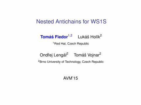
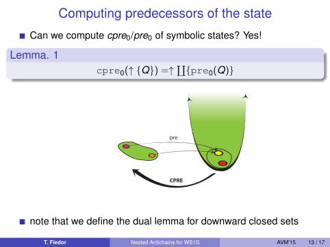
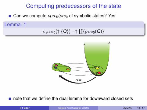
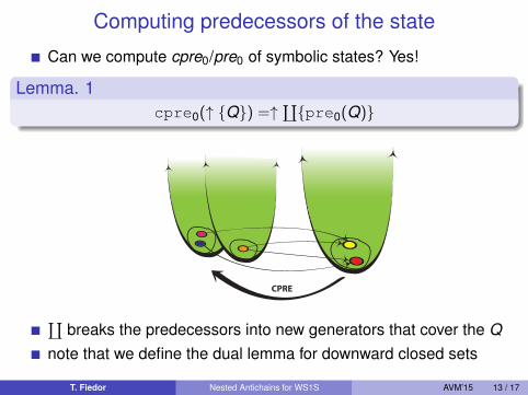
Can we compute cpre0/pre0 of symbolic states?
Yes!
Lemma. 1cpre0(↑ {Q}) =↑
∐{pre0(Q)}
∐breaks the predecessors into new generators that cover the Q
note that we define the dual lemma for downward closed sets
T. Fiedor Nested Antichains for WS1S AVM’15 13 / 17

Computing predecessors of the state
Can we compute cpre0/pre0 of symbolic states? Yes!
Lemma. 1cpre0(↑ {Q}) =↑
∐{pre0(Q)}
∐breaks the predecessors into new generators that cover the Q
note that we define the dual lemma for downward closed sets
T. Fiedor Nested Antichains for WS1S AVM’15 13 / 17
Computing predecessors of the state
Can we compute cpre0/pre0 of symbolic states? Yes!
Lemma. 1cpre0(↑ {Q}) =↑
∐{pre0(Q)}
CPRE
pre
∐breaks the predecessors into new generators that cover the Q
note that we define the dual lemma for downward closed sets
T. Fiedor Nested Antichains for WS1S AVM’15 13 / 17
Computing predecessors of the state
Can we compute cpre0/pre0 of symbolic states? Yes!
Lemma. 1cpre0(↑ {Q}) =↑
∐{pre0(Q)}
CPRE
∐breaks the predecessors into new generators that cover the Q
note that we define the dual lemma for downward closed sets
T. Fiedor Nested Antichains for WS1S AVM’15 13 / 17

Computing predecessors of the state
Can we compute cpre0/pre0 of symbolic states? Yes!
Lemma. 1cpre0(↑ {Q}) =↑
∐{pre0(Q)}
U
CPRE
∐breaks the predecessors into new generators that cover the Q
note that we define the dual lemma for downward closed sets
T. Fiedor Nested Antichains for WS1S AVM’15 13 / 17

Computing predecessors of the state
Can we compute cpre0/pre0 of symbolic states? Yes!
Lemma. 1cpre0(↑ {Q}) =↑
∐{pre0(Q)}
UU U
CPRE
∐breaks the predecessors into new generators that cover the Q
note that we define the dual lemma for downward closed sets
T. Fiedor Nested Antichains for WS1S AVM’15 13 / 17

How to achieve state space reduction
We showed the nested structure of Fm is very complex,
I but we only work with the symbolic representation of the generators(with antichains)
I . . . and the generators of the generators and . . .I this itself is the first source of space reduction
further we prune the generators subsumed by other generatorsI the subsumption relation is computed on nested structure of
symbolic representation of lower levels
T. Fiedor Nested Antichains for WS1S AVM’15 14 / 17

How to achieve state space reduction
We showed the nested structure of Fm is very complex,I but we only work with the symbolic representation of the generators
(with antichains)I . . . and the generators of the generators and . . .I this itself is the first source of space reduction
further we prune the generators subsumed by other generatorsI the subsumption relation is computed on nested structure of
symbolic representation of lower levels
T. Fiedor Nested Antichains for WS1S AVM’15 14 / 17

Experimental results
implemented in dWiNAcompared with MONA:
I on generated and real formulaeI in generic and ∃PNF form
MONA dWiNATime [s] Space [states] Time [s] Space [states]
real normal ∃PNF normal ∃PNF Prefix Prefixlist-reverse-after-loop 0.01 0.01 179 1 326 0.01 100list-reverse-in-loop 0.02 0.47 1 311 70 278 0.02 260bubblesort-else 0.01 0.45 1 285 12 071 0.01 14bubblesort-if-else 0.02 2.17 4 260 116 760 0.23 234bubblesort-if-if 0.12 5.29 8 390 233 372 1.14 28generated3 alternations - 0.57 - 60 924 0.01 504 alternations - 1.79 - 145 765 0.02 585 alternations - 4.98 - 349 314 0.02 706 alternations - TO - TO 0.47 90
T. Fiedor Nested Antichains for WS1S AVM’15 15 / 17

Conclusion and Future Work
Future workI extension to WS2S
• opens whole new world of tree structuresI generalization of symbolic tree representation
• to process logical connectives• to handle general (non-∃PNF) formulae
ConclusionI WS1S = Great expressivity, yet decidable!I Novel approach based on antichainsI Encouraging results in terms of space reduction
T. Fiedor Nested Antichains for WS1S AVM’15 16 / 17

Thank you for your attention!
Any questions?
T. Fiedor Nested Antichains for WS1S AVM’15 17 / 17