Consumer Theory

These notes essentially correspond to chapter 1 of Jehle and Reny.

1 Consumption set

The consumption set, denoted X, is the set of all possible combinations of goods and services that a consumercould consume. Some of these combinations may seem impractical for many consumers, but we allow thepossibility that a consumer could have a combination of 500 Ferraris and 1400 yachts. Assume there is a�xed number of goods, n, and that n is �nite. Consumers may only consume nonnegative amounts of thesegoods, and we let xi 2 R+ be the amount consumed of good i. Note that this implies that the consumptionof any particular good i is in�nitely divisible. The n-vector x consists of an amount of each of the n goodsand is called the consumption bundle. Note that x 2 X and typically X = Rn+. Thus the consumption setis usually the nonnegative n-dimensional space of real numbers.Standard assumptions made about the consumption set are:

1. ? 6= X � Rn+2. X is closed

3. X is convex

4. The n-vector of zeros, 0 2 X.

The feasible set, B (soon we will call it the budget set), is a subset of the consumption set so B � X.The feasible set represents the subset of alternatives which the consumer can possibly consume given his orher current economic situation. Generally consumers will be restricted by the amount of wealth (or incomeor money) which they have at their disposal.

2 Preferences and utility

The basic building block of consumer theory is a binary relation on the consumption set X. The particularbinary relation is the preference relation %, which we call "at least as good as". We can use this preferencerelation to compare any two bundles x1; x2 2 X. If we have x1 % x2 we say "x1 is at least as good as x2".We will make some minimal restrictions about the preference relation %. In general, our goal will be to

make the most minimal assumptions possible. We make two assumptions about our preference relation %:

1. Completeness: For any x1 6= x2 in X, either x1 % x2 or x2 % x1 or both.

2. Transitivity: For any three elements x1, x2, and x3 in X, if x1 % x2 and x2 % x3, then x1 % x3.

Completeness means that the consumer can make choices or rank all the possible bundles in the con-sumption set. Transitivity imposes some minimal sense of consistency on those choices. The book listsa third assumption, re�exivity. However, if the preference relation % is complete and transitive, then wecan also show that it is re�exive. Re�exivity simply means that an element of the consumption set is atleast as good as itself, or x1 % x1 for all x 2 X. These very basic assumptions comprise the conditions ofrationality in economic models. The notion of rationality in economics is one that is often misunderstood �all we assume for a "rational" economic agent is that preferences are complete and transitive (and re�exive).

1

x2

x1A thick indifference set.

x

Whether or not the bulk of society considers a choice to be a good one (say a bright orange tuxedo at aformal event), if an individual agent possesses complete and transitive preferences then that consumer isconsidered to be rational.Now that we have established the preference relation % we can de�ne (1) the strict preference relation

and (2) the indi¤erence relation.

De�nition 1 The strict preference relation, �, on the consumption set X is de�ned as x1 � x2 if and onlyif x1 % x2 but not x2 % x1.

De�nition 2 The indi¤erence relation, �, on the consumption set X is de�ned as x1 � x2 if and only ifx1 % x2 and x2 % x1.

Note that neither � nor � is complete, both are transitive, and only � is re�exive. Once we have � and� we can see that either x1 � x2, x2 � x1, or x1 � x2. Thus, the consumer is able to rank bundles of goods.However, these assumptions of completeness, transitivity, and re�exivity only impose some minimum orderon the ranking of bundles. We will impose a little more structure on our consumer�s preferences.Assumption: Continuity. For all x 2 Rn+, the "at least as good as" set, % (x), and the "no better than

set" - (x) are closed in Rn+.Continuity is primarily a mathematical assumption, but the intuitive reason behind imposing it is so that

sudden preference reversals do not happen.Assumption: Local Nonsatiation. For all x0 2 Rn+, and for all " > 0, there exists some x 2 B"

�x0�\Rn+

such that x � x0.When local nonsatiation is assumed, this means that there is some bundle close to a speci�c bundle which

will be preferred to that speci�c bundle. There is nothing in local nonsatiation that speci�es the directionof the preferred bundle. What local nonsatiation does is rule out "thick" preferences.

2

Assumption: Strict monotonicity. For all x0; x1 2 Rn+, if x0 � x1 then x0 % x1, while if x0 >> x1

then x0 � x1.In a principles or intermediate microeconomics class this is what we would call the "more is better"

assumption. Note that when an individual compares bundles of goods, if the individual has bundle x0 withmore of at least one good (and the same level of all other goods) than is in x1, then this individual deemsx0 at least as good as x1. And if x0 has more of all goods than x1, then the individual strictly prefers x0

to x1.Assumption: Convexity. If x1 % x0, then tx1 + (1� t)x0 % x0 for all t 2 [0; 1].Assumption: Strict convexity. If x1 6= x0 and x1 % x0, then tx1 + (1� t)x0 � x0 for all t 2 (0; 1).Either of these assumptions rules out concave to the origin preferences. The intuition behind these

convexity assumptions is that consumers (generally) prefer balanced consumption bundles to unbalancedconsumption bundles. Thus, since these convex combinations of consumption bundles provide a morebalanced consumption plan, the consumer would prefer them.Alternatively, think about any particular indi¤erence set in R2+. The slope of an indi¤erence curve is

called the marginal rate of substitution.1 If we have strict monotonicity and either form of convexity thenthis means that the marginal rate of substitution should not increase as we move from bundles along thesame indi¤erence which have a lot of good 1 to those which have relatively less of good 1. Thus, when theconsumer has a little of good 1 he should be willing to give up more of good 2 to get an extra unit of good1 than when he has a lot of good 1.As a summary, the assumptions of completeness, transitivity, and re�exivity are the basis for the rational

consumer. The assumption of continuity is primarily a mathematical one to make the problem slightly moretractable. The remaining assumptions represent assumptions about a consumer�s tastes.

2.1 Utility

The utility function is a nice way to summarize preferences, particularly if one wants to use calculus methodsto solve problems (as we will want to do). We can establish results that show that with a minimal amountof structure that there will be a utility function which represents our preference relation %.

De�nition 3 A real-valued function u : Rn+ ! R is called a utility function representing preference relation%, if for all x0; x1 2 Rn+, u

�x0�� u

�x1�() x0 % x1.

The question is which assumptions that we made about our preference relation will be needed to establishthat a utility function which represents % exists? There is a theorem which states that all we need iscompleteness, transitivity, re�exivity, and continuity. Note that monotonicity, convexity (of any type), andlocal nonsatiation are NOT needed to guarantee the existence of a utility function which represents %.

Theorem 4 If the binary relation % is copmlete, re�exive, transitive, and continuous then there exists acontinuous real-valued function, u : Rn+ ! R, which represents %.

We will not go through the proof of this theorem but we will use the result. Note that in the book theprovide the proof of a slightly less general result in Theorem 3.1 as they assume strict monotonicity. Again,note that strict monotonicty is NOT required to ensure the existence of a utility function which represents%.When specifying utility functions economists are primarily concerned with preserving ordinal relation-

ships, not cardinal ones. Thus, two utility functions which preserve the order of preferences over bundles willbe viewed the same UNLESS the cardinality of the utility function is important for a particular application.So if there are two utility functions, u (x1; x2) = x1 + x2 and v (x1; x2) = x1 + x2 + 5 it should be clear thatthe resulting utility level from the same (x1; x2) bundle is higher in v (�) than in u (�). However, since theorder of preferences over bundles is preserved between the two utility functions, they are generally viewedthe same by economists.Now consider the same function u (x1; x2) = x1 + x2 and another function g (x1; x2) = x1x2. If we look

at the table for three di¤erent bundles of x1 and x2 we see that:1Note that this text refers to the marginal rate of substitution as a positive number even though the slope will be nonpositive

for convex preferences.

3

x1 x2 u (x1; x2) g (x1; x2)8 0 8 02 2 4 4Since u (8; 0) > u (2; 2) but g (2; 2) > g (8; 0), we can see that these utility functions do not preserve the

order of preferences for the bundles so that they are not viewed as the same by economists. Given this notionof ordinality of utility functions, we have the following theorem.

Theorem 5 Let % be a preference relation on Rn+ and suppose u (x) is a utility function that representsit. Then v (x) also represents % if and only if v (x) = f (u (x)) for every x, where f : R ! R is strictlyincreasing on the set of values taken on by u.

We have been developing a model of the consumer based upon the preference relation % and someassumptions (hopefully realistic) about the preference relation. We would like to represent our preferencerelation % with a utility function (so that we can use calculus to solve the problem). Based on a rationalpreference relation %, we ensure that the utility function has certain properties when we impose monotonicityand convexity on our preference relation %.

Theorem 6 Let % be represented by u : Rn+ ! R. Then:

1. u (x) is strictly increasing if and only if % is strictly monotonic

2. u (x) is quasiconcave if and only if % is convex

3. u (x) is strictly quasiconcave if and only if % is strictly convex

In order to facilitate �nding a solution to the consumer�s problem we impose di¤erentiability of theconsumer�s utility function u (�). Like continuity, di¤erentiability is a mathematical assumption. Whenu (�) is di¤erentiable, we can �nd the �rst-order partial derivatives. The �rst-order partial derivative ofu (x) with respect to xi,

@u(x)@xi

, is called the marginal utility of good i. We can now de�ne the marginal rateof substitution (MRS) between two goods as the ratio of the marginal utilities of the two goods. So themarginal rate of substitution of good i for good j is:

MRSij (x) �@u (x) =@xi@u (x) =@xj

(1)

What theMRS tells us is the rate at which we can substitute one good for the other, keeping utility constant.

3 Consumer�s problem

The consumer�s general problem is to choose x� 2 X such that x� % x for all x 2 X. However, whenX = Rn+ this simply means that the consumer chooses an in�nite amount of all goods. Thus, we restrictthe consumption set to a feasible set B � X = Rn+. The consumer�s problem then is to choose x� 2 B suchthat x� % x for all x 2 B. Since it is easier to work with utility functions than preference relations, we makethe following assumptions about our preference relation %. Assume the preference relation % is complete,re�exive, transitive, continuous, strictly monotonic, and strictly convex on Rn+. This means that % can berepresented by a real-valued utility function that is continuous, strictly increasing, and strictly quasiconcaveon Rn+.

3.1 Market economy

In a market economy the consumer will face a price vector p, where there is one price for each of the n goods.We assume that the price vector p is strictly positive, or p >> 0 so that each pi > 0. Also, the price vectoris �xed and exogenous to the consumer�s decisions �therefore, an individual consumer has no impact on theprice of ANY good.2 The consumer also has a �xed amount of money y > 0. This is an endowment (for

2This is just an assumption that can be changed.

4

B

x2

x1

y/p2

y/p1

now), meaning that the consumer simply receives this sum of money y. The consumer CANNOT spendmore than this particular amount of income. The combination of positive prices, �nite income, and theassumption that the consumer cannot spend more than his income restrict the consumption set, X, to thefeasible set B. Thus, the consumer�s budget constraint is given by:

nXi=1

pixi � y (2)

With the budget constraint we can now create the budget set B, where:

B =�xjx 2 Rn+; px � y

(3)

When there are 2 goods, the budget set B is:Because of our assumptions about % and its relationship to u (�), we can formulate the consumer�s problem

as:maxx2Rn+

u (x) subject to px � y (4)

Thus, our consumer�s problem is an inequality constrained maximization problem. The solution to theproblem, x�, is the x such that u (x�) � u (x) for all x 2 B. Given the relationship between % and u (�),this means that x� % x for all x 2 B and that x� solves our original consumer�s problem with the preferencerelation. Note that the particular solution x� will depend upon the parameters of the problem, or theprices and income that the consumer faces. Thus we will write x� as x (p; y), with xi (p; y) representing theparticular quantity of good i.A few general results. We "know" that the optimal bundle x� (p; y) will lie on the budget constraint,

or where px = y. This is because preferences are strictly monotonic. If the consumer chooses a bundle ofgoods on the interior of the budget set (not along the budget constraint), then that consumer will alwaysbe able to �nd another bundle that is preferred to the chosen bundle (because there is some feasible bundlewith more of both goods). Also, because y > 0 and x� 6= 0, we know that the consumer consumes a positiveamount of at least one good. Since % is assumed to be strictly convex, the solution x� (p; y) will be unique,

5

so that x� (p; y) is a demand function that speci�es the amount of each good a consumer will choose givenprice vector p and income level y. We call these x (p; y) the Marshallian demand functions. To �nd them,simply solve the inequality constrained maximization problem by setting up the Lagrangian, di¤erentiating,and solving for each of the xi.

L (x; �) = u (x) + � [y � px] (5)

Assuming that x� >> 0, we know there is a �� � 0 such that (x�; ��) satisfy:

@L@xi

=@u (x)

@xi� �pi = 0 i = 1; :::; n (6)

y � px� � 0 (7)

�� [y � px�] = 0 (8)

Since we are assuming % is strictly monotone we have y� px� = 0, which leaves us with n+1 equations andn + 1 unknown. While it�s possible that ru (x�) = 0 it is unlikely that this is so we assume ru (x�) 6= 0.So we will have @u(x�)

@xi> 0 for at least one i = 1; :::; n. Since pi > 0, we have that �

� > 0 because from:

@u (x�)

@xi= ��pi (9)

@u (x�)

@xi=pi = �� > 0 (10)

For any two goods we can rewrite this as:

@u (x�)

@xi=pi =

@u (x�)

@xj=pj (11)

@u(x�)@xi

@u(x�)@xj

=pipj

(12)

Recall that @u(x�)

@xi=@u(x

�)@xj

is the marginal rate of substitution between goods i and j. Thus, at the optimum,the MRS between goods i and j will be equal to the slope of the budget constraint. This is simply themathematical result that one would see in an intermediate microeconomics class. The �gure illustrates thatthe consumer optimum is where the indi¤erence curve is tangent to the budget constraint (point E), whilealso showing why other points cannot be optimal. If the consumer were at point G, there are many bundlesthat are strictly preferred to G (including point E). While point F is on the budget constraint it is notoptimal as it is indi¤erent to point G (since it lies on the same indi¤erence curve) and we have already seenthat G is not optimal.

3.1.1 Example

Consider the utility function u (x1; x2) = x�1 x�2 . The prices of good 1 is p1 > 0 and the price of good 2 is

p2 > 0. The consumer has income y > 0. The consumer�s problem is:

maxx1�0;x2�0

x�1 x�2 s.t. p1x1 + p2x2 � y (13)

We can form the Lagrangian, di¤erentiate with respect to x1, x2, and �, and �nd the solution as:

L (x1; x2; �) = x�1x�2 + � [y � p1x1 � p2x2] (14)

Di¤erentiating we have:

@L@x1

= �x��11 x�2 � �p1 = 0 (15)

@L@x2

= �x�1x��12 � �p1 = 0 (16)

y � p1x1 � p2x2 � 0 (17)

� [y � p1x1 � p2x2] = 0 (18)

6

Good B

I2

I1

E

F

G

7

Again, the budget constraint will hold with equality so:

�x��11 x�2 � �p1 = 0�x�1 x

��12 � �p1 = 0

y � p1x1 � p2x2 = 0(19)

Simplifying we have:�x��11 x�2

p1=

�x�1 x��12

p2x�2x��12

=�x�1 p1

�x��11 p2

x2 =x1p1��p2

(20)

Now, substituting into the budget constraint we have:

y � p1x1 � p2�x1p1��p2

�= 0

y � p1x1 � ��p1x1 = 0

p1x1 +��p1x1 = y

x1

�p1 +

��p1

�= y

x1

��+�� p1

�= y

x1 =�y

(�+�)p1

(21)

To �nd x2 we simply plug x1 back into x2 =x1p1��p2

:

x2 =x1p1��p2

x2 =�y

(�+�)p1

p1��p2

x2 =�y

(�+�)p2

(22)

Thus, if we have done the calculus and algebra correctly, we have:

x�1 (p; y) =�y

(�+ �) p1(23)

x�2 (p; y) =�y

(�+ �) p2(24)

We can check that at the optimum we have:

MRS = pipj

orMU1p1

= MU2p2

(25)

Recall that u (x1; x2) = x�1 x�2 , so that:

MU1 = �x��11 x�2 (26)

MU2 = �x�1x��12 (27)

Substituting x�1 and x�2 and dividing by the respective prices we have:

MU1p1

=MU2p2

(28)

�x��11 x�2p1

=�x�1 x

��12

p2(29)

�x2p1

=�x1p2

(30)

� �y(�+�)p2

p1=

� �y(�+�)p1

p2(31)

��y

(�+ �) p2p1=

��y

(�+ �) p1p2(32)

8

Technically we should check to make sure that the interior solution IS the optimal solution, and that thereis not a better solution at a corner (when either x�1 = 0 and x�2 =

yp2or x�1 =

yp1and x�2 = 0). However,

in this problem u (x1; x2) = x�1x

�2 , so if either x1 or x2 equals 0 then the utility function is unde�ned. So

the consumer should buy at least some small positive amount of each good with this utility function. Using� = 1

2 , � =12 , p1 = 5, p2 = 10, and y = 150, the following picture is a two-dimensional representation of the

consumer�s problem:

0 2 4 6 8 10 12 14 16 18 20 22 24 26 28 30 32 340

5

10

15

20

x1

x2

3.1.2 Second example

Now suppose that u (x1; x2) = �x1 + �x2, with prices p1 > 0 and p2 > 0 respectively, and y > 0. We canstart by setting up the Lagrangian and following our steps:

L (x1; x2; �) = �x1 + �x2 + � [y � p1x1 � p2x2] (33)

Di¤erentiating we have:

@L@x1

= �� �p1 = 0 (34)

@L@x2

= � � �p2 = 0 (35)

y � p1x1 � p2x2 � 0 (36)

� [y � p1x1 � p2x2] = 0 (37)

While the budget constraint will still hold with equality, combining the �rst two equations we get:

�

p1=�

p2= � (38)

Since this condition does not depend on x1 or x2 it will only be true for certain parameters. If theparameters are such that �

p1= �

p2, then any combination of x1 and x2 such that the budget constraint holds

with equality will be a solution to the problem (in this case we have a Marshallian demand correspondence,not a Marshallian demand function). However, if �

p16= �

p2, then the consumer would like to spend all of his

income on either x1 or x2. Thus we can check the "corners" to see which gives higher utility. The nextsection discusses checking corner solutions more generally.

9

3.1.3 A more general example

While we may not have a guarantee of an interior solution, we still want to restrict x1 � 0 and x2 � 0. So,our consumer�s problem is still to maximize utility subject to his budget constraint, but now we have theadditional constraints that x1 � 0 and x2 � 0. Writing this out for a two good problem we have:

maxx1;x2

u (x1; x2) s.t. p1x1 + p2x2 � y, x1 � 0, x2 � 0.

We have already seen this general example for an inequality constrained optimization problem. For ourspeci�c problem, we need all of the inequality constraints as � constraints. Since x1 � 0 and x2 � 0 arealready written in this manner, that just leaves rewriting the budget constraint as y�p1x1�p2x2 � 0. Nowwe can form the Lagrangian:

L (x1; x2; �1; �2; �3) = u (x1; x2) + �1 [y � p1x1 � p2x2] + �2 [x1] + �3 [x2]

We will now have a full set of Kuhn-Tucker conditions for both our choice variables and our Lagrangemultipliers:

@L@x1

= @u@x1

� �1p1 + �2 � 0; x1 � 0; x1 � @L@x1

= 0@L@x2

= @u@x2

� �1p2 + �3 � 0; x2 � 0; x2 � @L@x2

= 0@L@�1

= y � p1x1 � p2x2 � 0; �1 � 0; �1 � y � p1x1 � p2x2 = 0@L@�2

= x1 � 0; �2 � 0; �2 � x1 = 0@L@�3

= x2 � 0; �3 � 0; �3 � x2 = 0

:

Note that in this case we have complementary slackness conditions for the choice variables because we areuncertain as to whether or not the constraints are binding. Technically we would have 32 cases to check,one for each possible combination of x1, x2, �1, �2, and �3 being either strictly positive or zero. However,we know that the budget constraint will bind, and we know that either x1 � 0 or x2 � 0 so we really onlyhave to check if x1 = 0 or x2 = 0 (with more goods, for example three goods, we would still have to checkwhether x1 = x2 = 0 and x3 > 0, x1 = x3 = 0 and x2 > 0, or x2 = x3 = 0 and x1 > 0).In general, the process I would use to �nd the optimal value would be to set up the Lagrangian function

and assume an interior solution (or argue that the solution must be interior) and then check the potentialcorner solutions. If you cannot �nd a unique optimal interior solution (which would be the case if withour linear utility function example we had �

p1= �

p2), then I would suggest checking the various "corners".

Continuing with the linear function example, if u�yp1; 0�> u

�0; yp2

�, then the consumer would choose to

consume only x1. This would be true if:�y

p1>�y

p2(39)

To make it easier to see that this is optimal, assume � = �. Then the consumer would simply choose toconsume only the good that is less expensive.

4 Additional formulations of the consumer�s problem

We will look at two additional formulations of the consumer�s problem. In the �rst we create the consumer�sindirect utility function. The indirect utility function possesses a few useful properties that we can takeadvantage of. In the second we formulate the consumer�s problem as an expenditure minimization problem.In this problem, the consumer�s goal is to set a target level of utility and then �nd the bundle that minimizesexpenditure.

4.1 Indirect utility function

When we set up the consumer�s utility function we have the consumer maximizing u (x) by choosing a bundleof goods. For any set of prices p and income y the consumer chooses x (p; y) that maximizes u (x). Thevalue of the utility function at x (p; y) is the maximum utility for a consumer given prices p and income y.

10

We can de�ne a function that relates the maximum value of utility to the di¤erent price vectors and incomelevels a consumer may face. De�ne a real-valued function v : Rn+1++ ! R as:

v (p; y) = maxx2Rn+

u (x) s.t. px � y (40)

The function v (p; y) is called the indirect utility function because the consumer is not directly maximizing vbut indirectly maximizing v by maximizing u. If u (x) is continuous and strictly quasiconcave, then there isa unique solution to this optimization problem, and that is the consumer�s demand function x (p; y). Thereis a relationship between v (p; y) and u (x):

v (p; y) = u (x (p; y))

for some price vector p and income level y. There are a number of properties the indirect utility functionpossesses and they are summarized in the theorem below:

Theorem 7 If u (x) is continuous and strictly increasing on Rn+, then v (p; y) is:

1. Continuous on Rn++ � R+

2. Homogeneous of degree zero in (p; y)

3. Strictly increasing in y

4. Decreasing in p

5. Quasiconvex in (p; y)

6. Roy�s Identity: If v (p; y) is di¤erentiable at�p0; y0

�and @v

�p0; y0

�=@y 6= 0, then:

xi�p0; y0

�= �

@v�p0; y0

�=@pi

@v (p0; y0) =@y; i = 1; :::; n

The �rst �ve points are simply restrictions on v (p; y) given restrictions on u (x). The sixth point greatlysimpli�es �nding the consumer�s Marshallian demand function if the indirect utility function is known.While we will not prove these results (proofs and sketches of proofs are in the text), we will work throughan example using the following indirect utility function:

v (p; y) =��11 �

�22 �

�33 y

p�11 p�22 p

�33

with �i > 0 and �1 + �2 + �3 = 1.This indirect utility function can be found by solving the consumer�s maximization problem and substi-

tuting the Marshallian demands into the utility function. Consider:

u (x1; x2; x3) = x�11 x

�22 x

�33 (41)

where �i > 0 and �1 + �2 + �3 = 1. We know that:

xi (p; y) =�iy

pi(42)

so that:

v (p; y) =

��1y

p1

��1 ��2yp2

��2 ��3yp3

��3(43)

v (p; y) =��11 �

�22 �

�33 y

�1+�2+�3

p�11 p�22 p

�33

(44)

v (p; y) =��11 �

�22 �

�33 y

p�11 p�22 p

�33

(45)

11

To show that v (p; y) is homogeneous of degree zero, we have:

v (tp; ty) =��11 �

�22 �

�33 ty

(tp1)�1 (tp2)

�2 (tp3)�3

v (tp; ty) =��11 �

�22 �

�33 ty

t�1+�2+�3p�11 p�22 p

�33

v (tp; ty) =��11 �

�22 �

�33 y

p�11 p�22 p

�33

v (tp; ty) = v (p; y)

To show that v (p; y) is increasing in y we simply �nd the partial derivative with respect to y and show thatthis derivative is strictly positive:

@v (p; y)

@y=��11 �

�22 �

�33

p�11 p�22 p

�33

> 0

This partial derivative is strictly greater than 0 since pi > 0 and �i > 0.To show that v (p; y) is decreasing in p, we can �nd the partial derivative with respect to any price we

rewrite as:

v (p; y) =y��ii �

�jj �

�kk p

��ii

p�jj p

�kk

@v (p; y)

@pi=

��i��ii ��jj �

�kk yp

��i�1i

p�jj p

�kk

@v (p; y)

@pi=

��i��ii ��jj �

�kk y

p�i+1i p�jj p

�kk

< 0

To provide an example of Roy�s identity we have:

@v (p; y)

@pi=

��i��ii ��jj �

�kk y

p�i+1i p�jj p

�kk

@v (p; y)

@y=

��ii ��jj �

�kk

p�ii p�jj p

�kk

Taking the ratio:

xi (p; y) = �

��i��ii �

�jj �

�kk y

p�i+1

i p�jj p

�kk

��ii �

�jj �

�kk

p�ii p

�jj p

�kk

xi (p; y) =�iy

p�i+1i p�jj p

�kk

� p�ii p�jj p

�kk

xi (p; y) =�iy

pi

Note that these demand functions are similar to those that we found when working through the standardmaximization problem when u (x1; x2) = x�1 x

�2 . Recall that the demand functions in that example were

x1 (p; y) =�y

(�+�)p1and x2 (p; y) =

�y(�+�)p2

. If we impose �+ � = 1 (as we have done in the indirect utilityfunction example), we have the same form for the demand functions. So the indirect utility function for the

Cobb-Douglas utility function (with 3 goods) is v (p; y) =��ii �

�jj �

�kk y

p�11 p

�22 p

�33

.

4.2 Expenditure function

With the standard utility maximization problem we assume that the consumer has a �xed budget constraintand then determines what the maximum level of utility can be achieved given p and y. However, we can

12

formulate a similar problem where the consumer �xes a target level of utility and then chooses the incomelevel which minimizes expenditure to attain that target level of utility. In essence, the indi¤erence curveis �xed and the consumer is shifting the budget constraint back and forth trying to �nd the lowest possiblecost to achieve his target utility level.Formally we can de�ne the expenditure function as:

e (p; u) = minx2Rn+

px subject to u (x) � u (46)

The solution to the expenditure minimization problem is known as the Hicksian demand function, of xh (p; u).If we �nd xh (p; u), then we know that e (p; u) = p � xh (p; u) because this is the bundle which minimizesexpenditure for utility level u and prices p. What these demand functions tell us is how purchases changewhen we hold utility constant and there is a price change of one good. Let�s use u (x) = x�11 x

�22 x

�33 with

�1 + �2 + �3 = 1 to �nd the Hicksian demands.Set up the Lagrangian:

L (x1; x2; x3; �) = p1x1 + p2x2 + p3x3 + � [u� x�11 x�22 x

�33 ] (47)

Di¤erentiating:

@L@x1

= p1 � ��1x�1�11 x�22 x�33 = 0 (48)

@L@x2

= p2 � ��2x�2�12 x�11 x�33 = 0 (49)

@L@x3

= p3 � ��3x�3�13 x�22 x�11 = 0 (50)

@L@�

= u� x�11 x�22 x

�33 = 0 (51)

We �nd that:

p1

�1x�1�11 x�22 x

�33

=p2

�2x�2�12 x�11 x

�33

(52)

�2x1p2

=�1x2p1

(53)

x1 =�1x2p2p1�2

(54)

We also have:

p3

�3x�3�13 x�22 x

�11

=p2

�2x�2�12 x�11 x

�33

(55)

�2x3p2

=�3x2p3

(56)

x3 =�3x2p2p3�2

(57)

13

Plugging into the utility constraint we have:

u���1x2p2p1�2

��1x�22

��3x2p2p3�2

��3= 0 (58)�

�1x2p2p1�2

��1x�22

��3x2p2p3�2

��3= u (59)

x�1+�2+�32

��1p2p1�2

��1 ��3p2p3�2

��3= u (60)

u

�p1�2�1p2

��1 �p3�2�3p2

��3= x2 (61)

up�11 �

�12 p

�33 �

�32

��11 p�12 �

�33 p

�32

= x2 (62)

up�11 p

�33 �

�1+�32

p�1+�32 ��11 ��33

= x2 (63)

up�11 p

�33 �

�1+�32

p1��22 ��11 ��33

� ��22

��22= x2 (64)

up�11 p

�33 �

�1+�2+�32

p1��22 ��11 ��33 �

�22

= x2 (65)

up�11 p

�33 �2p

�2�12

��11 ��33 �

�22

= x2 (66)

To clarify, we are �nding the Hicksian demands when solving the expenditure minimization problem, so

xh2 (p; u) = up�11 p

�33 �2p

�2�12

��11 ��33 �

�22

(67)

We can then �nd that:

xh1 (p; u) = up�22 p

�33 �1p

�1�11

��11 ��33 �

�22

(68)

xh3 (p; u) = up�11 p

�22 �3p

�3�13

��11 ��33 �

�22

(69)

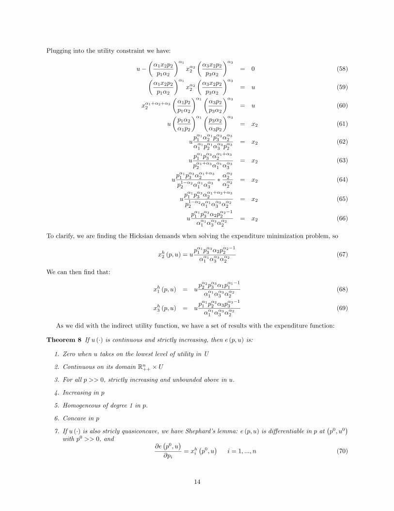
As we did with the indirect utility function, we have a set of results with the expenditure function:

Theorem 8 If u (�) is continuous and strictly increasing, then e (p; u) is:

1. Zero when u takes on the lowest level of utility in U

2. Continuous on its domain Rn++ � U

3. For all p >> 0, strictly increasing and unbounded above in u.

4. Increasing in p

5. Homogeneous of degree 1 in p.

6. Concave in p

7. If u (�) is also stricly quasiconcave, we have Shephard�s lemma: e (p; u) is di¤erentiable in p at�p0; u0

�with p0 >> 0, and

@e�p0; u

�@pi

= xhi�p0; u

�i = 1; :::; n (70)

14

Again, we will take these without proof although the text has proofs. Expenditure is zero when utilityis at its lowest possible level �there is no need to spend any money to achieve that level. As u increases,expenditure must increase (holding prices constant). Also, expenditure is unbounded as utility increases.If prices (or one price) increase, then expenditure does not decrease. There are also homogeneity, concavity,and continuity results. Finally, we can derive the Hicksian demand functions directly from the expenditurefunction. Recall that the expenditure function is essentially px, or p1x1 + p2x2 + :::+ pnxn. Thus we cansimply di¤erentiate the expenditure function to �nd the Hicksian demands. As an example, consider thefollowing expenditure function:

e (p; u) =up�11 p

�22 p

�33

��11 ��22 �

�33

(71)

where �1 + �2 + �3 = 1. The expenditure function is zero when u = 0 (from a Cobb-Douglas this is thelowest level of utility we can have). It is strictly increasing in u and unbounded above in u. It is increasingin any price. For homogeneity of degree 1 in prices we have:

e (tp; u) =u (tp1)

�1 (tp2)�2 (tp3)

�3

��11 ��22 �

�33

(72)

e (tp; u) =ut�1p�11 t

�2p�22 t�3p�33

��11 ��22 �

�33

(73)

e (tp; u) =t�1+�2+�3up�11 p

�22 p

�33

��11 ��22 �

�33

(74)

e (tp; u) = te (p; u) (75)

For Shephard�s lemma, we have:

@e (p; u)

@pi=u�ip

�i�1i p

�jj p

�kk

��ii ��jj �

�kk

= xhi (p; u) (76)

4.2.1 Relating v (p; y) and e (p; u)

There is a relationship between v (p; y) and e (p; u). If we �x p and y and let u = v (p; y). As per thede�nition of v (p; y), u is the maximum utility that can be attained when prices are p and income is y. Also,if the consumer wishes to achieve utility level u at prices p, then the consumer will be able to achieve thatlevel of utility with expenditure y. But the expenditure minimization function tells us the LEAST amountof expenditure needed to achieve utility level u at prices p. Thus, we would need:

e (p; u) � y (77)

e (p; v (p; y)) � y (78)

We can perform a similar analysis if we �x p and u. We know that at prices p and utility u, we will need:

v (p; y) � u (79)

v (p; e (p; u)) � u (80)

Now we have a theorem explaining the relationship between e (p; u) and v (p; y).

Theorem 9 Let v (p; y) and e (p; u) be the indirect utility function and expenditure function for some con-sumer whose utility function is strictly increasing and continuous. Then for all p >> 0, y � 0, and u 2 U :

1. e (p; v (p; y)) = y

2. v (p; e (p; u)) = u

15

Again, we forgo the proof and use an example. We will use

v (p; y) =��11 �

�22 �

�33 y

p�11 p�22 p

�33

(81)

e (p; u) =up�11 p

�22 p

�33

��11 ��22 �

�33

(82)

So:

e (p; v (p; y)) =

���11 �

�22 �

�33 y

p�11 p

�22 p

�33

�p�11 p

�22 p

�33

��11 ��22 �

�33

(83)

e (p; v (p; y)) = y (84)

Also:

v (p; e (p; u)) =��11 �

�22 �

�33

�up

�11 p

�22 p

�33

��11 �

�22 �

�33

�p�11 p

�22 p

�33

(85)

v (p; e (p; u)) = u (86)

Theorem 10 Given that u (�) is strictly increasing, continuous, and strictly quasiconcave, the followingrelations hold between the Marshallian and Hicksian demand functions when p >> 0, y � 0, and u 2 U .

1. xi (p; y) = xhi (p; v (p; y))

2. xhi (p; u) = xi (p; e (p; u))

This �rst relationship states that the Marshallian demand for prices p and income y are identical to theHicksian demand at prices p when utility is v (p; y). Alternatively, the Hicksian demands at p and u areequal to the Marshallian demands when prices are p and expenditure is given by y = e (p; u).As an example:

xhi (p; u) =u�ip

�i�1i p

�jj p

�kk

��ii ��jj �

�kk

(87)

xhi (p; v (p; y)) =

�y�

�ii �

�jj �

�kk

p�ii p

�jj p

�kk

��ip

�i�1i p

�jj p

�kk

��ii ��jj �

�kk

(88)

xhi (p; v (p; y)) =�iyp

�i�1i

p�ii(89)

xhi (p; v (p; y)) =�iy

pi(90)

xhi (p; v (p; y)) = xi (p; y) (91)

Also:

xi (p; y) =�iy

pi(92)

xi (p; e (p; u)) =

�i

�up

�ii p

�jj p

�kk

��ii �

�jj �

�kk

�pi

(93)

xi (p; e (p; u)) =u�ip

�i�1i p

�jj p

�kk

��ii ��jj �

�kk

(94)

xi (p; e (p; u)) = xhi (p; u) (95)

16

5 Properties of consumer demand

In principles and intermediate microeconomics you typically study demand functions �rst and then (perhaps)utility or consumer theory. Here we have started with the utility function and used the utility functionto derive demand functions. Right now we are concerned with individual demand functions. When youstudied them at the undergraduate level, we simply stated things like "The Law of Demand states thatthere is an inverse relationship between the price of a good and its quantity demanded". You were usuallyasked to take that on faith, and intuitively it makes sense �holding everything else constant, if you raisethe price of a good its quantity demanded should fall. Now, we will see that the demand functions usedin the undergraduate classes were a direct result of the assumptions that we have been making about ourpreference relation %, our utility function u (�), and our feasible set.Two of the most basic concepts are relative prices and real income. Economists are more concerned

with relative prices rather than actual prices, as consumers care about the quantity of money only in termsof the amount of goods and services a particular amount of money can buy (people have little utility forthe actual good "money", other than that it serves as a medium of exchange by which they can purchasegoods). Thus, we can discuss prices in terms of relative prices �namely, we can �x the price of one good(call it the numeraire) and then denominate all other goods in that numeraire. Economists also discusspurchasing power in terms of real income. If one individual has $10,000 and the other has $100,000 thenwe tend to think that the person with $100,000 is better o¤ than the one with $10,000. This is true ifprices are the same, but if the individual with $10,000 faces a price vector that is 1

100

thof the price vector

that the individual with $100,000 (so that the person with $100,000 faces prices that are 100x higher), thenthe person with $10,000 will be better o¤ than the person with $100,000 because the person with $10,000can purchase more goods. If consumer preferences are complete, transitive, re�exive, strictly monotonic,and strictly convex, then Marshallian demand functions are homogeneous of degree zero (which essentiallymeans that if you increase all prices and wealth by the same proportion the consumer�s Marshallian demanddoes not change) and budget balancedness holds (the budget constraint holds with equality).

5.1 Income and substitution e¤ects

While �nding the solution to the UMP or the EMP is an important step, many economists focus on whathappens when something changes in the economic system. We will begin by discussing price changes in Hick-sian demand, as Hicksian demand satis�es the law of demand (price increases, quantity demanded decreases)while Walrasian demand may or may not. However, Hicksian demand is a function of an unobservable vari-able, utility. Walrasian demand, however, is a function of the observable variables (or at least variables thatwe might be able to observe) price and wealth (or income).We have that the own-price derivatives of Hicksian demand are nonpositive because Hicksian demand

follows the compensated law of demand. This means

@xhi (p; u)

@pi� 0:

Recall that with a Hicksian demand change we are determining how much quantity demanded falls whenprice increases by keeping the consumer on the same indi¤erence curve (or at the same utility level).Giventhat our indi¤erence curves are downward sloping, it is necessarily the case that Hicksian demand decreases(if we have a di¤erentiable utility function and are at an interior solution) as the �gure above shows orremains at zero (if we have a utility function that is nondi¤erentiable and are at an interior solution �westay at the same point, think of perfect complements �or if we are at a corner solution). We can also showthis mathematically as we have:

@e (p; u)

@pi= xhi (p; u)

@2e (p; u)

@pi@pi=

@xhi (p; u)

@pi� 0

This is because the expenditure function is a concave function.

17

Good B

Good A

xA1

xB1

xA2

xB2

18

Now consider the cross-price derivative of Hicksian demand xhi (p; u) with respect to the price of good k,

pk. If @xhi (p;u)@pk

� 0 then goods i and k are complements or complementary goods, because as the price ofgood k increases the Hicksian demand for good i decreases. Thus we are consuming less of good k and less

of good i when pk increases. If@xhi (p;u)@pk

� 0 then goods i and k are substitutes because as the price of goodk increases the Hicksian demand for good i increases. Note that if the cross-price derivative is equal to zerothen the goods could be classi�ed as either substitutes or complements. However, consider what it meansif the cross-price derivative truly is zero �a change in pk has no e¤ect on the Hicksian demand for goodi. Thus the two goods could be classi�ed as independent. We know that there must be at least one goodwhich which has a nonpositive substitution e¤ect for any speci�c good in the economy. To see this, considerthe 2-good case. If the price of good k increases, then the consumption of good k will decrease (unless theconsumer is at a corner solution) because Hicksian demand follows the compensated law of demand. Now,if the consumer is to remain at the same utility level, and he is consuming less of good k, then he mustconsume more of good i.

5.1.1 Decomposing Hicksian demand changes

The purpose of using Hicksian demand is because Hicksian demand follows the compensated law of demand.But, we cannot observe Hicksian demand because one of its arguments is unobservable (utility level). Wecan exploit the relationship between Hicksian demand and Walrasian demand to obtain information on pricee¤ects.3

Proposition 11 (The Slutsky Equation) Suppose that u (�) is a continuous utility function representinglocally nonsatiated preference relation % de�ned on X = RN+ . Then for all (p; y) and u = v (p; y) we have

@xhi (p; u)

@pk=@xi (p; y)

@pk+@xi (p; y)

@yxk (p; y) for all i; k.

Or, rewriting in terms of the cross-price e¤ect of the Walrasian demand:

@xi (p; y)

@pk=@xhi (p; u)

@pk+@xi (p; y)

@yxk (p; y) for all i; k.

Proof. We know that xhi (p; u) = xi (p; e (p; u)) at the optimal solution to the consumer�s problem. We candi¤erentiate with respect to pk and evaluate at p and u.

Statement Reason

1. @xhi (p;u)@pk

= @xi(p;e(p;u))@pk

+ @xi(p;e(p;u))@y

@e(p;u)@pk

1. Chain rule for di¤erentiation

2. @xhi (p;u)@pk

= @xi(p;e(p;u))@pk

+ @xi(p;e(p;u))@y xhk (p; u) 2. Earlier result on relation

of e (p; u) to xh (p; u)3. xhk (p; u) = xk (p; e (p; u)) = xk (p; y) 3. Earlier result on relation

of xhk (p; u) to xk (p; y)4. e (p; u) = y 4. Earlier result on relation

of e (p; u) to y

5. @xhi (p;u)@pk

= @xi(p;y)@pk

+ @xi(p;y)@y xk (p; y) 5. Substitution

For the Walrasian demand, the change in quantity of good i with respect to a change in the price ofgood k is known as the Total E¤ect of the change in price of good k. The total e¤ect is decomposed into

the Substitution E¤ect�@xhi (p;u)@pk

�and the Income (or Wealth) E¤ect

�@xi(p;y)@y xk (p; y)

�. The Substitution

E¤ect is the change in quantity demanded of good i due to the fact that good i is now relatively more (less)expensive if the price of another good (say good k) increases (decreases) when the prices of all other goodsstay the same. Thus, if the price of a good k increases, we would expect that a consumer would purchasemore of a second good i because i is now a relatively less expensive substitute (unless of course the goodsare complements). The Income E¤ect is the change in quantity demanded of good i due to the fact that

3For a recent reference on using the Slutsky equation in empirical work, see Fisher, Shively, and Buccola (2005). ActivityChoice, Labor Allocation, and Forest Use in Malawi. Land Economics, Vol. 81:4

19

x1

x2

Budget constraint when p1 increases

Initial budget constraint

Hicksian compensation budget constraint

TE (+)SE (­)

IE (­)

x1

x2

xh

Figure 1: Decomposing the e¤ect of a price change on a Gi¤en good.

the consumer has control over how he spends his wealth. There need be no actual change in y for there tobe an income e¤ect, but if the price of good k increases, then the consumer may not just decide to reduceconsumption of good k at the rate of the price increase. For example, if pk doubles, the consumer may keepconsumption of good i the same and simply reduce consumption of good k to 1

2 its previous level, but is notrequired to act in this manner. The consumer may cut consumption by more (or less) than 1

2 and adjustconsumption of good i accordingly. The consumer may even increase the amount of good k when a priceincrease occurs �this is the case of a Gi¤en good, and it occurs because the Income E¤ect overwhelms theSubstitution E¤ect. Consider the Slutsky equation for a change in the own-price of a good:

@xi (p; y)

@pi=@xhi (p; u)

@pi+@xi (p; y)

@yxi (p; y)

We know that if pi increases that the Substitution E¤ect�@xhi (p;u)@pi

�will be negative. However, there is no

such restriction on the Total E¤ect�@xi(p;y)@pi

�as it may be positive or negative (recall the case of Gi¤en

goods). It will be positive if the Income E¤ect is more negative than the Substitution E¤ect (remember,this is an OWN-price equation, so the Hicksian demand must decrease when its own price increases). Inthis case, we have a Gi¤en good because @xi(p;y)

@pi> 0. Thus, it is an usually large negative income e¤ect

that is driving the Gi¤en good result. Typically one would think that income e¤ects would be positive(we know that xi (p; w) � 0, so focus on @xi(p;y)

@y ). This is just the derivative of the Walrasian demandfunction with respect to wealth, and usually if wealth increases consumers consume more of a good (hencethe reason we call these goods �normal goods�). However, if a good is a Gi¤en good then it must havea wealth e¤ect negative enough to overwhelm the negative substitution e¤ect. Thus any good that is a

20

Gi¤en good must be an inferior good. However, this does not mean that all inferior goods are Gi¤en goods�if the derivative of the Walrasian demand is negative (so that the good is inferior), it is possible that thewealth e¤ect is LESS negative than the substitution e¤ect. In this case, while the good is inferior, its totale¤ect will still be negative. Figure 1 shows the e¤ect of a price change of a Gi¤en good decomposed into itstotal, substitution, and income e¤ects. The initial budget constraint is in black and the optimal bundle isrepresented by x1. The new budget constraint after an increase in the price of good x1 is given in red andits optimal consumption bundle is represented by x2. The blue budget constraint is the budget constraintthat returns the consumer to his original utility after the price change and the optimal bundle is representedby xh. Now, the total e¤ect is simply the change in good x1 when its price changes, so we compare thequantity of x1 consumed under the initial budget constraint with the quantity consumed under the budgetconstraint when p1 increases. Note that there is an INCREASE in consumption of x1 when p1 increases �thus we have a Gi¤en good (the exact "equation" to �nd this is quantity of x1 consumed at bundle x2 minusquantity of x1 consumed at bundle x1). To �nd the income e¤ect, compare the quantity of x1 consumedunder the new budget constraint with the quantity of x1 consumed under the budget constraint with thenew relative prices that returns the consumer to his initial utility level (the Hicksian compensation budgetconstraint as it is labeled). Again, to �nd this take the quantity of x1 consumed at xh and subtract thequantity of x1 consumed at x2. The substitution e¤ect is simply the change in consumption of x1 at x1 toconsumption of x1 at xh (take the amount of x1 consumed at xh and subtract the amount of x1 consumedat x1). Note that since this is an own-price e¤ect on Hicksian demand it must be negative. We can dothe exact same analysis for good x2 when the price of good x1 increases. For good x2, its total e¤ect isnegative, while its substitution e¤ect is positive (only two goods so they must be substitutes) but its incomee¤ect is MORE positive than its substitution e¤ect, leading to the negative total e¤ect.4

Now, there are a few additional results that rely on the Hessian matrix of the expenditure functione (p; u). If we take the derivative of e (p; u) once with respect to p we will obtain a row vector of lengthN , where N is the number of goods (we will have one derivative for each of the N goods). Recall thatour Hicksian demand without a subscript, xh (p; u) is really a vector of Hicksian demands, one for eachgood, or xh (p; u) =

�xh1 (p; u) xh2 (p; u)

�for the two-good world. Alternatively, we could write @e(p;u)

@p =h@e(p;u)@p1

@e(p;u)@p2

i. So the Hicksian demand function is nothing more than the gradient of the expenditure

function in pure math terms. Note that the vectors are the same because @e(p;u)@p = h (p; u). The Hessian

matrix is simply an N �N matrix of second partial derivatives. For our two-good world, we would have:

@2e (p; u)

@p2= � (p; u) =

"@2e(p;u)@p1@p1

@2e(p;u)@p1@p2

@2e(p;u)@p2@p1

@2e(p;u)@p2@p2

#=

"@xh1 (p;u)@p1

@xh1 (p;u)@p2

@xh2 (p;u)@p1

@xh2 (p;u)@p2

#:

Now, a proposition:

Proposition 12 Suppose that u (�) is a continuous utility function representing locally nonsatiated preferencerelation % on the consumption set X = RL+. Suppose also that xh (�; u) is continuously di¤erentiable at (p; u)and denote its N �N derivative matrix by � (p; u). Then

1. � (p; u) = D2pe (p; u)

2. � (p; u) is a negative semide�nite matrix.

3. � (p; u) is a symmetric matrix.

4. � (p; u) p = 0:

We have already discussed the �rst result. The second and third results have to do with the factthat since e (p; u) is a twice continuously di¤erentiable concave function, it has a symmetric and negativesemide�nite Hessian matrix. The fourth result follows from Euler�s formula since xh (p; u) is homogeneousof degree zero in prices. Homogeneity of degree zero implies that price derivatives of Hicksian demand for

4Obtaining the correct sign for these e¤ects may be a little confusing. The key is to take the amount of the good at theNEW bundle, and subtract the amount of the good at the original bundle.

21

any good i, when weighted by these prices, sum to zero. Euler�s formula states if xh (p; u) is homogeneousof degree zero in prices and wealth, then:

� (p; u) p =

"@xh1 (p;u)@p1

@xh1 (p;u)@p2

@xh2 (p;u)@p1

@xh2 (p;u)@p2

#��p1p2

�=

"@xh1 (p;u)@p1

p1 +@xh1 (p;u)@p2

p2@xh2 (p;u)@p1

p1 +@xh2 (p;u)@p2

p2

#=

�00

�As for the terms �symmetric�and �negative semide�nite�matrix, a symmetric matrix is simply a matrixthat equals its transpose (to transpose a matrix simply take the �rst column of the original matrix and makethat the �rst row of the transpose, then take the second column of the matrix and make that the second rowof the transpose, etc.). So, for our two-good world, if � (p; u) is our matrix and �T (p; u) is its transpose,

� (p; u) = �T (p; u)

Or "@xh1 (p;u)@p1

@xh1 (p;u)@p2

@xh2 (p;u)@p1

@xh2 (p;u)@p2

#=

"@xh1 (p;u)@p1

@xh1 (p;u)@p1

@xh2 (p;u)@p2

@xh2 (p;u)@p2

#

Notice that the two o¤diagonal elements are switched. Thus, since � (p; u) is symmetric, @xh1 (p;u)@p2

=@xh2 (p;u)@p1

,

or using the expenditure function notation, @2e(p;u)@p1@p2

= @2e(p;u)@p2@p1

. Thus, it does not matter which price youuse to di¤erentiate with �rst � the result will be the same. For a refresher on the de�nition of negativesemide�niteness, take a look at the mathematical appendix. That � (p; u) is negative semide�nite ensuresus that the own-price derivatives of the Hicksian demand function are less than or equal to zero (note thatthe own-price derivatives of the Hicksian demand function are the elements along the diagonal of � (p; u)).

5.2 Elasticities

One �nal concept that we will discuss which is commonly used in economics is elasticity. Elasticity is aunitless measure, and it tells us how responsiveness quantity changes are to changes in prices or income (or,more generally, a "dollar" measure). By de�nition, elasticities are determined as the ratio of the percentagechange of one variable to another. There are three common elasticities in consumer theory: own-priceelasticity of demand, cross-price elasticity, and income elasticity.

5.2.1 Price elasticities

The general formula for a price elasticity is:

"ij =@xi (p; y)

@pj� pjxi (p; y)

If we have i = j then we have an own-price elasticity of demand. In general, when i = j, @xi(p;y)@pi� 0 as

most goods are NOT Gi¤en goods. As such, we typically take the absolute value of own-price elasticity ofdemand (since it is negative). If 0 � "ii < 1 we say that demand is inelastic. This simply means that thereis not as large a percentage change in quantity as there is in price. If "ij � 1 then we say that demand iselastic, or that the percentage change in quantity is larger than that of price.If we have i 6= j then we have a cross-price elasticity of demand �how responsive is the quantity of good

i to a change in the price of good j. Note that cross-price elasticity of demand can be positive or negative.If "ij > 0 then we have substitute goods, as a price increase in good j will cause more of good i to beconsumed (consumers substitute away from good j towards good i). If "ij < 0 then we have complementsor complementary goods, as the consumer is now buying less of good i in response to a price increase ingood j. If "ij = 0, then the two goods are independent.

5.2.2 Income elasticity

The general formula for income elasticity is:

�i =@xi (p; y)

@y� y

xi (p; y)

22

Again, income elasticity may be positive or negative. If �i � 0 then we have a normal good as purchases ofgood i increase (or stay the same) as income increases. If �i < 0 then we have an inferior good as consumersare purchasing less of good i despite more income.

23