Consumer Theory

Mark Dean

Lecture Notes for Fall 2009 Introductory Microeconomics - Brown University

1 Introduction

In this section of the course we will examine the standard methods that economists use to model

the behavior of consumers. By a ‘consumer’ we mean a person who has the opportunity to buy

various different commodities at fixed market prices. The big question we are going to ask is “How

do consumers choose what to buy given their income and the prices in the economy

2 The Optimization Problem

As we shall see, we are going to assume that a consumer has a well defined set of desires, or

‘preferences’, which can be represented by a numerical utility function. Furthermore, we will assume

that the consumer chooses optimally, in the sense that they choose the option with the highest utility

of those available to them. This means that a consumer is solving an optimization problem.

This is an important class of problems that crop up time and again throughout economics (for

example, firms are also assumed to solve optimization problems). It is therefore worth outlining

what such problems look like in general terms.

An optimization problem has three key components:

1. The objects of choice. What is it that is being chosen? In the case of our consumer, this

will be the different bundles of goods that they can buy

2. The objective function What is it that the chooser is trying to maximize? In the case of

1

the consumer this is the utility function

3. Constraints. What constraints are there on the choices that can be made? In the case of

the consumer, this is the set of goods that they can afford

Optimization problems can always be written in the following form:

Choose some object in order to maximize some objective function subject

to some constraint

One of the most important skills to learn in economics is being able to formulate optimization

problems. Here are a couple of examples:

Example 1 A Brown student is trying to decide what courses they are going to take. They want to

get the highest possible grade point average, but they also want to do the economics concentration.

Choose courses offered by Brown in order to maximize grade point average subject to

satisfying the requirements of the economics concentration

Example 2 The British government is signed up to reduce emissions by 25%. However, they want

to do so in a way that minimizes the damage to the economy

Choose fiscal policy (taxes and subsidies) in order to maximize economic output subject

to reducing greenhouse emissions by 25%

The ability to be able to translate problems into this form is one of the key skills you will need

in this course.

We are now going to set up the problem of a consumer in the form of an optimization problem.

We are first going to describe what the consumer gets to choose, and the constraints that they face,

before discussing what it is that they want to optimize.

3 Consumption Bundles and Budget Constraints

We are going to concentrate on a very simple model of the world in which there are only two

possible types of object that our consumer wants to buy. We will call them goods 1 and 2, though

2

you can think of them as any two goods you want. For some reason some economics textbooks

think of them as guns and butter. We therefore have the first part of the optimization problem:

The objects of choice are the amount of these two good that the consumer wants to buy. We will

call these 1 and 2. We will call (1 2) a consumption bundle. We will call the set of all

feasible bundles the commodity space. We can illustrate the commodity space graphically with

good 1 on the horizontal axis and good 2 on the vertical axis (see figure 1).

The world we are thinking of has three parameters - or things that the consumer cannot control:

the price of the two goods (which we call 1 and 2) and the amount of money that the consumer

has to spend (which we will call ).

The constraints that consumer is operating under should now be obvious. They can only choose

bundles of goods that they can afford. This is called the budget constraint, and can be written

as follows

11 + 22 ≤

We can now illustrate the budget constraint in the graph of commodity space. In order to do

so we want to graph the line for which the budget constraint holds with equality, which is called

the budget line.

11 + 22 =

Rearranging this equation gives

22 = − 11

2 =

2− 1

21

The budget line is therefore a straight line in the commodity space, with the slope −12. This is

the rate at which the consumer can exchange one good for another: If they give up 1 unit of good

2 they will get 12units of good 2. The budget set, or set of objects that the consumer can afford,

are the objects on the ‘inside’ of the budget line. This is shown in figure 2.

How do changes in the parameters (prices and income) change the budget set? First, think

about an increase in price 2. This is going to flatten the slope of the budget line (the rate at which

good 1 can be traded for good 2). However, it is not going to change the amount of good 1 that can

be bought if all income is spent on that good. Thus, the budget line pivots round the point where

3

it touches the horizontal axis (figure 3). Similarly, an increase in price 2 causes the budget line

to steepen, and pivot round the point where it touches the vertical axis. Finally, a fall in income

doesn’t change the slope of the budget line, but does cause it to move inwards - a parallel shift.

One thing that is apparent from the equation of the budget line is that the budget set is invariant

to (balanced) inflation: To see this imagine all the prices are income increase by a factor . What

does this do to the budget line?

2 =

2− 1

21

=

2− 1

21

So (for example) doubling all the prices and income has no effect on what a consumer can buy.

This means that one of the prices in the system is redundant - we can set one price to whatever

we want (for example 1), and then describe the other prices relative to that price. This is called a

normalization. So for example, we can set income to 1, then write the other prices as

1

1 +

2

2 ≤ 1

4

4 Preferences and Indifference Curves

So far we have described two parts of the optimization problem in our simple model: we know what

it is that our consumer gets to choose (consumption bundles) and we know what constraints they

face (the budget set). We now move onto the final piece of the jigsaw - the objective function, or

what it is that consumers maximize.

A moment’s reflection will lead you to see that this is by far the most difficult and controversial

part of setting up the optimization problem. Human beings are incredibly complex beasts, with all

sorts of goals and desires. Moreover, no two people are alike in what they want, so how on earth

are we going to come up with a simple, parsimonious mathematical function that captures all of

this?

The answer to this is twofold. First, we have simplified the world so that there are only two

goods in it. Thus we do not need to understand people’s overall psychology, just how they feel about

different bundles of these two goods. Second, we are going to make relatively minimal assumptions

about what people like or dislike. It is going to turn out that even very minimal assumptions are

going to be able to get us quite a long way. Though as ever, there is a trade off between how much

we assume, and how much we can predict: the more we assume, the more specific our predictions

will be, but the more vulnerable we are to being wrong because our assumptions are not valid.

4.1 Preferences

The starting point of the economic analysis of peoples objectives is the idea of preferences.1

Consider the following question:

Question: Do you prefer bundle (1 2) to bundle (1 2)?

Answers:

(1) I prefer bundle (1 2) to bundle (1 2)

(2) I prefer bundle (1 2) to bundle (1 2)

(3) I am indifferent between (1 2) and (1 2)

1For an excellent introduction to this topic, see the first chapter of “Lecture Notes in Economic Microeconomic

Theory" by Ariel Rubinstein - it is available free on his website.

5

We are going to call the answer to such a question a ‘preference’, and we are going to represent

the three answers with the following symbols

1. (1 2) Â (1 2)

2. (1 2) Â (1 2)

3. (1 2) ∼ (1 2)

These look like the standard mathematical symbols for greater than () and equals (=), but

are importantly not. That is how we know we are talking about preferences.

The standard assumption in economics is that the consumer has a preference relation on the

commodity space. By a preference relation we mean a set of preferences that satisfy the following

two properties:

1. Completeness: For any two objects (1 2) and (1 2) in the commodity space, then the

consumer can answer one, and exactly one of (1), (2) or (3). In other words, for any two

bundles, one and exactly one of the following is true: (1 2) Â (1 2) or (1 2) Â (1 2)or (1 2) ∼ (1 2)

2. Transitivity: For any three objects (1 2), (1 2) and (1 2) in the commodity space

then

(a) If (1 2) Â (1 2) and (1 2) Â (1 2) then (1 2) Â (1 2)

(b) If (1 2) ∼ (1 2) and (1 2) ∼ (1 2) then (1 2) ∼ (1 2)

It is going to turn out that the existence of a preference relation will be very useful to us in

terms of modelling what it is that our consumer likes. This is because we will be able to represent

preferences that satisfy completeness and transitivity (and another, technical assumption that we

will come back to) with a numerical utility function. However, first, it is worth asking whether

it is a good assumption that our consumer has a preference relation. In other words, are these good

assumptions?

On the face of it, the assumption of completeness may seem to be pretty uncontroversial And

in simple settings it is: If I ask you to compare an apple to an orange, or a Ferrari to a Chrysler,

6

or a Miley Cyrus CD to almost anything, then you should be fine giving one and only one answer

to the preference question. However, note that we have ruled out the following answers:

(d) I don’t know what (1 2) is.

(e) I can’t decide

(f) Sometimes I prefer (1 2) and sometimes I prefer (1 2)

All of which may be valid answers in some cases. Some example of cases in which people may

find it hard to answer (a), (b) or (c) are the following:

• When alternatives are good along different dimensions (for example a very sporty car that isnot very safe to a much safer car that is not very exciting)

• Very emotional choices: Would you prefer your first or second born child to be killed?

• When objects are very complicated: If you are feeling sick, would you rather take Bismuthsubsalicylate or 8-methyl-N-vanillyl-6-nonenamide?

• When you are addicted to a substance: Do you always say you prefer smoking to not smoking?

The transitivity axiom can also seem to be pretty reasonable. It would seem strange for someone

to say "I prefer steak to cheeseburgers" and "I prefer cheeseburgers to hamburgers" but then

claim to prefer hamburgers to steak. Another reason sometimes given to think that transitivity

is sensible property is that people whose preferences do not satisfy transitivity may be liable to a

‘money pump’. Imagine someone who did indeed prefer steak to cheeseburgers, cheeseburgers to

hamburgers and hamburgers to steak., and say that they currently had a hamburger. Presumably

you could offer to sell such a person a cheeseburger in exchange for the hamburger and a small

amount of money (say 1 cent). Now that they have a cheeseburger, you could sell them a steak

in exchange for the cheeseburger and another cent. However, because we know that they prefer

hamburger to steak, we could now sell them their original hamburger in exchange for the steak and

another cent. The intransitive consumer therefore ends up with the same thing they started with,

but is now 3 cents worse off.2

2Whether the money pump is a good argument for tranitive preferences is a hot topic in philosophy. If you are

interested, read “Money Pumps and Diachronic Books” by Isaac Levi in Philosophy of Science, 69 (September 2002)

pp. S235—S247

7

In fact, in many cases people do exhibit intransitive preferences including you. Before the class,

you were asked to log on to a website and express preferences between different holidays, described

in the form "a holiday in Rome in a 5 star hotel with Zagat food rating 17 for $654". Of the

27 people who did so, the average number of intransitive preferences was 7.8 (out of a possible

70). Only 4 people had no intransitivities. Many of the violations of transitivity involved two

alternatives that were actually the same, but differed in the order in which the characteristics

appeared in the description: “A weekend in Paris at a 4-star hotel with food quality Zagat 17 for

$574,” and “A weekend in Paris for $574 with food quality Zagat 17 at a 4-star hotel.” All students

expressed indifference between the two alternatives, but in a comparison of these two alternatives

to a third alternative ”A weekend in Rome at a 5-star hotel with food quality Zagat 18 for $612”

a quarter of the students gave responses that violated transitivity.

One classic reason for failure of intransitivity is when we are asked to compare things that are

very similar. Say, for example that you prefer having sugar in your coffee to not having sugar.

However, if I add a single extra grain of sugar to your coffee, you are not going to be able to tell the

difference. Thus, if I ask you the question ’do you prefer your coffee with no grains of sugar to one

grain of sugar, you will say that you are indifferent. Similarly, if I ask ‘do you prefer coffee with

one grain or coffee with two grains’, you will be indifferent and so on. Yet, if I ask if you prefer 0

grains or 40,000 grains (about a teaspoon) you will say that you prefer the latter. This is a failure

of transitivity.

A fun failure of transitivity in the sensory realm is Shepard’s scale, which you can listen to at

http://asa.aip.org/demo27.html. This is a sequence of tones which sound as if each note is higher

than the last, yet in fact it is just the same 10 notes repeated time and again.

4.2 Preferences and Choice

The main reason that we are interested in preferences is that we want to use them to model the

way that people make choices: We want to use preferences (and the related concept of utility) to

fill in the missing piece of the optimization problem, by acting as the objective function.:

Choose: a consumption bundle

In order to maximize: preferences (or utility)

Subject to: the budget constraint.

8

A natural question to ask is whether this is a good assumption: do people choose in order to

maximize their preferences? Is there any way to test whether this is the case?

In fact, the problem is more difficult than that, as we do not in general get to observe preferences

directly - we do not get to see the answer to the preference question we posed above. Instead,

economists try to answer a slightly different question: Do consumers look like they are maximizing

any preference ordering? Put another way, can we find any definition of preferences such that our

consumer seem to be making choices according to the preferences? We say that such preferences

rationalize a particular set of choices.

The answer to this is ‘it depends’ - some patterns of choice can be rationalized, while others

cannot. Here is an example of some choice behavior that seems difficult to rationalize with any set

of preferences

Example 3 When the consumer is offered a choice of steak or cheeseburger they choose the cheese-

burger. When they are offered a choice of steak, hamburger of cheeseburger they choose the steak.

Why is this problematic? You might argue that, by choosing the cheeseburger over the steak,

then the consumer has revealed a preference for the cheeseburger over the steak. So what should

this person do when offered a choice between cheeseburger, steak and hamburger? Well, they could

well choose the hamburger if they like the hamburger more than the cheeseburger, or they might

choose the cheeseburger, if they like the cheeseburger more than the hamburger. What they should

not choose is the steak, as they have already demonstrated that they prefer the cheeseburger over

the steak.

This intuition is captured more formally in a property called the independence of irrelevant

alternatives:

Definition 1 Say that we see a consumer choose an option from a set of alternatives . We then

add some alternatives and ask the consumer to choose again. The independence of irrelevant

alternatives (which I will abbreviate sometimes to IIA) states that the consumer must choose either

or something from

For us to be able to rationalize a particular set of choices, we in fact need two things to be true:

9

1. Choices are well behaved: The consumer always chooses the same thing when offered the

same set of alternatives, and they always choose one (and only one) alternative from those

available

2. The independence of irrelevant alternatives holds

Under these circumstances, we can find a set of preferences  that rationalize the consumers

choices - that is the item that is chosen from any set of alternatives is preferred according to  toall the other alternatives in that set.

In order to ‘prove’ this statement, we can construct a candidate set of preferences, and show

that it does the job. This candidate set of preferences is going to be very natural:. We will say

that a commodity bundle (1 2) is preferred to a bundle (1 2) if it is chosen over that bundle in

a direct choice. We will use the symbol  to indicate this is the case: in other words we will write(1 2)Â(1 2) if (1 2) is chosen over (1 2) when only those two alternatives were available.

In order for me to show you that  rationalizes the choices of this consumer, I need to show

you three things

1. Â is complete. This follows directly from the assumption that peoples choices are well

behaved. This means that, for any two consumption bundles (1 2) and (1 2) it must be

the case that when offered the choice between the two, the consumer either always chooses

(1 2) or always chooses (1 2), so, by definition of Â, exactly one of (1 2)Â(1 2) or(1 2)Â(1 2) is true

2.  is transitive. I am going to argue that, if  is intransitive, then the consumer must

have violated the independence of irrelevant alternatives. This is enough to show that, if

the consumer has not violated the independence of irrelevant alternatives, then  is not

intransitive.

Imagine that  is intransitive. This means that we can find bundles such that (1 2)Â(1 2),(1 2)Â(1 2) but (1 2)Â(1 2) In other words, the consumers choices were as follows

From (1 2) and (1 2) they chose (1 2)

From (1 2) and (1 2) they chose (1 2)

From (1 2) and (1 2) they chose (1 2)

10

Now let’s think about their choice when they are offered all three alternatives (1 2), (1 2)

and (1 2). I claim that any choice they make from this set will violate the independence

of irrelevant alternatives. Say they chose (1 2). But we already know that the chose

(1 2) from (1 2) and (1 2), so that is a violation of IIA. Similarly, if (1 2) is chosen,

this violates IIA relative to the choice of (1 2) from (1 2) and (1 2) and the choice

of (1 2) violates IIA relative to the choice of (1 2) from (1 2) and (1 2) Thus any

consumer for whom  is intransitive will have violated IIA

3. Â rationalizes the consumer’s choices. In other words, I have to show that the consumeralways chooses the bundle that is most preferred from any set of alternatives. Again, I am

going to show this by demonstrating that a consumer for whom this is not true must have

violated IIA. To see this, imagine that a consumer chooses a bundle (1 2) from some set of

alternatives, but in that set there is an alternative (1 2) such that (1 2)Â(1 2). But,by definition, this means that (1 2) was chosen in a direct choice over (1 2), so the fact

that the consumer is now choosing (1 2) violates IIA.

The smart ones amongst you may have noticed that the concept of indifference has disappeared

from our discussion here. This is because the above discussion can get a lot more complicated if

one allows for indifference. For example, you may be able to think of a way that we can rationalize

ANY set of choices by assuming that the consumer is indifferent between all outcomes. We will

come back to these issues later.

So do people satisfy the independence of irrelevant alternatives? The answer is, as is so often

the case with economic, ‘yes and no’. One recent study,3 gives relatively encouraging results. In

this experiment, the authors ask subjects to make 50 choices from different budget sets, which

are presented to subjects in the form of graphs like those we have already seen (an example of

their experimental interface is shown in figure 6). They found that, on average, people’s choices

were close to satisfying the necessary rationality property.4 Over 30% of people had no violations

of rationality (from 50 choices), over 60% had one or fewer violations and 80% have 2 or fewer

3Consistency and Heterogeneity of Individual Behavior under Uncertainty by Syngjoo Choi, Douglas Gale, Ray

Fisman and Shachar kariv American Economic Review, December 2007, 97(5), pp. 1921-1938. Available on the web

at http://emlab.berkeley.edu/~kariv/CFGK_III.pdf4This experiment and the following ones actually test a stronger rationatiality property - the Generalized Axiom

of Revealed Preference. We will come back to this in time.

11

violations. By economic standards, that counts as pretty good. There is also some evidence that

people become more rational with practice, in particular exposure to ‘market like’ conditions.

Other experiments have looked at whether specific sub-populations are rational. One famous

study5 looked at how early rationality developed by getting children of different ages to make

choices (between bundles containing boxes of juice and potato chips). The study then compares

how many violations of rationality were observed at different age groups. This study suggests that

rationality does develop reasonably early. The average number of violations for 7 year olds was 4.3,

compared to 2.1 for 7 year olds and 2.0 for 21 year olds. If people had chosen randomly we would

have expected to see 8.5 violations per person, so all the groups did better than random. The 11

year olds also did better than the 7 year olds, but there is little change between the 11 and 21 year

olds.

Another fun study6 looks at whether rationality is a property that extends beyond humans.

Chen and Santos train monkeys to use money in order to buy different foods from the experimenters.

They then changed the prices that the monkeys faced in order to see whether they violated the

rationality assumptions. They found that, in general, the monkeys were pretty good at obeying IIA

and its extensions. However, they did exhibit some of the same violations of rationality that we

discuss below

While the picture painted by the above studies is quite rosy for rationality, there are a number

of studies that highlight particular cases in which people violate the necessary conditions. Two

classic examples are

1. The Endowment Effect: First demonstrated by Jack Knetsch, along with Daniel Kahne-

man and Richard Thayler, the endowment effect is a behavioral phenomena by which people

seem to like things they already own, simply because they own them. In the original exper-

iment, two groups of subjects were brought into the laboratory. The first group were given

a coffee mug when they came in, and were then asked if they wanted to exchange the coffee

5GARP for Kids: On the Development of Rational Choice Behavior by William T. Harbaugh & Kate Krause &

Timothy R. Berry, 2001. American Economic Review, American Economic Association, vol. 91(5), pages 1539-1545,

December.6The Evolution of Rational and Irrational Economic Behavior: Evidence and Insight from a Non-human Primate

Species by Keith Chen and Laurie Santos - chapter 7 of Neuroeconomics: Decision Making and the Brain,edited by

Paul Glimcher, Colin Camerer, Ernst Fehr, and Russell Poldrack. Academic Press: Elsevier, 2009

12

mug for a chocolate bar. In this group 89% of people chose the coffee mug. A second group

were given the chocolate bar when they came in, and were asked if they wanted to exchange

it for the coffee mug. In this group, only 10% of people chose the coffee mug. Extrapolating,

this suggests that there must be people who want the coffee mug when they initially have the

coffee mug and want the chocolate when they initially have the coffee mug. Such behavior

violates the assumption that choices are ‘well behaved’ (why?)

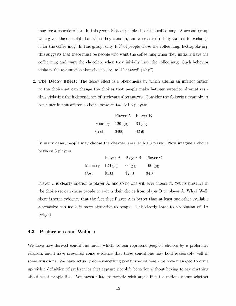
2. The Decoy Effect: The decoy effect is a phenomena by which adding an inferior option

to the choice set can change the choices that people make between superior alternatives -

thus violating the independence of irrelevant alternatives. Consider the following example. A

consumer is first offered a choice between two MP3 players

Player A Player B

Memory 120 gig 60 gig

Cost $400 $250

In many cases, people may choose the cheaper, smaller MP3 player. Now imagine a choice

between 3 players

Player A Player B Player C

Memory 120 gig 60 gig 100 gig

Cost $400 $250 $450

Player C is clearly inferior to player A, and so no one will ever choose it. Yet its presence in

the choice set can cause people to switch their choice from player B to player A. Why? Well,

there is some evidence that the fact that Player A is better than at least one other available

alternative can make it more attractive to people. This clearly leads to a violation of IIA

(why?)

4.3 Preferences and Welfare

We have now derived conditions under which we can represent people’s choices by a preference

relation, and I have presented some evidence that these conditions may hold reasonably well in

some situations. We have actually done something pretty special here - we have managed to come

up with a definition of preferences that capture people’s behavior without having to say anything

about what people like. We haven’t had to wrestle with any difficult questions about whether

13

people will like apples more than oranges. or Ferraris more than Chryslers. We haven’t even ruled

out the possibility of them liking Miley Cyrus. All we have done is observed their choices, and said

that if they satisfy a (fairly weak) consistency condition, then we can come up with a preference

relation that captures their behavior. This is a great advantage, because if we needed to decide

what it is that people like and dislike, or what it is that makes people happy, before we could do

any economic analysis, then we wouldn’t get very far.

However, something very important has happened between sections 4.1 and 4.2 that we need

to remember. In the first case, we were treating preferences as an expression of what people

actually liked. In fact, we were treating preferences as responses to questions about what people

did like. However, in the second case, all we had to go on were the choices people make. Here,

if the necessary conditions were satisfied, we can come up with a revealed preference relation

that describes people choices. However, unless we are prepared to say that what people choose is

tautologically the same as what they like, then these concepts do not necessarily have anything to

do with each other.

Consider the following example. A consumer has to choose between different brands of washing

powder. They have no idea which brand is best, so they always choose the brand with a name that

comes first alphabetically. Such a consumer will satisfy the independence of irrelevant alternatives

(check that you agree with this), and so we can generate a revealed preference relation that matches

their choice. However, it would be odd to say that the consumer is always choosing the washing

powder that they like the most.

Does this distinction matter? Well, it depends what we are using our models for. If we only want

to use them for positive purposes, then we may not care: these preferences explain the choices

that people make, and that is all we want to do. However, in many cases, economists will slip into

using their models normatively - using them to say that a particular policy is ‘good’, or ‘optimal’.

When they do so, they are almost always assuming that the optimal thing for an individual is the

thing that maximizes their preferences (or utility) - by which they mean the revealed preferences

that come from choice. We are going to fall into this trap ourselves.

Is this a valid thing to do? To me, this is a very difficult question, and one to which I have

not seen a compelling answer. Is it meaningful to say that you ‘like’ option A but choose option

B? Even if we do think revealed preference is the same as preference, is this what we should be

14

setting policy to maximize? What about drug addicts, or just people that make mistakes in their

reasoning? These are questions you will have to make up your own mind about, but you should

bear them in mind as soon as I start describing something as ‘optimal’.

4.4 Indifference Curves and the Marginal Rate of Substitution

Having spent some time discussing the nature of preferences, and whether there are such things as

well behaved, we are now going to proceed on the assumption that there our consumer does have

well behaved preferences. In this section we will learn how to describe preferences in the commodity

space that we introduced is section 3

Ideally we would like to be able to use three dimensional graphs in order to represent preferences

in the commodity space: For any consumption bundle, we would like to use the third, ‘vertical’

axis to represent preferences, with higher levels used to represent more preferred options. Figure 7

shows an example of such a graph for a particular set of preferences.

However, three dimensional graphs tend to be difficult to work with, so instead we translate the

three dimensions into two in the ways that cartographers have for years: by using isoquants. An

isoquant is a line on a graph that links points that are equal in some way. On a map, contour lines

link areas of equal height. Here, we will use indifference curves to link areas of equal preference

- or linking bundles that are indifferent. Figure 8 translates the preferences of figure 7 to two

dimensions.

What can we learn from indifference curves? Well, the first thing we can read is the marginal

rate of substitution (MRS) of one good for another. This is defined as the rate at which one

good can be traded for another while keeping the consumer indifferent. To understand this concept,

look first at figure 9. Think first of a consumer that currently has bundle (1 2). One question

we could ask is the following: Imagine we give the consumer some more of good 1, moving them

to 1 - a change that we will call ∆1. The how much of good 2 would we have to take away from

them in order to keep them just indifferent between the two points. We can read off the answer

from the indifference curve: The bundle that is indifferent to (1 2) with 1 is (1 2). Thus, to

keep the consumer indifferent, we would have to reduce the amount of consumption of good 2 to

2, a change that we call ∆2. The ratio of the increase in good 1 to the decrease in good 2 that

is needed to keep the consumer indifferent is given by the red chord in figure 9, and is equal to

15

∆2∆1

Now imagine that we make ∆1 smaller and smaller, and keep track of the ∆2 that keeps the

consumer indifferent. This is the process shown in figure 10. In the limit, the slope of the chord

connecting the indifferent point will be equal to the slope of the indifference curve at (1 2). It is

this slope that we call the marginal rate of substitution at (1 2). It is the instantaneous rate at

which the two goods can be traded off with each other to keep the consumer indifferent.

This process should look familiar to you all from your calculus class. And for the maths jocks

amongst you, we can define the MRS in a similar way.

(1 2) = − lim∆1→0

∆2

∆1

such that (1 2) ∼ (1 +∆1 2 +∆2)

4.5 Types of Preferences

We now move on to use indifference curves to describe different types of preferences. We begin by

describing two further assumptions that economists usually make about preferences. The first is

that people’s preferences are monotonic. This basically means that people like more stuff rather

than less. If we compare two bundles (1 2) and (1 2) such that 1 is at least as big as 1 and 2

is at least as big as 2 then (1 2) should be at least as good as (1 2). We say that preferences

are strictly monotonic if in addition it is the case that if one of those relations is strict (i.e. either

1 is bigger than 1 or 2 is bigger than 2) then we assume that (1 2) is actually preferred to

(1 2). Mathematically, we can write

if 1 ≥ 1 and 2 ≥ 2 then

(1 2) Â (1 2) or (1 2) ∼ (1 2)

for monotonicity, and

if also either 1 1 or 2 2 then

(1 2) Â (1 2)

for strict monotonicity.

Monotonicity implies three things about indifference curves

16

1. They are downward sloping

2. They are cannot cross

3. Moving in a ‘North Easterly’ direction in the commodity space moves to more preferred

indifference curves.

You should check that you understand all three of these properties. Figure 11 gives an example

of monotonic indifference curves.

Is monotonicity a good assumption? Well, one thing you might worry about is things that

you actively dislike (Miley Cyrus CDs), and so would actually like fewer of. But this is not

really a problem - we can just redefine the good as 1-(number of Miley Cyrus CDs), and we have

monotonicity again. A more serious problem is satiation. I certainly prefer having 1 cheeseburger

to 0 cheeseburgers, and 2 cheeseburgers to 1 cheeseburger, but do I really prefer 11 cheeseburgers to

10?. At best, I am probably indifferent (a violation of strict monotonicity) At worst I may actually

prefer 10 cheeseburgers to 11, as 11 make me feel sick (a violation of monotonicity). Thus, it is not

always the case that monotonicity is a good assumption.

Another property that economists often assume is convexity. To understand convexity. Think

of the following question. Say you are in a bar, and you currently have 10 drinks lined up in front

of you, but only 2 sliders. How many drinks would you give away in order to get another slider?

Now say you had 2 drinks and 10 sliders. How many drinks would you now exchange for a slider?

In general, we would expect people to give away more drinks in exchange for a slider when they

have a lot of drinks relative to the number of sliders. In other words, we would expect the MRS of

sliders to drinks to be higher when you have a lot of drinks than when you have a few drinks.

In terms of our indifference curves, convexity implies that curves get flatter as we move along

them: When you have a small amount of good 1, you need a lot of good 2 in return for giving some

of it up to keep you indifferent. However, when you have a lot of good 1, you need relatively little

of good 2 in return for giving up good 1 to keep you indifferent. Figure 12 shows this property of

convex indifference curves, while figure 13 gives an example of non-convex indifference curves.

One implication of convexity7 is that the average of two bundles of goods between which the

consumer is indifferent is at least as good as either of the bundles themselves. We can say that

7 In fact, this is how convexity is defined

17

preferences are convex if the following is true

For any two bundles (1 2) ∼ (1 2)

and number between 0 and 1

(1 + (1− )1 2 + (1− )2) Â (1 2) or

(1 + (1− )1 2 + (1− )2) ∼ (1 2) and

We will say that preferences are strictly convex if the average of the two is preferred to either

of the goods.

We conclude this section by introducing two types of preferences which act as the two extremes

of the set of monotone, convex preferences. The first is what we call perfect substitutes. The

easiest way to think about perfect substitutes is with an example. Say that the two goods in our

commodity space are different types of bottled water: Dasani and Aquafina. Say that all you care

about is the total number of bottles of water you have (this is all you should care about, they are

both just tap water). What would your preferences look like? Well, how many bottles of Dasani

would I have to give you in exchange for a bottle of Aquafina to keep you indifferent? If all you

care about is the total number of bottles, then the answer is 1, regardless of how many bottles

of Dasani you already have. Thus, your MRS (and thus the slope of the indifference curve) is -1

everywhere. - your indifference curves are straight lines! This is demonstrated in figure 14. Note

that these preferences are convex, but not strictly convex.

At the other extreme, we have goods we call perfect compliments. Again, we can illustrate

perfect compliments with an example. Think of good 1 as being left shoes and good two as being

right shoes. Say that all you care about is the total number of pairs of shoes (which is again

what you should care about, unless you are a shoe fetishist, or have one or three feet). What do

your preferences look like? In order to answer this question, lets think about all the points in the

commodity space in which you have exactly 2 pairs of shoes. One obvious point is the one where

you have 2 left and 2 right shoes. However, it is also when you have 2 left and 3 right shoes, 2 left

and 4 right shoes and so on. Also when you have 2 right and 3 left, 2 right and 4 left and so on. If

you graph all these points, you will see you get an ‘L’ shaped graph like the ones shown in figure

15. These are the indifference curves for perfect compliments.

18

5 Utility Functions

So far we have been representing the preferences of our consumer with the  relation. This is all

very well and good, but we want to describe the behavior of a consumer who chooses in order to

maximize their preferences. It is much easier to think about maximizing a numerical function than

it is to think about maximizing a set of binary relations. Thus, we want to know the answer to the

following question:

Question: Under what circumstances can we find a numerical function that represents the

preferences of our consumer? By represent we mean that

(1 2) (1 2) if and only if (1 2) Â (1 2)

Amazingly, (or perhaps not that amazingly). The answer is that we can find such a function if

(and only if) the preferences are complete and transitive.8

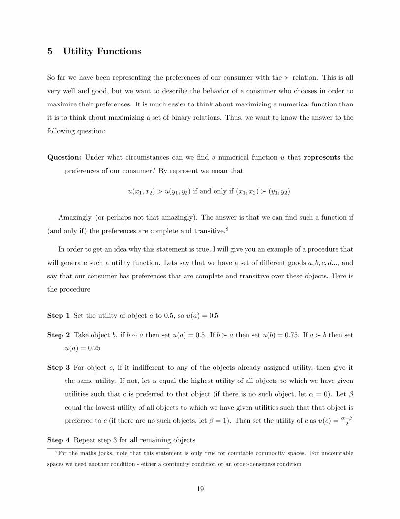
In order to get an idea why this statement is true, I will give you an example of a procedure that

will generate such a utility function. Lets say that we have a set of different goods , and

say that our consumer has preferences that are complete and transitive over these objects. Here is

the procedure

Step 1 Set the utility of object to 0.5, so () = 05

Step 2 Take object . if ∼ then set () = 05. If  then set () = 075. If  then set

() = 025

Step 3 For object , if it indifferent to any of the objects already assigned utility, then give it

the same utility. If not, let equal the highest utility of all objects to which we have given

utilities such that is preferred to that object (if there is no such object, let = 0). Let

equal the lowest utility of all objects to which we have given utilities such that that object is

preferred to (if there are no such objects, let = 1). Then set the utility of as () = +2

Step 4 Repeat step 3 for all remaining objects

8For the maths jocks, note that this statement is only true for countable commodity spaces. For uncountable

spaces we need another condition - either a continuity condition or an order-denseness condition

19

It is clear that our procedure works in step 2. To show that it works at step 3, assume that

 so () = 05 and () = 025 (you can check that this works in the other cases as well).

There are now 5 possibilities

1. Â . In this case = 1 and = 05, so () = 075. Note that, by transitivity, this implies

that  , so our function works

2. ∼ . In this case () = 05. Note that, by transitivity, this implies that  , so our

function works

3.  and  . In this case = 05 and = 025, so () = 0375

4. ∼ In this case () = 025. Note that, by transitivity, this implies that  , so our

function works

5. Â . In this case = 025 and = 0, so () = 0125. Note that, by transitivity, this

implies that  , so our function works

You should convince yourself that only one of these possibilities can occur - for example it is

impossible for  and  by transitivity.

So step 3 works. To show that step 4 also works is beyond the scope of this course, as it relies

on a proof by induction (which basically means assuming that it works with objects and showing

it works with + 1 objects).

So, assuming that we have a complete and transitive9 preference ordering, then we now have

our utility function. Great! However, it is very important to remember that the utility function

cannot tell us any more than the original preference ordering. By this I mean that the utility

function can tell us whether one object is preferred to another, but it cannot tell us any more than

that. For example, it cannot tell us things like one good is twice as good as another good - even

if the utility of one good is twice as large as another.

Why is this? Well, remember, all the utility function is doing is representing the original

preferences. And if I currently have a utility function in which () is twice as high as (), I can

9assuming we have countability

20

always pick another one that represents the preferences just as well in which the utility is four

times as high as (). To see this, define another utility function such that for every object ,

() = () − 23(). Does this new function represent the original preferences? Sure! Say  .

As the utility function represented these preferences, then this implies that () (). But now

subtract 23() from each side. The inequality still holds, so

()− 23() ()− 2

3()

so

() ()

But now

() = ()− 23() =

1

3()

while

() = ()− 23()

= 2()− 23()

=4

3()

So now the utility of (as measured by ) is 4 times as high as that for .

More generally, if we have one utility function that represents a set of preferences, then any

strictly increasing transform of that utility function will also represent those preferences. A

monotonic transformation of a function () is another function (()) such that () is strictly

increasing. Thus adding or subtracting things from a utility function, or multiplying it by a positive

number, or taking logs, will still mean it is the same utility function!

The next thing we can think about is what sort of utility function represents the preferences

we have come across in the above section. Remember, these are functions that will take as their

input the amount of good one and amount of good two that the consumer consumes, so (1 2)

It should be pretty obvious that monotonic preferences should be represented by monotonic utility

function: That is that utility should be increasing in both good 1 and good 2. If we add an amount

to good 1 and to good 2 such that ≥ 0 and ≥ 0 then utility cannot go down

(1 + 2 + ) ≥ (1 2)

21

Furthermore, for strictly monotonic utility functions, if either 0 or 0 then utility has to

be strictly higher

(1 + 2 + ) (1 2)

Convex preferences are (somewhat confusingly) represented by a utility function that is quasi

concave. This means that, for any 1 2, the set of points 1 2 such that (1 2) ≥ (1 2) is

convex (if this definition doesn’t mean very much for you, don’t worry. That is one for the maths

jocks)

What about perfect substitutes? Well, these were goods such that all the consumer cared about

was the total number of the two good (remember, the total number of bottles of water). Thus,

(1 2) Â (1 2) if and only if 1 + 2 1 + 2. We can therefore use this for a utility function

for this type of goods10

And perfect compliments. Well, here we said that the consumer only cared about the total

number of completed pairs of good 1 and good 2 they could make. This implies that their preferences

are governed by the smaller of good 1 and good 2. We can therefore represent their preferences by

the function (1 2) = min(1 2)

A final class of interesting utility functions are called the Cobb-Douglas utility functions. These

are utility functions of the form

(1 2) = 12

where and are positive numbers less than or equal to 1. You will learn to love Cobb-Douglas

utility functions, as they are very easy to work with. For a start, they represent preferences that

are monotone and convex (check)! Therefore many economists (and exam setters) choose to work

with them. Figure 15 shows a graph of the indifference curves for (1 2) = 12

1 12

2 for different

levels of utility.

Now that we have defined the concept of utility, we can define the concept of marginal utility

This measures the rate at which utility increases as we increase the amount the consumer has of

10 In fact, we use perfect substitutes more generally to denote any preferences that can be represented by a utility

function of the form 1 + 2

22

a particular good.11 It is defined as the partial derivative of the utility function with respect to

that good. We will use 1(1 2) to denote the marginal utility with resect to good 1 when the

consumer has the bundle 1,2

1(1 2) =(1 2)

1

For a Cobb Douglas utility function, we can see that

1(1 2) =(1 2)

1

=1

2

1

= (−1)1

2

A few things to note about this

1. It is positive: So as we give the consumer more of good 1, their utility goes up. This shows

that the preferences represented are monotonic

2. For a fixed 2, marginal utility is decreasing in 1. That is, as we increase the amount of

1 the consumer has, the less happy an additional unit of 1 will make them

3. For a fixed 1, marginal utility is increasing in 2. That is, as we increase the amount of 2

the consumer has, the more happy an additional unit of 1 will make them

2 and 3 together follow from the fact that Cobb-Douglas preferences are convex.

Marginal utility is related to the concept of the MRS. To see this, remember that the MRS is the

slope of an indifference curve. The one thing we know about indifference curves is that every point

on it has the same utility (yes?). Therefore, lets take the total derivative of the utility function

with respect to both 1 and 2

(1 2) =(1 2)

11 +

(1 2)

22

But, if we are moving along an indifference curve, then (1 2) = 0. Thus, we can rearrange

the above expression

11 If you followed the previous discussion, then the concept of marginal utility should be making you a bit nervous.

Given that utility functions are not unique, how much can we trust marginal utility? Could we arbitrarily double

marginal utility? Could we change its sign?

23

0 =(1 2)

11 +

(1 2)

22

⇒ (1 2)

11 = −(1 2)

22

⇒ 2

1= −

(12)1

(12)2

Thus, the marginal rate of substitution between two goods is equal to the ratio of the marginal

utilities of those two goods.

24

6 Optimal Choice

We have now set up the three elements of the consumers optimization problem:

Choose: a consumption bundle

In order to maximize: preferences (or utility)

Subject to: the budget constraint.

In this section we will think about the tools that we need to solve the optimization problem,

and therefore complete our model of consumer behavior. To start with, we will think about the

problem intuitively, and then we will show how we can use the tools of calculus to find the solution.

For the purposes of this section, we will concentrate on preferences that are monotonic. This

means we know that indifference curves get ‘better’ (i.e. represent more preferred objects) as we

move in a North-Easterly direction in the commodity space. The problem of choosing a consumption

bundle in order to maximize preferences is therefore the same as choosing a consumption bundle

on the most North-Easterly indifference curve possible.

What is such an optimal bundle going to look like? There are two possibilities, which we will

illustrate by examples. First, let us go back to the example of perfect substitutes. In particular,

lets assume that the preferences of consumers can be represented by

(1 2) = 1 + 22

And let us assume that the price of goods is 1 for good 1 and 1 for good 2, and the consumers

income is 10. The consumers problem is therefore

Choose: a consumption bundle (1 2)

In order to maximize: (1 2) = 1 + 22

Subject to: 1 + 2 ≤ 10

This budget constrain and indifference curves are illustrated in figure 16. The slope of the

budget line is −12= −1, while the slope of the indifference curves is always −1

2. The indifference

curves are therefore flatter than the budget constraint. What is the optimal consumption bundle

25

for this consumer? Well, remembering that the optimal point is that which gets the consumer onto

the most North-Easterly indifference curve, it should be clear that it is optimal for the consumer

to spend all of their money on good two. A quick examination of figure 16 will show that the

indifference curve going through the point (0 10) is the best that the consumer can obtain This

indifference curve is clearly obtainable (by consuming (10 0), which is affordable). Moreover, it

is better than all the indifference curves below it, and all the indifference curves above it are

unobtainable. We call such a solution a corner solution because it occurs at one corner of the

budget constraint.

We should also be able to convince ourselves that this is the best bundle for the consumer in

the following way: We know that the consumer can trade off goods in the market at a ratio of

1 to 1: If they consume one less unit of good one they can consume one more unit of good two.

However, the marginal rate of substitution along the indifference curve is 12(note that it is only

because these goods are perfect substitutes that the MRS is a constant): this means that to keep

the consumer indifferent, they would only have to give them half a unit of good 2 in return for a

unit of good 1 in order to keep them indifferent. Thus, if the consumer is currently consuming any

units of good 1, they could always trade that in for more good two and make themselves happier.

It is therefore can only be optimal for the consumer to spend all their money on good 2.

Next we consider the case of perfect compliments. Remember, these are good that can be

represented by a utility function such as (1 2) = min(1 2). In this case, let us assume that

the the price of good one is 1, the price of good two is 2 and the consumer again has income 10.

The optimization problem is now

Choose: a consumption bundle (1 2)

In order to maximize: (1 2) = min(1 2)

Subject to: 1 + 22 ≤ 10

This example is illustrated in figure 17. Now what is the optimal bundle for the consumer to

consume? From figure 17, it should be clear that the optimal point is for the consumer to consume

an equal proportion of good one and good two: the highest indifference curve that they can get on

is the one which touches the budget constraint, but does not cross the budget line. This occurs at

the ‘kink’ in the indifference curves, where 1 = 2. Knowing this, we can use the budget constraint

26

to solve explicitly for 1 and 2

1 + 22 = 10

1 + 21 = 10

1 =10

3= 2

We call this type of solution, where the consumer consumes strictly positive amounts of both

good an interior solution.

Again, we should be able to see intuitively that for this example the solution is for the consumer

to consume the same amount of both goods. Say that the consumer wasn’t doing this and was (for

example) consuming more of good one than good two. Then the consumer could consume less of

good one without making themselves any worse off. By consuming less of good one, they could buy

more of good two, which would make them better off, as (1 2) = min(1 2). Thus, the only

case where the consumer cannot make themselves better off is where they are consuming exactly

the same amount of good one and good two.

6.1 The Tangency Condition

So far we identified the two possible types of solutions we might find for the optimization problem:

interior solutions and corner solutions. In general this may not tell us very much. However, this is

a very useful differentiation in the case where the consumer’s indifference curves are differentiable.

For the purposes of this course, we can think of a differentiable function as one that is ‘smooth’,

in the sense that it has a unique tangent (and therefore unique slope) at any point. Of all the

functions that we have come across so far, the only one that is not differentiable is min(1 2). As

figure 18 shows, this function does not have a unique slope at its kink.

The interesting property of interior solutions for differentiable functions is that, at any such

solution, the slope of the indifference curve has to be the same as that of the budget

line - in other words they are tangent. This is an incredibly useful property, and one that you

can see this from figure 19. This shows two points at which the budget line is not tangent to the

indifference curves - (1 2) and (1 2) - and one where it is - (1,2). If we look at (1 2), it

is clear that this is not an optimal consumption bundle - the consumer could move onto a higher

indifference curve by swapping good 1 for good 2 - i.e. by moving down the budget constraint.

27

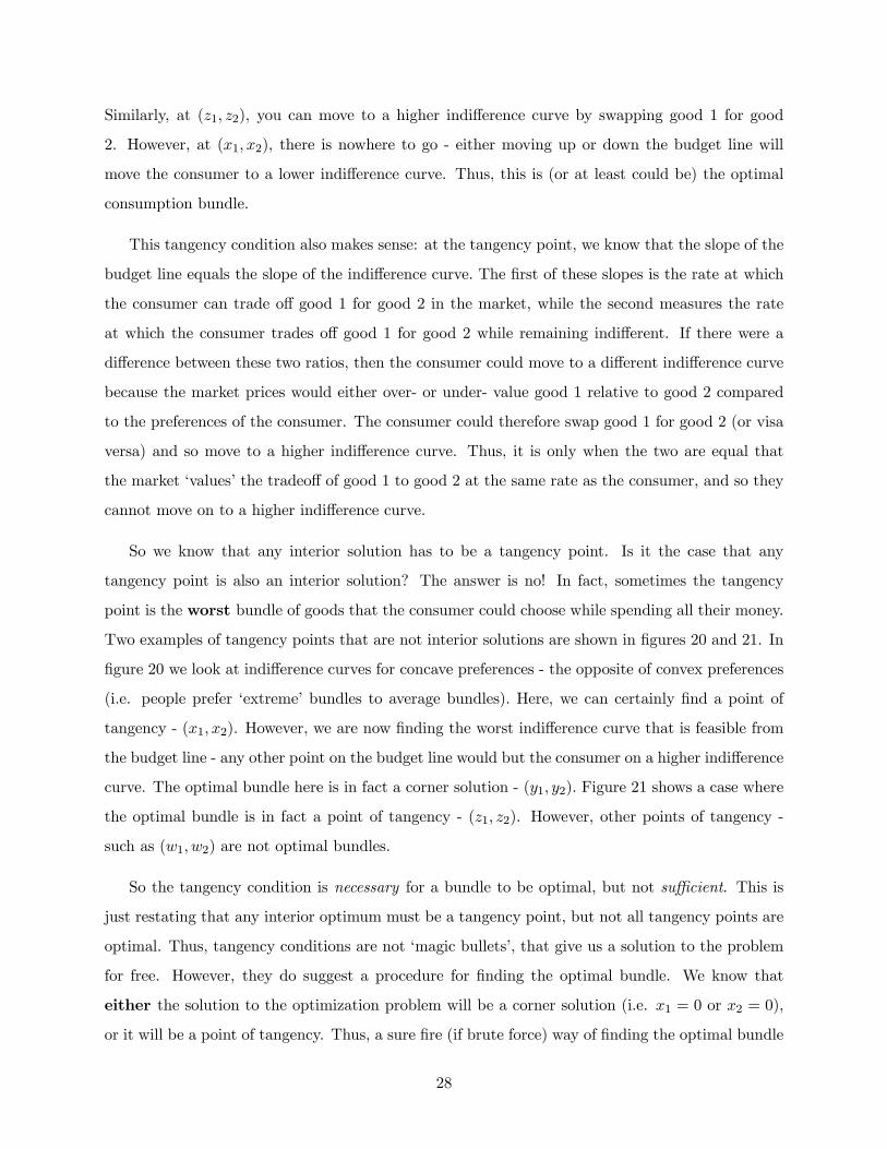
Similarly, at (1 2), you can move to a higher indifference curve by swapping good 1 for good

2. However, at (1 2), there is nowhere to go - either moving up or down the budget line will

move the consumer to a lower indifference curve. Thus, this is (or at least could be) the optimal

consumption bundle.

This tangency condition also makes sense: at the tangency point, we know that the slope of the

budget line equals the slope of the indifference curve. The first of these slopes is the rate at which

the consumer can trade off good 1 for good 2 in the market, while the second measures the rate

at which the consumer trades off good 1 for good 2 while remaining indifferent. If there were a

difference between these two ratios, then the consumer could move to a different indifference curve

because the market prices would either over- or under- value good 1 relative to good 2 compared

to the preferences of the consumer. The consumer could therefore swap good 1 for good 2 (or visa

versa) and so move to a higher indifference curve. Thus, it is only when the two are equal that

the market ‘values’ the tradeoff of good 1 to good 2 at the same rate as the consumer, and so they

cannot move on to a higher indifference curve.

So we know that any interior solution has to be a tangency point. Is it the case that any

tangency point is also an interior solution? The answer is no! In fact, sometimes the tangency

point is the worst bundle of goods that the consumer could choose while spending all their money.

Two examples of tangency points that are not interior solutions are shown in figures 20 and 21. In

figure 20 we look at indifference curves for concave preferences - the opposite of convex preferences

(i.e. people prefer ‘extreme’ bundles to average bundles). Here, we can certainly find a point of

tangency - (1 2). However, we are now finding the worst indifference curve that is feasible from

the budget line - any other point on the budget line would but the consumer on a higher indifference

curve. The optimal bundle here is in fact a corner solution - (1 2). Figure 21 shows a case where

the optimal bundle is in fact a point of tangency - (1 2). However, other points of tangency -

such as (1 2) are not optimal bundles.

So the tangency condition is necessary for a bundle to be optimal, but not sufficient. This is

just restating that any interior optimum must be a tangency point, but not all tangency points are

optimal. Thus, tangency conditions are not ‘magic bullets’, that give us a solution to the problem

for free. However, they do suggest a procedure for finding the optimal bundle. We know that

either the solution to the optimization problem will be a corner solution (i.e. 1 = 0 or 2 = 0),

or it will be a point of tangency. Thus, a sure fire (if brute force) way of finding the optimal bundle

28

is to list all such points (i.e. all points of tangency and all corner solutions) and determine which is

the best of those bundles. Unless you have a reason for a priori ruling out some possible solutions

to the optimization problem, then this is the approach you should take to solving the problem

One case in which tangency conditions are both necessary and sufficient is when preferences

are strictly convex - for example those which are represented in figure 19. An examination of this

graph should tell you the following facts12

1. There can be at most one tangency point between strictly convex, monotone preferences and

the budget constraint

2. Such a point must be a maximum

This is one of the reasons that economists love convex preferences so much! Though note there

is still one slight issue - even with a convex function, there may be no points of tangency (this is a

homework hint for those who are staying awake), in which case the solution to the problem will be

a corner solution.

6.2 Locating Tangency Points

All this is very well and good, but knowing about tangency conditions is not very helpful if we

don’t know how to locate them. Luckily, this is where we can use some of the machinery that

mathematicians have developed - in particular the tools of calculus. This is one of the reasons that

we went to all the effort of deriving a numerical utility function to start with.13

Remember a point of tangency is a point at which the slope of the budget line equals the slope

of the indifference curve. We know exactly what the slope of the budget line is: it is just the ratio

−12. However, we have also discussed how to find the slope of the indifference curve. Remember

that this is marginal rate of substitution of one good for another. Furthermore, we have already

established the result that the MRS of two goods is the ratio of the marginal utility with respect

to those two goods. This gives us the following result

12Which we can also prove, but this goes beyond the scope of this course13Though, maths jocks, note that we have not discussed conditions that guarantee the existence of a differentiable

utility function, so I am taking some liberties here.

29

Result 1 A bundle (1 2) is a point of tangency between the budget line and an indifference

curve if

−12= −

(12)1

(12)2

= −1(1 2)

2(1 2)= −(1 2)

and so

1

2=

(12)1

(12)2

=1(1 2)

2(1 2)=(1 2)

The tools of calculus also give us a way to determine whether people have strictly convex

preferences An examination of figure 17 shows us that the defining characteristic of strictly convex

preferences is that the marginal rate of substitution decreases along the indifference curve as 1

increases. At low 1 the consumer will trade a lot of 2 for a little 1, while at high 1 they will

trade a lot of 1 for little 2. Thus, the slope of the indifference curve must be flattening as 1

increases - or becoming less negative. This means that the second derivative of the indifference

curve must be positive. This will become more clear with the following example.

6.3 An Example: Cobb Douglas Preferences

We now put this all together to solve for the optimal bundle in the case of Cobb Douglas preferences.

We will assume that the utility of the consumer is given by (1 2) = 121

122 We will also assume

that 1 = 3, 2 = 4 and = 15. The consumer’s problem is therefore

Choose: a consumption bundle (1 2)

In order to maximize: (1 2) = 121

122

Subject to: 31 + 42 ≤ 15

The approach that we are going to take is to start by finding any point of tangency between the

budget line and the indifference curve. We know that, from result 1, this will be a point at which

1

2=

(12)1

(12)2

So we need to calculate the marginal utility with respect to 1 and 2

(1 2)

1=

1

212−11

12

2 =1

2− 12

1 12

2

(1 2)

2=

1

2121 −12

2

30

Now, something quite handy is going to happen when we take the necessary ratio

(12)1

(12)2

=12− 12

1 122

1212

1 − 12

2

=2

1

Another magic property of the Cobb Douglas utility function!.

We therefore know that a point of tangency will occur when

3

4=

2

1

or

2 =3

41

Well, this is okay but we have only got 2 as a function of 1. This is not surprising, as we

have not so far ‘told’ the procedure which budget line we are on - or what the income is. We can

therefore substitute this relationship into the budget constraint:

31 + 42 = 15

⇒ 31 + 4

µ3

41

¶= 15

⇒ 31 + 31 = 15

⇒ 1 =15

6

and so 2 =158

But is this the solution to the optimization problem? Well, we know that this is the only

tangency point, as it is the only solution to the above system of equations. But what about corner

solutions? Well, looking at the utility function, we can see that spending all the money on good 1

or all the money on good 2 is a bad idea:

(015

4) = 0

12

µ15

4

¶ 12

= 0 = (5 0)

so it must be that the tangency point is the optimum bundle.

In fact, we didn’t need to do this last step, as Cobb Douglas preferences are strictly convex. To

see this, take some level of utility , and note that the indifference curve related to this utility level

31

is given by

= 121

122

or

121

= 12

2

2 =2

1

The first derivative of this function is

2

1= −

2

21

While the second derivative is

22

21= 2

2

31

Which is positive. The slope of the indifference curve is therefore increasing (becoming less

negative) as 1 increases, which is how we characterized convex preferences!

Congratulations! You have just solved your first ‘standard’ economics optimization problem.

You will be absolutely amazed how many more problems of this type I will force you to solve.

Just to reiterate, the steps we went through to solve this problem are as follows:

1. Solve for the marginal utilities(12)

1and

(12)2

2. Use the tangency condition 12=

(12)

1(12)

2

to get an expression for 1 as a function of 2

3. Substitute this expression into the budget constraint to get an explicit solution for 1 and 2

(as a function of the parameters of the problem: 1, 2 and )

4. Check that the tangency solutions are better than the corner solutions

For completeness, it is worth noting that there is another way of solving this problem. Seeing

as preferences are monotonic, we know that the consumer will always spend all their money. This

means that if we know what 1 is we know what 2 is, as

31 + 42 = 15

⇒ 2 =15

4− 341

32

Thus, we can substitute this into the utility function, which is now only a function of 1

(1 2) = 12

1 12

2

= 121

µ15

4− 341

¶12

This is now an unconstrained optimization problem, so we can differentiate with respect to 1

and set that equal to zero to find the critical points

112

1

µ15

4− 341

¶ 12

=1

2−12

1

µ15

4− 341

¶ 12

− 38121

µ15

4− 341

¶− 12

= 0

so

1

2− 12

1 121

µ15

4− 341

¶ 12

=3

8121

µ15

4− 341

¶− 12

which gives

15

4− 341 =

6

81

1 =15

6

The same answer as the other approach! Of course, this approach doesn’t excuse you for

checking that this solution is better than the corner solutions.

6.4 The Dual Problem

Before we go on, we need to introduce a problem closely related to the consumer’s optimization

problem: This is the expenditure minimization problem. So far we have asked the question:

Assume that the consumer has a fixed budget constraint: What is the maximum utility they can

achieve given their income:

The consumer’s optimization problem

Choose: a consumption bundle (1 2)

In order to maximize: (1 2)

Subject to: 11 + 22 ≤

33

A closely related problem is the following: Imagine that the consumer has to achieve a fixed

level of utility: What is the least expensive way for them to do this? The dual problem is defined

as

The consumer’s dual problem

Choose: a consumption bundle (1 2)

In order to minimize: 11 + 22

Subject to: (1 2) =

For the consumer’s problem, we fixed a budget line and asked what the highest indifference

curve that the consumer could obtain. The dual problem fixes an indifference curve, and asks what

the smallest budget constraint can obtain that utility (assuming fixed prices).

It seems like the solution to these two problems should be related: in particular it seems like

the tangency results we derived for the consumer’s optimization problem should also hold for the

dual problem. And in fact this is the case - assuming we have monotonic preferences14. In this

case, the following is true:

Result 2 Say a bundle (1 2) solves the consumer’s problem: it maximizes (1 2) subject to

11 + 22 ≤ , and utility (1 2) = ∗. If preferences are monotonic, then (1 2) also

solves the dual problem: it minimizes 11 + 22 subject to (1 2) = ∗. Moreover, the

minimum expenditure is

This somewhat pointless-seeming exercise is going to come in very useful in the next section.

14Maths jocks: we also need continuity here

34

7 The Demand Function

Now we know how to solve the consumer’s problem, which is great: If we know (or are prepared

to make assumptions about) a consumer’s preferences (represented by a utility function), we can

figure out what consumption bundle they will choose from a given budget set. In this section we

will look at how this optimal bundle - the bundle that the consumer chooses - depends on the

properties of that budget set.

Have another look at the budget set

11 + 22 ≤

The set is defined by three parameters: 1, 2 and 15 These are things that the consumer

cannot control (they do not get to choose the prices or income they receive), but they clearly can

affect what it is that the consumer will choose. In other words, the bundle that the consumer

chooses will depend of the values of these things. This relationship is captured by what we call the

demand function, which we write as

∗1(1 2)

∗2(1 2)

This is the amount of good 1 and good 2 that the consumer will choose if they face prices 1, 2

and . In other words, (∗1(1 2) ∗2(1 2)) is the solution of the consumer’s optimization

problem:

The consumption bundle (∗1(1 2) ∗2(1 2)) maximize (1 2) subject

to the budget constraint 11 + 22 ≤

Clearly, firms, policy maker and so on are going to want to know about the properties of these

functions: how does demand for a particular good change as the price of that goes up? What about

when people get richer? These are the questions we are going to ask in this section: how do the

consumer’s optimal bundles change as the parameters of the consumer’s problem change?

15Though remember that we have said that we can forget about one of these parameters - look at the end of section

3

35

7.1 The Relationship between Demand and Income.

We are first going to think about how demand for a particular good depends on , or income -

assuming that prices stay constant. As has been our tradition, we will start out by thinking about

two specific examples - perfect substitutes and perfect compliments.

First, let’s derive the demand function for perfect substitute preferences. Remember that the

consumer’s problem for perfect substitutes is

Choose: a consumption bundle (1 2)

In order to maximize: (1 2) = 1 + 2

Subject to: 11 + 22 =

Recall from section 6 that the optimal thing for the consumer to do is to spend all of their

money on good one if the price of good one is less that the price of good two, and spend all of their

money on good two otherwise. What about the case where the price of good one is equal to good

two? Well, in the case the consumer’s utility will be the same whatever they choose to consume -

as long as they spend all their money (check that you agree with this statement). We can therefore

only make very weak predictions in this case: we know that the consumer cannot spend less that 0

on either good, and we know that they can’t spend more that 1on good one or

2on good two,

but beyond that we don’t know very much. Thus, we have to think about three cases

∗1(1 2) = 0 if 1 2

=

1if 2 1

0 ≤ ∗1(1 2) ≤

1if 2 = 1

Using this information, we can graph how demand for good one changes with income for perfect

substitutes. Such graphs are, in general, called Engle curves. Figure 22 shows the Engle curves for

perfect substitutes under two conditions: where 1 2 and where 2 1

Mathematically, we describe how demand changes with income using the concept of the income

elasticity of demand (IED). We do this in a slightly more complicated way than might seem

obvious. Rather than just measure the rate of change of demand with respect to income - i.e.

∗1(1 2)

36

We measure how a percentage change in income leads to a percentage change in demand. The

income elasticity of demand is given by

1 =∗1(1 2)

∗1(1 2)

We will use 1 to refer to the income elasticity of demand of good 1. This formula can look a

bit mysterious. The way to think about it is as follows. Say that an % change in income leads to

a % change in demand. Then we want the IED to be %%- in other words, the percentage change

in demand is the percentage change in income multiplied by the elasticity. But

% =∆

and % =

∆∗1∗1

Thus

=

∆∗1∗1∆

rearranging this gives

=∆∗1∆

∗1

Taking the limit as ∆ goes to zero gives the formula for income elasticity for demand.

The reason for that we measure elasticity in this way is that we don’t want arbitrary changes

of units to affect elasticity. So for example, if we were to suddenly decide to measure as ‘ounces

of potatoes’ rather than ’pounds of potatoes’ then this would affect∗1(12)

but not 1

For our perfect substitutes, we can calculate IED for the case where 1 2

1 =∗1(1 2)

∗1(1 2)

=1

1

∗1(1 2)

=1

1

1=1

11 = 1

So a 1% increase in income leads to a 1% increase in consumption of good 1.

We can perform the same exercise for perfect compliments In this case, the consumer’s problem

is

Choose: a consumption bundle (1 2)

37

In order to maximize: (1 2) = min(1 2)

Subject to: 11 + 22 =

As we have demonstrated before, the best thing for the consumer to do is to buy exactly the

same amount of good 1 as of good 2, so 1 = 2. Substituting this into the budget constraint gives

11 + 21 = and so 1 =

1+2= 2. Thus the demand function is given by

∗1(1 2) =

1 + 2

Figure 23 shows the Engle curve for perfect compliments. Once again, the Engle curve is a

straight line, but here the slope is flatter than the curve for perfect substitutes (in the case where

1 2) The IED for perfect compliments

1 =∗1(1 2)

∗1(1 2)

=1

1 + 2

∗1(1 2)

=1

1 + 2

1+2

= 1

So again the income elasticity of demand is equal to 1.

In both these examples an increase in income leads to an increase in the amount consumed of

both goods. But does this have to be the case? The answer is no! Even with monotonic, convex

preferences, an increase in income can lead to a decrease in the consumption of one of the goods.

We can illustrate such a case graphically in figure 24. In this case, income increases from M to M’,

but the tangency conditions imply that this leads to a fall in the demand for good one. Moreover,

the indifference curves we have drawn are those of convex, monotonic preferences. Over this range

of income changes, the Engle curve for this good would be downward sloping.

Is such a situation likely? I would argue that it is pretty easy to think of goods that we consume

less of as we get richer. Ramen noodles spring to mind. Such goods (i.e. those with a negative

IED) are known as inferior goods. All other goods are known as normal goods.

7.2 The Relationship between Demand and a Good’s Own Price

Next, we would like to analyze how the demand for a good changes with the price of that good,

keeping the price of the other good, and income, constant. This relationship is the demand curve

38

that you may have met in Econ 011. Again, let’s begin with our old friends perfect compliments

and perfect substitutes. Recall, that for perfect substitutes, the demand function is given by

∗1(1 2) = 0 if 1 2

=

1if 2 1

0 ≤ ∗1(1 2) ≤

1if 2 = 1

The resulting demand curve (or actually the inverse demand curve, as we have switched the

axes) is shown in figure 25. For prices such that 1 2, the relationship between 1 and ∗1 is

given by 1, which looks like a downward sloping convex curve. At the point at which 1 = 2,

demand can be anywhere between 2and 0, so at this point the demand curve is a vertical line.

For any prices 1 2, demand for good one is zero. Note that for prices around 1 = 2, tiny

changes in prices can make demand ‘jump’ from 0 to 1, so in this region, demand is very sensitive

to changes in prices.

Just as we defined the concept of the income elasticity of demand, we can define the price

elasticity of demand (PED) as

1 = −∗1(1 2)

1

1

∗1(1 2)

We use 1 to refer to the price elasticity of good one. Note that, as∗1(12)

1 1∗1(12)

is

(almost) always negative, we define the PED as the negative of this value so we don’t have to carry

a minus sign around with us everywhere.

The price elasticity of demand of a good is one of its most important properties from the point of

view of an economist (and businessmen). If a good has a high price elasticity of demand, consumers

will respond a lot to changes in price, while if it has a low elasticity they will respond only a little.

Goods with 1 we call elastic, while those with 1 we call inelastic. Why is 1 important?

Think about how the amount of money, 1∗1(1 2) the consumer will spend on a good will

changes as prices change.

1(1

∗1(1 2)) = ∗1(1 2) + 1

∗1(1 2)1

39

This will be greater that zero if

∗1(1 2) + 1∗1(1 2)

1 0

⇒ −1 1

∗1(1 2)

∗1(1 2)1

⇒ 1

Thus, if a good is price inelastic, consumers will spend more on it if its price goes up, whereas

if it is elastic they will spend less on it as the price goes up.

For perfect substitutes (again, if 2 1) the price elasticity of demand for good 1 is given by

1 = −∗1(1 2)

1

1

∗1(1 2)

=

21

11

= 1

Perfect substitutes therefore have unit elasticity when 1 2. This makes sense - as the

consumer is spending all their money on good 1, a change in the price of that good will not affect

how much money they spend on that good.

Moving on to perfect compliments, here we remember that

∗1(1 2) =

1 + 2

Figure 27 shows the inverse demand curve, while the elasticity is given by

1 = −∗1(1 2)

1

1

∗1(1 2)

=

(1 + 2)2

1

(1+2)

=1

1 + 2

So good 1 will always be price inelastic, as 11+2

1. This also makes sense. As the consumer

will always buy the same amount of good 1 and good 2, an increase in the price of good 1 will lead

to an increase in spending on that good.

Again, in both these examples we have had demand falling as price increases. Do our assumptions

guarantee that? Interestingly, the answer is again no! Figure 28 demonstrates a case in which

40

monotonic, convex indifference curves can lead to demand for good 1 increasing as the price goes

up. So what the hell is going on here?

On way to think about this is that the change from 1 to 01 actually has two effects. It changes

the rate at which good one can be traded off for good two in the market place (the change in the

price ratio). But it also makes the consumer worse off, in the sense that they can no longer afford

to be on the same indifference curve. We can therefore separate out these two effects: We can ask

what the effect of the price change would be if consumers could stay on the same indifference curve,

then we could ask what effect the change in income has, resulting from the price change.

Figure 29 makes these two effects explicit, by doing the following thought experiment: First,

imagine that we change prices (increased 1) but gave the consumer an increase in income, so they

could keep on the same indifference curve. This would lead the consumer to move from A to B, and

decrease the amount they consume of good 1. We call this the substitution effect. You should

convince yourself that the substitution effect must always be negative for convex preferences.

However, we also have to deal with the fact that the price increase makes the consumer poorer

- they do not in fact, get the income increase to offset the price rise, so they will end up on a lower

indifference curve. This is the pure income effect and moves them from to . This effect could

go either way. If the good is normal, then the income effect will also act to reduce demand for good

1. However, if the good is inferior, then the effective reduction in income could lead to an increase

in demand for good 1. In extreme cases, this income effect could offset the substitution effect, and

an increase in the price of good 1 could lead to an increase in the demand for that good.

To make this formal, we need to think again about the dual problem, which (as you remember)

is

The consumer’s dual problem

Choose: a consumption bundle (1 2)

In order to minimize: 11 + 22

Subject to: (1 2) =

Here, we can define a demand function which measures how demand changes as price changes,

utility is fixed, but income may change (in contrast to the standard demand curve, which keeps

income fixed, and allows utility to change). This demand is called compensated (or Hicksian)

41

demand, which we will define as the solution to the dual problem.

(∗1(1 2 ) ∗2(1 2)) minimizes 11 + 2 subject to (1 2) =

The compensated demand is what we calculate when we go from point A to point B in figure

29. We can also define what we are going to call the expenditure function: the cost of obtaining

utility with prices 1 and 2

(1 2 ) = 1∗1(1 2 ) + 2

∗2(1 2 )

We can use these two concepts to formally break down the change in demand due to price

changes into the income and substitution effects. To see this, note that we claimed that the bundle

that solves the consumer’s problem is the same as that which solves the dual problem if we are

talking about the same indifference curve. Say we are on the indifference curve that gives utility

Then

∗1(1 2 (1 2 )) = ∗1(1 2 )

In other words, the bundle that minimizes expenditure while obtaining utility is the same as

the bundle that maximizes utility if income is equal to (1 2 ), or the amount needed to obtain

utility

Differentiating both sides of this with respect to 1 gives16

∗11

+∗1

1=

∗11

⇒ ∗11

=∗11− ∗1

1

Which already looks like we have split the effect between the substitution effect (the first term)

and the income effect (the second term). In fact, we can do better than this, because we know

something about 1

(1 2 )

1=

1(1

∗1(1 2 ) + 2

∗2(1 2 )

= ∗1(1 2 ) + 1∗11

+ 2∗21

16For convenience, we will now write ∗1 for ∗1(1 2 (1 2 )) and

∗1 for

∗1(1 2 ), but you should remember

that these are still functions.

42

The change in the expenditure function can be split into the direct effect of the change in prices

(∗1(1 2 )) and the indirect effect due to the change in the optimal bundle³1

∗11

+ 2∗21

´.

However, it turns out that, because this is the solution of an optimization problem we can ignore

the indirect effect. This is an application of the envelope theorem. To see this, notice that,

changes in compensated demand due to the change in price cannot lead to changes in utility

1=

∗1

∗11

+

∗2

∗21

= 0

But, from the tangency condition, we know that

∗2∗1

=2

1

⇒

∗2=

2

1

∗1

So we get

∗1

∗11

+

∗2

∗21

= 0

⇒

∗1

∗11

+2

1

∗1

∗21

= 0

⇒

∗1

1

1

µ1∗11

+ 2∗21

¶= 0

⇒ 1∗11

+ 2∗21

= 0

and so

(1 2 )

1= ∗1(1 2 ) = ∗1(1 2 (1 2 ))

Substituting back into the equation above gives us

∗11

=∗11− ∗1

∗1

This is the (rightfully) famous Slutsky Equation.

The change in demand with respect to a price change is the sum of the change in compensated

demand (the substitution effect), plus the income effect∗1

∗1

For an increase in prices to lead to an increase in demand it has to be the case that this

expression is positive. As∗11

is negative it must be the case that∗1

∗1 is both negative and large

43

enough to overcome the substitution effect. This gives us a hint of the type of goods for which this

might be true. First, such goods have to be inferior (as∗1

has to be negative). Second, they have

to make up a large proportion of consumption (∗1 has to be large). Such goods are called Giffen

goods.

Do such goods exist in practice? Evidence is mixed. The standard example given is that of

staple foods. Imagine that you are an ancient British peasant, and you are choosing between eating

gruel and beef. If the price of gruel goes up, then you may not be able to afford to buy beef -

but in order to keep yourself alive you need a certain amount of calories, so you buy more gruel.

Economists have spent some time looking for examples such as this, and some recent evidence from

consumption patterns in China have suggested that rice may indeed be a Giffen good under some

circumstances.

7.3 The Relationship between Demand and the Other Good’s Price

The final relationship we are interested in is the relationship between the price of good 2 and the

amount demanded of good 1: How does demand for good one change as we change the price of

good two? Intuitively, we can think of this relationship as going either way. Consider the case of

Pepsi and Coke. Here, you might expect an increase in the price of pepsi to lead to an increase in

the demand for coke. This is the case of substitutes - or goods that can be substituted for each

other. On the other hand, consider the case of golf bags and golf clubs. Here, you might expect a

rise in the price of golf clubs to lead to a fall in the demand for golf bags - if you are buying fewer

golf clubs, then you are going to need fewer golf bags as well. Such goods are called compliments.

These two words should sounds familiar - we have been banging on about perfect substitutes and

perfect compliments for this entire chapter. Figure 30 shows the relationship between ∗1(1 2)

and 2 for perfect substitutes. For 2 1 demand for good 1 is zero. For 2 1 demand for

good 1 is 1 For prices such that 1 is close to 2, then a tiny increase in the price of good two

can lead to a ‘jump’ in demand for good 1 from 0 to 1.

Figure 31 shows the same relationship for perfect compliments. Here the relationship is smoothly

downward sloping for all values of 2. In fact, the curve is exactly the same shape as the demand

curve for good 1: For perfect compliments, ∗1(1 2) responds in exactly the same way to a

change in the price of good 1 and a change in the price of good 2!

44

We can also define the elasticity of demand for good one with respect to the price of good 2.

We call the the cross elasticity of demand

21 =∗1(1 2)

2

2

∗1(1 2)

A positive number indicates that the two goods are substitutes - an increase in the price of

good 2 leads to an increase in the demand for good 1 - while a negative number means that they

are compliments.

If we look at perfect substitutes, then we will see that the cross elasticity of demand for good

1 is 0 everywhere apart from where 1 = 2 where it is (effectively) infinity! An arbitrarily small

increase in the price of good 2 will cause demand for good 1 to leap from 0 to 1. This is why

these goods are called perfect substitutes. In contrast, for perfect compliments, the cross elasticity

of demand is given by

21 =∗1(1 2)

2

2

∗1(1 2)

= −

(1 + 2)2

1

(1+2)

= − 2

1 + 2

which is (unsurprisingly) always negative.

45

7.4 Consumer Surplus

We now know how to start off with assumptions about a consumer’s preferences and make predic-

tions about their behavior in the form of a demand function. We are now breifly going to discuss

what we can learn going in the other direction - in other words what we can learn about a con-

sumer’s ‘welfare’ from their demand function. In particular, we are going to develop some measure

of how much benefit, or ‘consumer surplus’, a consumer gets from buying a particular good at a

particular price. So, for example, we want to know how much benefit does a consumer get from

being able to buy bananas for 50c each, compared to the case when they are not allowed to buy

bananas.

Informally, we want to develop the idea that the area under the demand curve for bananas tells

us something about the benefit a consumer gets from buying bananas. To get the idea, look at the

graph shown in figure 32, which shows the demand curve, but in now with price on the vertical axis

and amount on the horizontal axis. What the demand curve tells us is that, if the consumer were

to be only offered bananas, then she would happily pay price per bananaIn other words,

is her reservation price for bananas. If she were offered bananas, then here reservation price

is and so on. However, she only actually has to pay ∗ per unit. Thus, we might get the idea

that, for the first bananas the consumer consumes,. the benefit of consumption outweights the

price. This is the idea that consumer surplus tries to capture. as shown in figure 33. The triangle

A between the price line and the demand curve is what we refer to as the consumer surplus (note

that the box B is total expenditure on the good). We want to think of this as the benefit that the

consumer gets from being allowed to buy this good.

How does this idea of consumer surplus link in with the carefully constructed work on preferences

and so on that we have already done? Well, unfortunately the answer is ‘not perfectly’. However,

one case in which the two ideas do link up is in the case of quasi-linear preferences. Remember,

these are preferences are of the form

( ) = () +

so, in some sense, the consumer’s preference for is separated from there preference for : their

marginal utility with respect to is independent of the amount of they consume We can think of

this as the consumer’s preference with respect to a particular good, , (bananas), and ‘everything

46

else’ . In fact, we will think of as just amounts of money that the consumer can spend on other

goods, so the consumer’s budget constraint is

+ ≤

How much does the consumer benefit from being able to consume good ? Well, if the consumer

buys units of good at price , their utility is

() + −

whereas, if they did not consume any of good , their utility would just be (setting (0) = 0)

Thus, the added utility of being able to consume is ()− , the utility given by minus

income spent on

How does this relate to the area under the demand curve? To see this, remember that the

demand function records the consumers optimal consumption of good at each price, which,

assuming we have an interior solution, is given by

=

or, in this case

()

=

Thus, if we integrate the demand function between 0 and ∗ we getZ ∗

0

()

=

Z ∗

0

()

= (∗)

So the area under the demand cuve is equal to the total utility from consuming ∗. Thus, the

consumer surplus equals Z ∗

0

()−

47

As is the area of the box the consumer surplus is given by the triangle .

Of course, this result is specific to our choice of quazi-linear preferences, and particular the lack

of income effect. However, more generally, we can hope that the area under the demand curve gives

approximately the same result.

48

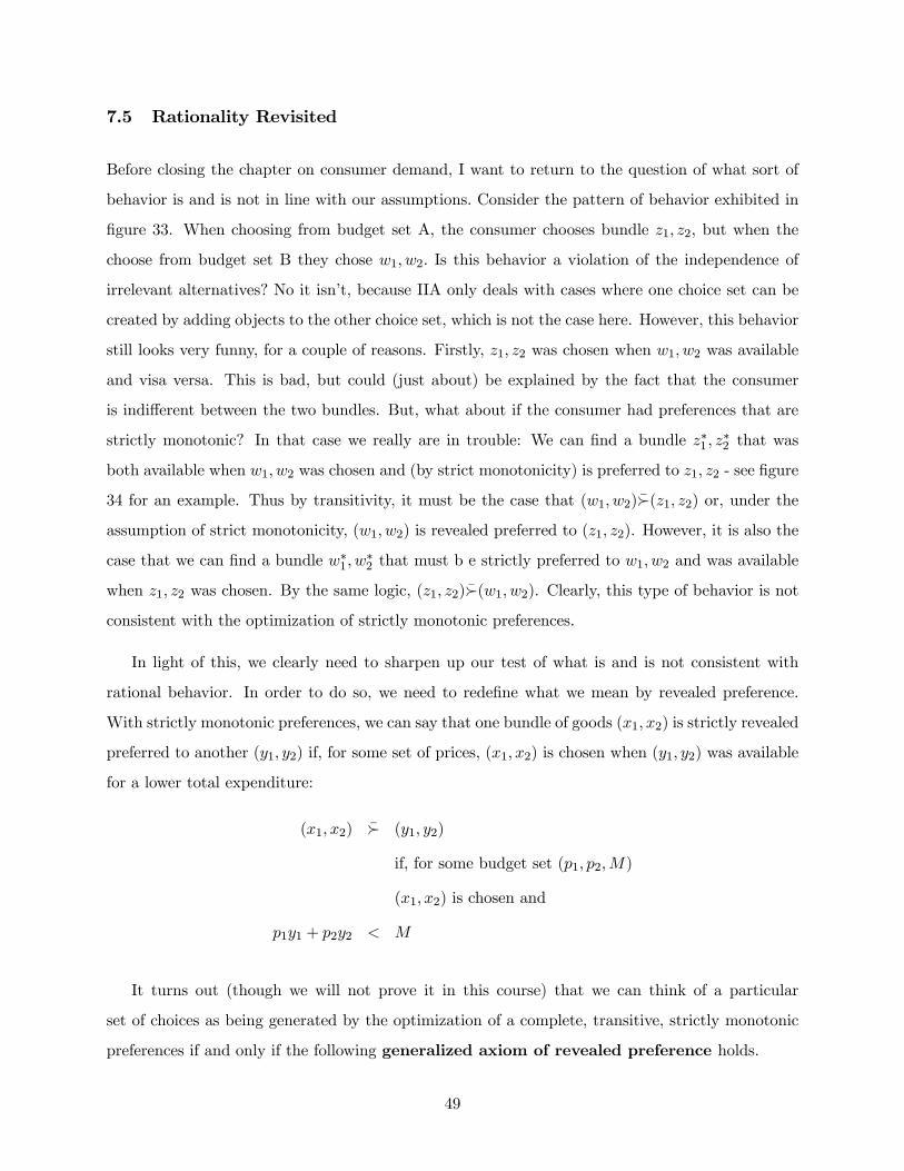
7.5 Rationality Revisited

Before closing the chapter on consumer demand, I want to return to the question of what sort of

behavior is and is not in line with our assumptions. Consider the pattern of behavior exhibited in

figure 33. When choosing from budget set A, the consumer chooses bundle 1 2, but when the

choose from budget set B they chose 1 2. Is this behavior a violation of the independence of

irrelevant alternatives? No it isn’t, because IIA only deals with cases where one choice set can be

created by adding objects to the other choice set, which is not the case here. However, this behavior

still looks very funny, for a couple of reasons. Firstly, 1 2 was chosen when 1 2 was available

and visa versa. This is bad, but could (just about) be explained by the fact that the consumer

is indifferent between the two bundles. But, what about if the consumer had preferences that are

strictly monotonic? In that case we really are in trouble: We can find a bundle ∗1 ∗2 that was

both available when 1 2 was chosen and (by strict monotonicity) is preferred to 1 2 - see figure

34 for an example. Thus by transitivity, it must be the case that (1 2)Â(1 2) or, under theassumption of strict monotonicity, (1 2) is revealed preferred to (1 2). However, it is also the

case that we can find a bundle ∗1 ∗2 that must b e strictly preferred to 1 2 and was available

when 1 2 was chosen. By the same logic, (1 2)Â(1 2). Clearly, this type of behavior is notconsistent with the optimization of strictly monotonic preferences.

In light of this, we clearly need to sharpen up our test of what is and is not consistent with

rational behavior. In order to do so, we need to redefine what we mean by revealed preference.

With strictly monotonic preferences, we can say that one bundle of goods (1 2) is strictly revealed

preferred to another (1 2) if, for some set of prices, (1 2) is chosen when (1 2) was available

for a lower total expenditure:

(1 2) Â (1 2)

if, for some budget set (1 2)

(1 2) is chosen and

11 + 22

It turns out (though we will not prove it in this course) that we can think of a particular

set of choices as being generated by the optimization of a complete, transitive, strictly monotonic

preferences if and only if the following generalized axiom of revealed preference holds.

49

Greneralized Axiom of Revealed Preference We cannot find any sequence of bundles (11 12)

(21 22),....,(

1

2 ) such that

(11 12) Â (21

22)

(21 22) Â (31

32)

(−11 −12 ) Â (1 2 )

(1 2 ) Â (11

12)

In other words, it must be the case that we cannot find a cycle of bundles such that the first is

revealed preferred to the second, the second to the third and so on until the last bundle is revealed

to the first.

This axiom is clearly violated by our example, in which we had (1 2)Â(1 2) and (1 2)Â(1 2),forming a (very short) cycle.

It is in fact this condition (GARP) that are tested in the studies we discussed in section 4.2.

7.6 Do we need Rationality?

The take home message of the above section is that we can use rational choice theory to determine

how people’s choices are affected by the parameters of the consumer problem, and that the resulting

properties are ‘sensible’; in particular in most cases demand is going to be negatively related to

price. However, in a famous paper in 1962, Gary Becker pointed out that we do not need rationality

to get downward sloping demand curves. In fact, he pointed out that demand curves are likely to

be downward sloping for almost any decision rule. To see this, have a look at figure 35. The point

of this figure is to think about what the demand function would look like for a consumer who chose

randomly. Well, not quite at random - we will assume that they are minimally rational in that they

do choose a bundle on the budget line, but beyond that we assume that they are equally likely to

pick any point on the budget curve. In this case, on average, they will spend half their money on

good one, and half their money on good two. In other words, the average demand for good one is

21. Thus, if the price of good one increases (to ∗1 in the diagram), then the average demand for

good one will fall to 2∗1: on average, demand will be downward sloping.

50

What does this mean? Well, on the one hand, it is good for us, in that it means that the

assumptions we need to get downward sloping demand curves are weaker than we though. Thus, if

all we want to take away from this section is that demand curves should be downward sloping, we

are happy. However, we are also going to want to interpret people’s demand as saying something

about their preferences. This we clearly cannot do if people are just choosing randomly. Moreover,

this analysis suggests that, just because we see a downward sloping demand curve, doesn’t mean

that we can assume we are witnessing rational consumers!

51

8 Choice Under Uncertainty

Up until now, we have thought of the objects between which our consumers are choosing as being

physical items - chairs, tables, apples, brandy etc. We pretty much know what will happen when

we buy such things. However, we can also think of cases where the outcomes of the choices we

make are uncertain - we don’t know exactly what will happen when we buy a particular object.

Think of the following examples:

• You are deciding whether or not to buy a share in AIG

• You are deciding whether or not to put your student loan on black at the roulette table

• You are deciding whether or not to buy a house that straddles the San Andreas fault line

In each case, while you may understand exactly what it is that you are buying, (or choosing

between), the outcomes, in terms of the things that you care, about are uncertain. Here we are

going to think about how to model a consumer who is making such choices.

In order to be concrete, let’s think about a specific example. You are in a fairground, and come

across a (very boring) game of chance. For an amount of money $, you can flip a coin. If it comes

down as heads, you get $10. If it comes down tails, you get nothing (let’s assume that you get to

choose the coin, so you are pretty sure that there is a 50% chance of a head and a 50% chance of

tails). The question is, for what price would you choose to play the game. In other words, you

have a choice between the following two options.

1. Not play the game and get nothing

2. Play the game, and get − for sure, plus a 50% chance of getting $10.

How would you make a decision like this? The earliest thinkers on the subject suggested the

following strategy: Figure out the expected value (or average pay-out) of playing the game, and

see if it is bigger than 0. If it is, then play the game, if not, then don’t.

52

So what is the expected value of the game? With a 50% chance you will get $10−, while witha 50% chance you will get −. Thus, the average payoff is going to be

05(10− ) + 05(−)

= 5−

Thus the value of the game is $5− . In other words, following this strategy, you should play

the game if the cost of playing is less than $5.

Does this sound sensible? People though so until Daniel Bernoulli (the Dutch-Swiss maths

superstar) came up with the following example:

Example 4 (The St. Petersburg Paradox) Imagine that the fairground guy offers you a dif-

ferent game. Now, you first of all flip the coin. If it comes down heads, then you get $2. If it comes

down tails, you flip again. If you get heads on that go, you get $4, otherwise you flip again. If it

comes down heads then you get $8, otherwise you flip again, and so on.

What is the expected value of this game? Well, there is a 12probability that you will get heads

on the first trial, and so get $2. But there is a 12chance that you will get tails and flip again. There

is then a 12chance that you will get heads on that go, and so get $4. For that to happen, you would

have to get tails on the first go (probability 12) and heads on the second go (probability 1

2). Thus,

there is a 14probability that you will get $4. Using the same logic, there is a 1

8chance you will get

$8 and so on. The expected value of the game is therefore

1

2$2 +

1

4$4 +

1

8$8 +

1

16$16 +

= $1 + $1 + $1 + $1 +

= ∞

The expected value of the game is ∞, and so that is how much you should be willing to pay. Inother words, however much the fairground guy is prepared to charge you, you should be willing to

pay it.

Assuming that you are not one of the people that is prepared to pay∞ to play this game, what

has gone wrong? Bernoulli suggested one solution: Perhaps the difference in ‘happiness’ brought

53

about by getting extra money decreases as the amount of money you have increases. In other words

getting $1 extra if you only have $1 means a lot more than getting $1 extra if you have $1 million.

This is what we would (these days) call the decreasing marginal utility of wealth.

Example 5 Say a pauper finds a magic lottery ticket, that has a 50% chance of $1 million and

a 50% chance of nothing. A rich person offers to buy the ticket off him for $499,999 for sure.

According to our ‘expected value’ method’, the pauper should refuse the rich person’s offer!

Bernoulli argued that this is ridiculous. For the pauper, the difference in quality of life between

getting nothing and $499,999 is massive, while the difference between $499,999 and $1 million is

relatively small. Thus, by turning down the rich persons offer, they are gaining relatively little (a

50% chance of getting $1 million rather than $499,999) and loosing an awful lot (a 50% chance of

getting 0 rather than $499,999). Moreover, Bernoulli argued. if this is the case, what we should be

maximizing is expected utility, rather than expected value. In other words, if () is the utility

of getting an amount then, the pauper should choose to accept the rich guy’s offer if

1

2($1 000 000) +

1

2($0) ($499 999)

The idea is that the utility gap between 0 and $499 999 is larger than the gap between $499 999

and $1 000 000. For example, it could be that

($0) = 0

($499 999) = 10

($1 000 000) = 16

If this were the case, then Bernoulli suggests that the pauper should accept the offer, as the expected

utility of the lottery ticket is 8, while the expected utility of the rich man’s offer is 10. In fact he

proposed that the utility of getting an amount could be approximated by the function ln() (note

that this exhibits decreasing marginal utility. If this is right, then the most that you should pay

for the St. Petersburg game is about $60.

By and large, most of modern economics agrees with Bernoulli’s assessment of how choice under

uncertainty should work. However, if you remember back to choice under certainty, we in general

don’t like the idea of utility functions coming out of nowhere. When we were talking about choice

under certainty, we were very careful to ask the question: what has to be true about a person’s

54

preferences for us to be able to represent them with a utility function? The answer was that

preferences had to be complete and transitive. Here we want to be equally careful: Under what

circumstances can people’s preferences be represented by an expected utility function? Do they just

have to be complete and transitive? Or do we need something more?

To answer this question, we need to be a little bit more formal about what we are doing here.

Before we were thinking about people’s preferences over objects (chairs, lamps, Miley Cyrus CD’s

etc.). Now we are thinking about peoples preferences over what we will call lotteries. What do we

mean by a lottery?. In order to fix ideas, lets think of games of chance in which you can win one of

four prizes: an apple, a banana, a cockatiel and a nothing. A lottery is just a list of four numbers

indicating the probability of winning each of the prizes. so for example

015

035

05

0

is a lottery. This gives a 15% chance that you win the apple, a 35% chance you win the banana,

a 50% chance that you win the cockatiel and a 0% chance you win nothing. Another lottery is

01

01

07

01

The only thing that has to be true for such a list to be a lottery is (a) each of the numbers has

to be greater than or equal to zero (you can’t have a negative probability) and (b) they have to

add to 1 (the probability of winning one of the prizes is 100%). In general, we will write

=

⎛⎜⎜⎜⎜⎜⎜⎝

⎞⎟⎟⎟⎟⎟⎟⎠for such a lottery.

55

We will think about a consumer that has complete and transitive preference over such lotteries.

In other words,

1. Completeness: For any two lotteries and one and exactly one of the following is true:  or  or ∼

2. Transitivity: For any three lotteries , and

(a) If  and  then Â

(b) If ∼ and ∼ then ∼

Is this enough to guarantee an expected utility representation? In other words, can we find

utility numbers for each of the prizes (), () () and () such that

Â

if and only if

() + () + () + ()

() + () + () + ()

The answer is no: we need one more axiom - which is called the independence axiom. To

understand this axiom, think of the following question:

Question: Think of two different lotteries, and Just for concreteness, let;s say that is a 25%

chance of winning the apple and a 75% chance of winning the banana, while is a 75% chance

of winning the apple and a 25% chance of winning the banana. Say you prefer the lottery

to the lottery . Now I offer you the following choice between option 1 and 2

1. I flip a coin. If it comes up heads, then you get . Otherwise you get the lottery that

gives you the cockatiel for sure

2. I flip a coin. If it comes up heads, you get . Otherwise you get the lottery that gives

you the cockatiel for sure

Which do you prefer?

56

The independence axiom basically states that if you prefer to , then you have to prefer option

1 to option 2. This seems intuitively plausible. After all, in the choice between 1 and 2, then if the

coin comes up tails, then you get the same thing in both cases. If it comes up heads then for 1

your get and for 2 you get . If you prefer to , then it seems natural that you should prefer 1

to 2. In fact, the independence axiom says slightly more than this:

Axiom 1 (The Independence Axiom) Say a consumer prefers lottery to lottery . Then, for

any other lottery and number 0 ≤ 1 they must prefer

+ (1− )

to

+ (1− )

Does this axiom hold in practice? This has been one of the biggest question in behavioral

economics and economic theory over the past 50 years. The answer (as usual) seems to be - quite

a lot of the time yes, sometimes no. To see where it might fail, consider the following choices

A 100% chance of $1 million

B 89% chance of $1 million, 1% chance of nothing, 10% chance of $5 million

C 89% chance of nothing, 11% chance of $1 million

D 90% chance of nothing 10% of $5 Million

Ask yourself the following: Which do you prefer - A or B. Also, which do you prefer - C to

D? Most people prefer A to B and D to C. As you will show for homework, this violates the

independence axiom.

Be that as it may, we can show that if the independence axiom is satisfied (and one other

technical condition, that we will not discuss)17, then we can find utility numbers (), () ()

and () such that our consumer behaves like a utility maximizer. A rigorous proof of this lies

beyond the scope of this course, but I will sketch the procedure here

1. Find the best prize - in other words the prize such that getting that prize for sure is preferred

to all other lotteries. Give that prize utility 1 (for convenience, let’s say that apples are the

best prize)

17 It’s a continuity condition, maths fans

57

2. Find the worst prize - in other words the prize such that all lotteries are preferred to getting

that prize for sure. Give that prize utility 0 (for convenience, let’s say that getting nothing

is the worse prize)

3. For other prizes (e.g. bananas), find the probability such that the consumer is indifferent

between getting apples with probability and nothing with probability (1−), and bananas

for sure. Let () = . i.e.⎛⎜⎜⎜⎜⎜⎜⎝0

1

0

0

⎞⎟⎟⎟⎟⎟⎟⎠ ∼ ()

⎛⎜⎜⎜⎜⎜⎜⎝1

0

0

0

⎞⎟⎟⎟⎟⎟⎟⎠+ (1− ())

⎛⎜⎜⎜⎜⎜⎜⎝0

0

0

1

⎞⎟⎟⎟⎟⎟⎟⎠4. Do the same for cockatiels, so⎛⎜⎜⎜⎜⎜⎜⎝

0

0

1

0

⎞⎟⎟⎟⎟⎟⎟⎠ ∼ ()

⎛⎜⎜⎜⎜⎜⎜⎝1

0

0

0

⎞⎟⎟⎟⎟⎟⎟⎠+ (1− ())

⎛⎜⎜⎜⎜⎜⎜⎝0

0

0

1

⎞⎟⎟⎟⎟⎟⎟⎠Now, we need to show that

Â

if and only if

() + () + () + ()

() + () + () + ()

To see why this is true, lets think of a simple example: again let’s say that is a 25% chance of

winning the banana and a 75% chance of winning the cockatiel, while is a 75% chance of winning

58

the banana and a 25% chance of winning the cockatiel. Now, note that

=

⎛⎜⎜⎜⎜⎜⎜⎝0

025

075

0

⎞⎟⎟⎟⎟⎟⎟⎠

= 025

⎛⎜⎜⎜⎜⎜⎜⎝0

1

0

0

⎞⎟⎟⎟⎟⎟⎟⎠+ 075⎛⎜⎜⎜⎜⎜⎜⎝0

0

1

0

⎞⎟⎟⎟⎟⎟⎟⎠But we know that ⎛⎜⎜⎜⎜⎜⎜⎝

0

1

0

0

⎞⎟⎟⎟⎟⎟⎟⎠ ∼ ()

⎛⎜⎜⎜⎜⎜⎜⎝1

0

0

0

⎞⎟⎟⎟⎟⎟⎟⎠+ (1− ())

⎛⎜⎜⎜⎜⎜⎜⎝0

0

0

1

⎞⎟⎟⎟⎟⎟⎟⎠and ⎛⎜⎜⎜⎜⎜⎜⎝

0

0

1

0

⎞⎟⎟⎟⎟⎟⎟⎠ ∼ ()

⎛⎜⎜⎜⎜⎜⎜⎝1

0

0

0

⎞⎟⎟⎟⎟⎟⎟⎠+ (1− ())

⎛⎜⎜⎜⎜⎜⎜⎝0

0

0

1

⎞⎟⎟⎟⎟⎟⎟⎠

59

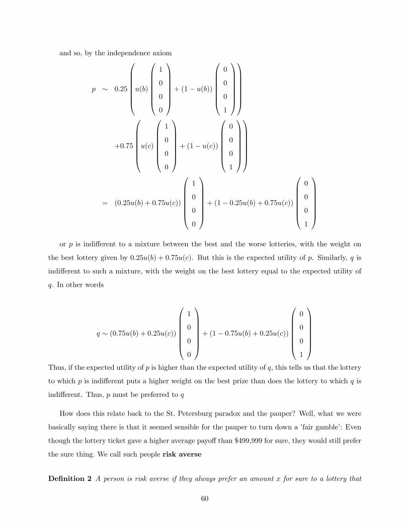
and so, by the independence axiom

∼ 025

⎛⎜⎜⎜⎜⎜⎜⎝()

⎛⎜⎜⎜⎜⎜⎜⎝1

0

0

0

⎞⎟⎟⎟⎟⎟⎟⎠+ (1− ())

⎛⎜⎜⎜⎜⎜⎜⎝0

0

0

1

⎞⎟⎟⎟⎟⎟⎟⎠

⎞⎟⎟⎟⎟⎟⎟⎠

+075

⎛⎜⎜⎜⎜⎜⎜⎝()

⎛⎜⎜⎜⎜⎜⎜⎝1

0

0

0

⎞⎟⎟⎟⎟⎟⎟⎠+ (1− ())

⎛⎜⎜⎜⎜⎜⎜⎝0

0

0

1

⎞⎟⎟⎟⎟⎟⎟⎠

⎞⎟⎟⎟⎟⎟⎟⎠

= (025() + 075())

⎛⎜⎜⎜⎜⎜⎜⎝1

0

0

0

⎞⎟⎟⎟⎟⎟⎟⎠+ (1− 025() + 075())⎛⎜⎜⎜⎜⎜⎜⎝0

0

0

1

⎞⎟⎟⎟⎟⎟⎟⎠or is indifferent to a mixture between the best and the worse lotteries, with the weight on

the best lottery given by 025() + 075(). But this is the expected utility of . Similarly, is

indifferent to such a mixture, with the weight on the best lottery equal to the expected utility of

. In other words

∼ (075() + 025())

⎛⎜⎜⎜⎜⎜⎜⎝1

0

0

0

⎞⎟⎟⎟⎟⎟⎟⎠+ (1− 075() + 025())⎛⎜⎜⎜⎜⎜⎜⎝0

0

0

1

⎞⎟⎟⎟⎟⎟⎟⎠Thus, if the expected utility of is higher than the expected utility of , this tells us that the lottery

to which is indifferent puts a higher weight on the best prize than does the lottery to which is

indifferent. Thus, must be preferred to

How does this relate back to the St. Petersburg paradox and the pauper? Well, what we were

basically saying there is that it seemed sensible for the pauper to turn down a ’fair gamble’: Even

though the lottery ticket gave a higher average payoff than $499,999 for sure, they would still prefer

the sure thing. We call such people risk averse

Definition 2 A person is risk averse if they always prefer an amount for sure to a lottery that

60

has an expected value of

Are people risk averse? In general, yes, but not always (after all, people do by lottery tickets!)

Bernoulli’s explanation was that risk aversion comes about if people have decreasing marginal

utility of wealth. This may seem to be a bit of a mysterious statement. How are these two

linked? Well, it turns out they they do indeed imply each other if the person is an expected utility

maximizer. We will show this graphically now, and you will show it formally for homework.

In order to answer this question, we first need to remember what a utility function that exhibits

decreasing marginal utility looks like. The answer should come quickly if you think about the work

we have done on production: such a utility function will be concave, as shown in figure 36. Figure

37 shows how to calculate the expected utility of a gamble that gives an amount with probability

0.5 and with utility 0.5 - you can read it off the line segment that connects the two. However,

for a concave function, this will always be below the utility of getting 05 + 05 for sure. Thus,

an individual who exhibits decreasing marginal utility will have a concave utility function and so

exhibit risk aversion.

61