Consumer Preference Analysis on - U of T · Consumer Preference Analysis on Cell Phone Plan Application ChoongHee Yun A thesis is submitted in partial fulfillment of the requirements

Consumer Preference Analysis on

Cell Phone Plan Application

ChoongHee Yun

A thesis is submitted in partial fulfillment

of the requirements for the degree of

BACHELOR OF APPLIED SCIENCE

Supervisor: Chi-Guhn Lee

Department of Mechanical and Industrial Engineering

University of Toronto

March, 2007

ABSTRACT. This report demonstrates the rate of importance of each feature on consumer

preference towards a particular cell phone plan. The data was collected by distributing

surveys to specific participants who are familiar with cell phones. Three parts of the survey

used distinct design techniques to create questions in three different forms. Using the data

collected from survey, in-depth statistical analysis was performed on each part to observe

the consumer preference and utility on the cell phone plan features in consideration.

Furthermore, three sets of results were compared to observe the consistency or variation in

consumer behavior due to change in the form of questions being asked.

- 1 -

1. INTRODUCTION Cell phone usage has become necessity for majority of the population; therefore, selling

cell phones and service plans takes majority of market share for most of the companies in

telecommunication industry. As a result, competition in selling cell phone plans has been

greatly intensified during past few years. To attract customers, it is important to know the

consumer’s preference towards cell phone plans being offered. In this project, surveys will

be designed with an effort to resemble the real-life situation as closely as possible by

considering all the factors affecting the contract process. Afterwards, the data collected

from this survey will be used to evaluate the consumer behavior. During the analysis phase,

there are several goals to be achieved.

The first purpose of this research is to observe the effect of each feature on consumer’s

preference towards a particular cell phone plan. Using the ratings on hypothetical cell

phone plans in the survey provided by respondents, the purpose was to detect change in

choice behavior relative to change in the level of certain features.

Furthermore, additional analyses were performed to compare the consistency and

differences between preferred cell phone plans obtained from the survey constructed, and to

decide which survey design method is most appropriate for this experiment. The survey

was designed using three different techniques. The data collected from these surveys was

observed to figure out whether different survey design techniques had any effect on

respondent’s decision.

Another subject of interest in this research is to figure out a way to include some of the

features which do not have any discrete quantitative scale of values to represent the levels

within the attribute. Such features are related to the additional services involved with

- 2 -

various cell phone plans. The key issue is to observe the effect of these features to change

in customers’ behavior.

In the Literature Review Section, the underlying concepts and theories behind my research

will be described. Section 3 and section 4 explains how the survey was designed and some

troubles encountered from Data Collection process, respectively. Section 5 details the

analysis performed on the data collected, followed by the formulation of general utility

model in Section 6. The results obtained will be summarized in Section 7.

- 3 -

2. LITERATURE REVIEW

2.1. Design of Experiments

Experiments are usually performed for discovery and testing of a particular subject of

interest. Montgomery (2005) emphasizes that experimental design is an important tool for

product design and development as well as process development and improvement. In the

design of experiments, the features are represented as factors, and the strength of these

features are represented as levels within each levels. For the purposes of this research, it is

assumed that the factors are fixed and the designs are completely randomized.

The effect of a factor is described as the change in decision influenced by a change in the

levels of the factor. This is known as the Main Effect. In addition, Interaction Effect

between factors is observed if change in levels of some other factors will result in the

variation of the main effect of a particular factor in consideration.

2.1.1. 2k Factorial Design

When designing experiments, dividing a factor into two levels is known as the most

common representation of the attribute. It is also particularly useful when there are many

factors to be investigated. In fact, Montgomery (2005) argues that two-level factorial

designs should be the cornerstone of industrial experimentation for product and process

development and improvement.

One of the very crucial assumptions made for 2-level attributes is that the response is

approximately linear over the range of the attribute levels selected. Since the observation in

the experiment is focused on the relative importance of each attribute, the absolute values

chosen for the levels of the factor does not have major effect on the result. For quantitative

- 4 -

attributes, each level is represented by values consistent with real-life scenario. For

qualitative attributes which cannot be expressed with discrete numbers, the levels are

simply represented by low / high, or -1 / 1.

2.1.2. 3k Factorial Design

It is possible to represent an attribute in 3-level when the variation in results due to a

change in the attribute is likely to be non-linear. Since 2k factorial design states that the

relationship between the range of two levels is assumed to be linear, 3-level has to be

employed for the attributes which has quadratic relationship between the selected range for

the levels. However, Montgomery (2005) strongly argues that 3k factorial design is not

efficient and unnecessarily complex. Therefore, in the mixed level factorial design, where

the mix of 2-level and 3-level factors are considered together, 3-level factors are

represented by combination of two 2-level factors, thus converting the entire problem into

2k factorial design. The low 3-level is reproduced as a combination of two low 2-levels,

medium 3-level as a combination of one low and one high 2-level, and high 3-level as a two

high 2-levels.

2.1.3. Fractional Factorial Design

For types of experiments involving multiple factors, factorial design is known as the most

efficient technique to be employed (Montgomery 2005). Factorial design investigates all

possible combinations of the levels of the factors. The greatest weakness of full factorial

design is that this method becomes infeasible as number of factors become large. Since

each factor is divided into two or more levels, the number of possible combinations of

factors increases exponentially for every time an additional factor is added.

- 5 -

To resolve this problem, fractional factorial design should be used. Most of the experiments

conducted tend to be large; consequently, fractional factorial design is one of the most

widely used design technique (Montgomery 2005). Montgomery (2005) also states that

fractional factorials are often used in “screening experiment” – experiments where the

objective is to observe which factors have large effect.

In the fractional factorial design, high-order interactions are eliminated due to aliases.

“Alias” is the term used to indicate certain main effects or interaction effects identical

factorial combinations. When there are no aliases between main effects but they are aliased

with two-factor interaction effects, this is called “Resolution III Design”. Therefore,

fractional factorial design is applied under the assumption that certain high-order

interactions are negligible.

2.2. Economic Valuations

Economic valuation is the interpretation of the value of certain goods or services based on

the preference of the individual consumers, rather than the statistics in the market place.

Bateman et al.(2002) summarizes economic valuation as the assignment of money values to

non-marketed assets, goods and services, where the money values have a particular and

precise meaning. The goods or services are considered to have positive economic value if

they can contribute to human wellbeing, which is judged by satisfaction on the people’s

preference. One of the ways in which the consumer preference can be evaluated is by

acquiring the maximum amount that may be contributed by the individual to equalize a

utility change. This is known as consumer’s “Willingness to Pay”.

- 6 -

2.2.1. Consumer Preference

The two methodologies for quantifying the consumer preference towards goods and

services are revealed preference method and stated preference method. Revealed preference

technique determines the consumer preference by analyzing the real market behavior,

which represents the actual transactions done by consumers. In comparison, stated

preference technique assesses the consumer preference by directly asking people in the

hypothetically constructed scenario, such as survey. The table below lists and contrasts

some of the characteristics of revealed preference techniques and stated preference

technique.

Revealed Preference Data Stated Preference Data Based on actual market behaviour Based on hypothetical scenarios Attribute measurement error Attribute framing error Limited attribute range Extended attribute range Attributes correlated Attributes uncorrelated by design Hard to measure intangibles Intangibles can be incorporated Cannot directly predict response to new alternative

Can elicit preferences for new alternatives

Preference indicator is choice Preference indicators can be rank, rating, or choice intention

Cognitively congruent with market demand behaviour

May be cognitively non-congruent

<Table 1: Characteristics of revealed vs. stated preference Data (2002)> Stated preference technique can be partitioned to two methods, contingent valuation and

choice modeling. For contingent valuation, the respondents are directly asked for dollar

values of certain goods or services. Choice modeling, also know as conjoint analysis, is

described in the following section.

2.2.2. Conjoint Analysis

Conjoint analysis, also known as choice modeling, is a technique used mainly in designing

surveys, to determine the respondents’ preferences for products or services. The key

- 7 -

characteristic of conjoint analysis is that respondents evaluate product profiles composed of

multiple conjoined attributes or features (Orme, 2002). Conjoint analysis provides

information on individual and synergetic effects of the attributes. Therefore, conjoint

analysis provides the insight on consumer preference by providing the rate of importance of

each attribute. Asking respondents to indicate choices for realistic sets of alternatives most

closely resembles the market problem (McFadden, 1986). By creating hypothetical

products and observing people’s behavior from respondents’ data, accurate information on

consumer’s preferences can be analyzed.

2.3. Survey Design Techniques

In this project, three different survey design techniques were used, thus asking questions in

three different forms in the survey. These three design methods include Self-Explicated

Design, Full Profile Design and Choice-Based Conjoint Design.

2.3.1. Self–Explicated

The self-explicated design is considered the most simplistic survey design technique. For

self-explicated design, the evaluation is focused on the effect of individual attributes, rather

than comparing actual profiles created by bundle of features. The general question being

asked for each of the attribute is: “With everything else remaining constant, how important

is the change in level of this particular attribute in the preference towards a particular

profile?”. Consequently, this method is prone to error if there are any interactions between

features. This method has the advantage of reducing information overload for the cases

where many attributes are considered. On the other hand, it is limited to individual ranking,

- 8 -

which leads to biased responses. The survey results will provide information on individual

respondent’s preference for each of the attribute. Because direct evaluation draws attention

to attribute levels, it tends to overweight attributes that might otherwise be unimportant in a

competitive context (Huber, 1997).

2.3.2. Full Profile

Full profile design technique is known to be most useful for measuring around six attributes.

This method asks respondents to rate each profile separately, where an individual profile

contains certain combination of attributes bundled together. The hypothetical profiles

generated from factorial design closely reflects the products or services in real life, making

the consumer preference obtained from the survey a fairly accurate representation of real

interaction situation. Since respondents are evaluating profiles consisting of combinations

of different levels of attributes altogether, the less important attributes are naturally ignored

when rating a certain profile. In full profile design, the purchase likelihood of every profile

is asked separately, respondents’ decision will strictly depend on the quality of attributes

within the profile. The focus of the decision is within alternative so that the explicit

comparisons between numbers of option are rare (Huber, 1997).

When the profiles are generated from full factorial design, which considers every possible

combination of all the attributes, increase in number of attributes results in an exponential

increase in number of profile. To resolve this problem, fractional factorial design can be

employed to reduce the number of profiles.

- 9 -

2.3.3. Choice-Based Conjoint

In choice-based conjoint method, the respondents are given with set of profiles to choose

from in each choice set. The procedure for generating hypothetical profiles is identical to

full profile method, by using factorial design. Within each choice set, there is also a “No

buy” option as one of the selections. Similar to full profile, the choice made by respondents

will mainly depend on most preferred attributes. Comparison between important attribute

will be the factor affecting preferred choice the most.

The set of plans in each of the choice set are produced using a “mix and match” approach

on the profiles produced from design of experiments, described by Louviere(1988). This

algorithm shuffles certain attributes from original combination of plans found by factorial

design of experiment, which will produce another set consisting of different combinations

of plans.

There are some weaknesses regarding choice-based conjoint technique. When there are

many choices for respondents to consider, with each choice set containing multiple

attributes, respondents’ decision tend to skew towards the choices that simply have specific

attributes they prefer.

2.4. Statistical Analysis

The two key analysis techniques used in this research are Analysis of variance and

regression analysis. These analyses are performed on a set of data to observe variations and

correlations between data sets. The subsections below describe these two analyses

techniques extensively.

- 10 -

2.4.1. Analysis of Variance (ANOVA)

The analysis of variance for a model assumes that the observations are normally and

independently distributed, with the same variance in each treatment or factor level (Hines,

Montgomery, Goldsman, Borror, 2003). These assumptions can be validated by graphing

normal probability plots and residual plots.

The analysis of variance is performed on the data to observe the main effects of individual

attributes as well as any significant interaction effects of bundles of attributes. Although it

is possible to have any combination of factors to examine the interactions, interaction

effects are only considered up to two factors for the purposes of this research. The

ANOVA table for 2-way interaction is shown below, with the detailed computations for

each category.

Source of Variation

Sum of Squares Degrees of Freedom

Mean Square F0

A Treatments ∑

=

−=a

i

iA abn

ybnySS

1

2...

2..

1−a 1−

=aSSMS A

A E

A

MSMSF =0

B Treatments ∑

=

−=b

i

jB abn

yany

SS1

2...

2..

1−b 1−

=bSSMS B

B E

B

MSMSF =0

Interaction ∑∑= =

−−−=a

iBA

b

jijAB SSSS

abnyy

nSS

1

2...

1

2.

1

)1)(1( −− ba )1)(1( −−

=ba

SSMS ABAB

E

AB

MSMSF =0

Error BAABTE SSSSSSSSSS −−−= )1( −nab

)1( −=

nabSSMS E

E

Total ∑∑∑= = =

−=a

i

b

j

n

kijkT abn

yySS1 1 1

2...2

1−abn

<Table 2: The ANOVA Table for the Two-Factor Factorial>

Although the ANOVA table above only illustrates the case where there are two factors to

consider, this concept is the basis for analyzing the main and two-way interaction of

features in this research.

- 11 -

The F-test is a parametric test which can be used only if the normality assumption on the

data is validated. The F ratio in the ANOVA table can be interpreted as the comparison

between the actual variation of the group averages and the theoretically expected variation.

Therefore, if the F ratio value is high, this is an indication that the particular attribute has

significant effect.

The P-value is interpreted as a measurement identifying the data consistency, assuming the

null hypothesis is true. The null hypothesis presumes that the treatments will not have any

effect. In general, smaller p-value is an indication that there exists a great inconsistency

between the actual data and the hypothesis. Applying this underlying concept to current

research, if the P-value extracted from ANOVA of each factor is small, it means that

feature has a very strong effect.

2.4.2. Regression Analysis

In general, regression analysis is a statistical technique for modeling and investigating the

relationship between two or more variables (Hines, Montgomery, Goldsman, Borror, 2003).

The regression equation exemplifies the relationship between dependent and independent

variables. Dependent variables are called response variables, and independent variables are

called regressor variables. This form of equation can be fitted into a set of data to create a

regression model.

The adequacy of regression model has to be measured when fitting a regression model.

Estimation of model parameters requires the assumption that the errors are uncorrelated

random variables, which are normally distributes with mean zero and constant variance

(Hines, Montgomery, Goldsman, Borror, 2003). These assumptions can be confirmed with

normal probability plots and residual plots.

- 12 -

It is very important to validate the regression model. One of the techniques used to measure

the adequacy of a multiple regression model is the “coefficient of multiple determinant, R2”.

This coefficient is defined as:

Coefficient of Multiple Determinant Non-adjusted Adjusted

T

E

SSSSR −=12

)1(

)(12

−

−−=

nSS

pnSS

RT

E

adj

<Table 3: Non-adjusted / Adjusted coefficient of multiple determinant>

R2 is a measure of the amount of reduction in the variability of response variable obtained

by using the regressor variable (Hines, Montgomery, Goldsman, Borror, 2003). According

the equations given in above table, non-adjusted R2 value cannot necessarily guarantee a

better fit regression because this value will increase with the number of regressor variables.

On the other hand, the value of adjusted R2 will only increase if the mean square for error is

reduced, which is presented as numerator in the equation.

2.5. Utility Theory

Utility can be defined as the measure of consumer’s satisfaction towards certain goods or

services. Weitzman (1965) states that each person is assumed to possess a subjective

preference pattern among alternative situations, and a utility function is any function that

arithmetizes the relation of preference among the situations. When working with stated

preference data, it is critical to recognize that the analysis should be done concentrating on

the relative scale of utility values. When there are multi-attributes to consider, information

about the consumer preference of certain combination of attributes can be studied to figure

out the relative importance of each attribute.

- 13 -

2.5.1. Multi-Attribute Utility Function

Multi-attribute utility models are tools used to evaluate and compare the decision making

process towards a set of alternatives, where each alternative consists of bundle of attributes

combined together. By creating the generalized function representing the utility, it is

possible to assign scores to available choices in the decision situation if the set of

alternatives can be identified. It is essential to note that when there are many number of

features involved in a profile, the decision making process on one’s utility will primarily

depend on set of factors that are of greatest importance. Schäfer (2002) states that due to

the high number of attributes, the user cannot be queried about each value function and

each attribute.

If there are n components of attributes x to consider in the utility model, the additive utility

function is expressed as:

( )nxxxxx ..,,.........,, 321=

∑=

=n

iii xUpEU

1)( ;

Where pi = preference weight of attribute i EU = expected utility <Figure 1: Utility Model expression>

The outcomes will be expected utilities of set of profile, mathematically written in terms of

the utility of individual attributes involved. In this research, the information regarding

expected utilities is obtained from the data, with the goal of determining appropriate

preference weight of each feature.

- 14 -

3. SURVEY DESIGN & DEVELOPMENT

3.1. Selection of Attributes

The first step to creating a survey is to decide on which features to include in each profile

representing a one complete cell phone plan. Within each feature, there are two or three

distinct levels, which represent the strength or contribution of that particular feature in the

profile. The table below illustrates list of features which will be used to create cell phone

product lines.

Criteria Features Values Price Price of Plans 35, 50, 65 ($) Time Anytime 100, 350 (Minutes) Evening & Weekends 400, Unlimited (Minutes) Additional Features Voice Mail Included, Excluded Caller ID Included, Excluded Duration of Contract Length of Contract 1, 2, 3 (in years) Additional benefits/services Discount on Cell Phone 45, 75, 105 ($) Cash Value of Service 30, 45, 60 ($) <Table 4: Description of features> The selection of features and their levels to be included in the survey are carefully

considered to best reflect the real contract. This will make sure that the attributes included

in our product line will be useful in analysis. Moreover, since the valid survey respondents

are restricted to people who have used cell phone before, they will most likely be familiar

with the features.

In general, the major issues when signing a contract for a cell phone service would be the

cost associated, and the amount of minutes available for phone calls. Although it is more

preferable to have two levels within an attribute, three levels are used in the Price feature to

be more specific. The time criterion was divided into two attributes because this is how

companies normally offer their service.

- 15 -

There are many additional features such as text messaging, voice mail, caller ID, detailed

billing and more, which could be considered in cell phone service. However, it was proven

from previous thesis paper that many of these features do not have significant effect on

respondents’ decision. Since it is meaningless in this project to include such features, only

two of the additional features which are most likely to impact the respondents’ decision are

included.

The challenging part was to include additional services attached with the contract by

creating appropriate attributes to represent these service features. Although this feature is

not the actual component of a cell phone plan, it is a major part of the contracting process

that could greatly affect customers’ decision. In reality, additional service can be anything

which gives extra benefits to the customer. Therefore, there are countless possible ways for

a company to offer extra services. However, since the number of attributes cannot be very

large, this criterion is generalized into two features. This was done by quantitatively

representing additional services coming from forming a contract in terms of cash value. For

instance, cash value of additional service being $30 means all the services offered

combined worth approximately $30. In addition, discount on cell phone was added because

there is usually large discount on price of the phone itself if it was purchased with the

contract.

3.2. Generation of Cell Phone Plans

After having all the appropriate features, the next step was to bundle the features together to

create hypothetical cell phone plans that are going to be included in the survey. Since there

are four features with 3 levels and four features with 2 levels, this corresponds to set of

- 16 -

34*24=1296 feasible plans. The complexity with this process was that the number of

questions asked in the survey should be limited to approximately 15 questions to obtain

reliable data from the respondents. If too many questions are being asked in the survey, it is

very likely that the respondents’ will lose their concentration during the process.

The key importance in generating only limited number of hypothetical cell phone plans was

to have appropriate product lines which will ensure that all the required information in

analysis phase is gathered from the data collected by surveys. This process was done based

on the background theory of fractional factorial design. The table below lists all the factors

and their corresponding levels:

Factors Levels [A] (Voice Mail) High; Low [B] (Anytime) High; Low [C] (Caller ID) High; Low [D] (Evening & Weekends) High; Low [E] (Length of Contract) High; Med; Low [F] [G] (Price of Plan) High; Med; Low [H] [J] (Discount Cell Phone) High; Med; Low [K] [L] (Cash Value of Service) High; Med; Low [M] <Table 5: List of features and corresponding levels> The factors in Table 2 represent the features included in the hypothetical plans. Also, the

levels represent the values within each feature, where high level corresponds to higher

value. For factors with 3 levels, these are considered as combination of two 2-level factors.

As a result, there are twelve 2-level factors in total. Using fractional factorial design

technique, the 2III12-8 Design was implemented, which resulted in 16 plans to be evaluated.

Although this process eliminates the higher order interactions due to aliases, this research

- 17 -

does not require analysis of high-order interaction effects. The table below illustrates

Design of Experiment for 2III12-8 Design:

Basic Design Run A B C D E=ABC F=ABD G=ACD H=BCD J=ABCD K=AB L=AC M=AD 1 -1 -1 -1 -1 -1 -1 -1 -1 1 1 1 1 2 1 -1 -1 -1 1 1 1 -1 -1 -1 -1 -1 3 -1 1 -1 -1 1 1 -1 1 -1 -1 1 1 4 1 1 -1 -1 -1 -1 1 1 1 1 -1 -1 5 -1 -1 1 -1 1 -1 1 1 -1 1 -1 1 6 1 -1 1 -1 -1 1 -1 1 1 -1 1 -1 7 -1 1 1 -1 -1 1 1 -1 1 -1 -1 1 8 1 1 1 -1 1 -1 -1 -1 -1 1 1 -1 9 -1 -1 -1 1 -1 1 1 1 -1 1 1 -1 10 1 -1 -1 1 1 -1 -1 1 1 -1 -1 1 11 -1 1 -1 1 1 -1 1 -1 1 -1 1 -1 12 1 1 -1 1 -1 1 -1 -1 -1 1 -1 1 13 -1 -1 1 1 1 1 -1 -1 1 1 -1 -1 14 1 -1 1 1 -1 -1 1 -1 -1 -1 1 1 15 -1 1 1 1 -1 -1 -1 1 -1 -1 -1 -1 16 1 1 1 1 1 1 1 1 1 1 1 1 <Figure 2: Design of Experiment for 2III

12-8 Design> Each run in Table 3 represents a one complete cell phone plan which will be included in the

survey, which results in sixteen questions to be asked. For the 2-level factors, {-1}

corresponds to low level, and {1} corresponds to high level. As for the 3-level factors, {-1,

-1} combination corresponds to low level, {-1, 1} or {1, -1} combination corresponds to

medium level, and {1, 1} combination corresponds to high level.

3.3. Survey Construction

There are three parts in the first-round survey, which was designed using the three well-

known techniques described in the literature review. These techniques are Self-explicated

Design, Full Profile Design, and Choice Based Conjoint Design.

- 18 -

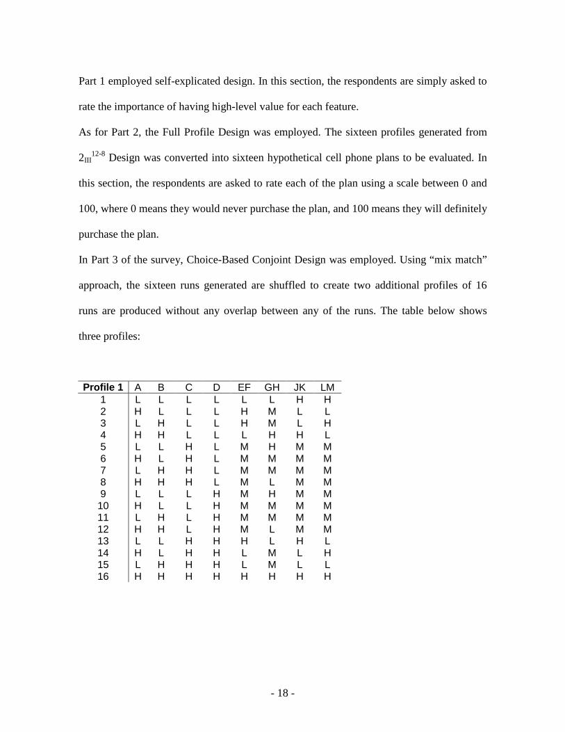
Part 1 employed self-explicated design. In this section, the respondents are simply asked to

rate the importance of having high-level value for each feature.

As for Part 2, the Full Profile Design was employed. The sixteen profiles generated from

2III12-8 Design was converted into sixteen hypothetical cell phone plans to be evaluated. In

this section, the respondents are asked to rate each of the plan using a scale between 0 and

100, where 0 means they would never purchase the plan, and 100 means they will definitely

purchase the plan.

In Part 3 of the survey, Choice-Based Conjoint Design was employed. Using “mix match”

approach, the sixteen runs generated are shuffled to create two additional profiles of 16

runs are produced without any overlap between any of the runs. The table below shows

three profiles:

Profile 1 A B C D EF GH JK LM 1 L L L L L L H H 2 H L L L H M L L 3 L H L L H M L H 4 H H L L L H H L 5 L L H L M H M M 6 H L H L M M M M 7 L H H L M M M M 8 H H H L M L M M 9 L L L H M H M M

10 H L L H M M M M 11 L H L H M M M M 12 H H L H M L M M 13 L L H H H L H L 14 H L H H L M L H 15 L H H H L M L L 16 H H H H H H H H

- 19 -

Profile 2 A B C D EF GH JK LM 1 H H H H M M L L 2 L H H H L H M M 3 H L H H L H M L 4 L L H H M L L M 5 H H L H H L H H 6 L H L H H H H H 7 H L L H H H H H 8 L L L H H M H H 9 H H H L H L H H

10 L H H L H H H H 11 H L H L H H H H 12 L L H L H M H H 13 H H L L L M L M 14 L H L L M H M L 15 H L L L M H M M 16 L L L L L L L L

Profile 3 A B C D EF GH JK LM

1 L L L L H H M M 2 H L L L M L H H 3 L H L L M L H M 4 H H L L H M M H 5 L L H L L M L L 6 H L H L L L L L 7 L H H L L L L L 8 H H H L L H L L 9 L L L H L M L L

10 H L L H L L L L 11 L H L H L L L L 12 H H L H L H L L 13 L L H H M H M H 14 H L H H H L L M 15 L H H H H L L H 16 H H H H M M M M

<Figure 3: Three profile combinations generated from Mix-and-Match approach> Plans from each profile were picked one at a time to for each choice set to be included in

the survey. Also, for each choice set, a fourth choice, “Do not purchase this Plan”, was

included.

The complete survey is attached in the Appendix 1.

- 20 -

4. DATA COLLECTION

The set of data used to perform various statistical analyses were collected by distributing

the survey (Appendix A) that has been constructed. The three distinct parts were put

together into one survey and respondents were required to answer every single question the

survey. There were some restrictions on the respondents who are eligible to participate in

this research. The qualified respondents should satisfy the following criteria:

1. Currently a resident of Ontario

2. Currently a university/college student

3. Presently using cell phone, have used it before, or plan to purchase one within the

next six month

The respondents were restricted to Ontario residents to ensure that all of them will

understand the Canadian currency. Also, since other regions in Canada might have a price

standard that is inconsistent with Ontario, restricting the respondents to people living in

Ontario will guarantee that they are paying compatible price for their cell phone plans.

Moreover, respondents were narrowed down to university students to make sure that all of

the respondents would have similar standards on the money value. For instance, $20 to 10

years old would have different value than to 20 years old. Lastly, respondents were

required have some experience with cell phone usage and therefore familiar with billing

system of cell phone plans.

All these restrictions were applied to improve the accuracy of data and reduce outliers.

However, since the survey was fairly long, there were some problematic data which had to

be discarded for more accurate analysis results. Since the sample size was not very large,

even one biased data set could have significant effect on the result. A total of 32

- 21 -

respondents completed the survey. However, nine of them were excluded from the analysis

because they interpreted the survey questions differently. Although 23 data sets are merely

enough to represent the preference of entire population, the analyses were done with this

data due to time limitations.

- 22 -

5. DATA ANALYSIS

With 23 data sets collected from the survey, various analyses were performed on each part

distinctly to evaluate and compare the results. In the following subsections, the results

obtained from the analysis methods applied to data sets for self-explicated, full profile, and

choice-based conjoint will be explained.

5.1. Self–Explicated

From the data set collected for self-explicated survey, preference ratings and part-worth

utilities were computed to evaluate the importance of each attribute.

5.1.1. Preference Rating

As mentioned above, respondents were asked to rate each attribute between scales of one to

four, with one being least important and four being most important. The table below lists

the preference rating of each attribute.

Attribute Average Importance

Preference Ratings

Price of Plans 3.66 0.91 Anytime 2.69 0.67 Evening & Weekends 2.81 0.70 Voice Mail 2.06 0.52 Caller ID 3.19 0.80 Length of Contract 2.72 0.68 Discount on Cell Phone 3.06 0.77 Cash value of Service 2.31 0.58

<Table 6: Preference rating of each attribute from Self-Explicated Design>

According to the result, people’s preferences toward the attributes are as follows: 1) Price of Plan 2) Caller ID 3) Discount on Cell Phone 4) Evening and Weekend Minutes 5) Length of Contract

- 23 -

6) Anytime Minutes 7) Cash Value of Service 8) Voice Mail

From the preference ratings, it is easy to notice that price of plan is the dominating feature

that consumers consider when choosing a cell phone plan. This was followed by discount

on the cell phone price, indicating that most consumers’ primary concern is the issue

involving cost. One unexpected factor that was considered highly important to many of the

respondents was the caller ID feature.

5.1.2. Part-Worth Utility

The importance ratings obtained from respondents can be directly applied to finding the

part-worth utilities of each feature. As mentioned before, the absolute scale of utility values

is meaningless in the stated preference data, which can be set arbitrarily. Therefore, the

focus should be on the relative importance of the attribute compared to the other attributes.

In this research, the part-worth utility of each attribute for individual respondent was

determined by dividing the importance rating by two. A spreadsheet all the part-worth

utility is attached in Appendix 2.

The part-worth utilities can be used to more precisely distinguish the consumer preference

between attributes. From the preference ratings in table 6, attributes such as length of

contract and anytime minutes, or discount on cell phone and caller ID have very similar

preference ratings. By comparing the utility of each individual respondent, the factor that is

preferred by more people can be determined, which can be resolved as attribute with higher

importance. The table below illustrates the pairwise comparison between two attributes

stated previously.

- 24 -

Attributes Utility Dominance (Counts) Length of Contract 10 Anytime Minutes 8 Discount on Cell Phone 8 Caller ID 6

<Table 7: Part-worth Utility Pairwise Comparison>

From the pairwise comparison of part-worth utilities, more respondents picked length of

contract and discount on cell phone to have greater influence than anytime minutes and

caller ID, respectively.

5.2. Full Profile

From the data set collected for full profile survey, analysis of variance and regression

analysis are performed to evaluate the importance of individual attributes as well as any

notable interactions between attributes. Minitab software was used for both statistical

analyses.

Before the analyses are done, the normality and independence of data set was confirmed.

The figures below are normal probability plot of residuals and plot of residuals versus fitted

value.

<Figure 4: Normal Probability plots & Residual vs. Fitted value>

7060504030

8

6

4

2

0

-2

-4

-6

-8

Fitted Value

Res

idua

l

Residuals Versus the Fitted Values(response is Avg. Rat)

86420-2-4-6-8

2

1

0

-1

-2

Nor

mal

Sco

re

Residual

Normal Probability Plot of the Residuals(response is Avg. Rat)

- 25 -

5.2.1. Analysis of Variance (ANOVA)

From the figure 4 above, the data points closely resembling straight line on “normal

probability plot of the residuals” supports the normality assumption. Also, randomly

distributed data points without any noticeable pattern on “residuals versus fitted values

plot” the data are independently distributed.

The analysis of variance was conducted with the features as independent variable and

responses as dependent variable. The combination of attributes for each hypothetical plan

and their corresponding purchase likelihood is shown in Appendix C1. The table below

shows the results found from ANOVA.

Source of Variation DF SS MS F P Voice Mail 1 4 4 0.02 0.901 Anytime 1 171 171 0.79 0.393 Caller ID 1 384 384 1.86 0.194 Evening & Weekends 1 334 334 1.6 0.227 Length of Contract 2 81 41 0.17 0.849 Price of Plan 2 2045.9 1022.9 10.89 0.002 Discount on Cell Phone 2 81 41 0.17 0.849 Cash Value of Service 2 13 6 0.03 0.975 Total 15

<Table 8: ANOVA Table for individual attributes> The ANOVA table results indicate that price of plan had the greatest effect on

respondent’s purchase likelihood. In addition, evening & weekend minutes and caller ID

were also influential on respondent’s decision. Anytime minutes had a minor effect on

respondent’s preference towards a given plan. However, rest of the attributes had almost no

effect on the purchase likelihood of cell phone plans. The graphical representation of this

analysis result is illustrated by main effect plot, attached in Appendix C2. This result

reveals consumer behavior of basing the purchase likelihood by simply considering the

level of attribute which are important in the decision making process.

- 26 -

There was only few interaction effects observed between the combinations of two attributes.

With a compactly compressed 2III12-8 fractional factorial design, the number of possible

two-way interaction effects that could be checked was only three. Moreover, with each cell

hone plan having eight attributes to consider, the respondents’ preference heavily depended

on the level of attributes with high importance. According to the F-ratio found from one-

way ANOVA, most of the respondents selected the cell phone plan with cheapest price.

Appendix C3 shows two interaction plots. First graph is the interaction plot between price

and caller ID, and second one is between anytime and evening & weekend minutes. In

general, the two lines represent the behavior of attribute on x-axis as the interacting

attribute’s level was changed from low to high. Although two lines in the graph do not

cross, there is still and indication of weak interaction between these attributes because the

slopes of the lines differ.

5.2.2. Regression Analysis

Prior to fitting a regression model, the normality and independence of errors have to be

checked. Similar to ANOVA, these assumptions can be validated by observing “normal

probability plot of the residuals” and “residuals versus fitted values plot”, shown in the

Figure 4 above. The data points closely resembling straight line on normal probability plot

supports the assumption that errors are normally distributed. In addition, randomly

distributed data points without any noticeable pattern on residual plots verify that the errors

are independently distributed, with no correlation.

The regression analysis was conducted to determine the regression model coefficients that

best fits the data set. Similar to the results analysis of variance, regression analysis with

data set for full profile design revealed that there are no significant interactions between

- 27 -

any two attributes; therefore, regression was conducted only with the individual features.

The regression model had a R2 value of 90% and adjusted R2 value of 77%, proving that

this regression model is a good fit. The table below illustrates coefficients found by fitting a

regression model.

Predictor Coef. Factor Levels Factor Coef. Constant 173.4 - 173.4 Voice Mail 0.967 1 0.967 Anytime 0.02613 350 9.1455 Caller ID 9.793 1 9.793 Eve&Weekend 0.00000915 999999 9.14999085 Contract -21.43 2 -42.86 Price -0.8857 50 -44.285 Discount 0.713 75 53.475 Service 0.0058 45 0.261

<Table 9: Regression coefficients for Full Profile Design>

The coefficients cannot be directly compared to diagnose the importance of each feature to

the respondents because for features such as price of plan or discount on cell phone, the

actual values are used to represent each level. For instance, instead of scaling the values

and using 0 as low level and 1 as high level, the levels for price feature was 30 dollars, 50

dollars and 65 dollars. To convert everything to equalized scale, factor coefficients are

computed by multiplying the regression coefficient for each attribute by its corresponding

level values.

Positive coefficients for voice mail, anytime, discount on cell phone, caller ID, cash value

of service and evening & weekend minutes indicate that increase in the level of these

features increase the value of the plans. In comparison, negative coefficients in front of

Contract and Price indicate consumers prefer shorter contract and lower price. Moreover,

the attributes strongly affecting the respondents’ preference have the high absolute factor

coefficients, as shown in table 9.

- 28 -

The complete analysis result is attached in Appendix D.

5.3. Choice-Based Conjoint

From the data set collected for choice-based conjoint questions, the chosen proportion of

each level of individual attributes was computed and regression analysis is performed to

evaluate the importance of individual attributes. Minitab software was used.

5.3.1. Proportions

The proportion for each attribute was computed by finding the ratio between the number of

times it was shown on the survey as part of a hypothetical plan and the number of times in

which the plan containing this particular attribute was chosen by the respondents. To take

into account the selection of “No Buy” option, the overall percentage of no buy option

chosen was calculated.

As a result of varying number of “No Buy” option selected for each choice set, the ratios do

not add up to one. Although the proportions can be easily rescaled by incrementing the

percentage of no buy option chosen, it is not necessary because the purpose of this research

is to observe relative importance. The table below lists the proportions of each level of

individual attributes.

- 29 -

Features Levels Proportions Anytime 100 0.208 350 0.2595 Evening & Weekend 400 0.2064 Unlimited 0.2614 Caller ID Yes 0.2973 No 0.1705 Voice Mail Yes 0.2519 No 0.2159 Contract Length 1 0.2415 2 0.2415 3 0.219 Discount on Cell Phone 50 0.2699 75 0.1307 105 0.3011 Cash Value of Service 30 0.2216 45 0.287 60 0.2074 Price of Plan 30 0.61 50 0.0597 65 0.0284 No Buy 0.3027

<Table 10: Proportion of each attribute chosen from choice-based questions> In general, the proportions show that respondents prefer longer minutes, more additional

features, and more discount services. The 30 dollar price of plan has the highest ratio of

61%, indicating that low price is the dominating factor when the respondents are deciding

on a cell phone plan.

- 30 -

6. CONSUMER UTILITY MODEL

Based on the stated preference data obtained from both full profile questions and choice-

based conjoint questions, general utility models were formulated to further analyze the

importance of each attribute as well as the consistency between two different survey design

techniques.

6.1. Overview

The consumer utility model serves as a generalized representation of consumer utility

towards a particular cell phone plan. The goal of formulating this model is to determine the

coefficients which would reflect the weighting on people’s preference of individual

attribute.

The values initially set as the levels of each attribute were directly implemented to the

formulation as the utility values of each level of attributes. This is valid since the focus of

analysis is on the relative importance, which means that the numbers themselves does not

contain any significance to the result.

Each attribute is assigned as one decision variable, under the assumption that the consumer

behavior between the low level and high level range is linear. However, the “Price of Plan”

feature is partitioned to two decision variables, assuming that consumer behavior for this

attribute is pairwise linear, as this pattern was shown in the main effects plot. The variables

involved with the formulation are defined in Appendix E1.

- 31 -

6.2. Utility Model Formulation

The objective of this formulation is to minimize the inconsistency on the rankings of

consumer utility. Since the rankings of utility for the cell phone plans was decided based on

the data collected from 23 people, and there are twenty to thirty hypothetical plans to

consider, there is a chance that the coefficients satisfying every single utility ranking might

not exist. The purpose is to find the solution that best satisfies as many utility rankings as

possible. In the following sub-sections, details about how the model was formulated and the

logic behind each constraint will be described.

6.2.1. Utility Model – Full Profile

The general formulation for determining the coefficients in the utility model is shown

below.

Objective:

Minimize ∑=

15

1iiS Ii∈∀

Constraints: - Consumer Utility Rank Constraints

kATUATi+ kEWUEWi+ kVMUVMi+ kCIUCIi+ kCLUCLi+ kDCUDCi+ kCVUCVi+ k1PU1Pi+ k2PU2Pi+ Si >= kATUATj+ kEWUEWj+ kVMUVMj+ kCIUCIj+ kCLUCLj+ kDCUDCj+ kCVUCVj+ k1PU1Pj+ k2PU2Pj+ Sj

Ii∈∀ & Jj∈ - Coefficient Range Constraints

-100 <= k <= 100 for each k - Positive Slack Constraint

Si >= 0 Ii∈∀ - Min/Max Utility Constraints

0 <= kATUATx+kEWUEWx+kVMUVMx+kCIUCIx

+kCLUCLx+kDCUDCx+kCVUCVx+k1PU1Px+k2PU2Px <= 100 Xx∈∀

<Figure 5: Utility Model Formulation for Full Profile>

- 32 -

In the Constraints given above, set {I} represents the set of plans on greater than side, set

{J} represents the set of plans on less than side, and set {X} represents the set with all the

cell phone plans included in full Profile Questions. Since there are 16 hypothetical cell

phone plan involved in full profile design, 15 utility ranking constraints for set {I} and set

{J} are specified as follows.

i j (Plan 6) >= (Plan 16) (Plan 8) >= (Plan 12) (Plan 16) >= (Plan 10)

(Plan 12) >= (Plan 13) (Plan 10) >= (Plan 9) (Plan 13) >= (Plan 15) (Plan 9) >= (Plan 4) (Plan 15) >= (Plan 14) (Plan 4) >= (Plan 3) (Plan 14) >= (Plan 1) (Plan 3) >= (Plan 5) (Plan 1) >= (Plan 7) (Plan 5) >= (Plan2) (Plan 7) >= (Plan 11)

(Plan 11) >= (Plan 6) <Table 11: Utility Rank for Full Profile Data> The ranking of hypothetical plans was derived from the preference score of respondents

obtained from the survey. The consumer utility rank constraints specify the plans having

higher or lower utility than other plans, as illustrated in table 11. The numerical values used

to represent the utilities for attributes in each of 16 plans are listed in Appendix E2.

Coefficient range constraints are included to set lower and upper bounds on the possible

values of each coefficient. Positive slack constraints are included to ensure that no slacks

become negative during the minimizing process. Lastly, min/max utility constraints would

restrict the utility for all plans to range between 0 and 100.

6.2.2. Utility Model – Choice Based Conjoint

The basic structure of utility model formulation for the choice-based conjoint is very

similar to the full profile case, as shown in Figure 6.

- 33 -

Objective:

Minimize ∑=

32

1iiS Ii∈∀

Constraints: - Consumer Utility Rank Constraints

kATUATi+ kEWUEWi+ kVMUVMi+ kCIUCIi+ kCLUCLi+ kDCUDCi+ kCVUCVi+ k1PU1Pi+ k2PU2Pi+ Si >= kATUATj+ kEWUEWj+ kVMUVMj+ kCIUCIj+ kCLUCLj+ kDCUDCj+ kCVUCVj+ k1PU1Pj+ k2PU2Pj+ Sj

Ii∈∀ & Jj∈ - Coefficient Range Constraints

-100 <= k <= 100 for each k - Positive Slack Constraint

Si >= 0 Ii∈∀ - Min/Max Utility Constraints

0 <= kATUATx+kEWUEWx+kVMUVMx+kCIUCIx

+kCLUCLx+kDCUDCx+kCVUCVx+k1PU1Px+k2PU2Px <= 100 Xx∈∀ <Figure 6: Utility Model Formulation for Choice-Based Conjoint> Since the set of hypothetical cell phone plans included in choice-based conjoint, set {X} in

this formulation consists of 48 cell phone plans, which are listed in Appendix E3 with the

corresponding numerical utility values for the attributes in each plan. Regarding the

consumer utility rank constraints, the cell phone plans in set {I} and set {J} are listed in the

table below.

i j (Plan 9.2) >= (Plan 9.3) (Plan 1.1) >= (Plan 1.2) (Plan 9.3) >= (Plan 9.1) (Plan 1.2) >= (Plan 1.3) (Plan 10.3) >= (Plan 10.1) (Plan 2.3) >= (Plan 2.2) (Plan 10.3) >= (Plan 10.2) (Plan2.2) >= (Plan 2.1) (Plan 11.3) >= (Plan 11.1) (Plan 3.3) >= (Plan 3.2) (Plan 11.3) >= (Plan 11.2) (Plan 3.2) >= (Plan 3.1) (Plan 12.1) >= (Plan 12.2) (Plan 4.2) >= (Plan 4.3) (Plan 12.2) >= (Plan 12.3) (Plan 4.3) >= (Plan 4.1) (Plan 13.1) >= (Plan 13.2) (Plan 5.2) >= (Plan 5.3) (Plan 13.1) >= (Plan 13.3) (Plan 5.3) >= (Plan 5.1) (Plan 14.3) >= (Plan 14.1) (Plan 6.3) >= (Plan 6.1) (Plan 14.1) >= (Plan 14.2) (Plan 6.3) >= (Plan 6.2) (Plan 15.3) >= (Plan 15.1) (Plan 7.3) >= (Plan 7.1) (Plan 15.1) >= (Plan 15.2) (Plan 7.3) >= (Plan 7.2) (Plan 16.3) >= (Plan 16.2) (Plan 8.1) >= (Plan 8.3) (Plan 16.2) >= (Plan 16.1) (Plan 8.3) >= (Plan 8.2)

<Table 12: Utility Rank for Choice-Based Conjoint Data>

- 34 -

The ranking of cell phone plans was decided based upon the chosen frequency of a plan

within the choice set. The functionality of constraints in the formulation for choice-based

conjoint is identical to the full profile case.

6.2.3. Utility Model – Result and Interpretation

The utility model formulations for both full profile and choice-based conjoint were coded

into Microsoft Excel Solver and simulated. The tables below list the actual and rescaled

coefficients that were found.

Attributes Coefficients kAT 0.00196 kEW 0.80962 kVM 0.80962 kCI 0.48915 kCL 0.16866 kDC -2.3E-07 kCV -4.2E-07 k1P -0.01012 k2P -0.01012

<Table 13: Utility Coefficients for Full Profile Data>

Attributes Coefficients kAT 0.00011 kEW 0.03689 kVM 0.03689 kCI -0.00127 kCL -1.7E-12 kDC 0.00031 kCV -0.00012 k1P -0.00039 k2P -0.00085

<Table 14: Utility Coefficients for Choice-Based Conjoint Data> Because the model was trying to minimize the sum of slacks applied to each of the utility

ranking constraints, the coefficients resulted in very small values. Since the utility for each

attribute embedded into the constraints were not converted to same scale, the coefficients

- 35 -

cannot be directly compared by their numerical values. Therefore, using the set of

hypothetical plan from full profile survey questions, the corresponding utility are computed

using the utility model for full profile and the utility model for choice-based conjoint. The

tables Appendix F shows the utilities calculated, listing them from the highest to the lowest

consumer utility. The ranking on utility of hypothetical plans for full profile and choice-

based conjoint are as follows:

10, 1, 2, 3, 4, 5, 11, 7, 8, 9, 16, 12, 14, 15, 13, 6 (Full Profile) 4, 3, 10, 1, 2, 7, 8, 5, 9, 14, 6, 11, 16, 12, 13, 15 (Choice-Based Conjoint) < Figure 7: Consumer Utility Rankings >

Although the exact rankings of consumer utility vary, the group of plans with relatively

high consumer utility (the highlighted region) and low consumer utility (non-highlighted

region) were very similar for both full profile and choice-based conjoint.

- 36 -

7. CONCLUSION

There were two distinct phases in this thesis. The first part focused selecting attributes and

designing of survey, and the second part concentrated on analyzing the data collected from

the survey.

The attributes were selected to take into account the extra services involved during the plan

contract process, such as discount on cell phone or length of contract. However, having

excess number of attributes greatly devalued the accuracy of analysis results, suggesting

that the number of attributes should be manageable. The respondents ended up considering

only the important attributes such as price of plan when answering the survey questions

because the number of attributes was overwhelming. Moreover, having too many attributes

forced fractional factorial design with many aliases, resulting in lack of information on

interaction effects between attributes. The survey was created using three common design

techniques, self-explicated, full profile and choice-based conjoint. Including all three

techniques to one survey made the survey fairly long, which also resulted in inaccuracy of

data.

From the statistical analyses conducted separately on each part of survey, the consumer

preferences were fairly consistent. The price of plan and Caller ID were the two most

preferred attributes. The additional service attributes barely had any effect on respondents’

decision.

- 37 -

REFERENCES Louviere, Jordan J. 1988. Analyzing Decision Making: Metric Conjoint Analysis. Sage Publications, Inc, Beverly Hills, California. Montgomery, Douglas C. 2005. Design and Analysis of Experiments, 6th Edition. John Wiley & Sons, Inc. Hines, Montgomery, Goldsman, Borror. 2003. Probability and Statistics in Engineering, 4th Edition. John Wiley & Sons Inc. McFadden, Daniel. 1986. “The Choice Theory Approach to Market Research”. The Institute of Management Science/Operations Research Society of America. Kanninen, Barbara J. 2002. “Optimal Design for Multinomial Choice Experiments”. Journal of Marketing Research 214-227 Bateman, Ian, et al. 2002. Economic valuation with stated preference techniques. Edward Elgar Publishing Limited, Northampton, MA. Fader, Hardie. 1996. “Modeling Consumer Choice Among SKUs”. Journal of Marketing Research 442-452 Clemen, Reilly. 2001. Making Hard Decisions with DecisionTools. Duxbury Thomson Learning. Econometrics Laboratory, 2002. “Combining Revealed and Stated Preference Data”. University of California, Berkeley. Ormes, B. 2006. Getting Started with Conjoint Analysis: Strategies for Product Design and Pricing Research. Madison, Wis; Research Publishers LLC. Huber, 1997. “What We Have Learned from 20 Years of Conjoint Research: When to Use Self-Explicated, Graded Pairs, Full Profiles or Choice Experiments”, Sawtooth Software Research Paper Series. Chrzan and Orme, 2000. “An Overview and Comparison of Design Strategies for Choice-Based Conjoint Analysis”, Sawtooth Software Research Paper Series. Green, Devita. 1975. “An Interaction Model of Consumer Utility”, The Journal of Consumer Research, Vol. 2 Weitzman. 1965. “Utility Analysis and Group Behavior: An Empirical Study”, The Journal of Political Economy, Vol. 73 Schäfer. 2002. “Rules for Using Multi-Attribute Utility Theory for Estimating a User’s Interests”, DFKI GmbH, Stuhlsatzenhausweg 3.

i

ACKNOWLEDGEMENTS

I would like to thank Professor Chi-Guhn Lee for supervising my thesis project. I also

would like to give my thanks to all those people who kindly responded to my survey,

providing me the data required to work on my research.

ii

TABLE OF CONTENTS

Acknowledgement ……………………………………………………………………... i

Table of contents ……………………………………………………………………….. ii

List of Symbols ………………………………………………………………………… iv

List of Figures ………………………………………………………………………….. v

List of Tables …………………………………………………………………………... vi

1. Introduction ………………………………………………………………………... 1

2. Literature Review ………………………………………………………………….. 3

2.1. Design of Experiments …………………………………………………….. 3

2.1.1. 2k Factorial Design ………………………………………………. 3

2.1.2. 3k Factorial Design ………………………………………………. 4

2.1.3. Fractional Factorial Design ……………………………………… 4

2.2. Economic Valuation …….…………..……………………………………... 5

2.2.1. Consumer Preference …..………………………………………... 6

2.2.2. Conjoint Analysis …...…………………………………………… 6

2.3. Survey Design Methodology ……………………………………………… 7

2.3.1. Self-Explicated …………………………………………………... 7

2.3.2. Full Profile ………………………………………………………. 8

2.3.3. Choice-Based Conjoint ………………………………………….. 9

2.4. Statistical Analysis ………………………………………………………… 9

2.4.1. Analysis of Variance (ANOVA) ………………………………… 10

2.4.2. Regression Analysis ……………………………………………... 11

2.5. Utility Theory ...……………………………………………………………. 12

2.5.2. Multi-Attribute Utility Function ………………………………… 13

3. Survey Design and Development …...……………………………………………... 14

3.1. Selection of Attributes …………………………………………………….. 14

3.2. Generation of Cell Phone Plans …………………………………………… 15

3.3. Survey Construction ……………………………………………………….. 17

4. Data Collection ……………………………………………………………………. 20

5. Data Analysis ……………………………………………………………………… 22

5.1. Self-Explicated …………………………………………………………….. 22

5.1.1. Preference Rating ………………………………………………... 22

5.1.2. Part-Worth Utility ..……………………………………………… 23

5.2. Full Profile ………………………………………………………………… 24

5.2.1. Analysis of Variance (ANOVA) …...……………………………. 25

5.2.2. Regression Analysis ……………………………………………... 26

5.3. Choice-Based Conjoint ……………………………………………………. 28

5.3.1. Proportions ………………………………………………………. 28

iii

6. Consumer Utility Model …………………………………………………………... 30

6.1. Overview …………………………………………………………………... 30

6.2. Utility Model Formulation .………………………………………………... 31

6.2.1. Utility Model – Full Profile ……………………………………... 31

6.2.2. Utility Model – Choice Based Conjoint ….……………………… 32

6.2.3. Utility Model – Result and Interpretation ……………………….. 34

7. Conclusion ………………………………………………………………………… 36

References ……………………………………………………………………………… 37

Appendix A – Survey …………………………………………………………………... I

Appendix B – Self-Explicated Partworth Utility ………………………………………. IX

Appendix C1 – Purchase Likelihood of each Plan …………………………………….. X

Appendix C2 – Main Effects Plot of Attributes ………………………………………... XI

Appendix C3 – Interaction Effects Plot between Attributes ......……………………….. XII

Appendix D – Regression Model for Full Profile Data ..………………………………. XIII

Appendix E1 – Variables for Utility Model ...………………………………………….. XIV

Appendix E2 – Numerical values of Attribute Utility for Full Profile …...……………. XV

Appendix E3 – Numerical values of Attribute Utility for Choice-Based Conjoint ……. XVI

Appendix F – Consumer Utility for Hypothetical Cell Phone Plans …………………... XVII

iv

LIST OF SYMBOLS

– SS : Sum of Squares

– MS : Mean Squares

– yi.. : Total of the observations under the ith

level of factor A

– y.j. : Total of the observations under the jth

level of factor B

– yij. : Total of the observations under the ith

level of factor A and jth

level of factor B

– yijk : kth

replicate of observation under the ith

level of factor A and jth

level of factor B

– y… : Grand Total of all observations

– a : Levels of factor A

– b : Levels of Factor B

– n : Number of replicates of experiment

v

LIST OF TABLES

Table 1: Characteristics of revealed vs. stated preference Data (2002) ………….. 6

Table 2: The ANOVA Table for the Two-Factor Factorial ……………………… 10

Table 3: Non-adjusted/Adjusted coefficient of multiple determinant ……………. 12

Table 4: Description of features ………………………………………………….. 14

Table 5: List of features and corresponding levels ………………………………. 16

Table 6: Preference rating of each attribute from Self-Explicated Design ………. 22

Table 7: Part-worth Utility Pairwise Comparison ………………………………... 24

Table 8: ANOVA Table for individual attributes ………………………………... 25

Table 9: Regression coefficients for Full Profile Design ………………………… 27

Table 10: Proportion of each attribute chosen from choice-based questions …….. 29

Table 11: Utility Rank for Full Profile Data ……………………………………... 32

Table 12: Utility Rank for Choice-Based Conjoint Data ………………………… 33

Table 13: Utility Coefficients for Full Profile Data ……………………………… 34

Table 14: Utility Coefficients for Choice-Based Conjoint Data ….……………… 34

vi

LIST OF FIGURES

Figure 1: Utility Model expression ………………………………………………. 13

Figure 2: Design of Experiment for 2III12-8

Design ………………………………. 17

Figure 3: Three profile combinations generated from Mix-and-Match approach... 18

Figure 4: Normal Probability plots & Residual vs. Fitted value …………………. 24

Figure 5: Utility Model Formulation …………………………………………….. 31

Figure 6: Utility Model Formulation for Choice-Based Conjoint ……………….. 33

Figure 7: Consumer Utility Rankings ……………………………………………. 35

I

APPENDIX 1 – Survey

Survey of hypothetical Cell Phone Plans Eligibility Respondents should satisfy all the criteria given below:

• I am currently a resident of Ontario • I am currently a university/college student • I am presently using cell phone, have used it before, or plan to purchase one

within the next six month Attribute Description

• Anytime: Minutes available for weekdays from 8am-6pm, Monday to Friday • Evening & Weekends: Minutes available for evenings and weekends; 6pm-8am

Monday to Friday and entire weekend • Price of Plan: How much the plan costs (in Canadian $) • Length of Contract: How long the plan was contracted for at the beginning (in

years) • *Discount Cell Phone: Discount in price of the cell phone as cell phone was

purchased while signing a contract at the same time (in Canadian $) • *Cash Value of Service: For different levels cell phone plans, there will be

different quality of services provided to the customer. This attribute attempts to represent this services in cash value (in Canadian $)

• Voice Mail • Caller ID

Instruction

There are three different types of surveys. Please answer all the questions asked in the survey. Furthermore, please be aware that there will be one additional survey that you will require you to respond for the comparison and analysis purposes. Thank you for your time.

II

SURVEY <PART I> If all the other criteria for two phone plans are considered identical, how important is the following particular difference to you? (Write/Type your answers in the blank space) For each of the eight comparisons given below, rate them with the scale: 1 = Does not Matter 2 = Somewhat Important 3 = Very Important 4 = Extremely Important

Comparisons Ratings Voice Mail vs. No Voice Mail 350min Anytime vs. 100min Anytime Caller ID vs. No Caller ID Unlimited Evening & Weekends vs. 400min Evening &Weekends 3 years Contract vs. 1 year Contract $35 Cell Phone Plan vs. $65 Cell Phone Plan $105 Discount on Cell Phone vs. $45 Discount on Cell Phone $60 worth of additional Service vs. $30 worth of additional Service SURVEY <PART II> For the cell phone plans listed below, rate them using a scale from 0 to 100, depending on your likeliness of purchasing such a cell phone plan. (Write/Type your answers in the blank space) A “0” means you definitely would NOT buy this plan A “100” means you definitely would buy this plan Cell Phone Plans Ratings

• 100 Anytime Minutes • 400 Evening & Weekend Minutes • No Caller ID • No Voice Mail

• 1 year Contract • $105 discount on cell phone • $60 worth of service • $35 monthly payment

• 100 Anytime Minutes • 400 Evening & Weekend Minutes • No Caller ID • Voice Mail included


• 350 Anytime Minutes • 400 Evening & Weekend Minutes

• 3 year Contract • $50 discount on cell phone

III

• No Caller ID • No Voice Mail

• $60 worth of service • $50 monthly payment

• 350 Anytime Minutes • 400 Evening & Weekend Minutes • No Caller ID • Voice Mail included


• 100 Anytime Minutes • 400 Evening & Weekend Minutes • Caller ID included • No Voice Mail


• 100 Anytime Minutes • 400 Evening & Weekend Minutes • Caller ID included • Voice Mail included


• 350 Anytime Minutes • 400 Evening & Weekend Minutes • Caller ID included • No Voice Mail


• 350 Anytime Minutes • 400 Evening & Weekend Minutes • Caller ID included • Voice Mail included


• 100 Anytime Minutes • Unlimited Evening & Weekend Minutes • No Caller ID • No Voice Mail


• 100 Anytime Minutes • Unlimited Evening & Weekend Minutes • No Caller ID • Voice Mail included


• 350 Anytime Minutes • Unlimited Evening & Weekend Minutes • No Caller ID • No Voice Mail


• 350 Anytime Minutes • Unlimited Evening & Weekend Minutes • No Caller ID • Voice Mail included


• 100 Anytime Minutes • Unlimited Evening & Weekend Minutes • Caller ID included • No Voice Mail


IV

• 100 Anytime Minutes • Unlimited Evening & Weekend Minutes • Caller ID included • Voice Mail included


• 350 Anytime Minutes • Unlimited Evening & Weekend Minutes • Caller ID included • No Voice Mail


• 350 Anytime Minutes • Unlimited Evening & Weekend Minutes • Caller ID included • Voice Mail included


SURVEY <PART III> For all of the choice sets listed below, simply select one plan that you prefer the most out of the three plans for each of the choice set. The comparison should be done only within each choice set. (Highlight/Bolden/Color the preferred plan for each choice set) If none of the plans satisfy your preference, please circle plan 4, which is “Do not buy”.

Choice Set #1 Plan 1 Plan 2 Plan 3 Plan 4 Anytime Minutes 100 350 100 I would not

buy any of these plans

Evening & Weekend Minutes 400 Unlimited 400 Caller ID No Yes No Voice Mail No Yes No Contract (yr) 1 2 3 Discount on Cell Phone ($) 105 50 75 Cash Value of Service ($) 60 30 45 Monthly Payment ($) 35 65 50



Evening & Weekend Minutes 400 Unlimited 400 Caller ID No Yes No Voice Mail Yes No Yes Contract 3 1 2 Discount on Cell Phone 50 75 105 Cash Value of Service 30 45 60 Monthly Payment 50 65 35

V



Evening & Weekend Minutes 400 Unlimited 400 Caller ID No Yes No Voice Mail No Yes No Contract 3 1 2 Discount on Cell Phone 50 75 105 Cash Value of Service 60 30 45 Monthly Payment 50 65 35



Evening & Weekend Minutes 400 Unlimited 400 Caller ID No Yes No Voice Mail Yes No Yes Contract 1 2 3 Discount on Cell Phone 105 50 75 Cash Value of Service 30 45 60 Monthly Payment 65 35 50



Evening & Weekend Minutes 400 Unlimited 400 Caller ID Yes No Yes Voice Mail No Yes No Contract 2 3 1 Discount on Cell Phone 75 105 50 Cash Value of Service 45 60 30 Monthly Payment 65 35 50



Evening & Weekend Minutes 400 Unlimited 400 Caller ID Yes No Yes Voice Mail Yes No Yes Contract 2 3 1 Discount on Cell Phone 75 105 50 Cash Value of Service 45 60 30 Monthly Payment 50 65 35

VI



Evening & Weekend Minutes 400 Unlimited 400 Caller ID Yes No Yes Voice Mail No Yes No Contract 2 3 1 Discount on Cell Phone 75 105 50 Cash Value of Service 45 60 30 Monthly Payment 50 65 35



Evening & Weekend Minutes 400 Unlimited 400 Caller ID Yes No Yes Voice Mail Yes No Yes Contract 2 3 1 Discount on Cell Phone 75 105 50 Cash Value of Service 45 60 30 Monthly Payment 35 50 65



Evening & Weekend Minutes Unlimited 400 Unlimited Caller ID No Yes No Voice Mail No Yes No Contract 2 3 1 Discount on Cell Phone 75 105 50 Cash Value of Service 45 60 30 Monthly Payment 65 35 50



Evening & Weekend Minutes Unlimited 400 Unlimited Caller ID No Yes No Voice Mail Yes No Yes Contract 2 3 1 Discount on Cell Phone 75 105 50 Cash Value of Service 45 60 30 Monthly Payment 50 65 35

VII



Evening & Weekend Minutes Unlimited 400 Unlimited Caller ID No Yes No Voice Mail No Yes No Contract 2 3 2 Discount on Cell Phone 75 105 50 Cash Value of Service 45 60 30 Monthly Payment 50 65 35



Evening & Weekend Minutes Unlimited 400 Unlimited Caller ID No Yes No Voice Mail Yes No Yes Contract 2 3 1 Discount on Cell Phone 75 105 50 Cash Value of Service 45 60 30 Monthly Payment 35 50 65



Evening & Weekend Minutes Unlimited 400 Unlimited Caller ID Yes No Yes Voice Mail No Yes No Contract 3 1 2 Discount on Cell Phone 105 50 75 Cash Value of Service 30 45 60 Monthly Payment 35 50 65



Evening & Weekend Minutes Unlimited 400 Unlimited Caller ID Yes No Yes Voice Mail Yes No Yes Contract 1 2 3 Discount on Cell Phone 50 75 105 Cash Value of Service 60 30 45 Monthly Payment 50 65 35

VIII



Evening & Weekend Minutes Unlimited 400 Unlimited Caller ID Yes No Yes Voice Mail No Yes No Contract 1 2 3 Discount on Cell Phone 50 75 105 Cash Value of Service 30 45 60 Monthly Payment 50 65 35



Evening & Weekend Minutes Unlimited 400 Unlimited Caller ID Yes No Yes Voice Mail Yes No Yes Contract 3 1 2 Discount on Cell Phone 105 50 75 Cash Value of Service 60 30 45 Monthly Payment 65 35 50

IX

APPENDIX B - Self-Explicated Partworth Utility Voice M

ail

Caller ID

Contract

Length

Additional Service

Cell Phone D

iscount

Evening &

Weekends

Anytim

e

Plan Price

Plans

No

Yes

No

Yes

1

2

3

60

45

30

105

75

50

600

Unlim

ited

100

350

65

50

30

-0.5

0.5

-1.5

1.5

-0.5

0

0.5

-1

0 1

-1

0 1

-2

2

-2

2

-1.5

0

1.5

1

-2

2

-1.5

1.5

-2

0 2

-2

0 2

-2

0 2

-1.5

1.5

-1.5

1.5

-2

0 2 2

-0.5

0.5

-1.5

1.5

-1.5

0

1.5

-1

0 1

-1.5

0

1.5

-1

1

-2

2

-1

0 1 3

-1

1

-1.5

1.5

-2

0 2

-1

0 1

-2

0 2

-1.5

1.5

-2

2

-2

0 2 4

-1

1

-1.5

1.5

-1

0 1

-1

0 1

-1

0 1

-1.5

1.5

-2

2

-2

0 2 5

-1

1

-2

2

-1.5

0

1.5

-1.5

0

1.5

-2

0 2

-2

2

-2

2

-2

0 2 6

-0.5

0.5

-1.5

1.5

-0.5

0

0.5

-1

0 1

-1.5

0

1.5

-2

2

-1.5

1.5

-2

0 2 7

-1

1

-1.5

1.5

-1

0 1

-1

0 1

-2

0 2

-1

1

-0.5

0.5

-2

0 2 8

-1

1

-1

1

-1.5

0

1.5

-1

0 1

-2

0 2

-1

1

-1.5

1.5

-2

0 2 9

-2

2

-2

2

-1.5

0

1.5

-1.5

0

1.5

-1.5

0

1.5

-0.5

0.5

-1

1

-2

0 2

10

-2

2

-2

2

-1

0 1

-1.5

0

1.5

-1

0 1

-1.5

1.5

-1

1

-1

0 1

11 -0.5

0.5

-1

1

-1.5

0

1.5

-1

0 1

-1

0 1

-2

2

-1.5

1.5

-2

0 2

12 -0.5

0.5

-1.5

1.5

-2

0 2

-1

0 1

-1.5

0

1.5

-1.5

1.5

-1.5

1.5

-1.5

0

1.5

13 -1.5

1.5

-2

2

-1.5

0

1.5

-1

0 1

-2

0 2

-0.5

0.5

-0.5

0.5

-2

0 2

14 -0.5

0.5

-1.5

1.5

-2

0 2

-2

0 2

-2

0 2

-1.5

1.5

-1.5

1.5

-2

0 2

16 -0.5

0.5

-1

1

-0.5

0

0.5

-0.5

0

0.5

-1.5

0

1.5

-2

2

-1

1

-2

0 2

17

-1

1

-2

2

-2

0 2

-1

0 1

-2

0 2

-1

1

-1

1

-2

0 2

18

-2

2

-1.5

1.5

-2

0 2

-0.5

0

0.5

-1

0 1

-1

1

-1.5

1.5

-2

0 2

21 -0.5

0.5

-1.5

1.5

-1.5

0

1.5

-2

0 2

-2

0 2

-1

1

-1

1

-2

0 2

23 -0.5

0.5

-1

1

-0.5

0

0.5

-0.5

0

0.5

-1.5

0

1.5

-1

1

-2

2

-2

0 2

24 -0.5

0.5

-1.5

1.5

-2

0 2

-1

0 1

-1.5

0

1.5

-1

1

-1

1

-2

0 2

28 -1.5

1.5

-2

2

-1

0 1

-1.5

0

1.5

-1.5

0

1.5

-2

2

-1.5

1.5

-2

0 2

31

-1

1

-2

2

-1.5

0

1.5

-2

0 2

-2

0 2

-2

2

-1.5

1.5

-2

0 2

32

X

APPENDIX C1 - Purchase Likelihood of each Plan

Plans Purchase Likelihood

Voice Mail Anytime Caller ID

Eve& Weekend Contract Price Discount Service

1 57.6957 0 100 0 600 1 30 105 60 2 25.5652 1 100 0 600 3 50 50 30 3 34.4783 0 350 0 600 3 50 50 60 4 37.1739 1 350 0 600 1 65 105 30 5 31.4348 0 100 1 600 2 65 75 45 6 45.9565 1 100 1 600 2 50 75 45 7 49.7826 0 350 1 600 2 50 75 45 8 74.0435 1 350 1 600 2 30 75 45 9 37.4348 0 100 0 999999 2 65 75 45

10 41.7391 1 100 0 999999 2 50 75 45 11 48.3044 0 350 0 999999 2 50 75 45 12 71.1304 1 350 0 999999 2 30 75 45 13 67.6957 0 100 1 999999 1 30 105 30 14 59.0435 1 100 1 999999 3 50 50 60 15 62 0 350 1 999999 3 50 50 30 16 41.913 1 350 1 999999 1 65 105 60

XI

Appendix C2 – Main Effects Plot of Attributes

Voice Mail Anytime Caller ID Eve&Weekend

0 110

035

0 0 1

600

9999

99

20

30

40

50

60

Avg

. Rat

ing

Main Effects Plot (Excluding Inapplicable Respondents)

Contract Price Discount Service

1 2 3 30 50 65 50 75 105 30 45 60

20

32

44

56

68

Avg

. Rat

ing

Main Effects Plot (Excluding Inapplicable Respondents)

XII

APPENDIX C3 – Interaction Effects Plot between Attributes

01

30 50 65

20

30

40

50

60

70

Price

Caller ID

Mea

n

Interaction between Price & Caller ID

100350

600 999999

0

50

100

Eve&Weekend

Anytime

Mea

n

Interaction between Anytime & Evening and Weekends

XIII

APPENDIX D – Regression Model for Full Profile Data The regression equation: Avg. Rating = 173 + 0.97 (Voice Mail) + 0.0261 (Anytime) + 9.79 (Caller ID) +0.000009 (Eve&Weekend) - 21.4 (Contract) - 0.886 (Price)

+ 0.71 (Discount) + 0.006 (Service)

Predictor Coef StDev T P Constant 173.4 189.2 0.92 0.390 Voice Mail 0.967 3.597 0.27 0.796 Anytime 0.02613 0.01439 1.82 0.112 Caller ID 9.793 3.597 2.72 0.030 Eve&Weekend 0.00000915 0.00000360 2.54 0.039 Contract -21.43 39.64 -0.54 0.606 Price -0.8857 0.1450 -6.11 0.000 Discount 0.713 1.439 -0.50 0.635 Service 0.0058 0.1695 0.03 0.974 S = 7.193 R-Sq = 88.9% R-Sq(adj) = 76.2% Source DF SS MS F P Regression 8 2905.15 363.14 7.02 0.009 Residual Error 7 362.19 51.74 Total 15 3267.35

XIV

APPENDIX E1 – Variables & Parameters for Utility Model Decision Variables kAT Coefficient representing preference weight of Anytime Minutes

kEW Coefficient representing preference weight of Evening & Weekend Minutes

kVM Coefficient representing preference weight of Voice Mail

kCI Coefficient representing preference weight of Caller ID

kCL Coefficient representing preference weight of Contract Length

kDC Coefficient representing preference weight of Discount on Cell Phone

kCV Coefficient representing preference weight of Cash Value of Service

k1P Coefficient representing preference weight of Plan with low Price

k2P Coefficient representing preference weight of Plan with high Price

Si Slacks for hypothetical plan i

Parameters UAT Relative Utility of Anytime Minutes for hypothetical Plan

UEW Relative Utility of Evening & Weekend Minutes for hypothetical Plan

UVM Relative Utility of Voice Mail for hypothetical Plan

UCI Relative Utility of Caller ID for hypothetical Plan

UCL Relative Utility of Contract Length for hypothetical Plan

UDC Relative Utility of Discount on Cell Phone for hypothetical Plan

UCV Relative Utility of Cash Value of Service for hypothetical Plan

U1P Relative Utility of Low Price of Plan for hypothetical Plan

U2P Relative Utility of High Price of Plan for hypothetical Plan

XV

APPENDIX E2 – Numerical values of Attribute Utility for Full Profile

Cell Phone Plan UATi UEWi UVMi UCIi UCLi UDCi UCVi U1Pi U2Pi 1 100 0 0 0 1 105 60 35 0 2 100 0 0 1 3 50 30 50 0 3 350 0 0 0 3 50 60 50 0 4 350 0 0 1 1 105 30 0 65 5 100 0 1 0 2 75 45 0 65 6 100 0 1 0 2 75 45 50 0 7 350 0 1 0 2 75 45 50 0 8 350 0 1 1 2 75 45 35 0 9 100 1 0 0 2 75 45 0 65 10 100 1 0 1 2 75 45 0 50 11 350 1 0 0 2 75 45 0 50 12 350 1 0 1 2 75 45 35 0 13 100 1 1 0 3 105 30 35 0 14 100 1 1 1 1 50 60 0 50 15 350 1 1 0 1 50 30 50 0 16 350 1 1 1 3 105 60 0 65

XVI

APPENDIX E3 – Numerical values of Attribute Utility for Choice-Based Conjoint

Cell Phone Plan UATi UEWi UVMi UCIi UCLi UDCi UCVi U1Pi U2Pi 1.1 100 0 0 0 1 105 60 35 0 1.2 350 1 1 1 2 50 30 0 65 1.3 100 0 0 0 3 75 45 50 0 2.1 100 0 0 1 3 50 30 0 50 2.2 350 1 1 0 1 75 45 0 65 2.3 100 0 0 1 2 105 60 35 0 3.1 350 0 0 0 3 50 60 50 0 3.2 100 1 1 1 1 75 30 0 65 3.3 350 0 0 0 2 105 45 35 0 4.1 350 0 0 1 1 105 30 0 65 4.2 100 1 1 0 2 50 45 35 0 4.3 350 0 0 1 3 75 60 0 50 5.1 100 0 1 0 2 75 45 0 65 5.2 350 1 0 1 3 105 60 35 0 5.3 100 0 1 0 1 50 30 50 0 6.1 100 0 1 0 2 75 45 0 50 6.2 350 1 0 0 3 105 60 0 65 6.3 100 0 1 1 1 50 30 35 0 7.1 350 0 1 0 2 75 45 50 0 7.2 100 1 0 1 3 105 60 0 65 7.3 350 0 1 0 1 50 30 35 0 8.1 350 0 1 1 2 75 45 35 0 8.2 100 1 0 0 3 105 60 0 50 8.3 350 0 1 1 1 50 30 0 65 9.1 100 1 0 0 2 75 45 0 65 9.2 350 0 1 1 3 105 60 35 0 9.3 100 1 0 0 1 50 30 50 0 10.1 100 1 0 1 2 75 45 0 50 10.2 350 0 1 0 3 105 60 0 65 10.3 100 1 0 1 1 50 30 35 0 11.1 350 1 0 0 2 75 45 50 0 11.2 100 0 1 1 3 105 60 0 65 11.3 350 1 0 0 2 50 30 35 0 12.1 350 1 0 1 2 75 45 35 0 12.2 100 0 1 0 3 105 60 0 50 12.3 350 1 0 1 1 50 30 0 65 13.1 100 1 1 0 3 105 30 35 0 13.2 350 0 0 1 1 50 45 50 0 13.3 100 1 1 0 2 75 60 0 65 14.1 100 1 1 1 1 50 60 0 50 14.2 350 0 0 0 2 75 30 0 65 14.3 100 1 1 1 3 105 45 35 0 15.1 350 1 1 0 1 50 30 50 0 15.2 100 0 0 1 2 75 45 0 65 15.3 350 1 1 0 3 105 60 35 0 16.1 350 1 1 1 3 105 60 0 65 16.2 100 0 0 0 1 50 30 35 0 16.3 350 1 1 1 2 75 45 0 50

XVII

APPENDIX F – Consumer Utility for Hypothetical Cell Phone Plans

Full Profile

Choice-Based Conjoint

Plans kAT kEW kVM kCI kCL kDC kCV k1P k2P Utility Coeficients 0.00011 0.0369 0.0369 -0.0013 -1.7E-12 0.00031 -0.00012 -0.00039 -0.00085

1 350 0 1 1 2 75 45 35 0 0.077602 2 350 1 0 1 2 75 45 35 0 0.077602 3 100 1 1 0 3 105 30 35 0 0.099511 4 350 1 1 0 1 50 30 50 0 0.104105 5 100 1 1 1 1 50 60 0 50 0.048949 6 100 0 0 0 1 105 60 35 0 0.022125 7 350 0 1 0 2 75 45 50 0 0.073042 8 350 1 0 0 2 75 45 0 50 0.049962 9 100 0 1 0 2 75 45 50 0 0.045833

10 350 1 1 1 3 105 60 0 65 0.080188 11 100 1 0 1 2 75 45 0 50 0.021484 12 100 1 0 0 2 75 45 0 65 0.01 13 350 0 0 1 1 105 30 0 65 0.01 14 350 0 0 0 3 50 60 50 0 0.02672 15 100 0 1 0 2 75 45 0 65 0.01 16 100 0 0 1 3 50 30 50 0 0.001841

Plans kAT kEW kVM kCI kCL kDC kCV k1P k2P Utility Coefficients 0.00195 0.809 0.810 0.489 0.169 -2.3E-07 -4.2E-07 -0.0101 -0.0101

1 350 0 1 1 2 75 45 35 0 1.966578 2 350 1 0 1 2 75 45 35 0 1.966578 3 100 1 1 0 3 105 30 35 0 1.966577 4 350 1 1 0 1 50 30 50 0 1.966577 5 100 1 1 1 1 50 60 0 50 1.966577 6 100 0 0 0 1 105 60 35 0 0.009999 7 350 0 1 0 2 75 45 50 0 1.325602 8 350 1 0 0 2 75 45 0 50 1.325602 9 100 0 1 0 2 75 45 50 0 0.836467 10 350 1 1 1 3 105 60 0 65 2.641191 11 100 1 0 1 2 75 45 0 50 1.325614 12 100 1 0 0 2 75 45 0 65 0.684639 13 350 0 0 1 1 105 30 0 65 0.684638 14 350 0 0 0 3 50 60 50 0 0.684639 15 100 0 1 0 2 75 45 0 65 0.684639 16 100 0 0 1 3 50 30 50 0 0.684664

Documents

Consumer Preference Analysis on - U of T · Consumer Preference Analysis on Cell Phone Plan Application ChoongHee Yun A thesis is submitted in partial fulfillment of the requirements