1

Consumer Demand for Mobile Phone Service in the US: An Examination beyond the Mobile Phone

Christian M. Dippon*

Abstract

If casual observation is an accurate indicator, consumers make their mobile purchasing decisions

based solely on the type of mobile phone that mobile service providers are offering as part of a

bundle of services. This raises the question of whether other service bundle components matter

to consumers. In light of increased competition and saturation in the US mobile sector, gaining a

deeper understanding of consumer choice is critical not only for the development of effective

market strategies but also for policymaking. The present study uses a stated-preference survey to

offer direct insights into the demand determinants for mobile service bundles.

* NERA Economic Consulting, San Francisco, email: christian.dippon@nera.com. The author

would like to thank Gary Madden (Curtin University), Kenneth Train (UC Berkeley), and Jerry

Hausman (MIT) for their valuable comments.

2

1. Introduction

In the United States, mobile service providers introduced first generation (1G) mobile

phone services in the 1980s. High prices, limited network coverage, relatively poor quality of

service, and large and heavy mobile phones limited the initial adoption of mobile telephony,

which remained a luxury throughout the 1980s and well into the 1990s. On November 12, 1992,

the New York Times reported, “Cellular phone users are finding that the price of making wireless

phone calls has remained high—in some cases, as much as 80 times the price of a conventional

call.” The literature on mobile market development seems to confirm that when first introduced

mobile telephony was more a status symbol than a commodity (see, e.g., Katz and Sugiyama

2005; Lemish and Cohen 2005; Ozcan and Kocak 2003; Turel, Serenko, and Bontis 2007).

The introduction of digital mobile telephony, or second generation (2G), fundamentally

altered the demand, supply, and overall perception of mobile phone service. This change led to

substantial growth in terms of subscribership, usage, and revenue. Despite the tremendous

growth of mobile telephone services, there is limited knowledge about how consumers select

mobile phone service bundles. For instance, although it is a common practice in the United

States to offer new subscribers a term contract with a subsidized mobile phone, it is unclear how

sensitive consumers are to such offerings: Do consumers prefer the subsidy to the associated

term contract if the subsidy exceeds a certain threshold? Similarly, how do consumers react to a

change in the monthly recurring charge (MRC)? If a mobile service provider changes the price

components of its service plan bundle, how much market share does it stand to lose or gain? It is

also unclear how consumers view mobile data services relative to mobile voice services. Can a

mobile service provider decrease short message service (SMS) rates and compensate for this

decrease with a decrease in the monthly voice allowance?

3

The objective of this study is to identify the demand drivers of mobile demand when

service elements are bundled and to estimate demand elasticities and the consumers’ marginal

willingness to pay for specific bundle components. In particular, it considers consumers’ choice

behavior in an experiment where mobile service plans are comprised of service bundle elements.

No prior study has analyzed mobile demand when offered as a service bundle. Attributes

associated with each separate element of the plan jointly form the mobile service plan’s

attributes. This study also offers an innovative approach to qualitative choice analysis by

applying efficient design methodology to conjoint analysis. It is the first application of efficient

survey design to telecommunications services and one of the first practical applications of this

method.

The study begins with a review of the relevant literature. Next is a discussion on the

development of the theoretical model for measuring mobile demand followed by a discussion on

the derivation of the efficient design survey. Finally, the model results are presented along with a

discussion of the practical, strategic, and policy implications derived from this study.

2. Literature Review

The literature to date has found mobile demand to be primarily a function of price and a

set of sociodemographic variables. Previous studies have found that the global elasticity of

demand estimates for mobile voice services varied from −2.43 for Korea (Iimi 2005) to −0.1 for

an Asian country (Kim et al. 2010) with an average of −0.71. Cross-price elasticities for voice to

SMS was between −0.08 and −0.06 (Kim et al. 2010; Grzybowski and Pereira 2008), and for

SMS to voice it was −0.28 (Grzybowski and Pereira 2008). Sufficient alternative observations

for the elasticity estimates do not exist to form an opinion about trends or country differences.

4

For the United States, Hausman’s (1999) study appears to be the only study that measured

mobile demand elasticity (i.e., −0.51).

There appears to be no consensus as to which respondent-specific variables should be

included in a demand model, if any at all. Dewenter and Haucap (2008), Kim, Park, and Jeong

(2004), Iimi (2005), and Tallberg et al. (2007) elected to include no such variables. Eshgi,

Haughton, and Topi (2007) found them to be statistically insignificant, whereas Grzybowski and

Pereira (2008) confirmed their significance for SMS demand but rejected it for voice demand.

Others, such as Ishii (2004), Tripathi and Siddiqui (2009), and Kim et al. (2010) did not test for

the significance of the sociodemographic variables included in their models, but they displayed

their results based on age and gender. Hausman (1999) found income a significant variable to

explain aggregate mobile demand. Similarly, Garbacz and Thompson (2007) found income and

education to be drivers of national mobile demand. Ahn, Han, and Lee (2006) found gender to be

statistically significant in explaining customer churn. Finally, market-specific variables were

included only in multinational studies (e.g., Garbacz and Thompson 2007).

3. Theoretical Model

This study employs a discrete choice model, in particular the logit model framework

developed by McFadden (1974) and discussed by Train (1993, 2009) and others. Unlike

aggregate models that describe markets as a whole, discrete choice models are disaggregate

models in that they examine individual decision making. Using disaggregate models to draw

conclusions about market behavior builds on the fact that demand and supply are simply the

aggregate of economically relevant individual decision making.

In this study, the standard logit model has been expanded in two important ways. First, in

order to address the independence of irrelevant alternatives (IIA) property (Train 1993), the

5

survey data have been evaluated using a mixed logit model. The mixed logit model relaxes the

assumption that the parameters are point estimates. Second, further expansion of the logit

model has been made by asking the survey respondents to rank the available choices. This

“exploded” version of the mixed logit model uses several choice decisions per decision maker

whereas the non-exploded logit model relies only on the decision of the most preferred choice

alternative. The ranking provides the researcher with additional data points that, in turn, allows

for more accurate parameter estimates (Beggs, Cardell, and Hausman 1981). The resulting model

is an exploded mixed logit model.

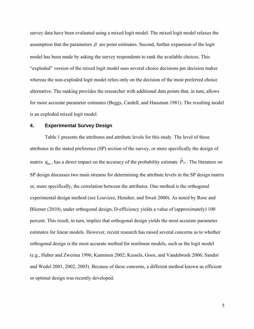
4. Experimental Survey Design

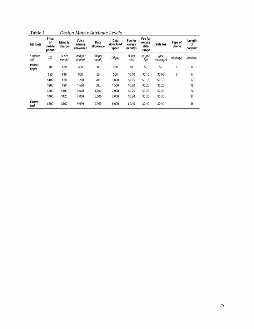
Table 1 presents the attributes and attribute levels for this study. The level of these

attributes in the stated preference (SP) section of the survey, or more specifically the design of

matrix itnq , has a direct impact on the accuracy of the probability estimate inP . The literature on

SP design discusses two main streams for determining the attribute levels in the SP design matrix

or, more specifically, the correlation between the attributes. One method is the orthogonal

experimental design method (see Louviere, Hensher, and Swait 2000). As noted by Rose and

Bliemer (2010), under orthogonal design, D-efficiency yields a value of (approximately) 100

percent. This result, in turn, implies that orthogonal design yields the most accurate parameter

estimates for linear models. However, recent research has raised several concerns as to whether

orthogonal design is the most accurate method for nonlinear models, such as the logit model

(e.g., Huber and Zwerina 1996; Kanninen 2002; Kessels, Goos, and Vandebroek 2006; Sandor

and Wedel 2001, 2002, 2005). Because of these concerns, a different method known as efficient

or optimal design was recently developed.

6

Rose et al. (2008) proposed a Monte Carlo simulation-based efficient design method. In

this method, the analyst initially populates the design matrix randomly. Using parameter priors

from a pilot model, the analyst calculates the choice probabilities for this particular design and

then constructs the asymptotic variance-covariance (AVC) matrix. To evaluate the statistical

efficiency of this initial design, the initial D-error is calculated. This is the determinant of the

AVC matrix from the initial design. In a next step, Rose et al. proposed a design change (i.e.,

changing one or more attributes in the SP design matrix) and then recalculating the D-error. If

the D-error of the second run is smaller than the D-error of the initial run, the second design is

retained; otherwise, it is rejected. This looping procedure is repeated R times up to the point

where the researcher is satisfied with the D-error of the design. The present study employs this

method in deriving the design matrix. The required parameter priors are taken from a pilot study

consisting of 25 completed surveys.

5. Survey Administration

A professional survey firm administered the survey in May 2010 through an omnibus

survey panel consisting of 3.5 million members. In this survey, respondents ranked three

hypothetical mobile service plans (Plan 1, Plan 2, and Plan 3). The full data collection launch

generated 653 survey responses. Of these, 164 surveys were eliminated due to either incomplete

responses or completion times of less than 3.5 minutes. The remaining 489 completed surveys

form the database for this study. In order to ensure valid inferences, the survey data were

examined for consistency and potential biases. Table 2 presents the descriptive statistics for the

survey sample.

7

6. Model Fitting

In the search for the best model, several models were fitted to the survey data. The first

model fits the data to the standard exploded logit model. This model focuses on the choice

behavior of the average consumer. Thus, it does not consider sociodemographic variables, which

serve to forecast beyond the mean. Economic theory postulates that consumers consider all price

attributes when making their purchase decisions. Hence, all mobile service plan attributes are

included in this model. Voice overage charges, however, are expected to be statistically

insignificant. With time counters included in most mobile phones, consumers have direct control

over their monthly voice minute consumption. Consequently, the hypothesis is that subscribers

purchase mobile service plans that include sufficiently large monthly voice allowances, thereby

not requiring voice overage charges. This hypothesis is consistent with Consumer Reports (2011)

that reported finding that 33 percent of US mobile subscribers consume less than half of their

monthly voice allowance. This is in stark contrast to data overage charges that are expected to be

statistically significant. Subscribers generally do not know how much data they consume on a

monthly basis because they do not understand the data requirements of a website download or an

email correspondence.

With an average monthly mobile voice consumption of approximately 700 minutes (FCC

2010; CTIA 2011), the marginal utility that subscribers derive from plans that offer less minutes

than this consumption level might differ from plans that exceed this level. To test this latter

hypothesis, Model 1 includes a dummy variable (dummy_high) that takes the value of one if the

monthly voice allowance exceeds 700 minutes and zero otherwise.

Considering several diagnostic tests, this first model fits the data well. As shown in Table

3, of the 11 coefficients, eight are significant at the 99 percent confidence level and two are

8

significant at 95 percent. As hypothesized, at 18 percent, the overage charge for voice service

(v_over) is statistically insignificant. Furthermore, the signs of the model coefficients correspond

with economic theory. The variable for voice overage charges (v_over) is statistically not

different from zero and not considered further.

Model 1 assumes a zero variance for all parameter estimates. Model 2 relaxes this

assumption by fitting a mixed exploded logit model with all coefficients distributed lognormal.

This model enhancement remedies the IIA problem and allows for consumer-specific

parameters. Relative to the normal distribution, the lognormal distribution has positive values

only and eliminates the possibility of a sign change within a random parameter estimate. In

essence, it ensures that the share < 0 is always zero. Table 4 presents the estimated parameters of

the underlying normal distribution of Model 2. These coefficients are the log values of the

lognormal coefficients. As such, they have no direct interpretation by themselves and only serve

to examine the specifications of the resulting lognormal coefficients. Although the mean

coefficient estimates differ from the estimates in Model 1, there is no apparent drift in values and

only a slight change in statistical significance. Based on a likelihood ratio (LR) index, Model 2

explains the decisions taken by the survey respondents more accurately and therefore provides a

superior fit relative to Model 1. All the coefficients for the mean parameters in Model 2 carry the

expected signs and with the exception of data overage charge (d_over) are all statistically

significant. Similarly, the coefficients for the standard deviations are statistically significant with

the exception of d_over. A univariate Wald test examines whether specifying the coefficient for

d_over_neg as nonstochastic (null hypothesis) yields a model that is superior to Model 2. The

critical value for the chi-square distribution with one degree of freedom at the 1 percent

9

significance level is 6.64. The Wald test finds a score of 2.67 and thus cannot reject the null

hypothesis. Hence, the variable d_over is specified as nonstochastic.

Thus far, the fitted models focused on the attributes of the hypothetical choices only. The

standard deviations of Model 2 indicated that with the exception of d_over survey respondents

differed in their reactions to changes in attribute levels. This raises the question whether

sociodemographic differences explain these taste variations and whether adding these variables

to Model 2 would further improve the model fit. As discussed in the literature review section, the

existing literature provides little guidance as to which sociodemographic variables should be

included in the model, if any.

Although different in significant aspects, the present study is most similar to the studies

of Iimi (2005) and Tripathi and Siddiqui (2009). Neither of these studies found

sociodemographic variables to be statistically significant. The latter study, however, reported

different coefficient estimates by age and gender. Age and gender appear to be the most

frequently considered sociodemographic variables in the literature. Income also was frequently

considered but only in studies that examined aggregate levels of mobile demand, such as a cross-

country comparison (e.g., Garbacz and Thompson 2007). Importantly, income was not

considered in studies where the consumer was the unit of analysis. Thus, Model 3 adds age and

gender as fixed coefficient variables to Model 2. For this, the variable age is interacted with

phone and divided by 10,000. The variable gender is interacted with mrc and divided by 1,000.

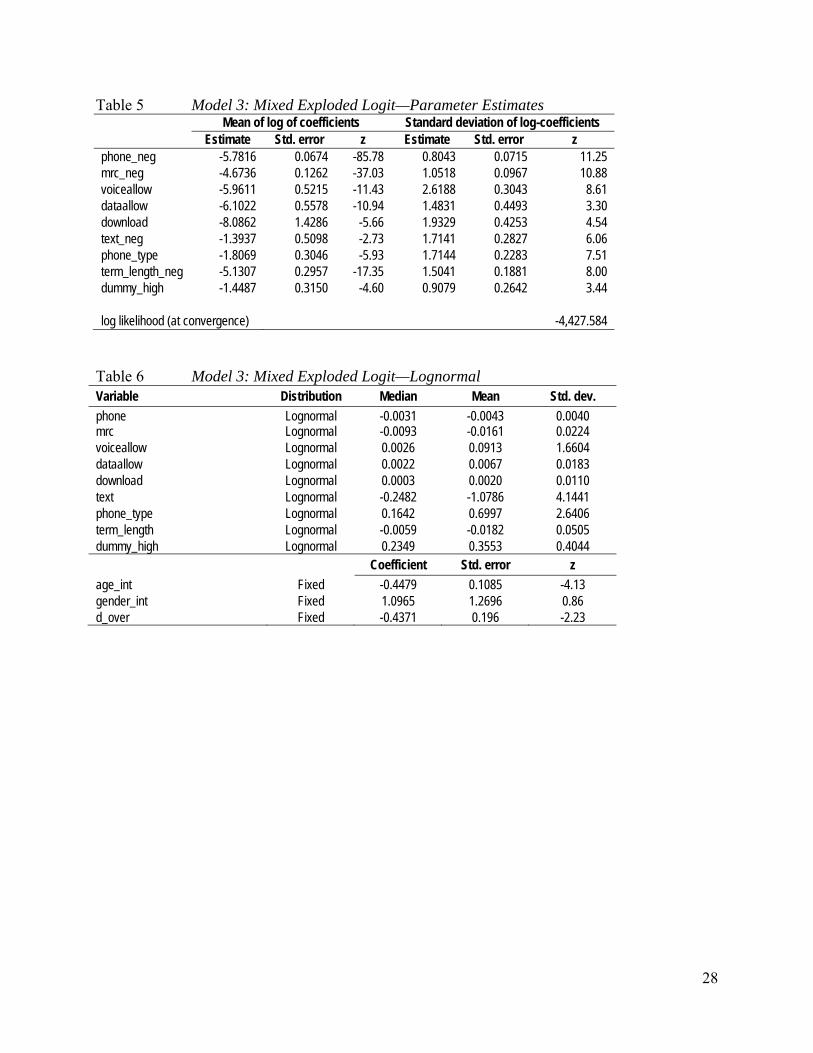
Tables 5 and 6 present the parameter estimates and lognormal medians, means, and standard

deviations for Model 3.

The LR score that compares Model 2 (restricted) to Model 3 (unrestricted) rejects the null

hypothesis that these socioeconomic variables have coefficients of zero. The LRT rejects

10

removing gender_int, which shows a low Z-score in its parameter estimate. Consequently,

adding the sociodemographic variables to Model 2 further improves the model fit. This finding

also provides some resolution to the relevant literature as it provides direct proof of the relevancy

of sociodemographic variables.

7. Results Interpretation

The findings of this study, summarized in Table 6, clearly demonstrate that subscribers

consider far more than the mobile phone when selecting a mobile service plan. In fact,

subscribers consider most, if not all, of the pertinent aspects of the mobile service bundle.

Specifically, the study confirms that subscribers consider the price of the mobile phone where

higher mobile phone prices make a service bundle less attractive (mean: -0.0043, standard

deviation: 0.0040). This, however, does not imply that the “device is King” as has repeatedly

been reported in other studies. Rather, mobile subscribers also consider the monthly recurring

charge where higher monthly charges make a service bundle less attractive (mean: -0.0161,

standard deviation: 0.0224). The number of monthly voice minutes included in the mobile

service plan is also an important demand driver where more minutes make a service bundle more

attractive (mean: 0.0913, standard deviation: 1.6604). The amount of monthly data uploads and

downloads included in the mobile service plan further drives demand with more kilobytes

making a service bundle more attractive (mean: 0.0067, standard deviation: 0.0183). Subscribers

also consider network download speeds where higher speeds make a service bundle more

attractive (mean: 0.0020, standard deviation: 0.0110).

Beyond the mobile phone and MRC, other price factors also feature prominently in the

subscribers’ purchase decisions. These include the charge per kilobyte of data uploads and

downloads in excess of the monthly data upload and download allowance where higher prices

11

make a service bundle less attractive (mean: -0.4371, standard deviation: n/a) and the charge for

SMS where higher prices make a service bundle less attractive (mean: -1.0786, standard

deviation: 4.1441). Consumers clearly prefer smartphones to non-smartphones (mean: 0.6997,

standard deviation: 2.6406) and dislike longer term contracts over shorter commitments (mean: -

0.0182, standard deviation: 0.0505). Finally, subscribers find service plans offering more than

700 minutes per month (the national average) more attractive than plans with a lower monthly

voice allowance (mean: 0.3553, standard deviation: 0.4044).

Decision making differs by age and gender. For each additional year of age, subscribers

become approximately 1 percent more sensitive to changes in mobile phone prices. Women are

approximately 7 percent less sensitive to changes in MRCs.

The significance of this first set of findings is that researchers and policy makers must

examine mobile demand as part of a bundled offering instead of analyzing bundle components

on a standalone basis, as has been the case thus far. Alternatively, if justifiable, researchers must

ensure that other service attributes are constant throughout the study.

Beyond interpreting the number of significant independent variables and the signs of the

coefficients, independent interpretation of the coefficients provides little insight. Rather, relative

interpretation of the logit coefficients is required. Relative interpretation assesses the impact on

utils of one independent variable compared to the impact on utils of another independent

variable. It allows for a richer interpretation of core issues than individual coefficient analysis

and provides unique practical insights. Table 7 presents all possible relative coefficient

interpretations for Model 3.

Relative coefficient interpretation reveals the subscriber’s marginal willingness to pay for

an attribute relative to another attribute. Not all comparisons are meaningful or find applicability

12

in the marketplace. Hence, this analysis focuses only on a subset of the possible combinations.

The core issues for strategy, policy, and regulation often include the price for the mobile phone

and the MRC. This is not a coincidence as these price attributes represent the highest unit charge

in a mobile service plan. Other price components, such as the price of SMS, are mainly usage

driven. Hence, the natural argument is to examine the trade-off space or util-equivalent space

relative to these price attributes. Specifically, the relative interpretation of mrc relative to phone

is examined first. This analysis is followed by the relative interpretation of phone_type and

phone and also term_length and phone. The variables voice_allow, data_allow, download,

d_over, and text are evaluated relative to mrc.

The MRC coefficient reveals that average subscribers are indifferent between a $1

change in the MRC and a $3.74 equidirectional change in the mobile phone price. As the cost of

a mobile phone is a one-time fee and the MRC is a recurring charge, this implies that such

subscribers amortize their mobile phones over approximately four months. Over the life of a

two-year contract, a total discount in MRC of $24 is equivalent to an upfront discount of $3.74.

This implies a discount rate of 25.9 percent. This result is consistent with the previous relevant

literature. For instance, Hausman (1979), in examining individual discount rates in the purchase

and utilization of energy-using durables, found a discount rate of 20 percent. Similarly, Dubin

and McFadden (1984) found a discount rate of 20.5 percent for electric appliances. In addition,

Hausman (2002) discussed the importance of these trade-offs in the development of mobile

telecommunications demand.

The relative interpretation of the coefficient for the mobile phone price and the mobile

phone type finds a marginal willingness to pay for smartphones of $163 over non-smartphones.

13

This finding is generally consistent with the price differential between smartphones and non-

smartphones observed in the marketplace.

Service providers commonly impose term contracts with early termination fees (ETFs) to

compensate for mobile phone subsidies. The relative interpretation of the mobile phone price and

the term length coefficients reveals that average-aged subscribers are willing to pay an additional

$4.23 for each month deducted from a term contract. A typical term contract is 24 months.

Assuming a linear relationship, this implies that average-aged subscribers are willing to pay an

additional 24 x $4.23 = $101.52 for the mobile phone in order to avoid a term contract.

Conversely, the average subscriber prefers a term contract of 24 months to paying the full retail

price for a mobile phone for all mobile phones offered at a discount of $101 or more.

Closely linked to the MRC is the number of monthly voice minutes included in a mobile

service plan. Model 3 reveals a willingness to pay of approximately $0.06 for both male and

female subscribers. This is almost eight times the voice overage charge but consistent with the

price subscribers pay on average under their monthly voice allowance. Consequently, subscribers

are not willing to pay a premium for voice minutes consumed beyond their monthly voice

allowance. This means that subscribers purchase service plans that include a sufficient number of

voice minutes. Hence, as observed, voice overage charges do not contribute in a statistically

significant manner to mobile service plan selection.

Model 3 also finds that both male and female subscribers are willing to pay an additional

$0.42 and $0.45, respectively, in the MRC for each additional 100 kilobytes (kB) of data

allowance. AT&T charges subscribers without a data plan $2.00 per megabyte (MB) of data

(http://www.att.com). At 1,024 kB per MB, this translates to $0.20 per kB. Similarly, Verizon

Wireless charges $0.19 per kB of data for pay-as-you-go data subscribers. Hence, Model 3 finds

14

a mean willingness to pay for additional data allowances that is higher than prices in the

marketplace. Similarly, subscribers are willing to pay an additional $2.71 a month for each $0.10

change in the per kB data overage charge. Unlike voice overage charges (which are invoiced per

minute), service providers typically invoice data overage charges in rather large increments. For

instance, for subscribers who exceed the 75 MB data allowance of the $10 data plan, Verizon

Wireless bills the subscriber $10 for an additional 75 MBs of data. This overage charge applies

regardless of whether the subscriber exceeded the data plan allowance by one byte or the entire

additional 75 MBs. Assuming that the average subscriber who incurs a data overage charge uses

half of this overage allowance, this implies that Verizon charges $10 ÷ (75 ÷ 2) = $0.27 per MB,

or $0.0003 per kB. In order to avoid this data overage charge, subscribers appear to be willing to

pay only a fraction of a cent increase in the MRC. Stated differently, subscribers are not willing

to increase their MRC to avoid data overage charges. In contrast to voice overage charges, this

result implies that subscribers are willing to incur data overage charges.

As found by Dippon (2010), the current download speed impediments of 3G mobile

service are a significant deterrent of 3G take-up. Model 3 demonstrates that subscribers are

willing to pay an additional $0.12 in the MRC for each additional 100 kilobits per second (kbps)

download speed. At current mobile speeds of approximately 1,000 kbps, service providers that

can increase their mobile download speeds from the current levels to 5,000 kbps, thus making

them comparable to standard DSL service, can charge an additional (4,000 ÷ 100) x 0.12 =$4.80

in the MRC. Long-term evolution (LTE), often referred to as 4G, promises rates far in excess of

standard DSL. Verizon Wireless recently announced that its 4G network delivers 5,000–12,000

kbps when downloading data (http://www.verizonwireless.com). If so, average subscribers

15

appear to be willing to pay a premium ranging from $4.80 to $13.20 per month to enjoy this

service.

US service providers offer SMS on both a pay-per-use and a plan basis. For instance,

AT&T Mobility, Verizon Wireless, and other service providers offer SMS at $0.20 per SMS sent

and received. AT&T Mobility offers a $10 plan that includes 1,000 SMSs and a $20 plan that

provides unlimited SMSs. The former plan implies an SMS rate of $0.10 per SMS. Model 3

reveals that male subscribers are indifferent between a $0.10 change per SMS and a $6.70

equidirectional change in the MRC. For female subscribers, this amount is $7.19. This implies

that non-plan subscribers (who currently pay $0.20) are willing to pay $13.40 (male) and $14.38

(female) for an unlimited plan. Similarly, non-plan subscribers are willing to pay $6.70 (male)

and $7.19 (female) to reduce their SMS rate to $0.10. These two findings indicate that AT&T

Mobility’s prices for its SMS plans are higher than the subscribers’ mean willingness to pay for

this bundle component, as found by Model 3. The findings of Model 3 are more in line with the

pricing structure of T-Mobile that offers unlimited SMS for $10 a month, slightly below the

indicated mean willingness to pay.

8. Strategy Implications

Random draws from the underlying normal distribution of the mixed logit model generate

the probabilities that an average subscriber will select a specific service plan. Attributing these

probabilities to the service providers yields forecasted market shares.

Table 8 summarizes the attribute levels of an illustrative market simulation with four

service providers (Provider 1, Provider 2, Provider 3, and Provider 4) along with the average

logit probabilities, or market shares. Each service provider is assumed to offer only the plan

16

shown in the default scenario. The objective of this market simulation is to examine the market

share gains and losses occurred by Provider 1 from deviating from the default scenario.

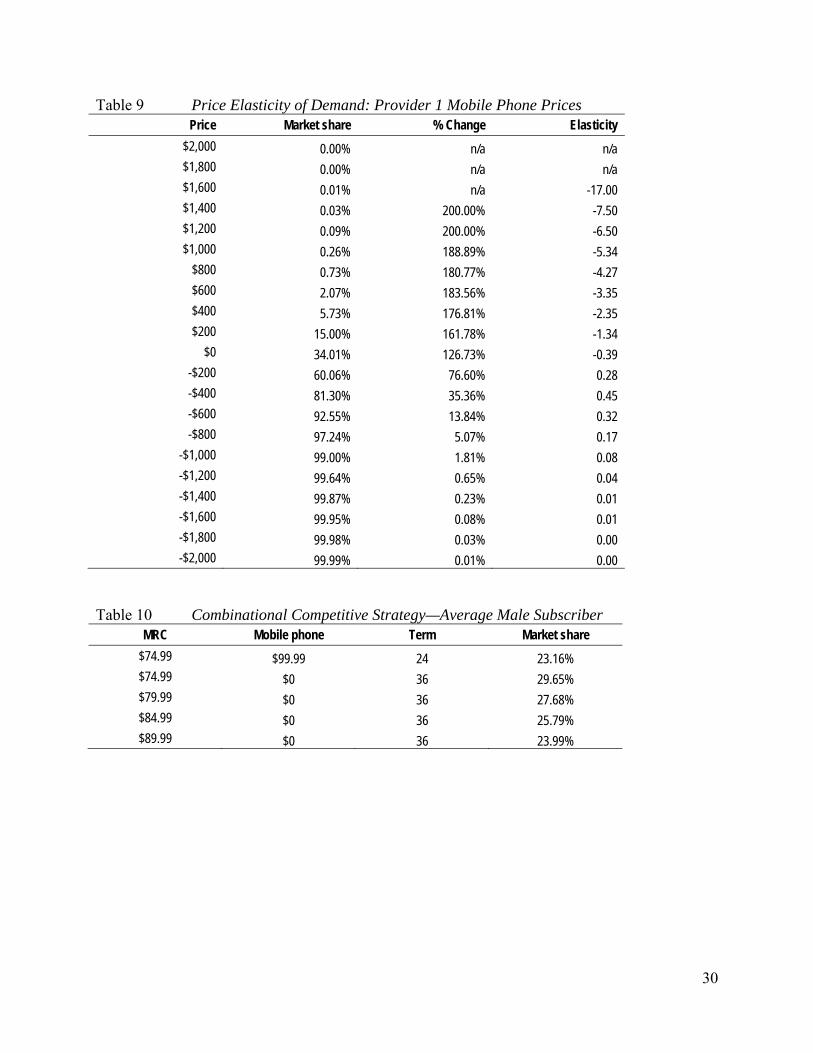
A first possible competitive strategy for Provider 1 is to vary mobile phone prices. An

increase or decrease in the current illustrative mobile phone price for Provider 1 results in

different market shares for the service provider. Table 9 summarizes the market share as a

function of price and calculates the elasticity of demand for changes in mobile phone prices. The

price elasticity of demand for Provider 1’s service plan reveals that with a mobile phone price of

approximately $200 and higher the service provider faces elastic demand (unit elasticity is at

$258). In this range of the demand curve, the percentage of the market share change is greater

than the percentage price decrease. Practically, this finding means that if the service provider

were to increase mobile phone prices, it could minimize the market share impact of this change

by remaining in the inelastic range of the demand curve.

Alternatively, Provider 1 could change its MRC by increasing or decreasing it. This

analysis reveals that at the default price ($74.99) and above the service provider faces elastic

demand. In this range of the demand curve, the market penalizes service operators that seek to

increase the MRC and rewards those that decrease their prices (albeit, possibly only in the short

run).

Provider 1 could also alter its term contract requirements. However, the price elasticity of

demand with respect to term length is inelastic in the range of zero to 36 months. This implies, at

least in this hypothetical setting, that as a standalone strategy decreasing the term length from its

current 24 months is not an effective competitive strategy. In contrast, the inelastic region of the

demand curve between 24 months and 36 months might provide a profit opportunity for Provider

1.

17

Although strategies that are more competitive exist, an effective strategy could also entail

altering more than one service attribute. For instance, in Table 10, a combinational strategy for

Provider 1 is examined. In this strategy, Provider 1 increases the term length to 36 months,

provides a free mobile phone, and varies increases in the MRC to obtain a positive net effect. In

the default scenario, Provider 1 has a market share of 23.16 percent. Offering free mobile phones

and increasing the term length to 36 months boosts the service provider’s market share by 28 to

29.65 percent. At this rate, Provider 1 must bear the revenue loss from offering free mobile

phones. If it increased the MRC by $5 per month over the previous scenario, it would retain a

market share of 27.68 percent. This is still higher than the default market share by 20 percent. By

increasing revenue by $5 per month, Provider 1 increases revenue by $5 x 36 = $180 over the

subscriber’s lifetime. Offsetting the mobile phone subsidy of $99.99, this yields a net revenue

increase of $80.01 per subscriber in addition to the 4.5 points market share gain. Additionally,

Provider 1 lowers its churn rate by contractually obligating subscribers to remain with the carrier

for an additional 12 months beyond the original 24 months.

Given the high level of competition in the US mobile market, other service providers are

likely to follow suit, thereby cancelling the long-term benefits from competitive strategies.

However, due to the term-length requirements, service providers that pioneer a profitable

strategy stand to enjoy a two- to three-year first-mover advantage.

9. Policy Implications

The study’s findings also provide valuable information on a number of critical policy

decisions pending before the FCC and state regulators. Most generally, the regulators must

consider the entire service bundle when examining market behavior or alleged market failures.

Considering individual service attributes in isolation yields incorrect results and thus incorrect

18

regulation and policy. For instance, the FCC and US Congress still discuss term contracts

separate from all other service attributes.

Policy makers, as well as several class action plaintiffs, accuse AT&T Mobility, Verizon

Wireless, Sprint, and others of harming subscribers by requiring term contracts with ETFs. The

allegations do not consider that these service providers offer term contracts in conjunction with

several other attributes. Similarly, MetroPCS, a regional service provider, currently airs

advertisements in which it promotes its absences of “stupid term contracts.”

The relative evaluation of the coefficients for the mobile phone price and the MRC has

shown a marginal willingness to pay of $101 in terms of mobile phone prices to avoid a term

contract. However, a closer look at MetroPCS’ mobile phone pricing structure finds prices that

exceed by more than $101 the prices of other service providers that demand term contracts. For

instance, MetroPCS sells the smartphone BlackBerry Curve 8530 for $199 without a contract

(see http://metropcs.com). AT&T Mobility sells the same handset for $0.01 with a two-year

contract (see http://www.att.com). Similarly, Verizon Wireless sells the handset for $79.99 (see

http://www.verizonwireless.com). Hence, from a welfare perspective, MetroPCS’ offering is

inferior to the offerings by these other service providers. Yet, due to the incorrect analysis of

ETFs, MetroPCS is not subject to the federal investigation. This study also demonstrates that

varying the term lengths from zero months to 36 months has little impact on subscribers’

decisions because all changes within this range fall in the inelastic range of the demand curve.

This study highlights the importance of offering spectrum that, in turn, will increase

mobile upload and download speeds. Specifically, subscribers are willing to pay a premium of up

to $13.20 over the current MRC in order to obtain LTE mobile speeds. With most unlimited data

plans around $30 per month, this implies that subscribers are willing to increase their MRC by

19

45 percent in order to obtain LTE. The high willingness to pay illustrates the high priority that

subscribers place on the increase in mobile upload and download speeds. The move to LTE

could also have an impact on fixed-line broadband offerings. Currently, fixed-line broadband

providers, such as Comcast, offer comparable Internet access at $34.99 per month

(http://www.comcast.com). With consumers willing to pay $43.20 for mobile broadband

offerings, subscribers place an $8.21 premium on mobile broadband relative to fixed-line

broadband. Hence, fixed-line broadband providers will need to price their services at a

differential larger than the $8.21 premium in order to maintain their subscriber base.

Finally, as is the case in all other investigations, this study clearly shows that SMS

pricing is only one attribute of the service bundle. Competition occurs at the service bundle level.

Consequently, bundles that include discounted SMS prices directly compete with bundles that

charge $0.20 for each additional SMS.

10 Conclusions

Counter to casual observation, this study reveals that consumers consider far more than

simply the mobile phone when selecting mobile phone service. In fact, consumers carefully

consider most, if not all, of the pertinent aspects of the mobile service bundle, including mobile

phone price, monthly recurring charge, monthly voice and data minutes included in the plan,

mobile upload and download speeds, data overage charges, SMS prices, the type of mobile

phone offered, and the length of the term contract. This study also reveals the trade-offs that

subscribers make when selecting among the many attributes of a mobile phone plan.

This new understanding of choice making allows for important strategy and policy

conclusions. In terms of strategy, the study demonstrates how service providers can generate a

profit, at least in the short run, by deviating from this apparent market equilibrium. The study’s

20

findings also provide valuable information on a number of critical policy decisions pending

before the FCC and state regulators. Specifically, the FCC and state regulators must analyze all

relevant attributes simultaneously to capture important and complex trade-offs between

attributes.

A fundamental change is occurring in the mobile communications market. While

traditionally used for voice communications only, the technological evolution has expanded

mobile services far beyond simple voice calling. The findings of this study highlight that

researchers, service providers, and regulators must adapt to this changing environment by

considering mobile communications not as a collection of individual services and service

components but an all-encompassing communications bundle.

References

Ahn, J.-H., S.-P. Han, and Y.-S. Lee. 2006. “Customer churn analysis: churn determinants and

mediation effects of partial defection in the Korean mobile telecommunications service

industry.” Telecommunications Policy 30:552–568.

Beggs, S., S. Cardell, and J. Hausman. 1981. “Assessing the potential demand for electric cars.”

Journal of Econometrics 16:1–19.

Consumer Reports. “Cut your cell-phone costs.” Consumer Reports.Org. Last modified January

2011. http://www.consumerreports.org/cro/magazine-

archive/2011/january/electronics/best-cell-phones/cell-phone-costs/index.htm.

CTIA. 2011. “Wireless in America.” Accessed May 12, 2011.

http://files.ctia.org/pdf/HowWirelessWorks_jan2011.pdf.

Dewenter, R., and J. Haucap. 2008. “Demand elasticities for mobile telecommunications in

Austria.” Journal of Economics and Statistics (Jahrbuecher fuer Nationaloekonomie und

21

Statistik) 228:49–63.

Dippon, C. 2010. “Is faster necessarily better? Third generation (3G) take-up rates and the

implication for next generation services.” Paper presented at the International

Telecommunications Society 18th Biennial and Silver Anniversary Conference, Tokyo,

June 27–30.

Dubin, J. A., and D. L. McFadden. 1984. “An econometric analysis of residential electric

appliance holdings and consumption.” Econometrica 52:345–362.

Eshghi, A., D. Haughton, and H. Topi. 2007. “Determinants of customer loyalty in the wireless

telecommunications industry.” Telecommunications Policy 31:93–106.

FCC. 2010. Fourteenth Report. 25 FCC Rcd 11407.

Garbacz, C., and H. Thompson. 2007. “Demand for telecommunication services in developing

countries.” Telecommunications Policy 31:276–289.

Grzybowski, L., and P. Pereira. 2008. “The complementarity between calls and messages in

mobile telephony.” Information Economics and Policy 20:279–287.

Hausman, J. 1979. “Individual discount rates and the purchase and utilization of energy-using

durables.” The Bell Journal of Economics 10:33–54.

Hausman, J. 1999. “Cellular telephone, new products, and the CPI.” Journal of Business &

Economic Statistics 17:188–194.

Hausman, J. 2002. “Mobile telephone.” In Handbook of Telecommunications Economics, edited

by M. Cave, S. K. Majumdar, and I. Vogelsang. Amsterdam: North-Holland. ISBN 978-

0444503893.

Huber, J., and K. Zwerina. 1996. “The importance of utility balance in efficient choice designs.”

Journal of Marketing Research 33:307–317.

22

Iimi, A. 2005. “Estimating demand for cellular phone service in Japan.” Telecommunications

Policy 29:3–23.

Ishii, K. 2004. “Internet use via mobile phone in Japan.” Telecommunications Policy 28:43–58.

Kanninen, B. J. 2002. “Optimal design for multinomial choice experiments.” Journal of

Marketing Research 39:214–217.

Katz, J. E., and S. Sugiyama. 2005. “Mobile phones as fashion statements: the co-creation of

mobile communication’s public meaning.” In Mobile communications: re-negotiation of

the social sphere, edited by R. Ling and E. Pedersen, 63–81. London: Springer. ISBN 978-

1-852-33931-9.

Kessels, R., P. Goos, and M. Vandebroek. 2006. “A comparison of criteria to design efficient

choice experiments.” Journal of Marketing Research 43:409–419.

Kim, M.-K., M.-C. Park, and D.-H. Jeong. 2004. “The effects of customer satisfaction and

switching barrier on customer loyalty in Korean mobile telecommunications services.”

Telecommunications Policy 28:145–159.

Kim, Y., R. Telang, W. Vogt, and R. Krishnan. 2010. “An empirical analysis of mobile voice

service and SMS: a structural model.” Management Science 56:234–252.

Lemish, D., and A. A. Cohen. 2005. “Tell me about your mobile and I will tell you who you are:

Israelis talk about themselves.” In Mobile communications: re-negotiation of the social

sphere, edited by R. Ling and E. Pedersen, 187–202. London: Springer. ISBN 978-1-852-

33931-9.

Louviere, J. J., D. A. Hensher, and J. D. Swait. 2000. Stated choice methods—analysis and

application. Cambridge, England: University of Cambridge. ISBN 0-521-78275-9.

McFadden, D. 1974. “Conditional logit analysis of qualitative choice behavior.” In Frontiers in

23

econometrics, edited by P. Zarembka, 105–142. New York: Academic Press. ISBN 978-

0127761503.

Ozcan, Y., and K. Kocak. 2003. “Research note: a need or a status symbol? Use of cellular

telephones in Turkey.” European Journal of Communication 18:241–254.

Rose, J. M., and M. C. J. Bliemer. 2010. “Stated choice experimental design theory: the who, the

what and the why.” Unpublished manuscript, University of Sydney, Sydney, Australia.

Rose J. M., M. C. J. Bliemer, D. A. Hensher, and A. T. Collins. 2008. “Designing efficient stated

choice experiments in the presence of reference alternatives.” Transportation Research

42:395–406.

Sandor, Z., and M. Wedel. 2001. “Designing conjoint choice experiments using managers’ prior

beliefs.” Journal of Marketing Research 38:430–444.

Sandor, Z., and M. Wedel. 2002. “Profile construction in experimental choice designs for mixed

logit models.” Marketing Science 21:455–475.

Sandor, Z., and M. Wedel. 2005. “Heterogeneous conjoint choice designs.” Journal of Marketing

Research 42:210–218.

Tallberg, M., H. Hammainen, J. Toyli, S. Kamppari, and A. Kivi. 2007. “Impacts of mobile

phone bundling on mobile data usage: the case of Finland.” Telecommunications Policy

31:648–659.

Train, K. 1993. Qualitative choice analysis, theory, econometrics, and application to automobile

demand. Cambridge, MA: MIT Press. ISBN 0-262-20055-4.

Train, K. 2009. Discrete choice methods with simulation. 2nd ed. Cambridge, England:

Cambridge University Press. ISBN 978-0-521-74738-7.

Tripathi, S., and M. Siddiqui. 2009. “An empirical investigation of customer preferences in

24

mobile services.” Journal of Targeting, Measurement and Analysis for Marketing 18:49–

63.

Turel, O., A. Serenko, and N. Bontis. 2007. “User acceptance of wireless short messaging

services: deconstructing perceived value.” Information and Management 44:63–73.

25

Table 1 Design Matrix Attribute Levels

Attribute

Price of

mobile phone

Monthly charge

Voice minute

allowance

Data allowance

Data download

speed

Fee for excess minutes

Fee for excess

data usage

SMS fee Type of phone

Length of

contract

Attribute unit

($) ($ per month)

(min per month)

(kb per month)

(kbps) ($ per min)

($ per kb)

(per message)

(dummy) (months)

Values begin

$0 $20 400 0 250 $0 $0 $0 1 0

$50 $40 800 50 500 $0.10 $0.10 $0.05 0 6

$100 $60 1,200 200 1,000 $0.15 $0.15 $0.10 12

$200 $80 1,600 500 1,500 $0.20 $0.20 $0.20 18

$300 $100 2,000 1,000 2,000 $0.25 $0.25 $0.25 24

$400 $120 3,000 5,000 3,000 $0.30 $0.30 $0.30 30

Values end

$500 $160 9,999 9,999 6,000 $0.40 $0.40 $0.40 36

26

Table 2 Sample Descriptive Statistics Variable Obs Mean Std. dev. Min Max Median Skew. Kurtosis 25% 75% Attribute levels

Q1: Age 489 44.43 15.45 18 82 42 0.31 2.11 31 55

Q2: Wireless 489 1.06 0.23 1 2 1 3.81 15.53 1 1 Yes=1, No=2

Q3: Fin. responsibility 489 1.13 0.33 1 2 1 2.24 6.03 1 1 Yes=1, No=2

Q4: Plan minutes 417 3.93 2.01 1 8 4 0.31 1.85 2 6

<400 = 1, 400-699=2, 700-899=3, 900-1399=4, 1400-2099=5, Unlim=6, Prepaid=7, Don't know=8

Q5: Data plan subscription 417 1.58 0.49 1 2 2 (0.34) 1.11 1 2 Yes=1, No=2

Q6: SMS plan subscription 417 1.54 0.50 1 2 2 (0.15) 1.02 1 2 Yes=1, No=2

Q7: Mobile Internet usage 417 1.60 0.49 1 2 2 (0.41) 1.17 1 2 Yes=1, No=2

Q8: Mobile email usage 417 1.62 0.49 1 2 2 (0.48) 1.23 1 2 Yes=1, No=2

Q9: Monthly expenses 417 2.13 1.00 1 5 2 0.72 2.90 1 3

<$50=1, $50-$99=2, $100-$149=3, >$150=4, Don't know=5

Q10: Term contract 417 1.32 0.51 1 3 2 1.23 3.45 1 2 Yes=1, No=2, Don't know =3

Q11: Landline subscriber 489 1.28 0.45 1 2 1 0.98 1.96 1 2 Yes=1, No=2

Q12: State of residence 489 25.45 16.00 1 51 24 0.04 1.46 10 43

Q13: Residence density 489 2.30 0.84 1 4 2 0.01 2.29 2 3

Metropolitan=1, Suburban=2, Small town=3, Farming =4

Q14: Education 489 3.18 1.03 1 5 3 0.03 1.77 2 4

<High school =1, High school=2, Vocational =3, College = 4, Post-graduate = 5

Q15: Employment status 489 1.90 0.92 1 3 2 (0.15) 1.02 1 3 Full-time = 1, Part-time = 2, Not employed = 3

Q16: Gender 489 1.53 0.50 1 2 2 (0.41) 1.17 1 2 Male = 1, Female = 2

Q17 Marital status 489 1.79 0.75 1 4 2 (0.48) 1.23 1 2

Single = 1, Married = 2, Partnered = 3, Other = 4

Q18: Number of children 489 1.56 0.93 1 4 2 0.72 2.90 1 2 Zero = 1, One = 2, Two = 3, More than three = 4

Q19: Annual income 489 2.34 1.11 1 6 1 1.23 3.45 1 3

<$30K=1, $30K-$49K=2, $50K-$74K=3, $75K-$149K=4, >$150K=5, No answer=6

27

Table 3 Model 1: Exploded Logit Number of obs 14670

Number of groups 5868

Obs per group

min 2.00

average 2.50

max 3.00

LR chi2(10) 1018.17

Prob > chi2 0.00

Log likelihood -4747.94

select Coefficient Std. Error z P>|z| 95% Conf. interval

phone -0.0026 0.0001 -24.390 0.000 -0.0028 -0.0024

mrc -0.0084 0.0004 -19.070 0.000 -0.0093 -0.0075

voiceallow (per 100) 0.0045 0.0012 3.740 0.000 0.0021 0.0068

dataallow (per 100) 0.0034 0.0007 4.530 0.000 0.0019 0.0048

download (per 100) 0.0019 0.0009 2.100 0.036 0.0001 0.0036

v_over 0.0365 0.1644 0.220 0.824 -0.2858 0.3588

d_over -0.3083 0.1489 -2.070 0.038 -0.6001 -0.0165

text -0.6225 0.1212 -5.140 0.000 -0.8601 -0.3849

phone_type 0.2956 0.0351 8.420 0.000 0.2268 0.3644

term_length -0.0097 0.0014 -7.160 0.000 -0.0124 -0.0071

dummy_high 0.3972 0.0475 8.360 0.000 0.3041 0.4904

Table 4 Model 2: Mixed Exploded Logit—Parameter Estimates

Mean of log-coefficients Standard deviation of log-

coefficients Estimate Std. error z Estimate Std. error z

phone_neg -5.8077 0.0691 -84.0478 0.8481 0.0653 12.9877

mrc_neg -4.7468 0.0976 -48.6352 1.1018 0.0926 11.8985

voiceallow -6.0218 0.5553 -10.8442 2.7094 0.308 8.79675

dataallow -6.0708 0.4371 -13.8888 1.4404 0.2851 5.05226

download -7.6611 1.1188 -6.8476 1.7945 0.3488 5.14478

d_over_neg -1.2328 0.7544 -1.63415 0.8723 0.5337 1.63444

text_neg -1.1938 0.4339 -2.75133 1.5716 0.2346 6.69906

phone_type -1.8847 0.3511 -5.36799 1.8261 0.282 6.47553

term_length_neg -5.0726 0.2695 -18.8223 1.4567 0.1603 9.08734

dummy_high -1.5618 0.3581 -4.36135 1.0577 0.2437 4.34017

log likelihood (at convergence) - 4437.43

28

Table 5 Model 3: Mixed Exploded Logit—Parameter Estimates Mean of log of coefficients Standard deviation of log-coefficients

Estimate Std. error z Estimate Std. error z phone_neg -5.7816 0.0674 -85.78 0.8043 0.0715 11.25 mrc_neg -4.6736 0.1262 -37.03 1.0518 0.0967 10.88 voiceallow -5.9611 0.5215 -11.43 2.6188 0.3043 8.61 dataallow -6.1022 0.5578 -10.94 1.4831 0.4493 3.30 download -8.0862 1.4286 -5.66 1.9329 0.4253 4.54 text_neg -1.3937 0.5098 -2.73 1.7141 0.2827 6.06 phone_type -1.8069 0.3046 -5.93 1.7144 0.2283 7.51 term_length_neg -5.1307 0.2957 -17.35 1.5041 0.1881 8.00 dummy_high -1.4487 0.3150 -4.60 0.9079 0.2642 3.44

log likelihood (at convergence) -4,427.584

Table 6 Model 3: Mixed Exploded Logit—Lognormal Variable Distribution Median Mean Std. dev.

phone Lognormal -0.0031 -0.0043 0.0040 mrc Lognormal -0.0093 -0.0161 0.0224 voiceallow Lognormal 0.0026 0.0913 1.6604 dataallow Lognormal 0.0022 0.0067 0.0183 download Lognormal 0.0003 0.0020 0.0110 text Lognormal -0.2482 -1.0786 4.1441 phone_type Lognormal 0.1642 0.6997 2.6406 term_length Lognormal -0.0059 -0.0182 0.0505 dummy_high Lognormal 0.2349 0.3553 0.4044 Coefficient Std. error z

age_int Fixed -0.4479 0.1085 -4.13 gender_int Fixed 1.0965 1.2696 0.86 d_over Fixed -0.4371 0.196 -2.23

29

Table 7 Relative Coefficient Interpretation Model 3 phone mrc voice

allow data allow

down load

d_over text phone type

term length

dummy high

phone 1.00 0.27 -0.05 -0.64 -2.15 0.01 0.00 -0.01 0.24 0.01 mrc

3.74 1.00 -0.18 -2.40 -8.05 0.04 -

0.01 -0.02 0.88 0.05 voiceallow -21.23 -5.67 1.00 13.63 45.65 -0.21 0.08 0.13 -5.02 -0.26 dataallow -1.56 -0.42 0.07 1.00 3.35 -0.02 0.01 0.01 -0.37 -0.02 download -0.47 -0.12 0.02 0.30 1.00 0.00 0.00 0.00 -0.11 -0.01 d_over

101.65 27.15 -4.79 -65.24 -

218.55 1.00 -

0.41 -0.62 24.02 1.23 text -

250.84 -

66.99 11.81 160.99 539.30 -2.47 1.00 1.54 -59.26 -3.04 phone_type -

162.72 -

43.46 7.66 104.43 349.85 -1.60 0.65 1.00 -38.45 -1.97 term_length

4.23 1.13 -0.20 -2.72 -9.10 0.04 -

0.02 -0.03 1.00 0.05 dummy_high

82.63 22.07 -3.89 -53.03 -

177.65 0.81 -

0.33 -0.51 19.52 1.00 Table 8 Default Scenarios and Market Shares

Provider 1 Provider 2 Provider 3 Provider 4

phone 99.99 99.99 0.00 199.99 mrc 74.99 54.99 59.99 69.99 voiceallow (in 100s) 9.00 4.50 9.00 10.00 dataallow (in 100s) 20.48 7.68 0.00 20.48 download (in 100s) 14.10 8.77 7.95 8.68 d_over 0.08 0.27 0.03 0.30 Text 0.20 0.02 0.02 0.00 phone_type 1.00 1.00 0.00 1.00 term 24.00 24.00 24.00 24.00 dummy_high 1.00 0.00 1.00 1.00 logit probability 23.16% 29.19% 32.31% 15.34%

30

Table 9 Price Elasticity of Demand: Provider 1 Mobile Phone Prices Price Market share % Change Elasticity

$2,000 0.00% n/a n/a $1,800 0.00% n/a n/a $1,600 0.01% n/a -17.00 $1,400 0.03% 200.00% -7.50 $1,200 0.09% 200.00% -6.50 $1,000 0.26% 188.89% -5.34

$800 0.73% 180.77% -4.27 $600 2.07% 183.56% -3.35 $400 5.73% 176.81% -2.35 $200 15.00% 161.78% -1.34

$0 34.01% 126.73% -0.39 -$200 60.06% 76.60% 0.28 -$400 81.30% 35.36% 0.45 -$600 92.55% 13.84% 0.32 -$800 97.24% 5.07% 0.17

-$1,000 99.00% 1.81% 0.08 -$1,200 99.64% 0.65% 0.04 -$1,400 99.87% 0.23% 0.01 -$1,600 99.95% 0.08% 0.01 -$1,800 99.98% 0.03% 0.00 -$2,000 99.99% 0.01% 0.00

Table 10 Combinational Competitive Strategy—Average Male Subscriber

MRC Mobile phone Term Market share

$74.99 $99.99 24 23.16% $74.99 $0 36 29.65% $79.99 $0 36 27.68% $84.99 $0 36 25.79% $89.99 $0 36 23.99%