Embed Size (px)
Citation preview
Constructions, Lower Bounds, and New Directions inCryptography and Computational Complexity
by
Periklis A. Papakonstantinou
A thesis submitted in conformity with the requirementsfor the degree of Doctor of Philosophy
Graduate Department of Computer ScienceUniversity of Toronto
Copyright c© 2010 by Periklis A. Papakonstantinou
Abstract
Constructions, Lower Bounds, and New Directions in
Cryptography and Computational Complexity
Periklis A. Papakonstantinou
Doctor of Philosophy
Graduate Department of Computer Science
University of Toronto
2010
In the first part of the thesis we show black-box separations in public and private-key cryptog-
raphy. Our main result answers in the negative the question of whether we can base Identity
Based Encryption (IBE) on Trapdoor Permutations. Furthermore, we make progress towards
the black-box separation of IBE from the Decisional Diffie-Hellman assumption. We also show
the necessity of adaptivity when querying one-way permutations to construct pseudorandom
generators a la Goldreich-Levin; an issue related to streaming models for cryptography.
In the second part we introduce streaming techniques in understanding randomness in effi-
cient computation, proving lower bounds for efficiently computable problems, and in computing
cryptographic primitives.
We observe [Coo71] that logarithmic space-bounded Turing Machines, equipped with an
unbounded stack, henceforth called Stack Machines, together with an external random tape
of polynomial length characterize RP,BPP an so on. By parametrizing on the number of
passes over the random tape we provide a technical perspective bringing together Streaming,
Derandomization, and older works in Stack Machines. Our technical developments relate this
new model with previous works in derandomization. For example, we show that to derandomize
parts of BPP it is in some sense sufficient to derandomize BPNC (a class believed to be much
lower than P ⊆ BPP). We also obtain a number of results for variants of the main model,
regarding e.g. the fooling power of Nisan’s pseudorandom generator (PRG) [Nis92] for the
derandomization of BPNC1, and the relation of parametrized access to NP-witnesses with width-
parametrizations of SAT.
A substantial contribution regards a streaming approach to lower bounds for problems in
ii
the NC-hierarchy (and above). We apply Communication Complexity to show a streaming
lower bound for a model with an unbounded (free-to-access) pushdown storage. In particular,
we obtain a nΩ(1) lower bound simultaneously in the space and in the number of passes over the
input, for a variant of inner product. This is the first lower bound for machines that correspond
to poly-size circuits, can do Parity, Barrington’s language, and decide problems in P − NC
assuming EXP 6= PSPACE.
Finally, we initiate the study of log-space streaming computation of cryptographic prim-
itives. We observe that the work on Cryptography in NC0 [AIK06a] yields a non-black-box
construction of a one-way function computable in an O(log n)-space bounded streaming model.
Also, we show that relying on this work is in some sense necessary.
iii
Acknowledgements
It is a great privilege to study Theory at the University of Toronto. I was also privileged
to have an incredible advisor and PhD committee. I’m most thankful to Charles Rackoff for
his invaluable research supervision, countless discussions, very close attention to my work,
and insightful comments. In addition, Charlie is among the most open and liberal-minded
individuals I have met in academia, which made this process more interesting. I’m also grateful
to the other members of my committee Allan Borodin, Stephen Cook, and Toniann Pitassi for
always been there with useful remarks, research suggestions, and encouragement. Many thanks
to my external thesis reviewer Eric Allender for his detailed remarks and suggestions.
Significant part of the research I have included in the thesis is a result of collaboration,
mostly with people from the University of Toronto. I want to thank my office-mates and col-
leagues, and co-authors (from UofT and elsewhere) Dan Boneh, Mark Braverman, Yuval Filmus,
Michail Flouris, Travis Gagie, Wesley George, Victor Glazer, Costis Georgiou, Kaveh Ghasem-
loo, Hamed Hatami, Ali Juma, Lap Chi Lau, Dai Le, Tsuyoshi Morioka, Phuong Nguyen,
Yevgeniy Vahlis, Brent Waters, and Anastasios Zouzias. Special thanks are due to my friends
and co-authors Matei David and Anastasios Sidiropoulos.
I’d like to thank the faculty from the Department of Mathematics and in particular Pete
Gabor, Dror Bar-Natan, and Balasz Szegedy for widening my view on mathematics.
Let me also thank Stavros Cosmadakis for his influence during my undergraduate studies.
Finally, I want to thank my parents Antonios and Rania, my dear sister Danai, and my
life-lasting friends Jenny Bay, Thanos Tsiantoulis and especially Yiorgos Peristeris, whose un-
conditional support and occasional intervention made this project manageable. I reserved the
last place for a special person who makes my life brighter, meaningful and challenging in many
ways. This is the wonderful Nan Zhou, my partner, friend, and lover. Thank you Nan.
iv
Contents
1 Introduction 1
1.1 Black-box separations in Cryptography . . . . . . . . . . . . . . . . . . . . . . . . 1
1.1.1 Black-box separation of IBE from TDPs . . . . . . . . . . . . . . . . . . . 2
1.1.2 On the necessity of adaptivity in Goldreich-Levin . . . . . . . . . . . . . . 5
1.2 Parametrizing access to auxiliary memory:
An approach to randomness . . . . . . . . . . . . . . . . . . . . . . . . . . . . . . 6
1.2.1 Related work . . . . . . . . . . . . . . . . . . . . . . . . . . . . . . . . . . 9
1.2.2 Contribution . . . . . . . . . . . . . . . . . . . . . . . . . . . . . . . . . . 10
1.3 An approach to lower bounds . . . . . . . . . . . . . . . . . . . . . . . . . . . . . 13
1.3.1 Contribution . . . . . . . . . . . . . . . . . . . . . . . . . . . . . . . . . . 15
1.3.2 Related work . . . . . . . . . . . . . . . . . . . . . . . . . . . . . . . . . . 15
1.4 Some Remarks on Cryptography in Streaming Models . . . . . . . . . . . . . . . 16
1.4.1 Contribution . . . . . . . . . . . . . . . . . . . . . . . . . . . . . . . . . . 18
1.4.2 Related work . . . . . . . . . . . . . . . . . . . . . . . . . . . . . . . . . . 18
2 Black-box separations in Cryptography 20
2.1 Black-box separation of IBE from TDPs . . . . . . . . . . . . . . . . . . . . . . . 20
2.1.1 Definition of Weakly Semantically Secure IBE in the TDP Model . . . . . 21
2.1.2 The black-box separation Theorem . . . . . . . . . . . . . . . . . . . . . . 23
2.1.3 The attack algorithm . . . . . . . . . . . . . . . . . . . . . . . . . . . . . 23
2.1.4 Proof outline for Lemma 2.1.5 . . . . . . . . . . . . . . . . . . . . . . . . 28
2.1.5 Proof of Lemma 2.1.5 . . . . . . . . . . . . . . . . . . . . . . . . . . . . . 31
2.2 Towards a black-box separation of IBE from DDH . . . . . . . . . . . . . . . . . 42
2.2.1 Definitions and notational conventions (differences with Section 2.1). . . . 45
2.2.2 The Theorem . . . . . . . . . . . . . . . . . . . . . . . . . . . . . . . . . . 46
2.2.3 The reduction . . . . . . . . . . . . . . . . . . . . . . . . . . . . . . . . . . 48
2.2.4 High-level overview of the proof . . . . . . . . . . . . . . . . . . . . . . . . 50
v
2.2.5 Proof of Main Theorem . . . . . . . . . . . . . . . . . . . . . . . . . . . . 50
2.2.6 Main Lemmas . . . . . . . . . . . . . . . . . . . . . . . . . . . . . . . . . . 56
2.2.7 Proof of Lemma 2.2.9 . . . . . . . . . . . . . . . . . . . . . . . . . . . . . 58
2.3 On the impossibility of constructing a PRG that makes non-adaptive use of a
OWP . . . . . . . . . . . . . . . . . . . . . . . . . . . . . . . . . . . . . . . . . . 60
2.3.1 Discussion for Theorem 2.3.2 . . . . . . . . . . . . . . . . . . . . . . . . . 62
2.3.2 Proof of Theorem 2.3.2 . . . . . . . . . . . . . . . . . . . . . . . . . . . . 63
3 An approach to randomness 70
3.1 Definitions and preliminaries . . . . . . . . . . . . . . . . . . . . . . . . . . . . . 71
3.1.1 Notational conventions. . . . . . . . . . . . . . . . . . . . . . . . . . . . . 71
3.1.2 Machine models, circuits, and conventions . . . . . . . . . . . . . . . . . . 71
3.1.3 Preliminaries for Stack Machines and vSMs . . . . . . . . . . . . . . . . . 73
3.1.4 Randomized and non-deterministic hierarchies . . . . . . . . . . . . . . . 73
3.1.5 P+RNCi: polytime Randomness Compilers . . . . . . . . . . . . . . . . . 74
3.1.6 Variants of the model, path-width and SAT . . . . . . . . . . . . . . . . . 74
3.2 RPdL[npolylogn] and P+RNC . . . . . . . . . . . . . . . . . . . . . . . . . . . . . . 75
3.3 Derandomization for 1-pass, 2-sided error: PPdL[1] = P . . . . . . . . . . . . . . 80
3.3.1 Outline of the algorithm - comparison with [Coo71] . . . . . . . . . . . . 80
3.3.2 The algorithm and its proof of correctness . . . . . . . . . . . . . . . . . . 81
3.4 Variants of the model: probabilistic variants and the fooling power of Nisan’s
PRG against multiple passes . . . . . . . . . . . . . . . . . . . . . . . . . . . . . 84
3.4.1 Nisan’s PRG and the derandomization of BPNC1 . . . . . . . . . . . . . . 84
3.4.2 The expected number of passes for probabilistic Verifier Stack Machines . 90
3.5 Variants of the model: non-deterministic variants . . . . . . . . . . . . . . . . . . 91
3.5.1 NPdL[2] = NP . . . . . . . . . . . . . . . . . . . . . . . . . . . . . . . . . . 91
3.5.2 Verifying NP-witnesses with limited access to the witness . . . . . . . . . 92
4 An approach to lower bounds 102
4.1 Definitions and preliminaries . . . . . . . . . . . . . . . . . . . . . . . . . . . . . 102
4.2 Motivation and comparison to previous work . . . . . . . . . . . . . . . . . . . . 105
4.2.1 Warm-up: a streaming lower bound for IP . . . . . . . . . . . . . . . . . . 105
4.2.2 Stack Machines compared to other streaming models . . . . . . . . . . . . 106
4.3 Statement of the main theorem and proof outline . . . . . . . . . . . . . . . . . . 108
4.4 Main lemmas, intuition, and examples . . . . . . . . . . . . . . . . . . . . . . . . 109
4.4.1 More definitions and notation . . . . . . . . . . . . . . . . . . . . . . . . . 109
4.4.2 Statements of the main lemmas . . . . . . . . . . . . . . . . . . . . . . . . 111
vi
4.4.3 Intuitive remarks . . . . . . . . . . . . . . . . . . . . . . . . . . . . . . . . 112
4.5 Proofs of Theorems and Lemmas . . . . . . . . . . . . . . . . . . . . . . . . . . . 115
4.5.1 Proof of Theorem 4.3.1 . . . . . . . . . . . . . . . . . . . . . . . . . . . . 115
4.5.2 Proof of Theorem 4.3.2 . . . . . . . . . . . . . . . . . . . . . . . . . . . . 115
4.5.3 Proof of Lemma 4.4.6 . . . . . . . . . . . . . . . . . . . . . . . . . . . . . 117
4.5.4 Proof of Lemma 4.4.5 . . . . . . . . . . . . . . . . . . . . . . . . . . . . . 118
5 Some Remarks on Cryptography in Streaming Models 124
5.1 Motivating discussion . . . . . . . . . . . . . . . . . . . . . . . . . . . . . . . . . 125
5.2 Definitions and the logspace streaming computable OWF . . . . . . . . . . . . . 126
5.2.1 Definitions and conventions . . . . . . . . . . . . . . . . . . . . . . . . . . 126
5.2.2 Permuted inputs and outputs . . . . . . . . . . . . . . . . . . . . . . . . . 127
5.2.3 A OWF in PASSES-SPACE(logO(1) n, log n) . . . . . . . . . . . . . . . . . 127
5.3 Obstacles to Streaming Cryptography - On the necessity of Cryptography in NC0 128
5.3.1 Impossibility of constructions based on Factoring or Subset-Sum . . . 129
5.3.2 Incomparability of NC0 and PASSES-SPACE(nΩ(1), log n) . . . . . . . . . . 130
5.3.3 Impossibility of simulating an ω(log n)-model by an O(log n)-model . . . . 131
5.4 Some remarks on the relation of cryptographic hardness and graph-theoretic
properties of NC0 circuits . . . . . . . . . . . . . . . . . . . . . . . . . . . . . . . 133
5.5 Improvements on the logspace streaming computation of the OWF and some
conjectures . . . . . . . . . . . . . . . . . . . . . . . . . . . . . . . . . . . . . . . 135
5.5.1 Inverting NC0 functions of small pathwidth . . . . . . . . . . . . . . . . . 136
5.6 Discussion . . . . . . . . . . . . . . . . . . . . . . . . . . . . . . . . . . . . . . . . 137
Bibliography 139
vii
Definitions and notation
Chapter 1
trapdoor permutation (TDP) . . . . . . . . . . . . . . . . . . . . . . . . . . . . . . . . . . . . . . Definition 1.1.1, p. 3
(g, e, d) oracle . . . . . . . . . . . . . . . . . . . . . . . . . . . . . . . . . . . . . . . . . . . . . . . . . . . . . . . . . . . . . . . . . . . . . . p. 4
one-way function (OWF) . . . . . . . . . . . . . . . . . . . . . . . . . . . . . . . . . . . . . . . . . . . Definition 1.1.2, p. 6
cryptographic pseudo-random generator (PRG) . . . . . . . . . . . . . . . . . . . . Definition 1.1.2, p. 6
RPdL . . . . . . . . . . . . . . . . . . . . . . . . . . . . . . . . . . . . . . . . . . . . . . . . . . . . . . . . . . . . . . Definition 1.2.1, p. 8
Randomness Compiler, P+RNC . . . . . . . . . . . . . . . . . . . . . . . . . . . . . . . . . . . . . . . . . . . . . . . . . . . . p. 10
(NCi, k, ε)-pseudo-random generator (PRG) . . . . . . . . . . . . . . . . . . . . . . . Definition 1.2.3, p. 11
QuasiP . . . . . . . . . . . . . . . . . . . . . . . . . . . . . . . . . . . . . . . . . . . . . . . . . . . . . . . . . . . . . . . . . . . . . . . . . . . . p. 11
BPL[r(n)] . . . . . . . . . . . . . . . . . . . . . . . . . . . . . . . . . . . . . . . . . . . . . . . . . . . . . . . . . . . . . . . . . . . . . . . . . p. 12
P-Eval . . . . . . . . . . . . . . . . . . . . . . . . . . . . . . . . . . . . . . . . . . . . . . . . . . . . . . . . . . . . . . . . . . . . . . . . . . . p. 15
(r, s, t)-read/write stream algorithm . . . . . . . . . . . . . . . . . . . . . . . . . . . . . . . . . . . . . . . . . . . . . . . p. 16
subexponentially-hard OWF . . . . . . . . . . . . . . . . . . . . . . . . . . . . . . . . . . . . . . . . Assumption 1, p. 17
Chapter 2
Identity Based Encryption (IBE) . . . . . . . . . . . . . . . . . . . . . . . . . . . . . . . . . . . . . . . . . . . . . . . . . . p. 21
Weakly Semantically Secure IBE in the TDP model . . . . . . . . . . . . . . . . . . . . . . . . . . . . . . . p. 22
partial TDP (g, d, e) oracle . . . . . . . . . . . . . . . . . . . . . . . . . . . . . . . . . . . . . . . . Definition 2.1.3, p. 25
oracle O′′ [TDP] . . . . . . . . . . . . . . . . . . . . . . . . . . . . . . . . . . . . . . . . . . . . . . . . . . . . . . . . . . . . . . . . . . . p. 27
transcript [TDP] . . . . . . . . . . . . . . . . . . . . . . . . . . . . . . . . . . . . . . . . . . . . . . . . . . . . . . . . . . . . . . . . . . p. 33
fictional mappings [TDP] . . . . . . . . . . . . . . . . . . . . . . . . . . . . . . . . . . . . . . . . . . . . . . . . . . . . . . . . . . p. 34
embedded, internal, discovered TDPs . . . . . . . . . . . . . . . . . . . . . . . . . . . . . . . . . . . . . . . . . . . . . . p. 34
hidden query . . . . . . . . . . . . . . . . . . . . . . . . . . . . . . . . . . . . . . . . . . . . . . . . . . . . Definition 2.1.11, p. 37
Decisional Diffie Hellman assumption (DDH) . . . . . . . . . . . . . . . . . . . . . . . Assumption 2, p. 43
Generic Groups Model (GGM) . . . . . . . . . . . . . . . . . . . . . . . . . . . . . . . . . . . . Definition 2.2.1, p. 43
El-Gamal encryption . . . . . . . . . . . . . . . . . . . . . . . . . . . . . . . . . . . . . . . . . . . . . . . . . . . . . . . . . . . . . . p. 44
restricted IBE [DDH impossibility] . . . . . . . . . . . . . . . . . . . . . . . . . . . . . . . . . . . . . . . . . . . . . . . . p. 46
equality vector [DDH] . . . . . . . . . . . . . . . . . . . . . . . . . . . . . . . . . . . . . . . . . . . . . . . . . . . . . . . . . . . . . p. 49
new query [DDH] . . . . . . . . . . . . . . . . . . . . . . . . . . . . . . . . . . . . . . . . . . . . . . . . . Definition 2.2.6, p. 52
oracle O′, closure cl(O′) [DDH] . . . . . . . . . . . . . . . . . . . . . . . . . . . . . . . . . . Definition 2.2.10, p. 54
bitwise non-adaptive PRG . . . . . . . . . . . . . . . . . . . . . . . . . . . . . . . . . . . . . . . . Definition 2.3.1, p. 61
range-preimage size tf (σ) . . . . . . . . . . . . . . . . . . . . . . . . . . . . . . . . . . . . . . . . . . . . . . . . . . . . . . . . . . p. 63
median range-preimage size Medn(f) . . . . . . . . . . . . . . . . . . . . . . . . . . . . . . . . . . . . . . . . . . . . . . p. 63
viii
Chapter 3
families of circuits and uniformity for Chapter 3 . . . . . . . . . . . . . . . . . . . . . . . . . . . . . . . . . . . p. 71
Alternating Turing Machine (ATM) . . . . . . . . . . . . . . . . . . . . . . . . . . . . . . . . . . . . . . . . . . . . . . . p. 71
Stack Machine (SM) . . . . . . . . . . . . . . . . . . . . . . . . . . . . . . . . . . . . . . . . . . . . . . . . . . . . . . . . . . . . . . . p. 72
Verifier Stack Machine (vSM) . . . . . . . . . . . . . . . . . . . . . . . . . . . . . . . . . . . . . . . . . . . . . . . . . . . . . p. 72
surface/full configuration . . . . . . . . . . . . . . . . . . . . . . . . . . . . . . . . . . . . . . . . . Definition 3.1.1, p. 72
Verifier Turing Machine (vTM) . . . . . . . . . . . . . . . . . . . . . . . . . . . . . . . . . . . . . . . . . . . . . . . . . . . . p. 72
RPdL,BPPdL,PPdL,NPdL . . . . . . . . . . . . . . . . . . . . . . . . . . . . . . . . . . . . Definition 1.2.1, p. 8, p. 73
Randomness Compiler, P+RNC . . . . . . . . . . . . . . . . . . . . . . . . . . . . . . . . . . . . . . . . . . . . . . . . . . . . p. 10
(NCi, k, ε)-pseudo-random generator (PRG) . . . . . . . . . . . . . . . . . . . . . . . Definition 1.2.3, p. 11
passes-space resilient PRG . . . . . . . . . . . . . . . . . . . . . . . . . . . . . . . . . . . . . . . . Definition 3.4.1, p. 85
BP∗LogSpace . . . . . . . . . . . . . . . . . . . . . . . . . . . . . . . . . . . . . . . . . . . . . . . . . . . . . . . . . . . . . . . . . . . . . . p. 85
BPL[r(n)] . . . . . . . . . . . . . . . . . . . . . . . . . . . . . . . . . . . . . . . . . . . . . . . . . . . . . . . . . . . . . . . . . . . . . . . . . p. 12
RPdLE . . . . . . . . . . . . . . . . . . . . . . . . . . . . . . . . . . . . . . . . . . . . . . . . . . . . . . . . . . . . . . . . . . . . . . . . . . . . p. 90
NL[r(n)] . . . . . . . . . . . . . . . . . . . . . . . . . . . . . . . . . . . . . . . . . . . . . . . . . . . . . . . . . . . . . . . . . . . . . . . . . . . p. 92
Exponential Time Hypothesis (ETH) . . . . . . . . . . . . . . . . . . . . . . . . . . . . . . . . . . . . . . . . . . . . . . p. 93
incidence graph of a CNF . . . . . . . . . . . . . . . . . . . . . . . . . . . . . . . . . . . . . . . . . . . . . . . . . . . . . . . . . p. 94
tree/path decomposition, treewidth, pathwidth . . . . . . . . . . . . . . . . . . . . . . . . . . . . . . . . . . . . p. 94
SATpw[w(n)],SATdiam[w(n)] . . . . . . . . . . . . . . . . . . . . . . . . . . . . . . . . . . . . . . . . . . . . . . . . . . . . . . . . p. 94
Chapter 4
Stack Machine (SM) . . . . . . . . . . . . . . . . . . . . . . . . . . . . . . . . . . . . . . . . . . . . . . . . . . . . . . . . . . . . . . . p. 72
surface/full configuration . . . . . . . . . . . . . . . . . . . . . . . . . . . . . . . . . . . . . . . . . Definition 3.1.1, p. 72
communication complexity model . . . . . . . . . . . . . . . . . . . . . . . . . . . . . . . . . . . . . . . . . . . . . . . . p. 102
inner product problem (IPF2,n) . . . . . . . . . . . . . . . . . . . . . . . . . . . . . . . . . . . . . . . . . . . . . . . . . . . . p. 103
string equality problem (Equal2,n) . . . . . . . . . . . . . . . . . . . . . . . . . . . . . . . . . . . . . . . . . . . . . . . p. 103
set intersection problem (SetInt2,n) . . . . . . . . . . . . . . . . . . . . . . . . . . . . . . . . . . . . . . . . . . . . . p. 103
lift-permute-combine function . . . . . . . . . . . . . . . . . . . . . . . . . . . . . . . . . . . . Definition 4.1.1, p. 104
sortedness . . . . . . . . . . . . . . . . . . . . . . . . . . . . . . . . . . . . . . . . . . . . . . . . . . . . . . . . . . . . . . . . . . . . . . . . p. 104
P-Eval . . . . . . . . . . . . . . . . . . . . . . . . . . . . . . . . . . . . . . . . . . . . . . . . . . . . . . . . . . . . . . . . . . . . . . . . . . . p. 15
randomized Stack Machine . . . . . . . . . . . . . . . . . . . . . . . . . . . . . . . . . . . . . . . . . . . . . . . . . . . . . . . p. 104
move, push, pop transitions . . . . . . . . . . . . . . . . . . . . . . . . . . . . . . . . . . . . . . . . . . . . . . . . . . . . . . p. 110
embedded instance . . . . . . . . . . . . . . . . . . . . . . . . . . . . . . . . . . . . . . . . . . . . . . Definition 4.4.1, p. 110
corrupted instance . . . . . . . . . . . . . . . . . . . . . . . . . . . . . . . . . . . . . . . . . . . . . . . Definition 4.4.3, p. 111
private/public input/stack symbol . . . . . . . . . . . . . . . . . . . . . . . . . . . . . . . . . . . . . . . . . . . . . . . . p. 118
input/stack private/public configurations . . . . . . . . . . . . . . . . . . . . . . . . . . . . . . . . . . . . . . . . . p. 118
ix
hollow view of the stack . . . . . . . . . . . . . . . . . . . . . . . . . . . . . . . . . . . . . . . . . . . . . . . . . . . . . . . . . . p. 119
Chapter 5
one-way function (OWF) . . . . . . . . . . . . . . . . . . . . . . . . . . . . . . . . . . . . . . . . . . . Definition 1.1.2, p. 6
cryptographic pseudo-random generator (PRG) . . . . . . . . . . . . . . . . . . . . Definition 1.1.2, p. 6
subexponentially-hard OWF . . . . . . . . . . . . . . . . . . . . . . . . . . . . . . . . . . . . . . . . Assumption 1, p. 17
Easy-OWF (EOWF) . . . . . . . . . . . . . . . . . . . . . . . . . . . . . . . . . . . . . . . . . . . . . . Assumption 3, p. 128
families of circuits and uniformity for Chapter 5 . . . . . . . . . . . . . . . . . . . . . . . . . . . . . . . . . . p. 126
PASSES-SPACE(r(n), s(n)) . . . . . . . . . . . . . . . . . . . . . . . . . . . . . . . . . . . . . . . . . . . . . . . . . . . . . . . p. 126
dependency graph . . . . . . . . . . . . . . . . . . . . . . . . . . . . . . . . . . . . . . . . . . . . . . . . . . . . . . . . . . . . . . . . p. 126
logspace transducer (with advice tape) . . . . . . . . . . . . . . . . . . . . . . . . . . . . . . . . . . . . . . . . . . . p. 126
s(n)-streaming computation . . . . . . . . . . . . . . . . . . . . . . . . . . . . . . . . . . . . . . . . . . . . . . . . . . . . . . p. 126
t(n)-time index-computable family of permutations . . . . . . . . . . . . . . . . . Definition 5.2.1, 127
bipartite expander . . . . . . . . . . . . . . . . . . . . . . . . . . . . . . . . . . . . . . . . . . . . . . . . . . . . . . . . . . . . . . . . p. 127
string equality problem (Equal2,n) . . . . . . . . . . . . . . . . . . . . . . . . . . . . . . . . . . . . . . . . . . . . . . . p. 103
incidence graph of a CNF . . . . . . . . . . . . . . . . . . . . . . . . . . . . . . . . . . . . . . . . . . . . . . . . . . . . . . . . . p. 94
path decomposition, pathwidth . . . . . . . . . . . . . . . . . . . . . . . . . . . . . . . . . . . . . . . . . . . . . . . . . . . . p. 94
x
Chapter 1
Introduction
Randomness and computational intractability are key concepts in Cryptography and Computa-
tional Complexity that constitute the general theme of this thesis. This work goes in two main
directions. The first regards black-box separations and non-black-box constructions in Cryptog-
raphy. The second refers to two new approaches, orthogonal to every previous approach, in
the study of fundamental Computational Complexity questions; one in understanding the role
of randomness in efficient computation, and the other in proving resource lower bounds. The
conceptual link between the main directions is streaming models and techniques.
This work proposes new definitions and approaches to fundamental open questions, and it
exploits basic properties of these approaches. Occasionally there are involved technical steps,
and it is interesting that the corresponding seemingly unrelated areas blend well together. Iden-
tifying connections between these areas is part of the contribution. The study is comprehensive
in the sense that the statements cannot be improved modulo the techniques that are employed.
In the remainder of this chapter we outline the main parts of the contribution and their
connections, and we provide necessary definitions and references to previous work.
1.1 Black-box separations in Cryptography
Most common cryptographic primitives and protocols base their construction in a black-box
manner on assumptions about the existence of other primitives; e.g. Public Key Encryption
based on the existence of trapdoor permutations [Yao82], and the Cramer-Shoup cryptosystem
[CS98] based on the hardness of the Decisional Diffie Hellman (DDH) problem. A construction
is black-box if it is based on a primitive in a way such that no explicit implementation of the
primitive is needed; instead, the primitive is realized as an oracle. In Chapter 2 we show that
certain primitives from Public and Private Key Cryptography cannot be based in a black-box
way on certain popular primitives.
1
Chapter 1. Introduction 2
As cryptographic tasks become more complex, new and stronger assumptions are used in
cryptographic constructions. A central question in Cryptography is whether these tasks can
be based on more well-studied and weaker assumptions. It was an open question whether
Identity Based Encryption (IBE) - a generalization of public key encryption - can be based on
the popular assumptions regarding the existence of Trapdoor Permutations (TDPs) and the
hardness of the Decisional Diffie-Hellman (DDH). In joint work with Boneh, Rackoff, Vahlis,
and Waters [BPR+08] we answer the question for TDPs in the negative, in the sense that
IBE cannot be based in a black-box way on TDPs. We have made substantial progress on the
black-box separation of IBE from the DDH, and we present the details of a central technical
difference between this work and [BPR+08].
To make sense of a precise statement of such theorems we first need to specify the setting
where the black-box separation is shown. In Section 1.1.1 we present the setting for TDPs. The
setting for DDH is interesting on its own right and we defer its presentation and discussion to
Chapter 2.
In the second part of Chapter 2 we give a simpler black-box separation which refers to
a private-key setting. In joint work with Juma [JP10] we consider Goldreich-Levin-like con-
structions of super-linear pseudorandom generators from one-way permutations. We show that
composing the permutation with itself - i.e. making adaptive use of the permutation - is nec-
essary in some sense. In fact, we prove a more general statement showing that (in a black-box
setting) adaptivity is necessary when constructing pseudorandom generators. Understanding
the role of adaptivity in cryptographic constructions is a self-motivated topic. However, our
main motivation comes from the fact that non-adaptive constructions are necessary for building
Streaming Models for Cryptography (Chapter 5), where the working memory and the ability to
reread the seed are both very restricted.
1.1.1 Black-box separation of IBE from TDPs
Previous work and the main question. Identity-Based Encryption (IBE) [Sha85] is a
public key system where any string can be used as a public key. Public keys in an IBE are
often called identities. IBE systems have numerous applications in Cryptography; e.g. [CHK03,
BCHK06, DF02, YFDL04, BCOP04, Lys02, BGW05, BDS+03] to name a few. Although the
IBE concept was introduced in 1984 it took many years until the first practical constructions
appeared in 2001 [BF03, Coc01]. We would say that there are four kinds of popular, well-studied
assumptions on which modern public-key cryptography is based on: (i) TDPs, (ii) DDH, (iii)
quadratic residues, and (iv) lattice assumptions. To date most constructions of Identity Based
Encryption are based on bilinear pairings (generalization of DDH), with the exceptions being
[BGH07, Coc01] who construct an IBE based on the quadratic residues assumption (in a random
Chapter 1. Introduction 3
oracle setting), and [GPV08] who construct an IBE based on lattices. It was open whether it
is possible to base IBE constructions on (i) or (ii) in a black-box setting.
A TDP is a permutation that it is easy to compute, but hard to invert on the average
without some additional information (the trapdoor). A TDP is a primitive stronger than that
of one-way permutations (OWPs), where we require that the permutation is easy to compute
and hard to invert (see Definition 1.1.2 below). TDPs can be used as a basis for semantically
secure public-key encryption (e.g. [Yao82]), whereas the same is not true for OWPs, at least in
a black-box manner [IR88].
Here is a definition of TDPs. We present a minimally general form of the definition which
we believe immediately introduces the main concept. For a more careful and general treatment
see e.g. [Gol01] (p.58).
Definition 1.1.1. A Trapdoor one-way Permutation (TPD) is a triple of polytime algorithms
(G,E,D), where for every n ∈ Z+
• G : 0, 1n → 0, 1n × 0, 1n, on randomness r, G(r) = (pk, sk). We call G the key-
generation algorithm, and pk,sk the public and the secret (private) key respectively.
• E : 0, 1n × 0, 1n → 0, 1n, such that for every pk ∈ 0, 1n, the restriction of E,
E(pk, ·) : 0, 1n → 0, 1n is a permutation. We call E the encryption algorithm.
• D : 0, 1n × 0, 1n → 0, 1n, such that on input sk and y we have D(sk, y) = x, given
that for some r, G(r) = (pk, sk), and y = E(pk, x). We call D the decryption algorithm.
and (G,E,D) has the following security property: For every polynomial time probabilistic
algorithm Adv and every k > 0 and sufficiently large n such that
Pr[Adv(pk, E(pk, x)) = x] ≤ n−k
where the probability is over random r, x ∈ 0, 1n, such that (pk, sk)← G(r).
Note that although it seems less natural, we could have instead of sk used the randomness
r for G as a private key.
Here is the main intuitive question motivating this part of the research.
Can we, and in what sense, establish a negative result for basing, in a black-box way,
an IBE system on TDPs?
Initiated by [IR88], it is common for a black-box separation to be performed constructively in
an information theoretic setting (or with access to a PSPACE oracle). Typically, the algorithms
and the adversaries are computationally unlimited, and they are given access to an oracle
Chapter 1. Introduction 4
realizing the primitive; the resource we measure is the number of oracle queries. In the literature
there are numerous, e.g. [Sim98, KST99, GGKT05, GKM+00, GMM07, BMG07, HHRS07],
black-box separation results, though not all of them fall into the same technical template.
For a taxonomy of black-box separations, intuitive interpretations, and philosophical dis-
cussions see [RTV04].1 Let us be more explicit on one interpretation. We know that IBEs
exist under certain computational assumptions. Hence, in the study of the impossibility of
constructing IBEs these assumptions must be disabled. A clean way of doing so is letting the
algorithms be computationally unlimited. At the same time, since we are studying black-box
constructions based on TDPs we provide the functionality of TDPs, but not any particular
implementation, though oracle access. This oracle should realize a primitive where TDPs are
feasible, and furthermore TDPs are naturally related to the primitive in the oracle.
Oracle setting. An IBE system (see below) consists of four algorithms. For the black-box
separation we consider algorithms that have access to the same three random oracles g, e, d that
roughly correspond to key generation, encryption, and decryption oracles of the TDP. We use
O = (g, e, d) to refer to the triple of oracles. For every security parameter λ ∈ Z+, the oracles
g, e, d are sampled uniformly at random from the set of all functions satisfying the following
conditions:
• g : 0, 1λ → 0, 1λ. We view g as taking a secret key sk as input and outputting a
public key pk.
• e : 0, 1λ × 0, 1λ → 0, 1λ is a function that on input pk ∈ 0, 1λ and x ∈ 0, 1λ
outputs e(pk, x) ∈ 0, 1λ. We require that for every pk ∈ 0, 1λ the function e(pk, ·) be
a permutation of 0, 1λ.
• d : 0, 1λ × 0, 1λ → 0, 1λ is a function that on input sk ∈ 0, 1λ and y ∈ 0, 1λ
outputs an x ∈ 0, 1λ that is the (unique) pre-image of y under the permutation defined
by the function e(g(sk), ·).
We note that there is a natural uniform distribution defined over the finite set of all triples
(g, e, d) satisfying these conditions. Also note that our oracles model well-known, real-world
trapdoor permutations (e.g. RSA).
Informal description of an IBE and statement of the main theorem. We defer the
precise definition of IBE and the definition of security to the relevant Chapter 2. Informally,
an IBE system consists of four algorithms: Setup, Key-generation, Encoding, and Decoding
1Under this classification, we show that there is no fully black-box reduction between the relevant primitives.
Chapter 1. Introduction 5
algorithm. The Setup algorithm creates a master public MPUB and master private/secret MSK
key. Every algorithm has (potentially) access to MPUB, but only the Key-generation algorithm
accesses the MSK. The Key-generation algorithm issues for every identity ID a secret key SKID,
which is the private key associated with the particular identity. Encryption is being done by
using as a key the master public key together with the identity, whereas decryption is being
done using the SKID. Regarding the security definition, for the moment let us just mention that
it is a weak form of semantic security, and since we are showing a lower bound the weaker the
security definition the stronger the result is. We are ready to give an informal statement of our
main theorem.
Theorem (informal). Consider an IBE system where all four algorithms have access to the
same randomly chosen oracle O = (g, e, d) and each of them makes at most α queries to the
oracle. Then, there exists an adversary Adv, generic algorithm with oracle access to σ, which
breaks the security of the IBE with αO(1) many queries.
The black-box separation theorem follows from the above theorem together with the obser-
vation that a randomly chosen O = (g, d, e) satisfies Definition 1.1.1 with high probability. Let
us also remark that IBE is a special case of Functional Encryption, and as such our separation
result applies to this too.
In [PRVW10] (work still in progress) we are separating IBE from DDH. This separation
is significantly more technical than the one in [BPR+08]. The relativized setting is that of
Generic Groups Model [Sho97]. This would be the first negative result of this type. Note that
although this model has been criticized, perhaps not unfairly, e.g. [KM07] as too strong to
provide meaningful positive results, we show a negative result even in this model. In Chapter
2 we discuss the model, and we technically deal with the main difference compared to the
argument in [BPR+08], by reducing the security of the general IBE to a restricted IBE system.
1.1.2 On the necessity of adaptivity in Goldreich-Levin
Our second type of black-box separation regards the construction of cryptographic2 pseudoran-
dom generators PRGs of super-linear stretch based on the Goldreich-Levin (GL) construction
from one-way permutations [GL89]. In particular, we show that in the standard way of using
GL to construct a pseudorandom generator with polynomial stretch, if we determine the queries
to the OWP π non-adaptively (without accessing π) instead of composing π with itself, then
we can break the security of this construction. We remark that the IBE black-box separation
is technically complex, whereas this second black-box separation is less technical.
2In the thesis we consider two types of pseudorandom generators: for (i) cryptography and for (ii) derandom-ization. When necessary we emphasize by writing “cryptographic PRG” to distinguish.
Chapter 1. Introduction 6
Definition 1.1.2. A one-way function (OWF) f : 0, 1∗ → 0, 1∗ is a polytime computable
function with the following security property. For every randomized polytime algorithm Adv,
for every k and sufficiently large n
Prr∈Un
[Adv(1n, f(r)) ∈ f−1(f(r))] ≤ n−k
where the probability is over r and the randomness of Adv.
A cryptographic pseudorandom generator PRG G is a polytime computable function such that
there is s(n) ≥ 1, the stretch of the PRG, where for every n ∈ Z+, when G is restricted to inputs
of length n, G|n : 0, 1n → 0, 1n+s(n). In addition, G has the following security property.
For every randomized polytime algorithm Adv, for every k and sufficiently large n
| Prr∈Un
(Adv(G(r)) = 1)− Prr∈Un+s(n)
(Adv(r) = 1)| ≤ n−k
We similarly define the non-uniform security versions where the adversary Adv instead of
being a polytime Probabilistic Turing Machine (PTM) is a family of polysize (polynomial size)
circuits.
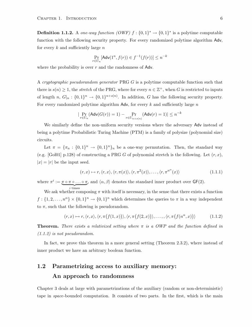
Let π = πn : 0, 1n → 0, 1nn be a one-way permutation. Then, the standard way
(e.g. [Gol01] p.128) of constructing a PRG G of polynomial stretch is the following. Let (r, x),
|x| = |r| be the input seed.
(r, x) 7→ r, 〈r, x〉, 〈r, π(x)〉, 〈r, π2(x)〉, . . . , 〈r, πnα(x)〉 (1.1.1)
where πi := π π . . . π︸ ︷︷ ︸i times
, and 〈α, β〉 denotes the standard inner product over GF(2).
We ask whether composing π with itself is necessary, in the sense that there exists a function
f : 1, 2, . . . , nα × 0, 1n → 0, 1n which determines the queries to π in a way independent
to π, such that the following is pseudorandom.
(r, x) 7→ r, 〈r, x〉, 〈r, π(f(1, x)
)〉, 〈r, π
(f(2, x)
)〉, . . . , , 〈r, π
(f(nα, x)
)〉 (1.1.2)
Theorem. There exists a relativized setting where π is a OWP and the function defined in
(1.1.2) is not pseudorandom.
In fact, we prove this theorem in a more general setting (Theorem 2.3.2), where instead of
inner product we have an arbitrary boolean function.
1.2 Parametrizing access to auxiliary memory:
An approach to randomness
Chapter 3 deals at large with parametrizations of the auxiliary (random or non-deterministic)
tape in space-bounded computation. It consists of two parts. In the first, which is the main
Chapter 1. Introduction 7
part, we initiate the study of a new approach to randomness in polynomial time computation
by quantifying the number of times random bits are accessed. Defining the concept is the main
contribution, and the technical developments relate this definition with previous questions in
efficient probabilistic computation. We stress that our interest in this definition is not about
the concept itself, but rather regarding its technical implications and potential. The second
part of Chapter 3 deals with variants of the model. Certain success in these variants serves as
indication that similar techniques may be applicable to our original model studied in the first
part. Furthermore, these variants are of independent interest. For example, using a simple
argument we make progress regarding the status of PolyLogSpace 6⊆ P, for which nothing was
known before.
Part of the content of Chapter 3 appears in [Pap09], and in joint work with David and
Sidiropoulos [DPS09b, DPS09a].
Randomness is central to computer science and its intersection with engineering, and nat-
ural sciences. Some of the most intriguing questions in Computational Complexity regard the
gap between polynomial time and its probabilistic analogs, e.g. RP, BPP. It is conjectured (e.g.
[IW97, KI04, NW88]) that this gap is small or even that randomness is in general not neces-
sary. Derandomizing probabilistic polynomial time (e.g. P = BPP) is a difficult mathematical
problem since it is ultimately related to proving superpolynomial circuit lower bounds [KI04].
Consider a randomized procedure performing a random walk in a graph. After each tran-
sition the algorithm “forgets” the random bits used so far. Contrast this with a randomized
procedure where random bits used at one step of the computation are revisited in future steps.
We aim for a definition which allows us to distinguish between these two scenarios. Our con-
tribution to the area is a new approach to quantifying restricted access to randomness during
arbitrary polynomial time (polytime) computation. Unlike previous approaches which quantify
the number of random bits, we parameterize the number of times the random tape is being
scanned. The intention is to formalize the concept of “use of randomness in polytime computa-
tion”. The way we formalize this intuition is somewhat debatable, given that such a definition
is not meaningful for a regular polytime bounded Turing Machine (TM). A TM equipped with
a read-only random tape in a single pass over the random tape can copy on its workspace all
the random bits it’s going to use. Hence, defining such a parametrization is a non-obvious task.
We apply a space-bounded characterization of polynomial time using Stack Machines (SMs)
due to Cook [Coo71] (Cook calls these machines Auxiliary PushDown Automata). Identifying
polynomial time as logspace computation equipped with unbounded recursion, is one of the
most intriguing, albeit nowadays non-central, concepts in Theoretical Computer Science. We
extend Stack Machines by adding a read-only, polynomially long random tape and we quantify
on the number of passes over the random tape. All Stack Machines have a read-only input
Chapter 1. Introduction 8
tape, and logarithmic worktape unless mentioned otherwise. We refer to a Stack Machine with
an auxiliary (e.g. random or non-deterministic) tape as a Verifier Stack Machine or vSM.
Definition 1.2.1. For a language L ⊆ 0, 1∗ we say that L ∈ RPdL[r] if there exists a vSM
M such that for every x ∈ 0, 1∗ it makes at most r(|x|) passes (i.e. it reverses r(|x|) − 1
times) over its polynomially long, read-only random tape, and if x ∈ L then M(x) accepts with
probability ≥ 12 , else if x 6∈ L then M(x) rejects with probability 1.
RPdL stands for Randomized Push-down Logspace. This abbreviation is chosen to empha-
size the relation with RP, since RPdL with an unbounded (or exponential - see e.g. [Ruz81])
number of passes is RP.
By changing the error condition to be two-sided we similarly define BPPdL[·] and PPdL[·],whereas if we consider one-sided unbounded error (equivalently: the external tape contains
non-deterministic bits) we define NPdL[·].We recall the definitions of probabilistic polynomial time e.g. RP, coRP,BPP in Chapter
3. For detailed definitions for probabilistic Turing Machines (PTMs), related classes, and
introductory treatment cf. [AB09].
On the naturalness of the definition. Our formalization of the “use of randomness” in
polynomial time computation goes through a space-bounded model. Thus, certain skepticism
arises whether this definition defines the concept in a natural way. Philosophy aside, the RPdL
hierarchy is introduced in order to be collapsed. The hope is that by changing the perspective
we may obtain additional technical insight towards showing P = BPP. Regardless of any
agreement or disagreement on its naturalness, from a technical perspective alone this definition
creates an exciting potential. It brings together tools developed in many excellent works in
Streaming, Communication Complexity, Derandomization, and Complexity Theory related to
Stack Machines (AuxPDAs).
Current stage of research - Motivating questions. At this stage we were not able to
derandomize BPP. We have obtained partial results which (i) provide connections of this new
concept to previously known concepts, and (ii) for variants of this model we obtain results
indicating possible future partial derandomization of RP or BPP, along with developments of
independent interest. Here is the list of the main questions motivating the technical develop-
ment.
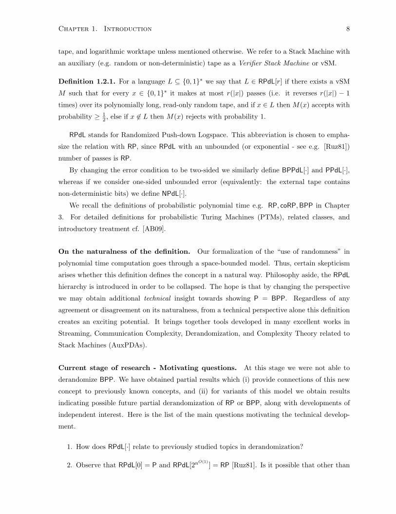
1. How does RPdL[·] relate to previously studied topics in derandomization?
2. Observe that RPdL[0] = P and RPdL[2nO(1)
] = RP [Ruz81]. Is it possible that other than
Chapter 1. Introduction 9
the coincidence for these two extremes, in the intermediate RPdL[r(n)] levels things don’t
behave smoothly as r(n) grows from 0 to 2nO(1)
?
3. Is there any indication that this approach may yield universal types of derandomization
that were previously unknown?
4. What can be said for variants of the model?
Questions (1) and (2) are addressed through the same technical results. Similarly, for
questions (3) and (4) every indication and success in derandomization, through our approach,
refers to variants of the model. In particular, we define similar hierarchies roughly between
NC1 and RNC1 (and BPNC1), and succeed in derandomizing the polylogarithmic range of this
hierarchy. Also, for other variants of the model we provide some results of independent interest.
1.2.1 Related work
Stack Machines. [Coo71] characterizes polytime computation in terms of Stack Machines
(AuxPDAs): logspace bounded TMs equipped with an unbounded stack. Recursive logspace
computation is a natural concept. Moreover, SMs exhibit quite interesting equivalences to
other models of computation. Our work relies on the connections between deterministic (and
nondeterministic) logspace and time-bounded SMs, and that of SAC (and NC) circuits with
various forms of uniformity [All89, BCD+89, Ruz80, Ruz81, Ven91]. When simultaneously to
the space, we also bound the time, there is a constructive and direct correspondence (which
intermediately goes through ATMs) between SMs and combinatorial circuits. This enable us to
blur the distinction between space-time bounded SMs and families of circuits. In a study of NC
in presence of strong uniformity (P-uniformity) [All89] studies SMs with restricted input-head
moves. This is related to the concept of head-reversals on the random tape considered in our
paper. For example, the discussion in [All89] (p.919) about the fact that the natural restriction
on the head-moves of a SM translates to something more subtle in case of ATMs, is related to
our definition of essential use of randomness using SMs with restricted number of scans on the
random tape.
Derandomization. There is a long line of research in derandomization. Successful stories
range from straightforward algorithms e.g. for MaxSAT (e.g. [AB09]) to quite sophisticated
ones such as the AKS primality test [AKS04]. There is a plethora of works that aim to de-
randomize probabilistic polynomial time using certain types of pseudorandom generators. The
majority of them relate the problem of derandomization to the problem of proving lower bounds
for the average-case complexity of one-way functions [Yao82], or to arbitrary hard functions (cf.
Chapter 1. Introduction 10
[NW88, IW97, STV99, Uma03]). The general theme of this research direction comes under the
title “randomness-hardness tradeoffs”. These works are in line with our intuition about the
circuit complexity of certain problems in E, EXP or NEXP. They provide evidence that deran-
domization of classes such as BPP might be possible, and simultaneously they give evidence
about the conceptual difficulty of achieving such a goal.
Accessing the random tape. To the best of our knowledge, prior to our work there are only
few other works asking similar questions. A corollary of [KV85] is PSPACE can be characterized
(with zero-error) with a logspace bounded TM with two-way access over an exponentially long
read-only random tape. The work closest to ours is [Nis93a]. Nisan shows that a logspace
TM with two-way access over a polynomially long random tape decides with zero-error the
languages decided by such machines where the error is 2-sided and the random tape is being
accessed once. In [Nis93a]’s notation BPL ⊆ ZP∗L.
1.2.2 Contribution
Definitions of complexity classes are given in Chapter 3. Our exposition is RP-centric; every-
thing holds for BPP, the 2-sided error case.
The main result of [Coo71] implies the first non-trivial derandomization of RPdL[1] = P (i.e.
a single pass over the randomness). In case of 2-sided error things are more complicated - we
show BPPdL[1] = P in Section 3.3.
The randomness complexity grows smoothly with the level of the hierarchy. We
relate the question of derandomizing along the RPdL hierarchy to the question of derandomizing
RNC. In particular, derandomization along the RPdL hierarchy implies derandomization of RNC.
More importantly a partial converse, modulo the derandomization technique, holds. That is, if
RNC is being derandomized using pseudorandom generators, then the same generators can be
used to derandomized RPdL.
Derandomizing a class believed to be strictly inside P, we derandomize a class which
contains P.
Technically, we proceed by introducing3 the model of Randomness Compilers, which is also of
independent interest. A randomness compiler M is a polytime transducer that given an input
x outputs a polysize circuit of depth polylogarithmic in n = |x|. Then, acceptance of x is being
determined by the acceptance probability of this circuit when it is evaluated on random inputs.
3This model was suggested by Mark Braverman who asked about its relation to probabilistic vSMs.
Chapter 1. Introduction 11
If for a language L, M outputs polysize circuits of constant fan-in and depth O(logi n) then we
say that L ∈ P+RNCi, where acceptance/rejection has one-sided error.
We remark that P+RNC is different from P-uniform RNC, since in P+RNC the circuit
depends on the input, not only on its length. In particular, P ⊆ P+RNC whereas the same is
believed not to be true if instead of P+RNC we had RNC.
Our main theorem (Theorem 3.2.3) relates the RPdL to the P+RNC hierarchy.
Theorem 3.2.3. Let i ∈ Z+. Then, P+RNCi ⊆ RPdL[2O(logi n)] ⊆ P+RNCi+1.
Remark 1.2.2. Consider the intuitive statement that polynomial size circuits of increasing depth
correspond to increasing complexity. The fact that we compile all the randomness we need in
such depth-growing polysize circuits (Theorem 3.2.3) makes precise the title “The randomness
complexity grows smoothly with the level of the hierarchy”.
A corollary of Theorem 3.2.3 is that to derandomize the quasipolynomially many (out of
exponential) levels of RPdL it suffices to construct PRGs secure against RNC circuits. These
PRGs are somewhat different from the cryptographic PRGs introduced earlier.
Definition 1.2.3 (PRGs against adversaries with fixed complexity bounds). Let 0 < ε < 1,
k ≥ 1. Let G : 0, 1∗ → 0, 1∗ be a function, such that G(z) is computable in time 2O(|z|1/k).
We say that G is an (NCi, k, ε)-pseudorandom generator if for every non-uniform NCi circuit-
family C and for sufficiently large |z| := n, z ∈ 0, 1∗, where |G(z)| = 2|z|1/k
:= m
|Prz∈R0,1n [Cm(G(z)) = 1]− Prρ∈Um [Cm(ρ) = 1] | ≤ ε
where Cm ∈ C has m input bits.
The precise technical statement follows.
Theorem 3.2.4. Let k, i ≥ 1. If there exists a (NCi+1, k, 17)-PRG, then RPdL[2O(logi n)] ⊆
DTIME(2O(logk n)).
Hence, if there exists a k for all i’s then RPdL[npolylogn] ⊆ DTIME(2O(logk n)), whereas if k
is a function of i then RPdL[npolylogn] ⊆ QuasiP, where RPdL[npolylogn] := ∪k>0RPdL[2logk n] and
QuasiP := ∪k>0DTIME(2logk n). We remark that a slightly different argument proves that it is
sufficient to assume that the PRG is secure against SACi circuits4, instead of NCi+1.
Variants of the model: concrete success stories. There are two kinds of variants of
probabilistic vSMs. One where the interpretation of the auxiliary tape changes; e.g. it contains
4A family of SACi circuits is a family of ACi circuits where the ∧ gates have bounded fan-in and all thenegations are to the input level.
Chapter 1. Introduction 12
non-deterministic bits. The second is where we get rid of the stack and instead we consider
usual logspace machines together with a parametrized auxiliary tape, henceforth called vTMs.
A vTM is a logspace bounded Turing Machine, equipped with a poly-long auxiliary tape on
which we count the number of head-reversals. The first kind of variant leads to results that are
conceptually of limited interest, so we will focus on vTMs. Among others, for vTMs we obtain
results that serve as an indication that concrete results are possible in their stack-equipped
counterpart.
The previous technical discussion (Theorems 3.2.3 and 3.2.4) on the derandomization of
P+RNC leaves out a detailed treatment for P+RNC1 using vSMs. In other words, it may
be possible to derandomize the first few levels of RPdL without the full derandomization of
RNC2. In fact, we conjecture that the first, say polylogarithmically many levels are possible to
derandomize without the need to resort to methods of much deeper theoretical understanding,
other than the one the current state of knowledge suggests. To that end a generalization of
classical space-bounded Nisan’s PRG may be of use. Here is a similar discussion for such a
derandomization for vTMs (i.e. machines without a stack).
Independent to our question, the derandomization of RNC1 and BPNC1 is by itself a major
open question. It is easy to see that the simulation of NC1 circuits by logspace machines, directly
extends to the simulation of BPNC1 circuits by probabilistic vTMs. Hence, to derandomize
BPNC1 it is sufficient to derandomize the computation of probabilistic vTMs. We make the
discussion BPNC1-centric, since for one-sided error using corollaries from Section 3.5.2 we can
obtain part of the results without relying on pseudorandom generators.
By parametrizing on the number of passes over the random tape of a vTM we define a
hierarchy of classes BPL[r(n)] (similar to BPPdL[r(n)]), where BPL[0] = LogSpace, BPL[1] =
BPL and BPL[poly] := ∪k>0BPL[nk] ⊇ BPNC1. Using a simple analysis of a more general
property of Nisan’s classical space PRG [Nis92] we obtain the following theorem. The same
result can be obtained from [INW94], using a more complicated PRG. However, the fact that
the original PRG of Nisan has the same property was not known before5.
Theorem 3.4.5. BPL[polylog] := ∪k>0BPL[logk n] ⊆ QuasiP.
We complement this result, by showing that the above statement roughly exhausts the
fooling power of Nisan’s PRG. That is, we provide a logspace distinguisher that breaks the
PRG with polynomially many passes, even for seeds of size 2c√
logn, for every c > 0.
Finally, we consider nondeterministic vTMs, i.e. logspace Turing Machines, with a poly-
nomially long, nondeterministic tape. We denote the corresponding class as NL[r(n)]. Our
study for these types of machines goes beyond the scope of derandomization, but it does fall
5Noam Nisan, personal communication.
Chapter 1. Introduction 13
into the same context of restricting access to the auxiliary tape. For the extreme r(n)’s we
have that NL[0] = LogSpace, NL[1] = NL, and NL[poly] = NP, since NP predicates can be
verified in logspace. We are interested in understanding the effect of restricted access to NP-
witnesses. We characterize the classes between NL and NP in a simple way that has several
theoretical and practical implications. The practical implications are related to SAT-solvers.
In particular, it is quite a coincidence that the class NL[w(n)logn ] has as a complete problem the
pathwidth-parametrized satisfiability problem of width w(n). The relevant definitions including
the definition of Exponential Time Hypothesis or ETH (see below) are given in Chapter 3. Here
are two consequences of our study.
It is well-known6 that PolyLogSpace 6= P, and the assumptions PolyLogSpace 6⊆ P and
P 6⊆ PolyLogSpace are very well-known due to their implications. However, it was fundamentally
unknown whether any known assumption implies e.g. PolyLogSpace 6⊆ P. Here is a simple
corollary of our study.
Theorem 3.5.8. PolyLogSpace ∩NP 6⊆ P, unless the ETH fails. Furthermore, under the same
assumption there exists a naturally defined L ∈ PolyLogSpace ∩ NP and L /∈ P.
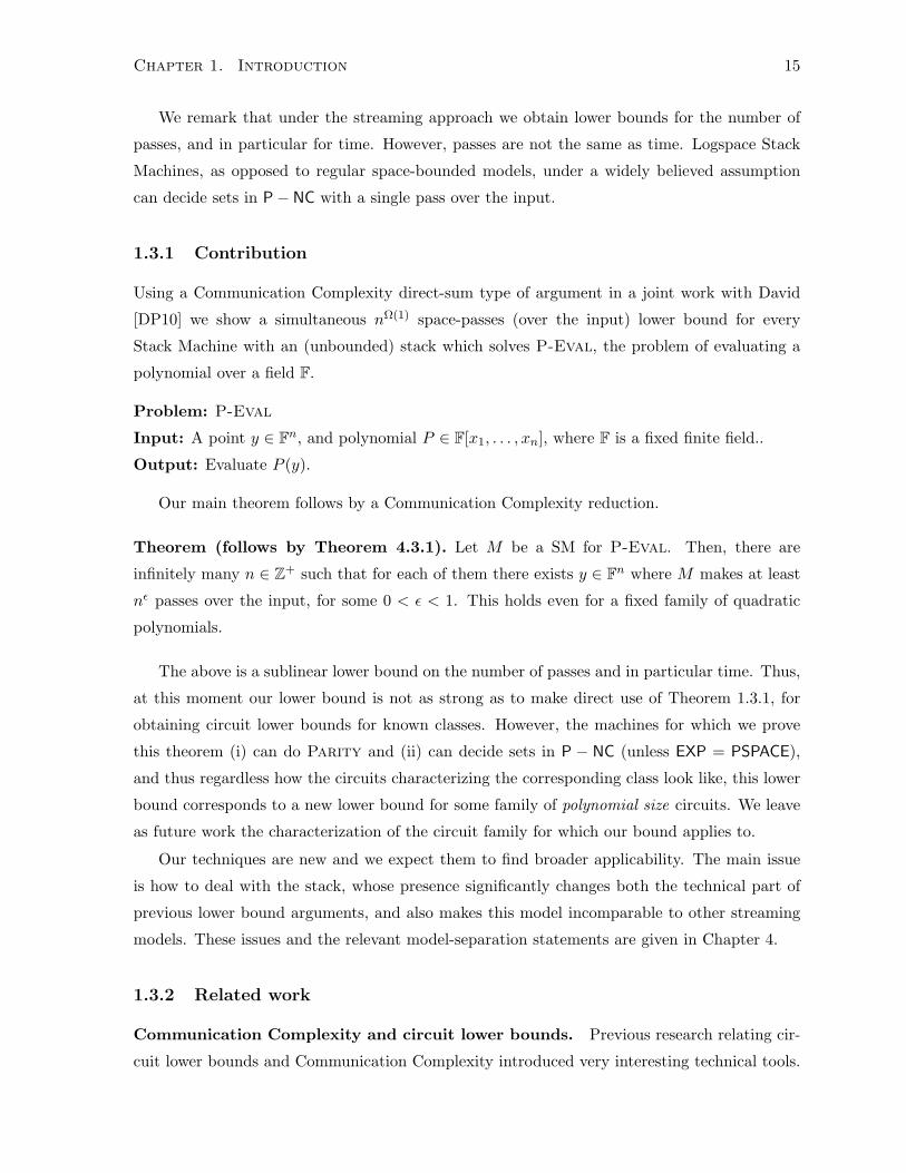
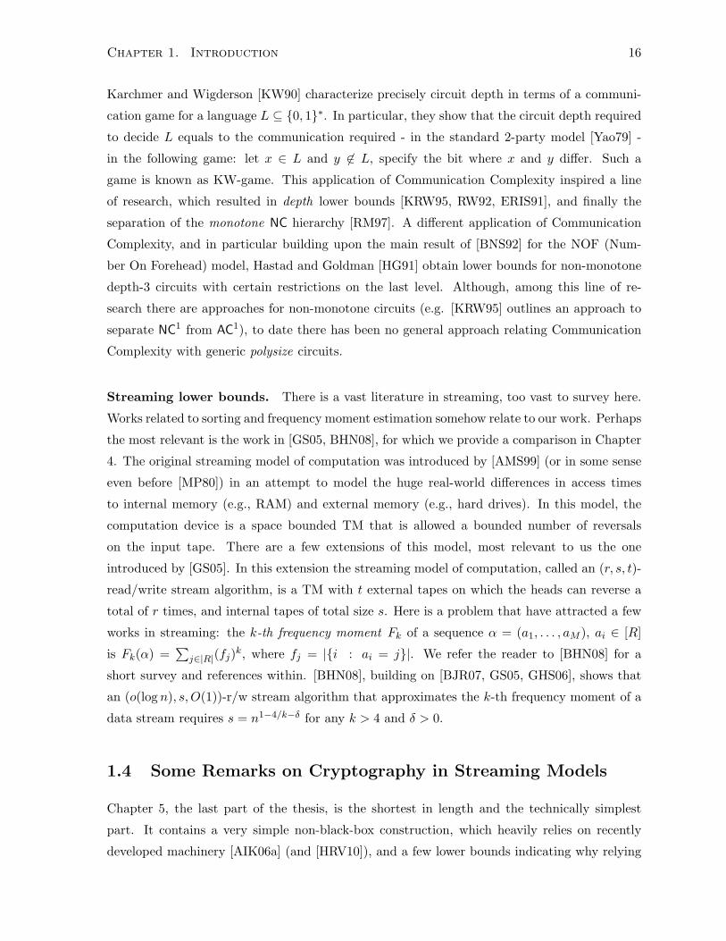
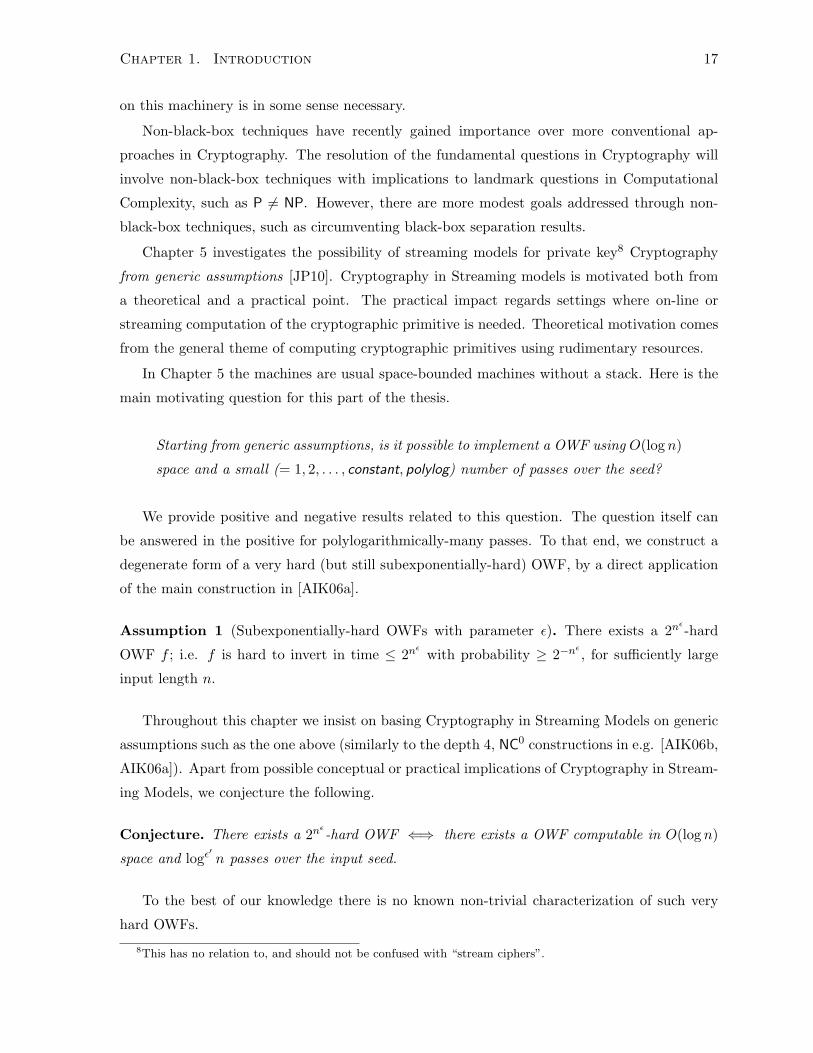
Under a further complexity assumption we show that the following diagram is correct. That
is, the classes NL[r(n)], intersect P properly, all the way to the limit where we simultaneously get
P and NP. For polylogarithmic r(n) this makes them natural, syntactically7 defined, classes
between P and NP (and incomparable to P) closed under logspace reductions, with natural
complete problems. In Chapter 5 we obtain an even stronger (and more complicated) result if
instead ETH we have standard cryptographic assumptions (under the current state of knowledge
incomparable to ETH).
1.3 An approach to lower bounds
Proving circuit lower bounds for efficiently computable problems is one of the main goals of
Computational Complexity. In Chapter 4 we outline a new framework to obtain memory-
access lower bounds for problems in P, and in particular for problems in the NC hierarchy, and
we make the first non-trivial technical steps. The novelty of our general framework is that
streaming lower bounds are translated to depth lower bounds for polynomial size circuits. We
do this by observing a relation between older works in Computational Complexity for Stack
Machines (AuxPDAs) and streaming on a space-bounded model with an unbounded stack. By
unbounded we mean that we do not charge passes for accessing the stack. It is not obvious why
6The space hierarchy theorem implies that PolyLogSpace does not have complete sets under logspace reduc-tions.
7Kaveh Ghasemloo made this observation.
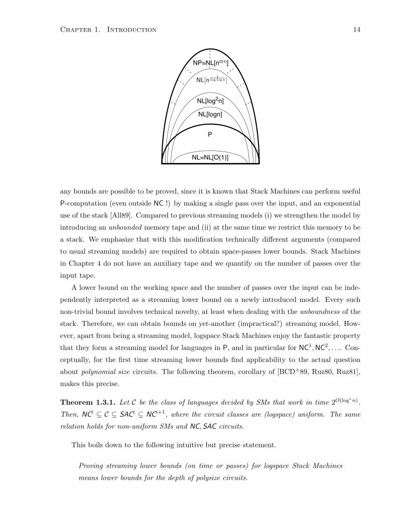
Chapter 1. Introduction 14
P
NL=NL[O(1)]
NL[logn]
NL[log2n]
NP=NL[nO(1)]
NL[n1
log log n ]
any bounds are possible to be proved, since it is known that Stack Machines can perform useful
P-computation (even outside NC !) by making a single pass over the input, and an exponential
use of the stack [All89]. Compared to previous streaming models (i) we strengthen the model by
introducing an unbounded memory tape and (ii) at the same time we restrict this memory to be
a stack. We emphasize that with this modification technically different arguments (compared
to usual streaming models) are required to obtain space-passes lower bounds. Stack Machines
in Chapter 4 do not have an auxiliary tape and we quantify on the number of passes over the
input tape.
A lower bound on the working space and the number of passes over the input can be inde-
pendently interpreted as a streaming lower bound on a newly introduced model. Every such
non-trivial bound involves technical novelty, at least when dealing with the unboundness of the
stack. Therefore, we can obtain bounds on yet-another (impractical?) streaming model. How-
ever, apart from being a streaming model, logspace Stack Machines enjoy the fantastic property
that they form a streaming model for languages in P, and in particular for NC1,NC2, . . .. Con-
ceptually, for the first time streaming lower bounds find applicability to the actual question
about polynomial size circuits. The following theorem, corollary of [BCD+89, Ruz80, Ruz81],
makes this precise.
Theorem 1.3.1. Let C be the class of languages decided by SMs that work in time 2O(logi n).
Then, NCi ⊆ C ⊆ SACi ⊆ NCi+1, where the circuit classes are (logspace) uniform. The same
relation holds for non-uniform SMs and NC,SAC circuits.
This boils down to the following intuitive but precise statement.
Proving streaming lower bounds (on time or passes) for logspace Stack Machines
means lower bounds for the depth of polysize circuits.
Chapter 1. Introduction 15
We remark that under the streaming approach we obtain lower bounds for the number of
passes, and in particular for time. However, passes are not the same as time. Logspace Stack
Machines, as opposed to regular space-bounded models, under a widely believed assumption
can decide sets in P− NC with a single pass over the input.
1.3.1 Contribution
Using a Communication Complexity direct-sum type of argument in a joint work with David
[DP10] we show a simultaneous nΩ(1) space-passes (over the input) lower bound for every
Stack Machine with an (unbounded) stack which solves P-Eval, the problem of evaluating a
polynomial over a field F.
Problem: P-Eval
Input: A point y ∈ Fn, and polynomial P ∈ F[x1, . . . , xn], where F is a fixed finite field..
Output: Evaluate P (y).
Our main theorem follows by a Communication Complexity reduction.
Theorem (follows by Theorem 4.3.1). Let M be a SM for P-Eval. Then, there are
infinitely many n ∈ Z+ such that for each of them there exists y ∈ Fn where M makes at least
nε passes over the input, for some 0 < ε < 1. This holds even for a fixed family of quadratic
polynomials.
The above is a sublinear lower bound on the number of passes and in particular time. Thus,
at this moment our lower bound is not as strong as to make direct use of Theorem 1.3.1, for
obtaining circuit lower bounds for known classes. However, the machines for which we prove
this theorem (i) can do Parity and (ii) can decide sets in P − NC (unless EXP = PSPACE),
and thus regardless how the circuits characterizing the corresponding class look like, this lower
bound corresponds to a new lower bound for some family of polynomial size circuits. We leave
as future work the characterization of the circuit family for which our bound applies to.
Our techniques are new and we expect them to find broader applicability. The main issue
is how to deal with the stack, whose presence significantly changes both the technical part of
previous lower bound arguments, and also makes this model incomparable to other streaming
models. These issues and the relevant model-separation statements are given in Chapter 4.
1.3.2 Related work
Communication Complexity and circuit lower bounds. Previous research relating cir-
cuit lower bounds and Communication Complexity introduced very interesting technical tools.
Chapter 1. Introduction 16
Karchmer and Wigderson [KW90] characterize precisely circuit depth in terms of a communi-
cation game for a language L ⊆ 0, 1∗. In particular, they show that the circuit depth required
to decide L equals to the communication required - in the standard 2-party model [Yao79] -
in the following game: let x ∈ L and y 6∈ L, specify the bit where x and y differ. Such a
game is known as KW-game. This application of Communication Complexity inspired a line
of research, which resulted in depth lower bounds [KRW95, RW92, ERIS91], and finally the
separation of the monotone NC hierarchy [RM97]. A different application of Communication
Complexity, and in particular building upon the main result of [BNS92] for the NOF (Num-
ber On Forehead) model, Hastad and Goldman [HG91] obtain lower bounds for non-monotone
depth-3 circuits with certain restrictions on the last level. Although, among this line of re-
search there are approaches for non-monotone circuits (e.g. [KRW95] outlines an approach to
separate NC1 from AC1), to date there has been no general approach relating Communication
Complexity with generic polysize circuits.
Streaming lower bounds. There is a vast literature in streaming, too vast to survey here.
Works related to sorting and frequency moment estimation somehow relate to our work. Perhaps
the most relevant is the work in [GS05, BHN08], for which we provide a comparison in Chapter
4. The original streaming model of computation was introduced by [AMS99] (or in some sense
even before [MP80]) in an attempt to model the huge real-world differences in access times
to internal memory (e.g., RAM) and external memory (e.g., hard drives). In this model, the
computation device is a space bounded TM that is allowed a bounded number of reversals
on the input tape. There are a few extensions of this model, most relevant to us the one
introduced by [GS05]. In this extension the streaming model of computation, called an (r, s, t)-
read/write stream algorithm, is a TM with t external tapes on which the heads can reverse a
total of r times, and internal tapes of total size s. Here is a problem that have attracted a few
works in streaming: the k-th frequency moment Fk of a sequence α = (a1, . . . , aM ), ai ∈ [R]
is Fk(α) =∑
j∈|R|(fj)k, where fj = |i : ai = j|. We refer the reader to [BHN08] for a
short survey and references within. [BHN08], building on [BJR07, GS05, GHS06], shows that
an (o(log n), s, O(1))-r/w stream algorithm that approximates the k-th frequency moment of a
data stream requires s = n1−4/k−δ for any k > 4 and δ > 0.
1.4 Some Remarks on Cryptography in Streaming Models
Chapter 5, the last part of the thesis, is the shortest in length and the technically simplest
part. It contains a very simple non-black-box construction, which heavily relies on recently
developed machinery [AIK06a] (and [HRV10]), and a few lower bounds indicating why relying
Chapter 1. Introduction 17
on this machinery is in some sense necessary.
Non-black-box techniques have recently gained importance over more conventional ap-
proaches in Cryptography. The resolution of the fundamental questions in Cryptography will
involve non-black-box techniques with implications to landmark questions in Computational
Complexity, such as P 6= NP. However, there are more modest goals addressed through non-
black-box techniques, such as circumventing black-box separation results.
Chapter 5 investigates the possibility of streaming models for private key8 Cryptography
from generic assumptions [JP10]. Cryptography in Streaming models is motivated both from
a theoretical and a practical point. The practical impact regards settings where on-line or
streaming computation of the cryptographic primitive is needed. Theoretical motivation comes
from the general theme of computing cryptographic primitives using rudimentary resources.
In Chapter 5 the machines are usual space-bounded machines without a stack. Here is the
main motivating question for this part of the thesis.
Starting from generic assumptions, is it possible to implement a OWF using O(log n)
space and a small (= 1, 2, . . . , constant, polylog) number of passes over the seed?
We provide positive and negative results related to this question. The question itself can
be answered in the positive for polylogarithmically-many passes. To that end, we construct a
degenerate form of a very hard (but still subexponentially-hard) OWF, by a direct application
of the main construction in [AIK06a].
Assumption 1 (Subexponentially-hard OWFs with parameter ε). There exists a 2nε-hard
OWF f ; i.e. f is hard to invert in time ≤ 2nε
with probability ≥ 2−nε, for sufficiently large
input length n.
Throughout this chapter we insist on basing Cryptography in Streaming Models on generic
assumptions such as the one above (similarly to the depth 4, NC0 constructions in e.g. [AIK06b,
AIK06a]). Apart from possible conceptual or practical implications of Cryptography in Stream-
ing Models, we conjecture the following.
Conjecture. There exists a 2nε-hard OWF ⇐⇒ there exists a OWF computable in O(log n)
space and logε′n passes over the input seed.
To the best of our knowledge there is no known non-trivial characterization of such very
hard OWFs.
8This has no relation to, and should not be confused with “stream ciphers”.
Chapter 1. Introduction 18
1.4.1 Contribution
Under a widely believed cryptographic assumption, we can easily establish the ⇒ direction of
this conjecture.
Theorem 5.2.3. Suppose that there exists a 2nΩ(1)
-hard OWF, and a OWF computable in
logspace (and no restriction on the number of passes over the input seed). Then, there exists a
OWF computable in O(log n) space and logO(1) n many passes over the input seed.
The existence of a OWF in logspace (with unbounded many passes over the input) is a very
mild cryptographic assumption (see below on related work).
Note that the O(log n) space bound is essential for appreciating the issue. For example,
consider a space bound ω(log n) and a sufficiently hard OWF. Then, it is easy to see (Example
5.1.1) why there exists a OWF computable with a single pass over the input. The same is not
true when the worktape becomes O(log n) small, even for arbitrary number of passes over the
input. In fact, it is counter-intuitive why it is at all possible.
Also, we show a number of (unconditional) negative results illustrating possible obstacles for
logspace streaming computation of a OWF. Using the last part of Chapter 3 we unconditionally
obtain that no OWF computable with O(1) many passes exists. Furthermore, we systematically
study the necessity of a non-black-box construction of such a OWF. In particular, we show that
natural implementations of popular, concrete intractability assumptions based on the hardness
of Factoring and Subset-Sum unconditionally require nΩ(1) space and passes to compute.
Then, we consider a possible black-box use of the NC0 OWFs constructed in [AIK06b]. We
show that NC0 circuits (with multiple outputs) cannot, in general, be simulated by logspace
transducers with a small number of passes. Finally, we show that there is no general simulation
of an ω(log n) space bounded transducer with a small number of passes over the input, by a
O(log n) model with an at most polynomial overhead overhead in the number of passes over
the input seed.
1.4.2 Related work
Streaming Cryptography falls into the general theme of computing cryptographic primitives
using rudimentary resources, and dates back at least 20 years. The existence of PRGs in
logspace (with an unbounded number of passes over the seed), or even AC0 or TC0, follows from
standard intractability assumptions on the hardness of Subset-Sum, Factoring, Discrete-
Log or lattice problems; e.g. [IN89, GL89, BM84, HILL99]. Regarding streaming constructions,
where the number of passes over the input seed is bounded, Kharitonov et al [KGY89] study
the possibility of such constructions, and they observe that ω(log n) space is sufficient. For
space O(log n), their main result is that no PRG of linear stretch exists when the input seed is
Chapter 1. Introduction 19
read a constant number of times. We improve on their main result by showing that no OWF
(and in particular no PRG that stretches n bits to n+ 1) exists. Up until our work, for space
O(log n), the literature deals only with impossibility results. Yu and Yung [YY94] show several
lower bounds for types of automata and machines that work in sub-logarithmic space. For the
next 15 years “rudimentary” means polynomial size circuits of constant depth and this line of
work gives possibility results and lower bounds.
The major breakthrough regards the construction of OWFs and PRGs (and other primitives)
in NC0 and in particular for circuits of depth 3 and 4; note that Cryan and Miltersen[CM01]
observe, based on the easiness of 2-SAT, that no PRG exists in NC0 of depth 2. The seminal
work of Applebaum, Ishai, and Kushilevitz [AIK06b, AIK06a, AIK08, AIK07] builds upon the
work of Randomizing Polynomials e.g. [IK00], and shows the possibility of Cryptography in
NC0: given a “cryptographic function” f construct a randomized encoding of f , which is a
distribution f that (i) preserves the security of f , and (ii) is much simpler to compute than
f . In particular, starting from the generic assumption that “cryptographic” functions can be
computed in logspace, the authors show how to construct a family of NC0 circuits by appropri-
ately compiling the corresponding polynomial size branching program. This amazing technical
achievement brings the combinatorics of cryptographic functions to a simplified setting, and
opens the possibility of better understanding cryptographic primitives. Our logspace streaming
construction depends on the specifics of this work. We remark that our construction relies
on circuits where every subcircuit is of small expansion. Goldreich [Gol00] proposes a OWF
computable by NC0 circuits of high expansion, and Bogdanov and Qiao [BQ09] compromise the
security of this function for certain values of the parameters. Very recently, [HRV10] gives a
highly parallel (and non-adaptive) construction of a PRG from an arbitrary OWF. In particular,
this can be used to improve the [AIK06a] result by weakening a cryptographic assumption.
Chapter 2
Black-box separations in
Cryptography
We answer in the negative two questions, one in Public-Key and one in Private-Key Cryptog-
raphy. The first is whether we can base Identity Based Encryption (IBE) in a black-box setting
on the existence of Trapdoor Permutations (TDPs) or on the average-case hardness of Deci-
sional Diffie-Hellman (DDH). The second asks whether it is possible to base in a black-box and
non-adaptive way the existence of pseudorandom generators (PRGs) on one-way permutations
(OWPs).
For intuition, motivation, and preliminary definitions see Section 1.1. In Section 2.1 we show
the impossibility of basing IBE on TDPs. The impossibility of IBE based on DDH is still work
in progress. In Section 2.2 we define and discuss the relativized setting for the DDH separation,
and we show that the security of a general IBE in this setting can be reduced to a restricted
type of IBE. This is a central technical difference with the separation in Section 2.1. In Section
2.3 we show that it is not possible to construct in a black-box way PRGs of super-linear stretch,
by making non-adaptive use of a one-way permutation (OWP). This black-box separation is
conceptually related to Cryptography in Streaming Models (Chapter 5).
2.1 Black-box separation of IBE from TDPs
We ask whether a secure IBE can be built from the weaker primitive of TDPs using a black-box
construction and without any further assumptions. We aim for a strong type of impossibility
result. As such the question is whether we can construct a semantically secure IBE system
for encrypting a single bit message. Here, we use a weakened version of IBE semantic security
defined in [BF03]. In our definition the adversary non-adaptively requests private keys of
identities of its choice even before seeing the public parameters, and then tries to break semantic
20
Chapter 2. Black-box separations in Cryptography 21
security for some other identity.
Our separation proof builds a natural oracle O relative to which TDPs exist. We then
show that all candidate WSS-IBE systems (SetupO,KeygenO,EncO,DecO) are insecure against
a polynomial time adversary A with access to O and to a PSPACE oracle. The oracle O is very
natural and directly implies the existence of trapdoor permutations. The difficult part of the
proof is constructing the adversary Adv that breaks any given candidate SS-IBE system relative
to this oracle.
Our proof brings to light the essential property of IBE systems: an IBE system creates an
exponential number of public keys (identities) and compresses all of them into a short string
called the public parameters. This ability to represent exponentially many public keys using a
short string is not possible with a TDP. This exponential compression is achieved in existing
IBE constructions using algebraic properties (see also Section 2.2) for further discussion.
For motivation and discussion see Section 1.1. In Section 2.1.1 we fix our notation, and
define what is a Weakly Semantically Secure IBE (WSS-IBE) in the TDP Model. In Section
2.1.2 we state the black-box separation theorem and discuss its trivial direction, i.e. that in
our oracle model TDPs exist. In Section 2.1.3 we state our main theorem and we describe
the attack algorithm Adv. In Section 2.1.4 we give an outline of the proof, and Section 2.1.5
contains the details of the argument.
2.1.1 Definition of Weakly Semantically Secure IBE in the TDP Model
Recall that an IBE system consists of four deterministic algorithms [Sha85, BF01] (Setup,Keygen,Enc,Dec).
In our case an IBE system also specifies constants λ, q, n ∈ Z+, and ε ∈ (1/2, 1] as part of its
description, an the algorithms have access to the oracles g, e, d described in Section 1.1 and is
parameterized by λ. The IBE algorithms are allowed to make at most q queries to their oracle
during a single execution. The parameter n is used to determine the number of random bits
and the output lengths of the IBE algorithms. The parameter ε specifies the IBE’s level of
correctness, that is, a ciphertext generated from the correct distribution will be successfully
decrypted with probability ≥ ε.The functionality of each algorithm is as follows: algorithm Setup(MSK) takes as input
a master secret key MSK ∈ 0, 1n; it outputs public parameters PP ∈ 0, 1n. Algorithm
Keygen(MSK, ID) is deterministic, and it takes as input the master secret key MSK, and an
identity ID ∈ 0, 1n. It outputs the private key SKID ∈ 0, 1n for identity ID. The encryption
algorithm Enc(PP, ID, b, r) encrypts a bit b for a given identity ID using public parameters PP
and randomness r ∈ 0, 1n; it outputs a ciphertext C ∈ 0, 1n. The decryption algorithm
Dec(SKID, C) decrypts a ciphertext C using the private key SKID and is deterministic. Note
that making the algorithm Keygen deterministic does not restrict the type of IBE constructions
Chapter 2. Black-box separations in Cryptography 22
that our results cover since any secure IBE with a randomized Keygen can be converted into
a secure IBE with a deterministic K by applying a pseudo-random function to the identity in
order to obtain (pseudo) random bits for Keygen.
An IBE system must satisfy the following correctness property: for every ID ∈ 0, 1n,
b ∈ 0, 1
Pr
[PP← Setup(MSK), SKID ← Keygen(MSK, ID),
C ← Enc(PP, ID, b); Dec(SKID, C) = b
]≥ ε
Normal Form. We restrict our attention (without loss of generality) to IBEs that satisfy
the following condition: each oracle query of the form d(sk, ·) must be followed by the query
g(sk). We use this condition to avoid situations in which we know a trapdoor for some unknown
trapdoor permutation.
Definition of Security. For security we use a weakened version of the IBE semantic security
that is defined in [BF03]. The weak semantic security is defined using a game in which the
attacker starts by choosing a polynomially long sequence of identities for which it wishes to
obtain private keys, along with the challenge identity that it is going to try and break. This
is done even before the adversary is given the public parameters. The adversary is then given
the public parameters, a sequence of private keys for the above identities (except the challenge
identity), and an encryption of a random bit for the challenge identity using the public param-
eters. More precisely, weak semantic IBE security is defined using a game between a challenger
and an adversary Adv in which both parties are given a security parameter λ is input. The
game proceeds as follows:
Setup: The adversary submits a challenge identity ID∗, and a sequence of identities
ID1, . . . , IDl where l = l(q) and l(·) is some polynomial.
Private Keys: The challenger chooses at random MSK ∈ 0, 1n. It then computes
PP ← Setup(MSK), and SKi ← Keygen(1λ,MSK, IDi) for 1 ≤ i ≤ l. The tuple
(PP,SK1, . . . ,SKl) is given to the adversary.
Challenge: The challenger chooses at random r ∈ 0, 1n, b ∈ 0, 1. It then computes
C∗ ← Enc(PP, ID, b; r), and C∗ is given to the adversary.
Guess: The adversary outputs a guess b′ ∈ 0, 1, and wins if b′ = b.
We define the advantage of the adversary Adv in attacking the scheme E as
AdvantageE,Adv :=∣∣∣∣Pr[b = b′]− 1
2
∣∣∣∣The probability is over the random bits used by the challenger and the adversary.
Chapter 2. Black-box separations in Cryptography 23
2.1.2 The black-box separation Theorem
In the language of [RTV04] we show that there is no fully black-box reduction of the security of
a TDP to a WSS-IBE. We do this by showing that in the relativized setting we defined above,
TDPs exist (a.c. for a randomly chosen O), and at the same time there exists an adversary that
breaks the security of every (even the weakly semantically secure) IBE with access to O. The
first claim is immediate by the definition of the oracle setting. The other part is technically
involved.
Claim 2.1.1. There exists a trapdoor permutation scheme such that for all oracle adversary’s
A that make at most a polynomial number of queries to the oracle O we have that for sufficiently
large λ the adversary’s success in breaking the trapdoor permutation is negligible in λ, where λ
is the security parameter of the scheme.
Our main theorem proves something slightly more general than what mentioned above, since
our attack is successful even against reasonably incorrect IBEs; i.e. as close to the correctness
guarantee ε as we wish. Here is the main theorem.
Theorem 2.1.2. Let q ∈ Z+, and ε ∈ (1/2, 1]. Then, for every IBE which makes at most
q queries to the oracle, and has correctness parameter ≥ ε, and for every 1/2 < δ < ε there
exists an adversary Adv and constant c > 0 such that Adv makes at most qc oracle queries and
decrypts the challenge ciphertext successfully with probability ≥ δ.
2.1.3 The attack algorithm
In this section we describe an attack algorithm that breaks every IBE in the trapdoor permu-
tation model. Our attack requires only a polynomial number of queries to the oracles, and can
be implemented in polynomial time if we add a PSPACE oracle. We start with a high level
overview of the attack.
The algorithm Setup in an IBE takes a random private MSK and outputs a public key
PP. During its computation Setup may make use of its trapdoor permutation oracles, and use
the results of the queries to construct the final public key. In our model any Setup algorithm
that aims to be secure will have to make “essential” use of its oracles. Otherwise, an adversary
could simply invert the function computed by Setup, thus obtaining a valid private key. Looking
ahead to our analysis, we show that Setup has to make use of the trapdoor generation oracle
Setup by generating several public keys of trapdoor permutations, and embedding them in
the public parameters of the IBE. After the IBE public parameters are fixed the algorithm
Keygen may include in each individual private key of an identity one or more trapdoors for the
permutation public keys that were embedded in the IBE public parameters. We argue that
Chapter 2. Black-box separations in Cryptography 24
using the permutation public keys that are embedded in the IBE public parameters is the only
way to encrypt securely. Thus, if the adversary could collect all the important1 trapdoors for
the embedded public keys it would be able to decrypt any ciphertext.
It is precisely this task of discovering the important trapdoors that is made possible due
to the fact that the public parameters of an IBE encode an exponential number of public
keys, and at the same time contain only a polynomial number of embedded permutation public
keys. Suppose that a certain permutation, for which the public key is embedded in the public
parameters, is used in a significant way to encrypt a bit to some identity. Then, for the
decryption to work the corresponding trapdoor must be embedded in that identity’s private
key. Thus, if there are q permutation public keys embedded in the public parameters there
can be at most q identities for which the identity’s private key contains a trapdoor for one of
the trapdoor permutations that are embedded in the public parameters. Thus, for every set of
identities that is significantly bigger than q only a small portion of the identities have private
keys that reveal new important trapdoors. This immediately yields the following approach for
an attack: let S be a sufficiently large set of identities (say of size qc). We select a challenge
identity at random from S and ask to see the private keys for all the other identities in S. With
probability 1 − 1/qc−1 the private keys that we obtained contain all the important trapdoors
that are needed to decrypt ciphertexts that were addressed to any identity in S, including the
challenge identity.
While the above argument gives an intuitive sketch for an attack algorithm, the actual
algorithm and proof contain several challenging subtleties. The most interesting challenges
arise from the fact that the public parameters and IBE private keys may be encoded in an
arbitrary manner. In particular, an attack algorithm that simply “looks” at an IBE private key
will not necessarily be able to tell which oracle secret keys are embedded in it. We resolve this
issue by encrypting a random bit to that identity, and then decrypting the resulting ciphertext.
We record all trapdoors that are actually used in queries to the permutation inverse oracle d
during the computation of the encryption and decryption algorithms.
The fact that we discover important trapdoors by observing a sample computation of the
encryption and decryption algorithms for each identity leads to the main technical complication
in our attack. Since we discover only trapdoors that are used in the decryption of one ciphertext
for each identity, it is crucial that all the values that appear during the decryption of the
challenge ciphertext are distributed in a manner as they would be if the correct private key
and the actual oracle were used for the decryption. Otherwise, if the decryption process for the
1Some trapdoor public keys may be generated by Setup and embedded in PP but never used by the encryptionalgorithm. For these public keys there may be no way of recovering the trapdoors with a small number of queries.However, it is also unnecessary as the adversary will never need these trapdoors to decrypt.
Chapter 2. Black-box separations in Cryptography 25
challenge identity looks significantly different from the decryption for the other identities then
new trapdoors may be required to decrypt the challenge ciphertext.
Partial oracles. Our attack algorithm will generate during its computation trapdoor permu-
tation oracles that are defined only on a subset of the possible inputs. We call such functions
partial trapdoor permutation oracles. The following definition describes when such a partial
oracle is extendable to a full oracle:
Definition 2.1.3. Let O′ = (g′, e′, d′) be a function which is defined on part of the domain of
trapdoor permutation oracles. O′ is called a consistent partial oracle if it has all the following
properties:
(i) For every pk ∈ 0, 1λ, e′(pk, ·) is 1-1; (ii) for every sk ∈ 0, 1λ, d′(sk, ·) is 1-1; (iii)
for every sk such that g′(sk) is defined let pk = g′(sk). We require that for every x ∈ 0, 1λ,
e′(pk, x) = α is defined if and only if d′(sk, α) = x is defined.
The Attack Algorithm
For notational simplicity we will occasionally refer to the algorithm without using the O super-
scripts.
Let 1/2 < δ < ε ≤ 1, and q, n ∈ Z+. We now describe the attack algorithm Adv, which
plays the Identity-Based Encryption security game with a challenger C for a given IBE system
IBE = (Setup,Keygen,Enc,Dec) which makes at most q queries, has inputs of length n, and
has correctness guarantee ≥ ε. Adv wins with probability ≥ δ.The adversary starts by choosing five constants c1, c2, c3, c4, c5 such that c4 ≥ c1 + 2 and
2qc3−c1−1
+3
eqc2−c4+
2qc1−1
+10
qc5−(c1+c2+c3+c4+2)≤ ε− δ
2
Degenerate case
Our general adversary does not deal well with the following IBEs due to the small size of the
probability spaces in question, therefore, we break such IBEs separately.
If 2λ ≤ qc5 then the adversary proceeds as follows:
1. The adversary queries the oracles g, e, d on all 2λ inputs. After this step the adversary has
completely learned the oracle O. Thus, from this point on the adversary will not make
any additional oracle queries.
2. The adversary then chooses an arbitrary challenge identity ID∗ = 0 and asks to obtain an
encryption C∗ of a random bit to ID∗.
Chapter 2. Black-box separations in Cryptography 26
3. The adversary chooses MSK′ such that SetupO(MSK′) = PP, and computes SK∗ =
KeygenO(MSK′, ID∗).
4. Finally, the adversary computes and outputs DecO(SK∗, C∗).
Clearly in the degenerate case the adversary successfully decrypts the ciphertext with proba-
bility ε.
The general case
If 2λ > qc5 our adversary performs the following steps.
Initialization. The adversary starts by initializing a table L, which will be used to store
information that the adversary learns about the oracle O. More precisely, L is a set of tuples
of the form (α, β) where α specifies an oracle from g, e, d and the query to that oracle, and
β is the reply that was given to that query.
From this point on, every query that the adversary makes to the oracle O, and the answer
to that query are recorded in L.
Setup. Let S ⊆ 0, 1∗ be the set containing the binary encodings of the integers 1, . . . , qc1 .
The adversary picks uniformly at random ID∗ ∈R S, submits ID∗ as the challenge identity and
requests to see private keys for all ID 6= ID∗, ID ∈ S.
Challenge. The adversary is given a tuple (PP, SK1, . . . ,SKID∗−1, SKID∗+1, . . . ,SKqc1 , C∗).
From now on the adversary will make use of the public parameters PP and the private keys
SKi, but the challenge ciphertext C∗ will only be used in the last stage of the attack.
Step 1: Discovering important trapdoors. For each ID 6= ID∗, ID ∈ S, the adver-
sary chooses at random r ∈R 0, 1n, b ∈R 0, 1. Then, the adversary simulates C ←EncO(PP, ID, b; r) and DecO(SKID, C). Notice that during this step the adversary will add
to L, among other things, mappings of the form g(sk) = pk. Whenever such a mapping is
added to L we can invert the permutation pk successfully.
Step 2: Discovering frequent queries. The adversary repeats the following qc2 times:
chooses at random r ∈R 0, 1n, b ∈R 0, 1, and computes EncO(PP, ID∗, b; r).
Step 3: Discovering secret queries and decrypting the challenge. The adversary
chooses at random 1 ≤ k ≤ qc3 and repeats the following k times.
1. (Offline phase) The adversary chooses uniformly at random a global secret key MSK′,
and a partial oracle O′ = (g′, e′, d′) that satisfies the following properties: O′ \ L is of
Chapter 2. Black-box separations in Cryptography 27
size2 at most qc4 ; L ⊆ O′, that is, O′ contains the partial information that the adversary
has learned about O; GO′(MSK′) = PP; For every ID 6= ID∗, ID ∈ S it holds that
KeygenO′(MSK′, ID) = SKID; and KeygenO
′(MSK′, ID∗) is defined3.
We also require that O′ is a consistent partial oracle according to Definition 2.1.3.
2. Using the partial oracle O′ the adversary computes SK′∗ ← KeygenO′(MSK′, ID∗).
3. (Online phase) The adversary chooses at random r ∈R 0, 1n, b ∈R 0, 1, and com-
putes C ← EncO(PP, ID∗, b; r). Notice that here we are using the actual oracle O.
4. The adversary combines the partial oracle O′ and the actual oracle O into a new oracle
O′′. The precise description of O′′ is given in the next paragraph. The adversary then
simulates DecO′′(SK′∗, C). To decrypt the challenge ciphertext the adversary replaces C
with C∗ at the last repetition of this step. That is, at repetition k the adversary simulates
DecO′′(SK′∗, C∗) and obtains a bit b′.
Guess. The adversary outputs the bit b′ obtained in the last repetition of the previous stage.
The oracle O′′
The oracle O′′ is constructed by the adversary to create a single oracle which combines the
offline generated values of O′ with the actual oracle O. Note that we cannot avoid using the
oracle O in the decryption since it was used to encrypt the challenge ciphertext.
To describe O′′ we need to treat specially a certain type of permutations. We call trapdoor
permutations that are generated by Keygen for some ID, but not by Setup, “internal trapdoor
permutation”. Intuitively, the internal permutations are not accessible to the encryptor and
therefore we do not have to use the actual oracle to answer queries about them. Formally,
Definition 2.1.4. Let O′ be a partial oracle, and MSK′ ∈ 0, 1n. We define
(i) U to be the set of pk such that g(sk) is asked during SetupO′(MSK′) and received answer
pk.
(ii) V be the set of pk such that g(sk) is asked during KeygenO′(MSK′, ID)
for some ID ∈ S and received answer pk.
(iii) Lg be the set of pk such that there exists a mapping of the form4 [g(·) = pk] in L.
The set of internal trapdoor permutations is W = V \ U .
2That is, the number of mappings that were invented by the adversary, and did not appear in L, is at mostqc4 .
3By defined we mean that when Keygen is run on global secret key MSK′, O′ is sufficient to answer all ofKeygen’s queries. Note that c4 is large enough to allow O′ to contain all the offline values that are needed tosatisfy this condition.
4We write [g(·) = pk] ∈ L to denote that there exists an sk such that [g(sk) = pk] ∈ L.
Chapter 2. Black-box separations in Cryptography 28
The oracle. The oracle O′′ works on a query α as follows:
1. If O′(α) is defined then reply with O′(α).
2. Else If α is a query of the form e(pk, ·) (or d(sk, ·)) where pk ∈W \Lg (or there exists pk ∈W \Lg such that [g(sk) = pk] ∈ O′) then O′′ generates the answer randomly and records
it in O′. More precisely, if α is of the form e′′(pk, x) where pk is an internal trapdoor
permutation, or of the form d′′(sk, α) where g′(sk) is an internal trapdoor permutation,
then O′′ emulates a random permutation independent of the actual oracle O. Namely,
it responds randomly (and consistently), ensuring that e′′(pk, ·) is a permutation and
d′′(sk, ·) is its inverse, where g′(sk) = pk. By consistently we mean that any new generated
value α (say e′′(pk, x) = α) is recorded by adding the entries e′(pk, x) = α and d′(sk, α) =
x to O′.
3. Else do the following:
(a) If α is a query of the form d(sk, y) such that there exists pk such that [g(sk) = pk] ∈O′ and there exists sk′ such that [g(sk′) = pk] ∈ L then rewrite α as d(sk′, y). This
is to ensure that if we have a correct trapdoor for pk we use it, and not some other
incorrect trapdoor that we invented during the offline phase.
(b) Get the answer from the actual oracle: β ← O(α), and return β (recall that [O(α) =
β] is added to L).
This concludes the description of our adversary. The following lemma directly implies our
theorem:
Lemma 2.1.5. When 2λ > qc5 our adversary correctly decrypts the challenge ciphertext with
probability at least ε−(
2qc3−c1−1 + 3
eqc2−c4+ 2
qc1−1 + 10qc1+c2+c3+c4+2
2λ
).
Proving Lemma 2.1.5 is the main part of the rather technically involved proof. Its details
are given in Section 2.1.5
2.1.4 Proof outline for Lemma 2.1.5
In this section we give a high level overview of the proof of Lemma 2.1.5, and highlight the
main issues that cause the complex description of our adversary. Below we describe three main
problems that our adversary has to deal with in order to successfully simulate the decryption
of the challenge ciphertext. Each of the three steps of the adversary deals with one of the
problems described below.
Chapter 2. Black-box separations in Cryptography 29
Problem 1. The first and somewhat isolated issue is the fact that the challenge ciphertext is
computed using the actual oracle while the adversary simulates the decryption using a hybrid
between the actual oracle and the small partial oracle O′ which was “invented” offline. Suppose
that for some query q which is asked during the computation of the challenge we have O′(q) 6=O(q). Then, this fact may be discovered by the simulated decryption algorithm, and it will refuse
to decrypt. This type of inconsistency occurs with small probability due to step 2 “discovering
frequent queries” of the adversary. During this step the adversary repeatedly encrypts a random
bit to the challenge identity, and records the oracle queries and answers that appear during this
computation. Since this is repeated many times the adversary discovers the portions of the
oracle that are frequently accessed during such encryptions. The oracle O′ is then chosen in
a manner that is consistent with all the information that the adversary has learned about the
actual oracle, therefore O′ will be consistent with all the frequent queries and answers that may
appear during the computation of the challenge. O′ may contain entries which are not consistent
with the actual oracle. However, these queries appear infrequently during encryptions, and so
are unlikely to appear during the computation of the challenge ciphertext.
Problem 2. The second issue is that the adversary may be unlucky in its of choice of the
challenge identity ID∗. For example, consider a degenerate IBE which securely encrypts mes-
sages to one fixed identity and sends the plaintext for every other identity. If the adversary
accidentally picks that identity to be challenged on, it will not succeed in decrypting the chal-
lenge ciphertext. More generally, our adversary may select an ID∗ for which there is a trapdoor
that is needed with high probability during decryption, and that trapdoor appears only with
low (or zero) probability when encrypting and decrypting ciphertexts for the other identities.
In this case, this crucial trapdoor will not be discovered during step 1 (“discovering important
trapdoors”), and the adversary will fail to decrypt the challenge ciphertext. However, the ad-
versary will choose an unlucky challenge identity with only a small probability. This is so since
if we look at the computation of an encryption and decryption of a random bit for qc1 identities
then at most q of these computations may reveal new trapdoors for trapdoor permutations
that are embedded in the public parameters. If an identity is chosen at random then with
probability 1− q/qc1 its computation will not contain any trapdoors which do not also appear
in the computations of the other identities.
Problem 3 (main technical difficulty). The final, and most complex issue is the accuracy
of the adversary’s simulation of the decryption of the challenge ciphertext. In the previous
paragraph we implicitly assumed that unless a new trapdoor is needed, the adversary perfectly
simulates the decryption. This assumption is false. However, we will show that the adversary
Chapter 2. Black-box separations in Cryptography 30
can do a very good simulation, which is sufficient for our purpose. The decryption of the chal-
lenge ciphertext is simulated using the hybrid oracle O′′ which is a combination of the partial
oracle O′ that was chosen offline, and the actual oracle O. The reason that the adversary’s
simulation is not perfect is that the partial oracle O′ is chosen to be consistent with the adver-
sary’s knowledge of the actual oracle before it starts simulating the decryption. New points of
the actual oracle that are revealed during the simulation may reveal that the oracle O′ was not
chosen from the right distribution, and cause the decryption algorithm to misbehave. This is a
very subtle point in the analysis, and deserves more discussion. Consider all the oracle queries
that are asked before the adversary chooses its final partial oracle O′. Most of these queries
were asked by the adversary, and therefore appear in L. However, some of the queries were
asked by the challenger while it computed the private keys for identities ID 6= ID∗ and the public
parameters. Although the private keys and the public parameters are given to the adversary,
the queries that were asked while computing them are not. Thus, the adversary obtains some
partial information (encoded in the public parameters and private keys) about the queries that
were asked.
Without describing a complete example, consider the following simplified scenario: suppose
that the public parameters PP contain the answer to one of two queries. That is, PP contains
either O(q) or O(q′), for some q 6= q′, each with probability 1/2. Now, suppose that in a given
run of the experiment PP contains O(q) = α but the adversary guesses that it contains O(q′),
and sets O′(q′) = α. This is fine as long as once O′ is fixed, the query O(q) is not asked.
Otherwise, if O(q) is asked then in the adversary’s simulated world we get O(q) = O(q′) = α.
This is an unlikely event that can be used by D to abort decryption when run relative to O′′.Moreover, the adversary will guess that query input wrongly half the time.
To avoid the situation described above we have the repetitions of step 3. Indeed, once the
query O(q) is asked, and the mapping O(q) = α is added to L, the adversary is very unlikely
to set O(q′) = α. The total number of queries that are asked by the challenger and not seen by
the adversary is at most qc1+1 (q queries for each private key, and for the public parameters),
thus if we repeat step 3 sufficiently many times before decrypting the challenge ciphertext we
can be assured that the above situation will not arise. Unfortunately, we do not know when
one of the hidden queries is discovered. We solve this by repeating step 3 a random number
of times, and at the last repetition we decrypt the challenge ciphertext. This can be thought
of as repeating step 3 qc3 times, and plugging the challenge ciphertext at a random repetition.
There can be at most qc1+1 repetitions during which we discover new hidden queries, and so the
probability that we try to decrypt the challenge in one of these repetitions is at most qc1+1/qc3 .
We have described three problems that may cause our adversary to fail, and our way of
dealing with each of the problems. This concludes the intuitive overview of our proof. Formally,
Chapter 2. Black-box separations in Cryptography 31
we describe four experiments where the first experiment is the IBE security game played with
our adversary, and the last experiment does not involve an adversary, and uses the correct oracle
and private key to decrypt the message. We show that the distributions on the transcripts of
the experiments are close to each other (in some sense), and thus conclude that the adversary
decrypts the challenge ciphertext with probability which is close to the correctness guarantee ε
of the IBE.
2.1.5 Proof of Lemma 2.1.5
Probabilistic Lemmas
Fact 2.1.6. Let X1, . . . , Xn+1 be independent Bernoulli random variables, where Pr[Xi = 1] = p
and Pr[Xi = 0] = 1− p for i = 1, . . . , n+ 1 and some p ∈ [0, 1]. Let E be the event that the first
n variables are sampled at 1, but Xn+1 is sampled at 0. Then
Pr[E ] ≤ 1e · n
Note that the bound is independent of p.
Proof. Since the variables are independent, event E happens with probability pn(1 − p). This
quantity is maximized at p = n/(n+ 1). Hence,
Pr[E ] ≤(
n
n+ 1
)n· 1n+ 1
=(
n
n+ 1
)n+1
· 1n≤ 1e · n
The last inequality follows since (n/(n+ 1))n+1 < 1/e for all n ≥ 0.
Fact 2.1.7. Let Ω be a probability space, and let f be function with domain Ω. Consider the
following experiment: 1. sample x from Ω; 2. sample x′ from Ω conditioned on f(x) = f(x′).
Then, for every y ∈ Ω, Pr[x′ = y] = Pr[x = y].
The following fact captures a property of the random oracle g: after querying a polynomial
number of points in g, it is infeasible to output a pair (sk, pk) such that sk is not one the points
that were queried and g(sk) = pk.
Fact 2.1.8. Let λ ∈ Z+, and g : 0, 1λ → 0, 1λ be a random oracle then for every com-
putationally unbounded algorithm B making queries to g, Pr[(sk, pk) ← Bg(λ); sk ∈ 0, 1λ ∧sk was not queried by B ∧ g(sk) = pk] ≤ 1
2λ.
A Series of Experiments
We describe a sequence of four experiments, starting with the security experiment of the IBE
such that in each experiment the adversary’s probability of success is polynomially close to
Chapter 2. Black-box separations in Cryptography 32
its probability of success in the next experiment, and in the last experiment this probability
is exactly the same as the correctness guarantee of the IBE. With the exception of the last
experiment, for each experiment i ∈ 0, 1, 2 we are interested in the following random variables:
• T ir−init: the transcript of the challenge step where the private keys for ID 6= ID∗, and the
public parameters PP are computed and given to the adversary. We do not include the
computation of the challenge ciphertext C∗ in this transcript. The computation of C∗appears in T i∗ which is described below.
• T iids: the transcript of step 1 of the adversary where it encrypts and decrypts a single
random bit for each ID 6= ID∗.
• T ifreq: the transcript of step 2 of the adversary where it encrypts a random bit to ID∗ qc2
times.
• T iinit: this is the transcript induced by the adversary’s choice of MSK′ and O′ in the
last repetition of step 3 on the computation of SetupO′(MSK′) and KeygenO
′(MSK′, ID)
for ID ∈ S (including ID∗). In other words, T iinit is the randomly chosen guess of the
adversary for the value of T ir−init (recall that the adversary does not see the transcript
T ir−init).
• T i∗: this is the transcript of the online phase of the last round of step 3, namely the
encryption and decryption of the challenge ciphertext.
• T i = (T ir−init, Tiids, T
iinit, T
i∗).
We now proceed to describe the experiments:
Experiment Exp0. Exp0 is the security experiment of the IBE, played with our adversary A.
Experiment Exp1. Exp1 is the same as Exp0 except that the challenge ciphertext is computed
using the oracle O′′, which is defined after the offline phase of the last repetition of step
3. That is, in the last round of step 3, the ciphertext to be decrypted is computed using
O′′, which is defined using the partial oracle O′ that is chosen in the offline phase.
Experiment Exp2. Exp2 is the same as Exp1 except that the oracle O′′ never uses the actual
oracle O. Instead, whenever it needs to answer a query for which the answer is not
determined by O′ or by the answers to the previous queries, O′′ generates an answer
randomly from the appropriate distribution. More precisely, to answer a query α in Exp2,
the oracle O′′ works as follows:
1. If O′(α) is defined then reply with O′(α).
Chapter 2. Black-box separations in Cryptography 33
2. If α is of the form g′′(sk) then choose a random value pk ∈ 0, 1λ, add the mapping
g′(sk) = pk to O′ and return pk.
3. If α is of the form e′′(pk, x) (or d′′(sk, y)) then O′′ chooses a random value y ∈ 0, 1λ
(x ∈ 0, 1λ) such that e′(pk, ·) (d′(sk, ·)) remains a permutation, adds the mapping
e′(pk, x) = y (d′(sk, y) = x) to O′, and returns y.
4. In all of the above cases O′′ maintains the following property of O′: for every sk such
that g′(sk) = pk is defined we require that for every x ∈ 0, 1λ, e′(pk, x) = α is
defined if and only if d′(sk, α) = x is defined. This is done by adding the necessary
additional mappings to O′ after answering each query.
Experiment Exp3. The final experiment does not involve an adversary and uses the correct
oracles and private keys:
1. Let S = 1, . . . , qc1 choose at random MSK ∈R 0, 1n, ID∗ ∈R [qc1 ], and compute
PP← G(MSK).
2. For every ID ∈ S compute SKID ← K(MSK, ID).
3. For every ID 6= ID∗, ID ∈ S choose at random r ∈R 0, 1λ, b ∈R 0, 1, and compute
C ← E(PP, ID, b; r). Then, compute D(SKID, C).
4. For ID∗:
(a) Choose at random r ∈R 0, 1λ, b ∈R 0, 1, and compute C∗ ← E(PP, ID∗, b; r).
(b) Compute and output b′ ← D(SKID∗ , C∗)
We define the random variable T 3 = (T 3ids, T
3init, T
3∗ ) as follows: T 3
ids is the transcript of
step 3; T 3init is the transcript of steps 1 and 2; and T 3
∗ is the transcript of step 4.
Additional Notation
Throughout the proof we consistently use the following notational conventions.
Transcripts. We will often refer to the transcript of an experiment. A transcript contains all
the inputs to the IBE algorithms that were executed during this experiment, as well as the
sequence of oracle queries that were asked by the IBE algorithms, and the corresponding
answers.
Oracle descriptions. Let O′ = (g′, e′, d′) be a partial trapdoor permutation oracle. We will
treat O intermittently as either a set or a function. We write [α 7→ β] ∈ O′ if and only if
O′(α) = β. For a more specific mapping such as g′(sk) = pk we write [g(sk) = pk] ∈ O′
if and only if g′(sk) = pk. We will sometimes use wild cards when describing mappings.
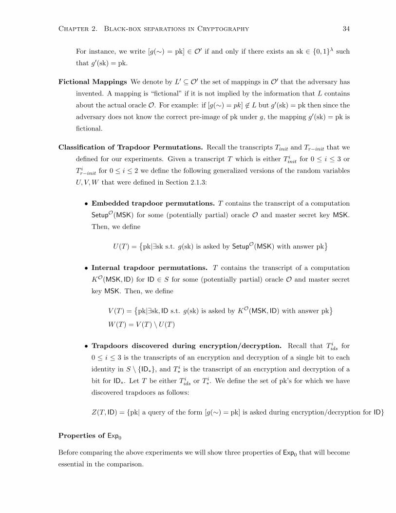
Chapter 2. Black-box separations in Cryptography 34
For instance, we write [g(∼) = pk] ∈ O′ if and only if there exists an sk ∈ 0, 1λ such
that g′(sk) = pk.
Fictional Mappings We denote by L′ ⊆ O′ the set of mappings in O′ that the adversary has
invented. A mapping is “fictional” if it is not implied by the information that L contains
about the actual oracle O. For example: if [g(∼) = pk] 6∈ L but g′(sk) = pk then since the
adversary does not know the correct pre-image of pk under g, the mapping g′(sk) = pk is
fictional.
Classification of Trapdoor Permutations. Recall the transcripts Tinit and Tr−init that we
defined for our experiments. Given a transcript T which is either T iinit for 0 ≤ i ≤ 3 or
T ir−init for 0 ≤ i ≤ 2 we define the following generalized versions of the random variables
U, V,W that were defined in Section 2.1.3:
• Embedded trapdoor permutations. T contains the transcript of a computation
SetupO(MSK) for some (potentially partial) oracle O and master secret key MSK.
Then, we define
U(T ) =
pk|∃sk s.t. g(sk) is asked by SetupO(MSK) with answer pk
• Internal trapdoor permutations. T contains the transcript of a computation
KO(MSK, ID) for ID ∈ S for some (potentially partial) oracle O and master secret
key MSK. Then, we define
V (T ) =
pk|∃sk, ID s.t. g(sk) is asked by KO(MSK, ID) with answer pk
W (T ) = V (T ) \ U(T )
• Trapdoors discovered during encryption/decryption. Recall that T iids for
0 ≤ i ≤ 3 is the transcripts of an encryption and decryption of a single bit to each
identity in S \ ID∗, and T i∗ is the transcript of an encryption and decryption of a
bit for ID∗. Let T be either T iids or T i∗. We define the set of pk’s for which we have
discovered trapdoors as follows:
Z(T, ID) = pk| a query of the form [g(∼) = pk] is asked during encryption/decryption for ID
Properties of Exp0
Before comparing the above experiments we will show three properties of Exp0 that will become
essential in the comparison.
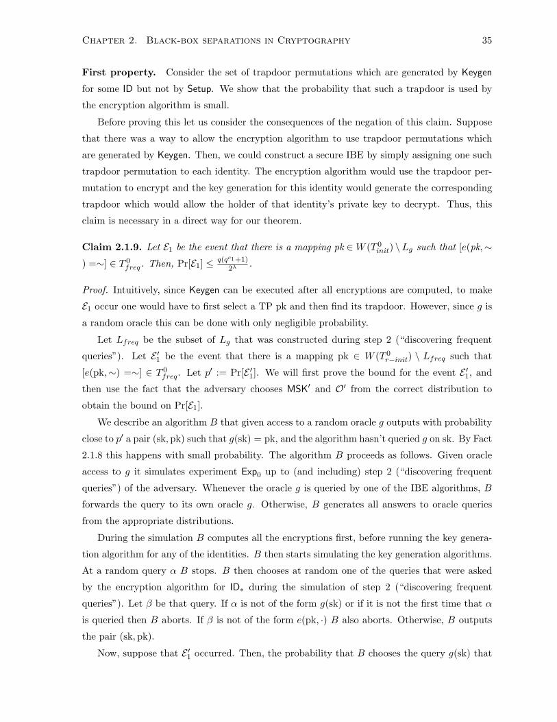
Chapter 2. Black-box separations in Cryptography 35
First property. Consider the set of trapdoor permutations which are generated by Keygen
for some ID but not by Setup. We show that the probability that such a trapdoor is used by
the encryption algorithm is small.
Before proving this let us consider the consequences of the negation of this claim. Suppose
that there was a way to allow the encryption algorithm to use trapdoor permutations which
are generated by Keygen. Then, we could construct a secure IBE by simply assigning one such
trapdoor permutation to each identity. The encryption algorithm would use the trapdoor per-
mutation to encrypt and the key generation for this identity would generate the corresponding
trapdoor which would allow the holder of that identity’s private key to decrypt. Thus, this
claim is necessary in a direct way for our theorem.
Claim 2.1.9. Let E1 be the event that there is a mapping pk ∈W (T 0init) \Lg such that [e(pk,∼
) =∼] ∈ T 0freq. Then, Pr[E1] ≤ q(qc1+1)
2λ.
Proof. Intuitively, since Keygen can be executed after all encryptions are computed, to make
E1 occur one would have to first select a TP pk and then find its trapdoor. However, since g is
a random oracle this can be done with only negligible probability.
Let Lfreq be the subset of Lg that was constructed during step 2 (“discovering frequent
queries”). Let E ′1 be the event that there is a mapping pk ∈ W (T 0r−init) \ Lfreq such that
[e(pk,∼) =∼] ∈ T 0freq. Let p′ := Pr[E ′1]. We will first prove the bound for the event E ′1, and
then use the fact that the adversary chooses MSK′ and O′ from the correct distribution to
obtain the bound on Pr[E1].
We describe an algorithm B that given access to a random oracle g outputs with probability
close to p′ a pair (sk,pk) such that g(sk) = pk, and the algorithm hasn’t queried g on sk. By Fact
2.1.8 this happens with small probability. The algorithm B proceeds as follows. Given oracle
access to g it simulates experiment Exp0 up to (and including) step 2 (“discovering frequent
queries”) of the adversary. Whenever the oracle g is queried by one of the IBE algorithms, B
forwards the query to its own oracle g. Otherwise, B generates all answers to oracle queries
from the appropriate distributions.
During the simulation B computes all the encryptions first, before running the key genera-
tion algorithm for any of the identities. B then starts simulating the key generation algorithms.
At a random query α B stops. B then chooses at random one of the queries that were asked
by the encryption algorithm for ID∗ during the simulation of step 2 (“discovering frequent
queries”). Let β be that query. If α is not of the form g(sk) or if it is not the first time that α
is queried then B aborts. If β is not of the form e(pk, ·) B also aborts. Otherwise, B outputs
the pair (sk,pk).
Now, suppose that E ′1 occurred. Then, the probability that B chooses the query g(sk) that
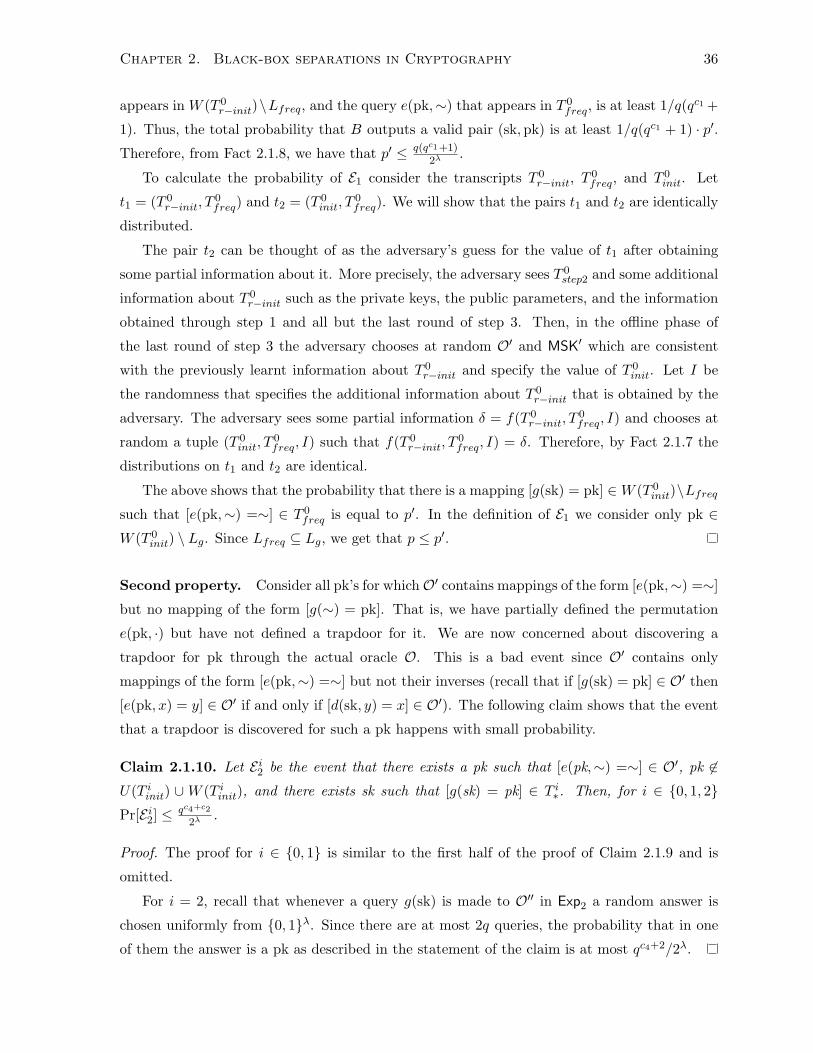
Chapter 2. Black-box separations in Cryptography 36
appears in W (T 0r−init)\Lfreq, and the query e(pk,∼) that appears in T 0
freq, is at least 1/q(qc1 +
1). Thus, the total probability that B outputs a valid pair (sk,pk) is at least 1/q(qc1 + 1) · p′.Therefore, from Fact 2.1.8, we have that p′ ≤ q(qc1+1)
2λ.
To calculate the probability of E1 consider the transcripts T 0r−init, T
0freq, and T 0
init. Let
t1 = (T 0r−init, T
0freq) and t2 = (T 0
init, T0freq). We will show that the pairs t1 and t2 are identically
distributed.
The pair t2 can be thought of as the adversary’s guess for the value of t1 after obtaining
some partial information about it. More precisely, the adversary sees T 0step2 and some additional
information about T 0r−init such as the private keys, the public parameters, and the information
obtained through step 1 and all but the last round of step 3. Then, in the offline phase of
the last round of step 3 the adversary chooses at random O′ and MSK′ which are consistent
with the previously learnt information about T 0r−init and specify the value of T 0
init. Let I be
the randomness that specifies the additional information about T 0r−init that is obtained by the
adversary. The adversary sees some partial information δ = f(T 0r−init, T
0freq, I) and chooses at
random a tuple (T 0init, T
0freq, I) such that f(T 0
r−init, T0freq, I) = δ. Therefore, by Fact 2.1.7 the
distributions on t1 and t2 are identical.
The above shows that the probability that there is a mapping [g(sk) = pk] ∈W (T 0init)\Lfreq
such that [e(pk,∼) =∼] ∈ T 0freq is equal to p′. In the definition of E1 we consider only pk ∈
W (T 0init) \ Lg. Since Lfreq ⊆ Lg, we get that p ≤ p′.
Second property. Consider all pk’s for whichO′ contains mappings of the form [e(pk,∼) =∼]
but no mapping of the form [g(∼) = pk]. That is, we have partially defined the permutation
e(pk, ·) but have not defined a trapdoor for it. We are now concerned about discovering a
trapdoor for pk through the actual oracle O. This is a bad event since O′ contains only
mappings of the form [e(pk,∼) =∼] but not their inverses (recall that if [g(sk) = pk] ∈ O′ then
[e(pk, x) = y] ∈ O′ if and only if [d(sk, y) = x] ∈ O′). The following claim shows that the event
that a trapdoor is discovered for such a pk happens with small probability.
Claim 2.1.10. Let E i2 be the event that there exists a pk such that [e(pk,∼) =∼] ∈ O′, pk 6∈U(T iinit) ∪W (T iinit), and there exists sk such that [g(sk) = pk] ∈ T i∗. Then, for i ∈ 0, 1, 2Pr[E i2] ≤ qc4+c2
2λ.
Proof. The proof for i ∈ 0, 1 is similar to the first half of the proof of Claim 2.1.9 and is
omitted.
For i = 2, recall that whenever a query g(sk) is made to O′′ in Exp2 a random answer is
chosen uniformly from 0, 1λ. Since there are at most 2q queries, the probability that in one
of them the answer is a pk as described in the statement of the claim is at most qc4+2/2λ.
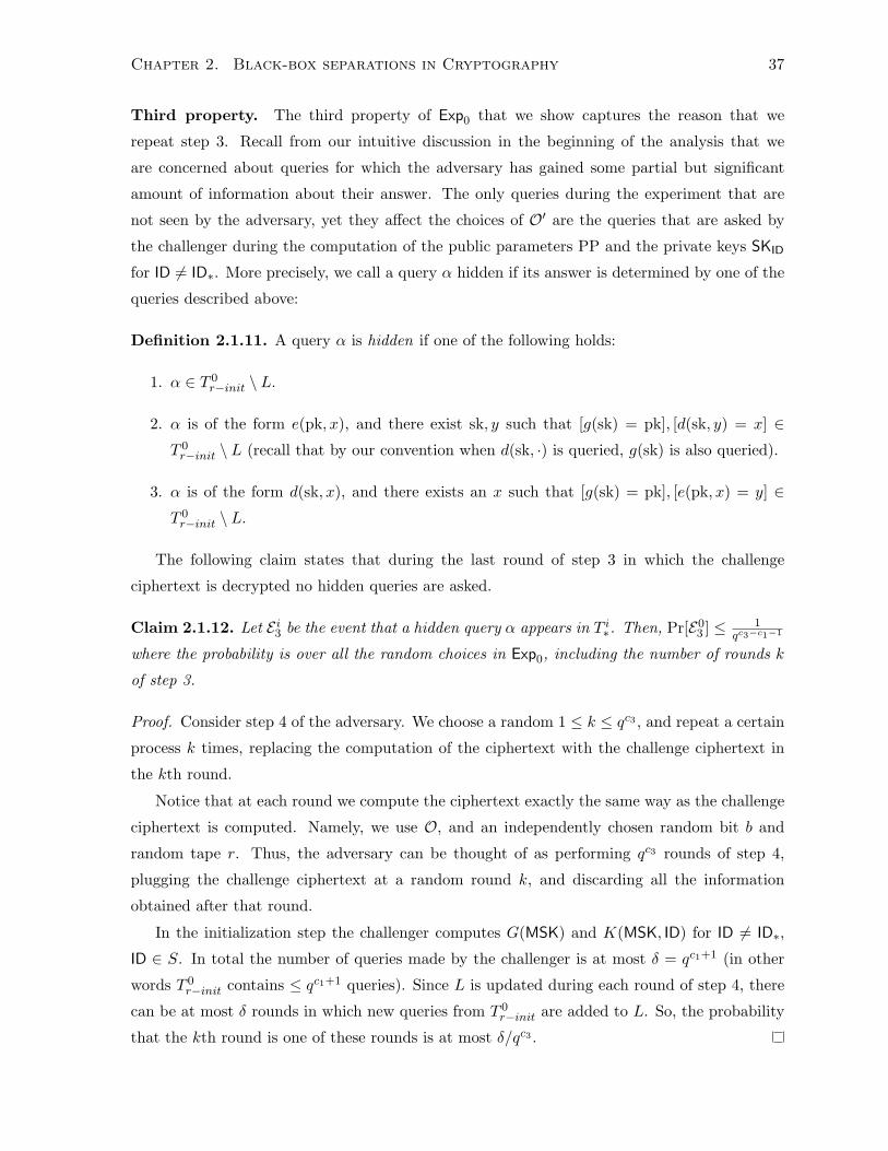
Chapter 2. Black-box separations in Cryptography 37
Third property. The third property of Exp0 that we show captures the reason that we
repeat step 3. Recall from our intuitive discussion in the beginning of the analysis that we
are concerned about queries for which the adversary has gained some partial but significant
amount of information about their answer. The only queries during the experiment that are
not seen by the adversary, yet they affect the choices of O′ are the queries that are asked by
the challenger during the computation of the public parameters PP and the private keys SKID
for ID 6= ID∗. More precisely, we call a query α hidden if its answer is determined by one of the
queries described above:
Definition 2.1.11. A query α is hidden if one of the following holds:
1. α ∈ T 0r−init \ L.
2. α is of the form e(pk, x), and there exist sk, y such that [g(sk) = pk], [d(sk, y) = x] ∈T 0r−init \ L (recall that by our convention when d(sk, ·) is queried, g(sk) is also queried).
3. α is of the form d(sk, x), and there exists an x such that [g(sk) = pk], [e(pk, x) = y] ∈T 0r−init \ L.
The following claim states that during the last round of step 3 in which the challenge
ciphertext is decrypted no hidden queries are asked.
Claim 2.1.12. Let E i3 be the event that a hidden query α appears in T i∗. Then, Pr[E03 ] ≤ 1
qc3−c1−1
where the probability is over all the random choices in Exp0, including the number of rounds k
of step 3.
Proof. Consider step 4 of the adversary. We choose a random 1 ≤ k ≤ qc3 , and repeat a certain
process k times, replacing the computation of the ciphertext with the challenge ciphertext in
the kth round.
Notice that at each round we compute the ciphertext exactly the same way as the challenge
ciphertext is computed. Namely, we use O, and an independently chosen random bit b and
random tape r. Thus, the adversary can be thought of as performing qc3 rounds of step 4,
plugging the challenge ciphertext at a random round k, and discarding all the information
obtained after that round.
In the initialization step the challenger computes G(MSK) and K(MSK, ID) for ID 6= ID∗,
ID ∈ S. In total the number of queries made by the challenger is at most δ = qc1+1 (in other
words T 0r−init contains ≤ qc1+1 queries). Since L is updated during each round of step 4, there
can be at most δ rounds in which new queries from T 0r−init are added to L. So, the probability
that the kth round is one of these rounds is at most δ/qc3 .
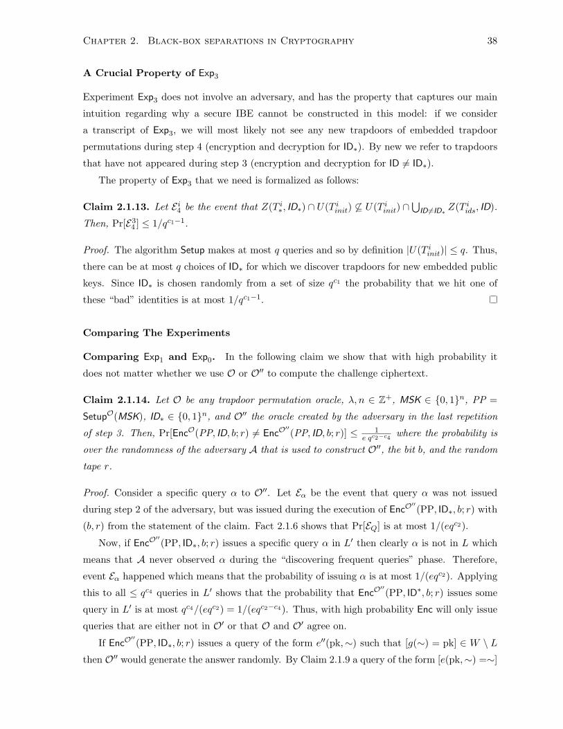
Chapter 2. Black-box separations in Cryptography 38
A Crucial Property of Exp3
Experiment Exp3 does not involve an adversary, and has the property that captures our main
intuition regarding why a secure IBE cannot be constructed in this model: if we consider
a transcript of Exp3, we will most likely not see any new trapdoors of embedded trapdoor
permutations during step 4 (encryption and decryption for ID∗). By new we refer to trapdoors
that have not appeared during step 3 (encryption and decryption for ID 6= ID∗).
The property of Exp3 that we need is formalized as follows:
Claim 2.1.13. Let E i4 be the event that Z(T i∗, ID∗) ∩ U(T iinit) 6⊆ U(T iinit) ∩⋃
ID6=ID∗Z(T iids, ID).
Then, Pr[E34 ] ≤ 1/qc1−1.
Proof. The algorithm Setup makes at most q queries and so by definition |U(T iinit)| ≤ q. Thus,
there can be at most q choices of ID∗ for which we discover trapdoors for new embedded public
keys. Since ID∗ is chosen randomly from a set of size qc1 the probability that we hit one of
these “bad” identities is at most 1/qc1−1.
Comparing The Experiments
Comparing Exp1 and Exp0. In the following claim we show that with high probability it
does not matter whether we use O or O′′ to compute the challenge ciphertext.
Claim 2.1.14. Let O be any trapdoor permutation oracle, λ, n ∈ Z+, MSK ∈ 0, 1n, PP =
SetupO(MSK), ID∗ ∈ 0, 1n, and O′′ the oracle created by the adversary in the last repetition
of step 3. Then, Pr[EncO(PP, ID, b; r) 6= EncO′′(PP, ID, b; r)] ≤ 1
e qc2−c4where the probability is
over the randomness of the adversary A that is used to construct O′′, the bit b, and the random
tape r.
Proof. Consider a specific query α to O′′. Let Eα be the event that query α was not issued
during step 2 of the adversary, but was issued during the execution of EncO′′(PP, ID∗, b; r) with
(b, r) from the statement of the claim. Fact 2.1.6 shows that Pr[EQ] is at most 1/(eqc2).
Now, if EncO′′(PP, ID∗, b; r) issues a specific query α in L′ then clearly α is not in L which
means that A never observed α during the “discovering frequent queries” phase. Therefore,
event Eα happened which means that the probability of issuing α is at most 1/(eqc2). Applying
this to all ≤ qc4 queries in L′ shows that the probability that EncO′′(PP, ID∗, b; r) issues some
query in L′ is at most qc4/(eqc2) = 1/(eqc2−c4). Thus, with high probability Enc will only issue
queries that are either not in O′ or that O and O′ agree on.
If EncO′′(PP, ID∗, b; r) issues a query of the form e′′(pk,∼) such that [g(∼) = pk] ∈ W \ L
then O′′ would generate the answer randomly. By Claim 2.1.9 a query of the form [e(pk,∼) =∼]
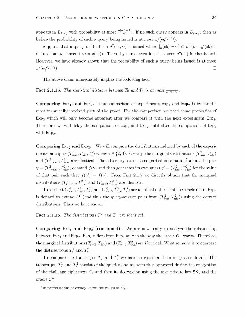
Chapter 2. Black-box separations in Cryptography 39
appears in Lfreq with probability at most q(qc1+1)2λ
. If no such query appears in Lfreq, then as
before the probability of such a query being issued is at most 1/(eqc2−c4).
Suppose that a query of the form d′′(sk,∼) is issued where [g(sk) =∼] ∈ L′ (i.e. g′(sk) is
defined but we haven’t seen g(sk)). Then, by our convention the query g′′(sk) is also issued.
However, we have already shown that the probability of such a query being issued is at most
1/(eqc2−c4).
The above claim immediately implies the following fact:
Fact 2.1.15. The statistical distance between T0 and T1 is at most 1eqc2−c4
.
Comparing Exp1 and Exp2. The comparison of experiments Exp1 and Exp2 is by far the
most technically involved part of the proof. For the comparison we need some properties of
Exp2 which will only become apparent after we compare it with the next experiment Exp3.
Therefore, we will delay the comparison of Exp1 and Exp2 until after the comparison of Exp1
with Exp2.
Comparing Exp2 and Exp3. We will compare the distributions induced by each of the experi-
ments on triples (T iinit, Tiids, T
i∗) where i ∈ 2, 3. Clearly, the marginal distributions (T 3
init, T3ids)
and (T 2r−init, T
2ids) are identical. The adversary learns some partial information5 about the pair
γ = (T 2r−init, T
2ids), denoted f(γ) and then generates its own guess γ′ = (T 2
init, T2ids) for the value
of that pair such that f(γ′) = f(γ). From Fact 2.1.7 we directly obtain that the marginal
distributions (T 2r−init, T
2ids) and (T 2
init, T2ids) are identical.
To see that (T 2init, T
2ids, T
2∗ ) and (T 3
init, T3ids, T
3∗ ) are identical notice that the oracle O′′ in Exp2
is defined to extend O′ (and thus the query-answer pairs from (T 2init, T
2ids)) using the correct
distributions. Thus we have shown
Fact 2.1.16. The distributions T 2 and T 3 are identical.
Comparing Exp1 and Exp2 (continued). We are now ready to analyze the relationship
between Exp1 and Exp2. Exp2 differs from Exp1 only in the way the oracle O′′ works. Therefore,
the marginal distributions (T 1init, T
1ids) and (T 2
init, T2ids) are identical. What remains is to compare
the distributions T 1∗ and T 2
∗ .
To compare the transcripts T 1∗ and T 2
∗ we have to consider them in greater detail. The
transcripts T 1∗ and T 2
∗ consist of the queries and answers that appeared during the encryption
of the challenge ciphertext C∗ and then its decryption using the fake private key SK′∗ and the
oracle O′′.5In particular the adversary knows the values of T 2
ids
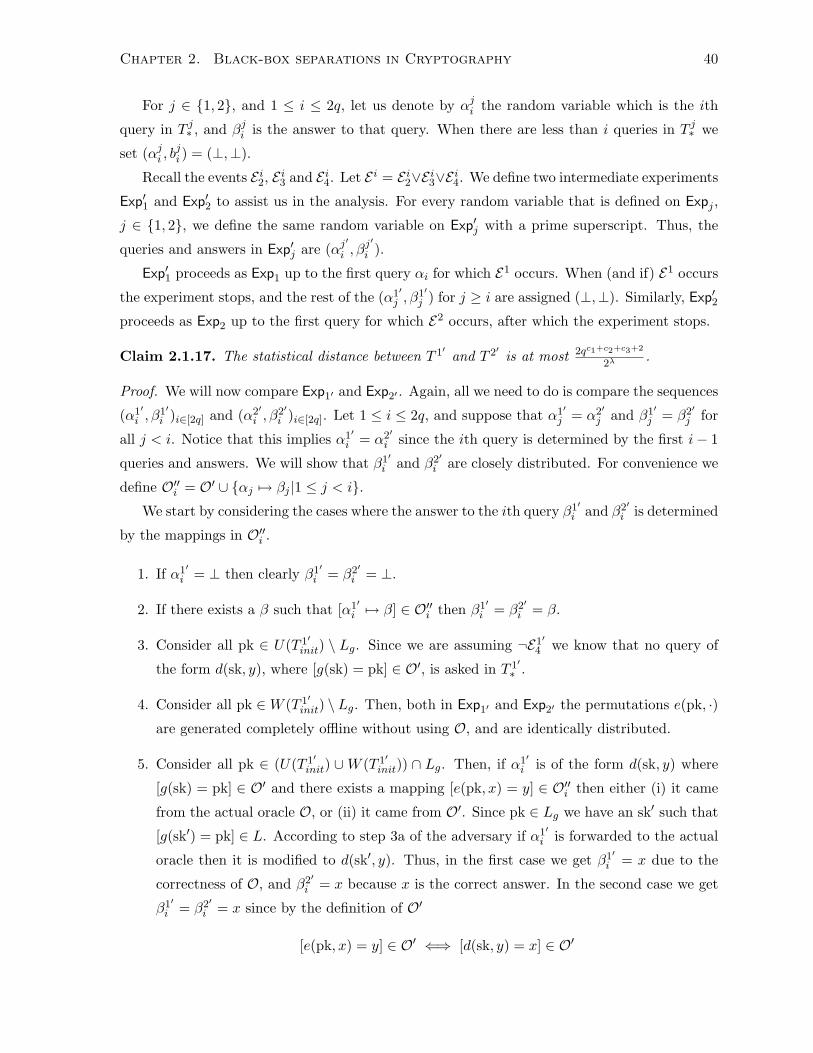
Chapter 2. Black-box separations in Cryptography 40
For j ∈ 1, 2, and 1 ≤ i ≤ 2q, let us denote by αji the random variable which is the ith
query in T j∗ , and βji is the answer to that query. When there are less than i queries in T j∗ we
set (αji , bji ) = (⊥,⊥).
Recall the events E i2, E i3 and E i4. Let E i = E i2∨E i3∨E i4. We define two intermediate experiments
Exp′1 and Exp′2 to assist us in the analysis. For every random variable that is defined on Expj ,
j ∈ 1, 2, we define the same random variable on Exp′j with a prime superscript. Thus, the
queries and answers in Exp′j are (αj′
i , βj′
i ).
Exp′1 proceeds as Exp1 up to the first query αi for which E1 occurs. When (and if) E1 occurs
the experiment stops, and the rest of the (α1′j , β
1′j ) for j ≥ i are assigned (⊥,⊥). Similarly, Exp′2
proceeds as Exp2 up to the first query for which E2 occurs, after which the experiment stops.
Claim 2.1.17. The statistical distance between T 1′ and T 2′ is at most 2qc1+c2+c3+2
2λ.
Proof. We will now compare Exp1′ and Exp2′ . Again, all we need to do is compare the sequences
(α1′i , β
1′i )i∈[2q] and (α2′
i , β2′i )i∈[2q]. Let 1 ≤ i ≤ 2q, and suppose that α1′
j = α2′j and β1′
j = β2′j for
all j < i. Notice that this implies α1′i = α2′
i since the ith query is determined by the first i− 1
queries and answers. We will show that β1′i and β2′
i are closely distributed. For convenience we
define O′′i = O′ ∪ αj 7→ βj |1 ≤ j < i.We start by considering the cases where the answer to the ith query β1′
i and β2′i is determined
by the mappings in O′′i .
1. If α1′i = ⊥ then clearly β1′
i = β2′i = ⊥.
2. If there exists a β such that [α1′i 7→ β] ∈ O′′i then β1′
i = β2′i = β.
3. Consider all pk ∈ U(T 1′init) \ Lg. Since we are assuming ¬E1′
4 we know that no query of
the form d(sk, y), where [g(sk) = pk] ∈ O′, is asked in T 1′∗ .
4. Consider all pk ∈W (T 1′init) \ Lg. Then, both in Exp1′ and Exp2′ the permutations e(pk, ·)
are generated completely offline without using O, and are identically distributed.
5. Consider all pk ∈ (U(T 1′init) ∪W (T 1′
init)) ∩ Lg. Then, if α1′i is of the form d(sk, y) where
[g(sk) = pk] ∈ O′ and there exists a mapping [e(pk, x) = y] ∈ O′′i then either (i) it came
from the actual oracle O, or (ii) it came from O′. Since pk ∈ Lg we have an sk′ such that
[g(sk′) = pk] ∈ L. According to step 3a of the adversary if α1′i is forwarded to the actual
oracle then it is modified to d(sk′, y). Thus, in the first case we get β1′i = x due to the
correctness of O, and β2′i = x because x is the correct answer. In the second case we get
β1′i = β2′
i = x since by the definition of O′
[e(pk, x) = y] ∈ O′ ⇐⇒ [d(sk, y) = x] ∈ O′
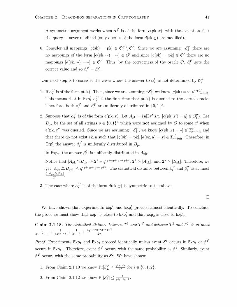
Chapter 2. Black-box separations in Cryptography 41
A symmetric argument works when α1′i is of the form e(pk, x), with the exception that
the query is never modified (only queries of the form d(sk, y) are modified).
6. Consider all mappings [g(sk) = pk] ∈ O′′i \ O′. Since we are assuming ¬E1′2 there are
no mappings of the form [e(pk,∼) =∼] ∈ O′ and since [g(sk) = pk] 6∈ O′ there are no
mappings [d(sk,∼) =∼] ∈ O′. Thus, by the correctness of the oracle O, β1′i gets the
correct value and so β1′i = β2′
i .
Our next step is to consider the cases where the answer to α1′i is not determined by O′′i .
1. If α1′i is of the form g(sk). Then, since we are assuming ¬E1′
3 we know [g(sk) =∼] 6∈ T 1′r−init.
This means that in Exp′1 α1′i is the first time that g(sk) is queried to the actual oracle.
Therefore, both β1′i and β2′
i are uniformly distributed in 0, 1λ.
2. Suppose that α1′i is of the form e(pk, x). Let Apk = y|∃x′ s.t. [e(pk, x′) = y] ∈ O′′i . Let
Bpk be the set of all strings y ∈ 0, 1λ which were not assigned by O to some x′ when
e(pk, x′) was queried. Since we are assuming ¬E1′3 , we know [e(pk, x) =∼] 6∈ T 1′
r−init and
that there do not exist sk, y such that [g(sk) = pk], [d(sk, y) = x] ∈ T 1′r−init. Therefore, in
Exp′1 the answer β1′i is uniformly distributed in Bpk.
In Exp′2, the answer β2′i is uniformly distributed in Apk.
Notice that |Apk ∩Bpk| ≥ 2λ − qc1+c2+c3+c4+2, 2λ ≥ |Apk|, and 2λ ≥ |Bpk|. Therefore, we
get |Apk4Bpk|| ≤ qc1+c2+c3+c4+2. The statistical distance between β1′i and β2′
i is at most2|Apk4Bpk|
2λ.
3. The case where α1′i is of the form d(sk, y) is symmetric to the above.
We have shown that experiments Exp′1 and Exp′2 proceed almost identically. To conclude
the proof we must show that Exp1 is close to Exp′1 and that Exp2 is close to Exp′2.
Claim 2.1.18. The statistical distance between T 1 and T 1′ and between T 2 and T 2′ is at most1
qc3−c1−1 + 1eqc2−c4
+ 1qc1−1 + 4qc1+c2+c3+c4+2
2λ
Proof. Experiments Exp1 and Exp′1 proceed identically unless event E1 occurs in Exp1 or E1′
occurs in Exp1′ . Therefore, event E1′ occurs with the same probability as E1. Similarly, event
E2′ occurs with the same probability as E2. We have shown:
1. From Claim 2.1.10 we know Pr[E i2] ≤ qc4+c2
2λfor i ∈ 0, 1, 2.
2. From Claim 2.1.12 we know Pr[E03 ] ≤ 1
qc3−c1−1 .
Chapter 2. Black-box separations in Cryptography 42
3. From Claim 2.1.13 we know Pr[E34 ] ≤ 1
qc1−1 .
By applying Fact 2.1.15 we get Pr[E1′3 ] ≤ Pr[E0
3 ] + 1eqc2−c4
. By applying Fact 2.1.16 we get
Pr[E2′4 ] = Pr[E3
4 ]. Now, by applying Claim 2.1.17 we get
1. Pr[E2′3 ] ≤ 1
qc3−c1−1 + 1eqc2−c4
+ 2qc1+c2+c3+c4+2
2λ.
2. Pr[E1′4 ] ≤ 1
qc1−1 + 2qc1+c2+c3+c4+2
2λ.
Thus we have
Pr[E1′ ] ≤ Pr[E1′2 ] + Pr[E1′
3 ] + Pr[E1′4 ]
≤ qc4+c2
2λ+
1qc3−c1−1
+1
eqc2−c4+
1qc1−1
+2qc1+c2+c3+c4+2
2λ
≤ 1qc3−c1−1
+1
eqc2−c4+
1qc1−1
+4qc1+c2+c3+c4+2
2λPr[E2′ ] ≤ Pr[E2′
2 ] + Pr[E2′3 ] + Pr[E2′
4 ]
≤ qc4+c2
2λ+
1qc3−c1−1
+1
eqc2−c4+
2qc1+c2+c3+c4+2
2λ+
1qc1−1
≤ 1qc3−c1−1
+1
eqc2−c4+
4qc1+c2+c3+c4+2
2λ+
1qc1−1
Summing Up. We have described a series of closely related experiment where the first exper-
iment is the security game of the IBE, and the last experiment does not involve an adversary. It
is easy to see that in Exp3 the ciphertext C∗ is decrypted with probability ε, which is guaranteed
by the correctness property of the IBE. Combining this with Claim 2.1.18, Fact 2.1.16, Fact
2.1.15, and Claim 2.1.17 we obtain our theorem:
Claim 2.1.19. The probability of the adversary correctly decrypting the challenge ciphertext is
at least ε−(
2qc3−c1−1 + 3
eqc2−c4+ 2
qc1−1 + 10qc1+c2+c3+c4+2
2λ
)
2.2 Towards a black-box separation of IBE from DDH
We ask whether Identity Based Encryption (IBE) can be based in a black-box way on the
average-case hardness of Decisional Diffie-Hellman (DDH). Conceptually, this would answer
in some sense why many known constructions of IBEs rely on bilinear pairings, which are
generalizations of DDH, and not the DDH itself. The DDH assumption is very well-studied,
and it finds a surprising number of applications in cryptographic constructions; see e.g. [Bon98]
for a not-so-recent survey.
On the technical side, to the best of our knowledge there are no prior black-box separations
of any cryptographic primitive from DDH. We present the setting where we aim to do the
Chapter 2. Black-box separations in Cryptography 43
black-box separation, and we also present some preliminary results towards this separation. In
particular, we show a reduction from an arbitrary IBE system to a restricted IBE. Technically
speaking, separating IBE from DDH is significantly more complicated than the separation
from TDPs. The reduction we present deals with the main technical difference between this
impossibility result and the one described in Section 2.1. Although it is not possible to compare
with the details of work in progress, after the description of the model we give a rough idea of
what this reduction achieves. There are also several other details and technical differences that
need to be taken care of for the full argument to work. We leave those for a future paper.
One interesting feature of this black-box separation is the setting itself. To put things in
the proper context let us first recall the DDH assumption.
Assumption 2 (Decisional Diffie Hellman (DDH)). There exists an infinite family of encodings
of cyclic groups Gn (say in additive notation), gn, pn, where gn is a generator of Gn, of
prime order pn. Gn is encoded as a subset of 0, 1nO(1), such that (1) there exists a deterministic
polynomial time algorithm that given pn, gn and x, y ∈ Gn it computes the value of x+ y, and
(2) for every probabilistic polynomial time adversary A and for sufficiently large n:
| Pra,b∈R0,1,...,pn−1
[A(1n, pn, g, a·g, b·g, (ab)·g) = 1]− Pra,b,c∈R0,1,...,pn−1
[A(1n, pn, g, a·g, b·g, c·g) = 1]| ≤ 1nk
Our black-box setting uses an oracle which realizes a primitive where DDH holds, and
furthermore DDH is naturally related to the primitive in the oracle. At the same time we aim
to show that the security of every IBE can be broken in this setting.
The intuition behind the average-case hardness of DDH is that for the family of groups
of choice the group elements look random. Shoup [Sho97] formalized a model of computation
where the group elements are random, by an appropriate random embedding of Zn := Z/nZ,
n ∈ Z, into a finite set of strings.
Definition 2.2.1 (Generic Groups Model). Let n ∈ Z+ be a parameter, and 2n−1 < p < 2n be
a prime. Let σ : Zp → S, |S| ≥ p, be an injective function inducing a subgroup on the image
σ(Zp). We call σ an encoding function of Zp. A generic algorithm A for Zp on a finite S is
a probabilistic algorithm with access to a random σ and inputs consisting of a string and of
group elements of the form 〈w, σ(a1), . . . , σ(ak)〉, where w ∈ 0, 1∗. A computes as follows: at
each step the algorithm specifies a linear combination on the σ(ai)’s. This linear combination
is determined as a function of w and the group elements σ(x) the algorithm A has seen so far
(either in the input or in the history of answers to previous queries). The linear combination is
a query to the oracle realizing the group operation, which returns the resulting group element
Chapter 2. Black-box separations in Cryptography 44
σ(y). At the end of the computation A outputs6 〈w′, σ(b1), . . . , σ(bm)〉, w′ ∈ 0, 1∗.
Note that in this definition A is strongly non-uniform. As usual, the complexity measure
is the number of oracle queries. The intuition in this definition is that Zp is encoded in a
way that no information about other group elements can be extracted by the presented group
element (recall that the encoding σ is chosen at random). Intuitively, the only relation that the
algorithm may test between group elements is equality. This definition formalizes the intuition
that groups for which the Discrete Logarithm (DL) is hard are those satisfying this intuitive
property. In fact, Shoup [Sho97] shows that in this model7 DL is hard. Similarly it can be
shown that Assumption 2 holds true in the Generic Groups model. In particular, Public Key
Encryption (PKE) exists in this setting.; e.g. the Cramer-Shoup cryptosystem [CS98] is CCA
secure given DDH. This is an important distinction from the black-box separation in [IR88].
Let us recall the El-Gamal encryption system, which is based on the hardness of DDH, it is
simpler than the Cramer-Shoup, but it is only semantically secure.
Motivating discussion: El-Gamal. We describe a well-known Public-Key Encryption sys-
tem (conceptually based on the Diffie-Hellman key-exchange). This is known as the El-Gamal
encryption system [ElG85]. It is semantically secure assuming that DDH is hard, and thus good
enough (see Section 2.1.1 for the security notion we use for IBE) for this motivating discussion.
Recall, that a PKE system is a special case of an IBE. It consists of three algorithms: key-
generation, encryption, and decryption. Keygen outputs a public PUB and a private key SK.
As usual, PUB is used for encryption, and SK is used for decryption. Here is the description of
the El-Gamal PKE system.
We describe this PKE system in the Generic Groups Model. Suppose that the three al-
gorithms have access to the same oracle O for the operations of the group G. For notational
simplicity we omit denoting the oracle when no confusion arises; e.g. we write Keygen instead
of KeygenO. We encrypt/decrypt group elements (i.e. the message is just a group element). In
the following description, the strings corresponding to randomness are identified by integers.
Keygen(g1, r): Use the randomness r and the generator g1 of G to sample an element h := r ·g1.
Output: PUB = (h, g1) and SK = r.
Enc((h, g1)︸ ︷︷ ︸PUB
, g, r′): The group element g is the message we wish to encrypt. Output the cipher
c = (c1, c2), where c1 = r′ · g1 and c2 = r′ · h+ g.
6This notation does not imply that A knows the bi’s (in fact, in general this is impossible). An element σ(bi)is presented to A as an answer to a query regarding a linear combination of the σ(ai)’s.
7The model considered by Shoup is equivalent, but notationally less convenient for our purposes.
Chapter 2. Black-box separations in Cryptography 45
Dec( r︸︷︷︸SK
, (c1, c2)): Output c2 − (r · c1).
Correctness is immediate by definition. Keygen outputs public key (r · g1, g1); then for a
message g, Enc outputs c = (r′ · g1, r′ · (r · g1) + g); and on input c, Dec outputs r′ · (r · g1) +
g − r · (r′ · g1) = g.
It is also semantically secure in the Generic Groups Model. Its security follows by the
hardness of DDH, and DDH is hard in the Generic Groups Model.
Imagine that we modify the above scheme as follows. Partition r into nk many contiguous
blocks, each of which is of polynomial size, and generate the pair:
MPUB = (r1 · g1, r1 · g2, . . . , rnk · gnk), MSK = (r1, r2, . . . , rnk)
Associate each “subpair” (rig1, ri) with a particular identity. Then, it is obvious how to extend
the El-Gamal cryptosystem to an IBE-like one, where we rename Keygen to Setup, and we
construct a new Keygen which issues the “subpairs” for the relevant identities.
By the properties of El-Gamal, it is obvious that this IBE-like system works only for at
most nk identities, and it works securely. However, as the number of identities becomes enough
bigger than nk then no matter how you modify this encryption system, it must be the case
that there will be “relations” among the private (secret) keys associated with identities. In
our separation argument (which is work in progress) we identify these “relations” as linear
relations over appropriate vector spaces, and we construct an adversary that finds them in time
polynomial in the maximum number of queries an IBE algorithm makes.
2.2.1 Definitions and notational conventions (differences with Section 2.1).
All algorithms in an IBE are generic with access to the same oracle O. We describe the oracle
and relevant notation below. The four algorithms are (SetupO,KeygenO,EncO,DecO); we omit
O when it is clear from the context. The input to each algorithm is a string and a tuple of
group elements: 〈w, σ(a1), . . . , σ(am)〉, and the same holds for the output. As in Section 2.1.1,
here too we consider the possibility of WSS-IBEs, with noticeable correctness; where noticeable
probability means that there is a constant c > 0 such that for sufficiently large n, the probability
is ≥ 1nc .
In Section 2.1 (and other related works) many parameters are used, e.g. λ is the security
parameter, n corresponds to input length etc. In this section we reduce notational clutter and
we focus on the useful and typical case8.
Parameters. Instead of λ, n, q, ε we have:
8Recall that this reduction would be part of a general impossibility result, where it makes sense to considerdifferent cases for the proof as a whole.
Chapter 2. Black-box separations in Cryptography 46
• n: the security parameter. According to Definition 2.2.1 the group is of order p ≈ 2n.
• ε: the IBE is correct with probability ≥ ε > 12 over the randomness in the security
experiment.
• k: every algorithm in the IBE makes ≤ nk queries. Let m := nk.
The oracle O. We introduce the notation regarding oracle access; i.e. queries and how to
answer them. Let n, p be as in Definition 2.2.1; i.e. p ≈ 2n. Let σ : Zp → 0, 1n a random
embedding. We denote by G = σ(Zp) the induced group in additive notation. We write 0 to
denote σ(0), the n-bit string which is the identity element of G. Recall that for any finite set S
the set of formal sums Zp[S] is an |S|-dimensional vector space in the usual sense. In particular,
we will treat Zp[G] as a vector space. Occasionally, we write linear combinations of elements
of G to refer to formal sums in Zp[G]. For Zp[G] the group structure of G becomes relevant
through the valuation map. We denote by O the valuation map O : Zp[G] → G defined as
follows. For α ∈ Zp and u ∈ G, αg := g +G g +G . . .+G g︸ ︷︷ ︸α times
, where +G is the group operation.
The formal sum α1g1 +α2g2 + . . .+αkgk valuates through O to a group element where instead
of + we consider +G. Henceforth, we use + instead of +G when no confusion arises.
In an IBE system the four algorithms have access to the same valuation O, but each algo-
rithm is restricted to different oracle-access in the following sense. If the input to an algorithm
A is 〈w, g1, g2, . . . , gm〉, w ∈ 0, 1∗ and gi ∈ G then every query of A is of the form∑m
i=1 αigi;
i.e. the access to oracle O is restricted to valuations of formal sums of S = g1, . . . , gm. Note
that Zp[S] is a subspace of Zp[G]. We also make the convention that the first group element in
the input and output (if the output contains any group elements) of a generic algorithm is a
generator of the group (i.e. 6= 0, since G ≈ Zp).
We use the following terms interchangeably. A query q of an algorithm is a formal sum of
its input elements. An answer to a query q is a valuation.
2.2.2 The Theorem
Let IBEO = (SetupO,KeygenO,EncO,DecO) be an Identity Based Encryption system where the
algorithms are generic with oracle access to O. When the oracle is clear from the context we
omit O and we write IBE . Recall that IBE comes with parameters k, ε, such that, for every n
each algorithm makes at most nk queries to O, and IBE is correct with probability ≥ ε.
Restricted Identity Based Encryption. We say that an Identity Based Encryption system
IBE ′ = (Setup′,Keygen′,Enc′,Dec′) is restricted if the Key-generation algorithm, Keygen′, out-
puts secret keys SKID that do not contain any group elements.
Chapter 2. Black-box separations in Cryptography 47
Theorem 2.2.2. Suppose that IBE = (Setup,Keygen,Enc,Dec) is a WSS-IBE, correct with
probability ≥ ε. Then, there exists ε′ > 12 and a restricted IBE, IBE ′ = (Setup′,Keygen′,Enc′,Dec′),
which is a WSS-IBE, correct with probability ≥ ε′.
Discussion on the main theorem
Why our main theorem is of any use to the black-box separation? This reduction makes the
template of the separation from DDH to look the same as for TDPs. The rest of the result is
work in progress and we aren’t going to discuss it further. However, there is an independent,
explicit, technical reason why we care about this theorem. Theorem 2.2.2 “removes” the group
elements from the output of Keygen, which are the secret keys. Now, imagine9 that we were
able to remove the group elements from the output of each of the remaining three algorithms.
Then, we claim that by [IR88] we can conclude the impossibility.
The fact that the output of the algorithms contain group elements, is where the main
technical complication happens. In particular, if no group elements were to be included in the
global public key MPUB, the secret keys SKID’s, and the ciphertexts, then the impossibility
follows by [IR88], since the group oracle acts just like a random oracle.
Elementary properties used in the reduction
The two ways10 of considering the group (as formal sums of elements, and as valuations of
formal sums) can be “mixed”, since O is in particular a group homomorphism. Here are two
trivial consequences (we mention them to emphasize their use).
Fact 2.2.3.
• Let two queries q1 :=∑k
i=1 αiui +∑l
i=1 βivi and q2 :=∑k
i=1 αiui +∑l′
i=1 γihi, where
αi, βi, γi ∈ Zp, ui, vi, hi ∈ G. Then, O(q1) = O(q2) ⇐⇒ O(∑l
i=1 βivi) = O(∑l′
i=1 γihi).
• Let qid ∈ ker(O) and q a query. Then, O(q) = O(q + qid).
Let us give a preview on some part of the reduction. At a high level IBE ′ simulates IBE .
The main issue is that in IBE ′ we wish to somehow use IBE so as to answer in Dec′ queries
involving group elements that appear in SKID. But, by definition of a restricted IBE we do not
have group elements in the secret keys. There are cases where for the same typical answer there
are many corresponding queries, expressed as distinct formal sums. The main technical part
9Note that our actual proof in progress does not work this way. It seems technically simpler to directlyconstruct an adversary against restricted IBEs.
10Loosely speaking, we reduce a general IBE to IBE ′, where IBE ′ tries to simulate answers to queries involvinggroup elements it does not know, by acting in part “syntactically” similar to a proof system, and in part it relieson the “semantics” which are the valuations of queries.
Chapter 2. Black-box separations in Cryptography 48
of our argument formalizes the following intuition: no matter which these formal sums are, as
long as they are“known” by the algorithms in IBE , then they can be obtained by syntactic
manipulations using Fact 2.2.3. Roughly speaking, our task is to find a sufficient subspace of
ker(O), and sufficiently many ways to express the same frequent answer.
2.2.3 The reduction
Fix an arbitrary IBE . Here is how we define an IBE ′ without group elements in the output of
Keygen′ with the following property. IBE ′ makes polynomially more queries than IBE , and it
preserves security and correctness within polynomial factors. Recall that m = nk.
Notation for group elements in IBE
We introduce some notation for the group elements in the inputs/outputs of the algorithms for
the IBE . We denote by m1,m2,m3,m4 ≤ m the number of group elements in the outputs of
Setup,Keygen,Enc,Dec.
• Setup: without loss of generality, the private key is the randomness for Setup, and we
denote group elements of the public key by: g1, . . . , gm1 .
• Keygen: we denote the group elements in SKID by: z1, . . . , zm2 .
• Enc: we denote the group elements of the ciphertext by: t1, . . . , tm3 .
• Dec: this algorithm does not output group elements; it decrypts the bit encrypted by Enc.
Let the (general) IBE be the tuple of algorithms IBE := (Setup,Keygen,Enc,Dec). We
define IBE ′ := (Setup′,Keygen′,Enc′,Dec′) as follows:
• Setup′: The same as Setup.
• Keygen′(PK, ID): Run (w, z1, . . . , zm)← Keygen(PK, ID).
Iteratively run Enc and Dec on ID for a randomly chosen number of iterations from
α, α + 1, . . . , α + β, where α = n7k+2, β = 2n4k, for randomly chosen bits to encrypt,
and record the (query, answer) pairs in a table T ; we also use the notation query 7→ answer.
Output: SK′ID := (w, T, z), where z is the group elements z1, . . . , zm listed as strings.
Remark: The entries of T are of the form∑m
i=1 αizi +∑m
i=1 βigi 7→ s, where s ∈ 0, 1n
is the O-valuation of the formal sum. We can write the formal sum in terms of the zi’s
and gi’s because we are simulating both Enc and Dec; thus, we know to which linear
combination of the gi’s each ti corresponds to. The following remark regards Dec′ below.
Chapter 2. Black-box separations in Cryptography 49
Because of step (3) when answering oracle queries in Dec′, T may be updated to contain
entries of the form∑m
i=1 αizi +∑m
i=1 βiti 7→ s, where now the ti’s are the specific ti’s
provided in the input of Dec′.
• Enc′: The same as Enc.
• Dec′(ID, c,SK′ID, g1, g2, . . . , gm, r): The string r is extra randomness. Run Dec(ID, c,SKID),
where SKID = (w, z1, . . . , zm); where the zi’s are strings (not group elements). Here is how
to perform this simulation. The main issue is how to answer oracle queries that involve
the zi’s group elements; note that SK′ID does not contain any group elements - it only
contains the zi’s as strings. Ideally, we would like either (i) to find whether the query was
“asked” before, or (ii) to rewrite the linear combination of the “zi’s part of the query” as
a linear combination of the gi’s (to which Dec′ has oracle access). Use T to derive RT (or
simply R) of all equality relations derivable from T as follows. For every two pairs q 7→ u
and q′ 7→ u in T , we derive the equality relation q − q′ = 0. The formal sum q − q′ is
called equality vector. Note that the formal sums in R are a subset of ker(O), and they
span a sub-vector space of the kernel of O.
Answering oracle queries of Dec′: Here is how to valuate an oracle query
q = qz + qt =m∑i=1
γizi︸ ︷︷ ︸qz
+m∑i=1
δiti︸ ︷︷ ︸qt
1. Try to use R to rewrite qz =∑m
i=1 αigi. If this is possible, let q′ be the rewritten q,
and answer O(q′).
2. If (1) fails then check whether q was “asked before” as follows: Consider the equality
vectors E1, E2, . . . , EM (i.e. the entries of R) and denote by Ezi the part of Ei indexed
by the zi’s. Then, iterate through every query qold in T and do the following: check
whether there is a linear combination expressing
qz = qzold +M∑i=1
κiEzi
If there is such a combination11 check whether O(qt) = O(qg or told +
∑Mi=1 κiE
gi ). And
if true then resolve q as T (qold) = s, i.e. qold 7→ s is recorded in T ; otherwise, step
(2) fails. The notation qg or told refers to the fact that qold may contain a combination
of the gi’s or the ti’s (see step (3) below).
11Note that by Fact 2.2.3 any such combination is as good as any other. In particular, it suffices to find andcheck only one.
Chapter 2. Black-box separations in Cryptography 50
3. If (2) also fails, then choose a random string s ∈R 0, 1n and update T by adding
q 7→ s.
Notation for the table: We denote by T0 the content of the table T at the beginning of
the execution of Dec′. A “round” in the execution of Dec′ is a simulation of answering a single
query made during the simulation of Dec. We denote by Ti the content (state) of T at the end
of round i.
Intuitive remarks when answering oracle queries in Dec′. Intuitively, step (1) deals
with queries made both by Enc and Dec. It is common practice in encryption to algebraically
express at least part of the ciphertext in two different ways. That is, by making such queries,
during the simulation of Keygen′ the useful relations among the zi’s and the gi’s are revealed.
On the other hand step (2) can be thought to deal with queries Dec makes; i.e. formally
different queries corresponding to the same group element during the same execution of Dec.
The lemmas in Section 2.2.6 clarify the role of these two steps. The last step (3) intuitively
asserts that if no algebraic relations can be deduced from T (deduced in the way defined in
Dec′, then this query should be distributed uniformly; i.e. almost as in σ.
2.2.4 High-level overview of the proof
We show that if IBE is secure and correct then IBE ′ is secure and correct. Security is straight-
forward. To show that correctness is preserved (with a small loss) we will show two things.
First, we show that the way we answer oracle queries in Dec′ is consistent to a group oracle(*).
Second, we show that answers given by this group oracle are appropriately distributed (**).
Note that (**) is a probabilistic statement, whereas (*) is not. We also remark that in order
to show (**) we will use (*).
One can easily construct examples of executions where (*) and (**) fail. To that end we
identify, an obstruction which corresponds to an event (of high probability) in the experiment,
such that conditioned on that event (*) and (**) hold true. Since, (*) is in principle not a
probabilistic statement, by “conditioning on an event” we mean that we choose the parameters
of the execution restricted to this event.
2.2.5 Proof of Main Theorem
We prove Theorem 2.2.2.
Security is immediate by construction of IBE ′.
Fact 2.2.4. If IBE is secure then IBE ′ is secure. That is, if there exists adversary Adv′ which
Chapter 2. Black-box separations in Cryptography 51
breaks IBE ′ by making nO(1) many queries, then there exists Adv which breaks IBE with nO(1)
many queries.
For the non-trivial part of Theorem 2.2.2 we show in Theorem 2.2.5 that there is at most a
small constant loss in the correctness of IBE ′ compared to the correctness of IBE .
Theorem 2.2.5. Let IBE and IBE ′ be as above, where IBE is correct with probability ε > 1/2.
Then, IBE ′ is correct with probability ε′, where 12 < ε′ < ε.
To prove this theorem it is sufficient to show that
(i) the way we answer queries in IBE ′ is consistent to a group oracle and
(ii) this oracle, henceforth denoted as O′, is chosen from a distribution sufficiently close to
the distribution O is chosen in IBE .
Presentation difference from Section 2.1
In Section 2.1 the argument is using the informal notion of an “experiment”, and it proceeds
by considering a sequence of related experiments. Formally speaking, these “experiments”
correspond to probability spaces. The argument in Section 2.1 is rigorous, in the sense that it
translates in the formal context of probability.
In this section we choose to directly refer to the actual probability spaces. One reason for
this is that the correspondence between the events we wish to compare is more precise; i.e. a
bijection between events of the same measure is possible, and thus more easily understood in
the language of probability spaces. Occasionally, we use the terms “experiment”, “transcript”
and so on for intuition.
More notation and terminology
Let ExpIBE be the security experiment (probability space) associated with IBE , and ExpIBE ′
be the security experiment for IBE ′. ExpIBE (and ExpIBE ′) is a security experiment in the
informal sense of a probabilistic experiment. The same notation ExpIBE will be used to refer to
the corresponding probability space. Each element of this space has the same probability (i.e.
the space is uniform) and it consists of an oracle O, and the necessary amount of randomness for
choosing the parameters of the experiment, and running the probabilistic algorithms (realized as
deterministic algorithms with randomness in the input). In what follows, instead of considering
an oracle contained in each element of the space, we identify this oracle as a (polynomially
small) sequence of strings from 0, 1n.
We do not directly compare the security experiments for IBE and IBE ′. Instead, we
introduce some intermediate experiments for technical convenience. We identify the randomly
Chapter 2. Black-box separations in Cryptography 52
chosen oracle O for the experiment as a finite sequence 〈u1, u2, . . . , u4nk〉 of distinct answers to
new queries defined as follows.
Definition 2.2.6 (New query). Consider the security experiment for IBE = (Setup,Keygen,Enc,Dec).
Then, its query q has a well-defined discrete logarithm, with respect to the generator given ini-
tially to Setup. In the sequence of queries in this execution a query q ∈ Zp[G] is new if it has a
different discrete logarithm than the previous queries in the sequence. Similarly, we define new
queries for the experiment of IBE ′.
Since there are four algorithms involved in ExpIBE it is sufficient for this finite sequence to
be of length 4nk. We modify the experiment of IBE ′ as follows. Let Exp1IBE ′ := ExpIBE ′ , and
define Exp2IBE ′ the same as Exp1
IBE ′ where the random string r given in Dec′ is not a uniformly
random string, but rather r = 〈r1, r2, . . . , rnO(1)〉 where ri ∈ 0, 1n, and each of the ri’s is
distinct from each other and from the oracle answers to new queries uj ’s.
Fact 2.2.7. If IBE ′ is correct in Exp2IBE ′ with probability ≥ ε > 1/2, then it is correct in
Exp1IBE ′ with probability ≥ ε, for some constant 1
2 < ε < ε.
Proof. Let Ei be the following event: ri is not equal to ri−1, . . . , r1, u1, . . . , u4nk . Then the
following identity follows by definition of conditional probability. Let s a fixed, and |r| = |s|;we denote by Prr[r = s] as Pr[s].
PrExp2IBE′
[s] = PrExp1IBE
[s|E1 ∧ . . . ∧ E4nk ] =⇒ PrExp1IBE′
[s] ≥ PrExp2IBE′
[s](1−∑i
PrExp1IBE′
[Ei])
In what follows we denote by “s:distinct elements”, the fact that each substring si corre-
sponding to ri is distinct and distinct from every uj .
PrExp1IBE′
[IBE ′ is correct] =∑s
PrExp1IBE′
[IBE ′ is correct|s] PrExp1IBE′
[s]
≥∑s
PrExp1IBE′
[IBE ′ is correct|s] PrExp2IBE′
[s](1−∑i
PrExp1IBE′
[E1])
≥∑
s:distinct elms
PrExp1IBE′
[IBE ′ is correct|s] PrExp2IBE′
[s](1−∑i
PrExp1IBE′
[E1])
= (1−∑i
PrExp1IBE′
[Ei])∑
s:distinct elms
PrExp2IBE′
[IBE ′ is correct|s] PrExp2IBE′
[s]
≥ (1− nO(1)
2n) Pr
Exp2IBE′
[IBE ′ is correct] ≥ ε
for some ε, and sufficiently large n.
Chapter 2. Black-box separations in Cryptography 53
Hence, it is sufficient to show that given that IBE is correct then IBE ′ is correct when in
the randomness r, every ri is distinct from every other rj and uj .
There is a little more house-keeping work left to do. We wish to make Exp2IBE ′ and ExpIBE
identical as probability spaces. We make Keygen in IBE to query as in Keygen′ the pair of
algorithms Enc-Dec, but do nothing with the answers. We also add some extra randomness in
Dec, the same amount of randomness that Dec′ is using when making up answers to queries in
step (3). Let this new experiment be Exp. With these modifications we have more queries, but
this can be fixed by adding dummy queries to the algorithms, and replacing k with a bigger
constant (which for simplicity we will continue to denote by k).
All of the above, are minor technical points that reduce the problem of comparing ExpIBE to
ExpIBE ′ , to comparing Exp to Exp′ := Exp2IBE ′ . Note that when Exp and Exp′ are used to denote
probability spaces then they are equal. However, in the informal notion of “experiment” Exp is
associated with IBE and Exp′ with IBE ′ (this also emphasizes that with the same randomness
we consider executions of different algorithms in IBE and in IBE ′).In the remainder of this section we give the main part of the analysis of correctness.
An obstruction to correct simulation of Dec by Dec′
We define a bad event Bad. Conditioned on Bad, the oracle O′ we implement in Dec′ corre-
sponds (i.e. it can be extended) to a group oracle, and furthermore it is properly distributed.
Definition 2.2.8. Fix an oracle O. Consider an execution of the security experiment for IBE ,
i.e Exp. An answer u ∈ G is frequent for O in the execution of Enc-Dec if it appears with
probability ≥ 1n7k . An answer which is not frequent is called infrequent.
Let Bad := Bad1 ∨Bad2 ∨Bad3 defined for Exp′ as follows.
Bad1: There is an infrequent answer given both in Dec′ (excluding the queries made due to step
(2)) and in one of the executions of the following: in Setup′,Enc′ or in the simulation of
Keygen by Keygen′.
Bad2: There is a frequent answer not recorded in T during the iterative (Enc-Dec) phase of
Keygen′.
Bad3: Consider the execution of Enc′-Dec′, and let T ′ be the collection of query-answer pairs.
Let T := TM , where M is the last round of Dec′. The event is: T ∪T ′ induces an equality
vector linearly independent from R.
In Section 2.2.7 we show the following lemma.
Chapter 2. Black-box separations in Cryptography 54
Lemma 2.2.9. Pr[Bad] ≤ f(n), where f : Z+ → [0, 1] is a function that monotonically
decreases to 0.
In Section 2.2.6 we show that the way we answer queries in Dec′ is good enough. To make
a precise statement we need the following definitions.
Definition 2.2.10.
• In an execution of Dec′ we write round i to refer to the step of the computation performed
in the simulation of Dec when its i-th query was given to the oracle.
• In an execution of IBE ′ with oracle O, we denote by O′i the collection of query-answer
pairs (excluding those made only at step (2)) throughout the execution of the experiment
and up to round i of Dec′ (note that O′i is different than Ti). That is, the queries made by
Setup′,Keygen′,Enc′ and in the first i rounds of Dec′. When no confusion arises we write
O′.
• We say that O′ is a partial group oracle, or partial oracle, to refer to the fact that O′ can
be extended to a group oracle.
• Consider O′ and let cl(O′) to denote its closure, so as to include the answer to every
possible query that can be deduced from O′. We say that an answer to a query q is
consistent to O′ if this is the answer to q in cl(O′).
Lemma 2.2.11. Conditioned on Bad every query answered at step (3) is a new query. Also,
every query answered at step (1) or (2) is consistent O′.
Lemma 2.2.11 can be rephrased as follows: Conditioned on Bad, O′ is a partial group
oracle. This lemma deals only with one part of the theorem. The other has to do with the fact
that O′ is properly distributed, and the argument follows.
IBE and IBE ′ behave identically almost everywhere - The proof of Theorem 2.2.5
We bound from below the probability that IBE ′ is correct. We first argue that the following is
true.
Lemma 2.2.12. PrExp′ [IBE ′ is correct | Bad] = PrExp[IBE is correct | ˆBad], where ˆBad ⊆Exp is an event of the same measure as Bad ⊆ Exp′.
Recall that Exp and Exp′ are equal as probability spaces - the notation is used to emphasize
that the IBE experiment is over Exp, whereas the IBE ′ experiment is over Exp′.
Lemma 2.2.12 follows by a detailed inspection on the probability spaces Exp and Exp′. The
main point is that IBE ′ is correct for the same fraction of transcripts Bad as IBE ′ is correct
Chapter 2. Black-box separations in Cryptography 55
for ˆBad. We construct a mapping injecting Bad to Exp (the image of Bad is ˆBad) with the
property that each element of Bad is mapped to an element of ˆBad with the same bit to
encrypt and the same bit to decrypt. Let us consider an instance of the security experiment
η ∈ Bad ⊆ Exp′. In what follows from η we only list: (i) the possible answers to new queries
in Dec′ and the additional randomness that Dec′ is using when making up new answers at step
(3). This suffices for our purposes, since the previously used randomness, and answers to new
queries for Setup′,Keygen′ and Enc′ will be the same for IBE ′ and IBE . Then, the suffix of η is
〈 u1, u2, . . . , unk′︸ ︷︷ ︸answers to new queries
, u′1, . . . , u′nk︸ ︷︷ ︸
randomness for Dec′
〉
Consider an execution of IBE ′ on η. By Lemma 2.2.11 we know that the randomness of
Dec′ is only used to make up answers to new queries. Here is an example.
Example 2.2.13. Say that initially u1, u2, u3 are used for new answers at step (1). For sim-
plicity let us ignore all possible answers to new queries at step (2); in particular, reorder the
numbering of ui’s and consider these queries to be at the end. Then, suppose that u′1, u′2 are
used subsequently for answering new-queries at step (3). And finally suppose that u4 is used to
answer the last new query of Dec′. Now observe, that all the elements of Bad of the following
form, result in the same execution for IBE ′:
〈u1, u2, u3, u4, ∗, ∗, . . . , ∗︸ ︷︷ ︸answers to new queries
, u′1, u′2, ∗, ∗, . . . , ∗︸ ︷︷ ︸
randomness for Dec′
〉
, where for ∗ we chose any string in 0, 1n given that they are distinct. Now, permute the
above sequence constructing the following.
〈u1, u2, u3, u′1, u′2, u4, . . . , ∗︸ ︷︷ ︸
answers to new queries
, ∗, ∗, ∗, ∗, . . . , ∗︸ ︷︷ ︸randomness for Dec′
〉
By Lemma 2.2.11 when IBE runs on such permuted elements of Bad will have identical exe-
cution, and in particular in the execution of Dec, as IBE ′. Observe that we just permuted the
fixed strings ui, u′j , and the ∗. In other words, the number of transcripts in Exp′ and in Exp are
the same that result in the particular execution.
Remark 2.2.14. The actual proof of Theorem 2.2.5 is not much different than the typical case
described in this example. The new queries made at step (3) have distinct answers by the
choice of r. There is a small technical issue with new queries that are made at step (2). The
main remark for these queries is that their value only becomes relevant to test the predicate:
“O(qt) = O(qg or told +
∑Mi=1 κiE
gi )” at this step. That is, any value (means any oracle) for such
new queries works. If such a new query made at step (2) appears later on at step (1) then we
Chapter 2. Black-box separations in Cryptography 56
are not going to consider it as a special one, but rather we treat it as one of the ui’s in the
above example.
Proof of Theorem 2.2.5. Consider an element η ∈ Bad which provides the parameters and the
randomness for the security experiment for IBE ′. Record all the new queries made together
with those answered at step (3) as in the above example. Apply a permutation to bring it to the
form consistent to the execution of IBE similar to the example. It is immediate by definition
that this mapping injects Bad into the probability space of Exp, let ˆBad be the image of this
mapping, with the following property: every element of Bad encrypts and decrypts to the same
bit as its image in ˆBad (this follows by Lemma 2.2.11). In particular, the number of elements
in ˆBad where IBE is correct is the same as the number of elements in Bad.
Therefore, PrExp′ [Bad] = PrExp[ ˆBad] and the number of elements in ˆBad where IBE is
correct, equals the number of elements of Bad where IBE ′ is correct.
Now we have the following.
PrExp′
[IBE ′ is correct] ≥ PrExp′
[IBE ′ is correct | Bad] PrExp′
[Bad]
= PrExp
[IBE is correct | ˆBad] PrExp
[ ˆBad]
= PrExp
[IBE is correct ∧ ˆBad]
Recall that Pr[ ˆBad] ≥ 1 − f(n). Let us denote by Ω the set in the probability space for
Exp. That is, | ˆBad| ≥ |Ω|(1 − f(n)). Let E ⊆ Ω be the event that IBE is correct. We know
that |E| ≥ ε|Ω|, and let ε = 12 + δ, δ > 0.
| ˆBad ∩ E| = | ˆBad|+ |E| − | ˆBad ∪ E| ≥ | ˆBad|+ |E| − |Ω| ≥ |Ω|(1− f(n) +12
+ δ − 1)
=⇒ PrExp
[IBE is correct ∧ ˆBad] ≥ 12
+ δ′ := ε′
for some constant δ′ > 0 and sufficiently large n (since f(n)→ 0).
2.2.6 Main Lemmas
In this section we show Lemma 2.2.11. This lemma is a corollary of claims 2.2.17 and 2.2.18.
These claims are also used in the upper bound for the probability of Bad in Section 2.2.7 for
which we use the following version of Lemma 2.2.11.
We define Bad(i), Bad(i)1 , Bad
(i)3 as follows.
Bad(i)1 : similar to Bad1, where the infrequent answer is given in some round ≤ i.
Chapter 2. Black-box separations in Cryptography 57
Bad(i)3 : similar to Bad3, where the linearly independent vector appears in some round ≤ i.
Let Bad(i) = Bad(i)1 ∨Bad2 ∨Bad
(i)3 .
Lemma 2.2.15. Let q be the query answered at round i. Conditioned on Bad(i):
• If q is answered at step (3) then it is a new query.
• If q is answered at step (1) or (2) then it is consistent to O′i.
This lemma follows by claims 2.2.17 and 2.2.18. To show Claim 2.2.17 (below) we observe
the following.
Fact 2.2.16. Let O′i be a partial group oracle. At round i if the query q is answered at step (1)
or (2), then the linear transformations of the formal sums in steps (1) and (2) do not change
the discrete logarithm of q and qold.
Proof. In step (1) we only use the entries of T that contain linear combinations of zi’s and
gi’s. These entries are consistent to O. If we rewrite qz as: qz =∑m
i=1 αigi, then in particular,
O(qz) = O(∑m
i=1 αigi), which in particular implies that the discrete logarithm of qz remains
the same, and thus the discrete logarithm of∑m
i=1 αigi + qt is the same as that of q.
Similarly, in step (2) where we add elements qid whose discrete logarithm is 0.
Claim 2.2.17. Let O′i be a partial group oracle. Suppose that the query q is answered at step
(1) or (2).
• If q is a new query then it is answered (in step (1)) as O(q).
• Else, if q is old, then it is answered as O′i(q), where O′i(q) denotes the answer of q from
cl(O′i).
This claim follows by Fact 2.2.16.
Claim 2.2.18. Conditioned on Badi, if in round i+ 1 a query answered at step (3) then it is
a new query.
To show this claim we use the following two facts.
Let V be the vector space spanned by the elements of R. Note that the vectors E1, . . . , EM
of R are those for which O(Ei) = 0. Let [qj ] = V + qi := v + qi|v ∈ V, and Q := ∪NI=1[qi],
where q1, . . . , qN are the queries in T .
We observe that by the Linear Algebra operations, in step (2) we check whether q ∈ Q.
Fact 2.2.19. Let q be a query such that O′i(q) ∈ T . Conditioned on Bad(i)3 , step (2) succeeds
in answering q at round i.
Chapter 2. Black-box separations in Cryptography 58
Proof. We distinguish between the case that O′i(q) = O(q) and the case where O′i(q) 6= O(q),
i.e. the answer O′i(q) was given at step (3).
Case O′i(q) = O(q). We show that if q 6∈ Q, then T ∪q induces an equality vector linearly
independent of R. Since O(q) ∈ T =⇒ O(q) = O(qj) for some 1 ≤ j ≤ N . Since q 6∈ Q i.e.
q 6∈ [qj ] and thus q 6∈ V + qj =⇒ (q− qj) 6∈ V; i.e. (q− qj) which is linearly independent of the
equality vectors in R.
Case O′i(q) 6= O(q). Let q′ =∑α′izi+
∑β′iti be the query answered in step (3) and recorded
in T with its answer. Let q =∑αizi +
∑βiti. Express
∑(βi − β′i)ti as a linear combination
of the gi’s, and consider the vector q − q′. We show that is (q− q′) is linearly dependent on R
then step (2) succeeds. If (q − q′) ∈ V then this means that there exists a linear combination
κ1E1 + . . .+ κNEN = q− q′ =⇒ q′+ (κ1E1 + . . .+ κNEN ) = q. This in particular means that
the first IF-statement in step (2) is satisfied. The second IF-statement depends only on the
valuation of a vector, which regardless of how we expressed∑
(βi−β′i)ti if we did it consistently
to O then this IF-statement also succeeds.
Fact 2.2.20. Let q′ be a query made in Enc′, and q a query made in Dec′, such that O(q′) =
O(q). Then, conditioned on Bad(i)3 step (1) succeeds in answering q at round i.
Proof. The queries that Enc′ makes are linear combinations of gi’s. The queries that Dec′
makes are linear combinations of zi’s and ti’s. Rewrite the linear combination of ti’s as a linear
combination of gi’s, as it appears in the execution of Enc′. Since, O(q′) = O(q) this implies that∑αizi =
∑bigi, which is an equality vector, and since it is not in V this means it is linearly
independent of R.
Proof of Lemma 2.2.15. Let q be a query made by Dec′ and suppose that step (3) answers this
query. Conditioned on Bad(i)3 , q cannot have the same answer, and in particular the same
discrete logarithm, with a query made in Enc′. This answer to query q is not recorded in
T , because then conditioned on Bad(i)3 , step (2) would have succeeded; i.e. q was not made
previously in Dec′. Also, by Bad(i)2 we know that the answer to this query cannot be frequent,
otherwise we would have recorded it in T . Therefore, q has an infrequent answer. By Bad1 this
answer is not given anywhere in the other parts of the execution. Thus, q is a new query.
2.2.7 Proof of Lemma 2.2.9
We upper bound each of the probabilities of Bad2 and Bad.
Bound Pr[Bad2] : The probability that in the iterative phase of Keygen′ we do not find a
frequent answer is ≤ (1 − 1n7k )n
7k+2) ≤ en
2. A simple counting argument shows that there
are at most polynomially many frequent answers, and by the union bound we have that the
Chapter 2. Black-box separations in Cryptography 59
probability that at the end of the execution of Keygen′, T contains all frequent answers is
≥ 1− en. Therefore,
Pr[Bad2] ≤ e−n
Bound Pr[Bad] : For this we use an inductive argument that relies on Lemma 2.2.15 and an
argument similar to the proof of Theorem 2.2.5.
Let us start with some elementary observations regarding the filtration of Bad(i). Unless
mentioned otherwise all probabilities are over Exp′. Observe that Bad(1) ⊆ Bad(2) ⊆ . . . , and
similarly for Bad(i)1 and Bad
(i)3 . From this and by the definition of conditional probability we
have Pr[Bad(i+1)] = Pr[Bad(i+1)|Bad(i)]Pr[Bad(i)]. Hence, by inducting on m we obtain:
Pr[Bad(m)] = Pr[Bad(m)|Bad(m−1)] · Pr[Bad(m−1)|Bad(m−2)] . . .Pr[Bad(2)|Bad(1)] · Pr[Bad(1)]
where m = nk. By definition Pr[Bad(m)] = Pr[Bad], and thus it suffices to lower bound the
above. Therefore, it is sufficient to lower bound Pr[Bad(1)] and for an arbitrary i to lower
bound Pr[Bad(i+1)|Bad(i)]. By Lemma 2.2.15 we have that up to round i, O′i is a partial group
oracle. Therefore, using a very similar (almost identical) argument as in the proof of Theorem
2.2.5 we can show that
PrExp′ [Bad((i+1)) | Bad(i)] = PrExp[ ˆBad(i+1) | ˆBad
(i)]
By definition of these events, and the definition of conditional probability we obtain:
PrExp[ ˆBad(i+1) | ˆBad
(i)] ≤ PrExp[ ˆBad1] + PrExp[ ˆBad2] + PrExp[ ˆBad3]
where ˆBad1, ˆBad2, ˆBad3 are defined similarly to the hatted events in the proof of Theorem
2.2.5. Therefore, it is sufficient: to bound the probability of (i) the event ˆBad1, that there is
an infrequent answer in the execution of Dec, and of (ii) the event ˆBad3, that there is any new
linearly independent equality vector in the last Enc-Dec execution, in Exp. By (ii) we mean
that: there is a polynomial number of Enc-Dec executions in the iterative phase of Keygen, and
the last one is the execution of the actual security experiment.
We first bound PrExp[ ˆBad1]. There are at most 3nk distinct answers in Setup′,Enc′ and the
simulation of Keygen by Keygen′. Also, there are at most nk distinct answers in Dec′ (excluding
step (2)). By taking the union bound we have that: PrExp[ ˆBad1] < 3n3k .
Now, we bound PrExp[ ˆBad3]. The iterative phase of Keygen takes a random number of
iterations between n7k+2 and n7k+2 + 2n4k. Each iteration is an independent execution of the
pair of algorithms Enc-Dec. Since each equality vector is a formal sum of 2nk terms this means
that the dimension of the space spanned by the equality vectors of R is ≤ 2nk. Consider all
the independent executions together with the last execution which is the actual execution of
Chapter 2. Black-box separations in Cryptography 60
the security experiment. There are at most 2nk new equality vectors that appear between
n7k+2 and n7k+2 + 2n4k executions. Since the number of executions is chosen at random the
probability that we actually hit an execution where an equality vector appears is ≤ 2nk
2n4k = 1n3k .
Therefore,
PrExp[ ˆBad3] ≤ 1n3k
That is, Pr[Bad(i+1)|Bad(i)] ≥ 1− ( 1n3k + e−n + 3
n3k ) ≥ 1− 1n2k . Furthermore, Pr[Bad(1)] ≥
1− (e−n + 1n3k + 3
n3k ) ≥ 1− 1n2k .
Putting everything together, we have that (recall that m = nk)
Pr[Bad] = Pr[Bad(nk)] ≥ (1− 1n2k
)nk−1(1− 1
n2k) =⇒ Pr[Bad] ≤ f(n)
where f : Z+ → [0, 1] monotonically decreases to 0.
2.3 On the impossibility of constructing a PRG that makes
non-adaptive use of a OWP
The content of this section has been significantly generalized and extended in [JP10].
We show that it is not possible to base the construction of a PRG of super-linear stretch on a
non-adaptive Goldreich-Levin-like construction; i.e. by relying in a black-box and non-adaptive
manner on an OWP π.
Consider the following scenario for motivation. We wish to compute a PRG G of super-
linear stretch in a streaming manner, i.e. (i) using small space and (ii) reading the seed in the
input a small number of times. Say that “small” means logO(1) n, for a seed of length n. Let
us also make the simplifying assumption (which only makes lower bounds stronger) that it is
possible to compute π using small space and number of passes over the input. We intuitively
argue that, in at least two ways, adaptive use of π is not possible in a streaming setting.
1. π is reasonably hard12, e.g. nlogn-hard. Then, a natural way of computing a secure PRG
using π, requires applying π on strings of length nε. Recall that G is computed under very
limited space-passes, and the seed is random and in particular incompressible. A natural
way of making adaptive use of π requires storing intermediate parts of the computation
or at least recomputing them. Recall that we lack of space (so as to store) and access to
the input (so as to recompute).
2. The algorithm works in space O(log n). Then, regardless how hard π is,“in place” adaptive
use of π is out of the question.
12On the other hand, if π were very hard and the algorithm had say log2 n working space, then it would havebeen possible to perform the adaptive computation “in place” in the working memory (see e.g. Example 5.1.1).
Chapter 2. Black-box separations in Cryptography 61
Notational conventions. As usual, non-integer values are rounded up. Let m ∈ Z+, then
[m] = 1, . . . ,m. We denote by neg(n) : Z+ → R+ a negligible function, i.e. neg(n) < n−k,
for every k ∈ Z+ and sufficiently large n ∈ Z+. Let m ∈ Z+, a ∈ [m], and n ∈ Z+. Then,
we denote by 〈a〉n the n-bit binary string representation of a, padded with trailing zeros when
necessary. If it is clear from the context, e.g. in a ∈ [m], then we write 〈a〉 instead of 〈a〉dlogme.
If a > 2n, then 〈a〉n denotes the n least significant bits of the binary representation of a.
Definition 2.3.1. Let α > 1, G(·) : 0, 12n → 0, 1n+nα be a number generator with oracle
access. G(·) is bitwise non-adaptive if there exist computable functions f =fn : 0, 1n×[nα]→
0, 1
, and B =Bn : 0, 13n × [nα] → 0, 1
such that for every n ∈ Z+, r, x ∈ 0, 1n we
have
G(·)(r, x) = r, b1, . . . , bnα
where bi := Bn(r, x, π(fn(x, i)), i), i = 1, . . . , nα.
Note that in this definition f,B are computationally unbounded. We only consider permu-
tations 0, 1∗ → 0, 1∗, such that a permutation π : 0, 1∗ → 0, 1∗ can be identified by
π = πn : 0, 1n → 0, 1nn, where each πn is a permutation.
Here is the black-box separation theorem.
Theorem 2.3.2. Let α > 1 and let f,B as in Definition 2.3.1; i.e. G(·) : 0, 12n → 0, 1n+nα
is a bitwise non-adaptive number generator. Then, there exists a distribution Π over permuta-
tions such that
(i) there exists a uniform adversary Adv so that with probability 1 over a randomly chosen
π ∈ Π, Adv breaks the pseudo-randomness of Gπ with oracle access and nO(1) many queries
to π
(ii) with probability 1 over a randomly chosen π ∈ Π, π is one-way against computationally
unlimited uniform adversaries that make polynomially many queries, with oracle access to
π.
In the language of [RTV04], Theorem 2.3.2 shows that there is no fully black-box reduction
of the pseudorandomness of Gπ to the one-wayness of π. Although in a different context, our
proofs are inspired by the techniques of [GGKT05].
In the next Section 2.3.1 we give some intuition regarding the high-level of the proof. In
Section 2.3.2 we give the proof of Theorem 2.3.2.
Chapter 2. Black-box separations in Cryptography 62
2.3.1 Discussion for Theorem 2.3.2
Here is an example that puts in perspective Theorem 2.3.2. In this example the function f is
efficiently computable and easy to invert. Note that if we were aiming at a stronger form of
black-box separation, then one of the requirements would be that f alone (without using π)
does not imply the existence of a PRG.
Example 2.3.3. Let Bn be the the usual inner product over GF(2)n, 〈x, y〉, x, y ∈ GF(2)n, as
in the Goldreich-Levin construction. Here is a simple f : 0, 1n × 0, 1nα → 0, 1n. Define
f(x, i) = 〈x+ i〉n, where x denotes the integer with binary representation x. Let us relax for a
moment the requirement that πn will be a permutation. Partition 0, 1n into the disjoint sets
S1, S2, . . . , Sm, where m = 2n/nα2. S1 is the set of n-bit binary representations of the integers
0, . . . , nα2 − 1, S2 is identified by nα2, . . . , 2nα
2 − 1 and so on. Let S = S1, . . . , Sm.We define a distribution over functions 0, 1n → 0, 1n as follows. Define the distribution
Πn = πn by choosing a random permutation τ : S → S, and for each Si map each one of its
elements to the smallest integer in τ(Si). That is, for a randomly chosen x ∈ 0, 1n and πn,
with probability ≥ 1− 1nO(1) we have that πn(f(x, 1)) = πn(f(x, 2)) = · · · = πn(f(x, nα)). The
test for the adversary is whether b1 = b2 = . . . = bnα . On the other hand the set S is very large
so that by standard arguments (e.g. [IR88]) πn is one-way.
It takes little to generalize this example to work for one-way permutations instead of func-
tions. Instead of mapping every element of Si to the same element in τ(Si) we map the j-th
smallest element of Si to the j-th smallest element in τ(Si). Observe that with constant proba-
bility the say last 3 bits of r are all zero, and thus with a sufficiently large constant probability
〈r, πn(f(x, 1))〉 = 〈r, πn(f(x, 2))〉 = · · · = 〈r, πn(f(x, 7))〉 which allows us to distinguish between
random and pseudorandom strings.
In this example f has very special structure. The adversarial construction of the distribution
depends on the fact that f is the addition of x and i. Theorem 2.3.2 refers to arbitrary
computable f ’s (and B’s) but also to computationally unbounded adversaries. It becomes
more technical to generalize the above example so as to make a computationally unbounded
adversary to deal with f ’s whose range-preimage size is small; where by this we mean that for
every σ = (x, i) ∈ 0, 1n × [nα] we have |f−1(f(σ))| ≤ nO(1).
On the other extreme we have to deal with f ’s where the range-preimage is superpolynomial,
i.e. |f−1(f(σ))| > nk, for every k and sufficiently large n. But, in this case by simple counting
we have that the image of f is of negligible size; i.e. f |(0,1n×[nα])|2n = neg(n) . Therefore, we can
define the distribution on the permutations πn to be a random permutation on the complement
of the image of f , and define πn on f(x, 1), f(x, 2), . . . arbitrarily.
Chapter 2. Black-box separations in Cryptography 63
An issue occurs when the range-preimage size on inputs σ = (x, i) is neither polynomial
nor super-polynomial. The argument in the proof of Theorem 2.3.2 takes into account a more
appropriate statistic on the range-preimage size, and deals with the case where fn, Bn are
arbitrary.
2.3.2 Proof of Theorem 2.3.2
Notation. Let α > 1. Let Dn,α = 0, 1n × [nα], Nn,α := |Dn,α| = nα2n = 2n+α logn.
When no confusion arises, we instead write D,N . Occasionally, we identify D = 0, 1n × [nα]
by 0, 1n+α logn in the usual way. By x, r we denote the two n-bit arguments to Gπ; i.e.
x, r ∈ 0, 1n. Recall that the notation 〈i〉mw ∈ 0, 1n denotes an n-bit string, which is the
concatenation of 〈i〉m ∈ 0, 1m, and w ∈ 0, 1n−m; and furthermore i is an integer i ∈ [2m].
Let fn : D → 0, 1n a function. For y ∈ 0, 1n, the preimage size of y (with respect to f) is
denoted by sf (y) = |f−1(y)|. For σ = (x, i) ∈ D, the range-preimage size of σ (with respect to
f) is denoted by tf (σ) = |f−1(f(σ))|. Extend tf to sets A ⊆ D, tf (A) = t | t = tf (σ), σ ∈ A.The median range-preimage size of f is
Medn(f) = minA⊆D,|A|≥N/2
max tf (A)
That is, consider the multiset consisting of tf (σ) for every σ ∈ D and denote by Medn(f) its
median (if N is even then Medn(f) is the next to median).
We show Theorem 2.3.2 by considering two cases. The first, and simpler one, is when
Medn(f), which is a function of n, is superpolynomial for sufficiently large n. The second is
when Medn(f) is bounded by a polynomial for infinitely many n. In each of the two cases
we show that there is a distribution over the permutations π such that with probability 1, a
chosen π is one-way, whereas there exists an adversary such that with probability 1 breaks the
pseudorandomness of Gπ.
Case: Medn(f) > nk, for every k ∈ Z+ and sufficiently large n
This is the simpler case. Fix α > 1, f = fn : Dn,α → 0, 1nn. For every n ∈ Z+, let
Bigfn = σ | tfn(σ) ≥ Medn(f) ⊆ D. We simply write Big when fn is understood from the
context. There are three facts regarding sizes of sets on which our argument is based.
1. |Bigfn | is large with respect to N , and in particular 12N .
2. There exists a large set of x’s, x ∈ 0, 1n, such that for every such x there is a constant
fraction of i’s, i ∈ [nα], for which (x, i) ∈ Bigfn .
3. |fn(Bigfn)| is of negligible size with respect to N .
Chapter 2. Black-box separations in Cryptography 64
We will define the distribution over permutations baring in mind all three bullets. The facts in
bullets (1) and (2) will be used in arguing that our adversary works, whereas the fact in bullet
(3) will be used in the proof that a random member of the defined distribution is one-way.
Let us argue for each of these three facts.
By definition, we have |Big| ≥ 12N .
For every n ∈ Z+, let Good ⊆ 0, 1n be the set of x ∈ 0, 1n for which there are at least14n
α many i’s such that (x, i) ∈ Big. Therefore, by counting |Good| ≥ 142n. The adversary Adv
will be defined such that it cares to distinguish between random and pseudorandom strings,
when the pseudorandom strings come from x ∈ Good (recall that Good is sufficiently large).
Claim 2.3.4. |fn(Big)| < 2n
nd, for every d ∈ Z+ and sufficiently large n.
Proof. Suppose that there exists d such that |fn(Big)| ≥ 2n
ndfor infinitely many n. By the general
assumption we have that for k = d + α + 1 and for sufficiently large n, Medn(f) > nd+α+1.
By definition, for every y ∈ fn(Big) we have that sfn(y) ≥ Medn(f) > nd+α+1. Therefore, for
infinitely many n we have that
|Big| ≥ nd+α+1|fn(Big)| ≥ nd+α+1 2n
nd= 2n+(α+1) logn > N
which is a contradiction.
We now define the distribution Π = Πn on the permutations, where we can break with
probability 1 the pseudorandomness of Gπ, and at the same time a randomly chosen π is
one-way with probability 1.
Distribution Π = Πnn∈Z+: Let n ∈ Z+. We define πn ∈ Πn as follows. πn is the identity
on fn(Big), and it is a random permutation outside fn(Big); i.e. πn is determined by choosing
a uniformly random permutation(0, 1n − fn(Big)
)→(0, 1n − fn(Big)
).
We define the adversary Adv for inputs of length n+ nα, n ∈ Z+, as follows.
Adversary Adv. Input: y = r, b1, . . . , bnα , r ∈ 0, 1n, bi ∈ 0, 1: The adversary accepts
iff there exists x ∈ Good such that for the 14n
α many smallest i’s, i ∈ [nα], where (x, i) ∈ Big
we have that bi = Bn(r, x, fn(x, i), i).
Claim 2.3.5. For every πn in the support of Πn the adversary Adv breaks the pseudorandomness
of Gπn, for sufficiently large n ∈ Z+. In particular, with probability 1 over the choice of π, Adv
breaks the pseudorandomness of Gπ.
Proof. Let n ∈ Z+ and πn ∈ Πn.
Chapter 2. Black-box separations in Cryptography 65
If x ∈ Good then Adv(Gπn(r, x)) accepts. Therefore, for randomly chosen r, x ∈ 0, 1n, the
adversary Adv accepts with probability ≥ 14 .
We show that given a random input y the probability that Adv accepts is inverse exponen-
tially small, and this is sufficient to conclude the lemma. Let y = r, b1, . . . , bnα ∈R 0, 1n+nα ,
where r ∈ 0, 1n and bi ∈ 0, 1. Recall that a necessary condition for Adv to accept
is that there exists an x ∈ Good that results in the bi. Let us count the number of dis-
tinct 〈b′1, . . . , b′nα〉 that pass the test of Adv. For every r′ ∈ 0, 1n and every x ∈ Good
there are 234nα strings 〈b′1, . . . , b′nα〉 where for the 1
4nα many smallest i’s where (x, i) ∈ Big
we have that b′i = Bn(r′, x, fn(x, i), i). Therefore, for every r′ ∈ 0, 1n there are at most
|Good|234nα ≤ 2n2
34nα = 2
34nα+n strings 〈b′1, . . . , b′nα〉 where Adv accepts. Since α > 1, for a
randomly chosen y, Adv accepts with probability ≤ 234nα+2n/2n
α+n = 1/214nα−n ≤ 2−n, for
sufficiently large n.
We conclude the proof for this case by showing that π is one-way against uniform, proba-
bilistic adversaries, with oracle access to π and Adv.
Remark 2.3.6. Recall that the oracles in Sections 2.1 and 2.2 are related in a very natural way
with the TDP and DDH primitives respectively. In these cases the argument that the primitives
exist is self-evident. On the other hand, in this section we specifically tailor the distribution
over the permutations, and to that end a more careful treatment is needed.
As usual we are going to show that π is one-way even for computationally unbounded
adversaries. To that end, we follow the standard approach, introduced in [IR88].
Lemma 2.3.7. With probability 1 over the choice of π ∈ Π, π is one-way against computation-
ally unbounded Turing Machines that make nO(1) queries to π.
Proof. LetM (·) be a computationally unbounded oracle Turing Machine that on inputs of length
n makes ≤ nc queries to the oracle, for some c > 0. First let us assume that M makes queries
only of length n. We show that for every input length n, M (·), on input πn(x), for randomly
chosen πn ∈ Πn and x ∈ 0, 1n, cannot output x with probability better than neg(n), when
given oracle access to πn. Consider Mπn(πn(x)). Without loss of generality, the output of Mπn
is one of its oracle queries. We upper bound the probability that Mπn queries x. Conditioned
on x 6∈ fn(Big) we have that the probability that Mπn queries x is ≤ nc
2n−|fn(Big)| . Therefore,
the probability that M queries x is
Pr[Mπn(πn(x)) queries x] ≤ 2n − |fn(Big)|2n
nc
2n − |fn(Big)|+ 1|fn(Big)|
2n
By Claim 2.3.4, we have that this probability is ≤ 1nd′
for every d′ > 0 and sufficiently large n.
Chapter 2. Black-box separations in Cryptography 66
We now consider M with oracle access to π, i.e. Mπ is allowed to make queries to different
lengths. Then, the probability in the above calculation can only become smaller when the
machine is wasting its polynomially many queries for other input lengths.
Therefore, for every d′′ > 0 and sufficiently large n, the measure of π ∈ Π such that
Prx∈0,1n
[Mπ(π(x)) = x] ≥ 1nd′′
is less than 1/n2. Therefore, for every d′′ > 0, by the Borel-Cantelli lemma we have that the
measure of π ∈ Π such that Prx∈0,1n [Mπ(π(x)) = x] ≥ 1nd′′
for infinitely many n is 0.
Since there are only countably many Turing Machines, the measure of π such that there
exists a Turing Machine that makes nO(1) oracle queries and breaks the one-wayness of π is
0.
Case: Medn(f) ≤ nk, for some k ∈ Z+ and infinitely many n
Let k ∈ Z+, N ⊆ Z+ be the set of all n such that Medn(f) ≤ nk. Let α > 1 and f = fn :
Di,α → 0, 1n. Fix n ∈ N . We now define the distribution on permutations π for which we
will break Gπ, and at the same time π is one-way.
Let Small ⊆ Dn,α defined as Small = σ|tfn(σ) ≤ Medn(f), σ ∈ Dn,α. Therefore, |Small| ≥N2 . For every n ∈ N , let Good ⊆ 0, 1n be the set of x ∈ 0, 1n such that there are at
least 14n
α many i’s such that (x, i) ∈ Small. Therefore, by counting |Good| ≥ 142n. For every
n ∈ N we define a set Good′ ⊆ 0, 1n, a permutation h : 0, 1n → 0, 1n and a function
δ : D → [nα].
Remark 2.3.8. The function h is used to rearrange the image of fn and related appropriately
with δ. In what follows, δ, h and Good are defined together. Immediately after the description
of the algorithm we list its properties, relevant to the proof.
Initial conditions: Good as before, Good′ ← ∅, h and δ undefined.
1. While Good 6= ∅ do:
1.1 Let x ∈ Good be lexicographically smallest, and let x = 〈v〉w,
v ∈ [nα], w ∈ 0, 1n−α logn
1.2 Let I ← (i1, . . . , inα) be the sequence of the 14n
α smallest i’s, ij ∈ [nα], in increasing order
such that (x, i) ∈ Small
1.3 For every j ← 1, . . . , 14n
α do:
1.3.1 Let δ(x, ij)← i, where i is smallest such that fn(x, i) = fn(x, ij).
1.3.2 If δ(x, ij) = ij then
Let h(fn(x, ij))← 〈ij〉w
Chapter 2. Black-box separations in Cryptography 67
For every x′ ∈ Good where there exists i′ ∈ [nα] such that
(x′, i′) ∈ Good and fn(x′, i′) = fn(x, ij), then remove x′ from Good
1.3.3 For every x′ ∈ Good where there exists i′ ∈ [nα] where x′ = 〈i′〉w, then remove x′
from Good
1.3.4 Add x to Good′
2. For every x ∈ 0, 1n where h is undefined, assign an arbitrary unused value from 0, 1n
to h(x, i). For every x ∈ 0, 1n, i ∈ [nα] where δ(x, i) is undefined, let δ(x, i) = ⊥.
We claim that the above procedure for constructing Good′, h, δ is well-defined. The existence
of I in (1.2) is guaranteed by definition of Good. Before (2), h is well-defined since in each
iteration where h(y) is defined, the elements of Good that can cause problem later on (i.e. by
redefining h(y)) are removed from Good. It is also easy to see that before (2), h is injective.
Therefore, at step (2) h is well-defined as well, and at the end h is a permutation 0, 1n →0, 1n. The places where δ is ⊥ will not be of relevance to the argument. Finally, we observe
that the constructed Good′ is of noticeable size, as stated below.
The above procedure constructs Good′, h, δ with the following properties which follow by an
easy induction.
(i) Good′ is large enough (Claim 2.3.9).
(ii) h : 0, 1n → 0, 1n is a bijection; i.e. h permutes 0, 1n.
(iii) Let x ∈ Good′ and Ix be the set of the 14n
α many i’s used in the above procedure; i.e. in
particular, for every such i, (x, i) ∈ Small.
(iv) For every x ∈ Good′ and i ∈ Ix, we have that h(fn(x, i)) = δ(x, i)suffix(x), where suffix(x)
is the n− α log n bit long suffix of x.
Claim 2.3.9. For every n ∈ N , when the procedure terminates |Good′| ≥ 2n/(nα+k + 4nα) =
2n/nO(1).
Proof. In each of the ≥ 142n iterations of loop (1) one element is added to Good′ and at most
14n
α + nα are removed. This is because, in each of the 14n
α iterations of the loop (1.3) at most
nk elements are removed, and by (1.3.3) at most nα elements are removed.
We define the distribution Π = Πn, where Πn is a distribution over permutations πn :
0, 1n → 0, 1n, n ∈ N .
Distribution Π = Πn:
• Π′ = Π′n: the uniform distribution.
Chapter 2. Black-box separations in Cryptography 68
• Π′′ = Π′′n: determine a π′′n as follows. First choose π′log2 n
∈ Π′log2 n
, this will be associated
with the last log2 n bits. Define π′′n(x1x2) = x1π′n(x2), where x1 ∈ 0, 1n−log2 n, x2 ∈
0, 1log2 n.
• Π = Πn: let πn = π′′n h, where π′′n is chosen from Π′′n (as usual, π′′n h(x) := π′′n(h(x))).
We define the adversary Adv for inputs of length n+ nα, n ∈ N , as follows.
Adversary Adv. Input: y = r, b1, . . . , bnα , r ∈ 0, 1n, bi ∈ 0, 1: The adversary ac-
cepts iff there exists x ∈ Good′ and z ∈ 0, 1log2 n such that by defining j ∈ [nα], v ∈0, 1n−α logn−log2 n, w ∈ 0, 1log2 n so that x = 〈j〉vw, i ∈ Ix are such that bi = Bn(r, x, δ(x, i)vz, i).
Claim 2.3.10. For every n ∈ N and every πn in the support of Πn the adversary Adv breaks
the pseudorandomness of Gπn. In particular, with probability 1 over the choice of π, Adv breaks
the pseudorandomness of Gπ.
Proof. Fix n ∈ N and πn from the support of Πn.
If x ∈ Good′ and for every r ∈ 0, 1n, then by definition Adv(Gπn(r, x)) accepts. That is,
Adv accepts with probability ≥ 1nα+k+4nα
.
In what follows we show that when the input y is random, then Adv(y) accepts with
probability exponentially small in n, which is sufficient to conclude the claim. For every
r′ ∈ 0, 1n, x ∈ Good′ and z ∈ 0, 1log2 n, there are ≤ 234nα many 〈b′1, . . . , b′nα〉 such that
defining i ∈ [nα], v ∈ 0, 1n−α logn−log2 n, w ∈ 0, 1log2 n so that x = 〈j〉vw we have that the14n
α many smallest i’s where (x, i) ∈ Small are such that b′i = Bn(r′, x, δ(x, i)vz, i). Therefore,
for every r′ ∈ 0, 1n there are at most |Good′|2log2 n+ 34nα ≤ 2n2log2 n+ 3
4nα = 2
34nα+n+log2 n
strings b′1, . . . , b′nα where Adv accepts r′, b′1, . . . , b
′nα . Since, α > 1, the probability that Adv
accepts on a random input is ≤ 234nα+2n+log2 n
2nα+n = 1
214nα−n−log2 n
≤ 2−n, for sufficiently large n.
Similarly to the proof of Lemma 2.3.7, we conclude in this case too, by showing that π is
one-way against uniform, probabilistic adversaries, with oracle access to π and Adv. We show
that π is one-way even for computationally unbounded adversaries.
Claim 2.3.11. With probability 1 over the choice of π ∈ Π, π is one-way against computation-
ally unbounded Turing Machines that make nO(1) queries to π.
Proof. For every π ∈ Π, let Pπ : 0, 1∗ → 0, 1∗ be as follows. For every n ∈ N and
x ∈ 0, 1n, Pπ(x) := π(h−1(x)). For every n 6∈ N and x ∈ 0, 1n, Pπ(x) := π(x).
Now, the following is easy to show.
Claim 2.3.12. If Pπ is one-way with respect to probabilistic, computationally unlimited Turing
Machines that make nO(1) queries to the oracle, then so is π.
Chapter 2. Black-box separations in Cryptography 69
Therefore, it suffices to show that for randomly chosen π ∈ Π, Pπ is one-way with probability
1. By definition of Π and Π′′, if π′′ ∈ Π′′ and π ∈ Π is randomly chosen, then π′′ and Pπ are
identically distributed. Therefore, it is sufficient to show that π′′ is one-way.
Similarly, to the proof of Claim 2.3.7, the permutation π′′ has for every n enough many bits
(log2 n) where it is a random permutation. Therefore, if the oracle machine makes ≤ nc queries
then the probability that M queries x is ≤ nc
2log2 n. Here, the details are similar to the proof of
Claim 2.3.7.
We now conclude the proof by applying the Borel-Cantelli lemma, similarly to the proof of
Claim 2.3.7.
Chapter 3
An approach to randomness
This chapter evolves around the idea of parametrized access to the auxiliary memory in space-
bounded computation. Our main focus is on auxiliary tapes containing random bits, where we
parametrize on the number of passes over the random tape of a Stack Machine. Regardless
of possible conceptual implications, this approach brings together technical tools developed
in the areas of Computational Complexity for Stack Machines, Derandomization, Streaming,
and Communication Complexity. The hope is to obtain technical insight through this new
perspective. We make the first steps by introducing the model, we relate it to known questions
in derandomization, and we study in detail variants of the model. Certain success in these
variants serves as an indication that similar techniques possibly apply to the original Stack
Machine model.
The main contribution of this part of the thesis is conceptual. Here, our exposition is
devoted to the technical developments. The content of this chapter can be better appreciated if
it is read together with the discussion on the concepts of Section 1.2. In Section 3.1 we provide
necessary definitions and notation. The main model, logspace bounded Stack Machines, is used
to define a hierarchy between P and RP. In Section 3.2 our main model is shown to have an
alternative characterization, which is used to derive connections to previously known questions
in derandomization. In Section 3.3 we show the derandomization of the first level of the two-
sided error hierarchy. In the next two sections, that occupy a significant portion of the chapter,
we study variants of the original model. In Section 3.4 we consider probabilistic variants of
the Stack Machine model with certain success in the derandomization of a related hierarchy.
In Section 3.5 we consider auxiliary tapes containing non-deterministic bits. Among others, in
this last section we relate parametrized access to NP-witnesses with width parametrizations of
SAT, which is also of independent interest. As a corollary we obtain an interesting and natural
example of a language showing that under the Exponential Time Hypothesis, PolyLogSpace 6⊆ P.
70
Chapter 3. An approach to randomness 71
3.1 Definitions and preliminaries
The Complexity Theory definitions and conventions of this chapter are also relevant in chapters
4 and 5.
3.1.1 Notational conventions.
All logarithms are base 2. Typically n ∈ Z+ denotes the input length. Un denotes the uniform
distribution over 0, 1n. For x, y ∈ 0, 1m, x ⊕ y denotes the bitwise XOR of x and y. We
use standard names for complexity classes, e.g. P, NP, BPP, NC, NEXP, DSPACE(f(n)). Let
E := ∪c>0DTIME(2cn), and EXP := ∪∞k=1DTIME(2nk), QuasiP := ∪∞i=1DTIME(2logi n). For
detailed definitions of Turing Machines (TMs), Alternating Turing Machines (ATMs), and
space-bounded Stack Machines (previously named AuxPDAs) see e.g. [AB09, Coo71]. Similarly,
for circuits and circuit classes cf. [AB09, Vol98]. We simplify notation by omitting ceilings for
integer values.
3.1.2 Machine models, circuits, and conventions
Combinatorial circuits. We briefly recall at a high-level the definitions of relevant circuit
classes. A boolean circuit C is a vertex-labeled directed acyclic graph with ordered vertices of
three types: (i) input gates of fan-in 1, (ii) gates realizing the boolean functions AND,OR,NOT,
and (iii) an output gate with fan-out 0. The edges of the circuits are called wires. For a given
input x ∈ 0, 1n the output of the circuit is uniquely defined in the usual way, when realizing
the usual boolean functions. The size of C, |C|, is defined to be the number of wires, and the
depth of C, depth(C), is the longest path from any input to the output. For families of circuits,
i.e. collections of circuits defined for every input length n or an infinite set of input lengths,
we distinguish between (i) bounded fan-in (for the AND,OR gates), (ii) unbounded fan-in, and
(iii) semi-bounded fan-in circuit families. We also distinguish between (i) uniform and (ii) non-
uniform circuits, depending on whether we insist that the circuits of a family can be computed
by a Turing Machine. In this chapter all uniform circuit families are logspace uniform. NCi,
ı ≥ 1 is the class characterized by families of uniform, bounded fan-in, polysize circuits of depth
O(logi n), ACi is the unbounded fan-in analog of NCi, and SACi is defined similarly to ACi, with
all negations to the input level, where the AND gates have unbounded fan-in and the OR gates
are of bounded fan-in. It easily follows that ACi−1 ⊆ NCi ⊆ SACi ⊆ ACi, i ≥ 1.
We assume that the computation of Turing Machines is always halting, and every branch
of the computation of non-deterministic machines is finite.
Chapter 3. An approach to randomness 72
Alternating Turing Machines. An Alternating Turing Machine is a nondeterministic Tur-
ing Machine whose states are divided into two sets: existential states and universal states. An
existential state is accepting if some transition leads to an accepting state; a universal state is
accepting if every transition leads to an accepting state; and the computation is accepting if
the initial state is accepting.
Stack Machines. In this chapter we consider two types of Stack Machines. A Stack Machine
(AuxPDA) is a space bounded Turing Machine, equipped with a pushdown storage (or stack).
For detailed definition of an SM and its computation see e.g. [Coo71]. We assume that all
SMs halt with an empty stack. Furthermore, in each transition exactly one of the following
happens:either a head-move, or a push to the stack or a pop from the stack. All Stack Machines
are deterministic and they are logspace bounded unless mentioned otherwise. The first type
of Stack Machines is that of a Verifier Stack Machines (vSMs). These are SMs with access to
a read-only random (or nondeterministic) external/auxiliary tape; i.e. polytime verifiers (see
Equation 3.1.1 below). The second type, is that of non-uniform Stack Machines (nu-SMs),
which are vSMs with an additional read-only polynomially long tape containing a non-uniform
advice; note that we do not use the term auxiliary tape to refer to the advice tape. We only
parametrize vSMs and nu-SMs with respect to the number of head reversals on the auxiliary
random (or non-deterministic) tape. That is, for every other tape: work tape, input tape, non-
uniform tape, the number of head reversals is not relevant. We avoid the use of the term reversal
and instead we use the term pass; note that in logspace a head reversal can be simulated with
a full scan of the auxiliary tape. This way we avoid confusion wrt the concept of “reversal
complexity”1.
For Stack Machines we define surface and full configurations (instantaneous descriptions)
of their computation.
Definition 3.1.1 (Surface and Full configuration). Let M be a SM computing on input x. The
computation of M(x) is defined in the usual way [Coo71] to be a sequence of valid configurations
(full configurations). A surface configuration C of M on x consists of (1) the state of M , (2) the
location of the input head; (3) the full configuration of the work tapes (head positions and tape
contents); (4) the top stack symbol; and (5) the location of the external tape head (denoted by
head(C)) and the symbol it is scanning. A full configuration C of M on x consists of everything
included in a surface configuration, plus (6) the entire stack content.
1This is a somehow esoteric issue for Computational Complexity, unrelated to this research which deals witha new concept.
Chapter 3. An approach to randomness 73
Verifier Turing Machines. A Verifier Turing Machine (vTM) is a logspace bounded Turing
Machine (i.e. without a stack) equipped with a polynomially long, read-only, two-way access
auxiliary tape. We parametrize on the number of passes over the auxiliary tape.
3.1.3 Preliminaries for Stack Machines and vSMs
Stack Machines characterize2 P. Furthermore, finer containments hold, in the sense that SMs
with bounded time can be thought as polysize circuits of small depth. Let SM(t(n)) be the class
of languages decided by logspace SMs in time O(t(n)). Note that our SMs are deterministic,
whereas in the literature it is more common to consider SMs that flip non-deterministic bits.
By [BCD+89, Coo71, Ruz81] we have the following inclusions.
NC1 ⊆ SM(nO(1)) ⊆ SAC1 ⊆ NC2 ⊆SM(2O(log2 n)) ⊆ SAC2 ⊆ . . .
. . . ⊆ SAC = NC ⊆ . . . ⊆ P = SM(2nO(1)
) (3.1.1)
Recall that every probabilistic polytime TM computes a deterministic predicate R(x, ρ),
ρ ∈R 0, 1nk
where ρ is the random bits. vSMs compute arbitrary polytime predicates and an
easy modification of the proofs in [Coo71] yields:
Fact 3.1.2. A vSM with the standard definition of error characterizes the corresponding prob-
abilistic polynomial time class such as RP, coRP,BPP,PP. Furthermore, if the external tape
contains non-deterministic bits (equivalently: false-negatives with unbounded error) then we
characterize NP.
Also, we occasionally use the following, easy to see (e.g. [Ruz81]), fact.
Fact 3.1.3. Let M be a s(n) space-bounded SM, which halts on every input. Then, the maximum
stack height during the computation of M is 2O(s(n)).
3.1.4 Randomized and non-deterministic hierarchies
We consider one-sided false-negatives/false-positives unbounded/bounded error regimes corre-
sponding in the usual way to the prefixes N-, coN-, R-, coR-, whereas are for two-sided un-
bounded/bounded error we use the prefixes P- and BP-. Furthermore, we consider bounding
the number of passes r(n) a vSM is allowed on its external tape. Recall that “PdL” stands for
“push-down logspace”. Accordingly, xPdL[r] is the class of languages accepted by vSMs that
2The stack is indispensable from the general study of probabilistic polynomial time classes, in the sense thatlogspace TMs without a stack characterize LogSPACE ⊆ NC2. By adding a polynomially long (two-way access)random tape to logspace machines we define [Nis93b] the class R∗LogSpace ⊆ RNC2. Also, it is an easy exerciseto see that using a queue instead of a stack we can compute every decidable set.
Chapter 3. An approach to randomness 74
are allowed at most r− 1 head reversals (i.e. r passes) on the external tape, operating in error
regime x; we define RPdL[0] to be the class characterized by SMs without reading the random
tape. For example, RPdL[1] is the class of languages accepted by vSMs with one-way access to
the external tape and 1-sided error. We use the term non-deterministic hierarchy to refer to
the collection of levels of NPdL[·]. Similarly, when the error condition is clear from the context
we use the term randomized hierarchy.
It is easy to check that the following classes are closed under logspace (or weaker) transforma-
tions: RPdL[c], c ∈ Z+, RPdL[constant] :=⋃∞k=1 RPdL[k], RPdL[O(log n)] :=
⋃c>0 RPdL[c log n],
and RPdL[poly] :=⋃c>0 RPdL[nc].
Remark 3.1.4. Currently we do not have any natural candidates for the lower levels of RPdL.
This is a general issue for randomized polynomial time. With the exception of Polynomial
Identity Testing (PIT) cf. [AB09], there are no other notable candidates for coRP or BPP. We
can artificially construct such problems. Consider an arbitrary P-complete problem, say the
circuit value problem CVP (cf. [AB09]), and PIT restricted to arithmetic circuits of depth
O(logi n); such restricted instances can be decided in coRNCi. Then, concatenating yes instances
of CVP and no instances of this restriction of PIT (of about the same length) we construct
L ∈ RPdL[2O(logi n)]. Under the current state of knowledge we don’t know whether L ∈ P or
L ∈ RNC. The reader should not be misled by this example. Languages in RPdL[2O(logi n)] are
much more general than a computation consisting of a P and a separate RNC phase (see Section
3.1.5).
3.1.5 P+RNCi: polytime Randomness Compilers
P+RNCi denotes the class of languages such that for every L ∈ P+RNCi: there exists a poly-
nomial time TM M which on every input x, M computes a probabilistic circuit Cx of constant
fan-in, polynomial size, and depth O(logi n). If x ∈ L, then Prρ[Cx(ρ) = 1] ≥ 12 , whereas if
x 6∈ L then Prρ[Cx(ρ) = 1] = 0. We refer to this as the P+RNC model, and we call the polytime
transducer M a Randomness Compiler. Similarly, we define P+BPNC.
3.1.6 Variants of the model, path-width and SAT
There are additional definitions regarding variants of the model, parametrizations of subsets of
SAT, and relevant graph theoretic definitions and terminology. For pathwidth the definitions
become relevant also for Chapter 5. We give these definitions in the relevant sections 3.3 and
3.4.
Chapter 3. An approach to randomness 75
3.2 RPdL[npolylogn] and P+RNC
This section contains the main results for the RPdL hierarchy as discussed in Section 1.2.
Everything mentioned here holds also for the 2-sided error analog, BPPdL. We have introduced
two models to define restricted use of randomness. The first model (characterization of RPdL)
is a transition system on which we make explicit the concept of essential use of randomness, by
counting random bits accesses. In the second model (characterization of P+RNC) we compile
all the needed randomness in a shallow circuit. Here is an intuitive way to think about these
views.
• A randomness compiler provides an easier way to think about an algorithm; i.e. when
placing problems in the hierarchy.
• The vSM view provides a possibly easier way to obtain derandomization; compare to
Section 3.4.1.
A key idea in relating RPdL with P+RNC is the use of the time compression Lemma 3.2.1.
Recall that there are (logspace) Stack Machines that work in time exponential in the input
length. This compression becomes possible when we have an additional (non-uniform or poly-
time computable) advice. Our proof is based on the fact that the computation between two
successive head moves on the input can be compressed to be polynomially-long, given some
small (polysize) advice which depends on the input length. At first, the feasibility of this
“compression” may be seen as counter-intuitive since the computation between two successive
head-moves depends on the content of the stack, which in turn it depends on the given in-
put (not only its length). In a somewhat different context and through a different argument
Allender [All89] independently obtains a similar result.
Lemma 3.2.1 (Time-compression lemma). Let M be a deterministic nu-SM which makes r(n)
passes over its input. Then, there exists a deterministic nu-SM M ′ which makes r(n) passes
over its input, it works in time O(r(n)nO(1)), and decides the same language as M .
Proof. It suffices to show that the computation between two successive input head-moves can
be “compressed” to be polynomially long by the use of a non-uniform advice. This non-
uniform advice extends the non-uniform advice already given to the machine. Fix two arbitrary
successive head-moves. Partition the computation γ between these head-moves in two phases.
Suppose that immediately after reading the input symbol the stack level is at l. In phase
1, γ reaches its lowest stack height lmin. Let γ1 be the computation subsequence of γ from
the beginning until we reach the lowest stack level and just before we start going upwards
(pushing symbols to the stack). Define γ2 to be the complement of γ1 wrt γ. Hence, in γ2
Chapter 3. An approach to randomness 76
the computation reaches its final stack height llast. By Fact 3.1.3 the stack height of M is
polynomial, and therefore the stack height in γ1 gets decreased at most polynomially lower
(from l to lmin) and in γ2 gets increased polynomially higher (from lmin to llast). We construct
M ′ simulating M using the following non-uniform advice. The advice is a function from every
surface configuration to the set of surface configuration together with two special symbols ↑, ↓.For every surface configuration σ define exactly one of the three pairs:
1. If starting from σ we can return to the same stack level without ever going below the
initial stack-level (and without a head-move on the input) then consider the configuration
after a maximally-long computation such that when M returns to the same stack-level
the surface configuration is σ′. Then, the corresponding pair is (σ, σ′).
2. If starting from σ we move at least one level upwards without ever returning to the initial
stack-level (and without moving the head) then the pair is (σ, ↑).
3. Else, the pair is (σ, ↓).
Obviously, this is a well-defined function and we say that a surface configuration σ is of
type (1), (2) or (3) respectively.
Between two successive head-moves M ′ simulates M by reading the advice tape and up-
dating its surface configuration appropriately. In case of (1) it updates the worktape, the state
and the top stack symbol. In case of (2) and (3) it simulates M for one step.
We refer to a simulation step as the computation sequence of M ′ in which M ′ reads the
non-uniform tape, compares it to the current surface configuration and updates the surface
configuration appropriately. In what follows the reader is reminded that γ1, γ2 is the compu-
tation of M which is simulated by the machine M ′, and that M ′ is given the non-uniform
advice. We say that a function from the integers is 2-monotonically increasing (decreasing) if it
is strictly increasing (decreasing) for two successive integers; i.e. for the function h : Z+ → Z+,
h(n) ≤ h(n+ 1) and h(n) < h(n+ 2).
Claim 3.2.2. In the simulation of γ1 the stack height in M ′ is 2-monotonically decreasing.
Hence, this simulation takes at most 2(l − lmin) simulation steps of M ′.
Proof. Consider two successive stack levels l1 > l2 := l1 − 1 in γ1 and consider the first time
M ′ gets to l1. The current surface configuration σ1 cannot be of type (2). Suppose that σ1 is
of type (2). Since we are in γ1 we know that the stack level gets as low as lmin. If σ1 is of type
(2) then we know that during γ1 the stack level will get back to l1. Hence, σ1 should instead
be of type (1).
Chapter 3. An approach to randomness 77
Hence, σ1 is either of type (1) or of type (3). If it is of type (3) there is nothing left to
show. Suppose σ1 is of type (1). The fact that the next surface configuration in the simulation
cannot be of the same type (1) follows by the maximality in the definition of type (1).
Similarly, we show that in the simulation of γ2 the stack height in M ′ is 2-monotonically
increasing.
Let us repeat the statements and prove the theorems which appear in Section 1.2.
Theorem 3.2.3. Let i ∈ Z+. Then, P+RNCi ⊆ RPdL[2O(logi n)] ⊆ P+RNCi+1.
Proof. P+RNCi ⊆ RPdL[2O(logi n)] is the easy inclusion. Let L ∈ P+RNCi and M be the
polytime transducer that on input x computes Cx. Construct a vSM M ′ that on input 〈1|x|, k〉works as follows: use Cook’s algorithm [Coo71] to simulate M so as to obtain the k-th output
bit from the description of Cx. Note that each bit is computed without accessing the random
tape. M ′ evaluates Cx on the provided randomness in the usual way (e.g. [Ruz81]) by a depth
first search. Note that if the description of the circuit were given through oracle access, the
evaluation procedure would have taken time 2O(logi n). Hence, M ′ makes at most 2O(logi n)
reversals on the random tape and the accepting probability is the same as that of Cx.
To show RPdL[2O(logi n)] ⊆ P+RNCi+1 we rely on the time-compression Lemma 3.2.1 and
on [Ruz80, Ruz81]. In the version of the time-compression lemma for uniform machines, the
advice can be computed in polynomial time.
Let M ′ be a vSM witnessing L ∈ RPdL[2O(logi n)], for an arbitrary such L. We will show
how to construct a polytime M that on input x outputs a circuit Cx with the same accepting
probability as M ′.
There exists M ′′ extending M ′ as follows: M ′′ is M ′ as described in the proof of Lemma
3.2.1; i.e. it has an additional read-only advice tape and it works as specified in the proof
of Lemma 3.2.1. Therefore, on input x given that the extra-tape contains this advice, M ′′
computes identically to M ′. Syntactically, M ′′ is a SM with three read-only input tapes. When
the 3rd tape contains the appropriate advice, M ′′ is a SM that works in space O(log n) and in
time 2O(logi n)nO(1) = 2O(logi n), i ≥ 1. We assert the existence of an equivalent ATM MATM
that works in space O(log n) and in time O(logi+1 n). It is straightforward to verify that all
equivalences between SMs and ATMs in the constructions of Theorem 5 part 3 [Ruz81] p.379
(i.e. Theorem 2 [Ruz80] pp. 227-231), and Corollary 3 (c,d,e) [Ruz81] pp. 379-380 are the same
when instead of one we have three inputs tapes. Hence, syntactically given the 3-input tape
SM M ′′ we have an ATM MATM with 3-input tapes that computes identically. The constant
description of MATM can be hardwired in a (polytime) TM M . Although MATM and M ′′ accept
the same inputs, we are only interested in the computations where their 3rd tape contains the
Chapter 3. An approach to randomness 78
advice of Lemma 3.2.1; in which case M ′′ computes the same as M ′. Intuitively, one can blur the
distinction between space-time bounded ATMs and size-depth families of combinatorial circuits,
and moreover we observe that given the description of the ATM we can construct efficiently
the circuit for the corresponding input length. That is, the description of the polytime M
should be evident through the observation that the construction in the proof of Theorem 3
[Ruz81] p.375 is computable in time 2O(S(n))O(T (n))nO(1) = nO(1), where S(n) = O(log n) and
T (n) = O(logi+1 n) is the space and the time of MATM. For completeness we briefly review this
construction below.
1. On input x use (the modified) Cook’s algorithm to compute the advice of Lemma 3.2.1,
which is a function of n = |x|.
2. M has hardwired the description of the ATM MATM and it computes the description of
a circuit Cx. In this circuit, both the input x and the advice are hardwired using the
constant 0/1 gates of the circuit.
3. The circuit gates are labelled with (α, t), where α is the configuration of the ATM, and
t is the time, where the output gates has label (αinitial, 0), where αinitial is the starting
configuration. Configurations of type ∀, ∃ correspond to gates ∧,∨, we connect gates
(α, t), (β, t + 1) if α yields β. The only exceptions to this rule is when the time and the
space becomes bigger than T (n), S(n) in which case we hardwire the gates to 0, and when
we have configurations accessing the input in which case instead of a gate we have an
input gate.
Step (1) takes polynomial time. The construction of the circuit in Step 3, also takes polynomial
time (2O(S(n))O(T (n))nO(1)).
Combining Theorem 3.2.3 and Lemma 3.2.1 we can derandomize RPdL[2logO(1) n] using PRGs
that derandomize RNC. In fact, we present the stronger argument for BPPdL since the actual
constants in the proof matter. For this we rely on PRGs introduced in Definition 1.2.3. We
remark that our PRGs definitions are more qualitative than usual. Several parameters have
been fixed to reduce clutter. For example, we focus on PRGs that stretch polylogarithmic bits
to polynomial. These parameters can be adjusted in the standard way to generalize our results.
In what follows, all distinguishers are non-uniform circuits.
Theorem 3.2.4. . Let k, i ≥ 1. Suppose that there exists a (NCi+1, k, 17)-PRG. Then, BPPdL[2O(logi n)] ⊆
DTIME(2O(logk n)).
Proof. These types of arguments are standard in derandomization. Observe that the proof of
Theorem 3.2.3 carries through in case of two-sided error. Therefore, we have the following.
Chapter 3. An approach to randomness 79
Theorem. Let i ∈ Z+. Then, P+BPNCi ⊆ BPPdL[2O(logi n)] ⊆ P+BPNCi+1.
Let L ∈ BPPdL[2O(logi n)]. Then, there exists polytime transducer M that on input x
outputs a circuit Cx of depth O(logi+1 n), such that if x ∈ L then Prρ[Cx(ρ) = 1] ≥ 2/3,
whereas if x 6∈ L then Prρ[Cx(ρ) = 1] ≤ 1/3, and the input to the circuit is of length nm, for a
constant m > 0. We construct a deterministic TM M that runs in time O(2logk n). Here is the
description of M : (1) Enumerate all strings of length O(mk logk n). (2) For each such string
use the PRG to compute a string ρ of length nm. (3) Fix the random tape of M to be ρ and
simulate M in polytime. (4) Output the majority of the outcome of the simulation.
M takes time 2O(logk n) to enumerate all strings, for each such string it takes polynomial
time to compute ρ and then polynomial time to simulate M on (x, ρ).
We claim that for all large xi’s:
(*) for input xi, at least a fraction 23 −
17 = 11
21 > 12 of the pseudorandom strings
cause M to give the correct answer.
Note that the error probability in the definition of P+BPPdL can be amplified to any e.g.
constant arbitrarily close to 0, and thus (*) suffices to conclude the theorem.
Suppose (*) is not true. Then, we are going to use M to construct a (non-uniform) family of
distinguishers Dn, for infinitely many n’s (where n takes values among the output length of the
PRG). Let xi be an infinite family of inputs where (*) is false. Then, by definition Cxi is an
appropriate distinguisher with distinguishing probability strictly greater than 23 −
1121 = 1
7 .
Note that the hypothesis in Theorem 3.2.4 involves an assumption against non-uniform
adversaries. Most such unconditional proofs (e.g. [Nis92, INW94]) are against non-uniform
adversaries. A minor modification in Cook’s construction [Coo71] shows that given the addi-
tional advice for M (or if M is uniform), then the non-uniform additional advice in the proof
of Lemma 3.2.1 can be replaced with a polytime computable advice (as used in the proof of
Lemma 3.2.4). It turns out that one cannot do better than this.
Lemma 3.2.5. Given the advice for M , there does not exist M ′ which achieves the time-
compression of Lemma 3.2.1 when the additional advice is computed in logspace uniform NC,
unless PSPACE = EXP.
Proof. This is easy considering the results in [All89]. In this proof all circuit classes are logspace
uniform. Suppose that the additional (non-uniform) advice can be computed in NC = SAC;
i.e. let M be an SM that computes an advice string (i.e. the i-th bit of the output) in NC; for
example, say that this advice is as in the proof of Lemma 3.2.1. We show that every polytime
computable tally language L ⊆ 0∗ can be computed in NC. By [All89] (Corollary 6.3 and
Corollary 6.7) this implies that PSPACE = EXP.
Chapter 3. An approach to randomness 80
Since, L(M) ∈ NC, by Equation 3.1.1 we know that M works in time O(2logO(1) n).
Fix arbitrary L ⊆ 0∗, L ∈ P. Let M be a SM, such that L(M) = L.
We construct a SM M ′′, which works in time O(2logO(1) n), such that L(M ′′) = L; i.e.
L ∈ NC.
Here is the description of M ′′. In a single tape-scan over 0n compute n and store it on
the work-tape. Note that M ′′ can simulate M on the given input, without moving its input
head. Since the advice can be computed by M we can construct a uniform M ′ that decides L
and it makes polynomial many calls to an oracle computing the advice bit given its index. By
assumption each oracle call can be computed by simulating M in time O(2logO(1) n). Therefore,
M ′′ works in time O(nO(1)2logO(1) n) = O(2logO(1) n).
3.3 Derandomization for 1-pass, 2-sided error: PPdL[1] = P
Theorem 1 in [Coo71] implies that NPdL[1] = P, and thus RPdL[1] = P, and coRPdL[1] = P (P
is closed under complement). However, there is no immediate implication for 2-sided error.
We present an algorithm3 derandomizing the first level of the randomized hierarchy with
2-sided and unbounded error.
Theorem 3.3.1. PPdL[1] ⊆ P.
An immediate corollary is BPPdL[1] = PPdL[1] = P.
3.3.1 Outline of the algorithm - comparison with [Coo71]
We look at the computation of a vSM M on an input x as a tree of depth 2nO(1)
of configurations,
where every branching node corresponds to tossing a coin (we can think of a one-way pass over
the randomness vSM, as a SM that tosses coins). In the nondeterministic (false-negatives
unbounded) error regime considered in [Coo71], to decide whether M accepts x, one has to
determine whether there is a path from the initial to the accepting configuration.
Recall that the difference of a surface configuration from a regular configuration is that in
the surface configuration we do not include the full stack content (just the top stack symbol).
Cook defines the notion of ”realizable pair of surface configurations” to be a pair (C1, C2)
such that there exists a computation path that takes M from C1 to C2, with the stack level being
the same in both, and never going below that level between them. The key in Cook’s proof is
showing how existing realizable pairs can be combined (using a tabular/dynamic programming
method) to yield new ones, until, eventually, all realizable pairs are found. The number of
3The main idea for the algorithm is due to Matei David. From the results in [Ven06] we can obtain a morecomplicated algorithm that runs in time nO(logn).
Chapter 3. An approach to randomness 81
distinct surface configurations is polynomial and thus this takes polytime. At the end, to
decide whether M accepts x, we check if the surface of the initial configuration and that of the
accepting configuration are realizable.
In the two-sided unbounded error regime considered in here, one way to decide if M accepts
x is to compute the total probability of all strings that take M from the initial configuration to
the accepting one. Recall that the external string (i.e. the content of the auxiliary tape) is of
polynomial length and we include the head position in the surface configuration. Then, we only
have to count the number of strings leading to the accepting configuration (since the auxiliary
tape is polynomially long). Not unexpectedly, we are only able to perform this counting when
M tosses at most polynomially many coins, in contrast to the nondeterministic regime [Coo71]
where the proof works for exponentially many tosses. We consider pairs of surface configurations
(C1, C2), and we now count exactly the number α(C1, C2) of strings that take M from C1 to
C2, with stack level the same, and never going below that level in-between them. As compared
to Cook, the rule for computing the values α(·, ·) for new pairs from previously computed ones
is more involved.
3.3.2 The algorithm and its proof of correctness
Let M be a vSM with one-way access to its external tape and let w be a string. We assume,
without loss of generality, that M always halts with an empty stack, scanning the last symbol
on the external tape. By definition of the P- (two-sided unbounded) error regime, M accepts w
iff the number of random strings that take M to an accepting configuration is greater than the
number of random strings that take it to a rejecting configuration. In what follows, we show
that there is a poly-time algorithm that, given M and w, outputs the exact number of random
strings that take M to an accepting configuration. Clearly, the existence of such an algorithm
places L(M) in P.
We make the convention that every transition of M is of exactly one of the following types:
a push transition, a pop transition, a (coin) toss transition (in which the external tape head
moves right), and a move transition (in which any of the input tape head and internal tape
heads can move).
Let C1, C2 be two full configurations of M on w with head(C1) ≤ head(C2), and let ρ be a
string of size head(C2)− head(C1) (when head(C1) = head(C2), ρ is the empty string). We say
that (C1, C2) is up-realizable along ρ if, when we plug in ρ on the external tape of M between
locations head(C1) + 1 and head(C2), and we start M in full configuration C1, M eventually
reaches full configuration C2, and the stack level never drops below the level in C1. We say
that (C1, C2) is realizable along ρ if, additionally, the stack level is the same in C1 and in C2.
Informally, the heart of the proof in [Coo71], showing that a nondeterministic SM can be
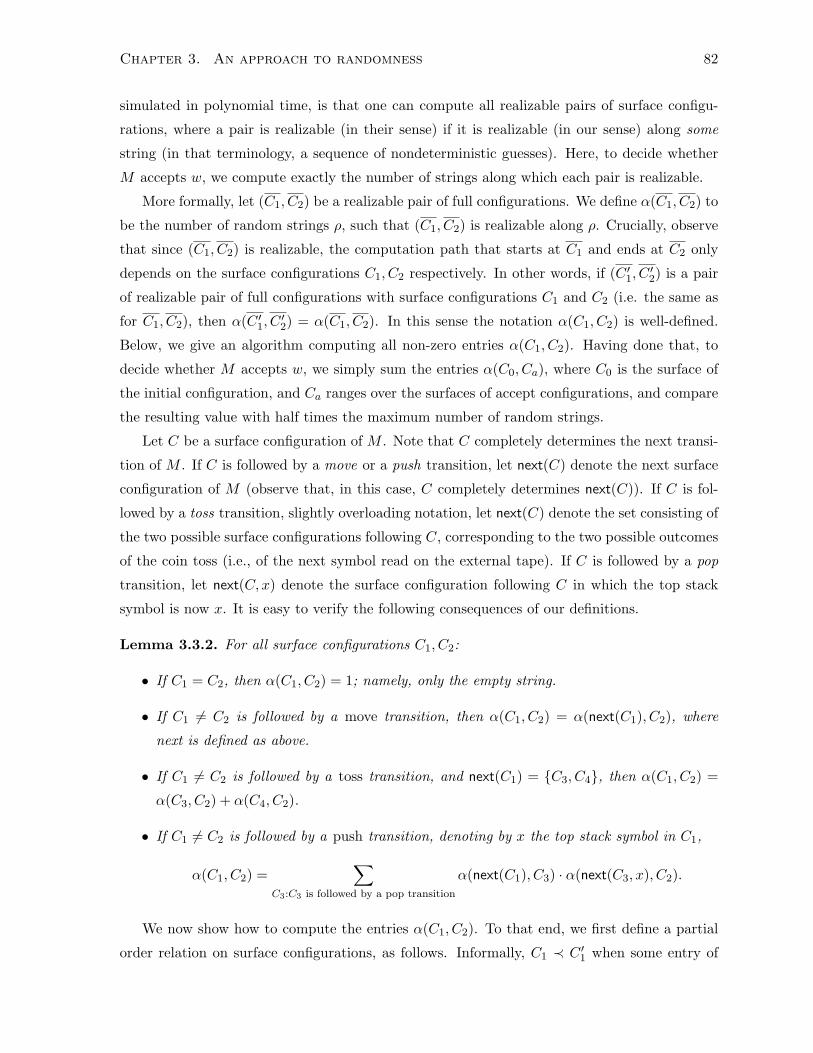
Chapter 3. An approach to randomness 82
simulated in polynomial time, is that one can compute all realizable pairs of surface configu-
rations, where a pair is realizable (in their sense) if it is realizable (in our sense) along some
string (in that terminology, a sequence of nondeterministic guesses). Here, to decide whether
M accepts w, we compute exactly the number of strings along which each pair is realizable.
More formally, let (C1, C2) be a realizable pair of full configurations. We define α(C1, C2) to
be the number of random strings ρ, such that (C1, C2) is realizable along ρ. Crucially, observe
that since (C1, C2) is realizable, the computation path that starts at C1 and ends at C2 only
depends on the surface configurations C1, C2 respectively. In other words, if (C ′1, C′2) is a pair
of realizable pair of full configurations with surface configurations C1 and C2 (i.e. the same as
for C1, C2), then α(C ′1, C′2) = α(C1, C2). In this sense the notation α(C1, C2) is well-defined.
Below, we give an algorithm computing all non-zero entries α(C1, C2). Having done that, to
decide whether M accepts w, we simply sum the entries α(C0, Ca), where C0 is the surface of
the initial configuration, and Ca ranges over the surfaces of accept configurations, and compare
the resulting value with half times the maximum number of random strings.
Let C be a surface configuration of M . Note that C completely determines the next transi-
tion of M . If C is followed by a move or a push transition, let next(C) denote the next surface
configuration of M (observe that, in this case, C completely determines next(C)). If C is fol-
lowed by a toss transition, slightly overloading notation, let next(C) denote the set consisting of
the two possible surface configurations following C, corresponding to the two possible outcomes
of the coin toss (i.e., of the next symbol read on the external tape). If C is followed by a pop
transition, let next(C, x) denote the surface configuration following C in which the top stack
symbol is now x. It is easy to verify the following consequences of our definitions.
Lemma 3.3.2. For all surface configurations C1, C2:
• If C1 = C2, then α(C1, C2) = 1; namely, only the empty string.
• If C1 6= C2 is followed by a move transition, then α(C1, C2) = α(next(C1), C2), where
next is defined as above.
• If C1 6= C2 is followed by a toss transition, and next(C1) = C3, C4, then α(C1, C2) =
α(C3, C2) + α(C4, C2).
• If C1 6= C2 is followed by a push transition, denoting by x the top stack symbol in C1,
α(C1, C2) =∑
C3:C3 is followed by a pop transition
α(next(C1), C3) · α(next(C3, x), C2).
We now show how to compute the entries α(C1, C2). To that end, we first define a partial
order relation on surface configurations, as follows. Informally, C1 ≺ C ′1 when some entry of
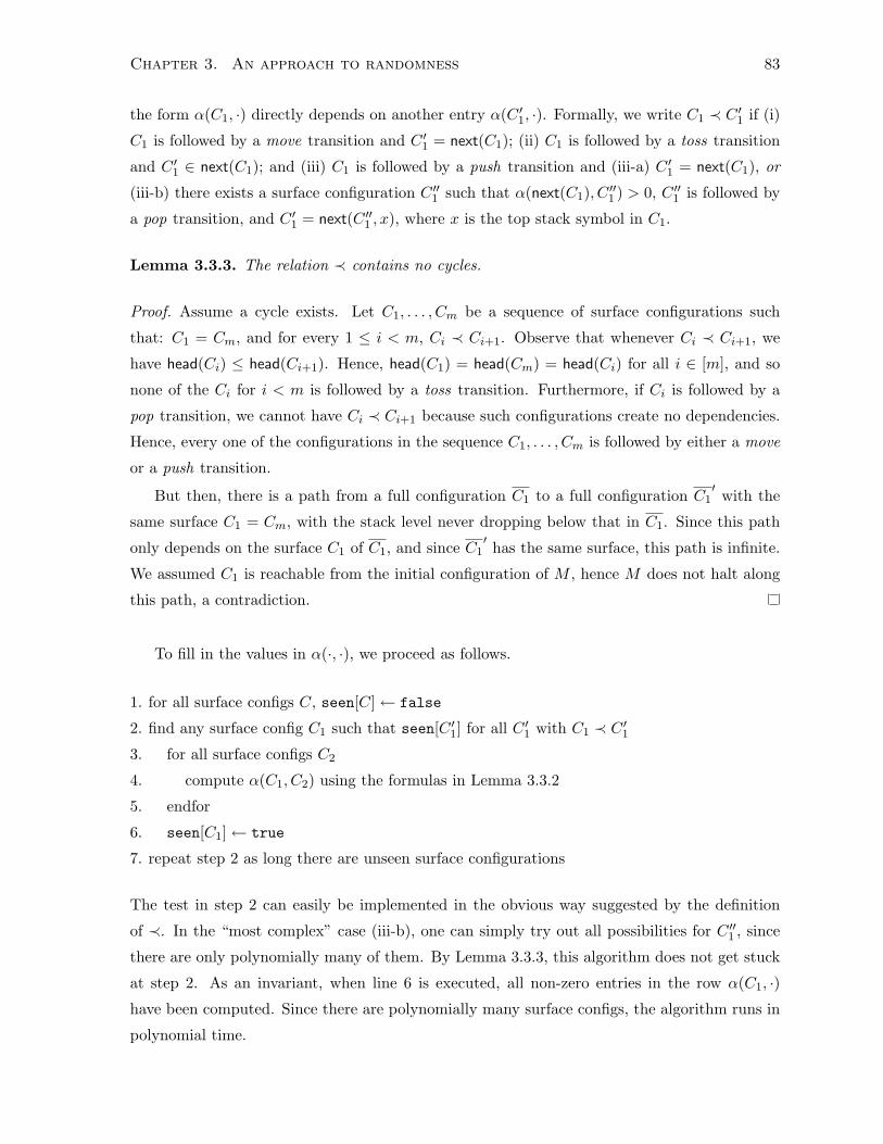
Chapter 3. An approach to randomness 83
the form α(C1, ·) directly depends on another entry α(C ′1, ·). Formally, we write C1 ≺ C ′1 if (i)
C1 is followed by a move transition and C ′1 = next(C1); (ii) C1 is followed by a toss transition
and C ′1 ∈ next(C1); and (iii) C1 is followed by a push transition and (iii-a) C ′1 = next(C1), or
(iii-b) there exists a surface configuration C ′′1 such that α(next(C1), C ′′1 ) > 0, C ′′1 is followed by
a pop transition, and C ′1 = next(C ′′1 , x), where x is the top stack symbol in C1.
Lemma 3.3.3. The relation ≺ contains no cycles.
Proof. Assume a cycle exists. Let C1, . . . , Cm be a sequence of surface configurations such
that: C1 = Cm, and for every 1 ≤ i < m, Ci ≺ Ci+1. Observe that whenever Ci ≺ Ci+1, we
have head(Ci) ≤ head(Ci+1). Hence, head(C1) = head(Cm) = head(Ci) for all i ∈ [m], and so
none of the Ci for i < m is followed by a toss transition. Furthermore, if Ci is followed by a
pop transition, we cannot have Ci ≺ Ci+1 because such configurations create no dependencies.
Hence, every one of the configurations in the sequence C1, . . . , Cm is followed by either a move
or a push transition.
But then, there is a path from a full configuration C1 to a full configuration C1′ with the
same surface C1 = Cm, with the stack level never dropping below that in C1. Since this path
only depends on the surface C1 of C1, and since C1′ has the same surface, this path is infinite.
We assumed C1 is reachable from the initial configuration of M , hence M does not halt along
this path, a contradiction.
To fill in the values in α(·, ·), we proceed as follows.
1. for all surface configs C, seen[C]← false
2. find any surface config C1 such that seen[C ′1] for all C ′1 with C1 ≺ C ′13. for all surface configs C2
4. compute α(C1, C2) using the formulas in Lemma 3.3.2
5. endfor
6. seen[C1]← true
7. repeat step 2 as long there are unseen surface configurations
The test in step 2 can easily be implemented in the obvious way suggested by the definition
of ≺. In the “most complex” case (iii-b), one can simply try out all possibilities for C ′′1 , since
there are only polynomially many of them. By Lemma 3.3.3, this algorithm does not get stuck
at step 2. As an invariant, when line 6 is executed, all non-zero entries in the row α(C1, ·)have been computed. Since there are polynomially many surface configs, the algorithm runs in
polynomial time.
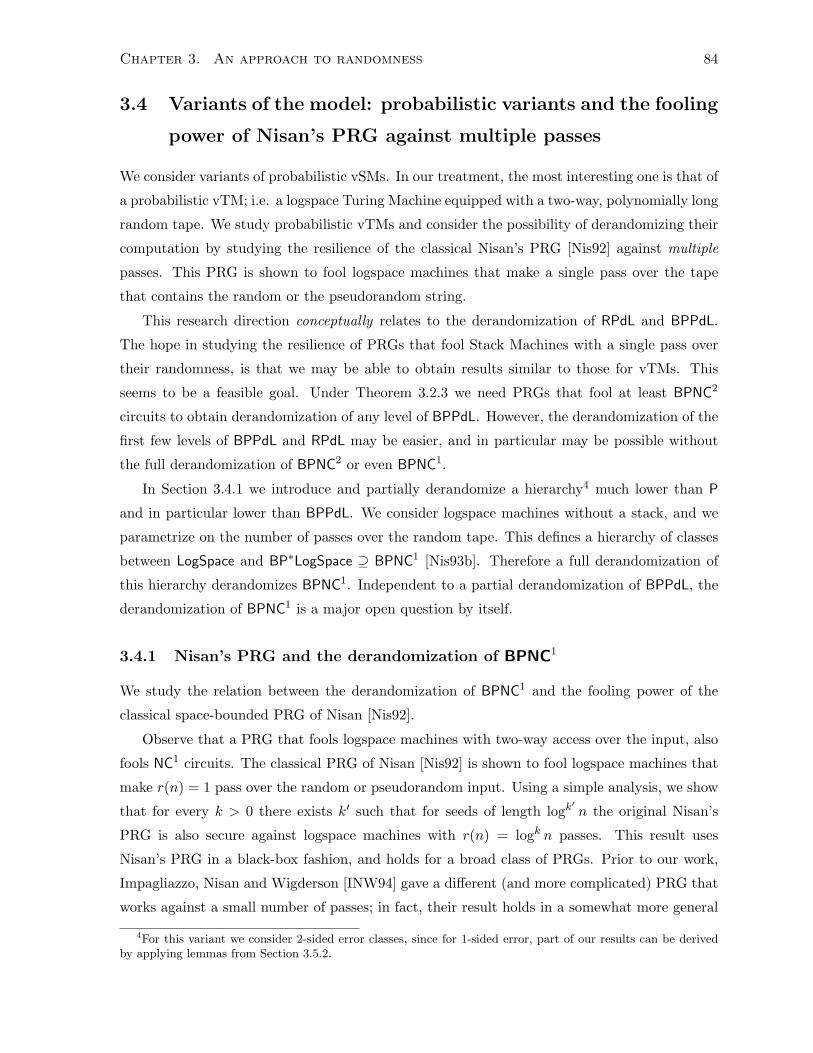
Chapter 3. An approach to randomness 84
3.4 Variants of the model: probabilistic variants and the fooling
power of Nisan’s PRG against multiple passes
We consider variants of probabilistic vSMs. In our treatment, the most interesting one is that of
a probabilistic vTM; i.e. a logspace Turing Machine equipped with a two-way, polynomially long
random tape. We study probabilistic vTMs and consider the possibility of derandomizing their
computation by studying the resilience of the classical Nisan’s PRG [Nis92] against multiple
passes. This PRG is shown to fool logspace machines that make a single pass over the tape
that contains the random or the pseudorandom string.
This research direction conceptually relates to the derandomization of RPdL and BPPdL.
The hope in studying the resilience of PRGs that fool Stack Machines with a single pass over
their randomness, is that we may be able to obtain results similar to those for vTMs. This
seems to be a feasible goal. Under Theorem 3.2.3 we need PRGs that fool at least BPNC2
circuits to obtain derandomization of any level of BPPdL. However, the derandomization of the
first few levels of BPPdL and RPdL may be easier, and in particular may be possible without
the full derandomization of BPNC2 or even BPNC1.
In Section 3.4.1 we introduce and partially derandomize a hierarchy4 much lower than P
and in particular lower than BPPdL. We consider logspace machines without a stack, and we
parametrize on the number of passes over the random tape. This defines a hierarchy of classes
between LogSpace and BP∗LogSpace ⊇ BPNC1 [Nis93b]. Therefore a full derandomization of
this hierarchy derandomizes BPNC1. Independent to a partial derandomization of BPPdL, the
derandomization of BPNC1 is a major open question by itself.
3.4.1 Nisan’s PRG and the derandomization of BPNC1
We study the relation between the derandomization of BPNC1 and the fooling power of the
classical space-bounded PRG of Nisan [Nis92].
Observe that a PRG that fools logspace machines with two-way access over the input, also
fools NC1 circuits. The classical PRG of Nisan [Nis92] is shown to fool logspace machines that
make r(n) = 1 pass over the random or pseudorandom input. Using a simple analysis, we show
that for every k > 0 there exists k′ such that for seeds of length logk′n the original Nisan’s
PRG is also secure against logspace machines with r(n) = logk n passes. This result uses
Nisan’s PRG in a black-box fashion, and holds for a broad class of PRGs. Prior to our work,
Impagliazzo, Nisan and Wigderson [INW94] gave a different (and more complicated) PRG that
works against a small number of passes; in fact, their result holds in a somewhat more general
4For this variant we consider 2-sided error classes, since for 1-sided error, part of our results can be derivedby applying lemmas from Section 3.5.2.
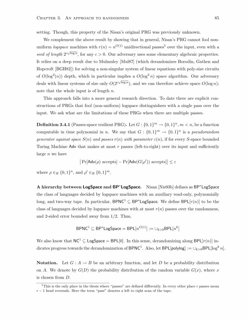
Chapter 3. An approach to randomness 85
setting. Though, this property of the Nisan’s original PRG was previously unknown.
We complement the above result by showing that in general, Nisan’s PRG cannot fool non-
uniform logspace machines with r(n) = nO(1) unidirectional passes5 over the input, even with a
seed of length 2c√
logn, for any c > 0. Our adversary uses some elementary algebraic properties.
It relies on a deep result due to Mulmuley [Mul87] (which derandomizes Borodin, Gathen and
Hopcroft [BGH82]) for solving a non-singular system of linear equations with poly-size circuits
of O(log2(n)) depth, which in particular implies a O(log2 n) space algorithm. Our adversary
deals with linear systems of size only O(2c√
logn), and we can therefore achieve space O(log n);
note that the whole input is of length n.
This approach falls into a more general research direction. To date there are explicit con-
structions of PRGs that fool (non-uniform) logspace distinguishers with a single pass over the
input. We ask what are the limitations of these PRGs when there are multiple passes.
Definition 3.4.1 (Passes-space resilient PRG). LetG : 0, 1m → 0, 1n, m < n, be a function
computable in time polynomial in n. We say that G : 0, 1m → 0, 1n is a pseudorandom
generator against space S(n) and passes r(n) with parameter ε(n), if for every S-space bounded
Turing Machine Adv that makes at most r passes (left-to-right) over its input and sufficiently
large n we have ∣∣Pr[Adv(ρ) accepts]− Pr[Adv(G(ρ′)) accepts]∣∣ ≤ ε
where ρ ∈R 0, 1n, and ρ′ ∈R 0, 1m.
A hierarchy between LogSpace and BP∗LogSpace. Nisan [Nis93b] defines as BP∗LogSpace
the class of languages decided by logspace machines with an auxiliary read-only, polynomially
long, and two-way tape. In particular, BPNC1 ⊆ BP∗LogSpace. We define BPL[r(n)] to be the
class of languages decided by logspace machines with at most r(n) passes over the randomness,
and 2-sided error bounded away from 1/2. Thus,
BPNC1 ⊆ BP∗LogSpace = BPL[nO(1)] := ∪k>0BPL[nk]
We also know that NC1 ⊆ LogSpace = BPL[0]. In this sense, derandomizing along BPL[r(n)] in-
dicates progress towards the derandomization of BPNC1. Also, let BPL[polylog] := ∪k>0BPL[logk n].
Notation. Let G : A → B be an arbitrary function, and let D be a probability distribution
on A. We denote by G(D) the probability distribution of the random variable G(x), where x
is chosen from D.
5This is the only place in the thesis where “passes” are defined differently. In every other place r passes meanr − 1 head reversals. Here the term “pass” denotes a left to right scan of the tape.
Chapter 3. An approach to randomness 86
Let N ≥ 1, and let D be a probability distribution over 0, 1N . For any t ≥ 1, we denote
by Dt the probability distribution over 0, 1Nt obtained by taking t concatenated copies of a
string x that is chosen from D.
Let D1, D2 be probability distributions over a finite set A. We use the notation
‖D1 −D2‖1 =∑x∈A
∣∣∣∣ Pry1∈D1
[y1 = x]− Pry2∈D2
[y2 = x]∣∣∣∣ .
A non-uniform, one-way TM M is equivalent to a family of Finite State Machines (FSMs).
Let Q be a FSM with alphabet 0, 1, and with a designated initial state, and let D be a
probability distribution over 0, 1n. Then, we denote by Q(D) the matrix whose (i, j)-th
entry is the probability getting from state i to state j after reading a string x chosen from D.
For a matrix P ∈ RN×N let ‖P‖1 = maxi∑
j |Pi,j |.
Derandomizing the first polylog levels: BPL[polylog] ⊆ QuasiP
Since we deal with space-bounded machines realized as FSMs, the following definition is stronger
than Definition 3.4.1.
Definition 3.4.2 (Pseudorandom generator against FSMs). Let G : 0, 1m → 0, 1n be
computable in time polynomial in n, and let ε, w > 0. We say that G is a pseudorandom
generator against FSMs for space w with parameter ε if for any FSM Q with 2w states, we have
‖Q(Un)−Q(G(Um))‖1 ≤ ε.
Theorem 3.4.3 (Nisan [Nis92]). There exists c > 0 such that for any N > 0, there exists a
function G : 0, 1N2 → 0, 1N2cN computable in time polynomial in 2cN which is a pseudo-
random generator against FSMs for space cN , with parameter 2−cN .
Instead of considering an adversary as an FSM with multiple passes over the input, it
is convenient to consider a one-way FSM whose input contains multiple copies of the original
input. For a function G : 0, 1m → 0, 1n we define G2 : 0, 1m → 0, 12n, x 7→ G(x)G(x),
where denotes concatenation of strings. The following simple lemma states that Nisan’s PRG
works (with a small loss in the parameter) even if the space-bounded machine is allowed to
make two passes over the random tape.
Lemma 3.4.4. Let G : 0, 1m → 0, 1n be a PRG against FSMs for space 2s with parameter
ε. Then G2 : 0, 1m → 0, 12n is a PRG against FSMs with space s with parameter ε′ = ε·22s.
Proof. Suppose that G2 is not pseudorandom against FSMs of space s with parameter ε′. We
show that G is not a PRG against FSMs for space 2s with parameter ε.
Chapter 3. An approach to randomness 87
Therefore, there exists a FSM with state space 1, . . . , 2s such that
‖Q(G2)−Q(U2n)‖1 > ε′ (3.4.1)
Let 1 be the initial state of Q. For a string x ∈ 0, 1n, and for i, j ∈ 1, . . . , 2s we write
ix−→Q j to denote the event that starting from state i and reading the string x, the FSM Q
ends up to state j. For any i, j ∈ 1, . . . , 2s let
pi,j = Prx∈G
[1 x−→Q i and ix−→Q j]
and
qi,j = Pry∈Un
[1y−→Q i and i
y−→Q j]
From (3.4.1) we have ∑i∈1,...,2s
∑j∈1,...,2s
|pi,j − qi,j | ≥ ‖Q(G2)−Q(U2n)‖1 > ε′
Therefore, there exist i∗, j∗ ∈ 1, . . . , 2s such that
|pi∗,j∗ − qi∗,j∗ | > ε′/22s
Let Q′ be a FSM with state space 1, . . . , 2s × 1, . . . , 2s, and alphabet 0, 1. We define
the transition function of Q′ so that for any b ∈ 0, 1 and for any i, j ∈ 1, . . . , 2s, we have
(i, j) b−→Q′ (i′, j′) iff ib−→Q i
′ and jb−→Q j
′. We set the initial state of Q′ to be (1, i∗). We have
‖Q′(G)−Q′(Un)‖1 =∑
i,j∈1,...,2s
∣∣∣∣ Prx∈G
[(1, i∗) x−→Q′ (i, j)]− Pry∈Un
[(1, i∗)y−→Q′ (i, j)]
∣∣∣∣≥
∣∣∣∣ Prx∈G
[(1, i∗) x−→Q′ (i∗, j∗)]− Pry∈Un
[(1, i∗)y−→Q′ (i∗, j∗)]
∣∣∣∣=
∣∣∣∣ Prx∈G
[1 x−→Q i∗ and i∗
x−→Q j∗]− Pr
y∈Un[1
y−→Q i∗ and i∗
y−→Q j∗]∣∣∣∣
= |pi∗,j∗ − qi∗,j∗ |
> ε′/22s
= ε
Therefore, G is not a PRG against FSMs of space 2s with parameter ε.
Note that every time we apply Lemma 3.4.4 on a PRG G we get a new PRG G′ which is
secure against twice as many passes as G, with slightly worse space and error parameters. By
repeating O(log log n) times, we obtain Theorem 3.4.5 which we restate below.
Theorem 3.4.5. BPL[polylog] ⊆ QuasiP.
Chapter 3. An approach to randomness 88
Breaking Nisan’s PRG with polynomially many passes
Let n be the length of the output of Nisan’s PRG. Fix c > 0 and the seed length to be 2c√
logn.
In Theorem 3.4.3 we stated a corollary of the theorem from [Nis92], by choosing the parameters
appropriately. We used Theorem 3.4.3 to obtain a positive result. However, for breaking
Nisan’s PRG (with polynomially many passes) we consider its general form. Note, that our
adversary overwhelmingly breaks the security properties (stated for one-pass) of Nisan’s PRG.
In particular, for seed length 2c√
logn instead of a 2c′√logn space, c′ > 0, distinguisher we present
a logspace one. Furthermore, we distinguish with probability much bigger than 2−c′√logn.
Let us review the description of Nisan’s PRG.
Let H be a universal family of hash functions h : 0, 1N → 0, 1N , for some N . We are
going to determine all parameters after the description of the PRG. For every integer k ≥ 0
define the generator
Gk : 0, 1N ×Hk → (0, 1N )2k
where Gk is defined recursively as follows:
• G0(x) = x, and
• Gm(x, h1, . . . , hm) = Gm−1(x, h1, . . . , hm−1) Gm−1(hm(x), h1, . . . , hm−1), where de-
notes concatenation of strings.
Nisan shows that such a PRG is secure against FSMs that make a single pass over the input.
He uses an explicit efficiently computable family H of affine functions h : GF (2)N → GF (2)N .
A function h is affine if there is a linear function fh and a b ∈ GF (2)N such that h(x) = fh(x)+b
for all x ∈ GF (2)N . Nisan’s [Nis92] family H has the property that each h ∈ H can be described
in O(N) bits.
Additional terminology and notation. The output of the PRG consists of blocks, each
of which is an N -bit binary string, and it corresponds to evaluating x on some composition
of functions from H. Let hi1,...,il = hi1 . . . hil , where denotes function composition. By
definition, in Gk(x, h1, . . . , hk) each block will be the composition of hi1 hi2 · · · hil evaluated
on x, where i1 < i2 < · · · < ll. By definition, given the output y of the PRG on some x
with family H = h1, . . . , hk, an increasing sequence 〈i1, i2, . . . il〉, ij ∈ 1, . . . , k uniquely
determines the position of hi1,...,il(x) in y.
The parameters. The output length is n = 2kN . Therefore, k = O(log n). For a family
H as in [Nis92], the seed length is O(kN). Therefore, for seed length 2c√
logn we have that
N = O(2c√
logn).
Chapter 3. An approach to randomness 89
The main idea. Suppose that the string y is the output of Nisan’s PRG, withH = h1, . . . , hkthe family of affine functions and some x. We will describe a test that every such y passes, but
almost every string fails to pass. Note that to perform the test we do not need to know the
actual hi. The given 〈i1, . . . , il〉 is sufficient to determine the position of hi1,...,il(x) on y.
Here is a property that our test will use. We treat every block (which is in particular a
binary substring of length N) of y as a vector in GF (2)N . Let y1, . . . , yl be an even number of
blocks in y and h : GF (2)N → GF (2)N an affine function. If y1, . . . , yl are linearly dependent6
then h(y1) + · · ·+ h(yl) = 0. Furthermore, suppose that h := h1 ∈ H and h1 is not used in the
composed functions determining the yi’s. Recall that for every block yi we know the position
of h(yi) on y.
Therefore, the output of Nisan’s PRG y passes the following test: find an even number of
linearly independent blocks y1, . . . , yl indexed by the hi’s where i > 1, and check whether the
sum of the blocks corresponding to h1(yi) evaluate to 0. Observe that to perform this test we
don’t have to know the actual hi’s. We refer to the hi’s just for determining the positions of
the corresponding blocks.
Observe that if y is random then the probability that at least 2 vectors corresponding to
N -bit substrings of y sum up to 0 is 2−N .
The logspace distinguisher. Let y be the input to the distinguisher.
1. Let I1 := 2, 3, . . . , k2, and I2 := k2 + 1, . . . , k. Use I1 and I2 to index block positions.
Let H1 be the first N + 1 blocks indexed by 〈i1, . . . , il〉, 1 < i1 < . . . < il, with ij ∈ I1.
Similarly, we define H2 where the indices are determined using I2. Hence, in both cases
for y (either y is the output of Nisan’s PRG on random H and x, or y is a random string)
we have that (i) H1 ∩H2 = ∅ with probability ≥ 1 − 2−Ω(N), and (ii) each of the sets is
larger than N , which guarantees that the vectors in H1 are linearly dependent, and the
same holds for H2.
2. Use [Mul87] (see below) to find in space O(log n) a set of linearly dependent vectors in
H1: y(1)1 + y
(1)2 + . . .+ y
(1)j1
= 0, and a set of linearly dependent vectors in H2: y(2)1 + y
(2)2 +
. . .+ y(2)j2
= 0. As usual in space-bounded computation, by this we mean that each time
we can (re)compute the indices of the vectors on the input tape.
3. If j1 is even, accept iff∑j1
j=1 αy(1)j
= 0, where αy
(1)j
is the block indexed by the composition
of h1 with the composed functions corresponding to y(1)j . Similarly, if j2 is even. Else, if
both j1 and j2 are odd then j1 + j2 is even, and accept iff∑j1
j=1 αy(1)j
+∑j2
j=1 αy(2)j
= 0.
6For an even l, h(y1) + · · · + h(yl) = fh(y1) + · · · + fh(yl) = fh(y1 + · · · + yl). In particular, y1 + · · · + yl =0 =⇒ h(y1) + · · ·+ h(yl) = 0, since fh is linear.
Chapter 3. An approach to randomness 90
Clearly, if the input is random then the probability that the adversary accepts is 2−Ω(N).
On the other hand, if the input is pseudorandom then with probability at least 1− 2−Ω(N) we
have that (i) H1 ∩H2 = ∅, and (ii) all vectors in H1 ∪H2 are non-zero. Conditioned on these
two events, the adversary accepts with probability 1.
Finding the linear dependencies. Let NonSingular-Equations(n) be the problem of
solving a non-singular n× n system of linear equations [BGH82]. From [Mul87] we have.
Theorem 3.4.6 (Mulmuley [Mul87]). NonSingular-Equations(n) can be computed in the
functional analog of the uniform NC2 (i.e. the circuits can have multiple outputs).
Consider the following procedure. Fix y ∈ H1 and let A be the N ×N matrix with columns
z ∈ H1 − y. If y 6= 0, then every solution of the system Ax = y is non-zero. Since the set
of vectors in H1 is linearly dependent, there exists at least one y such that the system has a
solution. This solution gives us the required set of vectors y(1)1 + . . . + y
(1)j1
= 0. Similarly for
H2.
Recall that NC2 ⊆ DSPACE(log2 n). However, when solving the linear system Ax = y in the
above procedure, the input length is not n, but polynomial in N = O(2c√
logn). Therefore, by
Theorem 3.4.6, the above procedure can be implemented in space O(log n) and thus we obtain
the following theorem. Note that the length of the advice is O(2c√
logn).
Theorem 3.4.7. Let c > 0. There exists k > 0, such that Nisan’s PRG with seed of length
2c(√
logn) is not secure against logspace machines that make nk passes over the input.
3.4.2 The expected number of passes for probabilistic Verifier Stack Ma-
chines
We also consider the variant of probabilistic vSMs where the number of passes is an average-
case resource. For RPdL the number of passes over the random tape is a worst-case resource,
similar to the time-resource in the definition of RP and BPP. We define the hierarchy RPdLE
same as RPdL where each level is defined with respect to the expected number of passes over
the random tape. Contrast this to Randomness Compilers where a similar definition would be
less natural. This shows an intuitive advantage of the vSM model.
Using a simple averaging argument we obtain that the first polynomially many levels of
both hierarchies RPdL and RPdLE coincide. This is a corollary of the following lemma.
Lemma 3.4.8. RPdL[r(n)] ⊆ RPdLE[r(n)] ⊆ RPdL[O(r(n))], where r(n) = nO(1).
The proof of this lemma follows by standard arguments. In particular, for the non-trivial
inclusion, we simulate the machine where the expected number of passes is r(n) say for 4r(n)
steps, and then apply Markov’s inequality.
Chapter 3. An approach to randomness 91
3.5 Variants of the model: non-deterministic variants
We consider two nondeterministic variants of the model. The first is a vSM with a nondeter-
ministic tape. In this case a certain compressibility property of NP-witnesses implies that two
passes over the (nondeterministic) auxiliary tape suffice to do all of NP. The other variant is
vTMs with a nondeterministic tape. In this case we show a tight connection with deciding
width parametrizations of SAT, and in particular with SAT of fixed pathwidth.
3.5.1 NPdL[2] = NP
We show the following theorem. Not surprisingly, this intuitively implies that derandomizing
the second level of the RPdL is non-trivial, in the sense that the boundedness of error is relevant.
Theorem 3.5.1. The non-deterministic hierarchy collapses to level 2. More specifically, NPdL[2] =
NP. Also, NPdL[1] = P.
Proof. NPdL[1] = P follows directly by Theorem 1 p.7 [Coo71].
We show that NPdL[2] = NP. By the NP-completeness of 3-SAT under many-to-one logspace
reductions, it suffices to decide 3-SAT in NPdL[2], since NPdL[2] is closed under logspace reduc-
tions.
We describe a non-deterministic SM for 3-SAT. Let φ be the 3-CNF formula given in
the input, with n variables x1, . . . , xn and m clauses C1, . . . , Cm. Let τ be a truth assignment
identified by the string 〈τ(x1), . . . , τ(xn)〉 and let τR denote the reversed string. Simultaneously,
we: (i) check the truth assignment is a satisfying one; and (ii) check that the external tape is of
the form 〈τ, τR, . . . , τ, τR, τ, τR〉︸ ︷︷ ︸m times
. Associate with the first clause C1 the first copy of the truth
assignment τ , with C2 the second copy τR, and so on up to Cm.
To check (i) we do not use the stack. Verify that τ satisfies C1, τR satisfies C2 and so
on. This verification can be done in one scan over the non-deterministic tape, just using the
logspace worktape.
To check (ii) we use the stack and the worktape as follows. Suppose that the external
memory contains the strings w1, . . . wn−1, wn. In the first scan the machine uses the stack to
verify that w1 = wR2 , . . ., wn−3 = wRn−2, and wn−1 = wRn . When the head reverses it uses
the stack to verify that wn−1 = wRn−2 and so on. Intuitively, we first verify equality between
mutually exclusive pairs and then we “link” them by verifying equality among the pairs.
We remark that a similar argument shows that PPdL[2] = PP.
Chapter 3. An approach to randomness 92
3.5.2 Verifying NP-witnesses with limited access to the witness
Our motivation for studying vTMs with non-deterministic tape goes beyond the study of yet-
another-variant of the vSM model. We aim to understand the complexity of problems in
NP, when the access to the NP-witness is parametrized. In a different direction, we aim to
syntactically characterize the decision complexity of width-parametrizations of SAT. It turns
out that these two are very well related.
Width-parametrizations of SAT are studied as a case of parametrized complexity (cf.
[FG06]). There is an extensive body of work, too large to be cited here (e.g. see [Sze03] for
an older survey). We characterize the complexity of SAT instances with path-decompositions of
width w(n). Although pathwidth is the most restrictive among the studied width-parametrizations
of SAT, the most time-efficient algorithms known for such SAT instances run in time 2Ω(w(n)),
even when the path-decomposition is given in the input. We wish to better understand the
decision complexity of SAT instances of width ω(log n). We provide an exact correspondence
between SATpw[w(n)], the problem of SAT instances with given path decomposition of width
w(n), and NL[r(n)], the class of problems decided by logspace Turing Machines with at most
r(n) passes over the polynomially long nondeterministic tape. In particular, we show that
SATpw[w(n)] is hard for NL[w(n)logn ] under logspace reductions. When NL[w(n)
logn ] is closed under
logspace reductions, which is the case for the most interesting w(n)’s, we show that SATpw[w(n)]
is also complete.
Note that by parametrizing on the number of passes over the non-deterministic tape we
define a hierarchy between NL and NP. We denote by NL[r(n)] the class of sets accepted by
vTMs where the head of the nondeterministic tape is allowed to reverse r(n) − 1 times, i.e.
making r(n) passes. Thus, NL[1] = NL and NL[nO(1)] := ∪c>0NL[nc] = NP. Note that other
than the nondeterministic tape, all other tapes have an unbounded number of reversals, as in
a standard logspace TM.
Motivation for width-parametrizations of SAT. A common way to consider subprob-
lems of SAT is to parametrize the input according to some graph-theoretic width-parameter
measured on a graph associated with the input formula. The incidence graph is a canonical
example of such a graph (see below for a definition). Treewidth, pathwidth, cliquewidth and so
on, are width parameters for CNF instances, extensively studied both in theoretical and empir-
ical research. This line of research gives algorithms (for inputs with restricted parameters) with
running times significantly better than that of exhaustive search. Different parametrizations of
SAT have been studied under different settings, but in general no algorithms faster than 2O(w(n))
are known, even when the width w(n) corresponds to pathwidth, the most restrictive among
the studied width-parameters. We observe that the Exponential Time Hypothesis (ETH), a
Chapter 3. An approach to randomness 93
strong complexity assumption, can be used to obtain lower bounds on the time complexity
of SAT instances of pathwidth ω(log n). One motivating question is whether we can relate
the non-existence of polytime algorithms for such SAT instances with complexity assumptions
weaker than the ETH.
We denote by SATpw[w(n)] the set of satisfiable CNFs with given path decompositions of
width w(n), where n is the input length (definitions given later on in this section). By providing
the path decomposition in the input in some sense we mod-out the difficulty of computing the
pathwidth.
Conjecture. Let w(n) = ω(log n). Then, SATpw[w(n)] 6∈ P.
Conditioned on ETH this conjecture becomes true (see below). ETH [IPZ98] states that
the N variable 3-SAT can’t be solved in time 2o(N). Making further progress seems difficult,
partly because the precise complexity of SATpw[w(n)] is unknown. In [GP08] it is observed that
for k-CNFs with path decompositions of width w(n) the 2O(w(n)) running time can be improved
to nondeterministic space O(w(n)). This improvement is far from an exact characterization,
since NSPACE(w(n)) is believed to contain sets not in NP, if w(n) ∈ ω(log n). We use ele-
mentary techniques to precisely characterize the complexity of SATpw[w(n)] by identifying a
correspondence between two seemingly unrelated concepts.
Regarding our motivating conjecture there are some very interesting works for similar ques-
tions, in particular for treewidth parametrized CSPs and for CLIQUE [FK97, Gro03, Mar07].
Also, understanding the power of vTMs is of independent interest. For example, for which
r(n) > 1 is NL[r(n)] ⊆ P? We relate NL[·] and SATpw[·] in a very strong sense.
Theorem 3.5.2. Let w(n) be constructible in space O(log n). Then, SATpw[w(n)] is complete
for NL[w(n)logn ].
Although, the containment and hardness directions find applications on their own, the
completeness makes sense for classes NL[r(n)] closed under logspace reductions. As we will see
this is the case for the most interesting and useful r(n)’s.
Later on we list “Implications of the main Theorem 3.5.2”. For example, based on the
interplay between SATpw and vTMs we obtain lower bounds on the number of nondeterministic
tape head reversals for vTMs.
Remark 3.5.3. Several details matter for the exact characterization to work. For instance, it is
crucial that the parameter is the number of passes over the nondeterministic tape and not some
other measure of “use” of nondeterminism. Furthermore, the same characterization wouldn’t
work for treewidth, since SATpw[log n] is complete for NL, but we conjecture that the same
problem for treewidth is complete for LOGCFL (one can show containment [GP08]), and it is
thought that NL ( LOGCFL.
Chapter 3. An approach to randomness 94
Definitions, notation, and preliminary results
Let φ be a CNF formula with variables L := x1, . . . , xN and clauses R := C1, . . . , Cm. The
incidence graph of φ is a bipartite graph with bipartization (L,R), and there is an edge between
a variable-vertex xi ∈ L and a clause-vertex Cj ∈ R, iff xi appears (signed) in Cj . Path and tree
decompositions are defined over arbitrary graphs as follows. A tree decomposition of a graph
G = (V,E) is the pair τ := (Xi : i ∈ I, T = (I, F )), such that Xi ⊆ V , ∪Xi = V , T is a tree
such that: (i) for every u, v ∈ E there exists i ∈ I such that u, v ∈ Xi, (ii) for every u ∈ Vlet Xi1 , . . . , Xik be the collection of all sets containing u, then the subgraph of T induced by
i1, . . . , ik ∈ I is connected (i.e. it is a tree). The treewidth of G is the minimum width over all
decompositions, where the width of a decomposition is maxi |Xi| − 1. By restricting the tree T
to a path we define the path decomposition, and the pathwidth of G. It is well-known that for a
graph G, tw(G) ≤ pw(G) ≤ (log |V |)tw(G). Finally, we consider ordered k-CNFs Φ each being
a sequence of clauses each consisting of at most k literals. For the given ordering the distance
of a variable x is the index of the clause of the last appearance of x minus the first appearance
of x. The diameter of Φ, diam(Φ) is the maximum distance over its variables. The relevant
computational problems are given below.
Conventions. All reductions are many-to-one and logspace. As usual we denote by n the length
of the input. N is the number of variables in a CNF and M the number of clauses. All widths
are functions of n. We only consider non-decreasing functions w, r : Z+ → Z+ constructible in
logarithmic space.
Problem: SATpw[w(n)]
Input: A CNF formula φ together with a path decomposition of the incidence graph of width
≤ w(n).
Output: Is φ satisfiable?
Problem: SATdiam[w(n)]
Input: An ordered CNF formula Φ where diam(Φ) ≤ w(n).
Output: Is Φ satisfiable?
These problems are inter-reducible within logspace (see Lemma 3.5.4). Usually, we consider
constant clause size CNFs for SATdiam, and arbitrary CNFs for our central problem SATpw.
Lemma 3.5.4. SATdiam[w(n)], SATpw[w(n)], 3-SATpw[w(n)], and SATpw[cw(n)], c > 0 are
inter-reducible.
Chapter 3. An approach to randomness 95
In [GP08] it is shown that 3-SATpw[w(n)] ∈ NSPACE(w(n)), and that 3-SATpw[w(n)] and 3-
SATdiam[w(n)] are logspace reducible to each other. Also, Lemma 3.5.14 states that SATpw[w(n)]
is reducible to 3-SATpw[w(n)]. The proof of Lemma 3.5.14 is given after the “Implications of
the main Theorem 3.5.2”. The above Lemma 3.5.4 follows by [GP08], Lemma 3.5.14, and by
padding; where by padding we mean that we extend a propositional formula by adding new
clauses each of which contains a single, fresh variable.
Remark 3.5.5. Lemma 3.5.4 is somewhat interesting since there is a family of 3-CNFs where
every variable appears only a constant number of times, the formulas are of pathwidth O(log n)
and every ordering of the clauses has diameter Ω( nlogn) [GP08]. This combinatorial exponential
gap is being smoothed out through logspace transformations.
We conclude this part with a useful consequence of the Exponential Time Hypothesis (ETH).
Recall that ETH states that the N -variable 3-SAT cannot be solved in time 2o(N).
Lemma 3.5.6. Let w(n) = ω(log n). If ETH holds then 3-SATpw[w(n)] 6∈ P.
Proof. Suppose that there is a polytime algorithm for SATpw[w(n)]. Since for 3-CNFs, M =
Θ(n log n) there is an (also logspace constructible) superlogarithmic function on the number
of clauses, w′(M) = ω(logM), where there is polytime algorithm A that solves instances of
pathwidth w′(M). Given a 3-CNF φ we decide its satisfiability as follows. Pad the formula
with single-fresh-variable clauses such that for the number of clauses M ′ of the new formula,
we have w′(M ′) ≥ M . Thus, we construct φ′ using 2o(M) new clauses, and the obvious path
decomposition of φ′ is of width ≤ w′(M ′). Hence, A decides satisfiability in time 2o(M), which
by the Sparsification Lemma7 [IPZ98] implies an 2o(N) algorithm, contradicting ETH.
Here is a simple but very interesting implication of the above.
Theorem 3.5.8. PolyLogSpace∩NP 6⊆ P, unless the ETH fails. Furthermore, there exists ε > 0
such that 3-SATpw[logε n] ∈ PolyLogSpace ∩ NP and 3-SATpw[logε n] /∈ P, unless the ETH fails.
Proof. From [GP08] we have that 3-SATpw[log2 n] ∈ NSPACE(log2 n) ⊆ DSPACE(log4 n). By
Lemma 3.5.6 we have that 3-SATpw[log2 n] 6∈ P, unless ETH fails.
7The precise statement of the Sparsification Lemma requires background on notation and definitions notnecessary in our exposition. We will make use of the following corollary of the Sparsification Lemma [IPZ98].
Corollary 3.5.7 ([IPZ98]). Let N,M denote the number of variables and clauses of k-CNF formulas, for anarbitrary fixed constant k ∈ Z. If there exists an algorithm A that solves k-SAT in time 2o(M) then there existsan algorithm A′ that solves k-SAT in time 2o(N).
Chapter 3. An approach to randomness 96
Implications of the main Theorem 3.5.2
The main result for non-deterministic vTMs is Theorem 3.5.2. There are a number of conse-
quences of the containment (Lemma 3.5.15) and hardness (Lemma 3.5.16) directions of this
theorem.
Let us begin with Corollary 3.5.9, which follows by the containment and hardness of Theorem
3.5.2, Lemma 3.5.4, and the NSPACE(w(n)) algorithm for 3-SATdiam[w(n)] given in [GP08].
Corollary 3.5.9. (i) NL[r(n)] = NL[cr(n)], c > 0, and (ii) NL[r(n)] ⊆ NSPACE(r(n) log n).
Proof.
(i) The non-trivial inclusion NL[cr(n)] ⊆ NL[r(n)] is a corollary of the reduction (algorithm) in
the proof of Lemma 3.5.16.
(ii) Let L ∈ NL[r(n)]. By Theorem 3.5.2 L reduces to 3-SATdiam[r(n) log n]. By the algorithm
in [GP08] we conclude that L ∈ NSPACE(r(n) log n).
Corollary 3.5.9 immediately implies the following.
Corollary 3.5.10. NL[r(n)] ⊆ NP ∩ NSPACE(r(n) log n). In particular,
NL[polylog] := ∪k>0NL[logk n] ⊆ NP ∩ PolyLogSpace.
Here are some further implications of Corollary 3.5.9.
As mentioned, the most interesting cases for w(n) are those where NL[w(n)/ log n] is closed
under logspace reductions; e.g. NL[1],NL[log log n],NL[logk n]. The closure under logspace
reductions is immediate by Corollary 3.5.9, which also implies that a constant number of passes
over the nondeterministic tape can’t get us outside NL.
Corollary 3.5.11. NL[O(1)] := ∪∞i=1NL[i] = NL
Since NL[O(1)] = NL and NL[nO(1)] = NP, it is natural to ask what is the smallest r(n) such
that NL[r(n)] ⊇ P. Under a widely believed complexity assumption, Corollary 3.5.9 implies
that it is not possible to capture P before NP.
Corollary 3.5.12. There does not exist k > 0 such that NL[nk] ⊇ P, unless P ⊆ DSPACE(nk′),
for some k′ ∈ Z+.
It follows by Corollary 3.5.9 and Theorem 3.5.2 that there are r(n)’s where NL[r(n)] is not
closed under logspace reductions, modulo complexity assumptions. For example, if NL[nε] is
closed under logspace reductions then NP ⊆ NL[nε] ⊆ DSPACE(nε′).
A perhaps surprising consequence of the relation between SATpw[·] and NL[·] is Corollary
3.5.13, which follows by the containment direction of Theorem 3.5.2 and Lemma 3.5.6.
Chapter 3. An approach to randomness 97
Corollary 3.5.13. Let r(n) = ω(1). If ETH holds then NL[r(n)] 6⊆ P.
An example of an L in Corollary 3.5.13 is 3-SATpw[ω(log n)] (note that Lemma 3.5.15 also
holds for 3-SATpw[w(n)]).
Observe that we can get Theorem 3.5.8 directly from Corollaries 3.5.13 and 3.5.10. However,
we believe that Corollary 3.5.13 is strictly stronger than Theorem 3.5.8, since we conjecture
that NL[polylog] ( NP ∩ PolyLogSpace.
Proof of Main Theorem and Lemma 3.5.14
Lemma 3.5.4 states that 3-SATdiam and SATpw are inter-reducible, and thus Lemmas 3.5.15
and 3.5.16 imply Theorem 3.5.2. Lemma 3.5.14 allows us to restrict to 3-CNFs, and thus to
conclude Lemma 3.5.4.
Lemma 3.5.14. SATpw[w(n)] is reducible to 3-SATpw[3w(n)].
Proof. Fix 3-CNF Φ of size n, and fix a path decomposition P = 〈X1, X2, . . . , Xα〉 of width
≤ w(n). Let C = l1, . . . , lk be a clause of Φ, and assume that l1, . . . , lk respects the or-
dering of the variables in P . We introduce new variables y1, . . . , yk−1, and note that a truth
assignment to the old variables satisfies C iff some extension to the new variables satisfies all
l1,¬y1, y1, l2,¬y2, . . . , yk−2, lk−1,¬yk−1, yk−1, lk.Consider the smallest s such that C appears inXs together with some variable which appears
in C. Remove C from every Xs′ , where s′ < s.
Let m ≥ s and let Xm contain clause C, and say that the literals li+1, . . . , li+km are the
literals of C whose variables are in Xm and they are not in any earlier Xm′ that contains C.
Case km = 0: in this case all variables for C that are also in Xm have already appeared in
some Xm′ , m′ < m (in fact, since it’s a path decomposition they appear in Xm−1). Then, we
just add to Xm the last yk′ corresponding to C which appears in Xm−1.
Case km > 0: replace Xm by the subpath X1m, . . . , X
kmm where Xj
m is obtained from Xm by
removing C, adding the new variables from the new clause containing li+j , and adding that
new clause as well.
It is not hard to verify that the following properties of the above transformation.
• Because of the rule that we only do the construction of the second case when we have
newly appearing literals, this means that the final path decomposition will have length
a polynomial in α and w(n). Let us give an outline of an argument showing that this is
true. Consider an Xm in the original P . Think of Xm as being the root of a leaf-ordered
tree which represents the splittings of the initial Xm. The (ordered) leaves of the tree
Chapter 3. An approach to randomness 98
correspond to what Xm will be replaced with; i.e. this tree is induced by the “splittings”
that happen because of the “case km > 0”. Then, since we are not splitting unless we
have new literals we observe that this tree grows in depth along its leftmost path and at
each level we have O(w(n)) nodes.
• It is easy to see that given the index of an Xj in the output and a clause C or a variable
x, we can determine in logspace whether C ∈ Xj or x ∈ Xj .
• This transformation results in a valid path decomposition of width ≤ 3w(n).
Note that the resulting formula is satisfiable iff Φ is satisfiable, and the theorem follows by
padding.
Lemma 3.5.15. 3-SATdiam[w(n)] ∈ NL[w(n)logn ], for w(n) = Ω(logn).
Proof. Let Φ be an ordered 3-CNF formula of size n and diameter ≤ w(n). We now present
a nondeterministic logspace algorithm that in each pass over the nondeterministic tape verifies
that nw(n) log n new clauses are satisfied. Hence, Φ is covered in ≤ w(n)
logn passes.
Consider an ordering of the variables of (the clause-ordered) Φ consistent with the ordering
of the clauses. We view the nondeterministic tape as containing a truth assignment, where the
i-th bit of the tape is the truth value of the i-th variable. By definition of diameter, if the j-th
clause in the input has a variable which corresponds to the i-th bit on the nondeterministic
tape, then the (j + w(n))-th clause contains only variables with index ≥ i. For simplicity of
presentation suppose that all divisions are for divisible integers. Partition the ordered clauses
into consecutive blocks each containing log n clauses. The algorithm is iterative, and in each
iteration it deals with exactly one such block which we call “effective block”. Reserve space for
a log n bit vector on the worktape. Each bit of this vector is associated with a clause in the
“effective block”. That is, the input tape is partitioned in blocks b1, b2, . . . , bn/ logn. We define
the distance of two blocks to be the number of clauses between them. Two blocks of distance at
least w(n) do not share any variables. Partition the input tape further into super-blocks, each
of size w(n). That is, we have nw(n) super-blocks each containing α := w(n)
logn blocks. That is,
the blocks can be re-indexed as follows: b1,1, b1,2, . . . , b1,α, b2,1, . . . , b2,α, . . . , bn/w(n),α. Iteratively
make passes over the nondeterministic tape, where in each pass nw(n) blocks are verified to be
satisfiable, as follows.
In the odd numbered passes the nondeterministic head scans from the left to the right
end of the nondeterministic tape, and symmetrically for the even numbered ones. We present
the algorithm for an odd numbered iteration; symmetrically the algorithm works for the even
numbered one. In the i-th iteration we verify the satisfiability of bj,i’s, j = 1, 2, . . . , nw(n) . Start
moving the head on the nondeterministic tape from left to right until we encounter the first
Chapter 3. An approach to randomness 99
variable x that appears in b1,i. Check which (if any) clauses of b1,i are satisfied by x and record
this on the corresponding bits on the reserved log n bit vector on the worktape. Continue this
way until the last variable in the block is read. If the reserved space shows that there is a
clause not satisfied then reject. Else, the nondeterministic head has not read yet any variable
from b2,i. Move the nondeterministic head further and repeat for b2,i as for b1,i; similarly, for
b3,i, . . . , bn/w(n),i.
This algorithm is well-defined since the truth values for the verification they are located at
most w(n) to the left and w(n) to the right of each block. The correctness of this logspace
algorithm is transparent in its description.
An easy modification of the above algorithm makes the lemma true for 3-SATpw[w(n)].
Lemma 3.5.16. 3-SATdiam[w(n)] is hard for NL[w(n)logn ], w(n) = Ω(logn).
Proof. Let r(n) = w(n)logn . Since w(n) is computable in space O(log n), r(n) is also logspace
computable. Fix arbitrary L ∈ NL[r(n)] and let M be a 1-tape logspace vTM accepting L,
which makes r(n) passes over its nondeterministic tape, and is standardized as follows.
(i) M has a unique accepting configuration, (ii) the input head movement of M is oblivious
(meaning that the position of the head is a function of the time step for the given input
length), (iii) M is oblivious in the nondeterministic head movement and in fact it moves the
nondeterministic head in each step in a left to right end (and right to left end) fashion. We
can easily achieve (i), (ii) and make the nondeterministic head move oblivious by slowing down
the computation. In particular, it is easy to make the nondeterministic head stay-put for a
polynomial number of steps p(n) in between moves, and make it move from the left to the right
end of the polynomially q(n)-long tape and back. To standardize the machine to satisfy (iii)
we proceed as follows. Construct a nondeterministic logspace TM verifying in a single pass
whether its nondeterministic tape is of the form b1b1 . . . b1︸ ︷︷ ︸p(n)times
b2b2 . . . b2︸ ︷︷ ︸p(n)times
. . . bq(n)bq(n) . . . bq(n)︸ ︷︷ ︸p(n)times
and
reject if it is not. Composing this logspace machine with the previously standardized logspace
machine we obtain a vTM M for L, satisfying properties (i), (ii), and (iii). On an input of
length n, our standardize TM makes polynomially many t(n) steps.
The hardness follows by modifying the construction in Cook’s theorem for the NP-completeness
of SAT (cf. [DK00] pp. 48-50). For simplicity, we initially deal only with the case where the
number of passes r(n) = 1.
Case r(n) = 1: Let x be an input of length n. We wish to construct an ordered 3-CNF formula
Φ of diameter O(log n) (which by padding is sufficient), such that Φ is satisfiable iff the M
accepts x. We define a configuration γ to be a string which is the concatenation of the strings:
(i) the O(log n) symbols of the worktape, encoding the worktape symbol which the head is on
Chapter 3. An approach to randomness 100
by a special symbol, (ii) the state of M , and (iii) the value of the nondeterministic bit at the
current position in the nondeterministic tape.
For our (standardized) vTM we wish to check whether there exists a sequence of config-
urations γ1 ` γ2 ` . . . ` γt(n), where γ1 is the initial configuration on x, and γt(n) is the
accepting configuration. Our formula will have variables yi,j,α; we will enforce the constraints
that yi,j,α = 1 iff symbol at position j of the configuration at step i is α. We first express
in the usual way that γ1 is the initial configuration. The main technical part is to enforce for
i = 1, . . . , t(n)−1 that γi ` γi+1. We can do this in the usual way, noting that the j-th symbol of
γi+1 only depends on a constant number of symbols of γi, since (by obliviousness) the position
read by the input head is determined by i. It is also important to realize that we do not need
to encode any constraint on the bit read on the nondeterministic tape since a new bit is read
at each step, and since r(n) = 1 no bit is ever reread. Lastly, we express in the usual way that
γt(n) is the accepting configuration. To see that our ordered formula is of diameter O(log n),
the main point is that the subformula needed to express γi ` γi+1 has O(log n) 3-literal clauses
and uses only those variables associated with γi and γi+1; diameter O(log n) comes from the
fact that we encode both γi ` γi+1 and γi+1 ` γi+2.
Case arbitrary r(n): If we perform the above reduction exactly as stated for r(n) > 1 we
do not have a valid reduction, since we must enforce consistency between the different time
steps in which the same nondeterministic bit is visited. If we modify the above construction
such that we reserve the same variable name for the same nondeterministic bit, then this
results in a formula of diameter nΩ(1). Instead, we will always use the same variable name
for the k-th nondeterministic bit, and we will write together all the subformulas describing
those r(n) transitions where the nondeterministic head moves between the k-th and (k + 1)-th
position (in either direction). We do this for k = 1, . . . , z(n) each time creating a subformula
of diameter O(r(n) log n), where z(n) is the polynomial length of the nondeterministic tape.
This can also be expressed in a diagram, where we reorder the configurations denoting by
γpass,symbol the configuration when the nondeterministic head does the number pass scan over
the nondeterministic tape and it currently is at position symbol. Then, the computation starts
by γ1,1 ` γ1,2 ` . . . ` γ1,z(n) and the next configuration is γ2,z(n) since in the second pass the
nondeterministic head moves from the right to the left end.
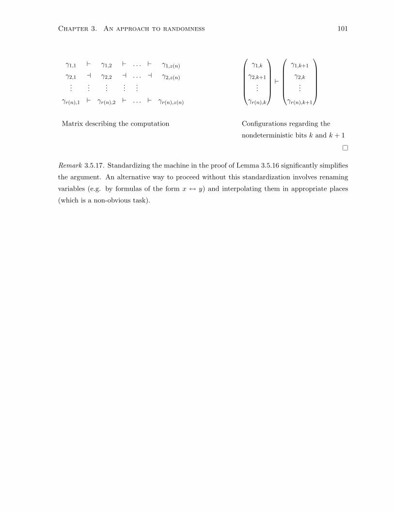
Chapter 3. An approach to randomness 101
γ1,1 ` γ1,2 ` . . . ` γ1,z(n)
γ2,1 a γ2,2 a . . . a γ2,z(n)
......
......
...
γr(n),1 ` γr(n),2 ` . . . ` γr(n),z(n)
γ1,k
γ2,k+1
...
γr(n),k
`
γ1,k+1
γ2,k
...
γr(n),k+1
Matrix describing the computation Configurations regarding the
nondeterministic bits k and k + 1
Remark 3.5.17. Standardizing the machine in the proof of Lemma 3.5.16 significantly simplifies
the argument. An alternative way to proceed without this standardization involves renaming
variables (e.g. by formulas of the form x ↔ y) and interpolating them in appropriate places
(which is a non-obvious task).
Chapter 4
An approach to lower bounds
We show a simultaneous nΩ(1) lower bound in the number of passes over the input tape and
the space of a Stack Machine computing a problem in NC. This is the first lower bound of this
type. Its novelty is technical and conceptual. Conceptually, it falls in our framework of proving
lower bounds - aiming to circuit lower bounds for languages1 in NC in a way orthogonal to
previous approaches. Technically, this is the first lower bound for a streaming model which has
an additional unbounded, read/write memory, restricted to be a stack. By unbounded we mean
that we do not charge for accessing the stack. The argument is a Communication Complexity
reduction from inner product, in the two-player model, to the computation of a Stack Machine
that solves a variant of inner product (a special case of P-Eval). As a side result we obtain a
polynomial separation between a streaming model with a stack where the passes on the external
tape are unidirectional, and a streaming model with a stack where the head can reverse direction
- i.e. similar to the very recent work of Magniez, Mathieu and Nayak [MMN10].
In this chapter we include only the technical developments for the lower bound. For moti-
vation and discussion see Section 1.3. In Section 4.1 we give necessary definitions and notation.
In Section 4.2 we discuss the technical difficulty and the main issues in proving the lower bound
for Stack Machines. We also provide a comparison and show machine-model separation between
this and previous work. The remaining three sections regard the proof of Theorem 4.3.1. In
Section 4.3 we give an outline of the proof, and in Section 4.4 we list the main lemmas, and we
outline their proofs through examples, remarks, and intuitive explanations. We conclude with
the actual proof in Section 4.5.
4.1 Definitions and preliminaries
1Recall that logspace bounded Stack Machines with a single pass over the input can even compute problemsin P− NC (unless exp = PSPACE).
102
Chapter 4. An approach to lower bounds 103
Communication Complexity. We consider the standard two-player Communication Com-
plexity model, where each of the two players receives n bits, and they communicate to compute
a boolean function f : 0, 12n → 0, 1. The resource we measure is the number of commu-
nicated bits. Communication is being done through a shared blackboard (this generalizes to
the p-player Number In Hand model). Deterministic protocols are always correct. For random-
ized protocols the model is extended with shared randomness and we require correctness with
probability at least 2/3. For a function f we denote by D(f) the cost of the best deterministic
protocol, and by R(f) the cost of the best randomized protocol over all inputs and random
strings. For a detailed description of the model see e.g. [KN97].
In chapters 4 and 5 we consider the following functions for which we are interested in their
communication complexity. For a family of functions F , we denote by F2, player’s input size = F2,n
the corresponding function for inputs of size n given to each of the 2 players. The constant 2
denotes the number of players - our model is a special case of the p-player Number In Hand
model. We insist in denoting the number of players as a reminder that the input length is 2n.
When no confusion arises we write F instead of F2,n, and vice-versa.
Here is some initial notation. For a function f : 0, 12n → 0, 1 we use the notation
f(x1, x2), where |xi| = n to denote that Player-i gets input xi. For a string y ∈ 0, 1k we
denote by supp(y) ⊆ 1, . . . , k the set of non-zero indices of y. When necessary we identify
subsets of 1, . . . , k by the support of strings in 0, 1k.
• Inner product : IPF2,n : F2n → F, is the standard inner product over the field F.
• String equality : Equal2,n : 0, 12n → 0, 1, where Equal2,n(x1, x2) = 1 iff x1 = x2.
• Set intersection: SetInt2,n : 0, 12n → 0, 1, where SetInt2,n(x1, x2) = 1 iff supp(x1)∩supp(x2) 6= ∅.
Here are the Communication Complexity lower bounds we use in this and the next chapter.
For a restricted, promise version of SetInt2,n [CKS03] shows in the case of 2 players a linear
lower bound for the randomized complexity. Therefore, R(SetInt2,n) = Ω(n). A simple
reduction from this promise version to inner product over arbitrary F, shows that R(IPF2,n) =
Ω(n). Also, it is well-known (e.g. [KN97]) that D(Equal2,n) ≥ n−1. For clarity of presentation
we restrict to the case where F = GF(2). However, our results hold for every F with an efficient
encoding.
Lift-permute-combine. Our lower bound is for a variant of inner product, which is again an
“inner product problem” where the input is presented in a special way. To that end, during the
reduction the players construct a lifting of the original inner product instance, by constructing
Chapter 4. An approach to lower bounds 104
m instances of IP which they permute and combine appropriately. We introduce notation for
the concept of lift-permute-combine in more generality.
Definition 4.1.1. Consider a base function f : 0, 12N → 0, 1. In the communication
complexity model Player-i gets xi, from an input (x1, x2) ∈ 0, 12N . We denote by Sym(m) the
symmetric group on 1, 2, . . . ,m. Let π ∈ Sym(m), for some parameters N and m := m(N).
The (2mN)-bit function f⊕,π : 0, 12mN → 0, 1 is defined on input x = (x1, x2) ∈ 0, 12mN ,
where xi = (xi,1, . . . , xi,m) ∈ 0, 1Nm, where each |xi,j | = N , i = 1, 2, j = 1, . . . ,m , as follows:
f⊕,π(x) =⊕m
j=1 f(x[j],π), where x[j],π = (x1,j , x2,π(j)). When no confusion arises instead of
x[j],π we write x[j].
Note that in a more general form of this definition, instead of ⊕ one could have used some
other combiner function. Observe that when f = IP2,N then the lifting of an inner product
instance is by definition an inner product instance, where the input is presented in a permuted
way.
Notational remark. Observe that given N, π, n = mN the notation(IPF
2,N
)⊕,π determines
each of the following parameters: N,m, n, since π ∈ Sym(m).
Sortedness. Due to the bidirectional head-move our argument relies on permutations π of
small sortedness. The sortedness of a permutation π on 1, . . . ,m is the maximum length over
all increasing and decreasing subsequences of 〈π(1), . . . , π(m)〉. By e.g. [ES35] it is known that√m < sortedness(π), and that there exists π such that sortedness(π) = O(
√m).
Here are some conventions and additional notation. From this point we assume that for every
m the permutation π is such that sortedness(π) = O(√m). Let d = O(r(2mN) log(2r(2mN))/
√m).
In what follows the choice of r and m will be such that r(2mN) log(2r(2mN)) = o(√m).
Machine models. We consider Stack Machines, parametrized on the number of passes over
their input, as opposed to Chapter 3 where we parametrized over the auxiliary tape. Our main
lower bound holds for the more general model of randomized, non-uniform Stack Machines.
A randomized Stack Machine is a Stack Machine that flips coins (not to be confused with
the vSMs with an auxiliary random tape of the previous section). A non-uniform, s(n) space-
bounded Stack Machine can be identified by a family of two-way finite state machines each
with 2O(s(n)) states for input of length n. We write (r, s)-SM to denote an s(n) space-bounded
Stack Machine that makes at most r(n) passes over its input. We also write (r, s, t)-streaming
algorithm to denote a Turing Machine with workspace s(n) (on which we do not count head-
reversals), it has at most t external tapes, and it makes in total at most r(n) passes over its
external tapes.
Chapter 4. An approach to lower bounds 105
4.2 Motivation and comparison to previous work
4.2.1 Warm-up: a streaming lower bound for IP
The following example demonstrates a technically straightforward application of Communica-
tion Complexity to streaming lower bounds. This is the only section of this chapter where we
consider space-bounded Turing Machines without a stack. A corollary of Lemma 4.2.1 is that
a logspace bounded Turing Machine requires nΩ(1) passes over the input to compute IP2,n.
Technically, we proceed by reducing IP to the computation of a space-bounded TM.
Lemma 4.2.1. Let M be an s(n)-space bounded Turing Machine correct for IP2,n. Then, M
requires Ω( ns(n)) passes over the input to solve IP2,n. Similarly, for SetInt2,n.
Proof. Consider IP2,n. This is a standard argument where we construct a two-player Commu-
nication Complexity protocol using the computation of M . Let n ∈ Z+. Player-1 gets input
x ∈ 0, 1n and Player-2 y ∈ 0, 1n, for the inner product 〈x, y〉. The protocol proceeds in
rounds, where in each round the two players alternate as follows. Player-1 simulates M up until
the point where the head crosses to the y part of the input. Note that the configuration of the
machine is O(s(n)) bits long. Player-1 sends the O(s(n)) bits to Player-2 who continues the
simulation until the input head crosses back to the x part of the input. Then, Player-2 sends
the O(s(n)) bits to Player-1, and the protocol continues with the next round. The head crosses
the middle of the tape at most r(n) times. By the lower bound of IP2,n we know that every
protocol requires Ω(n) bits and thus r(n) = Ω(n/s(n)).
Similarly for SetInt2,n.
What changes in presence of an unbounded stack? When we add a stack, unbounded
in the sense that we do not charge passes over the stack, the above argument fails dramatically.
1. IP2,n can be solved with two passes (i.e. one head reversal). Consider a Stack Machine M
that on input x, y works as follows. In the first pass it pushes x to the stack. That is, at
the end of the first pass the stack contains xR (the string x reversed). In the second pass
the head moves from the right end to the left; i.e. during this move it reads yR. Hence, on
the second pass M pops the stack symbols one by one and it computes 〈xR, yR〉 = 〈x, r〉.
2. The configuration of the machine is too big. It is not only the case that IP2,n cannot be
an example for a lower bound based on the proof template of Lemma 4.2.1. Rather, for
every problem Π the above technique fails. The reason is that the configuration of the
SM is much bigger than O(s(n)), since the stack context can be polynomially large. In
other words, no lower bound is possible using this proof technique.
Chapter 4. An approach to lower bounds 106
4.2.2 Stack Machines compared to other streaming models
Our main technical contribution deals with the issue mentioned in the previous section. In
the literature the basic streaming model [AMS96] has been extended in several ways, e.g.
[GS05, BHN08]. It is reasonable to ask whether lower bounds for Stack Machines can be derived
from streaming lower bounds on machines with multiple external tapes. We can think of two
ways to “derive” lower bounds for Stack Machines from previous streaming lower bounds. The
first is by simulating a Stack Machine with the streaming model with multiple tapes. The second
is conceptual, and it refers to modifying existing proofs. We answer the first interpretation of
the question in the negative. As for the second, we give strong technical evidence that no such
modification is possible in an obvious way.
Comparison of computational models. Is it possible to perform useful computation using
the stack without moving the input head? Intuitively, the proof of the following lemma is related
to a positive answer to this question.
Lemma 4.2.2 (The power of one-way SMs). Let m ∈ Z+. There exists L ∈ P such that (i)
there is a SM deciding L with one pass over the input, and (ii) every TM M with a logspace
work tape (on which we don’t count passes) and a constant number of tapes on which we count
passes, M cannot decide L with logm n passes, unless E ⊆ PSPACE.
Proof. Consider the canonical complete language for E under log-lin reductions,
U := M#w#k|w| | M(w) accepts within time 2(k+1)|w|. Let the tally set2 TU := 0|x| | x ∈U.
Fact 4.2.3.
1. If there exists L ∈ (E− PSPACE), then U requires super-polynomial space.
2. TU ∈ P
3. If there exists L ∈ (E− PSPACE), then TU requires super-polylogarithmic space.
Proof. Suppose U ∈ PSPACE and arbitrary L ∈ DTIME(2k′n), witnessed by a TM M , i.e.
L(M) = L. An obvious simulation (by considering the projection of U when the machine is
M and k = k′) shows that L also requires polynomial space. TU is trivially in P since it is the
unary representation of the strings in U ∈ E. The last bullet follows by the first, and the fact
that TU is the unary representation of U .
2A language L is tally if L ⊆ 0∗.
Chapter 4. An approach to lower bounds 107
Since TU is a polytime tally set, it can be decided by an one-way SM (Proposition 2.1
[All89]). Suppose that there is L ∈ (E − PSPACE) and that TU can be decided by a TM,
with a logspace working tape (on which we don’t count passes), and a constant number of
additional tapes on which we count passes (but there is no space bound). Suppose that the
total number of passes is at most logk n, for an arbitrary constant k ∈ Z+. By [HS08] (Lemma
4.8), TU ∈ DSPACE(r2(n) log n) = DSPACE(log2k+1 n), which contradicts Fact 4.2.3 (3).
Remark 4.2.4. This lemma refers to the (uniform) models of interest. We derive the lower bound
(Section 4.3, Theorem 4.3.1) using Communication Complexity, which means that inherently
this lower bound applies even to non-uniform machines. Hence, Lemma 4.2.2 leaves open the
possibility that lower bounds on the non-uniform version of our model follow by lower bounds
on the non-uniform version of (r, s, 2)-r/w stream algorithms. Even if this were the case then
still it would have been impossible to prove polynomial lower bounds - as we do here for SMs.
An (O(log n), s, 2)-r/w stream algorithm can sort the input [GHS06]. It is easy to see that by
sorting the indices of the input elements we can solve(IPF
2,N
)⊕,π, the problem for which we
derive the lower bound on Stack Machines.
Comparison of proof techniques. Beame and Huynh-Ngoc [BHN08] apply Communication
Complexity to obtain logarithmic lower bounds on the number of passes for approximating
frequency moments. This work is superficially related to ours, since some of the notation,
terminology and the general proof template inspired ours. In particular, both in our argument
and [BHN08] there is a direct-sum construction to obtain a streaming lower bound as follows.
Given the actual input instance the players lift it to many “decoy” instances (subinstances),
they combine them appropriately, and then they simulate the machine on this extended input
instance. We borrow this idea of mapping a small input instance to its lifted analog. The goal
is to argue that a Stack Machine must dedicate its stack resource to solving only a fraction of
all subinstances. Other than this superficial similarity to [BHN08, GHS06], the heart of our
argument is fundamentally different. The unboundness of the stack and the fact that it is a
special type of memory determines the “algorithmic” part of our proof which is a reduction. In
this sense our simulation is entirely new. Without getting further into details, at an intuitive
level it is sufficient to observe that our proof completely breaks down when instead of one we
have two stacks - with two unbounded stacks we can compute everything in a single pass. On
the other hand, the simulation in [BHN08] holds for any number of passes-bounded tapes.
Chapter 4. An approach to lower bounds 108
4.3 Statement of the main theorem and proof outline
We show a lower bound for P-Eval, where we identify evaluating a polynomial, from a fam-
ily of quadratic polynomials, by computing(IPF
2,N
)⊕,π. Recall the definition of(IPF
2,N
)⊕,π :
0, 12mN → 0, 1, and let the length of the domain argument be n = 2mN .
Theorem 4.3.1 (Main Theorem (restated)). Let F be any field and M be any (r, s)-SM com-
puting(IPF
2,N
)⊕,π. Then for every ε > 0, either r = ω(n1/4−ε) or s = ω(n1/4−ε). Moreover,
this holds even for a randomized (r, s)-SM M with two-sided error δ < 1/2.
This theorem is a corollary of our main technical contribution which is a Communication
Complexity direct-sum type of argument.
Theorem 4.3.2 (Main Reduction). Let c > 0. Assume there exists a randomized (r, s)-SM M
for(IPF
2,N
)⊕,π with at most error δ < 1/2, for π ∈ Sym(m), m = N c. Then, there exists a
randomized protocol P for IP2,N with cost O(r(2mN) · log(2r(2mN)) · s(2mN)) and error at
most δ + d(1− δ).
Recall that d = O(r(2mN) log(2r(2mN))/√m), and by the choice of the parameters (func-
tions r, s) in the proof of Theorem 4.3.1, d approaches 0 as N gets to infinity.
Overview of the proof. Here is a high-level description of the argument overall.
We show that evaluating a polynomial at a given point requires polynomially many passes
on the input tape. For this we rely on the lower bounds for IP (see Section 4.1). Theorem
4.3.1 follows by adjusting the parameters in the statement of Theorem 4.3.2. The reduction of
Theorem 4.3.2 is the whole argument, where we present a randomized protocol that efficiently
simulates an (r, s)-Stack Machine.
Our goal is to construct a randomized protocol P which runs on the given input x. For
clarity of presentation, as an intermediate step we construct a deterministic protocol P ′ where
the players in P use P ′ as a routine. In particular, in the description of P the players first
transform (i.e. lift, permute, and combine) the given actual input x into an artificial bigger
input v, using (i) the actual input x and (ii) shared randomness. Then, they simulate the
deterministic protocol P ′ on v. The extension of the given input is such that the output to this
input is the same as for the actual one. Note that P is a randomized protocol which uses its
randomness to construct a distribution of inputs for the deterministic protocol P ′.
The construction of P ′ is the bulk of the argument. It operates in a way that the other
technical parts of the argument can be put together. The intuitive goal is to show that in P ′ it is
possible for the players to perform the simulation of the Stack Machine without communicating
the stack content. At first, due to the unboundness of the stack, this seems unexpected. The
Chapter 4. An approach to lower bounds 109
argument relies on the specifics of the stack memory. In Section 4.4 we give an example which
may shed light into some of the issues.
Here are the main steps of the reduction (Theorem 4.3.2).
1. Identify an obstruction to efficient simulation in P ′. This is the definition of a corrupted
instance (Definition 4.4.3). The intention is that in absence of the obstruction it is possible
to simulate the (r, s)-Stack Machine without communicating the stack content.
2. Bound the frequency of this obstruction (Lemma 4.4.6).
3. Construct the deterministic protocol P ′ (Lemma 4.4.5). This protocol may abort the
simulation when we have a corrupted instance. However, the protocol P ′ detects when
in v a corrupted instance occurs. When we do not have a corrupted instance then the
protocol works correctly and it is efficient, in the sense that the players do not have to
communicate the stack content during the simulation of the machine.
4. Use Yao’s min-max principle to show the existence of a randomized protocol P (Theorem
4.3.2). This is just a technical twist that uses distributional complexity to take care of
distribution-wise problems in the inputs of the constructed protocol.
4.4 Main lemmas, intuition, and examples
We introduce some additional terminology and notation. We define the concept of a corrupted
instance, and introduce notation for the construction of the distribution of inputs x′ in P when
given the actual input x. We couple the definitions with intuitive remarks. Then, we state the
lemmas that constitute the technical part of the reduction. We conclude this section by giving
some examples providing insight to the proofs that follow. The actual arguments are given in
the next Section 4.5.
4.4.1 More definitions and notation
Here is a list of the basic terminology and notational conventions. For convenience we also
summarize the notation that was fixed earlier.
• We deal with two problems.
1. The usual inner product IP2,N , on inputs of length 2N . In the Communication
Complexity model each player gets a vector of N bits.
2. The other is(IPF
2,N
)⊕,π. This is the lifted version of IP2,N on m sub-instances. We
also refer to those as IP-instances, or simply as instances when it is clear from the
Chapter 4. An approach to lower bounds 110
context. The number of IP-instances is determined by π in the notation(IPF
2,N
)⊕,π.
Note that(IPF
2,N
)⊕,π is a boolean function with domain 0, 12mN .
• Let n = 2mN . In this notation,(IPF
2,N
)⊕,π has domain 0, 1n.
• n,m,N are polynomially related.
• The permutation π (from a family of permutations, for infinitely many m’s), is of sorted-
ness O(√m).
• To reduce notational clutter in the subsequent definitions, we make the convention that
in(IPF
2,N
)⊕,π the index of the first part of the j-th subinstance is identified using the
identity permutation π1 := id, whereas the second part of the j-th sub-instance with
the permutation π2 := π. In this notation,(IPF
2,N
)⊕,π(x) =⊕m
j=1 IP2,N (x[j],π), where
x[j],π = (x1,j , x2,π2(j)) = (x1,π1(j), x2,π2(j)).
• Recall (see Section 3.1) that for a Stack Machine each transition exactly one of the fol-
lowing happens: either a head-move, or a push to the stack or a pop from the stack. We
refer to move transitions, push transitions and pop transitions, respectively.
For a field F and IPF2,N we write 0-inputs to refer to the subset of F2N which consists of
every element whose inner product is 0. This is not to be confused with the all-0 vector in F2N
which is just one 0-input.
Let us put in perspective the following Definition 4.4.1 by giving a preview of a part of
protocol P . Given a Stack Machine M for(IPF
2,N
)⊕,π, we build a communication protocol for
IP2,N . Let x be an input to P . Our strategy is as follows: the players in P extend x to an input
v to(IPF
2,N
)⊕,π by randomly choosing an instance number j ∈ 1, . . . ,m, randomly choosing
m− 1 many 0-instances y = (y1, . . . , ym−1) to IP, embedding x as instance number j and y as
the other instances in an input v(j, x, y) to M , and simulating M on input v.
Definition 4.4.1 (Embedded input instance). Let N,m ∈ Z+ and π ∈ Sym(m). Also, let
j ∈ 1, . . . ,m, x ∈ 0, 12N and y = (y1, . . . , ym−1) ∈ 0, 12(m−1)N . Recalling Definition 4.1.1,
we define v = v(j, x, y) ∈ 0, 12mN to be the string satisfying: v[j] = x; v[j′] = yj′
for each
1 ≤ j′ < j; and v[j′] = yj′−1 for j < j′ ≤ m.
Since y will consist of 0-instances to IP2,N , it’s clear that(IPF
2,N
)⊕,π(v(j, x, y)) = IP2,N (x).
Thus, if the players in P successfully simulate M on v(j, x, y), then they obtain IP(x).
Remark 4.4.2. Here is a remark and preview of P , regarding the relevance of the notation.
Assume M is deterministic, and let Γ denote the sequence of configurations of M on input
v = v(j, x, y). The players in protocol P collectively see most of the tape of M , except for the
Chapter 4. An approach to lower bounds 111
parts where their respective inputs are embedded into v(j, x, y). Specifically, Player-i ∈ 1, 2is the only one who sees the symbols in vi,πi(j), (recall that π1 is the identity, π1(j) = j) which
is xi. In protocol P , the players will take turns simulating the transitions in Γ one by one, and
it will be the job of Player-i to simulate the transitions when the input head is scanning vi,πi(j).
Intuitively, we expect that by using m > 1 and the sequence of small sortedness induced by π,
the machine M does not use its stack on instance j, which is the one we really want to solve.
Definition 4.4.3 (Corrupted instance). Let j′ ∈ 1, . . . ,m and let v′ ∈ 0, 12mN , for any
m,N ∈ Z+. 3 Let M ′ be a deterministic (r, s)-Stack Machine. Let Γ′ be the sequence of
configurations of M ′ on v′. Partition Γ′ into r contiguous passes according to the movement of
the input head. We say that instance j′ is corrupted in input v′ on machine M ′ if the following
holds. There exist scans l1 ≤ l2 ∈ 1, . . . , r, and let the two players identified by i1, i2 ∈ 1, 2,i1 6= i2, and configurations γ1, γ2 ∈ Γ′ such that:
(i) for a ∈ 1, 2, γa belongs to scan la and the input head in γa is scanning a symbol from
v′ia,πia (j′)
(ii) the transition out of γ1 is a push transition
(iii) the transition out of γ2 is a pop transition
(iv) the stack height is strictly higher between γ1 and γ2
(v) the in-between stack height is strictly higher
Let Bad(M ′, v′) ⊆ 1, . . . ,m denote the set of instances that are corrupted in v′ on M ′.
Remark 4.4.4. In Figure 4.1 we depict a typical case. This diagram helps in the understanding
of the subsequent ones. Recall that v[j] = (v1,j , v2,π(j)) is an IP-instance. Think of v1,j to be
known only to Player-1, whereas v2,π(j) to be known only to Player-2. If Player-1 pushes a stack
symbol and this symbol is popped when the head of the machine is over a part of the tape that
he has no knowledge about, then neither Player-1 can carry the simulation (he doesn’t know
the input) nor Player-2 (she doesn’t know the stack symbol).
4.4.2 Statements of the main lemmas
There are two main lemmas which we state explicitly, and one more which is the application of
Yao’s min-max principle which is implicit in the proof of Theorem 4.3.2.
The bulk of the proof is the simulation when the actual input x (for IP2,N ) is embedded
in the lifted input for a position j which is not corrupted in v(j, x, y) (this is an input for(IPF
2,N
)⊕,π) on M ′. Then, the protocol P ′ efficiently simulates M ′.
3In this definition, j′ and v′ are not necessarily related by v′ = v(j′, x, y) for some x, y.
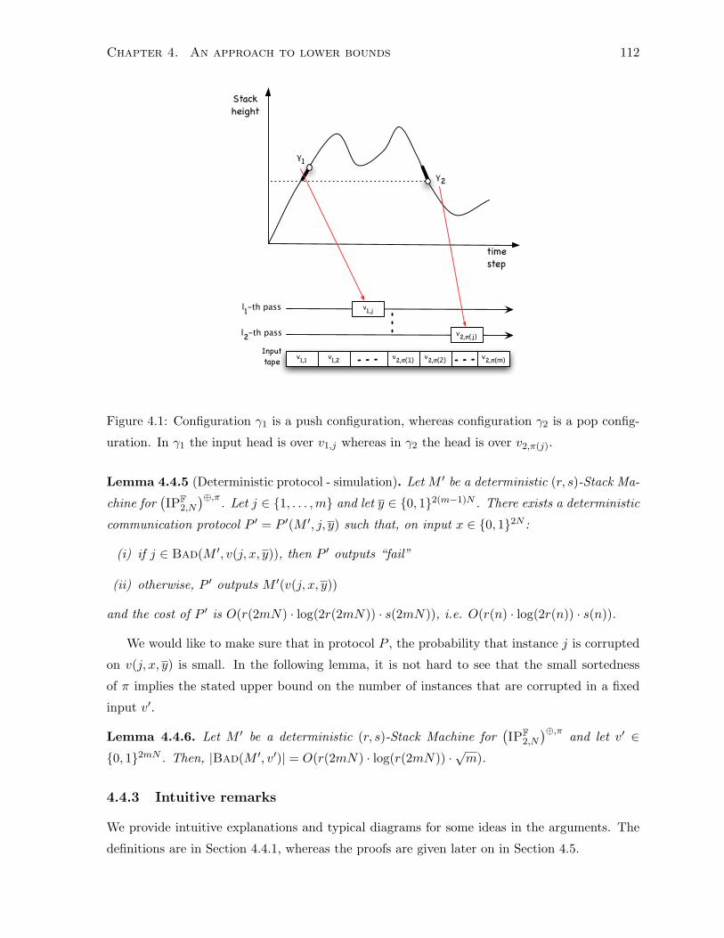
Chapter 4. An approach to lower bounds 112
Stack height
time step
Input tape
γ1
γ2
v2,π(1) v2,π(2) v2,π(m)v1,1 v1,2
l1-th pass
l2-th pass
v1,j
v2,π(j)
Figure 4.1: Configuration γ1 is a push configuration, whereas configuration γ2 is a pop config-
uration. In γ1 the input head is over v1,j whereas in γ2 the head is over v2,π(j).
Lemma 4.4.5 (Deterministic protocol - simulation). Let M ′ be a deterministic (r, s)-Stack Ma-
chine for(IPF
2,N
)⊕,π. Let j ∈ 1, . . . ,m and let y ∈ 0, 12(m−1)N . There exists a deterministic
communication protocol P ′ = P ′(M ′, j, y) such that, on input x ∈ 0, 12N :
(i) if j ∈ Bad(M ′, v(j, x, y)), then P ′ outputs “fail”
(ii) otherwise, P ′ outputs M ′(v(j, x, y))
and the cost of P ′ is O(r(2mN) · log(2r(2mN)) · s(2mN)), i.e. O(r(n) · log(2r(n)) · s(n)).
We would like to make sure that in protocol P , the probability that instance j is corrupted
on v(j, x, y) is small. In the following lemma, it is not hard to see that the small sortedness
of π implies the stated upper bound on the number of instances that are corrupted in a fixed
input v′.
Lemma 4.4.6. Let M ′ be a deterministic (r, s)-Stack Machine for(IPF
2,N
)⊕,π and let v′ ∈0, 12mN . Then, |Bad(M ′, v′)| = O(r(2mN) · log(r(2mN)) ·
√m).
4.4.3 Intuitive remarks
We provide intuitive explanations and typical diagrams for some ideas in the arguments. The
definitions are in Section 4.4.1, whereas the proofs are given later on in Section 4.5.
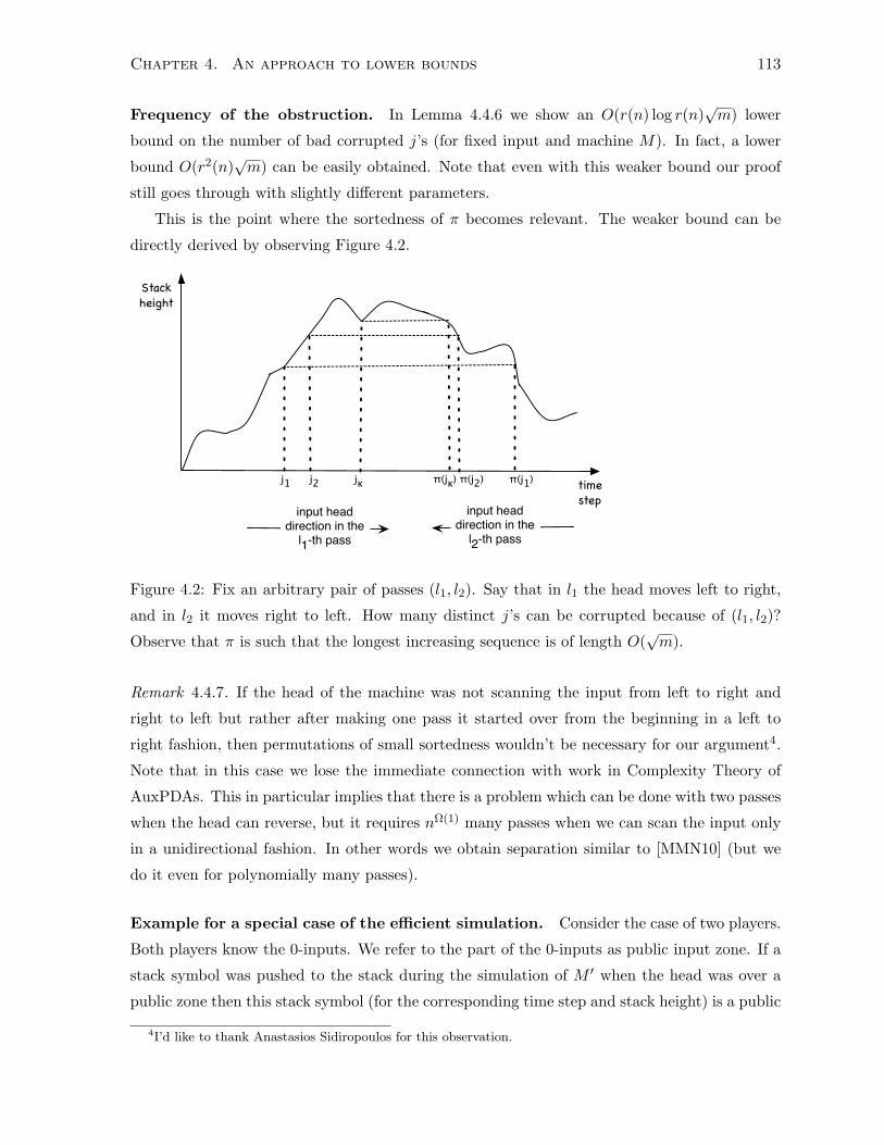
Chapter 4. An approach to lower bounds 113
Frequency of the obstruction. In Lemma 4.4.6 we show an O(r(n) log r(n)√m) lower
bound on the number of bad corrupted j’s (for fixed input and machine M). In fact, a lower
bound O(r2(n)√m) can be easily obtained. Note that even with this weaker bound our proof
still goes through with slightly different parameters.
This is the point where the sortedness of π becomes relevant. The weaker bound can be
directly derived by observing Figure 4.2.
j1 j2 jκ π(jκ) π(j2) π(j1)
input headdirection in the
l1-th pass
input headdirection in the
l2-th pass
Stack height
time step
Figure 4.2: Fix an arbitrary pair of passes (l1, l2). Say that in l1 the head moves left to right,
and in l2 it moves right to left. How many distinct j’s can be corrupted because of (l1, l2)?
Observe that π is such that the longest increasing sequence is of length O(√m).
Remark 4.4.7. If the head of the machine was not scanning the input from left to right and
right to left but rather after making one pass it started over from the beginning in a left to
right fashion, then permutations of small sortedness wouldn’t be necessary for our argument4.
Note that in this case we lose the immediate connection with work in Complexity Theory of
AuxPDAs. This in particular implies that there is a problem which can be done with two passes
when the head can reverse, but it requires nΩ(1) many passes when we can scan the input only
in a unidirectional fashion. In other words we obtain separation similar to [MMN10] (but we
do it even for polynomially many passes).
Example for a special case of the efficient simulation. Consider the case of two players.
Both players know the 0-inputs. We refer to the part of the 0-inputs as public input zone. If a
stack symbol was pushed to the stack during the simulation of M ′ when the head was over a
public zone then this stack symbol (for the corresponding time step and stack height) is a public
4I’d like to thank Anastasios Sidiropoulos for this observation.
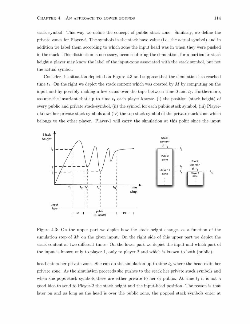
Chapter 4. An approach to lower bounds 114
stack symbol. This way we define the concept of public stack zone. Similarly, we define the
private zones for Player-i. The symbols in the stack have value (i.e. the actual symbol) and in
addition we label them according to which zone the input head was in when they were pushed
in the stack. This distinction is necessary, because during the simulation, for a particular stack
height a player may know the label of the input-zone associated with the stack symbol, but not
the actual symbol.
Consider the situation depicted on Figure 4.3 and suppose that the simulation has reached
time t1. On the right we depict the stack content which was created by M by computing on the
input and by possibly making a few scans over the tape between time 0 and t1. Furthermore,
assume the invariant that up to time t1 each player knows: (i) the position (stack height) of
every public and private stack-symbol, (ii) the symbol for each public stack symbol, (iii) Player-
i knows her private stack symbols and (iv) the top stack symbol of the private stack zone which
belongs to the other player. Player-1 will carry the simulation at this point since the input
Stack height
time step
t1 t2 t3 t4
l1
l3l4
t5
P1 public(0-inputs) P2
.
.
.
Player 1zone
Publiczone
l1
l3l4
Stack content at t1
Input tape
.
.
.
Player 1zone
l4
Stack content at t4
Figure 4.3: On the upper part we depict how the stack height changes as a function of the
simulation step of M ′ on the given input. On the right side of this upper part we depict the
stack content at two different times. On the lower part we depict the input and which part of
the input is known only to player 1, only to player 2 and which is known to both (public).
head enters her private zone. She can do the simulation up to time t2 where the head exits her
private zone. As the simulation proceeds she pushes to the stack her private stack symbols and
when she pops stack symbols these are either private to her or public. At time t2 it is not a
good idea to send to Player-2 the stack height and the input-head position. The reason is that
later on and as long as the head is over the public zone, the popped stack symbols enter at
Chapter 4. An approach to lower bounds 115
time t3 the private zone of Player-1 (and Player-2 does not know these stack symbols). Thus,
Player-1 continues to simulate after t2 and up to the lowest level l4 of the stack with the input
head over the public zone. At this point and since she knows this is the lowest level, she sends
to Player-2 the stack height, the top stack symbol, and the position of the input head. Since
this is the lowest stack height and the input head is over the publicly known zone both Players
can independently reconstruct the public stack zone from time t4 all the way to time t5, where
Player-2 takes over the simulation.
4.5 Proofs of Theorems and Lemmas
4.5.1 Proof of Theorem 4.3.1
If ε ≥ 1/4 then the statement is vacuous. Let ε < 1/4 and β := 1/4− ε. Since 0 < β < 1/4 we
have
0 <1
1− 2β<
12β
Define α such that α+ 1 is in between the two quantities above, i.e. let
α :=12( 1
1− 2β+
12β)− 1
Then, 1/(1− 2β)− 1 < α and α < 1/(2β)− 1. Hence,
β(α+ 1) < α/2
2β(α+ 1) < 1
Let m = Nα.
Assume that there exists randomized SM M that computes(IPF
2,N
)⊕,π with error δ, and
works in space s = O(nβ) and makes at most r = O(nβ) passes over the input tape. Then, by
Lemma 4.4.5 there exists a randomized communication protocol for IP2,N of cost O(r log(r)s)
and error at most δ + d(1 − δ), where d = d(N) = O(r(2mN) log(r(2mN))/√m) which for
the chosen parameters d → 0 as N → ∞. Hence, for sufficiently large inputs the error of the
protocol becomes < 1/2 and by standard arguments, repeating P a constant number of times
and taking majority vote, we get a protocol for IP2,N of cost o(N) with error at most 1/3,
which contradicts [CKS03].
4.5.2 Proof of Theorem 4.3.2
Let Mq denote the deterministic (r, s)-Stack Machine obtained by running M with random
string q.
Chapter 4. An approach to lower bounds 116
Let D be any distribution on the space 0, 12N of inputs to f = IP. Below, we give a
randomized protocol PD for f with cost and error as described in Theorem 4.3.2, but with
error computed over the choice of the input x from D and of the random coins ρ; note that
these random coins is the public randomness, and in particular q will be a substring of ρ. By
standard arguments (due to the non-uniformity of the Communication Complexity model), we
can fix ρ to obtain a deterministic protocol with the same error, but only over the choice of
x from D. Since such a protocol exists for every distribution D, by Yao’s min-max principle
(e.g., Theorem 3.20 in [KN97]), the conclusion of Theorem 4.3.2 follows.
If D has support only on 0-inputs or only on 1-inputs, PD is trivial. Otherwise, let D0 = D
conditioned on f(x) = 0.
Consider the following protocol PD:
On input x ∈ 0, 12N , where Player-i gets xi ∈ 0, 1N , and shared random string ρ:
Publicly draw j uniformly from 1, . . . ,mpublicly draw y = (y1, . . . , ym−1) from Dm−1
0
publicly draw q uniformly
Run P ′ = P ′(Mq, j, y) (from Lemma 4.4.5) on input x, simulating Mq(v(x, j, y))
If P ′ outputs “fail”, then PD outputs 1. Else, PD outputs the same value as P ′
The cost of PD is equal to the cost of P ′ which is O(r(2mN))s(2mN)). To argue about the
error in PD we define the following events:
A = A(x, ρ): PD is correct on input x with coins ρ
B = B(q, v): M is correct on input v with coins q and
C = C(j, q, v): j /∈ Bad(Mq, v).
By Lemma 4.4.5, the simulation in P ′ fails if and only if C. Let α = Prx[f(x) = 0]. We
write Pr[A] = α · Pr[A|f(x) = 0] + (1− α) · Pr[A|f(x) = 1].
For the right term, consider the conditioning f(x) = 1. Then, PD is correct if either the
simulation in P ′ fails (and PD correctly outputs 1), or the simulation in P ′ does not fail and M
is correct, thus, C ∨ (C ∧ B) ⇒ A, in particular B ⇒ A, so Pr[A|f(x) = 1] ≥ Pr[B|f(x) = 1].
The event f(x) = 1 is independent of the choice of q, and by the correctness condition of M ,
∀v,Prq[B(q, v)] ≥ (1− δ). Hence, Pr[B|f(x) = 1] = Pr[B] ≥ (1− δ).For the left term, consider the conditioning f(x) = 0. Then, PD is correct whenever
the simulation in P ′ works and M is correct, thus B ∧ C ⇒ A, and Pr[A|f(x) = 0] ≥Pr[B|f(x) = 0] Pr[C|B, f(x) = 0]. As before, Pr[B|f(x) = 0] ≥ (1 − δ). Next, j is clearly
statistically independent of x and q. Furthermore, under the conditioning f(x) = 0, we claim
that j is statistically independent from v. To see this, notice how the distribution obtained
Chapter 4. An approach to lower bounds 117
on pairs (j, v) in PD constitute the same as independently choosing m 0-inputs from D0 and
combining them in v, and choosing j uniformly from 1, . . . ,m. Thus, in the expression
Pr[C(j, q, v)|B(q, v), f(x) = 0], the conditioning depends on (x, v, q), C itself depends on j, and
j is statistically independent from (x, v, q). By Lemma 4.4.6, ∀(q, v),Prj [C(j, q, v)] ≥ (1 − d).
Then, Pr[C|B, f(x) = 0] = Pr[C] ≥ (1− d).
Putting everything together gives the claimed error bound, Pr[A] ≥ 1− (δ + d(1− δ)).
4.5.3 Proof of Lemma 4.4.6
Let i1 6= i2 ∈ 1, 2 be the identifiers for the two players as in Definition 4.4.3. We say that
instance j ∈ Bad(M ′, v′) is corrupted by the pair (l1, l2) if the latter is the lexicographically
smallest such tuple satisfying the conditions in Definition 4.4.3 for instance j. We upper bound
the number of instances corrupted by one pair.
Let J ⊆ 1, . . . ,m be the distinct instances corrupted by the same pair (l1, l2).
Claim 4.5.1. k := |J | = O(√m)
Proof. Let these instances be indexed by j1, . . . , jk such that π−1i1
(j1) < π−1i1
(j2) < · · · < π−1i1
(jk).
Assume that both l1 and l2 are odd. Then, the head of M ′ scans vi1 during pass l1 from left
to right. So, M ′ first visits vi1,π−1i1
(j1), then vi1,π−1i1
(j2), and so on, up to vi1,π−1i1
(jk). Recalling
Definition 4.1.1, if πi1 = π (recall that sortedness(π) = O(√m)) then k = O(
√m). Else,
suppose that πi1 = id and πi2 = π. For a ∈ 1, . . . , k, let γa,1, γa,2 be the configurations
mentioned in Definition 4.4.3. By this definition, the stack level cannot drop between γa,1
and γa,2, so then we must have γ1,1 ≺ γ2,1 ≺ · · · ≺ γk,1 ≺ γk,2 ≺ · · · ≺ γ2,2 ≺ γ1,2. Since
we assumed l2 is also odd, the head is also moving left to right in pass l2, so we obtain that
π−1i2
(jk) < · · · < π−1i2
(j2) < π−1i2
(j1). Therefore, k = O(√m). But either πi1 = π or πi2 = π (and
the other player has the identity permutation), where recall that sortedness(π) = O(√m). It is
easy to see that the relative parities of l1 and l2 change this argument only in that we might
obtain a monotone increasing subsequence instead of a monotone decreasing one. Thus, every
pair can corrupt at most O(√m) instances.
Next, consider A ∈ 0, 1r×r, where A[l1, l2] = 1 iff some instance is corrupted by the pair
(l1, l2). We count the number of 1s in A. Note that A is upper triangular, because for a pair
to corrupt an instance we must have l1 ≤ l2.
Moreover, for k ≥ 1, consider the diagonal l2 − l1 = k, and two entries on this diagonal
that are k′ cells apart, for 1 ≤ k′ < k. We claim that we cannot have A[l1, l1 + k] = 1 and
A[l1 + k′, l1 + k+ k′] = 1. Assume this were true. Then, some instance j is corrupted because a
symbol is pushed on the stack in scan l1 and popped in scan l1 + k, and another instance j′ is
Chapter 4. An approach to lower bounds 118
corrupted because a symbol is pushed on the stack in scan l1 +k′ and popped in scan l1 +k+k′.
But, with these settings, l1 < l1 + k′ < l1 + k < l1 + k + k′, which contradicts the way a stack
works.
Hence, for k ≥ 1, the diagonal l2 − l1 = k can contain at most r/k 1s. In total, we have
that A contains at most O(r log r) 1s. Thus, |Bad(M ′, v′)| ≤ O(r log r√m).
4.5.4 Proof of Lemma 4.4.5
Let n,m,N, s, r be as in the lemma. Let M ′ be a deterministic nonuniform SM with space
bound s and pass bound r. Let j ∈ [m] and let y be a sequence of m− 1 inputs to f .
Our goal is to show that there exists a deterministic 2-player communication protocol P ′ =
P ′(M ′, j, y) that, on input x,
1. if j ∈ Bad(M ′, v(j, x, y)), then P ′ outputs “fail”;
2. otherwise, P ′ correctly simulates M ′ and outputs M ′(v(j, x, y));
3. the cost of P ′ is O(r · log(2r) · s).
Fix an input x and let v := v(j, x, y). Observe that the players in P ′ share j and y, and
their private inputs are x1, x2. Thus, from the input v to M ′, they each know all instances
i 6= j, and from instance j, player p only knows xp. Furthermore, observe that the goal of P ′ is
not to compute f , but rather, to compute the output of M ′ on v.
Private Input Symbols. We say that an input symbol from v is private to player p if it’s
part of vp,ϕ−1p (j), which is where xp, the input to player p, is embedded in v. Input symbols
that are not private to any player are public.
Private Stack Symbols. Let Γ be the sequence of configurations of M ′ on v. Consider a
configuration γ ∈ Γ and look at the contents of the stack in γ. For every symbol ξ appearing on
the stack, we say that the stack symbol ξ is private to player p if the input head was scanning
an input symbol private to player p in the configuration prior to the transition in which ξ was
pushed on the stack. A stack symbol that is not private to any player is public.
Input- and Stack-Private Configurations. We say that configuration γ is input-private
to player p if the input head in γ is scanning an input symbol that is private to player p. We
say that configuration γ is stack-private to player p if it is not input-private to player p, the
transition out of γ is a pop transition and the top stack symbol in γ is private to player p. A
configuration that is neither input- nor stack-private is public.
Chapter 4. An approach to lower bounds 119
Intuitively, player p is responsible for simulating the transitions out of configurations that
are input- or stack-private to itself. Note that, there exists a configuration that is input-private
and stack-private to two different players if and only if j ∈ Bad(M ′, v).
Hollow View. We say that player p sees a hollow view of the stack in a configuration γ if
player p knows:
(i) the stack height;
(ii) for every symbol on the stack, whether it is public or private
(iii) all stack symbols that are public or private to itself; and
(iv) for p′ 6= p, the top stack symbol in any contiguous zone of symbols private to player p′.
We say that a player sees a hollow view of the configuration γ if it knows the state of the SM,
the location of the input head, and it also sees a hollow view of the stack in γ.
Some Simple Facts. In the protocol P ′, the players simulate Γ transition by transition,
always using hollow views of the configurations along the way. We observe the following facts.
(1) If a player p sees a hollow view of a configuration γ, then that player can determine
whether γ is public, input-private to the other player (since it knows the location of the
input head), or stack-private. There is a mild subtlety involving the latter, specifically,
the definition of γ being stack-private involves knowing that the transition out of γ is a
pop transition. To this end, observe that, by virtue of part (iv) of the hollow view of the
stack, if γ is not input-private, then player p knows the transition out of γ, even in the
case when the top stack symbol is private to player p′.
(2) If a player sees a hollow view of a public configuration γ, then that player can compute a
hollow view of the configuration following γ (denoted by next(γ)).
(3) As long as j /∈ Bad(M ′, v), if player p sees a hollow view of a configuration γ which is
input- or stack-private to player p, then player p can compute a hollow view of next(γ).
(4) If player p sees a hollow view of a configuration γ that is input-private to itself, it can
detect whether γ is stack-private to p′.
The Protocol. We now describe the protocol P ′. The sequence Γ is split into several con-
tiguous sections, each of which is of exactly one of the following three types:

Chapter 4. An approach to lower bounds 120
(a) Public sections. These sections start with some public configuration (not just any), they
consist exclusively of public configurations, and they extend up to, and including, the first
configuration which is no longer public.
Inductively, by facts (1) and (2) above, if both players have a hollow view of the configu-
ration at the beginning of a public section, they can all simulate the entire public section
starting at that configuration. At the end of the section, the control of the simulation is
given to the other player. All this is done without any communication.
(b) Input-private sections. Each such section starts with, and contains, a maximal sequence
of input-private configurations to some player p, and it ends with the single configuration
immediately following that sequence. The latter might be public, or input-private to p′,
or stack-private to any of the players.
Inductively, by facts (1), (3) and (4) above, if player p sees a hollow view of the configura-
tion at the beginning of a sequence of input-private configurations to itself, it can either
detect that instance j is corrupted, in which case player p aborts the simulation and the
protocol P ′ outputs “fail”, or simulate the entire section. Let γ′ be the configuration at
the end of the section. At this point, player p communicates:
(v) the state in γ′;
(vi) the input head position in γ′;
(vii) the stack height L′ in γ′;
(viii) the top stack symbol in γ′;
(ix) the lowest stack height L′′ achieved in a configuration between γ and γ′; and
(x) the stack symbol at level L′′.
(c) Mixed stack-private and public sections. Each such section begins with a configuration
that is stack-private to a player p, and contains a mix of configurations that are either
stack-private to p or public.
Let γ be the configuration at the beginning of such a section. Let p be the player to
which it is stack-private, and assume this player has a hollow view of γ. Let γ′ be the first
configuration following γ which is either input-private to any player, or stack-private to
p′. Inductively, by facts (1), (2) and (3) above, player p can simulate the entire sequence
of configurations between γ and γ′.
The key technical point of this entire proof is determining the right place where a player
stops a privately simulated section of type (c). It turns out that this is not γ′: doing so
could result in public symbols being placed on the stack which would only be known to
Chapter 4. An approach to lower bounds 121
player p, unless they would be subsequently communicated, which would affect the cost
of the protocol. Furthermore, it turns out it is also a bad idea for player p to end this
section at the first public configuration encountered: the subtlety here is that the stack
level might go up and down, and each time it goes down a few private stack symbols are
being popped from the same contiguous section of private stack symbols. This scenario
would hurt the cost of the protocol, for we could only bound the amount of communication
in terms of the length of the contiguous zones of private stack symbols, which can be large.
Instead, player p, looking at the entire sequence from γ to γ′, computes the minimum
possible stack level for this section, and finds the last configuration γ′′ preceding, and
possibly equal to, γ′ where the stack level is minimal. At this point, player p communicates
(v)—(viii) for configuration γ′′. Observe that, by definition of γ′′, (ix) and (x) are equal
to (vii) and (viii), respectively.
Having defined the types of simulated sections, we show that the players have enough
information to carry out the simulation. Let A be the number of different sections in the
simulation. We claim that for every 1 ≤ a ≤ A, all players eventually see a hollow view of the
configuration at the beginning of section a. We prove this by induction on a.
For a = 1, observe that the initial configuration is either public or input-private to player
1. In either case, all players see a hollow view of the stack, because the stack is empty.
Inductively, assume both players have a hollow view of the configuration γ at the beginning
of section a ≥ 1.
If the section is of type (a), by fact (2), all players see a hollow view of the configuration at
the end of this section.
If the section is of type (b), let p be the player to which γ is input-private. Clearly, by
fact (3), p itself sees a hollow view of the configuration γ′ at the end of the section. After p
communicates (v)—(x), player p′ updates its view of the stack as follows: it truncates the stack
at height L′′; fills it to the height L′ with symbols private to player p; to compute part (iv) of
the hollow view, player p′ obtains the top stack symbol in γ′ from (ix), and the stack symbol
at level L′′ from (x). Taking into account (v) and (vi), now player p′ sees a hollow view of γ′.
If the section is of type (c), let p be the player to which γ is stack-private. Let γ′′ be the
configuration where this section ends. Clearly, by facts (2) and (3), player p sees a hollow view
of γ′′. After p communicates (v)—(viii) at the end of the section, player p′ updates its view of
the stack as follows: it truncates the stack at height L′; and it updates the top stack symbol
using (vii). Taking into account (v) and (vi), now p′ sees a hollow view of γ′′.
This completes the description of the protocol P ′. If j /∈ Bad(M ′, v), the players get to
the final configuration, obtaining the output of M ′ on input v. If j ∈ Bad(M ′, v), one of the
Chapter 4. An approach to lower bounds 122
players detects this during a section of type (b), the simulation is aborted, and P ′ and outputs
“fail”.
The Cost of the Protocol. We now compute the amount of communication in P ′. The
number of sections of type (b) is 2r, one for each player, in every pass. For 1 ≤ a ≤ 2r, let Sabe the a-th section of type (b) and let γa and γ′a be the configurations at the beginning and at
the end of Sa.
Fix a < 2r, and look at the stack in γ′a. It contains public stack symbols, and several
contiguous zones of private stack symbols, at most one such zone for every previous section of
type (b). Furthermore, and crucially, observe that:
Claim 4.5.2. The number of sections of type (c) in between Sa and Sa+1 equals the number of
different contiguous zones of private stack symbols from γ′a (the end of Sa) from which a symbol
is popped before γa+1 (the beginning of Sa+1).
Proof of Claim 4.5.2. This critical property follows from the way sections of type (c) are ter-
minated. Specifically, we claim it is impossible for two different sections of type (c) between
Sa and Sa+1 to pop symbols from the same contiguous zone of stack symbols private to some
player p.
Assume this was the case for some sections S′1 and S′2. In between them, there can be no
input-private configurations (by definition of Sa and Sa+1), and also no configurations stack-
private to player p′ (otherwise, the zones of private stack symbols corresponding to S′1 and S′2
would not be contiguous). Hence, all configurations between S′1 and S′2 are either public, or
stack-private to player p. Moreover, the stack level in S′2 is strictly lower than in S′1. Then,
player p should not have ended section S′1 so early, instead, it should have simulated the entire
section of configurations between S′1 and S′2, and then it should have continued with S′2.
Clearly, for every contiguous zone of private stack symbols from which symbols are popped
in between Sa and Sa+1, there must be at least one associated section of type (c). By the
argument above, there will be exactly one such section of type (c).
Let γ2r+1 denote the final configuration. Consider the (2r)×(2r) matrix B, whereB[a1, a2] :=
1 if, in between γ′a2(the end of Sa2) and γa2+1 (the beginning of Sa2+1 or the final configuration),
a private stack symbol is popped that was pushed in Sa1 ; and B[a1, a2] := 0 otherwise.
Claim 4.5.3. There are at most O(2r · log(2r)) 1 entries in B.
Proof of Claim 4.5.3. The matrix is 0 under the main diagonal, because for a symbol from Sa1
to be popped after Sa2 , we must have a1 ≤ a2. Consider the diagonal a2 − a1 = j for some
j ≥ 1. We claim that it is impossible to have B[a, a + j] = 1 and B[a + j′, a + j + j′] = 1
Chapter 4. An approach to lower bounds 123
for some a and some 0 < j′ ≤ j. Assume B[a, a + j] = 1, so in between γ′a+j and γa+j+1 a
symbol is popped that was pushed in Sa. But then, the stack in γa+j+1 can no longer contain
any symbols pushed in Sa′ , for any a′ such that a < a′ ≤ a + j. In particular, for a′ = a + j′,
all symbols pushed in Sa+j′ are no longer on the stack in γa+j+1, which precedes, or equals,
γa+j+j′ , Hence, it is impossible to have B[a+ j′, a+ j + j′] = 1.
The argument above shows that the matrix B contains at most 2r/(j + 1) 1 entries on the
diagonal a2 − a1 = j. Hence, in total, it contains at most O(2r log(2r)) 1 entries.
Lastly, we observe the following.
Claim 4.5.4. The number of sections of type (c) in between Sa and Sa+1 is at most the number
of 1 entries in column a of matrix B.
Proof of Claim 4.5.4. By Claim 4.5.2, every section of type (c) in between Sa and Sa+1 is
associated with a contiguous zone of stack symbols from γ′a (the end of Sa) that are private to
some player p. Since all private stack symbols pushed in Sa′ are contiguous on the stack (this
is true at any point of the simulation), we see that there can be at most one section of type
(c) for every section Sa′ such that symbols from Sa′ are popped in between Sa and Sa+1, or,
equivalently, such that B[a′, a] = 1.
Putting everything together, first observe that sections of type (a) do not result in any
communication. There are 2r sections of type (b), and by Claims 4.5.3 and 4.5.4, there are a
total of O(2r · log(2r) sections of type (c).
And the end of every section of type (b) or (c), items (v)—(x) are communicated. The full
state takes O(s) bits, the input head position takes logN ≤ O(s) bits, the stack height takes
O(s) bits by Fact 3.1.3. Thus, every communication consists of O(s) bits. The total cost of the
protocol P ′ is thus O(2r log(2r) · s).
Chapter 5
Some Remarks on Cryptography in
Streaming Models
We initiate the study of Streaming Models for Private-Key Cryptography from generic crypto-
graphic assumptions. This is the last, smallest, and technically simplest part of the thesis. The
main technical contribution regards lower bounds. We also observe that it is possible to have
logspace streaming Cryptography by directly applying, in a non-black-box way1, the main con-
struction of Applebaum, Ishai and Kushilevitz [AIK06a] on Cryptography in NC0. The lower
bounds we have obtained indicate that the connection with Cryptography in NC0 is in some
sense necessary.
In Section 5.1 we provide a preliminary motivating discussion which also improves the
main result of [KGY89]. Basic definitions, notation, preliminary results and the non-black-box
construction are given in Section 5.2. Note that there are certain changes with respect to the
conventions made in the previous chapters. Section 5.3 investigates the possibility of basing
the streaming computation of OWFs on known assumptions about OWFs, e.g. the hardness
of Factoring or Subset-Sum, or on other generic assumptions. We answer these questions
(unconditionally) in the negative by using standard tools from Communication Complexity,
ideas from crossing sequence arguments, and elementary Information Theory techniques. In
Section 5.4 we briefly discuss at an intuitive level the relation between graph-theoretic properties
and cryptographic hardness. In Section 5.5 we provide slight improvements on the streaming
computation of the OWF, and conjectures regarding logspace streaming cryptography. These
conjectures shape the main theoretical motivation for studying Cryptography in Streaming
models. 2 Finally, Section 5.6 concludes with our view on the future of Streaming Models for
1As usual, non-black-box means that the construction makes use of the “code” for computing the primitive.2Also, in [Pap10] we have used the logspace streaming computation of the OWF to show under generic
cryptographic assumptions that there is ε > 0 such that SATpw[logε n] ∈ PolyLogSpace ∩ NP and SATpw[logε n] /∈
124
Chapter 5. Some Remarks on Cryptography in Streaming Models 125
Cryptography.
5.1 Motivating discussion
Assumption 1 (p. 17), regarding the existence of 2nε-hard OWFs, is the main assumption on
which our constructions rely.
Example 5.1.1. We motivate the discussion by using this generic assumption to construct
a OWF in a streaming manner. Let f be as in Assumption 1 computable in time and in
particular in space nk, for some constant k. Let s(n) = logk′n for some k′ > k/ε. Consider
an O(s(n))-bounded transducer which makes a single pass over the input and works as follows.
Read the first s′(n) := s(n)1/k bits and copy them on the work-tape. Let this part of the
input be α ∈ 0, 1s′(n). Now, compute and output f(α). By the choice of k′ we have that
2s′(n)ε > p(n) for every polynomial function p(n), and thus we obtain the following fact.
Fact 5.1.2. If Assumption 1 holds, then there exists a OWF computable by a space bounded
Turing Machine with a single pass over the input seed, for sufficiently large ω(log n) space.
In this example, it is crucial that s′(n) is super-logarithmic. By strengthening Assumption
1 to hold for every ε < 1 and requiring f to be computable in linear space, we construct a OWF
for every s(n) = log1+ε′ n. But, when the workspace of the machine becomes O(log n) a similar
construction is no longer secure.
The above example can be extended to construct a PRG, if the OWF in Assumption 1 is
a OWP. For this we apply the Goldreich-Levin construction (see Section 1.1.2) by partitioning
α = (x, r) to output: x, f(r), 〈x, r〉, and we append to the output the remaining (i.e. excluding
α) part of the seed.
Remark 5.1.3. Note that generalizing the above construction using (1.1.1), we can compute in
polylogarithmic space a PRG of polynomial length. One question is whether the 2nε
hardness
in the OWP is necessary for the construction of the PRG. The black-box separation in Section
2.3 implies that for natural variants of the above construction, we cannot get around the 2nε
hardness.
The following lemma improves on the main result3 of [KGY89] and indicates the concep-
tual difficulty in constructing O(log n)-streaming OWFs. Allender in his PhD thesis4 [All85]
obtained an even stronger result, which states that functions computable in the same way as
in Lemma 5.1.4, are in fact invertible in NC.
BPP.3[KGY89] shows that no PRG of linear stretch can be computed in logspace and a constant number of passes.
Lemma 5.1.4 implies that no 0, 1n → 0, 1n+1 PRG exists, since a PRG is in particular a OWF.4I’d like to thank Eric Allender for bringing this result to my attention.
Chapter 5. Some Remarks on Cryptography in Streaming Models 126
Lemma 5.1.4. Let k ∈ Z+ be a constant, and f be a function computed by a logspace transducer
that makes k passes over the input. Then, there exists an algorithm that given f(x) computes
x′ ∈ f−1(f(x)) in time polynomial in |x|.In particular, there does not exist a OWF computable in logspace with a constant number of
passes over the input.
Proof. We rely on Corollary 3.5.11 which states that NL[O(1)] = NL. For given y = f(x)
consider the Turing Machine M that computes f and construct non-deterministic M ′ which
guesses x and makes at most a constant number of passes over the non-deterministic tape and
compares the outputted bits with y. Simulate, M ′ in polynomial time and output the certificate
x for an accepting branch of the computation tree.
5.2 Definitions and the logspace streaming computable OWF
5.2.1 Definitions and conventions
In this chapter we adopt, modulo a few modifications (see below), the definitions and nota-
tion of Section 3.1. For definitions of width parameters see Section 3.5.2. For definitions of
Communication Complexity problems and results from previous work see Section 4.1.
For the space bound s(n) of Turing Machines, we have s(n) = Ω(log n). We parametrize
on the number of passes over the input. Following the conventions in [AIK06a], we abuse
notation and we write NC0 to refer to the functional analog of NC0, where the cir-
cuits are assumed to be polytime uniform5. All space-bounded TMs have an additional
read-only, polynomially long advice tape which contains a P-uniform advice, unless mentioned
otherwise. An s(n) space bounded transducer, is a Turing Machine with a P-uniform advice
tape, a read-only input tape, working memory of total size s(n), and a write-only output
tape. We abuse standard notation and we write L/poly to denote the class of functions com-
putable by logspace transducers with a P-uniform advice. We define the class of functions
PASSES-SPACE(r(n), s(n)) to be the class of functions computable by O(s(n)) space bounded
transducers that make at most r(n) passes (i.e r(n)− 1 head-reversals) over the input.
The term s(n)-streaming computation refers to an s(n)-space transducer which makes logO(1) n
passes over the input. In general, streaming computation refers to O(log n)-streaming compu-
tation.
Let f ∈ NC0 and let C := Cn be a family of NC0 circuits computing f . We define the
family of dependency graphs Gn of C as follows. The dependency graph Gn = ((I,O), E) for
5It is possible to weaken the form of uniformity to logspace uniform by additional assumptions for latticeproblems.
Chapter 5. Some Remarks on Cryptography in Streaming Models 127
Cn is a bipartite graph where I and O are the two sides of bipartization such that I,O are the
set of input and output gates of Gn respectively. There exists an edge between u ∈ I and v ∈ Oif there is a dipath of wires in Cn with endpoints u and v. If the circuit family is clear from
the context then we write “dependency graphs of f” to refer to the dependency graphs of the
particular circuits6.
In the proof of Lemma 5.3.4 (see below) we make use of bipartite expanders. A bipartite
(n, d, ε) expander is a graph G = ((L,R), E), where |L| = |R| = n, it has a maximum degree
d, and the following holds: for all X ⊆ L where |X| ≤ n/2, then Γ(X) ≥ (1 + ε)|X|, where
Γ(X) denotes the neighborhood of X. For an excellent overview, existence, and constructions
of expanders see [HLW06].
5.2.2 Permuted inputs and outputs
The following simple observation is essential for the efficient streaming computation of OWFs.
Consider permutations acting on strings as follows.
Definition 5.2.1. Let x := x1 . . . xn ∈ 0, 1n and π ∈ Sym(n), where Sym(n) is the group of
permutations on 1, . . . , n. Then, π(x) denotes the string xπ(1) . . . xπ(n). A family of permu-
tations πn is t(n)-time index-computable if given n and j the value πn(j) is computable in
time O(t(n)).
The security of OWFs is invariant under permutations acting on domain or image elements.
Fact 5.2.2. Let f : 0, 1∗ → 0, 1∗ be a OWF. Then, for every x and polytime index-
computable π on |x| letters, and τ on |f(x)| letters, the functions f(π(x)), τ(f(x)) and τ(f(π(x)))
are also OWFs.
Similarly to OWFs the above fact holds for PRGs.
5.2.3 A OWF in PASSES-SPACE(logO(1) n, log n)
The next Section 5.3 indicates the conceptual difficulty of constructing a OWF in logarithmic
space. Indeed, we believe that the straightforward construction we present in this section,
wouldn’t be possible without (e.g. reproving parts of) the work for Cryptography in NC0.
We will just be using the statement of the theorem from [AIK06a] - see [AIK08] and also
[AIK06b, AIK06a, AIK07] for the quite interesting details.
In [AIK06a] the authors show how to compile any function f computable in polynomial
time as a function f ′ ∈ NC0, where f ′ in some sense preserves security properties of f . For this
6One could have similarly defined the dependency graph of the function f , but in this work the relevantconcepts are about families of circuits under certain transformations.
Chapter 5. Some Remarks on Cryptography in Streaming Models 128
compilation they need one more assumption, namely that there exists an Easy-PRG, i.e. a PRG
computable7 in ⊕L/poly that stretches n bits to n+ 1. In other words, a polytime computable
function can be compiled as a function in NC0 preserving security properties, given that a
PRG in ⊕L/poly exists. Using the recent work of Haitner, Reingold, and Vadhan [HRV10] this
assumption can be weakened to an Easy-OWF.
Assumption 3. There exists an Easy-OWF (OWF), which is a OWF computable in ⊕L/poly.
Therefore, a corollary of [AIK06a, HRV10] is the following theorem. Given a very hard OWF
f there is ε > 0 such that F (xx′) = f ′(x)00 . . . 0 is one-way, where f ′ is the NC0 analog of f and
|x| = logε n, n = |xx′|. Then, we compute in logspace and poly-log many passes by computing
each (among the poly-log many) output bits of f ′(x). This construction is straightforward but
still non-black-box - we really need the description of the NC0 circuit that computes the OWF
to do the logspace computation.
Theorem 5.2.3. Suppose that Assumption 1 and Assumption 3 hold true; i.e. a 2nε
- hard
OWF and an EOWF exist. Then, there exists ε′ > 0 and a OWF F ∈ PASSES-SPACE(logε′n, log n).
Given the discussion in Example 5.1.1 it seems counter intuitive why such a construction
is at all possible. This is achieved using the machinery of Cryptography in NC0. Some im-
provements are also possible - see Section 5.5. Moreover, the lemmas in Section 5.5 relate to
our main conjectures relating Cryptography in Streaming Models with fundamental questions
in Cryptography.
5.3 Obstacles to Streaming Cryptography - On the necessity of
Cryptography in NC0
Recall the construction of Example 5.1.1, and the lower bound of Lemma 5.1.4. Intuitively,
starting from an arbitrary very hard OWF π it seems impossible to reduce the working space
of the machine to O(log n) and still be able to securely compute a OWF π′ without making too
many passes over the input seed. In this section we discuss in greater detail why we cannot base
Streaming Cryptography on standard and other plausible assumptions, without making addi-
tional assumptions regarding cryptographic hardness, or the existence of cryptographic functions
with special properties of their computation. In other words, we provide conceptual evidence
that goes against Theorem 5.2.3.
We show (i) that computing instances for Factoring and Subset-Sum by adding and
multiplying numbers requires simultaneously polynomial space and passes over the input seed,
7Recall that P-uniform ⊕L is the class of languages characterized by non-deterministic logspace machineswhich accept iff the number of accepting paths is odd. The functional ⊕L/poly is defined similar to L/poly.
Chapter 5. Some Remarks on Cryptography in Streaming Models 129
(ii) in general, there is no simulation between NC0-circuits (as always our circuits have multiple
outputs) and logspace transducers with polynomially many passes over the input, and (iii) in
general, there is no simulation of a O(log1+ε n)-streaming computation by a O(log n)-space
bounded TM that makes nε′
many passes over the input, for some ε′ > 0.
5.3.1 Impossibility of constructions based on Factoring or Subset-Sum
We show that computing the addition and the multiplication of two numbers requires simulta-
neously polynomial number of passes and polylogarithmic space. Let Add,Mult denote the
respective computational problems.
Recall, Lemma 4.2.1 which states that an s(n)-space bounded TM for IP2,n or SetInt2,n
requires Ω( ns(n)) passes. Instead of obtaining the lower bound for Mult and Add by modifying
the reduction in the proof of Lemma 4.2.1, we provide a unified treatment.
Definition 5.3.1. Let f, g : 0, 1∗ → 0, 1∗. We write f ≤c,l g, f reduces to g via a
(c(n), l(n)) passes-preserving logspace reduction, where l is injective, if there exist logspace
transducers M,M ′, such that for every string x, |M(x)| = l(|x|), M makes at most c(|x|)passes, and f(x) = M ′
(g(M(x))
), where M ′ makes a single pass over its input.
Typically, we are interested in passes-preserving reductions where c(n) is a small constant
(usually one or two). The above definition can be generalized by adding as parameter the
number of passes of M ′ (not necessary generality for our results). The following is immediate
by definition.
Fact 5.3.2. Suppose that f 6∈ PASSES-SPACE(r(n), s(n)), s(n) = Ω(log n), such that f ≤c,l g.
Then, g cannot be computed with l−1( r(n)c(n) ) passes in space s(n).
Lemma 5.3.3. Mult cannot be computed in o(√
ns(n)) reversals in space s(n), and Add cannot
be computed in o( ns(n)) reversals in space s(n).
Proof. It suffices to show that IP ≤2,n2 Mult, and that SetInt ≤1,2n Add.
IP ≤2,n2 Mult: Let α = (a1, . . . , an), β = (b1, . . . , bn) ∈ 0, 1n be an instance of IP. Then, in
two passes we construct (in logspace) the input
α′ = (a1, 0, 0, . . . , 0︸ ︷︷ ︸ntimes
, a2, . . . , an−1, 0, 0, . . . , 0︸ ︷︷ ︸ntimes
, an), β′ = (bn, 0, 0, . . . , 0︸ ︷︷ ︸ntimes
, bn−1, . . . , b2, 0, 0, . . . , 0︸ ︷︷ ︸ntimes
, b1)
where α′, β′ are the binary representations of two integers. In the integer multiplication of α′β′
the 2n-th bit corresponds to the first, least significant, bit of the sum a1b1 + . . . anbn, which
coincides with the valuation of this sum over GF(2).
Chapter 5. Some Remarks on Cryptography in Streaming Models 130
SetInt ≤1,2n Add: Let x = (x1, x2, . . . , xn), y = (y1, y2, . . . , yn) ∈ 0, 1, be the charac-
teristic vectors of two sets over a universe of n elements. In a single pass construct x′ =
(x1, 0, x2, 0, . . . , 0, xn), y′ = (y1, 0, y2, 0, . . . , 0, yn). The intercalate zeros are carry-detectors. By
adding x+ y there exists a carry-detector equal to 1 iff supp(x) ∩ supp(y) 6= ∅.
In particular, this implies that Mult,Add 6∈ PASSES-SPACE(nε, logO(1) n), for some ε > 0.
Permuted inputs. It becomes more involved, and we omit presenting, lower bounds for
computing instances for Factoring and Subset-Sum when the inputs are permuted. Although
for Mult a lower bound for permuted inputs can be obtained, the same is not true for Add.
We have to consider the actual instance to Subset-Sum, which consists of nΩ(1)-many n-bit
numbers, together with the characteristic vector of the set of numbers to be added.
5.3.2 Incomparability of NC0 and PASSES-SPACE(nΩ(1), log n)
Recall that the decisional NC0 ( Decision-PASSES-SPACE(O(1),O(1)) =: REGULAR. We show
that the functional NC0 and PASSES-SPACE(nε, log n) are incomparable in some strong sense,
for some constant ε > 0.
Lemma 5.3.4. (i) PASSES-SPACE(1, 1)− NC0 6= ∅, (ii) NC0 − PASSES-SPACE(nε, log n) 6= ∅,for some constant ε > 0. Furthermore, (ii) holds in the stronger form for some fn ∈ NC0 and
gn 6∈ PASSES-SPACE(nε, log n), where gn is fn under an arbitrary permutation of its input
and output bits, for some constant ε > 0.
Proof. (i) Consider the OR function (i.e. with one output bit) of all bits. Clearly, this can be
decided by a finite state automaton. However, the output depends on all input bits and thus it
cannot be in NC0.
(ii) Consider a family of expander graphs. Here is a property of this family.
Claim 5.3.5. Fix a family of (n, 3, ε)-bipartite expanders
((Ln, Rn), E)n
. Fix a permutation
on Ln such that the permuted Ln is the sequence L = 〈a1, a2, . . . , a|Ln|〉. For two vertices
u, v ∈ L we say that they are peers if there exists w ∈ Rn connected to both. Then, there exist
two sequences A,B subsequences of L, each of length nε′
for some constant ε′ > 0, such that for
every u ∈ A there exists exactly one peer vertex in B and vice versa (in particular, |A| = |B|),
and the index (i.e. the subscript wrt the ordering) of every vertex in A is smaller than the index
of a vertex in B.
Proof sketch. Immediate by the expansion property. Consider a (contiguous) subsequence of
polynomial size then consider its neighborhood and then the neighborhood of this neighborhood.
Chapter 5. Some Remarks on Cryptography in Streaming Models 131
Let us give a few more details without getting into detailed calculations. Fix a constant α < 1
and consider a contiguous sequence S of length nα (say in the middle) of L. Let ΓR := Γ(S)
and ΓL := Γ(ΓR). Then, we know that in particular S ⊆ Γ2 and furthermore D := Γ2−S such
that |D| = Ω(nα) (this is guaranteed by expansion). Now, there are two cases to consider. One
where the vertices in D are “balanced” to the left and to the right of S, and the complementary
where no significant fraction of D is on both sides. In the first case we consider the elements
of D in the left and in the right of S to form the subsequences A and B respectively. In the
other case, we construct A with vertices from the leftmost half of S, and we construct B with
vertices from the rightmost half of D.
Define the following function f : 0, 1n → 0, 1n. Given n, consider a graph G from
a family of bipartite expander graphs as in Claim 5.3.5. G is the dependency graph of the
function f with output bits the XOR of the corresponding input bits.
Suppose that (ii) is false, i.e. gn ∈ PASSES-SPACE(nε, log n) for every ε > 0. Fix, ε < ε′,
where ε′ as in Claim 5.3.5. We show that we can decide equality (EqualN ) in the 2-party
model Communication Complexity model by communicating less than N − 1 bits, for infinitely
many string lengths N ∈ Z+.
Let N = nε′. Consider inputs where every bit other than the ones in A∪B is equal to zero.
Here is a protocol for EqualN . Player-1 is given the input corresponding to the bits of A and
Player-2 is given the bits corresponding to B. Let M be an s(n)-space bounded machine that
computes f with r(n) passes. Player-1 carries the simulation up to the point that the input
head of M enters B. At that point player-1 sends the O(log n)-bits-long configuration of M to
Player-2. Player-2 caries on the simulation of M up to the point where the head enters again
A where she sends the configuration of M to Player-1. If M outputs a bit different than 0 then
the corresponding player sends a special message (e.g. reserve the first bit as a flag for this in
every message the two players exchange) indicating that the two strings are not equal. Hence,
in total there are O(nε log n) bits communicated, which is smaller that nε′
= N .
5.3.3 Impossibility of simulating an ω(log n)-model by an O(log n)-model
We show that there is no general simulation of a (logk n)-space transducer by a transducer of
smaller memory at an expense a small number of passes over the input. Thus, we cannot base
in an obvious way the existence of OWFs on the construction of logO(1) n-streaming OWFs
given in Example 5.1.1.
Remark 5.3.6. The application of Communication Complexity we have in mind results in only
polylogarithmic (and not polynomial) bounds in the number of passes. One explanation for
this is that the ratio of the space of the two models we compare is quite small. We do not
Chapter 5. Some Remarks on Cryptography in Streaming Models 132
know how to apply a Communication Complexity reduction in this case. It seems that a new
Communication Complexity Theory with Auxiliary Inputs should be developed towards this
purpose. Technically, we proceed from elementary Information Theory principles by construct-
ing an impossible compress-decompress scheme.
Lemma 5.3.7. Let 0 ≤ ε′ < ε. There exists ε > 0 and f ∈ PASSES-SPACE(1, log1+ε n) such
that f 6∈ PASSES-SPACE(nε, log1+ε′ n).
Proof. Consider the following family of functions fn : 0, 1n → 0, 1n/2. Let N = n2 log1+ε n
and
f defined as follows f : α1, β1, . . . , αN , βN 7→ α1⊕β1, . . . , αN ⊕βN , where |αi| = |βi| = log1+ε n.
The TM with memory O(log1+ε n) in a single pass reads the corresponding αi and stores it on
its worktape and when the head moves to the first bit of βi it starts outputting the bitwise
XOR, αi ⊕ βi.Let M be a O(log1+ε′ n)-space bounded TM which computes fn. Consider the time interval
where M starts outputting the first bit of αi ⊕ βi up to the point that outputs the last bit of
αi ⊕ βi. We show that in this interval M makes at least two passes (it reverses its head at
least once). Since this happens for every pair (αi, βi) we have an Ω(N) = nΩ(1) bound on the
number of passes during the computation of M .
Suppose that we choose the input α1, β1, . . . , αN , βN uniformly at random. Let Ei be the
event that the machine makes at least two passes (one reversal) when outputting αi ⊕ βi.
Claim 5.3.8. Pr[Ei] ≤ 1N2
This claim implies that Pr[E1 ∧ . . . ∧ EN ] = 1− Pr[E1 ∨ . . . ∨ EN ] ≥ 1− 1N > 0, i.e. there is
an input where M makes Ω(N) passes.
Proof of Claim. Suppose that Pr[Ei] > 1N2 .
Since Pr[Ei] > 1N2 this means that for at least 2n/N2 > 2n−2 logn of the input strings, M
makes a single pass when outputting γi := αi ⊕ βi. Let this set of strings be Si. Note that we
need to send at least n− 2 log n bits to describe an arbitrary element of Si. In what follows, we
show how to construct an impossible compress-decompress scheme.
Consider two players communicating over a noiseless channel, where Player-I is given a
message from Si and he sends it to Player-II. We show that Player I sends K ′ = n−Ω(log1+ε n)
bits to communicate the message (which requires K = n−2 log n bits), which is a contradiction.
Suppose that Player-I is given x ∈ Si. He simulates M on input x. Since the input-head of
M does not change direction during the outputting of γi, wlog assume that it scans the input
tape from left to right. We consider two cases: (i) at least half of the bits of γi are output
before the input-head enters βi or (ii) otherwise, more than half of the bits are output after the
head enters βi.
Chapter 5. Some Remarks on Cryptography in Streaming Models 133
Case (i): Player-1 sends to Player-2 a message containing (1) one bit distinguishing between
Case (i) and (ii), (2) the configuration of M when the first bit of αi ⊕ βi is outputted, (3) αi,
(4) the second half of βi, (5) every bit of x except αi, βi. In total, he sends
1 +O(log1+ε′ n) + log1+ε n+log1+ε n
2+ n− 2 log1+ε n = n− Ω(log1+ε n)
many bits to Player-2. Then, Player-2 simulates M and she retrieves the first 12 log1+ε n bits of
βi, and thus she has a full description of the message with K ′ < K bits.
Case (ii): Similarly to Case (i) but now instead we transmit without actually sending the
second half of αi.
5.4 Some remarks on the relation of cryptographic hardness
and graph-theoretic properties of NC0 circuits
The work of Cryptography in NC0 brings the combinatorics of computing cryptographic primi-
tives to the level of constant depth and bounded fan-in circuits. It is plausible to assume that a
necessary condition for the dependency graph of the circuits is that it is complicated enough in
order to preserve cryptographic hardness (security of the primitive). This is implicit in works
in the area, but also explicitly stated in [AIK08, Gol00], where “graph-theoretic complexity8
is associated with expansion”. This kind of intuition works against possible constructions of
streaming models for Cryptography. Some evidence about this is given in the proof of Lemma
5.3.4. In fact, the simple non-black-box construction is based on the fact that the dependency
graph of the cryptographic function is (at a large scale) graph-theoretically very simple. In
this section we give some intuition as to why “cryptographic hardness in NC0” cannot be as-
sociated in some obvious way with “graph-theoretic complexity”. For the rest of this section
“graph-theoretically complex” means high expansion, and graphs are “simplified” by removing
edges.
Example 5.4.1. Let f be a OWF computed by NC0 circuits, and let C be such a circuit with
input of length nε, ε > 0. Consider an input x = x′x′′, where |x′| = nε and |x′′| = n− nε, and
define g(x) = g(x′x′′) = f(x′)x′′. Then, it easily follows that g is also a OWF. If f has good
expansion, g does not inherit this property. Note that g has embedded into it a polynomially
large expander graph.
8In [AIK08] this is restricted to small O(logn) “parts” of the circuits.
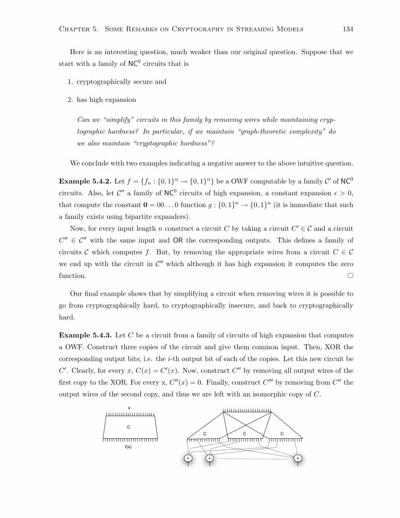
Chapter 5. Some Remarks on Cryptography in Streaming Models 134
Here is an interesting question, much weaker than our original question. Suppose that we
start with a family of NC0 circuits that is
1. cryptographically secure and
2. has high expansion
Can we “simplify” circuits in this family by removing wires while maintaining cryp-
tographic hardness? In particular, if we maintain “graph-theoretic complexity” do
we also maintain “cryptographic hardness”?
We conclude with two examples indicating a negative answer to the above intuitive question.
Example 5.4.2. Let f = fn : 0, 1n → 0, 1n be a OWF computable by a family C′ of NC0
circuits. Also, let C′′ a family of NC0 circuits of high expansion, a constant expansion ε > 0,
that compute the constant 0 = 00 . . . 0 function g : 0, 1n → 0, 1n (it is immediate that such
a family exists using bipartite expanders).
Now, for every input length n construct a circuit C by taking a circuit C ′ ∈ C and a circuit
C ′′ ∈ C′′ with the same input and OR the corresponding outputs. This defines a family of
circuits C which computes f . But, by removing the appropriate wires from a circuit C ∈ Cwe end up with the circuit in C′′ which although it has high expansion it computes the zero
function.
Our final example shows that by simplifying a circuit when removing wires it is possible to
go from cryptographically hard, to cryptographically insecure, and back to cryptographically
hard.
Example 5.4.3. Let C be a circuit from a family of circuits of high expansion that computes
a OWF. Construct three copies of the circuit and give them common input. Then, XOR the
corresponding output bits; i.e. the i-th output bit of each of the copies. Let this new circuit be
C ′. Clearly, for every x, C(x) = C ′(x). Now, construct C ′′ by removing all output wires of the
first copy to the XOR. For every x, C ′′(x) = 0. Finally, construct C ′′′ by removing from C ′′ the
output wires of the second copy, and thus we are left with an isomorphic copy of C.
+ + +
CC C C
x
f(x)
Chapter 5. Some Remarks on Cryptography in Streaming Models 135
In-depth investigation of conditions where cryptographic hardness is related to graph-
theoretic properties is a very fundamental issue. A first step has been taken in [AIK08].
5.5 Improvements on the logspace streaming computation of
the OWF and some conjectures
The naive way of using the NC0 circuit in order to compute the OWF already achieves poly-
logarithmic passes and logarithmic space. Recall, that our unconditional lower bound (Lemma
5.1.4) shows impossibility for a constant number of passes. In fact, depending on the parameter
ε in the hardness of the OWF we start with, the number of passes can be reduced to logε′n,
for ε′ > 0 arbitrarily close to 0. To that end we are going to use the Lemma 5.5.2. Note that
this lemma is expressed in a slightly more general setting than what we actually need. On the
other hand this generality is exactly what we need for stating our most interesting conjectures.
Remark 5.5.1. Lemma 5.3.4 states that we cannot compute an arbitrary NC0 function in
logspace in a streaming manner. This holds even when we allow permutations of its output
bits. Let us restrict our attention to functions computable with circuits of small pathwidth.
In this case still, in general it is not possible to compute in a streaming manner the same NC0
function of small pathwidth. This is due to trivial reasons that have to do with the ordering of
the inputs and the fact that a transducer outputs bits in order. However, in the sense of Fact
5.2.2 we have that the streaming model is robust for doing Cryptography.
Lemma 5.5.2. Let f ∈ NC0 be computable by the family F = Cn of NC0 circuits whose depen-
dency graphs have given path decompositions of width w(n). Then, for every input length n there
exist logspace index-computable permutations π, τ such that π(f(τ(x))
)∈ PASSES-SPACE(O(w(n)
logn ), log n).
Proof. The algorithm that computes π(f(τ(x))
)is a little more complicated than the algorithm
that appears in the proof of Lemma 3.5.15 henceforth denoted by A. We proceed by using A.
Note that the permutations π and τ are induced by the given path-decomposition.
Since C ∈ F is an NC0 circuit every output gate u has value a boolean function ψ of a
constant number of input variables x1, . . . , xk, where k depends on the (constant) depth of C.
Hence. ψ(x1, . . . , xk) can be expressed as a constant size k-CNF; we abuse notation and we
write ψ for this formula.
We perform some syntactic maneuvers before using A. Associate with C a k-CNF formula
φ which is the conjunction of these constant-size subformulas ψ. We are not interested in the
satisfiability of φ; we are just interested in the satisfiability of its subformulas ψ (these are the
output bits of the function).
Chapter 5. Some Remarks on Cryptography in Streaming Models 136
Observe that the given path decomposition for the dependency graph of C yields in logspace
a decomposition for the incidence graph for φ of width O(w(n)). Finally, applying the logspace
transformation [GP08] from the path decomposition of width α(n) to an ordered formula of
diameter O(α(n)), we obtain an ordered formula Φ of diameter O(w(n)). Two remarks are
in order. First Φ admits different models (it has more variables) than φ. However, all newly
introduced variables appear also as rewritings (x ↔ x′) of the initial variables. Hence, in
logspace we can consistently determine the values of the new variables in Φ. The second
remark is that the transformation in [GP08] is local in the sense that the satisfiability of the
transformed subformulas ψ is maintained.
Now, we are ready to apply A on Φ. The difference is that the role of the non-deterministic
tape is being taken by the input x to the circuit C. In the execution of A we do not care
about the satisfiability of Φ but rather the satisfiability of the (transformed) subformulas ψ. If
the subformula is satisfied during the evaluation then we output 1, whereas if it is falsified we
output 0.
Now, we are ready to state our conjecture.
Conjecture 1. There exists a 2nε-hard OWF, ε > 0 ⇐⇒ there exists an NC0 computable
OWF function of pathwidth logε′n, for some ε′ > 0.
To the best of our knowledge there is no non-trivial characterization of 2nε-hard OWFs.
None of the directions for this conjecture is trivial. To establish the ⇒ direction, by applying
[AIK06a, HRV10] it remains to derive an EOWF from a 2nε-hard OWF. For the other direction
we do not have an idea of how to proceed, but we believe that pathwidth (or treewidth) is the
most general restriction on the circuits such that the current state of knowledge could establish
such a result.
Finally, we also conjecture the following.
Conjecture 2. There exists an NC0 computable OWF function of pathwidth logε′n, for some
ε′ > 0 ⇐⇒ there exists a logspace streaming computable OWF.
For this conjecture Lemma 5.5.2 seems to be even more helpful.
All told, we believe that the following can be shown:
there is a 2nε-hard OWF ⇐⇒ there is small pathwidth OWF in NC0 ⇐⇒ there
is logspace streaming computable OWF
5.5.1 Inverting NC0 functions of small pathwidth
By construction, the OWF in Theorem 5.2.3 can be inverted in time nlogO(1) n. In fact, every
NC0 function of such pathwidth can be inverted within this time.
Chapter 5. Some Remarks on Cryptography in Streaming Models 137
[GP08] gives an algorithm that works in NSPACE(w(n)) for deciding the satisfiability of a
k-CNF formula of pathwidth w(n). Since the i-th output gate ui of an NC0 circuit is naturally
associated with a k-CNF ψi of input bits, if the given value of the output is yi, then the formula
ψ ↔ yi is satisfied for values of input bits that evaluate to the correct y. Observe that if the
circuit has a path decomposition of width w(n) then we can write a k-CNF formula φ satisfiable
for an x ∈ 0, 1n such that f(x) = y, and φ has a logspace computable path decomposition of
width O(w(n)).
Computing a path-decomposition In practice the path decomposition will be explicit
in the description of the circuit. For example, the circuits in the construction which yields
Theorem 5.2.3 are described in a way that not only a polylogarithmic bound on the pathwidth
but also the diameter of the formula of the inversion algorithm is determined by the layout of
the circuit. However, this is not necessary since we can approximate the pathwidth w(n) within
a factor O(log n) and compute a path decomposition, by an approximation algorithm that runs
in time nO(1)2O(w(n)). For example, one can modify the constant approximation algorithm of
Robertson and Seymour [RS95] a la Alekhnovitch and Razborov [AR02].
5.6 Discussion
It is conceivable that Cryptography in Streaming Models finds application in practical streaming
or on-line settings. In fact, although it relies on Cryptography in NC0 the streaming setting
seems to be more applicable than the NC0 one - hence in some sense we answer an intuitive
question stated in the works for Cryptography in NC0, regarding practicality. An interesting
future problem is to get rid of the EOWF assumption. If we can base the existence of an
EOWF on very hard OWFs then on one hand this strengthens our results, but also implies the
possibility of Cryptography in NC0 based on 2nε-hard OWFs.
In this chapter we constructed OWFs. The question of O(log n)-streaming computation of
more involved primitives, and in particular PRGs, is open. From a practical point of view it is
worth investigating constructions based on concrete intractability assumptions, without making
further assumptions about their hardness. For example, we would like to construct in a stream-
ing way PRGs of polynomial stretch. To that end perhaps we can base streaming computation
of linear-stretch PRGs on an assumption by Alekhnovitch [Ale03] about the indistiguishability
of two distributions of matrices (a similar, equivalent assumption is used in [AIK08]). Observe
that if a PRG has stretch εn and it is computable in logspace, then by a sequential composition
we can obtain any polynomial stretch with no expense on the number of passes over the seed.
Our current main motivation is the theoretical investigation of such models. A concrete goal
Chapter 5. Some Remarks on Cryptography in Streaming Models 138
is to understand better the relation with Cryptography in NC0. There are several open questions
which when realized in the context of streaming models or in Cryptography in NC0 seem more
feasible. For example, can we make progress in giving a precise answer in hardness amplification
through direct product constructions when the functions are computable in a streaming model?
Also, can we say something more precise, and conceptually more interesting (than in the general
polytime case) about the existence of a universal OWF (“one-wayest function”) computed by
streaming models? Finally, our more ambitious goal is to characterize 2nε-hard OWFs through
streaming models. This would be an interesting characterization, i.e. a characterization not
mentioning “2nε”.
Bibliography
[AB09] S. Arora and B. Barak. Computational Complexity: A Modern Approach. Cam-
bridge University Press, 2009.
[AIK06a] B. Applebaum, Y. Ishai, and E. Kushilevitz. Computationally private randomiz-
ing polynomials and their applications. Computational Complexity, 15(2):115–162,
2006. (also CCC’05).
[AIK06b] B. Applebaum, Y. Ishai, and E. Kushilevitz. Cryptography in NC0. SIAM J.
Comput, 36(4):845–888, 2006. (also FOCS’04).
[AIK07] B. Applebaum, Y. Ishai, and E. Kushilevitz. Cryptography with constant input
locality. In CRYPTO’07, number 4622 in Lecture Notes in Computer Science,
pages 92–110. Springer, 2007.
[AIK08] B. Applebaum, Y. Ishai, and E. Kushilevitz. On pseudorandom generators with
linear stretch in NC0. Comput. Complexity, 17(1):38–69, 2008. (also RANDOM’06).
[AKS04] M. Agrawal, N. Kayal, and N. Saxena. PRIMES is in P. Ann. of Math. (2),
160(2):781–793, 2004.
[Ale03] M. Alekhnovich. More on average case vs approximation complexity. In IEEE,
editor, 44th Annual IEEE Symposium on Foundations of Computer Science,
FOCS 2003, 11–14 October 2003, Cambridge, Massachusetts, pages 298–307, pub-
IEEE:adr, 2003. IEEE Computer Society Press.
[All85] E. Allender. Invertible Functions. PhD thesis, Georgia Institute of Technology,
1985.
[All89] E. W. Allender. P-uniform circuit complexity. J. Assoc. Comput. Mach., 36(4):912–
928, 1989.
139
Bibliography 140
[AMS96] N. Alon, Y. Matias, and M. Szegedy. The space complexity of approximating the
frequency moments. In ACM Symposium on Theory of Computing (STOC). ACM,
1996.
[AMS99] N. Alon, Y. Matias, and M. Szegedy. The space complexity of approximating the
frequency moments. J. Comput. Syst. Sci., 58(1):137–147, 1999.
[AR02] M. Alekhnovich and A. A. Razborov. Satisfiability, branch-width and tseitin tau-
tologies. In Foundations of Computer Science (FOCS). IEEE, 2002.
[BCD+89] A. Borodin, S. A. Cook, P. Dymond, L. Ruzzo, and M. Tompa. Two applications
of inductive counting for complementation problems. SICOMP: SIAM Journal on
Computing, 18, 1989.
[BCHK06] D. Boneh, R. Canetti, S. Halevi, and J. Katz. Chosen-ciphertext security from
identity-based encryption. SIAM J. of Computing (SICOMP), 36(5):915–942, 2006.
[BCOP04] D. Boneh, G. Di Crescenzo, R. Ostrovsky, and G. Persiano. Public key encryption
with keyword search. In Eurocrypt ’04, 2004.
[BDS+03] D. Balfanz, G. Durfee, N. Shankar, D. Smetters, J. Staddon, and H.C. Wong. Secret
handshakes from pairing-based key agreements. In IEEE Symposium on Security
and Privacy, pages 180–196, 2003.
[BF01] D. Boneh and M. Franklin. Identity-based encryption from the Weil pairing. In Joe
Kilian, editor, Crypto 2001, volume 2139 of LNCS, pages 213–29. Springer-Verlag,
2001.
[BF03] D. Boneh and M. Franklin. Identity-based encryption from the Weil pairing. SIAM
J. of Computing, 32(3):586–615, 2003. extended abstract in Crypto 2001.
[BGH82] A . Borodin, J. von zur Gathen, and J. E. Hopcroft. Fast parallel matrix and GCD
computations. Information and Control, 52(3):241–256, 1982. (also FOCS’82).
[BGH07] D. Boneh, C. Gentry, and M. Hamburg. Space-efficient identity based encryption
without pairings. In FOCS’2007, 2007.
[BGW05] D. Boneh, C. Gentry, and B. Waters. Collusion resistant broadcast encryption with
short ciphertexts and private keys. In CRYPTO ’05, pages 258–275, 2005.
[BHN08] P. Beame and D.T. Huynh-Ngoc. On the value of multiple read/write streams for
approximating frequency moments. In FOCS 2008, 2008.
Bibliography 141
[BJR07] P. Beame, T. S. Jayram, and A. Rudra. Lower bounds for randomized read/write
stream algorithms. In STOC 2007, 2007.
[BM84] M. Blum and S. Micali. How to generate cryptographically strong sequence
of pseudo-random bits. SIAM Journal on Computing, 13:850–864, 1984. (also
FOCS’82).
[BMG07] B. Barak and M. Mahmoody-Ghidary. Lower bounds on signatures from symmetric
primitives. In FOCS, pages 680–688. IEEE Computer Society, 2007.
[BNS92] L. Babai, N. Nisan, and M. Szegedy. Multiparty protocols, pseudorandom genera-
tors for logspace, and time-space trade-offs. J. Comput. Syst. Sci., 45(2):204–232,
1992.
[Bon98] D. Boneh. The Decision Diffie-Hellman problem. In Proc. Third Algorithmic Num-
ber Theory Symp, volume LNCS Vol. 1423, pages 48–63. Springer-Verlag, 1998.
[BPR+08] D. Boneh, P. A. Papakonstantinou, C. W. Rackoff, Y. Vahlis, and B. Waters. On
the impossibility of identity based encryption from trapdoor permutations. In Foun-
dations of Computer Science (FOCS). IEEE, 2008.
[BQ09] A. Bogdanov and Y. Qiao. On the security of Goldreich’s one-way function. In
APPROX-RANDOM, pages 392–405, 2009.
[CHK03] R. Canetti, S. Halevi, and J. Katz. A forward-secure public-key encryption scheme.
In Eli Biham, editor, Eurocrypt 2003, volume 2656 of LNCS. Springer, 2003.
[CKS03] A. Chakrabarti, S. Khot, and X. Sun. Near-optimal lower bounds on the multi-party
communication complexity of set disjointness. In IEEE Conference on Computa-
tional Complexity (CCC), pages 107–117. IEEE Computer Society, 2003.
[CM01] M. Cryan and P. Bro Miltersen. On pseudorandom generators in NC. In Jiri
Sgall, Ales Pultr, and Petr Kolman, editors, Mathematical Foundations of Computer
Science 2001 (MFCS’01), volume 2136 of Lecture Notes in Computer Science, pages
272–284. Springer, 2001.
[Coc01] C. Cocks. An identity based encryption scheme based on quadratic residues. In
The 8th IMA International Conference on Cryptography and Coding, pages 26–8,
2001.
[Coo71] S. A. Cook. Characterizations of pushdown machines in terms of time-bounded
computers. J. Assoc. Comput. Mach., 18:4–18, 1971.
Bibliography 142
[CS98] R. Cramer and V. Shoup. A practical public key cryptosystem provably secure
against adaptive chosen ciphertext attack. In Advances in Cryptology - CRYPTO.
Springer, 1998.
[DF02] Y. Dodis and N. Fazio. Public key broadcast encryption for stateless receivers. In
Digital Rights Management Workshop 2002, volume 2696 of LNCS, pages 61–80.
Springer, 2002.
[DK00] Ding-Zhu Du and Ker-I Ko. Theory of Computational Complexity. John Wiley and
Sons, 2000.
[DP10] M. David and P. A. Papakonstantinou. Trade-off lower bounds for stack machines.
In IEEE Conference on Computational Complexity (CCC), 2010. (to appear).
[DPS09a] M. David, P. A. Papakonstantinou, and A. Sidiropoulos. How strong is Nisan’s
pseudorandom generator? manuscript, 2009.
[DPS09b] M. David, P. A. Papakonstantinou, and A. Sidiropoulos. Polynomial time with
restricted use of randomness. Technical Report 09-039, Electronic Colloquium on
Computational Complexity (ECCC), April 2009.
[ElG85] T. ElGamal. A public-key cryptosystem and a signature scheme based on discrete
logarithms. IEEE Transactions on Information Theory, IT-31:469–472, 1985.
[ERIS91] J. Edmonds, S. Rudich, R. Impagliazzo, and J. Sgall. Communication complexity
towards lower bounds on circuit depth. In FOCS, pages 249–257, 1991.
[ES35] P. Erdos and G. Szekeres. A combinatorial problem in geometry. Compositio Math.,
2:463–470, 1935.
[FG06] J. Flum and M. Grohe. Parameterized complexity theory. Springer-Verlag, Berlin,
2006.
[FK97] U. Feige and J. Kilian. On limited versus polynomial nondeterminism. Chicago J.
Theor. Comp. Sci., 1997.
[GGKT05] R. Gennaro, Y. Gertner, J. Katz, and L. Trevisan. Bounds on the efficiency of
generic cryptographic constructions. SIAM J. Comput, 35(1):217–246, 2005.
[GHS06] M. Grohe, A. Hernich, and N. Schweikardt. Randomized computations on large
data sets: Tight lower bounds. In PODC06, 2006.
Bibliography 143
[GKM+00] Y. Gertner, S. Kannan, T. Malkin, O. Reingold, and M. Viswanathan. The re-
lationship between public key encryption and oblivious transfer. In FOCS, pages
325–335, 2000.
[GL89] O. Goldreich and L. A. Levin. A hard-core predicate for all one-way functions. In
ACM symposium on Theory of computing – STOC’89, pages 25–32, Berlin, 1989.
ACM.
[GMM07] Y. Gertner, T. Malkin, and S. Myers. Towards a separation of semantic and CCA
security for public key encryption. In TCC 2007, 2007.
[Gol00] O. Goldreich. Candidate one-way functions based on expander graphs. Technical
report, ECCC, 2000.
[Gol01] O. Goldreich. Foundations of Cryptography (Volume 1). Cambridge University
Press, 2001.
[GP08] K. Georgiou and P. A. Papakonstantinou. Complexity and algorithms for well-
structured k-CNF formulas. In Theory and Applications of Satisfiability Testing -
SAT 2008, 2008.
[GPV08] C. Gentry, C. Peikert, and V. Vaikuntanathan. Trapdoors for hard lattices and new
cryptographic constructions. In STOC ’08, 2008.
[Gro03] M. Grohe. The complexity of homomorphism and constraint satisfaction problems
seen from the other side. J. ACM, 54(1):(electronic), 2007 (also FOCS’03).
[GS05] M. Grohe and N. Schweikardt. Lower bounds for sorting with few random accesses
to external memory. In PODS 2005, 2005.
[HG91] J. Hastad and M. Goldmann. On the power of small-depth threshold circuits.
Computational Complexity, 1:113–129, 1991.
[HHRS07] I. Haitner, J. J. Hoch, O. Reingold, and G. Segev. Finding collisions in interactive
protocols - A tight lower bound on the round complexity of statistically-hiding
commitments. In FOCS, pages 669–679. IEEE Computer Society, 2007.
[HILL99] J. Hastad, R. Impagliazzo, L. A. Levin, and M. Luby. A pseudorandom generator
from any one-way function. SIAM J. Comput., 28(4):1364–1396, 1999.
[HLW06] S. Hoory, N. Linial, and A. Wgderson. Expander graphs and their applications.
BAMS: Bulletin of the American Mathematical Society, 43:439–561, 2006.
Bibliography 144
[HRV10] I. Haitner, O. Reingold, and S. Vadhan. Efficiency improvements in constructions of
pseudorandom generators from one-way functions. In STOC’10, 2010. (to appear).
[HS08] A. Hernich and N. Schweikardt. Reversal complexity revisited. Theoret. Comput.
Sci., 401(1-3):191–205, 2008.
[IK00] Y. Ishai and E. Kushilevitz. Randomizing polynomials: a new representation with
applications to round-efficient secure computation. In Danielle C. Young, editor,
Proceedings of the 41st Annual Symposium on Foundations of Computer Science,
pages 294–304, Los Alamitos, California, November 12–14 2000. IEEE Computer
Society.
[IN89] R. Impagliazzo and M. Naor. Efficient cryptographic schemes provably as secure
as subset sum. In 30th Annual Symposium on Foundations of Computer Science
(FOCS ’89), pages 236–241, Washington - Brussels - Tokyo, October 1989. IEEE.
[INW94] R. Impagliazzo, N. Nisan, and A. Wigderson. Pseudorandomness for network algo-
rithms. In ACM Symposium on Theory of Computing (STOC). ACM Press, 1994.
[IPZ98] R. Impagliazzo, R. Paturi, and F. Zane. Which problems have strongly exponential
complexity? J. Comp. Sys. Sci., 63(4):512–530, 2001 (also FOCS’98).
[IR88] R. Impagliazzo and S. Rudich. Limits on the provable consequences of one-way
permutations. In Advances in Cryptology—CRYPTO, pages 8–26. Springer, 1988.
[IW97] R. Impagliazzo and A. Wigderson. P = BPP if E requires exponential circuits:
Derandomizing the XOR lemma. In STOC 1997, 1997.
[JP10] A. Juma and P. A. Papakonstantinou. Streaming and non-adaptive cryptography.
manuscript, 2010.
[KGY89] M. Kharitonov, A. V. Goldberg, and M. Yung. Lower bounds for pseudorandom
number generators. In FOCS, pages 242–247, 1989.
[KI04] V. Kabanets and R. Impagliazzo. Derandomizing polynomial identity tests means
proving circuit lower bounds. Comput. Complexity, 13(1-2):1–46, 2004. (also
STOC’03).
[KM07] N. Koblitz and A. Menezes. Another look at generic groups. Advances in Mathe-
matics of Communications, 1:13–28, 2007.
[KN97] E. Kushilevitz and N. Nisan. Communication complexity. Cambridge University
Press, New York, NY, USA, 1997.
Bibliography 145
[KRW95] M. Karchmer, R. Raz, and A. Wigderson. Super-logarithmic depth lower bounds
via direct sum in communication complexity. Computational Complexity, 5:191–204,
1995.
[KST99] J. H. Kim, D. Simon, and P. Tetali. Limits on the efficiency of one-way permutation-
based hash functions. In FOCS ’99, 1999.
[KV85] M. Karpinski and R. Verbeek. There is no polynomial deterministic space simulation
of probabilistic space with a two-way random-tape generator. Inform. and Control,
67(1-3):158–162, 1985.
[KW90] M. Karchmer and A. Wigderson. Monotone circuits for connectivity require super-
logarithmic depth. SIAM Journal on Computing, 3:255–265, 2 1990.
[Lys02] A. Lysyanskaya. Unique signatures and verifiable random functions from the DH-
DDH separation. In Crypto ’02, 2002.
[Mar07] D. Marx. Can you beat treewidth? In FOCS’07, pages 169–179, 2007.
[MMN10] F. Magniez, C. Mathieu, and A. Nayak. Recognizing well-parenthesized expressions
in the streaming model. In STOC’10, 2010. (to appear).
[MP80] J. I. Munro and M. Paterson. Selection and sorting with limited storage. Theor.
Comput. Sci., 12:315–323, 1980. (also FOCS’79).
[Mul87] K. Mulmuley. A fast parallel algorithm to compute the rank of a matrix over an
arbitrary field. Combinatorica, 7(1):101–104, 1987. (also STOC’86).
[Nis92] N. Nisan. Pseudorandom generators for space-bounded computation. Combinator-
ica, 12(4):449–461, 1992.
[Nis93a] N. Nisan. On read-once vs. multiple access to randomness in logspace. Theoret.
Comput. Sci., 107(1):135–144, 1993. Structure in complexity theory (Barcelona,
1990).
[Nis93b] N. Nisan. On read-once vs. multiple access to randomness in logspace. Theoret.
Comput. Sci., 107(1):135–144, 1993. Structure in complexity theory (Barcelona,
1990).
[NW88] N. Nisan and A. Wigderson. Hardness vs. randomness. J. Comput. System Sci.,
49(2):149–167, 1994 (preliminary version in FOCS 1988).
Bibliography 146
[Pap09] P. A. Papakonstantinou. A note on width-parameterized SAT: an exact machine
model characterization. Information Processing Letters, 110(1):8–12, 2009.
[Pap10] P. A. Papakonstantinou. Cryptography in NC0, PolyLogSpace
vs BPP, and limited verification of NP witnesses. (manuscript)
http://www.cs.toronto.edu/∼papakons/thesis add on.pdf, 2010.
[PRVW10] P. A. Papakonstantinou, C. W. Rackoff, Y. Vahlis, and B. Waters. On the limits
of the Decisional Diffie Hellman assumption. (work in progress), 2010.
[RM97] R. Raz and P. McKenzie. Separation of the monotone nc hierarchy. In FOCS ’97:
Proceedings of the 38th Annual Symposium on Foundations of Computer Science,
page 234, Washington, DC, USA, 1997. IEEE Computer Society.
[RS95] N. Robertson and P. D. Seymour. Graph minors: XIII. the disjoint paths problem.
J. Comb. Theory Series B, 63(1):65–110, 1995.
[RTV04] O. Reingold, L. Trevisan, and S. Vadhan. Notions of reducibility between crypto-
graphic primitives. In TCC ’04, LNCS, pages 1–20, 2004.
[Ruz80] W. L. Ruzzo. Tree-size bounded alternation. J. Comput. System Sci., 21(2):218–
235, 1980.
[Ruz81] W. L. Ruzzo. On uniform circuit complexity. J. Comput. System Sci., 22(3):365–
383, 1981. Special issue dedicated to Michael Machtey.
[RW92] R. Raz and A. Wigderson. Monotone circuits for matching require linear depth.
Journal of the ACM, 39:736–744, 1992.
[Sha85] A. Shamir. Identity-based cryptosystem and signature scheme. In Advances in
Cryptology – CRYPTO ’ 84. Springer, 1985.
[Sho97] V. Shoup. Lower bounds for discrete logarithms and related problems. In EURO-
CRYPT, 1997.
[Sim98] D. Simon. Finding collisions on a one-way street: Can secure hash functions be
based on general assumptions. In Eurocrypt ’98, 1998.
[STV99] M. Sudan, L. Trevisan, and S. Vadhan. Pseudorandom generators without the XOR
lemma. J. Comput. System Sci., 62(2):236–266, 2001 (preliminary version in STOC
1999). Special issue on the Fourteenth Annual IEEE Conference on Computational
Complexity (Atlanta, GA, 1999).
Bibliography 147
[Sze03] S. Szeider. On fixed-parameter tractable parameterizations of SAT. In SAT’03,
pages 188–202, 2003.
[Uma03] C. Umans. Pseudo-random generators for all hardnesses. J. Comput. System Sci.,
67(2):419–440, 2003. Special issue on STOC2002 (Montreal, QC).
[Ven91] H. Venkateswaran. Properties that characterize LOGCFL. J. Comput. System Sci.,
43(2):380–404, 1991.
[Ven06] H. Venkateswaran. Derandomization of probabilistic auxiliary pushdown automata
classes. In IEEE Conference on Computational Complexity (CCC), volume 21,
2006.
[Vol98] H. Vollmer. Introduction to Circuit Complexity. Springer, 1998.
[Yao79] A. C. Yao. Some complexity questions related to distributive computing. In ACM
Symposium on Theory of Computing (STOC). ACM, 1979.
[Yao82] A. C. Yao. Theory and applications of trapdoor functions. In Foundations of
Computer Science (FOCS). IEEE, 1982.
[YFDL04] D. Yao, N. Fazio, Y. Dodis, and A. Lysyanskaya. ID-based encryption for complex
hierarchies with applications to forward security and broadcast encryption. In Birgit
Pfitzmann, editor, ACM Conference on Computer and Communications Security
2004, pages 354–63, 2004.
[YY94] X. Yu and M. Yung. Space lower-bounds for pseudorandom-generators. In Proceed-
ings of the 9th Annual Conference on Structure in Complexity Theory (predecessor
of CCC), pages 186–197, Los Alamitos, CA, USA, 1994. IEEE Computer Society
Press.


![Java Algorithms for Computer Performance Analysis...A Java implementation of Asymptotic Bounds, Balanced Job Bounds and Geometric Bounds (as proposed in [6]), providing bounds on throughput,](https://img.pdfslide.us/doc/110x75/606dab6f274a5313cb504f0b/java-algorithms-for-computer-performance-analysis-a-java-implementation-of-asymptotic.jpg)