Energy Syst (2017) 8:199–216DOI 10.1007/s12667-016-0194-8

ORIGINAL PAPER

Constructing transmission line current constraintsfor the IEEE and polish systems

Paula A. Lipka1 · Clay Campaigne1 ·Mehrdad Pirnia2 · Richard P. O’Neill3 ·Shmuel S. Oren1

Received: 4 December 2014 / Accepted: 22 February 2016 / Published online: 16 March 2016© Springer-Verlag Berlin Heidelberg 2016

Abstract All power system operators ensure their systems adhere to thermal limitson transmission lines in order to avoid line deformation or stability problems. TheIEEE test problems do not include data on thermal limits for the 14-, 57-, 118-, and300-bus systems. The Polish systems contain limits on the apparent power on theline, but these apparent power limits needs to be translated to current limits to solvefor the optimal power flow using a current-voltage formulation. The purpose of thispaper is to develop new test problems that contain current constraints. It presents asimple method for constructing these current magnitude constraints. This paper findslimits on the maximum allowable current magnitude that result in a feasible solutionfor the 14-, 30-, 57-, 118-, and 300-bus IEEE test problems. For each test problem, asingle limit is applied to all lines that makes the optimal solution without these limitsinfeasible. For each problem, tight and loose limits on the current magnitude aredeveloped. The resulting problems are solved using the current voltage formulation.Additionally, apparent power limits on the Polish systems are converted to limits oncurrent. Including these constraints in the ACOPF increases power production costs(the objective function) up to 14 %.

Keywords Power system operations · Optimal power flow · Optimization ·Test system standards

B Paula A. Lipkaplipka@berkeley.edu

1 Department of Industrial Engineering and Operations Research, University of California,Berkeley, CA 94709, USA

2 California ISO, Folsom, USA

3 Federal Energy Regulatory Commission, Washington, DC, USA

123

200 P. A. Lipka et al.

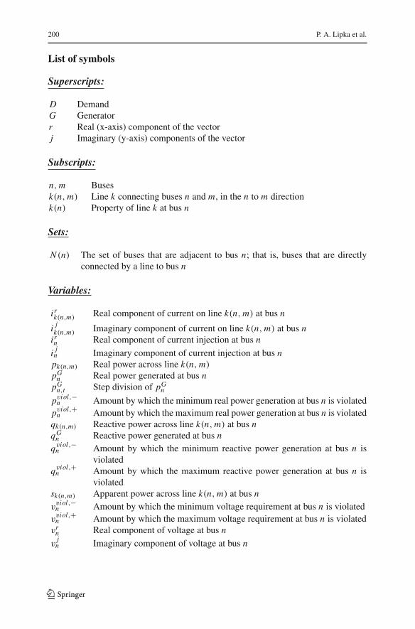
List of symbols

Superscripts:

D DemandG Generatorr Real (x-axis) component of the vectorj Imaginary (y-axis) components of the vector

Subscripts:

n,m Busesk(n,m) Line k connecting buses n and m, in the n to m directionk(n) Property of line k at bus n

Sets:

N (n) The set of buses that are adjacent to bus n; that is, buses that are directlyconnected by a line to bus n

Variables:

irk(n,m) Real component of current on line k(n,m) at bus n

i jk(n,m) Imaginary component of current on line k(n,m) at bus nirn Real component of current injection at bus n

i jn Imaginary component of current injection at bus npk(n,m) Real power across line k(n,m)

pGn Real power generated at bus npGn,t Step division of pGnpviol,−n Amount by which the minimum real power generation at bus n is violatedpviol,+n Amount by which the maximum real power generation at bus n is violatedqk(n,m) Reactive power across line k(n,m) at bus nqGn Reactive power generated at bus nqviol,−n Amount by which the minimum reactive power generation at bus n is

violatedqviol,+n Amount by which the maximum reactive power generation at bus n is

violatedsk(n,m) Apparent power across line k(n,m) at bus nvviol,−n Amount by which the minimum voltage requirement at bus n is violatedvviol,+n Amount by which the maximum voltage requirement at bus n is violatedvrn Real component of voltage at bus n

vjn Imaginary component of voltage at bus n

123

Constructing transmission line current constraints... 201

Parameters:

fn Cost coefficient on the square of pGn in MATPOWERen Cost coefficient on pGn in MATPOWERcn,pen Penalty cost of violating constraints at bus ncn,t Step-cost of real power at bus n at step tbk(n) Electrical susceptance of transmission line k at bus ngk(n) Electrical conductance of transmission line k at bus nimaxk(n,m) Maximum allowed current on line k(n,m)

pDn Real power demand at bus nqDn Reactive power demand at bus npminn Minimum required real power at bus n

pmaxn Maximum allowed real power at bus n

pG,stepn Step size for real power; equals pmax

n −pminn

Tqminn Minimum required reactive power at bus n

qmaxn Maximum allowed reactive power at bus nvminn Minimum required voltage magnitude at bus nvmaxn Maximum allowed voltage magnitude at bus nT Total number of steps for the stepwise approximationt Index of the step; t =1, 2, …,T

1 Introduction

The amount of current that can flow through power system transmission lines is limitedby thermal restrictions. The thermal ratings of the transmission lines depend on thematerials that compose them and environmental conditions. Heat loss on the line isproportional to the magnitude of the line’s current squared. If the line current exceedsthe recommended limit for too long, the excessive heat caused by the line current candeform and degrade transmission lines and cause them to sag. Limiting current is themost direct measurement to limit the temperature of the line; however, this thermallimit is often converted to a limit on apparent or real power as it is easier to representin traditional optimal power flow (OPF) formulations that consider the variables ofvoltage and power but not current. Additionally, current and other line limits may beimposed to enforce stability.

The IEEE test systems [5] and Polish systems [20] are commonly used to test newalgorithms for solving power flow problems. However, no IEEE test problems includecurrent magnitude limits on the transmission lines, and many of the test systemsinclude no thermal limits at all, including the 14-, 57-, 118-, and 300-bus systems.If a test problem does not include these limits, reasonable constraints may need tobe created for testing purposes. Solving an OPF problem is often difficult due to theline limits; testing algorithms on cases without line limits does not provide a goodrepresentation on how the algorithm will work in practice. In MATPOWER [20], the30-bus system contains apparent power limits on lines; these constraints do not causemuch congestion and do not give much insight into a stressed system. The larger test

123

202 P. A. Lipka et al.

cases do contain line limits; however, these limits need to be converted from being alimit on apparent power to a limit on current.

In the absence of thermal constraints, such as in the 14- to 300-bus systems, oneapproach is to create constraints based on the physical characteristics and expectedenvironmental conditions. Often, there is little information available about the lines. Ittakes considerable time to develop constraints based on physical characteristics, andthe result may not be binding constraints.

The purpose of this paper is to develop a methodology for creating constraintson the line current magnitude using a set of the IEEE test problems and to establishstandard limits that can be used in the testing of power flow algorithms. Bindingconstraints based onmaximumcurrentmagnitude are created rather than on constraintson apparent power on the lines or on voltage angle differences.

For systems without limits, the proposed approach is to create constraints fromthe optimal solution (with no line limits imposed). Subsequent testing explores howmodifying the line limits, created from the solution of the non-constrained problem,affects the resulting power flow solution. For the Polish systems containing thermallimits, the apparent power limits are converted to current limits. Two types of lineconstraints are proposed for the test systems. The “tight” constraint level restrictscurrent on lines to a lower amount than the “loose” constraint level. This paper hasessentially created new power system test cases that provide current limits on the lines.

The rest of the paper is organized as follows: the background of theACOPFproblemand how line constraints work is discussed in Sect. 2. Section 3 describes the approachto the formulation used and how the line constraints are constructed. Numerical resultsand the recommended line limits are given in Sect. 4. The paper is summarized inSect. 5.

2 Background

This section discusses the history of the power flow problem, the standard for estab-lishing current limits, and the relationship between the different line limits.

2.1 AC power flow problem

The power flow problem provides network solutions, such as bus voltage magnitudesand angles, for a given set of conditions. The optimal power flow (OPF) probleminvolves executing these requirements at maximum market surplus. If demand isconsidered inelastic, maximizing market surplus is equivalent to minimizing powerprocurement costs. Power networks have buses that are connected by lines with bothresistance and reactance, so these power flow problems are generally designated asalternating current optimal power flow (ACOPF) problems. Independent SystemOper-ators (ISOs) and Regional Transmission Organizations (RTOs) in the United Statesand Canada run power markets based on optimal power flow over large regions. Sincethese markets are so large and the dispatch time is typically 5 min, these organiza-tions generally run the direct current (DC) approximation of the ACOPF with somemodifications in order to find a solution within the time window.

123

Constructing transmission line current constraints... 203

While the alternating current optimal power flow problem has been studied forover 50 years [4], no single approach has been permanently settled on. The ACOPFis nonlinear and nonconvex, which makes it hard to find a feasible solution and evenharder to find one that is the global solution. There are many approaches to solv-ing this problem. These include Newton methods [16–18], interior point algorithms[10–17], semidefinite relaxations [11,12,14], conic approaches [9], and direct currentapproximations. As many theoretically good algorithms may run into trouble duringimplementation, the different methods and approximations used to solve the OPF areextensively tested on sample data.

2.2 Current line limits standards

Transmission line limits used in solving power flow problems include limits on realpower, voltage angle difference, apparent power, and current. The IEEE standard [1]suggests calculating a thermal limit on current based on environmental conditions andmaterial properties. Transmission lines generally have maximum temperature ratings.These include a normal and emergency rating, and these ratings typically depend onthe characteristics of the conductor material. Resistance of a line is dependent ontemperature; increasing the temperature increases the resistance. Since the IEEE testsystems included only steady-state data, the current limits are also derived at steady-state. While there are many different ways to calculate maximum current, the IEEEStandard 738 , shown in (1), provides one well-accepted method.

imax =√qc + qr − qs

R(TC )(1)

In the IEEEStandard 738, qc is the convected heat loss, qr is the radiated heat loss, qs isthe solar heat gain, and R(TC ) is the resistance of the line per length at temperature TC .The physical properties that increase the current line limit include a higher maximumtemperature rating, larger diameter, and higher emissivity. The environmental factorsthat increase this limit include a higher wind speed, a lower ambient temperature,and less direct sun. The IEEE test systems present part of the Midwest electric grid.While Bockarjova and Andersson [3] derived current line constraints on the IEEE14-bus system using the IEEE 738 Standard; however, they had to make extensiveassumptions about the network characteristics and environmental conditions in orderto use the IEEE standard. The data needed to compute line limits from the IEEEstandards is not available. One would need the diameter of the lines, their maximumtemperature ratings, ambient temperature, line length, and many more parameters thatare not given. Therefore, this paper examines creating line limits based on findinglimits that bind rather than trying to derive them from physical properties.

2.3 Converting apparent power limits to current limits

The limits on real power and voltage angle differences are most often used whensolving a DC approximation of the ACOPF as reactive power is neglected in the

123

204 P. A. Lipka et al.

DCOPF. Limits on apparent power, as shown in (5)–(6), or current (7) are often usedwhen solving the AC power flow formulation. A limit on apparent power or real poweris often used for line limits for the power-voltage formulation of the ACOPF, and alimit on current is often used for the current-voltage formulation.

While all of the different limits have the impact of preventing temperature on thelines from becoming too large, the different limits are not equivalent.

pk(n,m) = irk(n,m)

(vrn − vrm

) + i jk(n,m)

(vjn − v

jm

)(2)

qk(n,m) = irk(n,m)

(vjn − v

jm

)+ i jk(n,m)

(−vrn + vrm)

(3)

sk(n,m) = pk(n,m) + jqk(n,m) (4)

|sk(n,m)| =√p2k(n,m) + q2k(n,m) (5)

s2k(n,m) = v2ni2nmk (6)

Given a limit on the apparent power on the line, the equivalent limit on the currentflow on the line can be bounded, as shown in (7).

smaxk(n,m)

vmaxn

≤ imaxk(n,m) ≤ smax

k(n,m)

vminn

(7)

3 Methodology

For the IEEE problems, the problems are solved without line constraints, and tight andloose limits are created based on restricting current below the highest current whenthe OPF was solved. Section 3.1 gives the formulation that is used to solve for theoptimal power flow, and Sect. 3.2 describes how the IEEE line limits are set. Section3.3 shows how the apparent power limits of the Polish systems are converted to currentlimits using the bounds on current flow given in (7).

3.1 Formulation

Here, the current-voltage formulation of the ACOPF, first discussed in [6] and usedto solve power flow in [7] is used to consider the different current constraints. Alter-natively, the current constraints could be added to other formulations of the ACOPF,such as the polar or rectangular voltage-based formulations.

The cost function used by MATPOWER [20] is a quadratic function.

Cost =∑n

fn(pGn

)2 + en(pGn

)(8)

However, most ISOs and RTOs accept power bids as step functions rather than thesmooth cost. Therefore, the objective considered is the piecewise linear function thatapproximates the quadratic function. To find this approximation, the amount of realpower supplied is broken up into T equal pieces. Since the real power is bounded above

123

Constructing transmission line current constraints... 205

0 1 2 3 4 5 60

20

40

60

80

100

120

Real Power Generated

Rea

l Pow

er C

ost

MATPOWER Cost

Piecewise Linear Cost

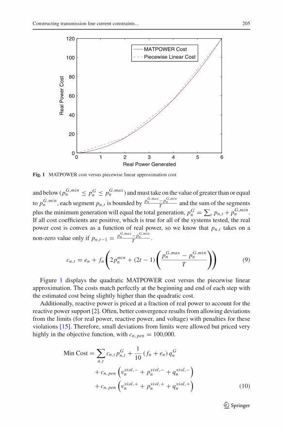
Fig. 1 MATPOWER cost versus piecewise linear approximation cost

andbelow (pG,minn ≤ pGn ≤ pG,max

n ) andmust take on the value of greater thanor equal

to pG,minn , each segment pn,t is bounded by

pG,maxn −pG,min

nT and the sum of the segments

plus the minimum generation will equal the total generation, pGn = ∑t pn,t + pG,min

n .If all cost coefficients are positive, which is true for all of the systems tested, the realpower cost is convex as a function of real power, so we know that pn,t takes on a

non-zero value only if pn,t−1 = pG,maxn −pG,min

nT .

cn,t = en + fn

(2pmin

n + (2t − 1)

(pG,maxn − pG,min

n

T

))(9)

Figure 1 displays the quadratic MATPOWER cost versus the piecewise linearapproximation. The costs match perfectly at the beginning and end of each step withthe estimated cost being slightly higher than the quadratic cost.

Additionally, reactive power is priced at a fraction of real power to account for thereactive power support [2]. Often, better convergence results from allowing deviationsfrom the limits (for real power, reactive power, and voltage) with penalties for theseviolations [15]. Therefore, small deviations from limits were allowed but priced veryhighly in the objective function, with cn,pen = 100,000.

Min Cost =∑n,t

cn,t pGn,t + 1

10( fn + en) q

Gn

+ cn,pen(vviol,−n + pviol,−n + qviol,−n

)

+ cn,pen(vviol,+n + pviol,+n + qviol,+n

)(10)

123

206 P. A. Lipka et al.

such that:

irk(n,) = gk(n)vrn − gk(m)v

rm − bk(n)v

jn + bk(m)v

jm (11)

i jk(n,m) = bk(n)vrn − bk(m)v

rm + gk(n)v

jn − gk(m)v

jm (12)

irn =∑

m∈N (n)

irk(n,m) (13)

i jn =∑

m∈N (n)

i jk(n,m) (14)

− vviol,−n +(vminn

)2 ≤ (vrn

)2 +(vjn

)2 ≤ (vmaxn

)2 + vviol,+n (15)(irk(n,m)

)2 +(i jk(n,m)

)2 ≤(imaxk(n,m)

)2(16)

pGn = vrnirn + v

jn i

jn + pDn (17)

pGn = pminn +

∑t

pGn,t (18)

0 ≤ pn,t ≤ pG,stepn (19)

qGn = vjn i

rn − vrni

jn + qD

n (20)

− pviol,−n + pG,minn ≤ pGn ≤ pG,max

n + pviol,+n (21)

− pviol,−n + pD,minn ≤ pDn ≤ pD,max

n + pviol,+n (22)

− qviol,−n + qG,minn ≤ qGn ≤ qG,max

n + qviol,+n (23)

− qviol,−n + qD,minn ≤ qD

n ≤ qD,maxn + qviol,+n (24)

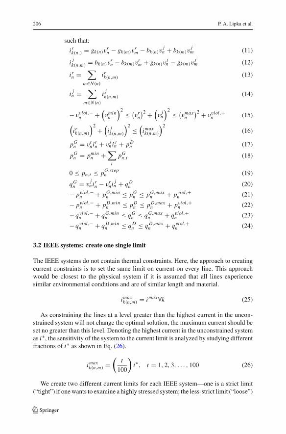
3.2 IEEE systems: create one single limit

The IEEE systems do not contain thermal constraints. Here, the approach to creatingcurrent constraints is to set the same limit on current on every line. This approachwould be closest to the physical system if it is assumed that all lines experiencesimilar environmental conditions and are of similar length and material.

imaxk(n,m) = imax∀k (25)

As constraining the lines at a level greater than the highest current in the uncon-strained system will not change the optimal solution, the maximum current should beset no greater than this level. Denoting the highest current in the unconstrained systemas i∗, the sensitivity of the system to the current limit is analyzed by studying differentfractions of i∗ as shown in Eq. (26).

imaxk(n,m) =

(t

100

)i∗, t = 1, 2, 3, . . . , 100 (26)

We create two different current limits for each IEEE system—one is a strict limit(“tight”) if onewants to examine a highly stressed system; the less-strict limit (“loose”)

123

Constructing transmission line current constraints... 207

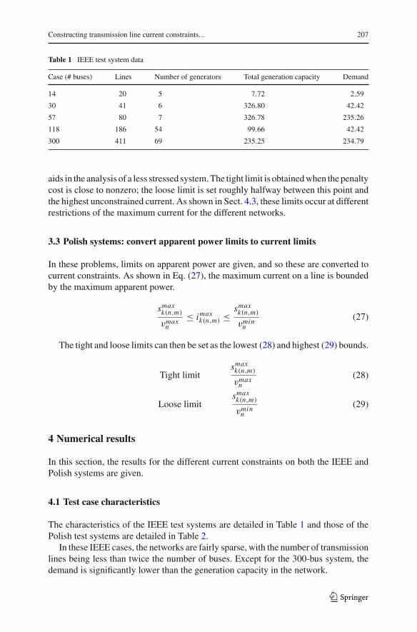
Table 1 IEEE test system data

Case (# buses) Lines Number of generators Total generation capacity Demand

14 20 5 7.72 2.59

30 41 6 326.80 42.42

57 80 7 326.78 235.26

118 186 54 99.66 42.42

300 411 69 235.25 234.79

aids in the analysis of a less stressed system.The tight limit is obtainedwhen the penaltycost is close to nonzero; the loose limit is set roughly halfway between this point andthe highest unconstrained current. As shown in Sect. 4.3, these limits occur at differentrestrictions of the maximum current for the different networks.

3.3 Polish systems: convert apparent power limits to current limits

In these problems, limits on apparent power are given, and so these are converted tocurrent constraints. As shown in Eq. (27), the maximum current on a line is boundedby the maximum apparent power.

smaxk(n,m)

vmaxn

≤ imaxk(n,m) ≤ smax

k(n,m)

vminn

(27)

The tight and loose limits can then be set as the lowest (28) and highest (29) bounds.

Tight limitsmaxk(n,m)

vmaxn

(28)

Loose limitsmaxk(n,m)

vminn

(29)

4 Numerical results

In this section, the results for the different current constraints on both the IEEE andPolish systems are given.

4.1 Test case characteristics

The characteristics of the IEEE test systems are detailed in Table 1 and those of thePolish test systems are detailed in Table 2.

In these IEEE cases, the networks are fairly sparse, with the number of transmissionlines being less than twice the number of buses. Except for the 300-bus system, thedemand is significantly lower than the generation capacity in the network.

123

208 P. A. Lipka et al.

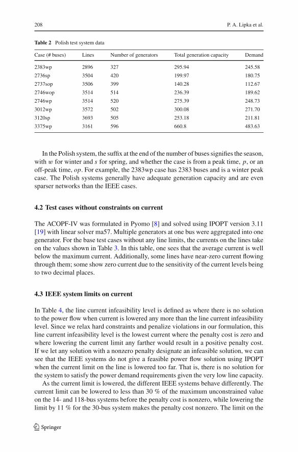
Table 2 Polish test system data

Case (# buses) Lines Number of generators Total generation capacity Demand

2383wp 2896 327 295.94 245.58

2736sp 3504 420 199.97 180.75

2737sop 3506 399 140.28 112.67

2746wop 3514 514 236.39 189.62

2746wp 3514 520 275.39 248.73

3012wp 3572 502 300.08 271.70

3120sp 3693 505 253.18 211.81

3375wp 3161 596 660.8 483.63

In the Polish system, the suffix at the end of the number of buses signifies the season,with w for winter and s for spring, and whether the case is from a peak time, p, or anoff-peak time, op. For example, the 2383wp case has 2383 buses and is a winter peakcase. The Polish systems generally have adequate generation capacity and are evensparser networks than the IEEE cases.

4.2 Test cases without constraints on current

The ACOPF-IV was formulated in Pyomo [8] and solved using IPOPT version 3.11[19] with linear solver ma57. Multiple generators at one bus were aggregated into onegenerator. For the base test cases without any line limits, the currents on the lines takeon the values shown in Table 3. In this table, one sees that the average current is wellbelow the maximum current. Additionally, some lines have near-zero current flowingthrough them; some show zero current due to the sensitivity of the current levels beingto two decimal places.

4.3 IEEE system limits on current

In Table 4, the line current infeasibility level is defined as where there is no solutionto the power flow when current is lowered any more than the line current infeasibilitylevel. Since we relax hard constraints and penalize violations in our formulation, thisline current infeasibility level is the lowest current where the penalty cost is zero andwhere lowering the current limit any farther would result in a positive penalty cost.If we let any solution with a nonzero penalty designate an infeasible solution, we cansee that the IEEE systems do not give a feasible power flow solution using IPOPTwhen the current limit on the line is lowered too far. That is, there is no solution forthe system to satisfy the power demand requirements given the very low line capacity.

As the current limit is lowered, the different IEEE systems behave differently. Thecurrent limit can be lowered to less than 30 % of the maximum unconstrained valueon the 14- and 118-bus systems before the penalty cost is nonzero, while lowering thelimit by 11 % for the 30-bus system makes the penalty cost nonzero. The limit on the

123

Constructing transmission line current constraints... 209

Table 3 Unconstrained current levels, in p.u.

System (# buses) Min. current Avg. current Max. current

14 0.02 0.28 1.14

30 0.00 0.12 0.35

57 0.01 0.22 1.77

118 0.00 0.44 4.02

300 0.01 1.316 10.820

2383wp 0.00 0.36 8.83

2736sp 0.00 0.26 4.81

2737sop 0.00 0.17 3.66

2746wop 0.00 0.27 6.44

2746wp 0.00 0.32 6.22

3012wp 0.00 0.35 8.66

3120sp 0.00 0.31 9.07

3375wp 0.00 0.52 10.00

Table 4 Current level belowwhich the penalty cost is >0 forthis limit on all lines

No. of buses Line current infeasibilitylevel (p.u.)

Percent of i∗

14 0.227 20

30 0.309 89

57 1.408 80

118 1.136 28

300 6.780 63

300-bus system can be lowered to 63 % of its original level before there are problemsfinding a feasible solution.

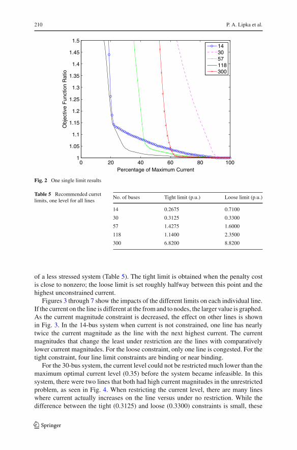
Figure 2 plots the ratio of the constrained system’s objective function (includingpenalty costs) to the unconstrained system’s objective function on the y axis and thefraction of the maximum unconstrained current that is set as the current maximum onthe x-axis (the value of t in (26)). The point where the curve becomes an asymptote iswhere the system becomes infeasible. Reducing the current limit has different effectson the different systems. Examining the ratio of the constrained objective functionto the unconstrained objective function, the highest objective function for the 14-bussystem with a zero-penalty solution is 26 % higher than the unconstrained objectivevalue; for the 30-bus system, it is only 1.7 % higher. The objective function for the57-bus system is only 0.004 % higher; the 118-bus system has more difference withthe objective function being 5.3 % higher than the unconstrained function. For the300-bus system, the objective function at the lowest current limit before the system isinfeasible is 0.8 % higher than with no limits on current.

Two levels of current limits are suggested—one is a strict limit (“tight”) if onewantsto examine a highly stressed system; the non-strict limit (“loose”) aids in the analysis

123

210 P. A. Lipka et al.

0 20 40 60 80 1001

1.05

1.1

1.15

1.2

1.25

1.3

1.35

1.4

1.45

1.5

Percentage of Maximum Current

Obj

ectiv

e F

unct

ion

Rat

io

143057118300

Fig. 2 One single limit results

Table 5 Recommended curretlimits, one level for all lines

No. of buses Tight limit (p.u.) Loose limit (p.u.)

14 0.2675 0.7100

30 0.3125 0.3300

57 1.4275 1.6000

118 1.1400 2.3500

300 6.8200 8.8200

of a less stressed system (Table 5). The tight limit is obtained when the penalty costis close to nonzero; the loose limit is set roughly halfway between this point and thehighest unconstrained current.

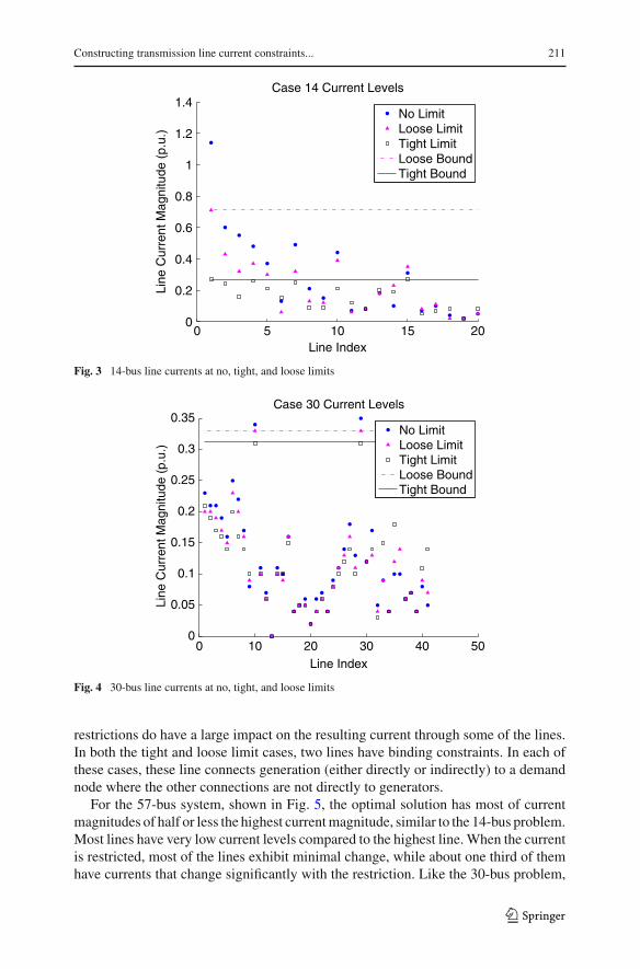
Figures 3 through 7 show the impacts of the different limits on each individual line.If the current on the line is different at the fromand to nodes, the larger value is graphed.As the current magnitude constraint is decreased, the effect on other lines is shownin Fig. 3. In the 14-bus system when current is not constrained, one line has nearlytwice the current magnitude as the line with the next highest current. The currentmagnitudes that change the least under restriction are the lines with comparativelylower current magnitudes. For the loose constraint, only one line is congested. For thetight constraint, four line limit constraints are binding or near binding.

For the 30-bus system, the current level could not be restricted much lower than themaximum optimal current level (0.35) before the system became infeasible. In thissystem, there were two lines that both had high current magnitudes in the unrestrictedproblem, as seen in Fig. 4. When restricting the current level, there are many lineswhere current actually increases on the line versus under no restriction. While thedifference between the tight (0.3125) and loose (0.3300) constraints is small, these

123

Constructing transmission line current constraints... 211

0 5 10 15 200

0.2

0.4

0.6

0.8

1

1.2

1.4

Line Index

Line

Cur

rent

Mag

nitu

de (

p.u.

)

Case 14 Current Levels

No LimitLoose LimitTight LimitLoose BoundTight Bound

Fig. 3 14-bus line currents at no, tight, and loose limits

0 10 20 30 40 500

0.05

0.1

0.15

0.2

0.25

0.3

0.35

Line Index

Line

Cur

rent

Mag

nitu

de (

p.u.

)

Case 30 Current Levels

No LimitLoose LimitTight LimitLoose BoundTight Bound

Fig. 4 30-bus line currents at no, tight, and loose limits

restrictions do have a large impact on the resulting current through some of the lines.In both the tight and loose limit cases, two lines have binding constraints. In each ofthese cases, these line connects generation (either directly or indirectly) to a demandnode where the other connections are not directly to generators.

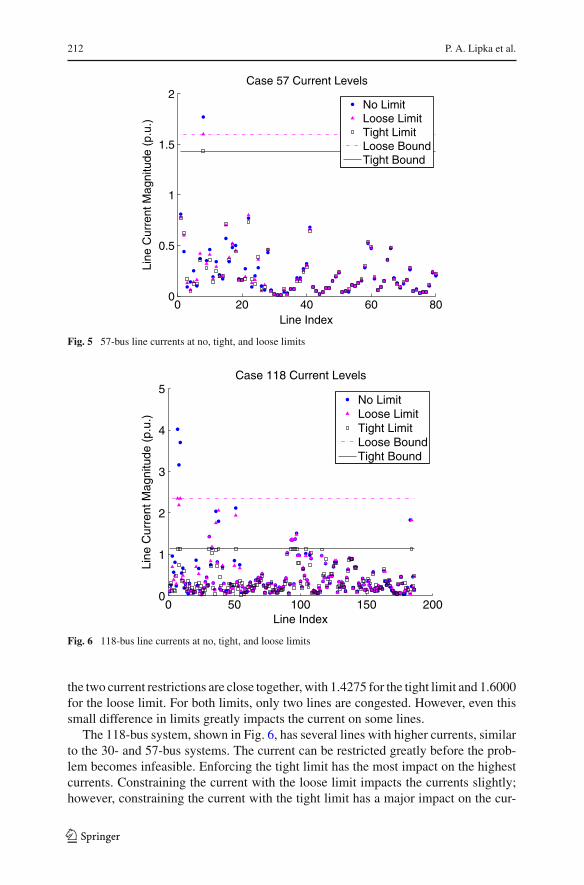
For the 57-bus system, shown in Fig. 5, the optimal solution has most of currentmagnitudes of half or less the highest currentmagnitude, similar to the 14-bus problem.Most lines have very low current levels compared to the highest line.When the currentis restricted, most of the lines exhibit minimal change, while about one third of themhave currents that change significantly with the restriction. Like the 30-bus problem,

123

212 P. A. Lipka et al.

0 20 40 60 800

0.5

1

1.5

2

Line Index

Line

Cur

rent

Mag

nitu

de (

p.u.

)

Case 57 Current Levels

No LimitLoose LimitTight LimitLoose BoundTight Bound

Fig. 5 57-bus line currents at no, tight, and loose limits

0 50 100 150 2000

1

2

3

4

5

Line Index

Line

Cur

rent

Mag

nitu

de (

p.u.

)

Case 118 Current Levels

No LimitLoose LimitTight LimitLoose BoundTight Bound

Fig. 6 118-bus line currents at no, tight, and loose limits

the two current restrictions are close together, with 1.4275 for the tight limit and 1.6000for the loose limit. For both limits, only two lines are congested. However, even thissmall difference in limits greatly impacts the current on some lines.

The 118-bus system, shown in Fig. 6, has several lines with higher currents, similarto the 30- and 57-bus systems. The current can be restricted greatly before the prob-lem becomes infeasible. Enforcing the tight limit has the most impact on the highestcurrents. Constraining the current with the loose limit impacts the currents slightly;however, constraining the current with the tight limit has a major impact on the cur-

123

Constructing transmission line current constraints... 213

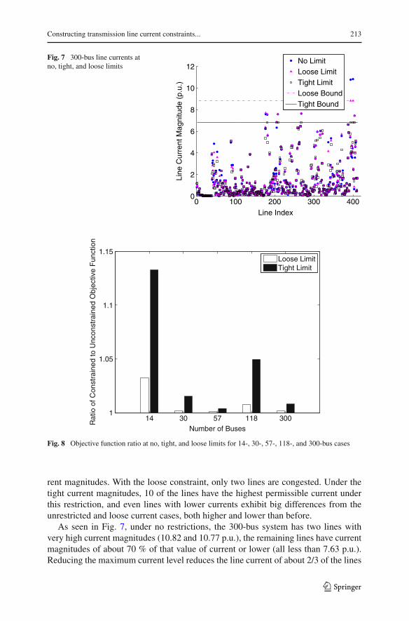
Fig. 7 300-bus line currents atno, tight, and loose limits

0 100 200 300 4000

2

4

6

8

10

12

Line Index

Line

Cur

rent

Mag

nitu

de (

p.u.

)

No LimitLoose LimitTight LimitLoose BoundTight Bound

14 30 57 118 3001

1.05

1.1

1.15

Number of Buses

Rat

io o

f Con

stra

ined

to U

ncon

stra

ined

Obj

ectiv

e F

unct

ion

Loose LimitTight Limit

Fig. 8 Objective function ratio at no, tight, and loose limits for 14-, 30-, 57-, 118-, and 300-bus cases

rent magnitudes. With the loose constraint, only two lines are congested. Under thetight current magnitudes, 10 of the lines have the highest permissible current underthis restriction, and even lines with lower currents exhibit big differences from theunrestricted and loose current cases, both higher and lower than before.

As seen in Fig. 7, under no restrictions, the 300-bus system has two lines withvery high current magnitudes (10.82 and 10.77 p.u.), the remaining lines have currentmagnitudes of about 70 % of that value of current or lower (all less than 7.63 p.u.).Reducing the maximum current level reduces the line current of about 2/3 of the lines

123

214 P. A. Lipka et al.

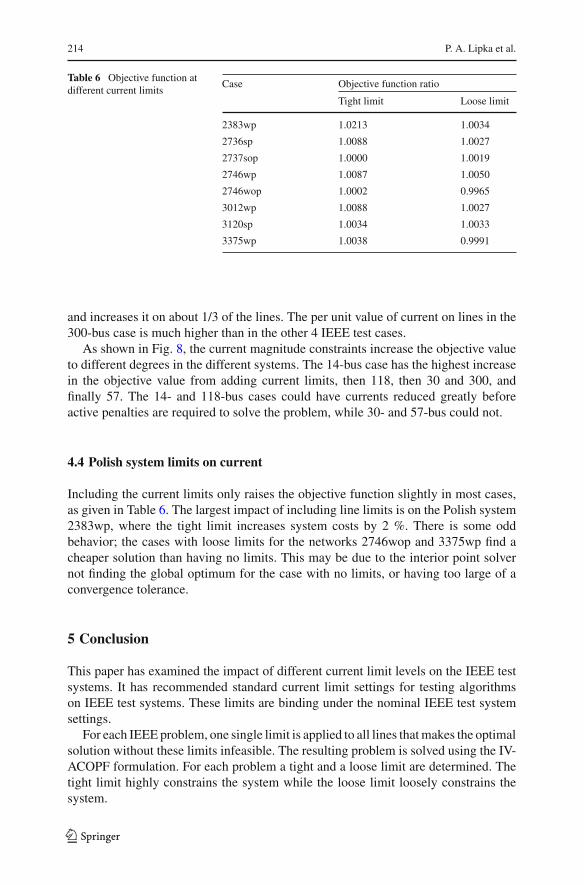
Table 6 Objective function atdifferent current limits

Case Objective function ratio

Tight limit Loose limit

2383wp 1.0213 1.0034

2736sp 1.0088 1.0027

2737sop 1.0000 1.0019

2746wp 1.0087 1.0050

2746wop 1.0002 0.9965

3012wp 1.0088 1.0027

3120sp 1.0034 1.0033

3375wp 1.0038 0.9991

and increases it on about 1/3 of the lines. The per unit value of current on lines in the300-bus case is much higher than in the other 4 IEEE test cases.

As shown in Fig. 8, the current magnitude constraints increase the objective valueto different degrees in the different systems. The 14-bus case has the highest increasein the objective value from adding current limits, then 118, then 30 and 300, andfinally 57. The 14- and 118-bus cases could have currents reduced greatly beforeactive penalties are required to solve the problem, while 30- and 57-bus could not.

4.4 Polish system limits on current

Including the current limits only raises the objective function slightly in most cases,as given in Table 6. The largest impact of including line limits is on the Polish system2383wp, where the tight limit increases system costs by 2 %. There is some oddbehavior; the cases with loose limits for the networks 2746wop and 3375wp find acheaper solution than having no limits. This may be due to the interior point solvernot finding the global optimum for the case with no limits, or having too large of aconvergence tolerance.

5 Conclusion

This paper has examined the impact of different current limit levels on the IEEE testsystems. It has recommended standard current limit settings for testing algorithmson IEEE test systems. These limits are binding under the nominal IEEE test systemsettings.

For each IEEEproblem, one single limit is applied to all lines thatmakes the optimalsolution without these limits infeasible. The resulting problem is solved using the IV-ACOPF formulation. For each problem a tight and a loose limit are determined. Thetight limit highly constrains the system while the loose limit loosely constrains thesystem.

123

Constructing transmission line current constraints... 215

For the 14-, 30-, 57-, 118-, and 300-bus problems, creating line current magnitudeconstraints for the ACOPF problem can result in problems that may be infeasible.As one tightens the current magnitude constraints, the objective function increasesgradually at first, then increases exponentially once penalties are required to solve theproblem. Different test problems exhibit different characteristics in the line currentmagnitude distribution and at what current magnitude level constraint the problembecomes infeasible. The Polish systems exhibit small changes between the constrainedand unconstrained systems.

Acknowledgements This work was partially supported by a National Science Foundation GraduateResearch Fellowship, DGE 1106400 and by the US Department of Energy under an Advanced ResearchProjects Agency-Energy/Green Electricity Network Integration (ARPA-E/GENI) contract. Initial ground-work for this paper is based on work done for a Federal Energy Regulatory Commission Staff Paper [13].

References

1. IEEE standard for calculating the current-temperature of bare overhead conductors. IEEE Std. 738-2006 (2006)

2. Baughman, M., Siddiqi, S.: Real-time pricing of reactive power: theory and case study results. IEEETrans. Power Syst. 6(1), 23–29 (1991). doi:10.1109/59.131043

3. Bockarjova, M., Andersson, G.: Transmission line conductor temperature impact on state estimationaccuracy. In: IEEE Lausanne Power Tech 2007, pp. 701–706. IEEE (2007)

4. Carpentier, J.: Contribution to the economic dispatch problem. Bulletin de la Societe Francoise desElectriciens 3(8), 431–447 (1962)

5. Christie, R.: Power systems test case archive. University of Washington, Department of ElectricalEngineering [Online]. Available: http://www.ee.washington.edu/research/pstca/ (1993)

6. Dommel, H., Tinney, W., Powell, W.: Further developments in Newton’s method for power systemapplications. In: IEEE Winter Power Meeting, Conference Paper, vol. 70 (1970)

7. Exposito, A., Ramos, E.: Augmented rectangular load flow model. IEEE Trans. Power Syst. 17(2),271–276 (2002). doi:10.1109/TPWRS.2002.1007892

8. Hart, W.E., Watson, J.P., Woodruff, D.L.: Pyomo: modeling and solving mathematical programs inPython. Math. Program. Comput. 3(3), 219–260 (2011)

9. Jabr, R.A.: Optimal power flow using an extended conic quadratic formulation. IEEE Trans. PowerSyst. 23(3), 1000–1008 (2008)

10. Jiang, Q., Geng, G., Guo, C., Cao, Y.: An efficient implementation of automatic differentiation ininterior point optimal power flow. IEEE Trans. Power Syst. 25(1), 147–155 (2010)

11. Lavaei, J., Low, S.H.: Zero duality gap in optimal power flow problem. IEEE Trans. Power Syst. 27(1),92–107 (2012)

12. Lesieutre, B.C., Molzahn, D.K., Borden, A.R., DeMarco, C.L.: Examining the limits of the applicationof semidefinite programming to power flow problems. In: 2011 49th Annual Allerton Conference onCommunication, Control, and Computing (Allerton), pp. 1492–1499. IEEE (2011)

13. Lipka, P., O’Neill, R., Oren, S.: Developing line current magnitude constraints for IEEEtest problems (2013). http://www.ferc.gov/industries/electric/indus-act/market-planning/opf-papers/acopf-7-line-constraints

14. Molzahn, D., Holzer, J., Lesieutre, B., DeMarco, C.: Implementation of a large-scale optimal powerflow solver based on semidefinite programming. IEEE Trans. Power Syst. 28(4), 3987–3998 (2013).doi:10.1109/TPWRS.2013.2258044

15. Ramamoorty, M., Gopala Rao, J.: Economic load scheduling of thermal power systems using thepenalty function approach. IEEE Trans. Power Apparatus Syst. 89(8), 2075–2078 (1970). doi:10.1109/TPAS.1970.292793

16. Rashed, A., Kelly, D.: Optimal load flow solution using lagrangian multipliers and the hessian matrix.IEEE Trans. Power Apparatus Syst. 5, 1292–1297 (1974)

17. Sousa, A.A., Torres, G.L., Cañizares, C.A.: Robust optimal power flow solution using trust region andinterior-point methods. IEEE Trans. Power Syst. 26(2), 487–499 (2011)

123

216 P. A. Lipka et al.

18. Sun, D.I., Ashley, B., Brewer, B., Hughes, A., Tinney, W.F.: Optimal power flow by newton approach.IEEE Trans. Power Apparatus Syst. 10, 2864–2880 (1984)

19. Wächter, A., Biegler, L.T.: On the implementation of an interior-point filter line-search algorithm forlarge-scale nonlinear programming. Math. Program. 106(1), 25–57 (2006)

20. Zimmerman, R.D., Murillo-Sánchez, C.E., Thomas, R.J.: MATPOWER: steady-state operations, plan-ning, and analysis tools for power systems research and education. IEEE Trans. Power Syst. 26(1),12–19 (2011)

123