Constraint Programming Approach to a Bilevel

Scheduling Problem

Andras Kovacs, Tamas KisComputer and Automation Research Institute

Hungarian Academy of SciencesE-mail addresses: {andras.kovacs,tamas.kis}@sztaki.hu

March 4, 2010

Abstract

Bilevel optimization problems involve two decision makers who maketheir choices sequentially, either one according to its own objective func-tion. Many problems arising in economy and management science can bemodeled as bilevel optimization problems. Several special cases of bilevelproblem have been studied in the literature, e.g., linear bilevel problems.However, up to now, very little is known about solution techniques ofdiscrete bilevel problems. In this paper we show that constraint program-ming can be used to model and solve such problems. We demonstrate ourfirst results on a simple bilevel scheduling problem.

Keywords: Scheduling, bilevel programming, constraint modeling, QCSP

1 Introduction

Bilevel programming deals with decision and optimization problems whose out-come is determined by the interplay of two self-interested decision makers whodecide sequentially. First, the decision maker called the leader makes its choice.Then, in view of the leader’s decision, the follower chooses its response. Eitherdecision maker aims at minimizing (maximizing) its own objective function. Inthe general case, the objective values mutually depend on the choices of theother party. Technically, the follower’s role can be seen as solving a parametricoptimization problem, whose parameters are determined by the leader. Theparticularly interesting situation is that of the leader, who is assumed to havea complete knowledge of the follower’s constraints, objective, and input data.He endeavors to find his best choice subject to the response that he can expectfrom the self-interested follower. In the optimistic (pessimistic) case the leaderassumes that the follower chooses from the set of its optimal responses the onethat is the most (least) favorable for the leader.

1

Formally, the set of all variables in the problem is partitioned into two sets:the leader’s variables X, and the follower’s variables Y . The leader can assignvalues to X, while the follower decides about Y , and it is assumed that allvariables have finite domains. The leader aims at minimizing f subject to theconstraint set C and the follower’s optimality condition, which states that thefollower will minimize g subject to D. Also, the leader must avoid the values ofX for which the follower’s response does not satisfy C. Throughout the paper weassume that both the leader and the follower try to minimize their objectives,though, the same techniques can be used for maximization or mixed problemsas well. Hence, the optimistic bilevel problem can be formulated as:

minX,Y

f(X,Y ) (1)

subject toC(X,Y ) (2)Y ∈ arg min

Y ′(g(X,Y ′) | D(X,Y ′)) (3)

In formula (3), the operator arg min refers to the set of all optimal solutions ofthe problem at hand. Moreover, the pessimistic case of the problem is describedas:

minX

maxY

f(X,Y ) (4)

subject toC(X,Y ) (5)Y ∈ arg min

Y ′(g(X,Y ′) | D(X,Y ′)). (6)

Bilevel programming techniques can be applied to model various decisionproblems of actors in customer-producer relations, in competition, or at variouslevels of an organizational hierarchy. Despite this, well-founded theoretical re-sults are known for special cases of bilevel problems only. These include variousexact and heuristic approaches to linear bilevel problems (where all constraintsand both objective functions are linear expressions over continuous variables),and mostly heuristic methods for other cases, such as bilinear problems [13].The papers [12, 14] address problems where the follower’s variables can takediscrete values. For (fully) discrete bilevel problems, which are in the focus ofthis study, only sporadic application results are available, see [22, 26]. Also, tothe best of our knowledge, this paper is the first to investigate the solution ofbilevel optimization problems using constraint programming (CP) techniques.

1.1 A motivating example

The classical approach in management science assumes that the different de-partments of the same company, although have individual decision roles and

2

responsibilities, subsume their interest to the same global objective. This ob-jective is related to maximizing the long-term profit of the company. The realityis often different: the performance of each department is evaluated using, andrewarded based on, a different performance measure. These performance mea-sures are only distantly related to the global objective of the company, and areoften conflicting. Hence, a relevant alternative model of the joint operation ofseveral departments is using multilevel programming techniques [4]. A simplecase study is presented below.

Consider the bilevel scheduling problem where the management of the com-pany (the leader) is responsible for order acceptance and the workshop foreman(the follower) decides on the execution sequence of the tasks corresponding toaccepted orders. The leader has no direct influence on the sequencing decisions.Formally, there is a set of tasks T , some of which will have to be scheduled on asingle unary resource. Task j is characterized by its processing time pj , releasetime rj , and deadline dj . The difference between the profit if j is executed ontime and the loss of reputation if it is rejected is captured by the cost (or taskweight) w1

j to be paid if the task is rejected. A solution is acceptable for theleader only if all the accepted tasks are completed on time. The leader mustselect the tasks that will be actually executed: the binary variable xj is 1 iftask j is accepted and 0 if rejected. The objective of the leader is to minimize∑

j w1j (1− xj) subject to the temporal constraints.

The sequencing decisions are made by the follower, who aims at minimizingthe total weighted completion time of the tasks selected by the leader, i.e.,{j | xj = 1}. The start and completion times of tasks j are denoted by Sj

and Cj , respectively, and the relation Sj + pj = Cj holds. The task weightsw2

j that express the importance of tasks for the follower are independent fromthe leader’s task weights w1

j . We assume that the follower observes the releasetimes, but the organizational relations within the company are such that theleader cannot force the follower to obey the deadlines. Hence, it might happenthat a set of tasks could be scheduled on time, but the follower prefers to executethem in a sequence that violates some deadlines. Such task sets do not lead tofeasible solutions of the bilevel problem.

Using the classical three-field scheduling notation [18], the follower’s problemcorresponds to a parametric version of 1|rj |

∑j w

2jCj . The first field of the

notation specifies the machine environment; in our case number 1 stands for asingle machine problem. The second field defines the constraints on activities;they are subject to individual release dates (rj) in this problem. Finally, thethird field states that the optimization criterion is the total weighted completiontime of the tasks (

∑j w

2jCj). In our bilevel problem, this widely studied problem

is parameterized with variables xj , which decide the set of tasks to be consideredby the follower.

This sample problem is a special type of bilevel problems where the leader’sobjective depends only on the leader’s variables. However, the feasibility of asolution depends on the follower’s response as well. For further examples fromthe scheduling domain, see Section 2.

3

1.2 Structure of this paper

The remainder of this paper is organized as follows. First, we review the relatedliterature. After making the necessary definitions and presenting some basictheoretical results (Section 3), we introduce a generic CP approach to discretebilevel optimization problems (Section 4). In Section 5 we illustrate the useof those techniques on the sample scheduling problem. Finally, we presentexperimental results in Section 6, and then conclude the paper.

2 Related literature

A number of different approaches in optimization deal with situations wherethe decision maker has only limited control of the problem at hand. Stochasticprogramming [31] considers random events occurring with known probability,and aims at optimizing the expected performance. Quantified problem solvinglooks at finding strategies for all possible actions of an adversary. In contrast,bilevel programming assumes a self-interested adversary with completely knownobjectives, and wishes to find a solution with the assumption that the adversaryacts rationally.

2.1 Applications of bilevel programming

Probably the earliest example and a motivation of bilevel optimization prob-lems came from economic game theory. In a two-player Stackelberg game twocompeting firms, the market leader and a follower company, for example a newentrant, produce equivalent goods. The firms decide their production quanti-ties sequentially, which together determine the market price, with the aim ofmaximizing their own profit [13].

The application of bilevel programming to the coordination of multi-divisio-nal organizations has been proposed in [4]. The approach is illustrated on a casestudy of three divisions of a paper company. The divisions are responsible fordifferent stages of processing the paper, hence, the end product of one divisionserves as raw material for another division. Each division can decide to buyor sell on the outside market or from/to another division. The objective ofthe corporate unit is to set the internal transfer prices in such a way that theoptimal decisions on the divisional level coincide with the corporate optimum.This problem can be encoded into a linear bilevel problem, and solved by knownalgorithms from the literature.

There exist a few application areas of discrete bilevel problems, and espe-cially bilevel scheduling. In [26], the production planning problem of a pharma-ceutical company is considered, while [22] studies a bilevel problem that mayarise in flow shop scheduling. These papers take a relatively straightforwardsolution approach: they enumerate (a part of) the leader’s possible choices, andfor each choice, compute the follower’s response. Brown et al. [8] investigatea bilevel project scheduling problem where the objective of the decision makeris to cause maximal delay of its adversary’s project, which is given as a PERT

4

network. The interdictor can buy delays, while the project owner can buy speed-ups on some arcs of the network from their limited budget. In [23], we presentbasic complexity and algorithmic results for bilevel scheduling problems.

Various other bilevel optimization problems arise naturally in economy andmanagement science. Perhaps the most widely discussed example is the tollsetting problem in a network, e.g., in a system of regional highways [24]. Theowner of the network (the leader) seeks for the optimal pricing of each linkin the network so as to maximize its profit. The follower corresponds to theensemble of the users of the network. A fixed amount of users belong to eachorigin-destination pair, and each user selects the path that minimizes his costs,composed of the travel time and the tolls to pay. Many variations of this basicproblem have been investigated, including problems where tolls or traffic signsare set by the local authorities who wish to control the movement of hazardousmaterials or consider other environmental effects [27]. Another typical applica-tion is the optimization of chemical processes. Here, the follower’s optimalitycondition describes that the steady-state result of a chemical reaction is anequilibrium where the reacting substances reach their energy minimum [10].

2.2 Related problems in CP

In constraint programming, a problem class strongly related to bilevel program-ming is the class of quantified constraint satisfaction problems (QCSPs), andtheir optimization versions, quantified constraint optimization problems (QCOPs)[5, 17]. While a classical constraint program corresponds to evaluating a for-mula that contains existentially quantified variables only (e.g., ∃x∃y C(x, y)),in QCSP it is allowed to have universally quantified variables as well (e.g.,∃x∀y C(x, y)). In papers [5] and [7], the basic QCSP and QCOP languagehas been extended with restricted quantification, resulting in the QCSP+ andQCOP+ languages. A sample QCSP+ formula is ∃x∀y[L(x, y)] C(x, y), whichcontains the restricted quantifier ∀y[L(x, y)]. This reads ”for all y such thatL(x, y) it holds that...”. It is easy to show that a QCSP+ formula can betranslated into a QCSP formula with negation and disjunction.

A number of QCSP solvers have been proposed in the literature, includingthe open-source QCOP+ solver called QeCode by Benedetti at al. [2], builton the top of Gecode [1]; QCSP-Solve, a solver partly motivated by ideas fromQBF-solving by Gent et al. [16]; and the bottom-up solver BlockSolve by Verger& Bessiere [36].

We are aware of two applications of QCSP to scheduling problems. Benedettiet al. [6] present a QCSP+ model of a scheduling game in which an adversarycan change some task parameters–e.g., the resource requirement of some taskssubject to a limit on the overall increase of requirements. The objective is to finda robust schedule that remains feasible whatever actions the adversary takes.Nightingale [29] presents a QCSP model for job-shop scheduling with the riskof machine breakdowns. We will investigate the relation of bilevel programmingto QCSP in detail in the next section.

Another related problem is the class of adversarial constraint satisfaction

5

problems (ACSP) [9]. ACSP can be used to model games played by n agentswith potentially conflicting interests that consist of a fixed number of rounds.The number of rounds equals the number of variables in the ACSP, which istypically much larger that the number of agents. The main difference betweenACSP and bilevel programming is that in ACSP in each round the forthcomingagent is free to choose an arbitrary variable to instantiate, i.e., variables are notassigned to agents a priori. Also, in ACSP, all agents must satisfy the sameset of constraints, although in theory it is possible to incorporate a measure ofconstraint violations into the optimization criteria of each agent.

2.3 Bilevel problems in game theory

The presence of two self-interested decision makers make bilevel programminginteresting from the game theoretical point of view as well. The optimal so-lution of an optimistic (pessimistic) bilevel program corresponds to a weak(strong) Stackelberg equilibrium [34]. As opposed to the classical Nash equi-librium for continuous games, Stackelberg equilibrium refers to games withturns. Also, Stackelberg equilibrium is different from subgame perfect equi-librium (SPE) [37], since SPE requires the strategy to cover all possible movesof the opponent, not only its optimal ones. The original concept of Stackelberghas been extended to an oligopolistic market with one leader and N followers bySherali et al [33]. In that model the followers reach an equilibrium solution inthe market of a single homogeneous product and the leader, supplying the sameproduct without any collusion with the other firms, sets the production levelsin an optimal (profit maximizing) fashion by explicitly considering the reactionof the other firms to its output variations. This model leads to a mathematicalprogram with equilibrium constraints, and the latter area has a rich literature.

2.4 Solution techniques applied

In our work we rely on known techniques of constraint programming and oper-ations research, and adapt these to bilevel problems. For a detailed presenta-tion of the applied constraint propagation algorithms and search techniques thereader is referred to [3, 32].

We note that the applied decomposition to a master problem and a subprob-lem resembles the (logic-based) Benders decomposition approach to single-levelproblems [19]. However, a substantial difference is that in the single level Ben-ders case one is free to choose the separation of the master and the subproblemas it is the most efficient computationally, whereas in the bilevel case the sepa-ration comes from the problem definition. This implies that for bilevel problemsit can be rather challenging to feedback strong cuts (or constraints) from thesubproblem to the master problem.

6

3 Basic properties of discrete bilevel problems

In this section we analyze basic properties of discrete bilevel problems. First,we give a closer look at the potential definitions of the follower’s optimalitycondition. Then, we demonstrate that bilevel problems differ substantially fromsingle level problems with a single or multiple objectives, whereas they are morerelated to quantified constraint satisfaction problems. Finally, we investigatehow the bilevel problem can be relaxed to a single level problem, and addressthe computational complexity of bilevel problems.

3.1 On the optimistic and pessimistic cases

The optimistic and pessimistic formulations of the bilevel problem, shown informulae (1-3) and (4-6), respectively, capture two different standpoints of theleader. This difference is relevant in problems where the follower can have severaloptimal solutions, and these differ essentially from the viewpoint of the leader:only some of them satisfy C or they incur different costs f . The optimisticformulation assumes that the leader is allowed to choose one from the follower’soptimal solutions, or, equivalently, the follower is friendly enough to choose anoptimal response that satisfies C and minimizes f , if there exists one.

In contrast, in the pessimistic case, the leader wishes to safeguard against therisks of an unfavorable follower response by assuming that the follower selects itsoptimal response that is the least favorable for the leader. There are two possibleinterpretations of the pessimistic formulation (4-6) used in the literature. Bothapproaches consider a response from the follower’s optimal set that maximizes f .However, the first interpretation allows the follower to choose a response thatviolates C [35], whereas the second interpretation assumes that the followermust select a response satisfying C, if there exists one [13]. In the first case,which we call the hard pessimistic formulation, the leader must select values forX in such a way that all optimal solutions of the follower satisfies C. This is notnecessary in the second, so-called soft pessimistic formulation. It must be notedthat in most of the existing applications of bilevel programming the constraintset C is empty, and therefore the two pessimistic cases are equivalent.

In the core of this paper, we focus on the optimistic case. At the sametime, we note that the similar techniques can be used for the pessimistic case.The necessary, minor changes in the algorithmic details will be discussed inSection 4.5.

3.2 Bilevel versus single level problems

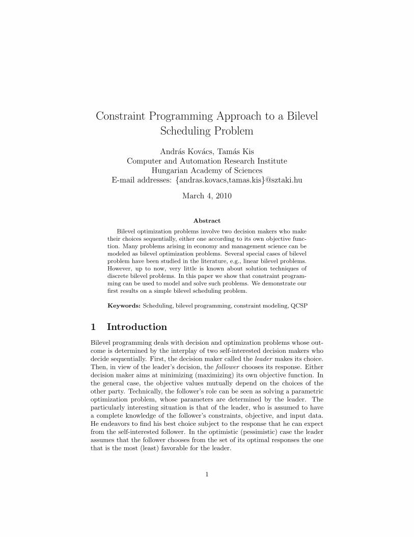
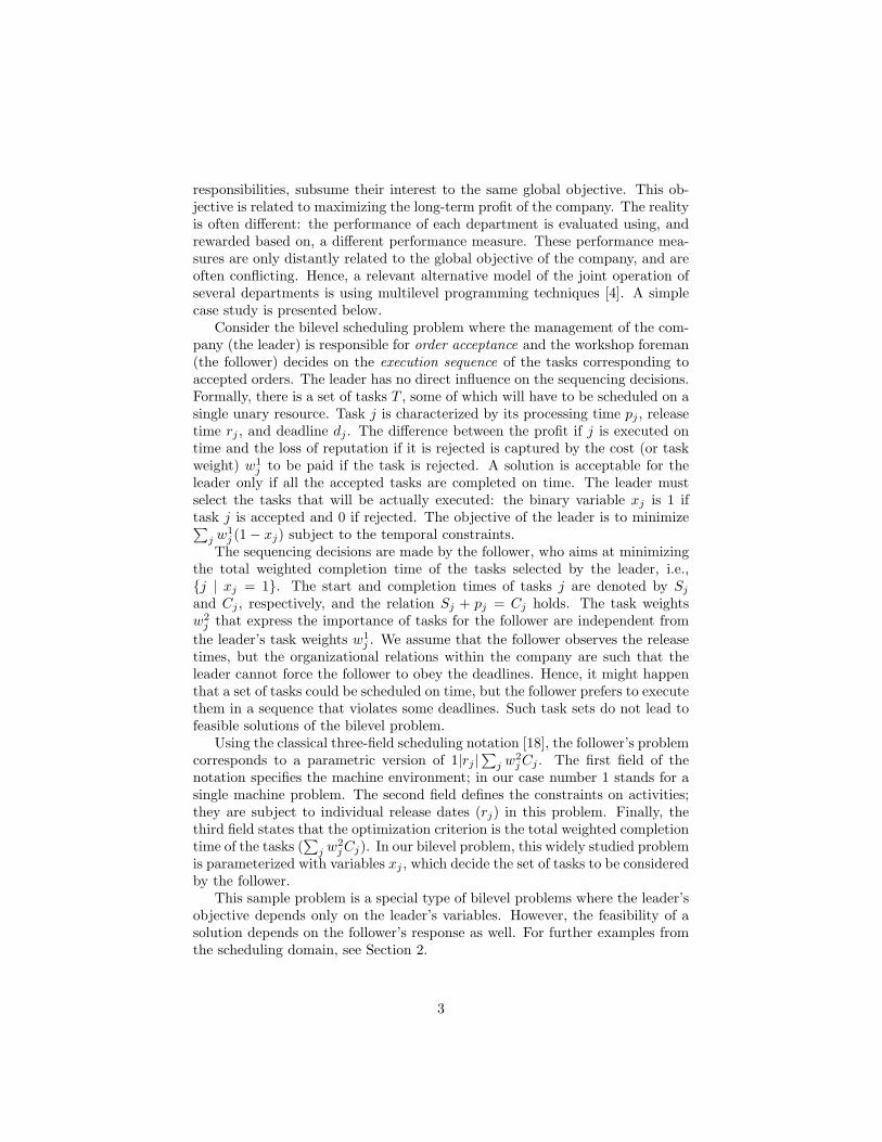
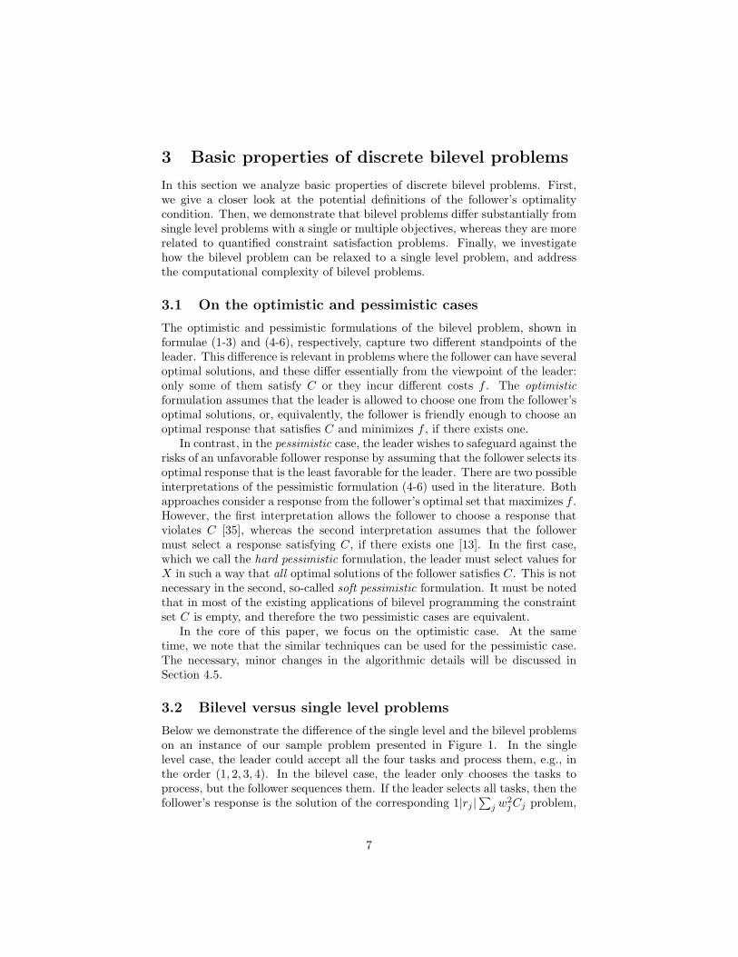
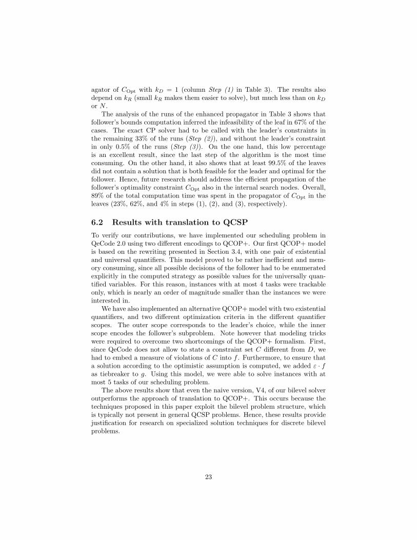
Below we demonstrate the difference of the single level and the bilevel problemson an instance of our sample problem presented in Figure 1. In the singlelevel case, the leader could accept all the four tasks and process them, e.g., inthe order (1, 2, 3, 4). In the bilevel case, the leader only chooses the tasks toprocess, but the follower sequences them. If the leader selects all tasks, then thefollower’s response is the solution of the corresponding 1|rj |

∑j w

2jCj problem,

7

i.e., the sequence (4, 3, 2, 1). This solution is infeasible, because task 1 violatesits deadline. In fact, the optimal bilevel solution is selecting the tasks {1, 2, 3},and processing them in the order (1, 3, 2), which respects all deadlines. Aninteresting, seemingly paradoxical situation is that the strictly smaller set oftasks {1, 2} cannot be scheduled, because the follower’s response, (2, 1), violatesthe deadline of task 1. This also warns us that inference methods that work forthe single level case might not generalize to the bilevel problem.

Task j pj rj dj w1j w2

j

1 1 0 1 2 12 2 0 100 2 43 1 1 100 2 204 1 0 100 1 5

2

2 30

13 2

2 40

1

1

3 2

2 40

1

1

4

5

Figure 1: A bilevel problem instance and the follower’s response for variouschoices of the leader. The tasks marked with a thick frame in the schedulesviolate their deadlines.

3.3 Bilevel versus bicriteria approaches

Although both bilevel programming and single level bicriteria approaches seekfor solutions that are attractive w.r.t. two different objective functions, the twoapproaches differ essentially. They model two different situations: bicriteriaoptimization looks for the best compromise in a centralized way, while bileveloptimization follows a simple, hierarchical protocol with two autonomous part-ners, each interested in optimizing its own objective value. Indeed, the optimalsolution of the bilevel problem might not be Pareto optimal for the correspond-ing single level bicriteria problem, and vice versa. Below we illustrate thisphenomenon on our sample problem.

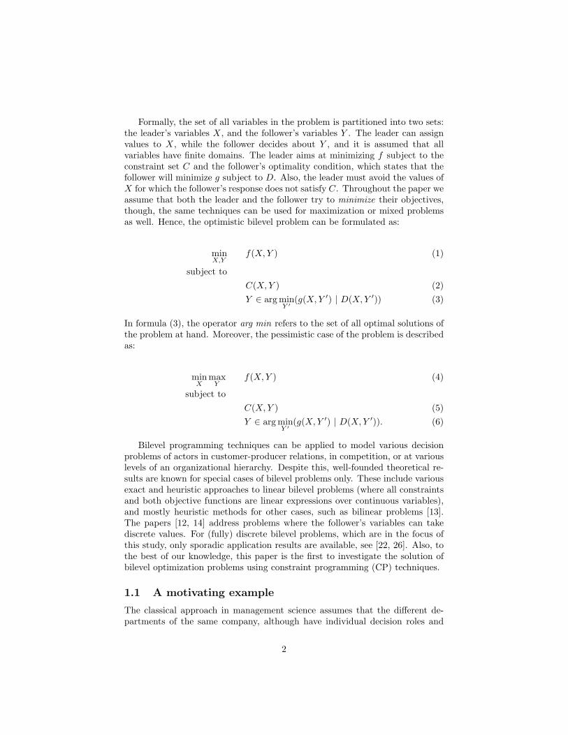
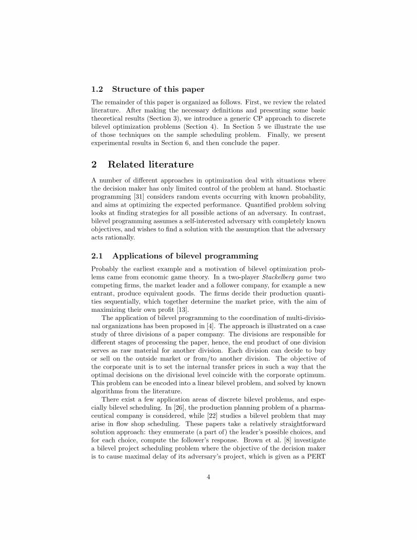
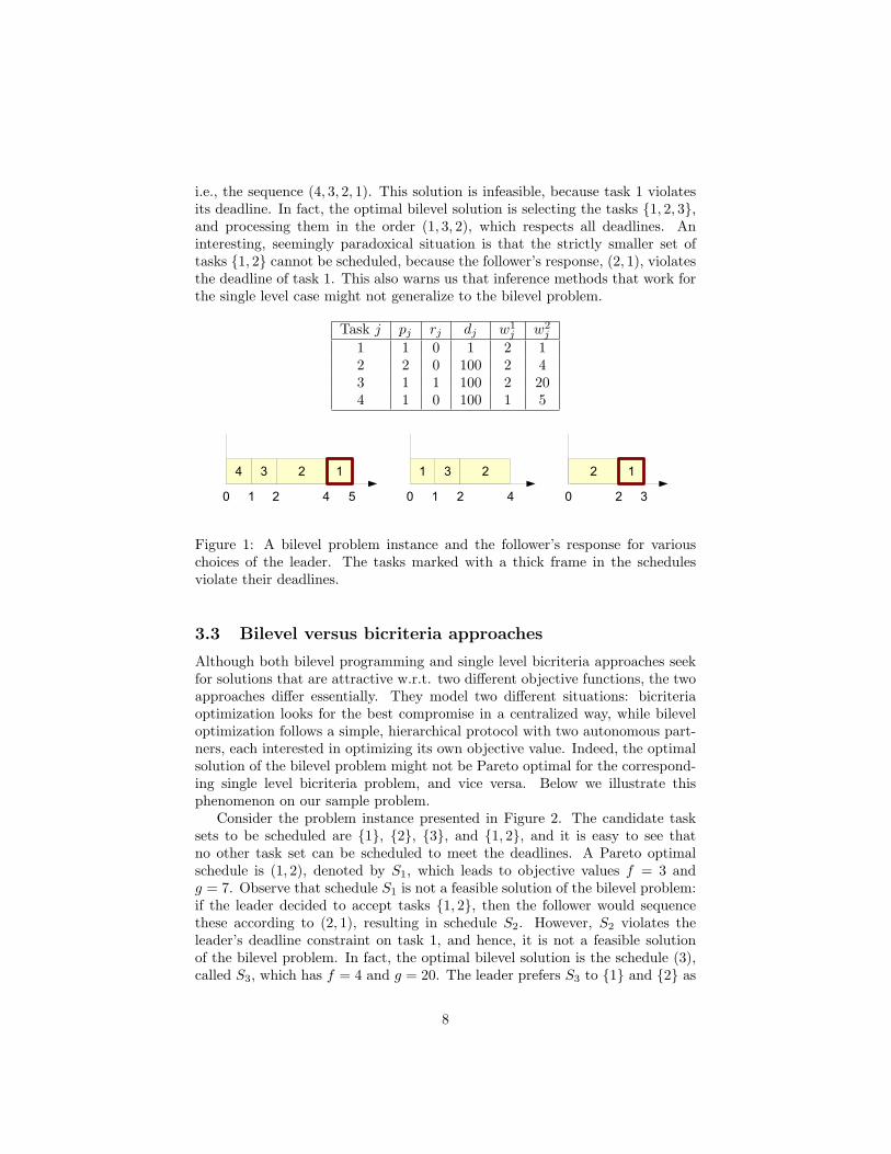
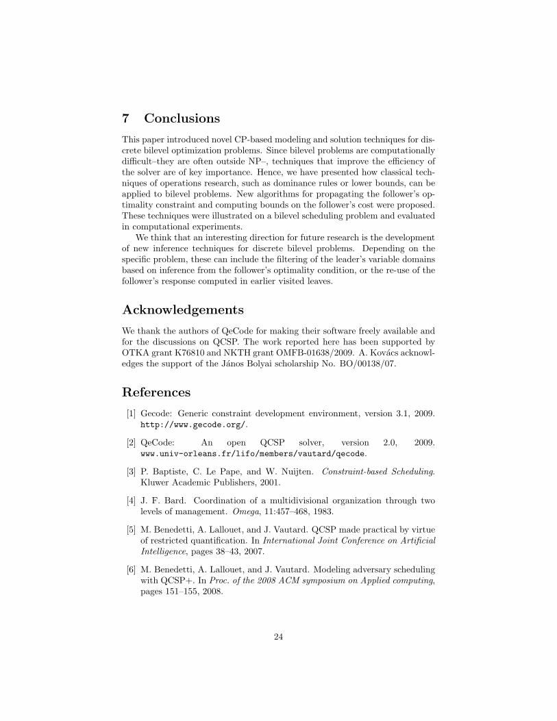
Consider the problem instance presented in Figure 2. The candidate tasksets to be scheduled are {1}, {2}, {3}, and {1, 2}, and it is easy to see thatno other task set can be scheduled to meet the deadlines. A Pareto optimalschedule is (1, 2), denoted by S1, which leads to objective values f = 3 andg = 7. Observe that schedule S1 is not a feasible solution of the bilevel problem:if the leader decided to accept tasks {1, 2}, then the follower would sequencethese according to (2, 1), resulting in schedule S2. However, S2 violates theleader’s deadline constraint on task 1, and hence, it is not a feasible solutionof the bilevel problem. In fact, the optimal bilevel solution is the schedule (3),called S3, which has f = 4 and g = 20. The leader prefers S3 to {1} and {2} as

8

Task j pj rj dj w1j w2

j

1 1 0 1 2 12 1 0 2 2 33 2 0 2 3 10

1 2

S1

3

1 20

S3

S2

2 1

1 20 20

Schedule f g Feasibility OptimalityS1 3 7 Feasible Pareto optimalS2 3 5 Infeasible, task 1 violates deadline -S3 4 20 Feasible Bilevel optimal

Figure 2: Difference of the bilevel and the bicriteria Pareto optimal solutions.The figure presents a problem instance and its three different solutions.

well. Note that S1 Pareto dominates S3, which means that the bilevel optimalsolution is Pareto dominated.

3.4 Bilevel programming versus QCSP

As it has been described above, the main difference between QCSP and bilevelprogramming is that in QCSP, one wishes to find a strategy that covers allpossible actions of the adversary, whereas in bilevel programming we assumethat the follower will act rationally according to its known objectives. Now weshow that bilevel programs can be translated into a QCOP+ with a single pairof quantifiers ∃�∀� and vice versa. We assume that the function symbols f andg and the relation ≤ is available in the constraint language.

First, note that the optimistic bilevel problem corresponds to the QCOP+

minX,Y{f(X,Y ) | C(X,Y ) ∧ D(X,Y ) ∧

∀Y ′[D(X,Y ′)] g(X,Y ) ≤ g(X,Y ′)}.

Here, the first line of the formula describes that 〈X,Y 〉 is a feasible solution,while the second line states that 〈X,Y 〉 is an optimal response of the follower,because all the alternative responses Y ′ would result in a greater or equal valueof g. Furthermore, the hard pessimistic bilevel problem can be rewritten as

9

minX,Y{f(X,Y ) | C(X,Y ) ∧ D(X,Y ) ∧

∀Y ′[D(X,Y ′)] g(X,Y ) ≤ g(X,Y ′)∧∀Y ′′[D(X,Y ′′) ∧ g(X,Y ) = g(X,Y ′′)]

C(X,Y ′′) ∧ f(X,Y ) ≥ f(X,Y ′′)}.

Similarly to the optimistic case, the first and second lines describe that thesolution 〈X,Y 〉 is feasible and optimal for the follower. The third and fourthlines encode the hard pessimistic assumption, i.e., that all the optimal responsesof the follower Y ′′ must satisfy C and result in a value of f not worse thanf(X,Y ). Note that the QCOP+ equivalent of a soft pessimistic bilevel programcan be derived from the above formula by omitting C(X,Y ′′) from the last line.

Although translation to QCOP+ is a theoretically sound approach to solv-ing bilevel problems, it can be rather inefficient. The main deficiency of theapproach is that the computed strategy must cover all possible decisions of thefollower explicitly. To verify these claims, we have implemented our sampleproblem in QeCode. Experimental results are presented in Section 6.

3.5 The single level relaxation

Various components of the solution algorithms for bilevel problems rely on wellunderstood techniques for single level problems. Therefore, it seems naturalto look for relations between bilevel and single level problems. The simplestway of reduction is to let the leader decide on every variable, and completelydisregard the existence of the follower. The resulting problem will be called thesingle level relaxation of the bilevel problem, and its solution value is obviouslya lower bound on the bilevel solution cost:

Definition 1 The single level relaxation of a bilevel program is, using the setof all variables X ′ = (X,Y ), the problem min{f(X ′) | C(X ′) ∧D(X ′)}.

3.6 Computational complexity

Bilevel problems are complex optimization problems, they often belong to ahigher complexity class than their corresponding single level relaxations. Forexample, linear bilevel problems (where both the single level relaxation and thefollower’s subproblem is a linear program) are known to be NP-complete [13].Here, we focus on the complexity of decision versions of discrete bilevel problems,especially in the case where the (decision version of the) single level relaxationis NP-hard. It is easy to observe that a bilevel problem is–except for degeneratecases–at least as complex as its single level relaxation, hence, NP-hard. On theother hand, discrete bilevel problems are in PSPACE, because all instantiationsof the variables can be enumerated and evaluated in polynomial space usinga recursive algorithm, similarly to the algorithm defined for solving quantifiedboolean formulae in [15].

10

Now, a discrete bilevel program may or may not belong to NP. It is easyto define discrete bilevel problems with an NP-compete follower’s subproblemthat are outside NP. Consider an unconventional, but valid bilevel schedul-ing problem where all variables belong to the follower. Both the leader andthe follower aim at sequencing the set of tasks on a single machine subjectto release times rj and strict deadlines dj . However, the leader would be inter-ested in minimizing

∑Cj , whereas the follower minimizes the weighted earliness

penalty∑wj(dj−Cj). This problem is NP-hard, because with follower weights

wj ≡ 0, all solutions are equivalent for the follower, and hence, the optimisticbilevel problem corresponds to the classical 1|rj , dj |

∑Cj problem, which is

NP-hard [25]. On the other hand, it is also co-NP-hard, because with followerweights wj ≡ 1 the two criteria are the negatives of each other. Hence, verifyingthe feasibility of a bilevel solution is equivalent to proving that no better solu-tion exists for the follower’s NP-hard subproblem, 1|rj , dj |

∑wj(dj−Cj). Since

the bilevel problem is both NP-hard and co-NP-hard, it is outside NP (unlessP=NP).

The above complexity results indicate that no direct encoding of discretebilevel problems into CP or MIP can be expected. For the case of our mainsample problem, we were not able to prove that it is outside NP, but we conjec-ture that it is, since no trivial certificate seems to exist for a positive answer.

4 Modeling and solving bilevel problems by CP

In this section we first present a generic approach to solving discrete bileveloptimization problems by CP. Then, we introduce several algorithmic techniquesto improve the efficiency of the solver. Each of the subsections has a counterpartin the Section 5, where the use of the given technique is illustrated on the samplescheduling problem. Unless stated otherwise, we consider the optimistic bilevelproblem.

We use the notation Dom(X) for the current domain of a CP variable Z.Furthermore, the minimum and maximum values in Dom(X) will be denotedby Z and Z, respectively.

4.1 The basic constraint model

Given the discrete optimistic bilevel problem as described in formulae (1-3), letus define an equivalent constraint program that encodes the problem from theleader’s point of view. We also call it the master problem. The decision variablesare both X and Y . They are subject to constraints C and COpt, where C isthe set of the leader’s constraints, and COpt describes the follower’s optimalitycondition:

minX,Y{ f(X,Y ) | C ∧ COpt},

whereCOpt : Y ∈ arg min

Y ′{g(X,Y ′) | D(X,Y ′)}.

11

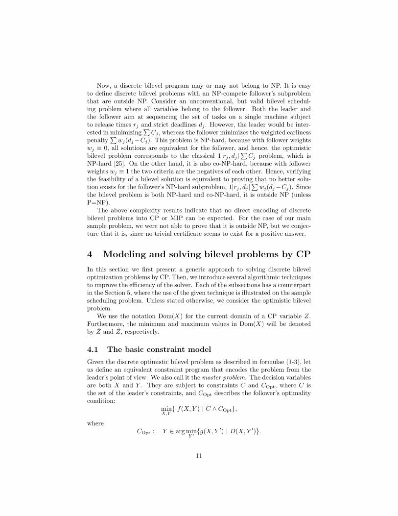
The optimization problem contained in COpt is called the follower’s subprob-lem. We assume that C is a set of classical constraints over finite-domain vari-ables, which have appropriate propagation algorithms defined in the literature.In contrast, in the generic case, constraint COpt contains the parametric versionof an NP-hard discrete optimization problem. Hence, there is little hope thatalgorithms readily available in the literature can be applied to propagate it, orgeneralized arc-consistency can be achieved efficiently. Therefore, we propose tosettle for a generate-and-test approach for propagating COpt, i.e., to propagateonly when all of the leader’s variables X become bound. The pseudo-code of thepropagation algorithm is presented in Figure 3. The algorithm first determinesthe follower’s minimum cost, g∗ (line 3), or returns the symbol ’no solution’ ifno feasible solution exists. Then, it computes the follower’s response accordingto the optimistic assumptions, Y + (line 6). Both of these steps require solvingthe follower’s subproblem with known parameters X. Exact solution approach,e.g., CP search must be used, since the bilevel problem formulation requiresfinding exact optimum. When solving the follower’s subproblem in lines 3 and6, the domains of Y in the master problem must be ignored, since those do-mains are corrupted by the propagators of C, i.e., constraints that the followerdisregards.

PROCEDURE Propagate C Opt()

1 IF X is not bound

2 RETURN

3 LET g∗ := minY ′{g(X, Y ′) | D(X, Y ′)}4 IF g∗ = ’no solution’5 Fail

6 LET Y + := arg minY ′{f(X, Y ′) | g(X, Y ′) = g∗ ∧ C(X, Y ′) ∧D(X, Y ′)}7 IF Y + = ’no solution’8 Fail

9 Instantiate Y ← Y +

Figure 3: Algorithm for propagating constraint COpt.

Regarding search techniques for the master problem, we propose to performany kind of search, exact or non-exact, in the space of the instantiations of theleader’s variables. It is not necessary to consider the follower’s variables, sincevalues will be assigned to them by constraint COpt.

4.2 Lifting the follower’s constraints and dominance rulesinto the master problem

The above basic CP formulation can be strengthened by adding redundant con-straints that propagate even when a part of the variables X is not bound. First,observe that the constraint set D can be added to the basic model, because it

12

reduces the search space to values of X that have at least one feasible followerresponse. Furthermore, assume that there are weak dominance rules known forthe follower’s sub-problem, i.e., properties that all optimal solutions of the sub-problem must satisfy. Then, the conjunct of these rules can be encoded into aconstraint CDom, and added to the CP model as a redundant constraint. Hence,the following CP model is a sound representation of the bilevel problem, and itleads to stronger propagation than the basic model:

minX,Y{ f(X,Y ) | C ∧D ∧ COpt ∧ CDom}.

4.3 Bounds on the follower’s cost

Below we present a novel technique that prunes the search tree based on thedifference of the constraint sets that the leader and the follower must satisfy.We will characterize the values that g can take in solutions that are feasiblefor the leader, as well as the values that g can take in optimal responses of thefollower. Clearly, if the two ranges do not overlap, then there is no feasiblebilevel solution in the current branch of the search tree.

Let UB denote the value of the best known solution, and let us characterizethe current branch of the search tree by the domain of X, denoted by Dom(X).Any feasible improving solution of the master problem must obey C, D, andf < UB. Hence, a valid lower bound gLmin on the values g in the solutions thatare acceptable for the leader in the current branch is:

gLmin = minX′∈Dom(X)

minY{g(X ′, Y ) |

C(X ′, Y ) ∧ D(X ′, Y ) ∧ f(X ′, Y ) < UB}.

On the other hand, for any fixed leader’s choice in this branch, the followerwill return a response that minimizes g subject to D. By taking the maximumof these minimum values, we get an upper bound gFmax on g in the solutionsthat are acceptable for the follower in the current branch:

gFmax = maxX′∈Dom(X)

minY{g(X ′, Y ) | D(X ′, Y )}.

Note that the constraints in the definition of gFmax are a subset of theconstraints for gLmin, and therefore gFmax < gLmin can occur. This meansthat no solution in the current branch of the search tree is both feasible for theleader and optimal for the follower. At the same time gFmax ≥ gLmin is alsopossible, since gFmax is a maximin, whereas gLmin is a minimum.

Lemma 1 If gFmax < gLmin, then the current search branch contains no fea-sible improving bilevel solution, and therefore it can be fathomed.

13

In general, it is difficult to compute the exact values of gFmax and gLmin. In-stead, an upper estimate of gFmax, denote by gFmax can be used, and similarly,a lower estimate of gLmin, denoted by gLmin can be applied.

Finally, note that the application of the above bounds makes sense in theleaves of the search tree as well, since they may prove the infeasibility of theleaf faster than solving the follower’s subproblem in an exact way.

4.4 Lower bounds on the leader’s cost

In theory, it is straightforward to apply the classical lower bounding techniqueof operations research to bilevel problems: let f be a lower bound and f anupper bound, typically the value of the best known solution. Now, if f ≥ fthen the current branch of the search tree does not contain a feasible improvingsolution. In practice, the effective use of this technique is challenging, becausegood lower bounds for bilevel problems are rarely available from the literature.A possible approach is using the single level relaxation, whose solution imposesa lower bound on the bilevel problem. If the single level relaxation is stillintractable, then it can be relaxed further. We note that the value of the singlelevel relaxation is often far from the optimal solution of the bilevel problem.

4.5 Extension to the pessimistic case

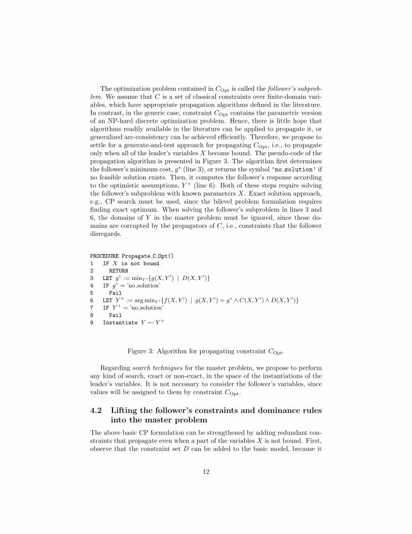
The models and algorithms for the optimistic case can be extended easily to thepessimistic case. The extension requires modifying the propagator of COpt. Inthe soft pessimistic case, the function min in line 6 of Figure 3 must be replacedwith max as follows:

6 LET Y + := arg maxY ′{f(X, Y ′) | g(X, Y ′) = g∗ ∧ C(X, Y ′) ∧D(X, Y ′)}

In the hard pessimistic case, in addition to the above change, the following linesmust be inserted after line 5 (outside the IF-THEN branch of lines 4-5) to ensurethat the follower does not have an optimal solution that violates C:

5a IF there exists an Y ′ such that {g(X, Y ′) = g∗ ∧ C(X, Y ′) ∧D(X, Y ′)}5b Fail

In line 5a, the expression C stands for the negation of C, i.e., C = ∨c∈C¬c.Hence, C corresponds to a reified constraint. We note that the use of reifiedconstraints in C makes the CP approach substantially less efficient for hardpessimistic problems, and may limit the applicable constraints depending onthe solver used. The enhancements presented in Sections 4.2-4.4 can be appliedwithout any change.

14

5 Modeling and solving the scheduling problem

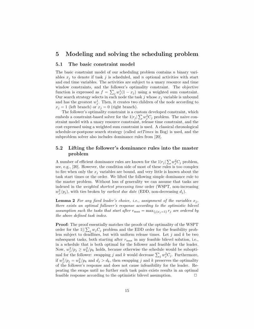
5.1 The basic constraint model

The basic constraint model of our scheduling problem contains n binary vari-ables xj to denote if task j is scheduled, and n optional activities with startand end time variables. The activities are subject to a unary resource and timewindow constraints, and the follower’s optimality constraint. The objectivefunction is expressed as f =

∑j w

1j (1 − xj) using a weighted sum constraint.

Our search strategy selects in each node the task j whose xj variable is unboundand has the greatest w1

j . Then, it creates two children of the node according toxj = 1 (left branch) or xj = 0 (right branch).

The follower’s optimality constraint is a custom developed constraint, whichembeds a constraint-based solver for the 1|rj |

∑w2

jCj problem. The naive con-straint model with a unary resource constraint, release time constraint, and thecost expressed using a weighted sum constraint is used. A classical chronologicalschedule-or-postpone search strategy (called setTimes in Ilog) is used, and thesubproblem solver also includes dominance rules from [20].

5.2 Lifting the follower’s dominance rules into the masterproblem

A number of efficient dominance rules are known for the 1|rj |∑w2

jCj problem,see, e.g., [20]. However, the condition side of most of these rules is too complexto fire when only the xj variables are bound, and very little is known about thetask start times or the order. We lifted the following simple dominance rule tothe master problem. Without loss of generality we can assume that tasks areindexed in the weighted shortest processing time order (WSPT, non-increasingw2

j/pj), with ties broken by earliest due date (EDD, non-decreasing dj).

Lemma 2 For any fixed leader’s choice, i.e., assignment of the variables xj,there exists an optimal follower’s response according to the optimistic bilevelassumption such the tasks that start after rmax = max{j|xj=1} rj are ordered bythe above defined task index.

Proof: The proof essentially matches the proofs of the optimality of the WSPTorder for the 1||

∑j wjCj problem and the EDD order for the feasibility prob-

lem subject to deadlines, but with uniform release times. Let j and k be twosubsequent tasks, both starting after rmax in any feasible bilevel solution, i.e.,in a schedule that is both optimal for the follower and feasible for the leader.Now, w2

j/pj ≥ w2k/pk holds, because otherwise the schedule would be subopti-

mal for the follower: swapping j and k would decrease∑

j w2jCj . Furthermore,

if w2j/pj = w2

k/pk and dj > dk, then swapping j and k preserves the optimalityof the follower’s response and does not cause infeasibility for the leader. Re-peating the swaps until no further such task pairs exists results in an optimalfeasible response according to the optimistic bilevel assumption. 2

15

PROCEDURE Propagate Dominance()

1 LET rmax := max{j|1∈Dom(xj)} rj

2 s := 03 FORALL j ∈ {1, ..., n} IN INCREASING ORDER

4 IF xj is bound to 1 AND Sj ≥ rmax

5 Update S′j := max(Sj , s)6 s := S′j + pj

7 ELSE IF s > Sj

8 Update S′j := max(rmax − 1, rj)9 e :=∞10 FORALL j ∈ {1, ..., n} IN DECREASING ORDER

11 IF xj is bound to 1 AND Sj ≥ rmax

12 Update C′j := min(Cj , e)

13 e := C′j − pj

14 ELSE IF e < Cj

15 Update S′j := max(rmax − 1, rj)

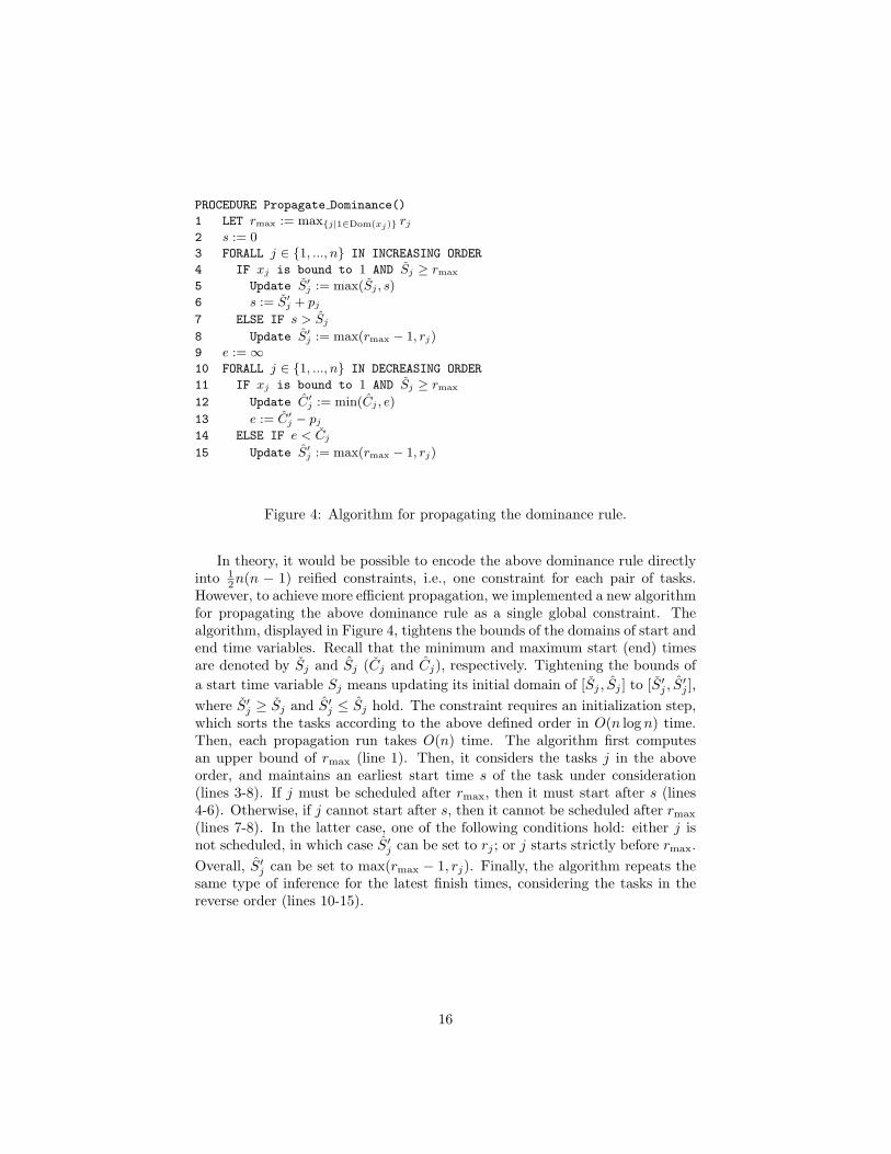
Figure 4: Algorithm for propagating the dominance rule.

In theory, it would be possible to encode the above dominance rule directlyinto 1

2n(n − 1) reified constraints, i.e., one constraint for each pair of tasks.However, to achieve more efficient propagation, we implemented a new algorithmfor propagating the above dominance rule as a single global constraint. Thealgorithm, displayed in Figure 4, tightens the bounds of the domains of start andend time variables. Recall that the minimum and maximum start (end) timesare denoted by Sj and Sj (Cj and Cj), respectively. Tightening the bounds ofa start time variable Sj means updating its initial domain of [Sj , Sj ] to [S′j , S

′j ],

where S′j ≥ Sj and S′j ≤ Sj hold. The constraint requires an initialization step,which sorts the tasks according to the above defined order in O(n log n) time.Then, each propagation run takes O(n) time. The algorithm first computesan upper bound of rmax (line 1). Then, it considers the tasks j in the aboveorder, and maintains an earliest start time s of the task under consideration(lines 3-8). If j must be scheduled after rmax, then it must start after s (lines4-6). Otherwise, if j cannot start after s, then it cannot be scheduled after rmax

(lines 7-8). In the latter case, one of the following conditions hold: either j isnot scheduled, in which case S′j can be set to rj ; or j starts strictly before rmax.Overall, S′j can be set to max(rmax − 1, rj). Finally, the algorithm repeats thesame type of inference for the latest finish times, considering the tasks in thereverse order (lines 10-15).

16

5.3 Bounds on the follower’s cost

5.3.1 The upper bound

Our follower’s subproblem is 1|rj |∑w2

jCj . Let g(T1) denote the follower’s min-imal cost when the leader accepts the task set T1. It is obvious that if T1 ⊆ T2

then g(T1) ≤ g(T2). Therefore, the cost of any heuristic solution to the fol-lower’s problem with task set Tmax = {j | 1 ∈ Dom(xj)} can be used as gFmax.In our solver, we have implemented the constructive heuristic called CPRTWTwith the makeBetter improvement step after the insertion of each task to theschedule, originally introduced in [21].

5.3.2 The lower bound

Computing gLmin requires obtaining a lower bound on a∑w2

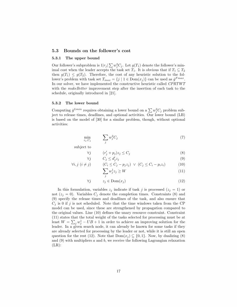
jCj problem sub-ject to release times, deadlines, and optional activities. Our lower bound (LB)is based on the model of [30] for a similar problem, though, without optionalactivities:

minzj ,Cj

∑j

w2jCj (7)

subject to∀j (r′j + pj)zj ≤ Cj (8)∀j Cj ≤ d′jzj (9)

∀i, j (i 6= j) (Ci ≤ Cj − pjzj) ∨ (Cj ≤ Ci − pizi) (10)∑j

w1j zj ≥W (11)

∀j zj ∈ Dom(xj) (12)

In this formulation, variables zj indicate if task j is processed (zj = 1) ornot (zj = 0). Variables Cj denote the completion times. Constraints (8) and(9) specify the release times and deadlines of the task, and also ensure thatCj is 0 if j is not scheduled. Note that the time windows taken from the CPmodel can be used, since these are strengthened by propagation compared tothe original values. Line (10) defines the unary resource constraint. Constraint(11) states that the total weight of the tasks selected for processing must be atleast W =

∑j w

1j − UB + 1 in order to achieve an improving solution for the

leader. In a given search node, it can already be known for some tasks if theyare already selected for processing by the leader or not, while it is still an openquestion for the rest (12). Note that Dom(xj) ⊆ {0, 1}. Now, by dualizing (8)and (9) with multipliers a and b, we receive the following Lagrangian relaxation(LR):

17

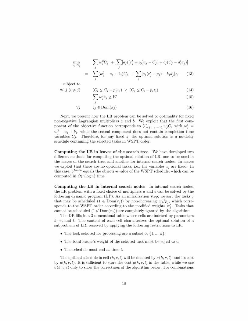
minzj ,Cj

∑j

w2jCj +

∑j

[aj((r′j + pj)zj − Cj) + bj(Cj − d′jzj)]

=∑

j

(w2j − aj + bj)Cj +

∑j

[aj(r′j + pj)− bjd′j ]zj (13)

subject to∀i, j (i 6= j) (Ci ≤ Cj − pjzj) ∨ (Cj ≤ Ci − pizi) (14)∑

j

w1j zj ≥W (15)

∀j zj ∈ Dom(xj) (16)

Next, we present how the LR problem can be solved to optimality for fixednon-negative Lagrangian multipliers a and b. We exploit that the first com-ponent of the objective function corresponds to

∑{j | zj=1} w

′jCj with w′j =

w2j − aj + bj , while the second component does not contain completion time

variables Cj . Therefore, for any fixed z, the optimal solution is a no-delayschedule containing the selected tasks in WSPT order.

Computing the LB in leaves of the search tree We have developed twodifferent methods for computing the optimal solution of LR: one to be used inthe leaves of the search tree, and another for internal search nodes. In leaveswe exploit that there are no optional tasks, i.e., the variables zj are fixed. Inthis case, gLmin equals the objective value of the WSPT schedule, which can becomputed in O(n log n) time.

Computing the LB in internal search nodes In internal search nodes,the LR problem with a fixed choice of multipliers a and b can be solved by thefollowing dynamic program (DP). As an initialization step, we sort the tasks jthat may be scheduled (1 ∈ Dom(xj)) by non-increasing w′j/pj , which corre-sponds to the WSPT order according to the modified weights w′j . Tasks thatcannot be scheduled (1 6∈ Dom(xj)) are completely ignored by the algorithm.

The DP fills in a 3 dimensional table whose cells are indexed by parametersk, v, and t. The content of each cell characterizes the optimal solution of asubproblem of LR, received by applying the following restrictions to LR:

• The task selected for processing are a subset of {1, ..., k};

• The total leader’s weight of the selected task must be equal to v;

• The schedule must end at time t.

The optimal schedule in cell (k, v, t) will be denoted by σ(k, v, t), and its costby u(k, v, t). It is sufficient to store the cost u(k, v, t) in the table, while we useσ(k, v, t) only to show the correctness of the algorithm below. For combinations

18

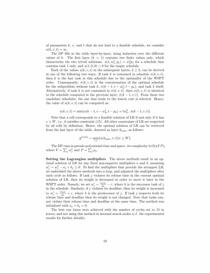
of parameters k, v, and t that do not lead to a feasible schedule, we consideru(k, v, t) =∞.

The DP fills in the table layer-by-layer, using induction over the differentvalues of k. The first layer (k = 1) contains two finite values only, whichcharacterize the two trivial solutions: u(1, w1

1, p1) = w21p1 for a schedule that

contains task 1 only, and u(1, 0, 0) = 0 for the empty schedule.Each of the values u(k, v, t) in the subsequent layers, k ≥ 2, can be derived

in one of the following two ways. If task k is contained in schedule σ(k, v, t),then k is the last task in this schedule due to the optimality of the WSPTorder. Consequently, σ(k, v, t) is the concatenation of the optimal schedulefor the subproblem without task k, σ(k − 1, v − w1

k, t − pk), and task k itself.Alternatively, if task k is not contained in σ(k, v, t), then σ(k, v, t) is identicalto the schedule computed in the previous layer, σ(k − 1, v, t). From these twocandidate schedules, the one that leads to the lowest cost is selected. Hence,the value of u(k, v, t) can be computed as:

u(k, v, t) = min(u(k − 1, v − w1k, t− pk) + tw2

k, u(k − 1, v, t))

Note that a cell corresponds to a feasible solution of LR if and only if it hasv ≥W , i.e., it satisfies constraint (15). All other constraints of LR are respectedby all cells by definition. Hence, the optimal solution of LR can be retrievedfrom the last layer of the table, denoted as layer kmax, as follows:

gLmin = minv,t{u(kmax, v, t)|v ≥W}

The DP runs in pseudo-polynomial time and space: its complexity isO(nV P ),where V =

∑j w

1j and P =

∑j pj .

Setting the Lagrangian multipliers The above methods result in an op-timal solution of LR for any fixed non-negative multipliers a and b, assumingw′j = w2

j − aj + bj ≥ 0. To find the multipliers that provide the strongest LB,we embedded the above methods into a loop, and adjusted the multipliers aftereach cycle as follows. If task j violates its release time in the current optimalsolution of LR, then its weight is decreased in order to move it later in theWSPT order. Namely, we set w′j = w′

kpj

pk− ε, where k is the successor task of j

in the schedule. Similarly, if j violates its deadline, then its weight is increasedto w′j = w′

kpj

pk+ ε, where k is the predecessor of j. If task j respects both its

release time and deadline then its weight is not changed. Note that tasks can-not violate their release time and deadline at the same time. The method wasinitialized with aj = bj = 0.

The best run times were achieved with the number of cycles set to 15 inleaves, and not using this method in internal search nodes (c.f. the experimentalresults for further details).

19

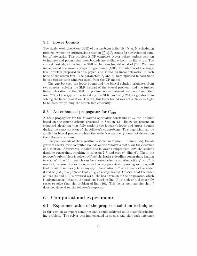
5.4 Lower bounds

The single level relaxation (SLR) of our problem is the 1|rj |∑w1

jUj schedulingproblem, where the optimization criterion

∑w1

jUj stands for the weighted num-ber of late tasks. This problem is NP-complete. Nevertheless, various solutiontechniques and polynomial lower bounds are available from the literature. Thecurrent best algorithm for the SLR is the branch-and-bound of [28]. We haveimplemented the mixed-integer programming (MIP) formulation of the singlelevel problem proposed in this paper, and solved its linear relaxation in eachnode of the search tree. The parameters rj and dj were updated in each nodeby the tighter time windows taken from the CP model.

The gap between the lower bound and the bilevel solution originates fromtwo sources: solving the SLR instead of the bilevel problem, and the furtherlinear relaxation of the SLR. In preliminary experiment we have found thatover 75% of the gap is due to taking the SLR, and only 25% originates fromsolving the linear relaxation. Overall, this lower bound was not sufficiently tightto be used for pruning the search tree efficiently.

5.5 An enhanced propagator for COpt

A basic propagator for the follower’s optimality constraint COpt can be builtbased on the generic scheme presented in Section 4.1. Below we present anenhanced algorithm that fully exploits the follower’s lower and upper boundsduring the exact solution of the follower’s subproblem. This algorithm can beapplied in bilevel problems where the leader’s objective, f , does not depend onthe follower’s response.

The pseudo-code of the algorithm is shown in Figure 5. In lines (3-5), the al-gorithm checks if the computed bounds on the follower’s cost allow the existenceof a solution. Afterwards, it solves the follower’s subproblem with the leader’sdeadline constraints, resulting in solution Y + and cost g+ (line 6). Then, thefollower’s subproblem is solved without the leader’s deadline constraints, leadingto cost g∗ (line 10). Search can be aborted when a solution with g∗ < g+ isreached, because this solution, as well as any potential improving solution, willlead to failure in lines (11-12) anyway. The solution Y + is optimal for the leaderif and only if g+ = g∗ (note that g+ ≥ g∗ always holds). Observe that the orderof lines (6) and (10) is reversed w.r.t. the basic version of the propagator, whichis advantageous because the problem faced in line (6) is tighter and generallyeasier-to-solve than the problem of line (10). This latter step exploits that fdoes not depend on the follower’s response.

6 Computational experiments

6.1 Experimentation of the proposed solution techniques

In this section we report computational results achieved on the sample schedul-ing problem. The solver was implemented in such a way that each inference

20

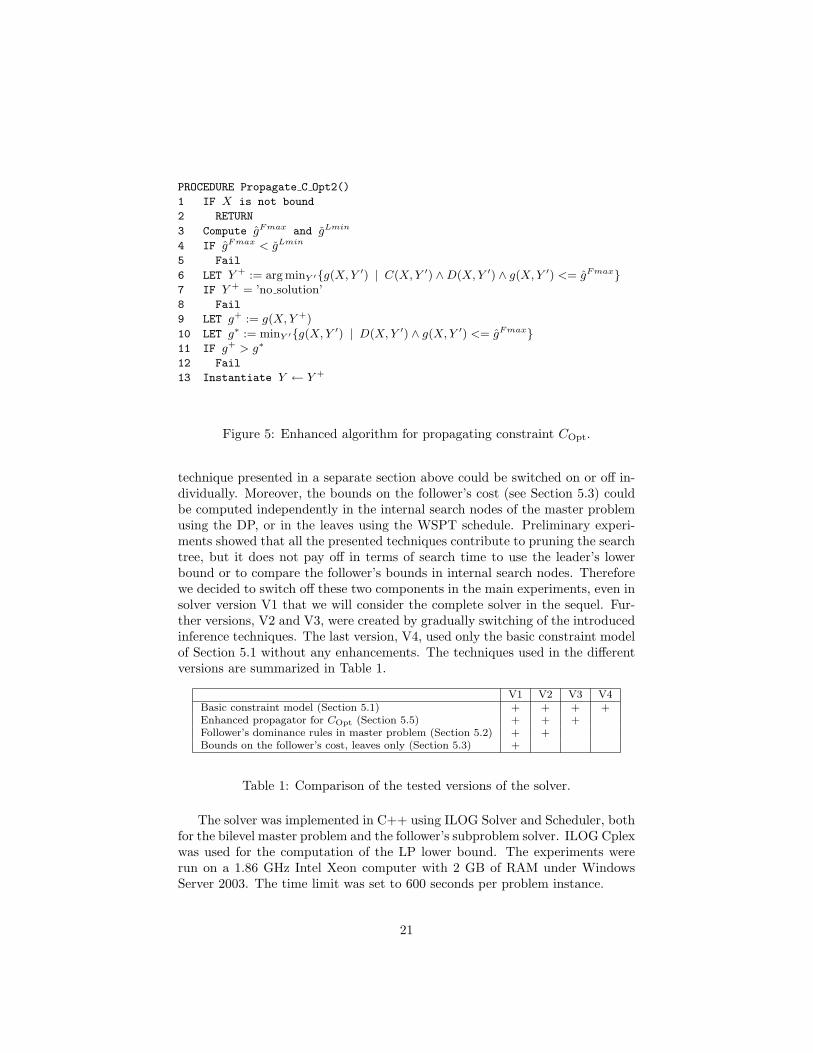
PROCEDURE Propagate C Opt2()

1 IF X is not bound

2 RETURN

3 Compute gFmax and gLmin

4 IF gFmax < gLmin

5 Fail

6 LET Y + := arg minY ′{g(X, Y ′) | C(X, Y ′) ∧D(X, Y ′) ∧ g(X, Y ′) <= gFmax}7 IF Y + = ’no solution’8 Fail

9 LET g+ := g(X, Y +)10 LET g∗ := minY ′{g(X, Y ′) | D(X, Y ′) ∧ g(X, Y ′) <= gFmax}11 IF g+ > g∗

12 Fail

13 Instantiate Y ← Y +

Figure 5: Enhanced algorithm for propagating constraint COpt.

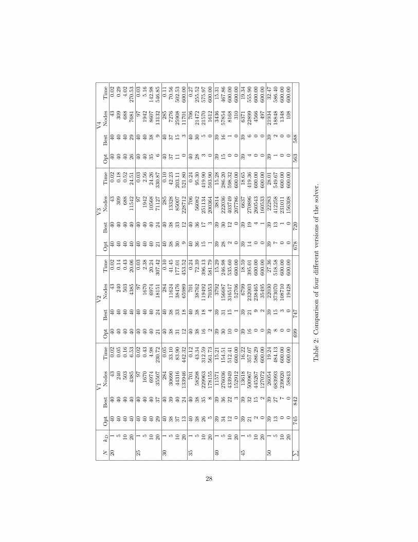
technique presented in a separate section above could be switched on or off in-dividually. Moreover, the bounds on the follower’s cost (see Section 5.3) couldbe computed independently in the internal search nodes of the master problemusing the DP, or in the leaves using the WSPT schedule. Preliminary experi-ments showed that all the presented techniques contribute to pruning the searchtree, but it does not pay off in terms of search time to use the leader’s lowerbound or to compare the follower’s bounds in internal search nodes. Thereforewe decided to switch off these two components in the main experiments, even insolver version V1 that we will consider the complete solver in the sequel. Fur-ther versions, V2 and V3, were created by gradually switching of the introducedinference techniques. The last version, V4, used only the basic constraint modelof Section 5.1 without any enhancements. The techniques used in the differentversions are summarized in Table 1.

V1 V2 V3 V4Basic constraint model (Section 5.1) + + + +Enhanced propagator for COpt (Section 5.5) + + +Follower’s dominance rules in master problem (Section 5.2) + +Bounds on the follower’s cost, leaves only (Section 5.3) +

Table 1: Comparison of the tested versions of the solver.

The solver was implemented in C++ using ILOG Solver and Scheduler, bothfor the bilevel master problem and the follower’s subproblem solver. ILOG Cplexwas used for the computation of the LP lower bound. The experiments wererun on a 1.86 GHz Intel Xeon computer with 2 GB of RAM under WindowsServer 2003. The time limit was set to 600 seconds per problem instance.

21

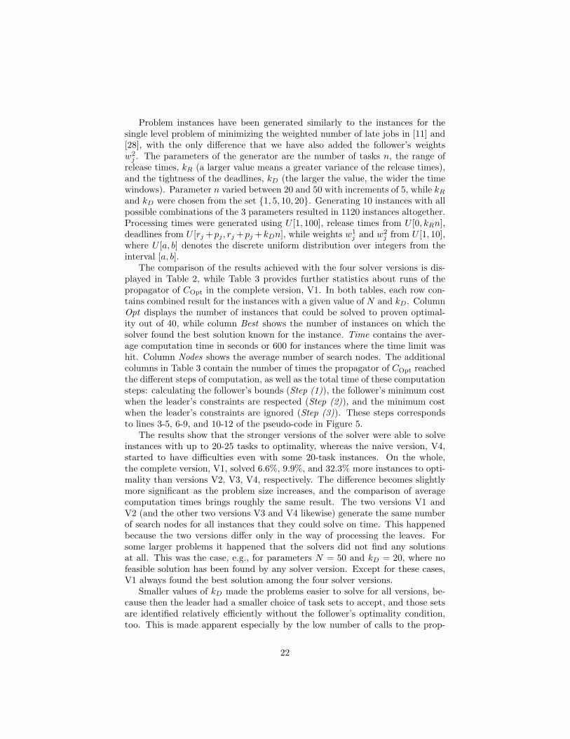
Problem instances have been generated similarly to the instances for thesingle level problem of minimizing the weighted number of late jobs in [11] and[28], with the only difference that we have also added the follower’s weightsw2

j . The parameters of the generator are the number of tasks n, the range ofrelease times, kR (a larger value means a greater variance of the release times),and the tightness of the deadlines, kD (the larger the value, the wider the timewindows). Parameter n varied between 20 and 50 with increments of 5, while kR

and kD were chosen from the set {1, 5, 10, 20}. Generating 10 instances with allpossible combinations of the 3 parameters resulted in 1120 instances altogether.Processing times were generated using U [1, 100], release times from U [0, kRn],deadlines from U [rj +pj , rj +pj +kDn], while weights w1

j and w2j from U [1, 10],

where U [a, b] denotes the discrete uniform distribution over integers from theinterval [a, b].

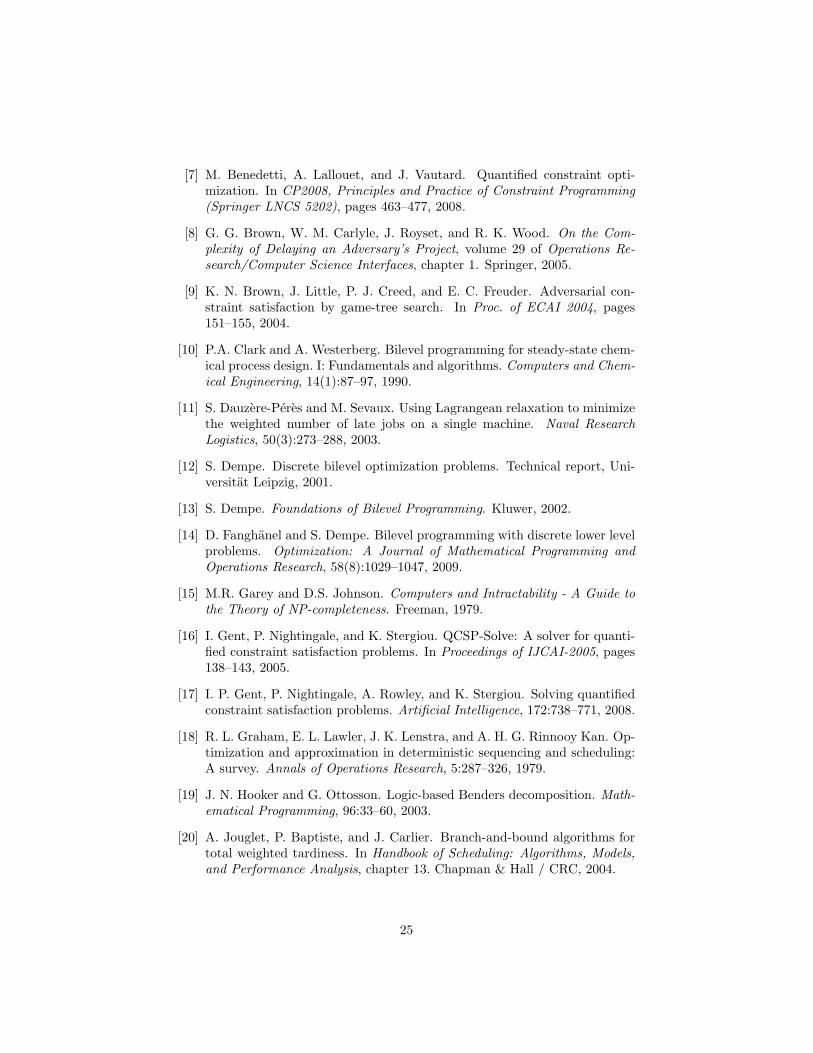
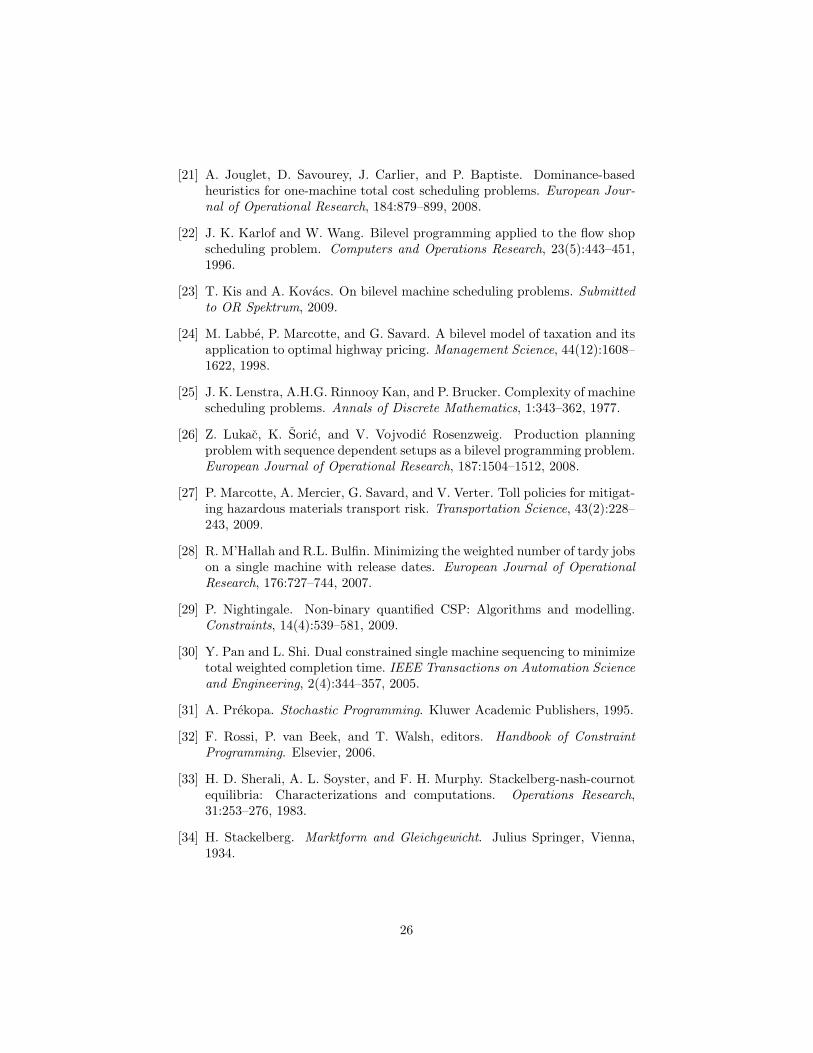
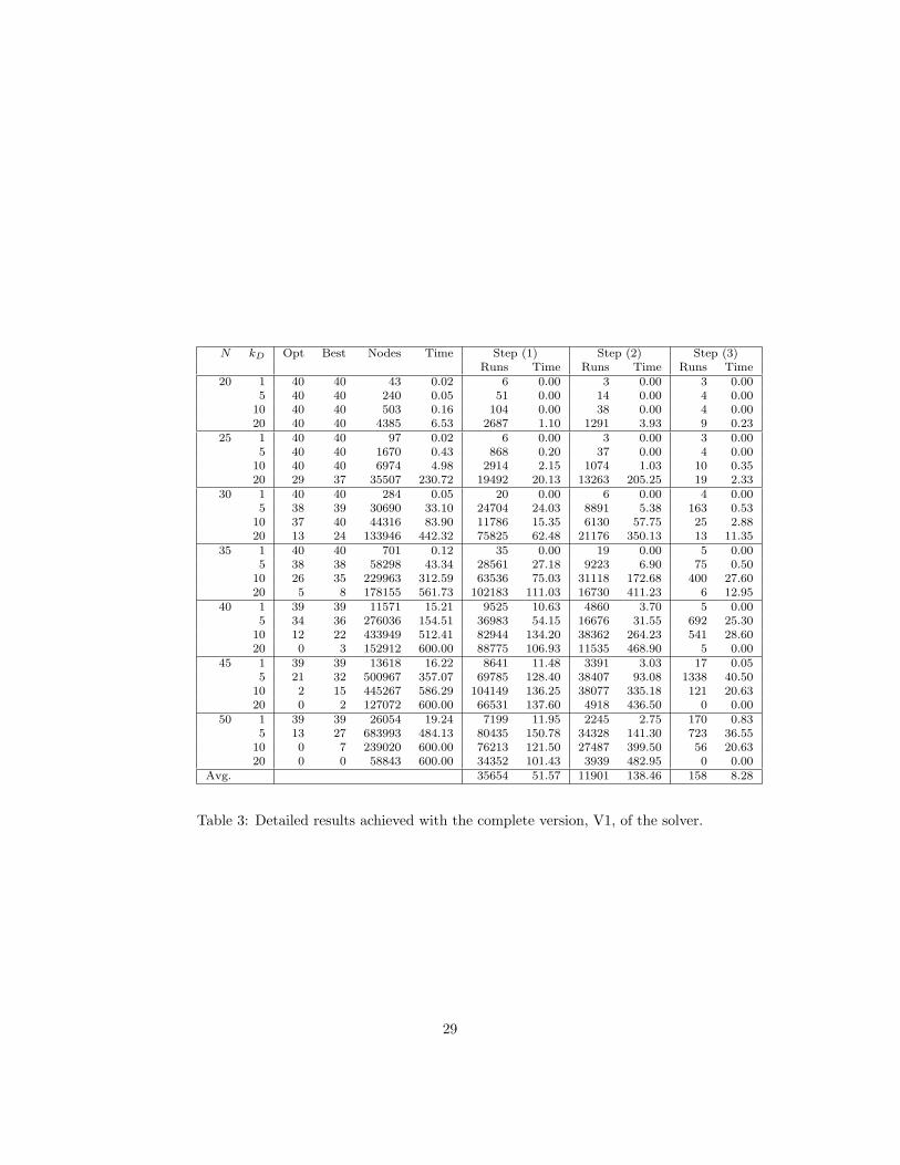
The comparison of the results achieved with the four solver versions is dis-played in Table 2, while Table 3 provides further statistics about runs of thepropagator of COpt in the complete version, V1. In both tables, each row con-tains combined result for the instances with a given value of N and kD. ColumnOpt displays the number of instances that could be solved to proven optimal-ity out of 40, while column Best shows the number of instances on which thesolver found the best solution known for the instance. Time contains the aver-age computation time in seconds or 600 for instances where the time limit washit. Column Nodes shows the average number of search nodes. The additionalcolumns in Table 3 contain the number of times the propagator of COpt reachedthe different steps of computation, as well as the total time of these computationsteps: calculating the follower’s bounds (Step (1)), the follower’s minimum costwhen the leader’s constraints are respected (Step (2)), and the minimum costwhen the leader’s constraints are ignored (Step (3)). These steps correspondsto lines 3-5, 6-9, and 10-12 of the pseudo-code in Figure 5.

The results show that the stronger versions of the solver were able to solveinstances with up to 20-25 tasks to optimality, whereas the naive version, V4,started to have difficulties even with some 20-task instances. On the whole,the complete version, V1, solved 6.6%, 9.9%, and 32.3% more instances to opti-mality than versions V2, V3, V4, respectively. The difference becomes slightlymore significant as the problem size increases, and the comparison of averagecomputation times brings roughly the same result. The two versions V1 andV2 (and the other two versions V3 and V4 likewise) generate the same numberof search nodes for all instances that they could solve on time. This happenedbecause the two versions differ only in the way of processing the leaves. Forsome larger problems it happened that the solvers did not find any solutionsat all. This was the case, e.g., for parameters N = 50 and kD = 20, where nofeasible solution has been found by any solver version. Except for these cases,V1 always found the best solution among the four solver versions.

Smaller values of kD made the problems easier to solve for all versions, be-cause then the leader had a smaller choice of task sets to accept, and those setsare identified relatively efficiently without the follower’s optimality condition,too. This is made apparent especially by the low number of calls to the prop-

22

agator of COpt with kD = 1 (column Step (1) in Table 3). The results alsodepend on kR (small kR makes them easier to solve), but much less than on kD

or N .The analysis of the runs of the enhanced propagator in Table 3 shows that

follower’s bounds computation inferred the infeasibility of the leaf in 67% of thecases. The exact CP solver had to be called with the leader’s constraints inthe remaining 33% of the runs (Step (2)), and without the leader’s constraintin only 0.5% of the runs (Step (3)). On the one hand, this low percentageis an excellent result, since the last step of the algorithm is the most timeconsuming. On the other hand, it also shows that at least 99.5% of the leavesdid not contain a solution that is both feasible for the leader and optimal for thefollower. Hence, future research should address the efficient propagation of thefollower’s optimality constraint COpt also in the internal search nodes. Overall,89% of the total computation time was spent in the propagator of COpt in theleaves (23%, 62%, and 4% in steps (1), (2), and (3), respectively).

6.2 Results with translation to QCSP

To verify our contributions, we have implemented our scheduling problem inQeCode 2.0 using two different encodings to QCOP+. Our first QCOP+ modelis based on the rewriting presented in Section 3.4, with one pair of existentialand universal quantifiers. This model proved to be rather inefficient and mem-ory consuming, since all possible decisions of the follower had to be enumeratedexplicitly in the computed strategy as possible values for the universally quan-tified variables. For this reason, instances with at most 4 tasks were trackableonly, which is nearly an order of magnitude smaller than the instances we wereinterested in.

We have also implemented an alternative QCOP+ model with two existentialquantifiers, and two different optimization criteria in the different quantifierscopes. The outer scope corresponds to the leader’s choice, while the innerscope encodes the follower’s subproblem. Note however that modeling trickswere required to overcome two shortcomings of the QCOP+ formalism. First,since QeCode does not allow to state a constraint set C different from D, wehad to embed a measure of violations of C into f . Furthermore, to ensure thata solution according to the optimistic assumption is computed, we added ε · fas tiebreaker to g. Using this model, we were able to solve instances with atmost 5 tasks of our scheduling problem.

The above results show that even the naive version, V4, of our bilevel solveroutperforms the approach of translation to QCOP+. This occurs because thetechniques proposed in this paper exploit the bilevel problem structure, whichis typically not present in general QCSP problems. Hence, these results providejustification for research on specialized solution techniques for discrete bilevelproblems.

23

7 Conclusions

This paper introduced novel CP-based modeling and solution techniques for dis-crete bilevel optimization problems. Since bilevel problems are computationallydifficult–they are often outside NP–, techniques that improve the efficiency ofthe solver are of key importance. Hence, we have presented how classical tech-niques of operations research, such as dominance rules or lower bounds, can beapplied to bilevel problems. New algorithms for propagating the follower’s op-timality constraint and computing bounds on the follower’s cost were proposed.These techniques were illustrated on a bilevel scheduling problem and evaluatedin computational experiments.

We think that an interesting direction for future research is the developmentof new inference techniques for discrete bilevel problems. Depending on thespecific problem, these can include the filtering of the leader’s variable domainsbased on inference from the follower’s optimality condition, or the re-use of thefollower’s response computed in earlier visited leaves.

Acknowledgements

We thank the authors of QeCode for making their software freely available andfor the discussions on QCSP. The work reported here has been supported byOTKA grant K76810 and NKTH grant OMFB-01638/2009. A. Kovacs acknowl-edges the support of the Janos Bolyai scholarship No. BO/00138/07.

References

[1] Gecode: Generic constraint development environment, version 3.1, 2009.http://www.gecode.org/.

[2] QeCode: An open QCSP solver, version 2.0, 2009.www.univ-orleans.fr/lifo/members/vautard/qecode.

[3] P. Baptiste, C. Le Pape, and W. Nuijten. Constraint-based Scheduling.Kluwer Academic Publishers, 2001.

[4] J. F. Bard. Coordination of a multidivisional organization through twolevels of management. Omega, 11:457–468, 1983.

[5] M. Benedetti, A. Lallouet, and J. Vautard. QCSP made practical by virtueof restricted quantification. In International Joint Conference on ArtificialIntelligence, pages 38–43, 2007.

[6] M. Benedetti, A. Lallouet, and J. Vautard. Modeling adversary schedulingwith QCSP+. In Proc. of the 2008 ACM symposium on Applied computing,pages 151–155, 2008.

24

[7] M. Benedetti, A. Lallouet, and J. Vautard. Quantified constraint opti-mization. In CP2008, Principles and Practice of Constraint Programming(Springer LNCS 5202), pages 463–477, 2008.

[8] G. G. Brown, W. M. Carlyle, J. Royset, and R. K. Wood. On the Com-plexity of Delaying an Adversary’s Project, volume 29 of Operations Re-search/Computer Science Interfaces, chapter 1. Springer, 2005.

[9] K. N. Brown, J. Little, P. J. Creed, and E. C. Freuder. Adversarial con-straint satisfaction by game-tree search. In Proc. of ECAI 2004, pages151–155, 2004.

[10] P.A. Clark and A. Westerberg. Bilevel programming for steady-state chem-ical process design. I: Fundamentals and algorithms. Computers and Chem-ical Engineering, 14(1):87–97, 1990.

[11] S. Dauzere-Peres and M. Sevaux. Using Lagrangean relaxation to minimizethe weighted number of late jobs on a single machine. Naval ResearchLogistics, 50(3):273–288, 2003.

[12] S. Dempe. Discrete bilevel optimization problems. Technical report, Uni-versitat Leipzig, 2001.

[13] S. Dempe. Foundations of Bilevel Programming. Kluwer, 2002.

[14] D. Fanghanel and S. Dempe. Bilevel programming with discrete lower levelproblems. Optimization: A Journal of Mathematical Programming andOperations Research, 58(8):1029–1047, 2009.

[15] M.R. Garey and D.S. Johnson. Computers and Intractability - A Guide tothe Theory of NP-completeness. Freeman, 1979.

[16] I. Gent, P. Nightingale, and K. Stergiou. QCSP-Solve: A solver for quanti-fied constraint satisfaction problems. In Proceedings of IJCAI-2005, pages138–143, 2005.

[17] I. P. Gent, P. Nightingale, A. Rowley, and K. Stergiou. Solving quantifiedconstraint satisfaction problems. Artificial Intelligence, 172:738–771, 2008.

[18] R. L. Graham, E. L. Lawler, J. K. Lenstra, and A. H. G. Rinnooy Kan. Op-timization and approximation in deterministic sequencing and scheduling:A survey. Annals of Operations Research, 5:287–326, 1979.

[19] J. N. Hooker and G. Ottosson. Logic-based Benders decomposition. Math-ematical Programming, 96:33–60, 2003.

[20] A. Jouglet, P. Baptiste, and J. Carlier. Branch-and-bound algorithms fortotal weighted tardiness. In Handbook of Scheduling: Algorithms, Models,and Performance Analysis, chapter 13. Chapman & Hall / CRC, 2004.

25

[21] A. Jouglet, D. Savourey, J. Carlier, and P. Baptiste. Dominance-basedheuristics for one-machine total cost scheduling problems. European Jour-nal of Operational Research, 184:879–899, 2008.

[22] J. K. Karlof and W. Wang. Bilevel programming applied to the flow shopscheduling problem. Computers and Operations Research, 23(5):443–451,1996.

[23] T. Kis and A. Kovacs. On bilevel machine scheduling problems. Submittedto OR Spektrum, 2009.

[24] M. Labbe, P. Marcotte, and G. Savard. A bilevel model of taxation and itsapplication to optimal highway pricing. Management Science, 44(12):1608–1622, 1998.

[25] J. K. Lenstra, A.H.G. Rinnooy Kan, and P. Brucker. Complexity of machinescheduling problems. Annals of Discrete Mathematics, 1:343–362, 1977.

[26] Z. Lukac, K. Soric, and V. Vojvodic Rosenzweig. Production planningproblem with sequence dependent setups as a bilevel programming problem.European Journal of Operational Research, 187:1504–1512, 2008.

[27] P. Marcotte, A. Mercier, G. Savard, and V. Verter. Toll policies for mitigat-ing hazardous materials transport risk. Transportation Science, 43(2):228–243, 2009.

[28] R. M’Hallah and R.L. Bulfin. Minimizing the weighted number of tardy jobson a single machine with release dates. European Journal of OperationalResearch, 176:727–744, 2007.

[29] P. Nightingale. Non-binary quantified CSP: Algorithms and modelling.Constraints, 14(4):539–581, 2009.

[30] Y. Pan and L. Shi. Dual constrained single machine sequencing to minimizetotal weighted completion time. IEEE Transactions on Automation Scienceand Engineering, 2(4):344–357, 2005.

[31] A. Prekopa. Stochastic Programming. Kluwer Academic Publishers, 1995.

[32] F. Rossi, P. van Beek, and T. Walsh, editors. Handbook of ConstraintProgramming. Elsevier, 2006.

[33] H. D. Sherali, A. L. Soyster, and F. H. Murphy. Stackelberg-nash-cournotequilibria: Characterizations and computations. Operations Research,31:253–276, 1983.

[34] H. Stackelberg. Marktform and Gleichgewicht. Julius Springer, Vienna,1934.

26

[35] A. Tsoukalas, W. Wiesemann, and B. Rustem. Global optimisation ofpessimistic bi-level problems. In P. M. Pardalos and T. F. Coleman, editors,Lectures on Global Optimization, pages 215–243. American MathematicalSociety, 2009.

[36] G. Verger and C. Bessiere. Blocksolve: a bottom-up approach for solv-ing quantified CSPs. In CP2006, Principles and Practice of ConstraintProgramming (Springer LNCS 4204), pages 635–649, 2006.

[37] B. von Stengel. Equilibrium computation for two-player games in strate-gic and extensive form. In N. Nisan, T. Roughgarden, E. Tardos, andV.V. Vazirani, editors, Algorithmic Game Theory, chapter 3. CambridgeUniversity Press, 2007.

27

V1

V2

V3

V4

Nk

DO

pt

Bes

tN

odes

Tim

eO

pt

Bes

tN

odes

Tim

eO

pt

Bes

tN

odes

Tim

eO

pt

Bes

tN

odes

Tim

e20

140

40

43

0.0

240

40

43

0.0

240

40

43

0.0

240

40

43

0.0

25

40

40

240

0.0

540

40

240

0.1

440

40

309

0.1

840

40

309

0.2

910

40

40

503

0.1

640

40

503

0.4

340

40

688

0.5

240

40

688

4.0

220

40

40

4385

6.5

340

40

4385

20.0

640

40

11542

24.5

126

29

7681

270.5

325

140

40

97

0.0

240

40

97

0.0

340

40

97

0.0

340

40

97

0.0

35

40

40

1670

0.4

340

40

1670

2.3

840

40

1942

2.5

640

40

1942

5.1

610

40

40

6974

4.9

840

40

6974

20.2

440

40

10568

24.2

635

38

8607

142.9

820

29

37

35507

230.7

221

24

18151

307.4

221

24

71127

330.8

76

913132

546.8

530

140

40

284

0.0

540

40

284

0.1

040

40

285

0.1

040

40

285

0.1

15

38

39

30690

33.1

038

38

11624

41.4

538

38

13328

42.2

337

37

7276

70.5

610

37

40

44316

83.9

031

33

38476

177.0

130

33

85007

203.1

111

15

25908

502.5

320

13

24

133946

442.3

212

18

65989

453.5

29

12

228712

521.8

00

311701

600.0

035

140

40

701

0.1

240

40

701

0.2

440

40

706

0.2

440

40

706

0.2

75

38

38

58298

43.3

438

38

38762

72.3

936

36

56082

95.3

028

30

21472

255.5

210

26

35

229963

312.5

916

18

119492

396.1

315

17

251134

419.9

03

521570

575.9

720

58

178155

561.7

32

470353

581.7

91

3200364

593.9

00

01612

600.0

040

139

39

11571

15.2

139

39

3792

15.2

939

39

3814

15.2

839

39

3436

15.3

15

34

36

276036

154.5

130

31

156687

246.9

828

30

222036

286.2

015

16

57854

467.8

610

12

22

433949

512.4

110

15

316517

535.6

02

12

403749

598.3

20

18168

600.0

020

03

152912

600.0

00

152706

600.0

00

0207786

600.0

00

0310

600.0

045

139

39

13618

16.2

239

39

6799

18.5

939

39

6637

18.6

539

39

6371

19.3

45

21

32

500967

357.0

716

21

232003

395.0

114

19

270896

419.3

64

622899

555.9

010

215

445267

586.2

90

9238465

600.0

00

4260543

600.0

00

04566

600.0

020

02

127072

600.0

00

235495

600.0

00

1160533

600.0

00

0497

600.0

050

139

39

26054

19.2

439

39

22030

27.3

639

39

22283

28.0

139

39

21934

32.4

75

13

27

683993

484.1

38

15

373070

518.5

87

13

412258

549.6

71

218848

586.4

010

07

239020

600.0

00

3108710

600.0

00

1231011

600.0

00

01348

600.0

020

00

58843

600.0

00

019428

600.0

00

0156308

600.0

00

0108

600.0

0∑

745

842

699

747

678

720

563

588

Tab

le2:

Com

pari

son

offo

urdi

ffere

ntve

rsio

nsof

the

solv

er.

28

N kD Opt Best Nodes Time Step (1) Step (2) Step (3)Runs Time Runs Time Runs Time

20 1 40 40 43 0.02 6 0.00 3 0.00 3 0.005 40 40 240 0.05 51 0.00 14 0.00 4 0.00

10 40 40 503 0.16 104 0.00 38 0.00 4 0.0020 40 40 4385 6.53 2687 1.10 1291 3.93 9 0.23

25 1 40 40 97 0.02 6 0.00 3 0.00 3 0.005 40 40 1670 0.43 868 0.20 37 0.00 4 0.00

10 40 40 6974 4.98 2914 2.15 1074 1.03 10 0.3520 29 37 35507 230.72 19492 20.13 13263 205.25 19 2.33

30 1 40 40 284 0.05 20 0.00 6 0.00 4 0.005 38 39 30690 33.10 24704 24.03 8891 5.38 163 0.53

10 37 40 44316 83.90 11786 15.35 6130 57.75 25 2.8820 13 24 133946 442.32 75825 62.48 21176 350.13 13 11.35

35 1 40 40 701 0.12 35 0.00 19 0.00 5 0.005 38 38 58298 43.34 28561 27.18 9223 6.90 75 0.50

10 26 35 229963 312.59 63536 75.03 31118 172.68 400 27.6020 5 8 178155 561.73 102183 111.03 16730 411.23 6 12.95

40 1 39 39 11571 15.21 9525 10.63 4860 3.70 5 0.005 34 36 276036 154.51 36983 54.15 16676 31.55 692 25.30

10 12 22 433949 512.41 82944 134.20 38362 264.23 541 28.6020 0 3 152912 600.00 88775 106.93 11535 468.90 5 0.00

45 1 39 39 13618 16.22 8641 11.48 3391 3.03 17 0.055 21 32 500967 357.07 69785 128.40 38407 93.08 1338 40.50

10 2 15 445267 586.29 104149 136.25 38077 335.18 121 20.6320 0 2 127072 600.00 66531 137.60 4918 436.50 0 0.00

50 1 39 39 26054 19.24 7199 11.95 2245 2.75 170 0.835 13 27 683993 484.13 80435 150.78 34328 141.30 723 36.55

10 0 7 239020 600.00 76213 121.50 27487 399.50 56 20.6320 0 0 58843 600.00 34352 101.43 3939 482.95 0 0.00

Avg. 35654 51.57 11901 138.46 158 8.28

Table 3: Detailed results achieved with the complete version, V1, of the solver.

29