Embed Size (px)
Citation preview
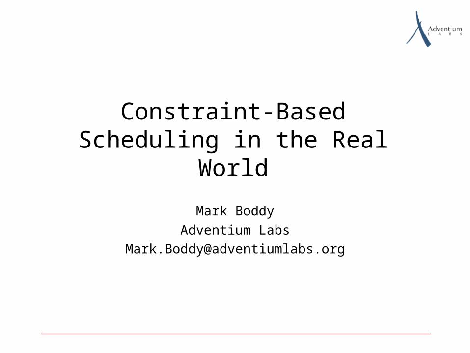
Finite-Capacity SchedulingSpecify activities linked to operations (transfers, tool changes, delivery dates, production runs, etc.).
This specification includes:
–Activity start and end times
–Resource usage, including raw materials, power, equipment needed, labor required
Finite capacity schedules can be used to determine predicted inventory levels, campaign completion/product delivery dates, economic performance, unit operating modes, and resource bottlenecks.
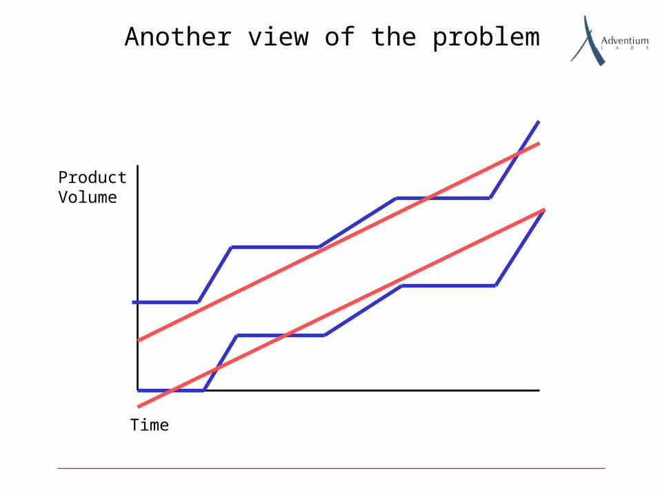
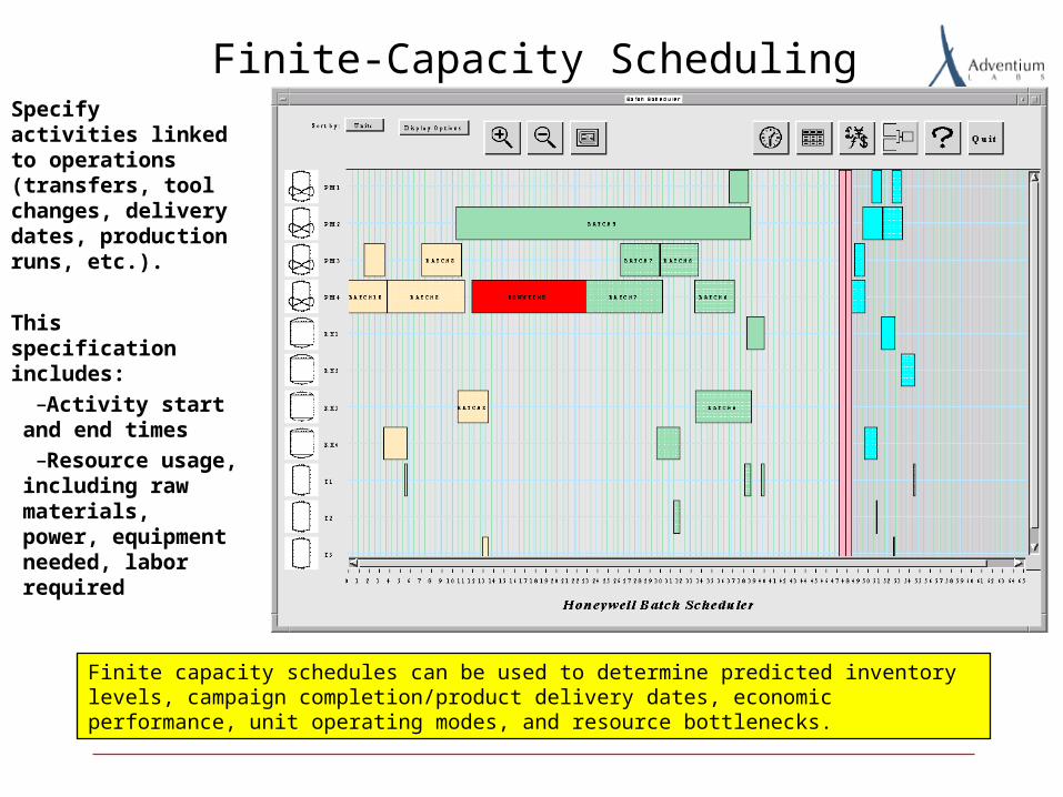
Another view of the problem
Time
ProductVolume
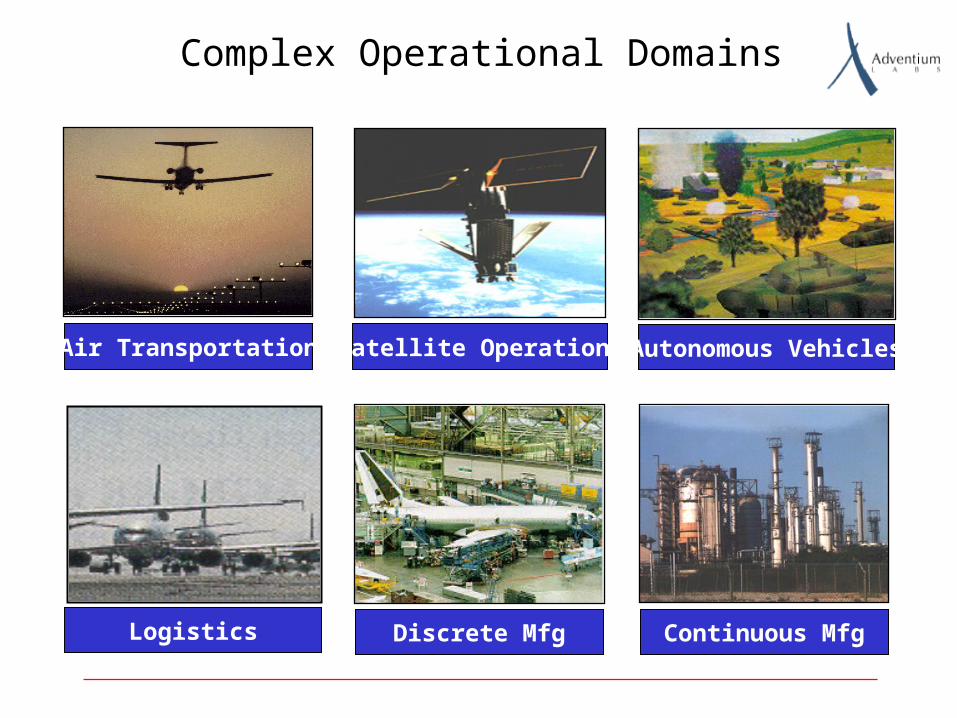
Complex Operational Domains
Air Transportation Satellite Operations Autonomous Vehicles
Continuous MfgDiscrete MfgLogistics
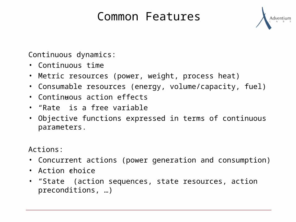
Common Features
Continuous dynamics:
• Continuous time
• Metric resources (power, weight, process heat)
• Consumable resources (energy, volume/capacity, fuel)
• Continuous action effects
• “Rate” is a free variable
• Objective functions expressed in terms of continuous parameters.
Actions:
• Concurrent actions (power generation and consumption)
• Action choice
• “State” (action sequences, state resources, action preconditions, …)
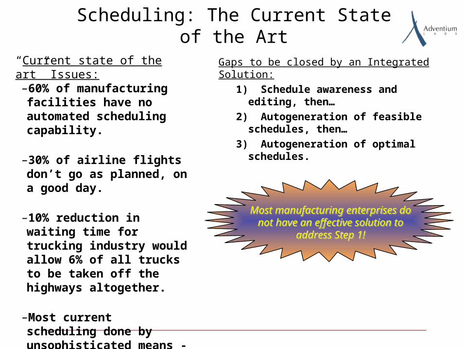
Scheduling: The Current State of the Art
“Current state of the art” Issues:–60% of manufacturing facilities have no automated scheduling capability.
–30% of airline flights don’t go as planned, on a good day.
–10% reduction in waiting time for trucking industry would allow 6% of all trucks to be taken off the highways altogether.
–Most current scheduling done by unsophisticated means - spreadsheets or manually.
Gaps to be closed by an Integrated Solution:
1) Schedule awareness and editing, then…
2) Autogeneration of feasible schedules, then…
3) Autogeneration of optimal schedules.
Most manufacturing enterprises do not have an effective solution to address Step
1!
Most manufacturing enterprises do not have an effective solution to address Step
1!
Value of Scheduling for Manufacturing• Reduce Costs
– Reduce disruption frequency and severity (what-if scenarios, detailed maintenance schedules)
– Improve parts/raw material ordering (better tracking of on-hand inventory)
– Reduce Work-In-Process inventory (reduced lot-rot, more timely vendor ordering, better synchronization of production to delivery dates)
– Reduce changeover costs (cleaning, new catalyst, temperature changes, …).
• Enhance Capital Investment Planning
– prioritize and quantify payoff for capital investment
• Increase Effective Capacity
– Identify and remove bottlenecks
– Increase agility (improve “Available to Promise”)
Determining when and how to accomplish some set of tasks.
The classic job shop:
• A set J of jobs to be run, each with
• a set of tasks to run in sequence, each on some unique element of
• a set M of machines
Common problem statements:
• Find a feasible schedule.
• Minimize makespan.
• Given a set of deadlines, minimize tardiness.
What is Scheduling?
Ti
Possible Complications (a brief sample)
• Choice of resource
• Other resource constraints
– (Global) capacity constraints
– Inter-activity constraints
– Consumable resources
• Complex temporal constraints (latency, preemption, hierarchical activity relationships).
• System dynamics (flow rates, chemical composition, …)
• Activity generation
• Reasoning about state
Effective Domain Modeling is Hard
Example: large transport pipelines
• Pipeline volume must be modelled explicitly (not like shipping and receiving).
• Currently model is to have slugs of material with associated volume, etc., plus a position in the pipeline.
• Material movement in the pipeline requires both input and output flows.
• Rate is independent of individual movements
How schedules are used is a factor as well
• Schedules are generated to satisfy existing plans.
• Schedules are generated in a historical context.
• Schedules are usually not constructed completely automatically.
• Schedules frequently require input from multiple parties.
• Schedules are used in operations.
– Updating, as events occur.
– Rescheduling, as conflicts are detected.
– Post mortem examinations.
• (Schedules are persistent artifacts.)
• Schedules are large.
• Optimization is important, but hard to formalize properly.
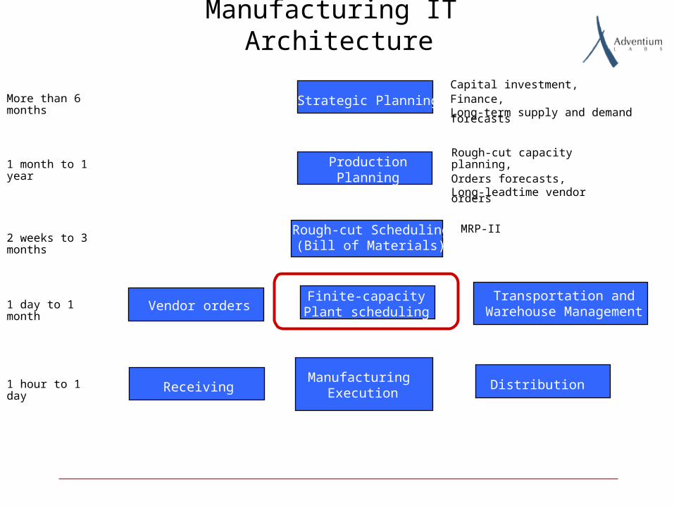
Manufacturing IT Architecture
Strategic Planning
ProductionPlanning
Finite-capacityPlant scheduling
Manufacturing Execution
Distribution
Capital investment, Finance, Long-term supply and demand forecasts
Rough-cut capacity planning, Orders forecasts,Long-leadtime vendor orders
Transportation andWarehouse ManagementVendor orders
Receiving
More than 6 months
1 month to 1 year
2 weeks to 3 months
1 day to 1 month
1 hour to 1 day
Rough-cut Scheduling(Bill of Materials)
MRP-II
Scheduling as a Constraint Satisfaction Problem
CSPs are specified as:
– A set V of variables
– A set C of constraints, each constraint a relation specifying tuples of permissible values for some subset of V.
The objective is to find a feasible (alt., optimal) complete assignment for V, consistent with C.
Advantages to a CSP approach
• Flexible, declarative representation.
• Lots of previous and current work on solution methods.
• General solution techniques:
– Static structural analysis
– Propagation
– Search
• Requirements and scheduling decisions can be represented as constraints.
Scheduling as Search Using a Dynamic CSP
CSP Variables:
– Activity start and end times
– Activity resource assignments
Constraints:
– Temporal constraints (duration, ordering, release times, deadlines, …)
– Resource constraints (permissible assignments, usage requirements, state information, ...)
– System dynamics (rate limitations, allowable state changes, …)
Search over:
– Activity generation
– Resource assignments
– Activity orderings, start and end times
Hybrid Systems
Hybrid systems have both continuous and discrete components, as opposed to:
– Combinatorial problems, such as knapsack, TSP, or jobshop
– Continuous problems, captured as sets of mathematical equations and inequalities.
Combinatorial, continuous, and hybrid constraint problems can all be framed in terms of either satisfiability (CSP) or optimality (COP).
Scheduling is a hybrid constraint problem.
Solving Hybrid Systems
MI(N)LP
– Discrete choices represented using integer variables.
– Continuous variables represented using equations and inequalities
– Typical solution methods involve iterating some form of relaxation to a purely continuous model, followed by forcing one or more integer variables to an integral value.
Hybrid CLP/MP approaches
– The problem is represented explicitly in two separate models, one a conventional mathematical program, the other a discrete CSP.
– Variants:
• Conditional math programming (Hooker, Grossman)
• Variable correspondence (Heipcke)
• Cooperating solvers (Ilog Solver)
Constraint Envelope Scheduling
A least commitment approach:
Accumulate additional constraints (e.g., activity orderings), so as to narrow the space of possible schedules, until all schedules in the remaining set are feasible.
Other people doing similar things:
– Nicola Muscettola et al.: HSTS/Europa
– Malik Ghallab: IxTeT
– Steve Smith: DITOPS
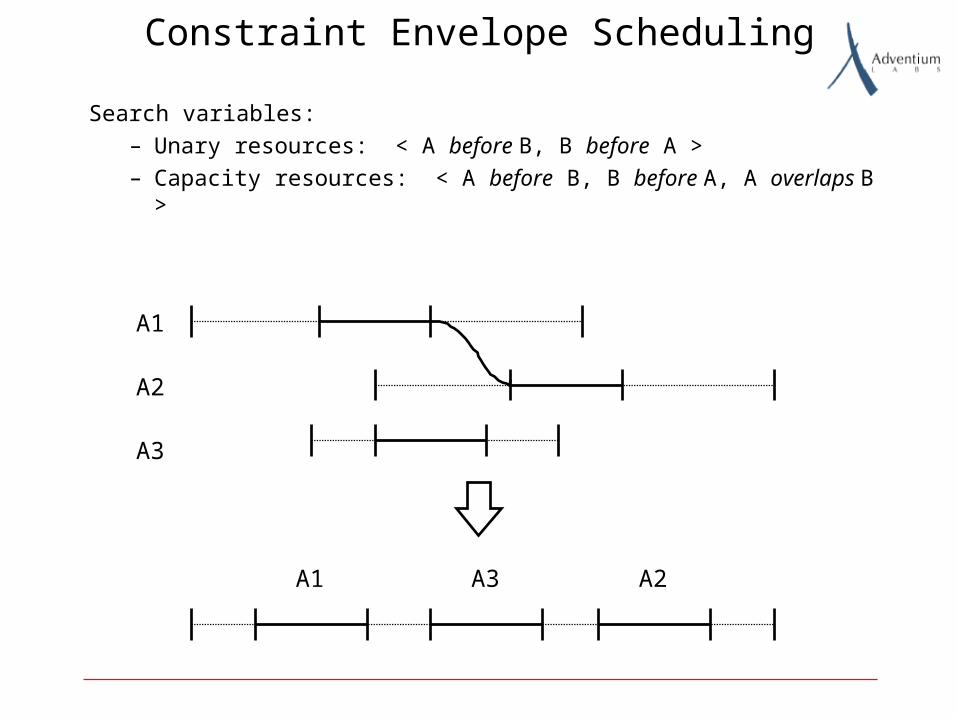
Constraint Envelope Scheduling
Search variables:
– Unary resources: < A before B, B before A >
– Capacity resources: < A before B, B before A, A overlaps B >
A1
A2
A3
A1 A2A3
Constraint Envelope Scheduling
Advantages:
– No premature commitment
– Flexible search strategies
– Natural representation for decisions (“do it before lunch”)
– Natural interleaving of search and propagation
Disadvantages:
– (Somewhat) cumbersome to implement.
– Intermediate results are less intuitive to users (more difficult to present, anyway).
– Efficiency concerns (a matter of degree…)
Constraint Envelope Scheduling Solver
A cooperating solver approach:
– Mathematical model is purely continuous, heavily optimized for speed and scaling.
– All interesting disjunction is captured in the discrete model.
– Standard architecture permits swapping of continuous solvers.
Requirements:
– Global consistency determination
– Incremental (or very fast) add and delete
– Culprit identification
Integrated continuous solvers:
– Simple Temporal Problem
– Linear solver
– Nonlinear solver

CES Solver Architecture
Discrete Constraint Engine
ContinuousConstraint Engine
1. Continuous constraints added as result of discrete decisions
2. Continuous constraint propagation and consistency check.
2.a. Propagation of additional constraints to discrete engine2.b. Propagation of additional constraints to continuous engine, repeat 2.a, 2.b as needed/desired
3. Discrete constraints added as result of continuous decisions
4. Discrete constraint propagation and consistency check.
4.a. Propagation of additional constraints to continuous engine4.b. Propagation of additional constraints to discrete engine,
repeat 4.a, 4.b as needed/desired
Three Different Continuous Solvers
The Simple Temporal Problem: constraints of the form P2 - P1 <= D.
– Inference supported: (dis)proving the consistency of a specified temporal relation between activity begin and end points.
– Implementation: shortest-path search in a graph.
• Up to 60,000 nodes (so far).
• Incremental consistency checking and propagation.
Linear solver: currently using Ilog CPLX
– Full, commercial linear solver.
– Solution times are a few milliseconds
– “Irreducible Infeasible Sets”
Nonlinear solver: locally developed “subdivision solver.”
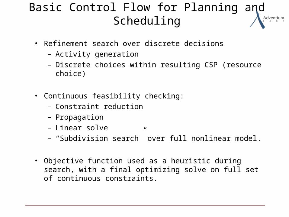
Basic Control Flow for Planning and Scheduling
• Refinement search over discrete decisions
– Activity generation
– Discrete choices within resulting CSP (resource choice)
• Continuous feasibility checking:
– Constraint reduction
– Propagation
– Linear solve
– “Subdivision search” over full nonlinear model.
• Objective function used as a heuristic during search, with a final optimizing solve on full set of continuous constraints.
Less and Less Commitment
For the past 13 years, our approach has been to shove as much into the continuous model as possible, without slowing it down.
– 50,000+ temporal constraints for SAFEbus avionics scheduling problem
– 18,000 continuous constraints (2700 quadratic) on 14,000 variables for scheduling an entire petroleum refinery
Why?
– Reduces backtracking due to premature commitment in discrete search
– Reduces size of discrete search, as well
– Resulting flexibility is useful for schedule updates and for optimization.
– Reduced need for explicit bookkeeping (we don’t keep resource timelines for consumable resources).
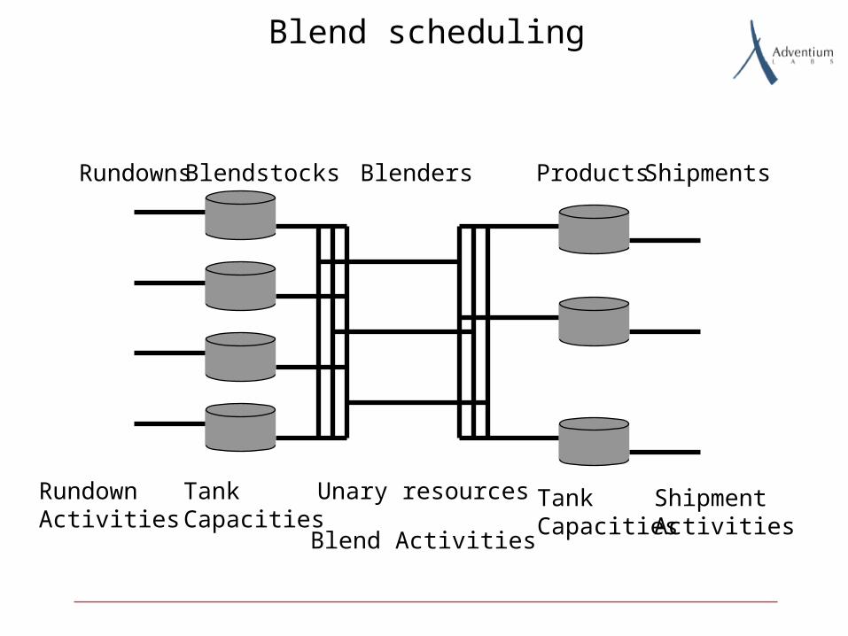
Blend scheduling
Rundowns Blendstocks Blenders Products Shipments
RundownActivities
TankCapacities
Unary resources
Blend Activities
TankCapacities
ShipmentActivities
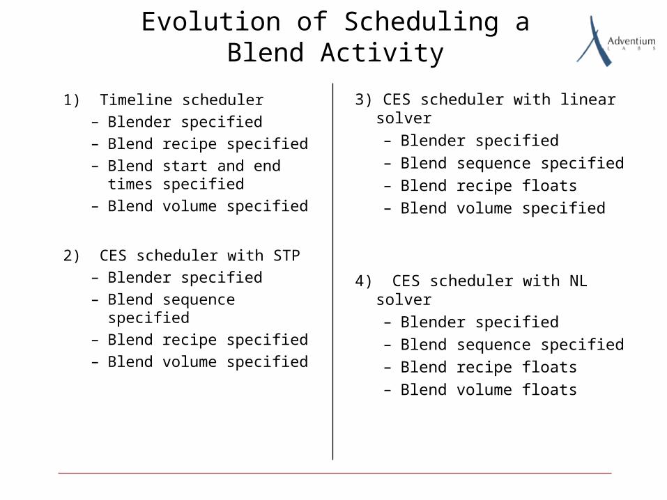
Evolution of Scheduling a Blend Activity
1) Timeline scheduler
– Blender specified
– Blend recipe specified
– Blend start and end times specified
– Blend volume specified
2) CES scheduler with STP
– Blender specified
– Blend sequence specified
– Blend recipe specified
– Blend volume specified
3) CES scheduler with linear solver
– Blender specified
– Blend sequence specified
– Blend recipe floats
– Blend volume specified
4) CES scheduler with NL solver
– Blender specified
– Blend sequence specified
– Blend recipe floats
– Blend volume floats
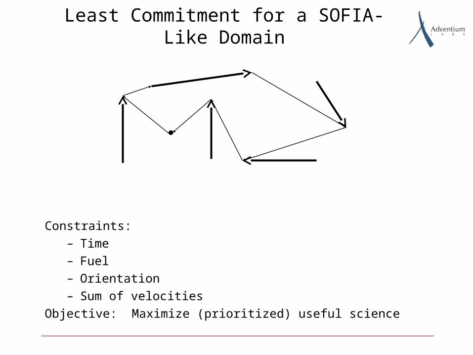
Least Commitment for a SOFIA-Like Domain
Constraints:
– Time
– Fuel
– Orientation
– Sum of velocities
Objective: Maximize (prioritized) useful science
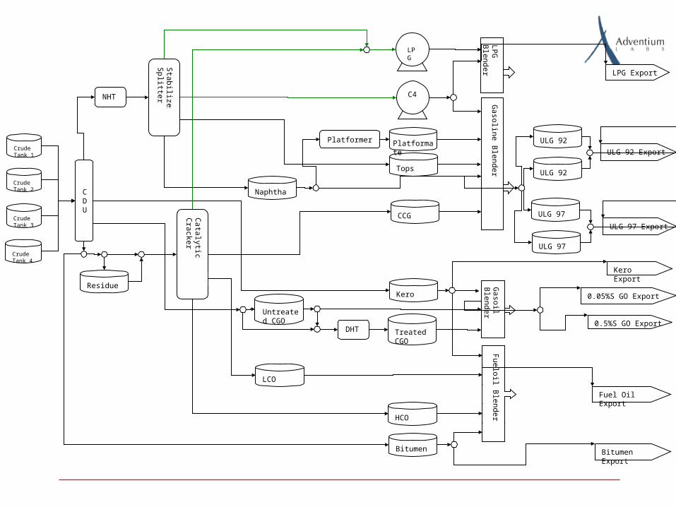
Crude Tank 1
Crude Tank 2
Crude Tank 3
Crude Tank 4
NHT
DHT
Naphtha
Tops
Platformer Platformate
LPG
C4
CCG
LCO
HCO
Untreated CGO
Treated CGO
KeroResidue
Bitumen
Gasoline B
lenderULG 92
ULG 97
ULG 97 Export
ULG 92 Export
Kero Export
LPG Export
LPG
B
lender
ULG 97
ULG 92
Gasoil
Blender
0.05%S GO Export
0.5%S GO Export
Fueloil B
lender Fuel Oil Export
Bitumen Export
CDU
Catalytic C
racker
Stabilizer/
Splitter
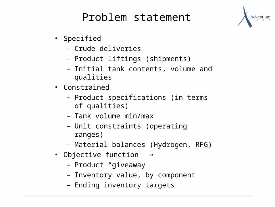
Problem statement
• Specified
– Crude deliveries
– Product liftings (shipments)
– Initial tank contents, volume and qualities
• Constrained
– Product specifications (in terms of qualities)
– Tank volume min/max
– Unit constraints (operating ranges)
– Material balances (Hydrogen, RFG)
• Objective function
– Product “giveaway”
– Inventory value, by component
– Ending inventory targets
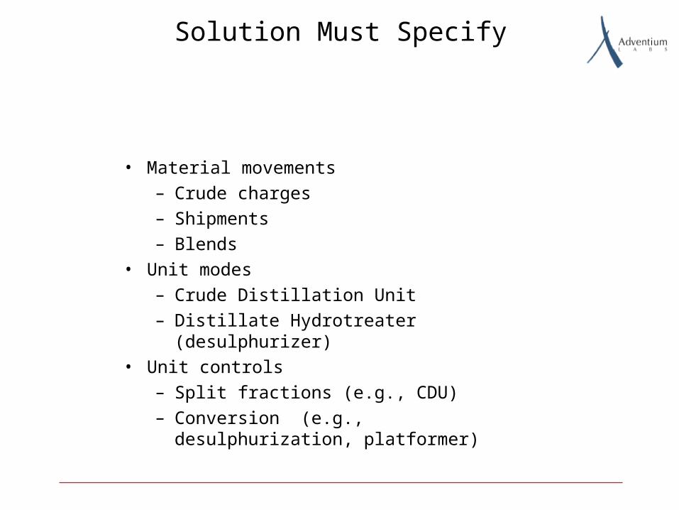
Solution Must Specify
• Material movements
– Crude charges
– Shipments
– Blends
• Unit modes
– Crude Distillation Unit
– Distillate Hydrotreater (desulphurizer)
• Unit controls
– Split fractions (e.g., CDU)
– Conversion (e.g., desulphurization, platformer)

Mathematical Nature of the Problem
• Any model with variable properties and flow or tank mixing requires bilinear equations, which are therefore quadratic.
• Systems of quadratic equations can represent any polynomial or rational function, and can approximate any nonlinear function to arbitrary accuracy.
• Systems of quadratic equations are not equivalent to quadratic programs, which have linear equations, only the objective is quadratic.
• Quadratic and bilinear systems typically show multiple local minima in optimization problems.
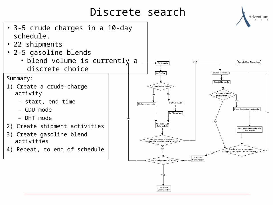
Discrete search
Summary:
1) Create a crude-charge activity
– start, end time
– CDU mode
– DHT mode
2) Create shipment activities
3) Create gasoline blend activities
4) Repeat, to end of schedule
• 3-5 crude charges in a 10-day schedule.• 22 shipments• 2-5 gasoline blends
• blend volume is currently a discrete choice
Continuous model
• Activity start and end times (interval model)
• Process unit control settings
• Flow volumes and rates
• Flow qualities
• Tank volumes and qualities as a function of time (at activity endpoints)
• Both mass and volume are tracked
– Some unit controls affect Specific Gravity
– Products may be sold by weight, by volume, or both.
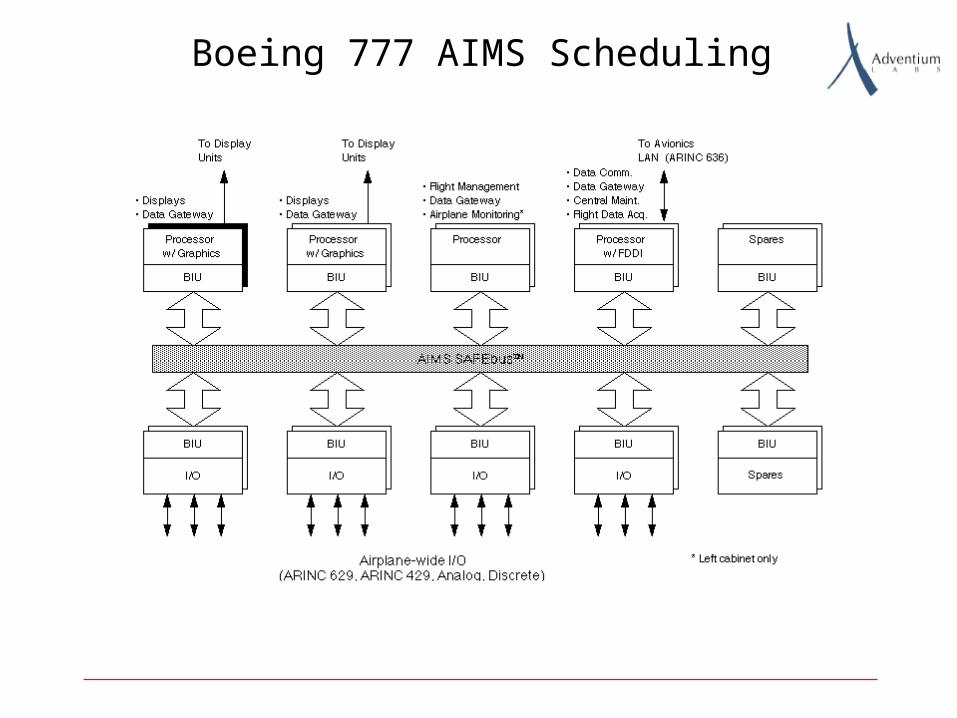
Boeing 777 AIMS Scheduling
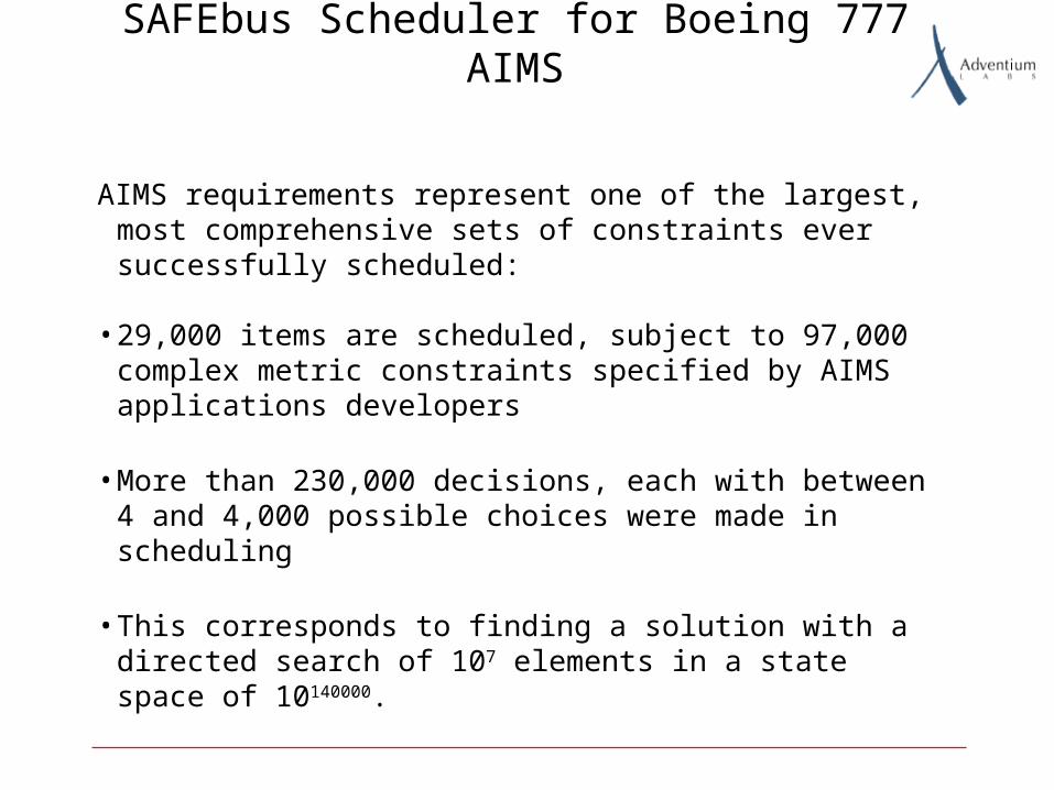
SAFEbus Scheduler for Boeing 777 AIMS
AIMS requirements represent one of the largest, most comprehensive sets of constraints ever successfully scheduled:
• 29,000 items are scheduled, subject to 97,000 complex metric constraints specified by AIMS applications developers
• More than 230,000 decisions, each with between 4 and 4,000 possible choices were made in scheduling
• This corresponds to finding a solution with a directed search of 107 elements in a state space of 10140000.
How We Solved It
Ginsberg’s “Dynamic Backtracking” algorithm
• Published in 1994
• We fixed a bug
• We extended it
Moral: sometimes the path from research to product takes months, not years.
Concluding Remarks
• Theoretical results and algorithms from CSP/COP are frequently of great practical use.
• But, they are almost never of use unaltered.
• And they are almost never of use in isolation.
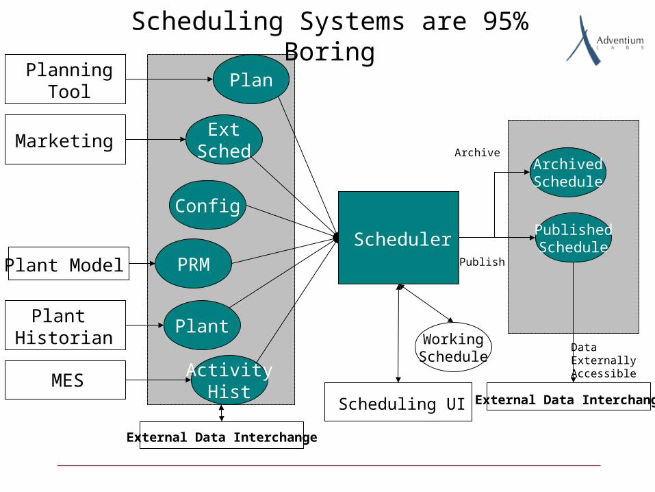
Scheduling Systems are 95% Boring
PRM
Config
Plan
ExtSched
Plant
ActivityHist
WorkingSchedule
Scheduler
PlanningTool
Marketing
Plant Model
Plant Historian
MES
External Data Interchange
PublishedSchedule
ArchivedSchedule
Scheduling UI
Publish
Archive
DataExternallyAccessible
External Data Interchange
Areas for Further (Interesting!) Work
• Optimal Scheduling (for the right definition of “optimal”)
• Incorporating probabilities
• Robust schedules vs. responsive schedulers
• Moving up into production planning
• Better integration with action selection and states (but see workshops at ICAPS-04, ICAPS-05)