Consolidations Fiscal Multipliers and Fiscal Fiscal ......ECO/WKP(2012)10 2 ABSTRACT/RESUMÉ Fiscal consolidation Part 2. Fiscal multipliers and fiscal consolidations This paper looks

Please cite this paper as:

Barrell, R., D. Holland and I. Hurst (2012), “FiscalConsolidation: Part 2. Fiscal Multipliers and FiscalConsolidations”, OECD Economics Department WorkingPapers, No. 933, OECD Publishing.http://dx.doi.org/10.1787/5k9fdf6bs78r-en

OECD Economics DepartmentWorking Papers No. 933

Fiscal Consolidation: Part 2.Fiscal Multipliers and FiscalConsolidations

Ray Barrell, Dawn Holland, Ian Hurst

JEL Classification: E17, E37, E62

http://dx.doi.org/10.1787/5k9fdf6bs78r-en

Unclassified ECO/WKP(2012)10 Organisation de Coopération et de Développement Économiques Organisation for Economic Co-operation and Development 22-Feb-2012 ___________________________________________________________________________________________

English - Or. English ECONOMICS DEPARTMENT

FISCAL CONSOLIDATION PART 2. FISCAL MULTIPLIERS AND FISCAL CONSOLIDATIONS ECONOMICS DEPARTMENT WORKING PAPER No. 933

by Ray Barrell, Dawn Holland and Ian Hurst

All Economics Department Working Papers are available through OECD's internet website at www.oecd.org/eco/workingpapers JT03316447

Complete document available on OLIS in its original format This document and any map included herein are without prejudice to the status of or sovereignty over any territory, to the delimitation of international frontiers and boundaries and to the name of any territory, city or area.

ECO

/WK

P(2012)10 U

nclassified

English - O

r. English

ECO/WKP(2012)10

2

ABSTRACT/RESUMÉ

Fiscal consolidation Part 2. Fiscal multipliers and fiscal consolidations

This paper looks at various aspects of fiscal consolidation in 18 OECD economies. The prospects for fiscal consolidation depend upon the problems the country may face with its debt stock, the political will to deal with these problems and on the costs of consolidation. The analysis is based on a series of simulations using the National Institute Global Econometric Model, NiGEM. The properties of the NiGEM model are discussed first. Although the model is estimated it has a strong role for expectations and can be run under different modes of expectations formation. This allows a decomposition of the factors that might affect the results. Temporary and permanent shifts in fiscal policy are assessed as well as the potential impact of fiscal consolidation plans under different monetary and fiscal feedback rules and different modes of expectations formation. If fiscal policy is expected to be tightened in the future, then long rates will fall now, and perhaps even induce a short-term expansion of output. Expansionary fiscal contractions of this sort are rare, however, and none are anticipated with the programmes that are investigated.

JEL classification codes: E17; E37; E62

Key words: Large scale structural macro models; fiscal multipliers; rational expectations; budget consolidation in the OECD

++++++++++++++++++++

Consolidation budgétaire Partie 2. Multiplicateurs budgétaires et assainissement des finances publiques

Ce document examine divers aspects de l’assainissement des finances publiques dans 18 pays de l’OCDE. Le potentiel de consolidation budgétaire dépend du montant de la dette d’un pays et des problèmes qui peuvent en résulter, de la volonté politique de traiter ces problèmes et des coûts du redressement. L’analyse s’appuie sur un ensemble de simulations fondées sur le modèle économétrique mondial de l'Institut de recherche économique et sociale du Royaume-Uni (NiGEM). Les auteurs examinent en premier lieu les caractéristiques du modèle NiGEM. Même si ce modèle procède par estimation, il conditionne fortement les anticipations et peut être appliqué à différents modes de formation des anticipations. Cela permet de décomposer les facteurs susceptibles d’influer sur les résultats. Les auteurs évaluent ensuite les modifications temporaires et permanentes de la politique budgétaire, ainsi que l’impact potentiel des plans de redressement budgétaire selon différentes règles de rétroaction budgétaire et monétaire et différents modes de formation des anticipations. Si l’on s’attend à un durcissement de la politique budgétaire à l’avenir, les taux longs baisseront immédiatement, ce qui pourrait même induire une expansion à court terme de la production. Néanmoins, les contractions budgétaires expansionnistes de ce type sont exceptionnellement rares, et les programmes étudiés n’en prévoient aucune. Classification JEL : E17 ; E37 ; E62

Mots-clés : Modèles macroéconomiques structurels à grande échelle ; multiplicateurs budgétaires ; anticipations rationnelles ; redressement budgétaire dans l’OCDE

© OECD (2012) You can copy, download or print OECD content for your own use, and you can include excerpts from OECD publications, databases and multimedia products in your own documents, presentations, blogs, websites and teaching materials, provided that suitable acknowledgment of OECD as source and copyright owner is given. All requests for commercial use and translation rights should be submitted to [email protected].

mailto:[email protected]�

ECO/WKP(2012)10

3

TABLE OF CONTENTS

FISCAL CONSOLIDATION PART 2. FISCAL MULTIPLIERS AND FISCAL CONSOLIDATIONS ..................................................... 5

Introduction .................................................................................................................................................. 5 The NiGEM model ...................................................................................................................................... 6

Consumer behaviour ................................................................................................................................ 7 Prices ........................................................................................................................................................ 7 Government sector ................................................................................................................................... 8 Monetary policy ....................................................................................................................................... 9 Forward looking financial markets ........................................................................................................... 9

Fiscal multipliers ........................................................................................................................................ 10 Multiplier profiles for different fiscal instruments .................................................................................... 15 US fiscal multipliers under different monetary policy rules ...................................................................... 19 Fiscal multipliers and expectations ............................................................................................................ 21 Government debt and consolidation programmes ..................................................................................... 22 Assessing fiscal consolidation programmes until 2012 ............................................................................. 32 Further consolidation needs beyond 2012 ................................................................................................. 36 Conclusion ................................................................................................................................................. 40

Bibliography .................................................................................................................................................. 40

Tables

1. First-year multipliers from 1% of GDP temporary innovations .......................................................... 12 2. Key factors determining cross-country differences in multipliers ...................................................... 13 3. First-year multipliers from 1% of GDP permanent consolidation ...................................................... 14 4. Projections for government deficits underlying the stochastic simulations ........................................ 23 5. Stochastic bounds around debt stock projections in 2016 ................................................................... 23 6. Impacts of rules on distance of 95% bound from baseline .................................................................. 32 7. Fiscal impulses 2010-12 ...................................................................................................................... 33 8. Expected deficit and debt stock in 2012 .............................................................................................. 37

Figures

1. Temporary spending multiplier and import penetration ...................................................................... 14 2. Permanent and temporary spending multipliers against economy size ............................................... 15 3. Permanent multipliers in the US ......................................................................................................... 16 4. Permanent multipliers for the UK ....................................................................................................... 17 5. Permanent multipliers for Germany .................................................................................................... 17 6. Permanent multipliers for France ........................................................................................................ 18 7. Permanent multipliers for the Netherlands .......................................................................................... 18 8. US fiscal consolidation multipliers – different initial reactions .......................................................... 19 9. US fiscal consolidation multipliers – impacts using different monetary policy feedback rules ......... 20 10. Impact of the zero lower bound on interest rates on the US consolidation multiplier ........................ 21 11. The impact of expectations on the US multiplier ................................................................................ 22

ECO/WKP(2012)10

4

12. Bounds around debt stock projections ................................................................................................ 24 13. Stochastic bounds around the euro area budget deficit ....................................................................... 28 14. Stochastic bounds around debts and deficits for Germany, Italy and France for a 1% of GDP spending based consolidation scenario .............................................................................................. 29 15. The effect of unilateral scenarios ........................................................................................................ 35 16. Impact of joint policy action relative to unilateral action ................................................................... 36 17. Short and long-run impact of fiscal consolidation on the long-term real rate from 2013 ................... 37 18. The impact of implementing necessary fiscal consolidation from 2013 on GDP ............................... 38 19. Global consolidation ........................................................................................................................... 39 20. Euro Area consolidation ...................................................................................................................... 39

ECO/WKP(2012)10

5

F I SC AL C ONSOL I DAT I ON

PAR T 2. F I SC AL M UL T I PL I E R S A ND F I SC AL C ONSOL I DAT I ONS

By Ray Barrell, Dawn Holland and Ian Hurst1

Introduction

This paper assesses various fiscal consolidation aspects for 18 OECD economies. The prospects for fiscal consolidation depend upon the problems a country may face with its debt stock, the political will to deal with these problems and on the costs of consolidation. These costs are a function of the impacts of fiscal policy on the economy. The analysis is based on a series of simulations using the National Institute Global Econometric Model, NiGEM. The NiGEM model will be discussed first, as the results depend upon the model properties. The key features of the model are that it is estimated and has a common structure across the 18 countries. If the results differ across countries it will be because they are different. Some of these differences, such as the openness of the economy, are important. They change over time and they are not related to estimation. Others, such as the speed of response to changes in income, do depend upon how the model was estimated. Although the model is estimated it has a strong role for expectations, and it is also flexible, as it can be run under different models of expectations formation, depending upon the thought experiment being undertaken.

Then the factors that might affect the results will be decomposed, for instance, by looking at temporary and permanent shifts in fiscal policy. In each case the first year multipliers will be presented. In the first year taxes will be raised or spending cut so that ex ante the deficit would improve by 1% of GDP. Government consumption on goods and services and government transfers to individuals (mainly benefits and state pensions) will be changed, as well as income tax and indirect taxes. In the latter two the tax rate will be changed, and this has implications elsewhere in the economy. Each experiment is undertaken with the same set of assumptions, which will be discussed. The effects of government investment or corporate taxes will not be investigated. Government investment and corporate tax receipts are generally a small proportion of the economy, and a 1% of GDP change to either would be a large proportionate change. In a temporary shock, the impact of a shift in government investment would be the same as a government consumption shock of the same magnitude. A long run shock to either government investment or the corporate tax rate would change the real equilibrium of the economy.

When undertaking experiments it is important to be able to dissect the contributing factors. These will be decomposed by removing them or changing them one at a time. Models such as NiGEM have to run with a monetary and a fiscal feedback rule and they use rational expectations. The rules and the assumptions about expectations affect outturns. The effects of different rules and the impacts of the 1. The authors are outside consultants to the OECD Economics Department. Ray Barrell is Professor at

Brunel University; Dawn Holland and Ian Hurst are Senior Research Fellows at the National Institute of Economic and Social Research. This is one of the background papers for the OECD’s project on Fiscal Consolidation. The authors wish to thank Jean-Luc Schneider, Peter Hoeller and Douglas Sutherland for helpful comments on earlier drafts. They also wish to thank Susan Gascard for administrative and editorial support.

ECO/WKP(2012)10

6

assumptions will be investigated, looking at the role of forward looking bond and exchange rate markets, forward looking equities, forward looking wage bargainers and forward looking consumers. It is possible to run NiGEM with some or all of these, the effects on the multipliers will be investigated. Multipliers are time and state dependent. As we showed in Barrell, Fic and Liadze (2009), they are smaller the more open the economy and they appear to have been falling over time. They depend on the offsetting feedbacks in the economy, and in particular on the offsetting reactions of interest rates. A tighter fiscal policy will allow short-term interest rates to be lower now and in the future if there is no change to the monetary policy target, and hence long-term interest rates will be lower now. And the exchange rate will fall. Equity prices will rise and forward looking wage bargainers will change their behaviour. Each of these helps offset the contractionary effects of fiscal consolidation. It is also possible that the timing of fiscal consolidation and type of rule applied may affect outcomes. If fiscal policy is expected to be tightened in the future then long rates will fall now, increasing the offset, and perhaps even inducing a short-term expansion of output. Expansionary fiscal contractions are exceptionally rare, however.

Then the evolution of debt stocks in the NiGEM baseline is assessed, the fiscal packages announced up until December 2010 are implemented and deficit targets after 2012 are added that have to be met by changing direct tax rates.2

The NiGEM model

Probability bounds are put around these estimates and the impact of any further measures that may have to be enacted to achieve the targets set for deficits is assessed. The effects of these consolidation programmes are simulated, removing them and seeing what the outturn might be. Then imposing an additional target for the deficit of 1.5% of GDP is discussed. This is done globally and in each major area. This would require a significant fiscal tightening in the United States and Japan.

The National Institute’s global econometric model (NiGEM) can be used in a number of ways, from a backward looking structural model to a version that has similar long-run properties as the dynamic stochastic general equilibrium models used by institutions such as the Bank of England.3

GDP (Y) is determined in the long run by supply factors, and the economy is open and has perfect capital mobility. The production function has a constant elasticity of substitution between factor inputs, where output depends on capital (K) and on labour services (L), which is a combination of the number of persons in work and the average hours of those persons. Technical progress (tech) is assumed to be labour augmenting and independent of the policy innovations considered here.

ρρλρ δδγ /1)))(1()(( −−− −+= techLLeKY (1)

In general, forward looking behaviour in production is assumed and because of ‘time to build’ issues investment depends on expected trend output four years ahead and the forward looking user cost of capital. However, the capital stock does not adjust instantly, as there are costs involved in doing so that are represented by estimated speeds of adjustment. The equilibrium level of unemployment is the outcome of the bargaining process in the labour market, as discussed in Barrell and Dury (2003), and the speed of adjustment depends on (rational) expectations of future inflation unless backward oriented learning is used. Financial markets normally follow arbitrage conditions and they are forward looking. The exchange rate, the long-term interest rate and the equity price will all ‘jump’ in response to news about future events. Fiscal policy making involves gradually adjusting direct taxes to maintain the deficit on target, but it is

2. The data used in the simulations are those available in the first half of 2011.

3. The Bank of England Quarterly model is discussed in Harrison et al. (2005). NiGEM is discussed in Barrell, Holland and Hurst (2007), Barrell, Hurst and Mitchell (2007) and in other papers at www.niesr.ac.uk. NiGEM does not impose maximising equilibrium conditions in the same way as Dynamic Stochastic General Equilibrium models, but has the same steady-state equilibrium properties.

ECO/WKP(2012)10

7

assumed that taxes have no direct effect on labour supply decisions. Monetary policy making involves targeting inflation with an integral control from the price level, as discussed in Barrell, Hall and Hurst (2006) and inflation settles at its target in all simulations. Some of the key features of the model that determine the outturns of the simulation studies are detailed further below.

Consumer behaviour

As Barrell and Davis (2007) show, both the level of total asset based wealth (ln(TAW) or ln(NW+HW)) and changes in financial (dln(NW)) and especially housing wealth (dln(HW)) will affect consumption (C).4

Their estimates suggest that the impact of changes in housing wealth have five times the impact of changes in financial wealth in the short run, although long-run effects are the same. Barrell and Davis (2007) also show that adjustment to the long-run equilibrium shows some inertia as well. Al Eyd and Barrell (2005) discuss borrowing constraints, and investigate the role of changes in the number of borrowing constrained households. It is common to associate the severity of borrowing constraints with the coefficient on changes in current real incomes (dln(RPDI)) in the equilibrium correction equation for consumption. These coefficients are important in evaluating impact multipliers. One can write the equation for dln(C) as

( ) ( ) ( ) ( ) ( )[ ]{ }( ) ( ) ( )ttt

tttt

HWdbNWdbRPDIdbRPDIbTAWbaCCd

lnlnlnln1lnlnln

321

10101

+++−++−= −−−λ

(2)

where the long-run relationship between ln(C) and ln(RPDI) and ln(TAW) determine the equilibrium savings rate, and this relationship forms the long-run attractor in an equilibrium correction relationship. The logarithmic approximation is explained in Barrell and Davis (2007).

Operating in forward-looking consumption mode, consumers react to the present discounted value of their future income streams, which is approximated by total human wealth (TW), although borrowing constraints may limit their consumption to their personal disposable income in the short run. Total human wealth is defined as

))1)(1/((1 tttttt myrrTWTYTW +++−= + (3)

Y is real income, T are real taxes, and the subscript t+1 indicates an expected variable which is discounted by the real interest rate rrt and by the myopia premium of consumers, myt. The equation represents an infinite forward recursion, and permanent income is the sustainable flow from this stock.

Prices

Consumer prices (CED) are modelled as a dynamic weighted average of unit costs of production and import prices, adjusted by the indirect tax rate. A policy shift that changes the indirect tax rate, therefore, has a direct impact on the price level. Unit costs of production (UTC) are derived from the cost minimization problem around the underlying production function, given by:

Minimize rKWLC += (4)

s.t. ρρλρ δδγ /1)))(1()(( −−− −+= techLLeKY (5)

4. Throughout d is the change operator and ln is the natural logarithm.

ECO/WKP(2012)10

8

where the factors of production L and K are associated with factor prices W (wages) and r (user cost of capital).

The first order conditions of the cost minimisation problem give the optimal input ratio, which can be substituted into the production function to derive the cost minimising levels of factor inputs to produce a given level of output. It is assumed that firms operate on their factor demand curves, at least in the long run, which leads to the following expression for marginal costs:

( ) ( ) ( ) techLYWMC Lρλρθ +

+−+= ln1lnln 1 (6)

where ( ) ( )δγρθ −−= 1lnln1 (7)

Marginal costs are treated as a shadow price, whereas observed basic prices (P) incorporate an endogenous mark-up, which is modelled as a function of the output gap.

Government sector

In order to evaluate multipliers a reasonably disaggregated description of both spending and tax receipts is needed. Corporate (CTAX) and personal (TAX) direct taxes and indirect taxes (MTAX) on spending are modelled, along with government spending on investment (GI) and on current consumption (GC), and transfers (TRAN) and government interest payments (GIP) are separately identified. Each source of taxes has an equation applying a tax rate to a tax base (profits, personal incomes or consumption). As a default, government spending on investment and consumption are rising in line with trend output in the long run, with delayed adjustment to changes in the trend. They are re-valued in line with the consumers’ expenditure deflator (CED). Government interest payments are driven by a perpetual inventory of accumulated debts. Transfers to individuals are composed of three elements, with those for the inactive of working age and the retired depending upon observed replacement rates. Spending less receipts gives the budget deficit (BUD), which adds to the debt stock.

BUD =CED*(GC+GI)+TRAN+GIP-TAX-CTAX-MTAX (8)

It has to be considered how the government deficit (BUD) is financed. Either money (M) or bond financing (DEBT) are allowed:

BUD = d(M) + d(DEBT) (9)

and rearranging gives:

DEBT= DEBTt-1 + BUD - d(M) (10)

In all policy analyses a tax rule is used to ensure that governments remain solvent in the long run. The default rule is applied to the personal direct tax rate, which is adjusted endogenously to bring the government deficit into line with a specified target. This ensures that the deficit and debt stock return to sustainable levels after a shock. A debt stock target can also be implemented and this is discussed below. The income tax rate (TAXR) equation is of the form:

TAXR = f(target debt or deficit ratio - actual debt or deficit ratio) (11)

If the government budget deficit is above the target, (e.g. 3% of GDP and the target is 1%) then the income tax rate is increased.

ECO/WKP(2012)10

9

Monetary policy

Interest rates are set by the monetary authority in relation to a targeting regime, where policy interest rates are set in relation to a rule that is normally forward looking. We distinguish two types of rules, those that target only inflation and those that target the price level or a nominal variable such as GDP or the money stock. During the “great moderation” era central bankers and many economists became convinced that they had changed the world they lived in by adopting simple feedback rules for monetary policy in combination with rules for fiscal policy that kept debt in bounds. The simple feedback rule was based on the Taylor Rule (TR) that suggests that when inflation increases the central bank should increase the interest rate more than in proportion to the rise in inflation, and hence the real interest rate would rise and help choke off demand. In a forward looking world it is possible to improve on this principal. If agents see the central bank as fully credible, then the announcement of a price level target (PLT), rather than just an inflation target, will stabilise fluctuations in output and in inflation. A price level targeting central bank will loosen policy more rapidly as it has to get the price level back to target. The converse will be true in a boom. These two feedback rules are shown in equation (12) below, with int being the intervention rate, ssr being the steady state (endogenous) real interest rate, og being the output gap, inf and inft being the inflation rate and the target, and P and PT being the price level and the price level target.

( ) ( )tttttt PTPainftinfaogassraaint −+−+++= + 413210 (12)

In a Taylor Rule a0 is zero, a1 is 1.0, a2 is 0.5, a3 is 1.5 and a4 is zero, whilst in a PLT regime a(1) is zero, a(2) is also zero, and a(3) is set to 0.7 and a(4) to 0.4. The PLT rule has the advantage of working only on observables. The same is true of a two pillar strategy as embraced by the ECB. The bank responds to deviations of inflation from target and also deviations of a nominal aggregate (NOM) – the money stock for instance – as described in equation:

( ) ( )tttt NOMTNOMbinftinfbbint −+−+= + 2110 (13)

Forward looking financial markets

A deflationary shock such as a fiscal tightening will have a weaker interest rate response under a Taylor Rule than under price level targeting, and both may be weaker than a two pillar rule. If actors know the rule is in place then they will form expectations of the future path of short rates, and this will cause the current long rate to change, along with the exchange rate and the equity price. Forward looking long rates (LR) should be related to expected future short-term rates:

( ) ( )∏ = ++=+T

jT

jtt intLR1

/111 (14)

Forward looking equity prices (EQP) are related to future profits (PR) in a forward recursion where eprem is the equity premium

( )( )tt

ttt epremint

EQPPREQP

+++= +

111 (15)

The exchange rate depends on the expected future path of interest rates and the exchange rate risk premia, solving an uncovered interest parity condition, so that the expected change in the exchange rate is given by the difference in the interest earned on assets held in local and foreign currencies:

ECO/WKP(2012)10

10

( )tt

ttt rpee +

++

= + 1int1int1 *

1 (16)

where et is the bilateral exchange rate at time t (defined as domestic currency per unit of foreign currency), intt is the short-term nominal interest rate at home set in line with a policy rule, intt* is the interest rate abroad and rpt is the exchange rate risk premium.

Fiscal multipliers

NiGEM is an estimated and calibrated model with a supply side and rational expectations, but is does not go as far in this direction as modern DSGE models which are theory based, but fail in their description of the world. In a model such as ours multipliers are small. They average around 0.3 or less, as can be seen from Tables 1 and 3 below. Even then these estimates probably exceed the multipliers that one would see with any actual consolidation programme, because for some actions implementation speed is faster in the model than in the world. If one allows for more gradual implementation, this would reduce average multipliers to below 0.2. This matters in particular when comparing multipliers for taxes and benefits to those for spending. Taxes or benefits can be cut by 1% of GDP relatively easily both in the model and in the world. Multipliers in response to income tax and benefit adjustments are small, as a part of the decline in personal sector income is offset by a temporary adjustment in the savings rate. As one can see from the tables, multipliers appear larger for cuts in real government spending. This is in part because of the assumption that such cuts can be implemented immediately, and this is certainly not the case. It is also in part because government consumption is part of the income identity and hence when they are cut (and reduce the number of people employed or goods and services bought) measured real output falls. If one were to reduce government spending by as much, but do it through wage reductions, then the impact on real GDP would be much less, and the second round effects of the shock would effectively be the same as an increases in taxes.

In order to determine the effects of an ex ante change in fiscal policy one has to avoid offsetting or reinforcing policy effects, but the model must otherwise be allowed to run. In each of our simulations in this section we make the following assumptions:

• Policy reactions are turned off for the first year:

− The central bank does not change the short-term interest rate for a year, whatever the shock. It then follows a targeting regime that stabilises either the inflation rate or the price level.

− The government does not target the deficit for the first year. The model has a feedback rule which adjusts the direct tax rate in relation to the gap between actual and target deficits. This is switched off for a year.

− Government investment is fixed at the baseline for a year and does not respond to long-term factors in the first year. The same, where this is appropriate, is true for government consumption.

− Other tax rates and all benefit replacement rates are held constant throughout the simulation period.

• Markets work and all quantities and prices can react and there are no exogenous variables in the model, with the exceptions of policy targets, labour supply and risk premia:

ECO/WKP(2012)10

11

− Financial markets look forward and are assumed to follow arbitrage paths, and expectations for those paths are outturn consistent.

Long-term government bond rates are the forward convolution of future short- term policy rates plus an exogenous premium.

Long-term real interest rates are the forward convolution of future short-term real policy rates plus an exogenous risk premium made up of the bond premium plus private sector risks.

Equity prices are the discounted value of future profits, where the discount factor is the market interest rate plus the exogenous equity premium.

Exchange rates “jump” when future interest rates change and they follow the arbitrage path given by nominal interest rates.

− Labour markets are described by an exogenous labour supply, a labour demand equation and by a wage equation based on search theory, where the bargain depends on backward and forward looking inflation expectations.

− Capital stocks adjust slowly towards that associated with expected capacity output four years ahead, which in turn depends upon a forward looking user cost of capital. Expectations are rational and factor demands and capacity output are based on a CES production function.

− Consumers respond to their forward looking financial wealth, but are not fully forward looking.

In the next sections the implications of several of these default assumptions will be tested.

Table 1 reports the estimates of the first year multipliers for 18 OECD countries, under the default assumptions described above, for a 1% (ex ante) GDP rise in taxes or cut in spending that is reversed after one year. The multipliers for cuts in government consumption spending and spending on benefits are reported, as well as for rises in indirect taxes and direct (personal) taxes. Simulations are run one country at a time, so there are no spillovers across countries in the reported multipliers. Generally multipliers peak in the first year and then decline, and the ex post improvement in government revenues will normally be less than 1% of GDP as tax bases change. Some of the effects of the impulse will be offset by declines in interest rates. Both short and long rates should fall, but the former may be trapped at the lower bound at present. This will have a limited impact on our results as long rates are forward looking and can move even when current short rates are restrained by the zero bound. In NiGEM, investment behaviour is mainly influenced by long real rates through the user cost of capital, and these are free to fall in response to the temporary fiscal tightening.

ECO/WKP(2012)10

12

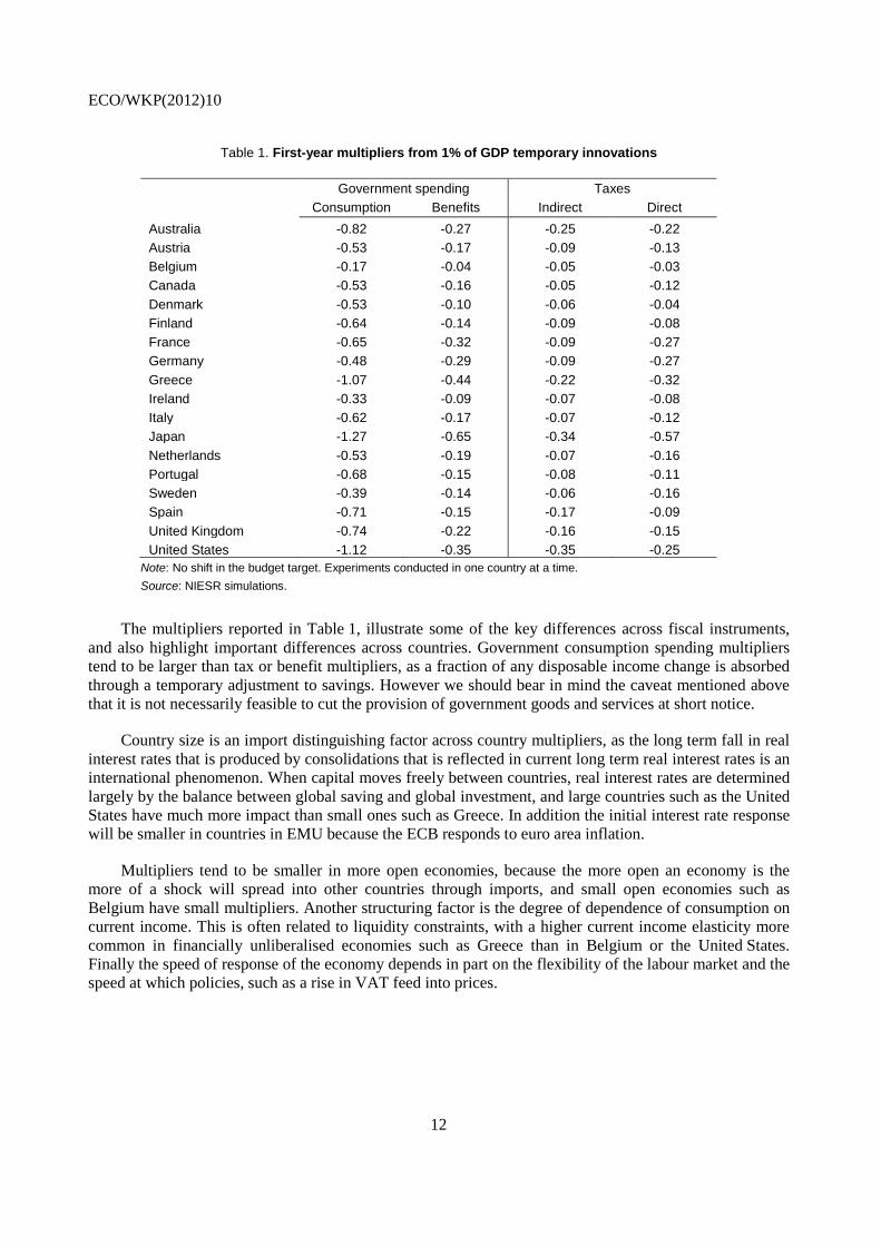
Table 1. First-year multipliers from 1% of GDP temporary innovations

Government spending Taxes Consumption Benefits Indirect Direct

Australia -0.82 -0.27 -0.25 -0.22 Austria -0.53 -0.17 -0.09 -0.13 Belgium -0.17 -0.04 -0.05 -0.03 Canada -0.53 -0.16 -0.05 -0.12 Denmark -0.53 -0.10 -0.06 -0.04 Finland -0.64 -0.14 -0.09 -0.08 France -0.65 -0.32 -0.09 -0.27 Germany -0.48 -0.29 -0.09 -0.27 Greece -1.07 -0.44 -0.22 -0.32 Ireland -0.33 -0.09 -0.07 -0.08 Italy -0.62 -0.17 -0.07 -0.12 Japan -1.27 -0.65 -0.34 -0.57 Netherlands -0.53 -0.19 -0.07 -0.16 Portugal -0.68 -0.15 -0.08 -0.11 Sweden -0.39 -0.14 -0.06 -0.16 Spain -0.71 -0.15 -0.17 -0.09 United Kingdom -0.74 -0.22 -0.16 -0.15 United States -1.12 -0.35 -0.35 -0.25

Note: No shift in the budget target. Experiments conducted in one country at a time. Source: NIESR simulations.

The multipliers reported in Table 1, illustrate some of the key differences across fiscal instruments, and also highlight important differences across countries. Government consumption spending multipliers tend to be larger than tax or benefit multipliers, as a fraction of any disposable income change is absorbed through a temporary adjustment to savings. However we should bear in mind the caveat mentioned above that it is not necessarily feasible to cut the provision of government goods and services at short notice.

Country size is an import distinguishing factor across country multipliers, as the long term fall in real interest rates that is produced by consolidations that is reflected in current long term real interest rates is an international phenomenon. When capital moves freely between countries, real interest rates are determined largely by the balance between global saving and global investment, and large countries such as the United States have much more impact than small ones such as Greece. In addition the initial interest rate response will be smaller in countries in EMU because the ECB responds to euro area inflation.

Multipliers tend to be smaller in more open economies, because the more open an economy is the more of a shock will spread into other countries through imports, and small open economies such as Belgium have small multipliers. Another structuring factor is the degree of dependence of consumption on current income. This is often related to liquidity constraints, with a higher current income elasticity more common in financially unliberalised economies such as Greece than in Belgium or the United States. Finally the speed of response of the economy depends in part on the flexibility of the labour market and the speed at which policies, such as a rise in VAT feed into prices.

ECO/WKP(2012)10

13

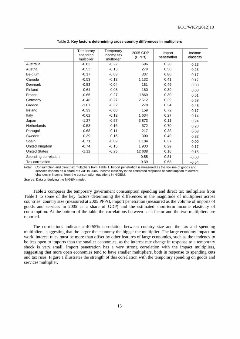
Table 2. Key factors determining cross-country differences in multipliers

Temporary spending multiplier

Temporary income tax multiplier

2005 GDP (PPPs)

Import penetration

Income elasticity

Australia -0.82 -0.22 696 0.20 0.23 Austria -0.53 -0.13 279 0.50 0.23 Belgium -0.17 -0.03 337 0.80 0.17 Canada -0.53 -0.12 1 132 0.41 0.17 Denmark -0.53 -0.04 181 0.49 0.00 Finland -0.64 -0.08 160 0.39 0.00 France -0.65 -0.27 1869 0.30 0.51 Germany -0.48 -0.27 2 512 0.39 0.68 Greece -1.07 -0.32 278 0.34 0.48 Ireland -0.33 -0.08 159 0.72 0.17 Italy -0.62 -0.12 1 634 0.27 0.14 Japan -1.27 -0.57 3 873 0.11 0.24 Netherlands -0.53 -0.16 572 0.70 0.23 Portugal -0.68 -0.11 217 0.38 0.08 Sweden -0.39 -0.16 300 0.40 0.22 Spain -0.71 -0.09 1 184 0.37 0.00 United Kingdom -0.74 -0.15 1 933 0.29 0.17 United States -1.12 -0.25 12 638 0.16 0.15 Spending correlation -0.55 0.81 -0.08 Tax correlation -0.39 0.63 -0.54

Note: Consumption and direct tax multipliers from Table 1. Import penetration is measured as the volume of goods and services imports as a share of GDP in 2005. Income elasticity is the estimated response of consumption to current changes in income, from the consumption equations in NiGEM.

Source: Data underlying the NIGEM model.

Table 2 compares the temporary government consumption spending and direct tax multipliers from Table 1 to some of the key factors determining the differences in the magnitude of multipliers across countries: country size (measured at 2005 PPPs), import penetration (measured as the volume of imports of goods and services in 2005 as a share of GDP) and the estimated short-term income elasticity of consumption. At the bottom of the table the correlations between each factor and the two multipliers are reported.

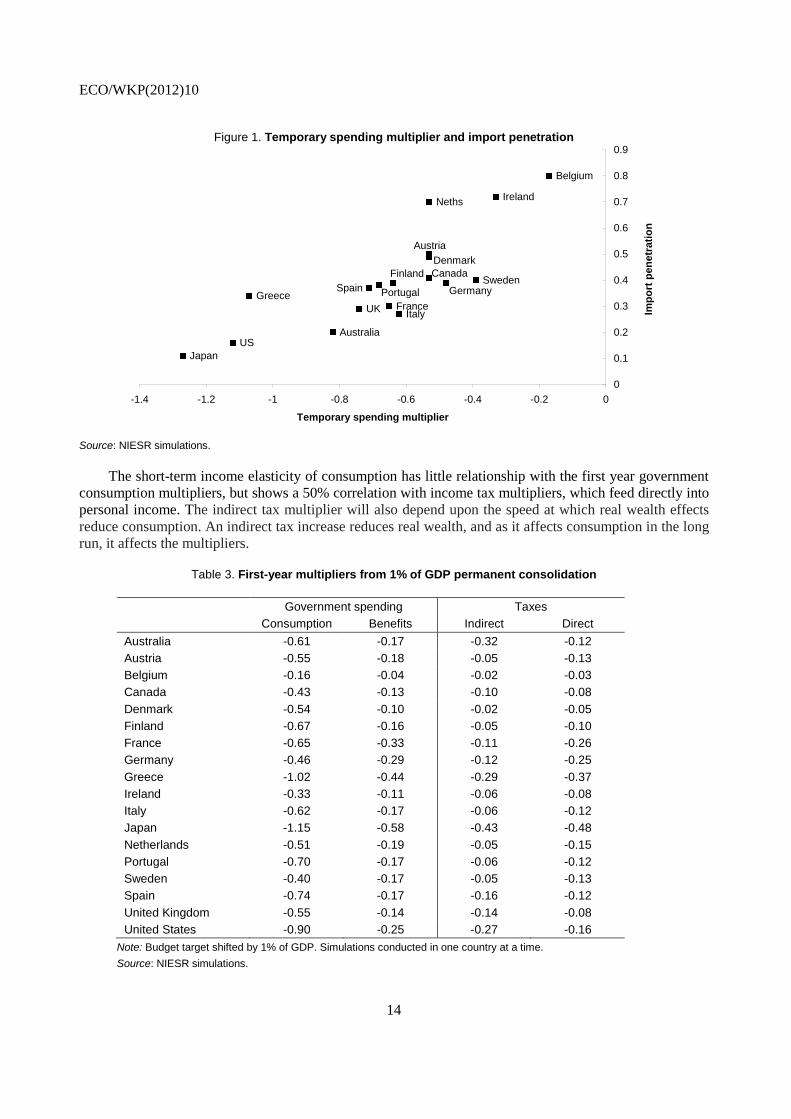
The correlations indicate a 40-55% correlation between country size and the tax and spending multipliers, suggesting that the larger the economy the bigger the multiplier. The large economy impact on world interest rates must be more than offset by other features of large economies, such as the tendency to be less open to imports than the smaller economies, as the interest rate change in response to a temporary shock is very small. Import penetration has a very strong correlation with the impact multipliers, suggesting that more open economies tend to have smaller multipliers, both in response to spending cuts and tax rises. Figure 1 illustrates the strength of this correlation with the temporary spending on goods and services multiplier.

ECO/WKP(2012)10

14

Figure 1. Temporary spending multiplier and import penetration

Source: NIESR simulations.

The short-term income elasticity of consumption has little relationship with the first year government consumption multipliers, but shows a 50% correlation with income tax multipliers, which feed directly into personal income. The indirect tax multiplier will also depend upon the speed at which real wealth effects reduce consumption. An indirect tax increase reduces real wealth, and as it affects consumption in the long run, it affects the multipliers.

Table 3. First-year multipliers from 1% of GDP permanent consolidation

Government spending Taxes Consumption Benefits Indirect Direct

Australia -0.61 -0.17 -0.32 -0.12 Austria -0.55 -0.18 -0.05 -0.13 Belgium -0.16 -0.04 -0.02 -0.03 Canada -0.43 -0.13 -0.10 -0.08 Denmark -0.54 -0.10 -0.02 -0.05 Finland -0.67 -0.16 -0.05 -0.10 France -0.65 -0.33 -0.11 -0.26 Germany -0.46 -0.29 -0.12 -0.25 Greece -1.02 -0.44 -0.29 -0.37 Ireland -0.33 -0.11 -0.06 -0.08 Italy -0.62 -0.17 -0.06 -0.12 Japan -1.15 -0.58 -0.43 -0.48 Netherlands -0.51 -0.19 -0.05 -0.15 Portugal -0.70 -0.17 -0.06 -0.12 Sweden -0.40 -0.17 -0.05 -0.13 Spain -0.74 -0.17 -0.16 -0.12 United Kingdom -0.55 -0.14 -0.14 -0.08 United States -0.90 -0.25 -0.27 -0.16

Note: Budget target shifted by 1% of GDP. Simulations conducted in one country at a time. Source: NIESR simulations.

Australia

Belgium

Ireland

Italy

Japan

Neths

Sweden

UK

US

CanadaDenmark

Finland

FranceGermanyGreece

Austria

PortugalSpain

0

0.1

0.2

0.3

0.4

0.5

0.6

0.7

0.8

0.9

-1.4 -1.2 -1 -0.8 -0.6 -0.4 -0.2 0

Temporary spending multiplier

Impo

rt p

enet

ratio

n

ECO/WKP(2012)10

15

A permanent fiscal consolidation also involves changing the budget deficit target. The reported multipliers in Table 3 are derived from the shocks applied in Table 1, but with the cut in spending or increase in taxes being permanent and also the deficit target is shifted by 1% of GDP. This changes the shape of the multiplier, as income taxes will rise in all scenarios from the second year of the simulation to cover any shortfall in the 1% of GDP consolidation, and long-term interest rates will fall by more than for a temporary consolidation. The impact of tax increases in the second year varies across shocks, depending on the degree of shortfall in the ex post budget improvement compared to the ex ante estimates.

In general, permanent multipliers should be smaller than temporary ones, as the impact of the fiscal contraction on long rates will be larger, and the fall in long rates will induce increases in asset prices and in investment.5

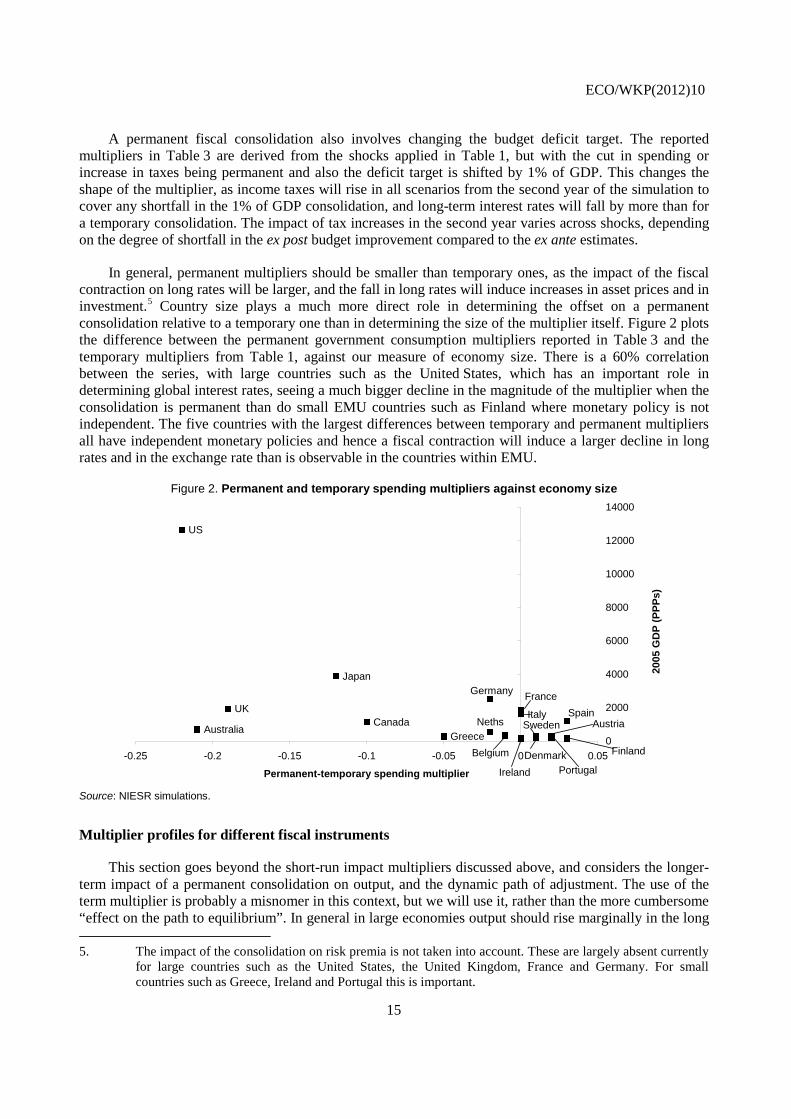
Figure 2. Permanent and temporary spending multipliers against economy size

Country size plays a much more direct role in determining the offset on a permanent consolidation relative to a temporary one than in determining the size of the multiplier itself. Figure 2 plots the difference between the permanent government consumption multipliers reported in Table 3 and the temporary multipliers from Table 1, against our measure of economy size. There is a 60% correlation between the series, with large countries such as the United States, which has an important role in determining global interest rates, seeing a much bigger decline in the magnitude of the multiplier when the consolidation is permanent than do small EMU countries such as Finland where monetary policy is not independent. The five countries with the largest differences between temporary and permanent multipliers all have independent monetary policies and hence a fiscal contraction will induce a larger decline in long rates and in the exchange rate than is observable in the countries within EMU.


Multiplier profiles for different fiscal instruments

This section goes beyond the short-run impact multipliers discussed above, and considers the longer-term impact of a permanent consolidation on output, and the dynamic path of adjustment. The use of the term multiplier is probably a misnomer in this context, but we will use it, rather than the more cumbersome “effect on the path to equilibrium”. In general in large economies output should rise marginally in the long 5. The impact of the consolidation on risk premia is not taken into account. These are largely absent currently

for large countries such as the United States, the United Kingdom, France and Germany. For small countries such as Greece, Ireland and Portugal this is important.

AustraliaCanada

Japan

UK

US

Belgium Denmark Finland

FranceGermany

Greece

Ireland

ItalyNeths Austria

Portugal

SwedenSpain

0

2000

4000

6000

8000

10000

12000

14000

-0.25 -0.2 -0.15 -0.1 -0.05 0 0.05

Permanent-temporary spending multiplier

2005

GD

P (P

PPs)

ECO/WKP(2012)10

16

run in response to a fiscal consolidation in that country alone, as real interest rates will eventually be lower. The profiles for a number of countries are reported, and each starts with the impact multipliers in Table 3.

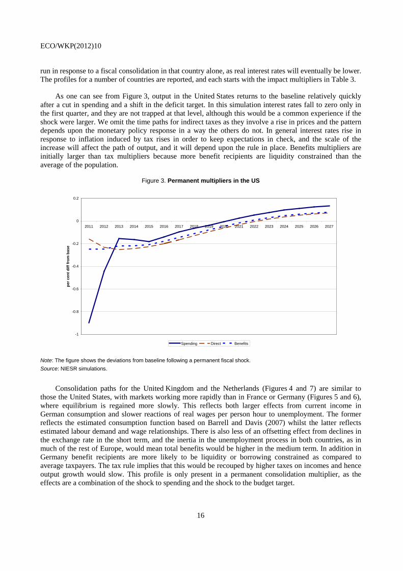
As one can see from Figure 3, output in the United States returns to the baseline relatively quickly after a cut in spending and a shift in the deficit target. In this simulation interest rates fall to zero only in the first quarter, and they are not trapped at that level, although this would be a common experience if the shock were larger. We omit the time paths for indirect taxes as they involve a rise in prices and the pattern depends upon the monetary policy response in a way the others do not. In general interest rates rise in response to inflation induced by tax rises in order to keep expectations in check, and the scale of the increase will affect the path of output, and it will depend upon the rule in place. Benefits multipliers are initially larger than tax multipliers because more benefit recipients are liquidity constrained than the average of the population.

Figure 3. Permanent multipliers in the US

Note: The figure shows the deviations from baseline following a permanent fiscal shock. Source: NIESR simulations.

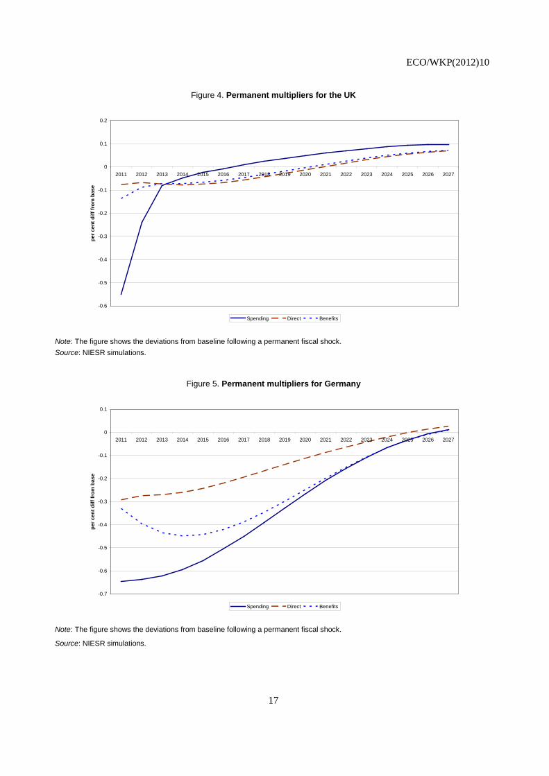
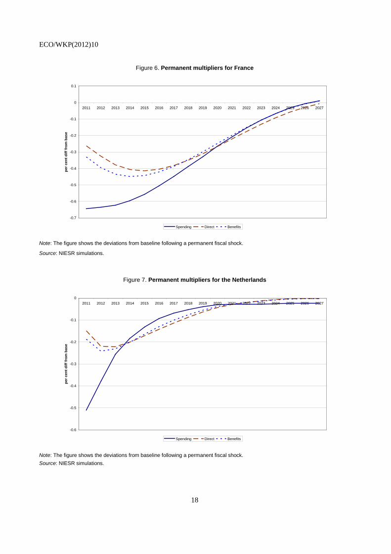
Consolidation paths for the United Kingdom and the Netherlands (Figures 4 and 7) are similar to those the United States, with markets working more rapidly than in France or Germany (Figures 5 and 6), where equilibrium is regained more slowly. This reflects both larger effects from current income in German consumption and slower reactions of real wages per person hour to unemployment. The former reflects the estimated consumption function based on Barrell and Davis (2007) whilst the latter reflects estimated labour demand and wage relationships. There is also less of an offsetting effect from declines in the exchange rate in the short term, and the inertia in the unemployment process in both countries, as in much of the rest of Europe, would mean total benefits would be higher in the medium term. In addition in Germany benefit recipients are more likely to be liquidity or borrowing constrained as compared to average taxpayers. The tax rule implies that this would be recouped by higher taxes on incomes and hence output growth would slow. This profile is only present in a permanent consolidation multiplier, as the effects are a combination of the shock to spending and the shock to the budget target.

-1

-0.8

-0.6

-0.4

-0.2

0

0.2

2011 2012 2013 2014 2015 2016 2017 2018 2019 2020 2021 2022 2023 2024 2025 2026 2027

per c

ent d

iff fr

om b

ase

Spending Direct Benefits

ECO/WKP(2012)10

17

Figure 4. Permanent multipliers for the UK


Figure 5. Permanent multipliers for Germany

Note: The figure shows the deviations from baseline following a permanent fiscal shock.


-0.6

-0.5

-0.4

-0.3

-0.2

-0.1

0

0.1

0.2

2011 2012 2013 2014 2015 2016 2017 2018 2019 2020 2021 2022 2023 2024 2025 2026 2027

per c

ent d

iff fr

om b

ase


-0.7

-0.6

-0.5

-0.4

-0.3

-0.2

-0.1

0

0.1

2011 2012 2013 2014 2015 2016 2017 2018 2019 2020 2021 2022 2023 2024 2025 2026 2027

per c

ent d

iff fr

om b

ase


ECO/WKP(2012)10

18

Figure 6. Permanent multipliers for France

Note: The figure shows the deviations from baseline following a permanent fiscal shock.


Figure 7. Permanent multipliers for the Netherlands


-0.7

-0.6

-0.5

-0.4

-0.3

-0.2

-0.1

0

0.1

2011 2012 2013 2014 2015 2016 2017 2018 2019 2020 2021 2022 2023 2024 2025 2026 2027

per c

ent d

iff fr

om b

ase


-0.6

-0.5

-0.4

-0.3

-0.2

-0.1

02011 2012 2013 2014 2015 2016 2017 2018 2019 2020 2021 2022 2023 2024 2025 2026 2027

per c

ent d

iff fr

om b

ase


ECO/WKP(2012)10

19

The long-run multipliers are based on the assumption of an exogenous labour supply. If one were to allow an endogenous response of labour supply to either a rise in the income tax rate, which may reduce incentives to enter the labour force, or a decline in the benefit rate, which may increase incentives to enter the labour force, this would result in a permanent shift in labour supply and hence potential output. The magnitude of the impact would depend on the assumed elasticity of labour supply to the tax and benefit rates.

US fiscal multipliers under different monetary policy rules

The fiscal multipliers reported in Tables 1 and 3 and illustrated in Figures 3-7 above are based on the series of assumptions detailed above. However, multipliers are not immutable, and in the next two sections the implications of some of these assumptions will be assessed, and the impact on the estimated multipliers from adopting an alternative set of assumptions reported. In this section the focus is on the choice of the monetary policy response to a fiscal consolidation. We use the United States as an example, but similar results can be expected in other large advanced economies.

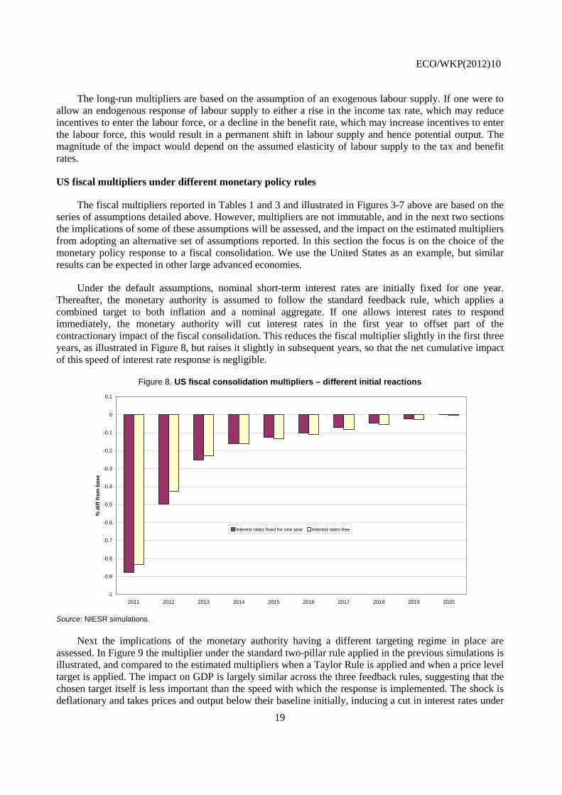
Under the default assumptions, nominal short-term interest rates are initially fixed for one year. Thereafter, the monetary authority is assumed to follow the standard feedback rule, which applies a combined target to both inflation and a nominal aggregate. If one allows interest rates to respond immediately, the monetary authority will cut interest rates in the first year to offset part of the contractionary impact of the fiscal consolidation. This reduces the fiscal multiplier slightly in the first three years, as illustrated in Figure 8, but raises it slightly in subsequent years, so that the net cumulative impact of this speed of interest rate response is negligible.

Figure 8. US fiscal consolidation multipliers – different initial reactions


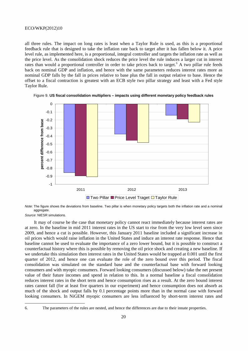
Next the implications of the monetary authority having a different targeting regime in place are assessed. In Figure 9 the multiplier under the standard two-pillar rule applied in the previous simulations is illustrated, and compared to the estimated multipliers when a Taylor Rule is applied and when a price level target is applied. The impact on GDP is largely similar across the three feedback rules, suggesting that the chosen target itself is less important than the speed with which the response is implemented. The shock is deflationary and takes prices and output below their baseline initially, inducing a cut in interest rates under

-1

-0.9

-0.8

-0.7

-0.6

-0.5

-0.4

-0.3

-0.2

-0.1

0

0.1

2011 2012 2013 2014 2015 2016 2017 2018 2019 2020

% d

iff fr

om b

ase

Interest rates fixed for one year Interest rates free

ECO/WKP(2012)10

20

all three rules. The impact on long rates is least when a Taylor Rule is used, as this is a proportional feedback rule that is designed to take the inflation rate back to target after it has fallen below it. A price level rule, as implemented here, is a proportional, integral controller and targets the inflation rate as well as the price level. As the consolidation shock reduces the price level the rule induces a larger cut in interest rates than would a proportional controller in order to take prices back to target.6

Figure 9. US fiscal consolidation multipliers – impacts using different monetary policy feedback rules

A two pillar rule feeds back on nominal GDP and inflation, and hence with the same parameters reduces interest rates more as nominal GDP falls by the fall in prices relative to base plus the fall in output relative to base. Hence the offset to a fiscal contraction is greatest with an ECB style two pillar strategy and least with a Fed style Taylor Rule.

Note: The figure shows the deviations from baseline. Two pillar is when monetary policy targets both the inflation rate and a nominal

aggregate. Source: NIESR simulations.

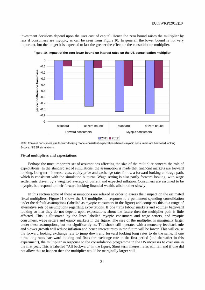
It may of course be the case that monetary policy cannot react immediately because interest rates are at zero. In the baseline in mid 2011 interest rates in the US start to rise from the very low level seen since 2009, and hence a cut is possible. However, this January 2011 baseline included a significant increase in oil prices which would raise inflation in the United States and induce an interest rate response. Hence that baseline cannot be used to evaluate the importance of a zero lower bound, but it is possible to construct a counterfactual history where this is possible by removing the oil price shock and creating a new baseline. If we undertake this simulation then interest rates in the United States would be trapped at 0.001 until the first quarter of 2012, and hence one can evaluate the role of the zero bound over this period. The fiscal consolidation was simulated on the standard base and the counterfactual base with forward looking consumers and with myopic consumers. Forward looking consumers (discussed below) take the net present value of their future incomes and spend in relation to this. In a normal baseline a fiscal consolidation reduces interest rates in the short term and hence consumption rises as a result. At the zero bound interest rates cannot fall (for at least five quarters in our experiment) and hence consumption does not absorb as much of the shock and output falls by 0.1 percentage points more than in the normal case with forward looking consumers. In NiGEM myopic consumers are less influenced by short-term interest rates and 6. The parameters of the rules are nested, and hence the differences are due to their innate properties.

-1

-0.9

-0.8

-0.7

-0.6

-0.5

-0.4

-0.3

-0.2

-0.1

0

2011 2012 2013

perc

ent d

iffer

ence

from

bas

e

Two Pillar Price Level Traget Taylor Rule

ECO/WKP(2012)10

21

investment decisions depend upon the user cost of capital. Hence the zero bound raises the multiplier by less if consumers are myopic, as can be seen from Figure 10. In general, the lower bound is not very important, but the longer it is expected to last the greater the effect on the consolidation multiplier.

Figure 10. Impact of the zero lower bound on interest rates on the US consolidation multiplier

Note: Forward consumers use forward-looking model-consistent expectation whereas myopic consumers are backward looking. Source: NIESR simulations.

Fiscal multipliers and expectations

Perhaps the most important set of assumptions affecting the size of the multiplier concern the role of expectations. In the standard set of simulations, the assumption is made that financial markets are forward looking. Long-term interest rates, equity price and exchange rates follow a forward looking arbitrage path, which is consistent with the simulation outturns. Wage setting is also partly forward looking, with wage settlements driven by a weighted average of current and expected inflation. Consumers are assumed to be myopic, but respond to their forward looking financial wealth, albeit rather slowly.

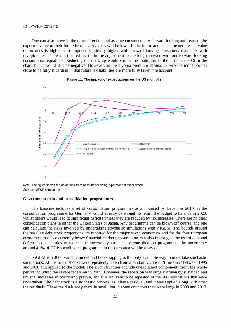
In this section some of these assumptions are relaxed in order to assess their impact on the estimated fiscal multipliers. Figure 11 shows the US multiplier in response to a permanent spending consolidation under the default assumptions (labelled as myopic consumers in the figure) and compares this to a range of alternative sets of assumptions regarding expectations. If one turns labour markets and equities backward looking so that they do not depend upon expectations about the future then the multiplier path is little affected. This is illustrated by the lines labelled myopic consumers and wage setters, and myopic consumers, wage setters and equity markets in the figure. The size of the multiplier is marginally larger under these assumptions, but not significantly so. The shock still operates with a monetary feedback rule and slower growth will reduce inflation and hence interest rates in the future will be lower. This will cause the forward looking exchange rate to jump down and forward looking long rates to do the same. If one turns long rates backward looking and fixes the exchange rate in the first period (and thereafter in this experiment), the multiplier in response to the consolidation programme in the US increases to over one in the first year. This is labelled “All backward” in the figure. Short term interest rates still fall and if one did not allow this to happen then the multiplier would be marginally larger still.

-1

-0.9

-0.8

-0.7

-0.6

-0.5

-0.4

-0.3

-0.2

-0.1

0

standard at zero bound standard at zero bound

Forward consumers Myopic consumers

per c

ent d

iffer

ence

from

bas

e

2011 2012

ECO/WKP(2012)10

22

One can also move in the other direction and assume consumers are forward looking and react to the expected value of their future incomes. As taxes will be lower in the future and hence the net present value of incomes is higher, consumption is initially higher with forward looking consumers than it is with myopic ones. There is estimated inertia in the adjustment to the long run even with our forward looking consumption equations. Reducing the mark up would shrink the multiplier further from the -0.6 in the chart, but it would still be negative. However, as the myopia premium shrinks to zero the model comes close to be fully Ricardian in that future tax liabilities are more fully taken into account.

Figure 11. The impact of expectations on the US multiplier


Government debt and consolidation programmes

The baseline includes a set of consolidation programmes as announced by December 2010, as the consolidation programme for Germany would already be enough to return the budget to balance in 2020, whilst others would lead to significant deficits unless they are reduced by tax increases. There are no clear consolidation plans in either the United States or Japan. Any programme can be blown off course, and one can calculate the risks involved by undertaking stochastic simulations with NiGEM. The bounds around the baseline debt stock projections are reported for the major seven economies and for the four European economies that face currently heavy financial market pressure. One can also investigate the use of debt and deficit feedback rules to reduce the uncertainty around any consolidation programme, the uncertainty around a 1% of GDP spending led programme in the euro area will be assessed.

NiGEM is a 3000 variable model and bootstrapping is the only available way to undertake stochastic simulations. All historical shocks were repeatedly taken from a randomly chosen ‘time slice’ between 1995 and 2010 and applied to the model. The error structures include unexplained components from the whole period including the severe recession in 2009. However, the recession was largely driven by sustained and unusual increases in borrowing premia, and it is unlikely to be repeated in the 200 replications that were undertaken. The debt stock is a stochastic process, as it has a residual, and it was applied along with other the residuals. These residuals are generally small, but in some countries they were large in 2009 and 2010.

-1.2

-1

-0.8

-0.6

-0.4

-0.2

0

0.2

0.4

2011 2012 2013 2014 2015 2016 2017 2018 2019 2020 2021

Ou

tpu

t %

dif

f fr

om

bas

elin

e

Myopic consumers All Backward

Myopic consumers, wage setters and equity markets Myopic consumers and wage setters

All Forward

ECO/WKP(2012)10

23

Estimated serial correlation in the errors is maintained, and for these variables it is not strong. The model is run with a set of residuals and the outturn is used in the next period when another time slice is applied in the next stage of the future history.

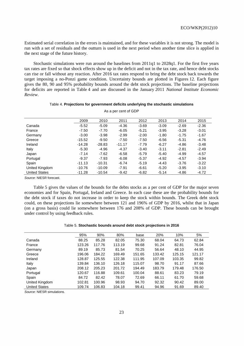
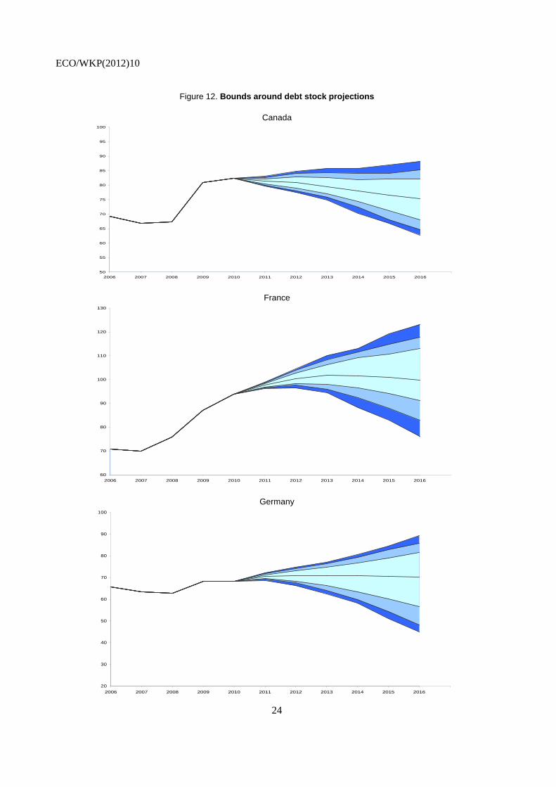
Stochastic simulations were run around the baselines from 2011q1 to 2028q1. For the first five years tax rates are fixed so that shock effects show up in the deficit and not in the tax rate, and hence debt stocks can rise or fall without any reaction. After 2016 tax rates respond to bring the debt stock back towards the target imposing a no-Ponzi game condition. Uncertainty bounds are plotted in Figures 12. Each figure gives the 80, 90 and 95% probability bounds around the debt stock projections. The baseline projections for deficits are reported in Table 4 and are discussed in the January 2011 National Institute Economic Review.

Table 4. Projections for government deficits underlying the stochastic simulations

As a per cent of GDP

2009 2010 2011 2012 2013 2014 2015 Canada -5.52 -5.09 -4.36 -3.69 -3.09 -2.69 -2.36 France -7.50 -7.70 -6.05 -5.21 -3.95 -3.28 -3.01 Germany -3.00 -3.98 -2.99 -2.00 -1.80 -1.75 -1.67 Greece -15.52 -9.50 -7.50 -7.50 -6.56 -5.31 -4.76 Ireland -14.28 -28.83 -11.17 -7.79 -6.27 -4.86 -3.48 Italy -5.30 -4.96 -4.37 -3.40 -3.11 -2.81 -2.49 Japan -7.14 -7.62 -6.58 -5.79 -5.40 -4.99 -4.57 Portugal -9.37 -7.93 -6.08 -5.37 -4.92 -4.57 -3.94 Spain -11.13 -10.31 -6.74 -5.19 -4.43 -3.76 -3.22 United Kingdom -10.76 -10.09 -7.91 -6.61 -5.20 -3.95 -3.10 United States -11.28 -10.54 -9.42 -6.82 -5.14 -4.86 -4.72

Source: NIESR forecast.

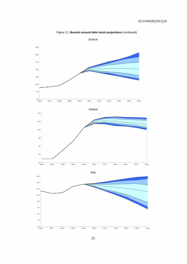
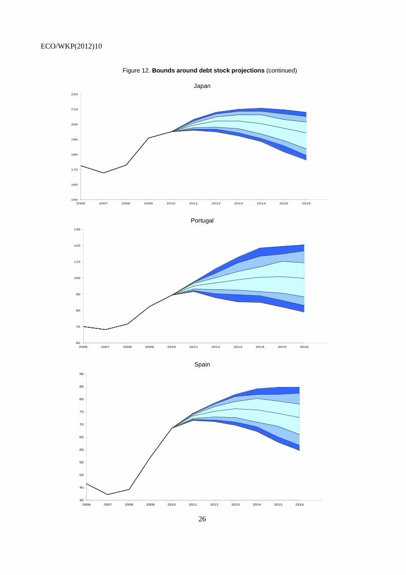
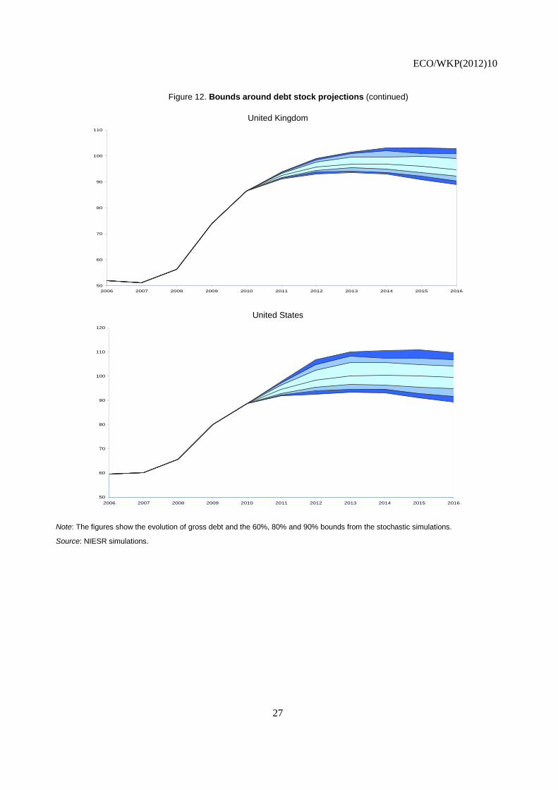
Table 5 gives the values of the bounds for the debts stocks as a per cent of GDP for the major seven economies and for Spain, Portugal, Ireland and Greece. In each case these are the probability bounds for the debt stock if taxes do not increase in order to keep the stock within bounds. The Greek debt stock could, on these projections lie somewhere between 121 and 196% of GDP by 2016, whilst that in Japan (on a gross basis) could lie somewhere between 176 and 208% of GDP. These bounds can be brought under control by using feedback rules.

Table 5. Stochastic bounds around debt stock projections in 2016

95% 90% 80% base 20% 10% 5% Canada 88.25 85.28 82.05 75.30 68.04 64.73 62.84 France 123.26 117.76 113.19 99.68 91.24 82.81 76.04 Germany 89.19 85.73 81.54 70.25 56.64 48.10 44.95 Greece 196.06 184.22 169.49 151.65 133.42 125.15 121.17 Ireland 128.87 125.55 122.38 111.95 107.09 103.35 99.82 Italy 139.84 136.10 126.18 115.07 98.70 91.17 87.66 Japan 208.12 205.23 201.72 194.49 183.79 179.48 176.50 Portugal 120.67 116.88 109.61 100.04 88.61 83.23 79.19 Spain 84.72 82.42 78.07 72.69 66.11 61.70 59.68 United Kingdom 102.81 100.96 98.93 94.70 92.32 90.42 89.00 United States 109.74 106.83 104.18 99.41 94.96 91.69 89.40


ECO/WKP(2012)10

24

Figure 12. Bounds around debt stock projections

Canada

France

Germany

50

55

60

65

70

75

80

85

90

95

100

2006 2007 2008 2009 2010 2011 2012 2013 2014 2015 2016

60

70

80

90

100

110

120

130

2006 2007 2008 2009 2010 2011 2012 2013 2014 2015 2016

20

30

40

50

60

70

80

90

100

2006 2007 2008 2009 2010 2011 2012 2013 2014 2015 2016

ECO/WKP(2012)10

25

Figure 12. Bounds around debt stock projections (continued)

Greece

Ireland

Italy

70

90

110

130

150

170

190

210

2006 2007 2008 2009 2010 2011 2012 2013 2014 2015 2016

20

40

60

80

100

120

140

2006 2007 2008 2009 2010 2011 2012 2013 2014 2015 2016

60

70

80

90

100

110

120

130

140

2006 2007 2008 2009 2010 2011 2012 2013 2014 2015 2016

ECO/WKP(2012)10

26


Japan

Portugal

Spain

150

160

170

180

190

200

210

220

2006 2007 2008 2009 2010 2011 2012 2013 2014 2015 2016

60

70

80

90

100

110

120

130

2006 2007 2008 2009 2010 2011 2012 2013 2014 2015 2016

40

45

50

55

60

65

70

75

80

85

90

2006 2007 2008 2009 2010 2011 2012 2013 2014 2015 2016

ECO/WKP(2012)10

27


United Kingdom

United States

Note: The figures show the evolution of gross debt and the 60%, 80% and 90% bounds from the stochastic simulations.


50

60

70

80

90

100

110

2006 2007 2008 2009 2010 2011 2012 2013 2014 2015 2016

50

60

70

80

90

100

110

120

2006 2007 2008 2009 2010 2011 2012 2013 2014 2015 2016

ECO/WKP(2012)10

28

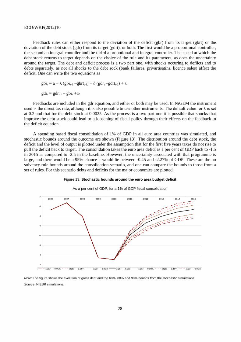
Feedback rules can either respond to the deviation of the deficit (gbr) from its target (gbrt) or the deviation of the debt stock (gdr) from its target (gdrt), or both. The first would be a proportional controller, the second an integral contoller and the thrird a propotional and integral controller. The speed at which the debt stock returns to target depends on the choice of the rule and its parameters, as does the uncertainty around the target. The debt and deficit process is a two part one, with shocks occuring to defiicts and to debts separately, as not all shocks to the debt sock (bank failures, privartisatins, licence sales) affect the deficit. One can write the two equations as

gbrt = a + λ (gbrt-1 –gbrtt-1) + δ (gdrt –gdrtt-1) + εt

gdrt = gdrt-1 – gbrt +ωt

Feedbacks are included in the gdr equation, and either or both may be used. In NiGEM the instrument used is the direct tax rate, although it is also possible to use other instruments. The default value for λ is set at 0.2 and that for the debt stock at 0.0025. As the process is a two part one it is possible that shocks that improve the debt stock could lead to a loosening of fiscal policy through their effects on the feedback in the deficit equation.

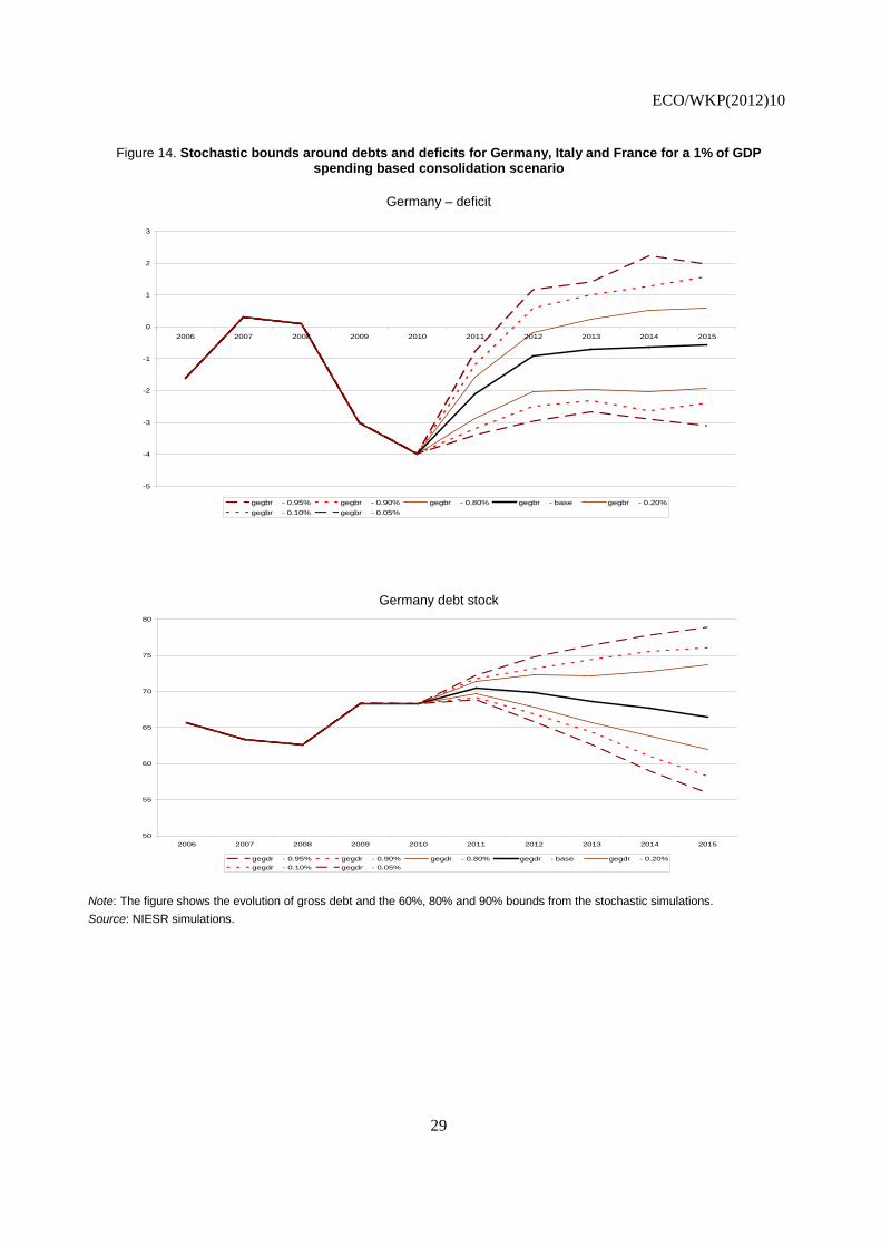
A spending based fiscal consolidation of 1% of GDP in all euro area countries was simulated, and stochastic bounds around the outcome are shown (Figure 13). The distribution around the debt stock, the deficit and the level of output is plotted under the assumption that for the first five years taxes do not rise to pull the deficit back to target. The consolidation takes the euro area defict as a per cent of GDP back to -1.5 in 2015 as compared to -2.5 in the baseline. However, the uncertainty associated with that programme is large, and there would be a 95% chance it would lie between -0.45 and -2.27% of GDP. These are the no solvency rule bounds around the consolidation scenario, and one can compare the bounds to those from a set of rules. For this scenario debts and deficits for the major economies are plotted.

Figure 13. Stochastic bounds around the euro area budget deficit

As a per cent of GDP, for a 1% of GDP fiscal consolidation

Note: The figure shows the evolution of gross debt and the 60%, 80% and 90% bounds from the stochastic simulations.


-7

-6

-5

-4

-3

-2

-1

02006 2007 2008 2009 2010 2011 2012 2013 2014 2015

elgbr - 0.95% elgbr - 0.90% elgbr - 0.80% elgbr - base elgbr - 0.20% elgbr - 0.10% elgbr - 0.05%

ECO/WKP(2012)10

29

Figure 14. Stochastic bounds around debts and deficits for Germany, Italy and France for a 1% of GDP spending based consolidation scenario

Germany – deficit

Germany debt stock

Note: The figure shows the evolution of gross debt and the 60%, 80% and 90% bounds from the stochastic simulations. Source: NIESR simulations.

-5

-4

-3

-2

-1

0

1

2

3

2006 2007 2008 2009 2010 2011 2012 2013 2014 2015

gegbr - 0.95% gegbr - 0.90% gegbr - 0.80% gegbr - base gegbr - 0.20%gegbr - 0.10% gegbr - 0.05%

50

55

60

65

70

75

80

2006 2007 2008 2009 2010 2011 2012 2013 2014 2015

gegdr - 0.95% gegdr - 0.90% gegdr - 0.80% gegdr - base gegdr - 0.20%gegdr - 0.10% gegdr - 0.05%

ECO/WKP(2012)10

30

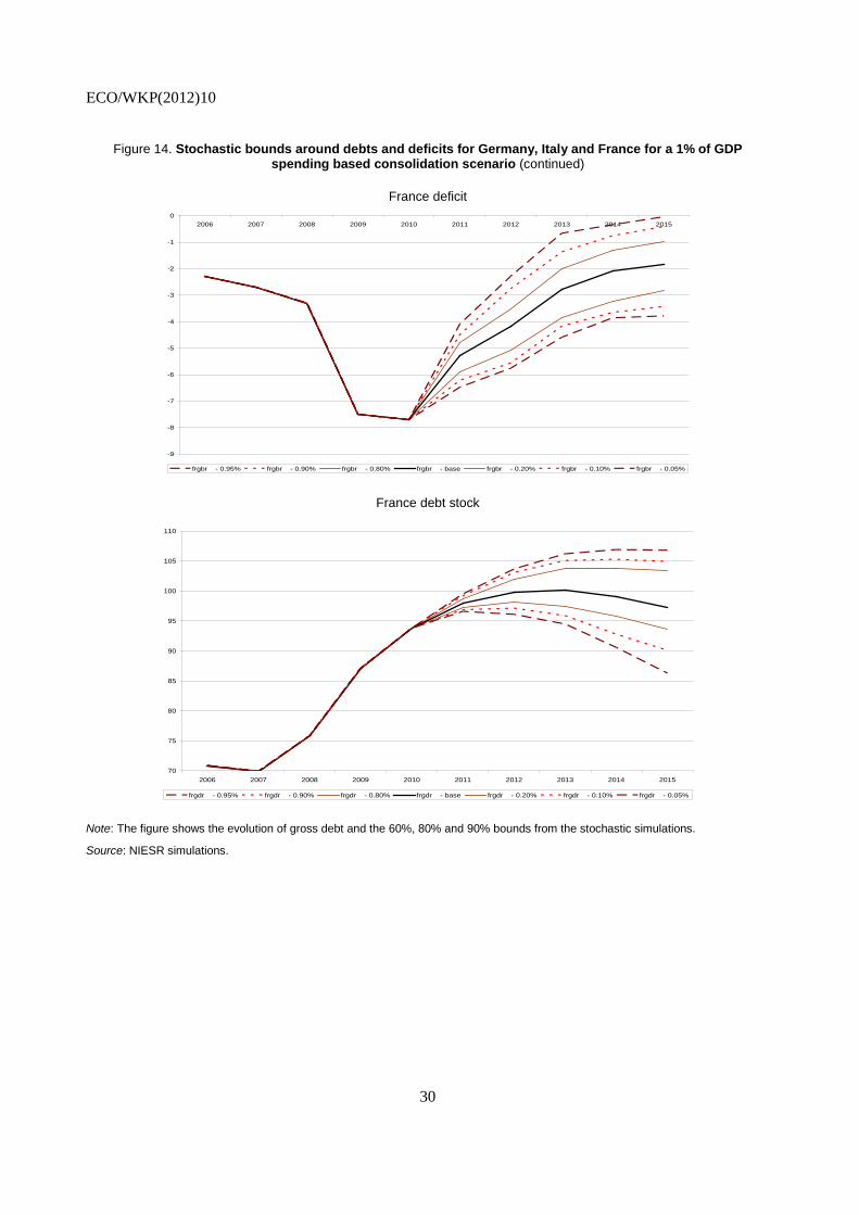
Figure 14. Stochastic bounds around debts and deficits for Germany, Italy and France for a 1% of GDP spending based consolidation scenario (continued)

France deficit

France debt stock

Note: The figure shows the evolution of gross debt and the 60%, 80% and 90% bounds from the stochastic simulations.


-9

-8

-7

-6

-5

-4

-3

-2

-1

02006 2007 2008 2009 2010 2011 2012 2013 2014 2015

frgbr - 0.95% frgbr - 0.90% frgbr - 0.80% frgbr - base frgbr - 0.20% frgbr - 0.10% frgbr - 0.05%

70

75

80

85

90

95

100

105

110

2006 2007 2008 2009 2010 2011 2012 2013 2014 2015

frgdr - 0.95% frgdr - 0.90% frgdr - 0.80% frgdr - base frgdr - 0.20% frgdr - 0.10% frgdr - 0.05%

ECO/WKP(2012)10

31

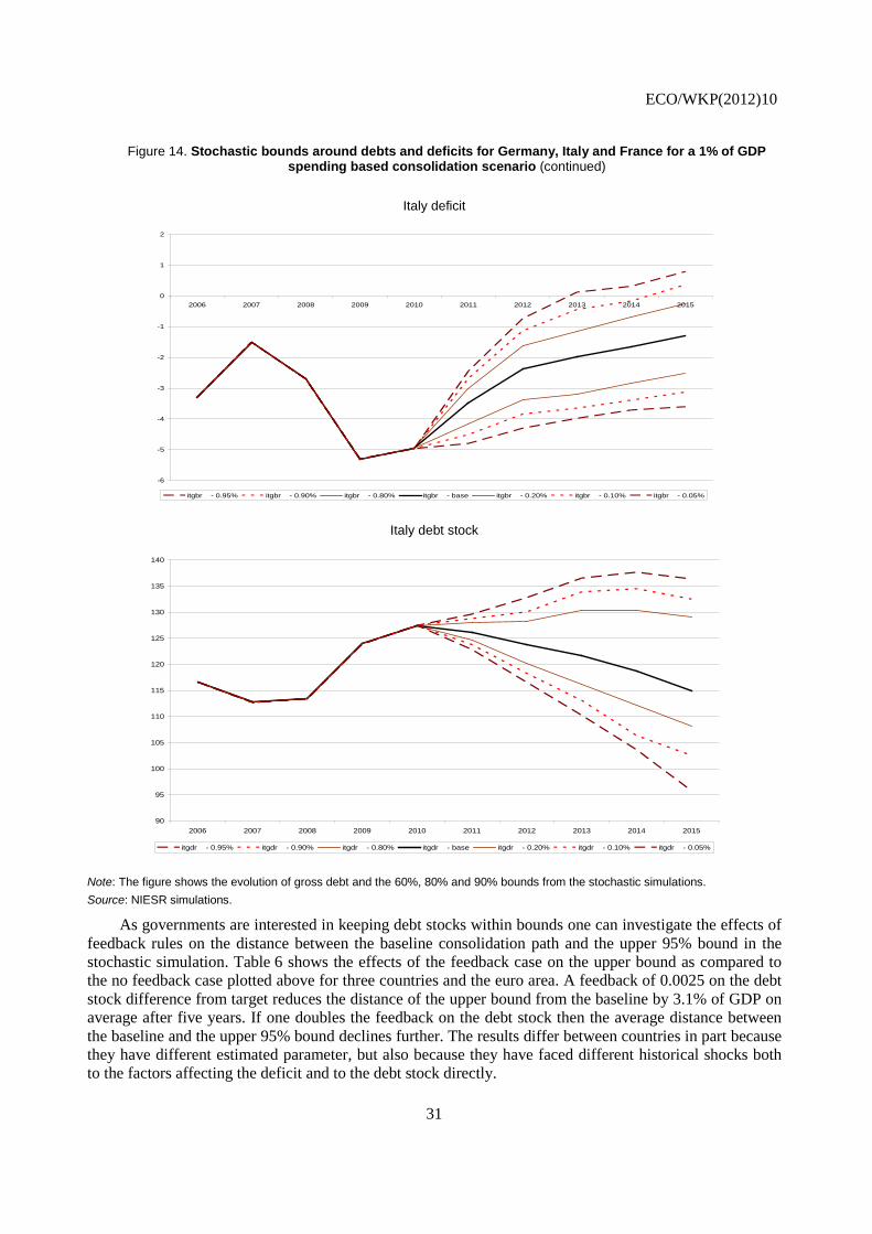
Figure 14. Stochastic bounds around debts and deficits for Germany, Italy and France for a 1% of GDP spending based consolidation scenario (continued)

Italy deficit

Italy debt stock

Note: The figure shows the evolution of gross debt and the 60%, 80% and 90% bounds from the stochastic simulations. Source: NIESR simulations.

As governments are interested in keeping debt stocks within bounds one can investigate the effects of feedback rules on the distance between the baseline consolidation path and the upper 95% bound in the stochastic simulation. Table 6 shows the effects of the feedback case on the upper bound as compared to the no feedback case plotted above for three countries and the euro area. A feedback of 0.0025 on the debt stock difference from target reduces the distance of the upper bound from the baseline by 3.1% of GDP on average after five years. If one doubles the feedback on the debt stock then the average distance between the baseline and the upper 95% bound declines further. The results differ between countries in part because they have different estimated parameter, but also because they have faced different historical shocks both to the factors affecting the deficit and to the debt stock directly.

-6

-5

-4

-3

-2

-1

0

1

2

2006 2007 2008 2009 2010 2011 2012 2013 2014 2015

itgbr - 0.95% itgbr - 0.90% itgbr - 0.80% itgbr - base itgbr - 0.20% itgbr - 0.10% itgbr - 0.05%

90

95

100

105

110

115

120

125

130

135

140

2006 2007 2008 2009 2010 2011 2012 2013 2014 2015

itgdr - 0.95% itgdr - 0.90% itgdr - 0.80% itgdr - base itgdr - 0.20% itgdr - 0.10% itgdr - 0.05%

ECO/WKP(2012)10

32

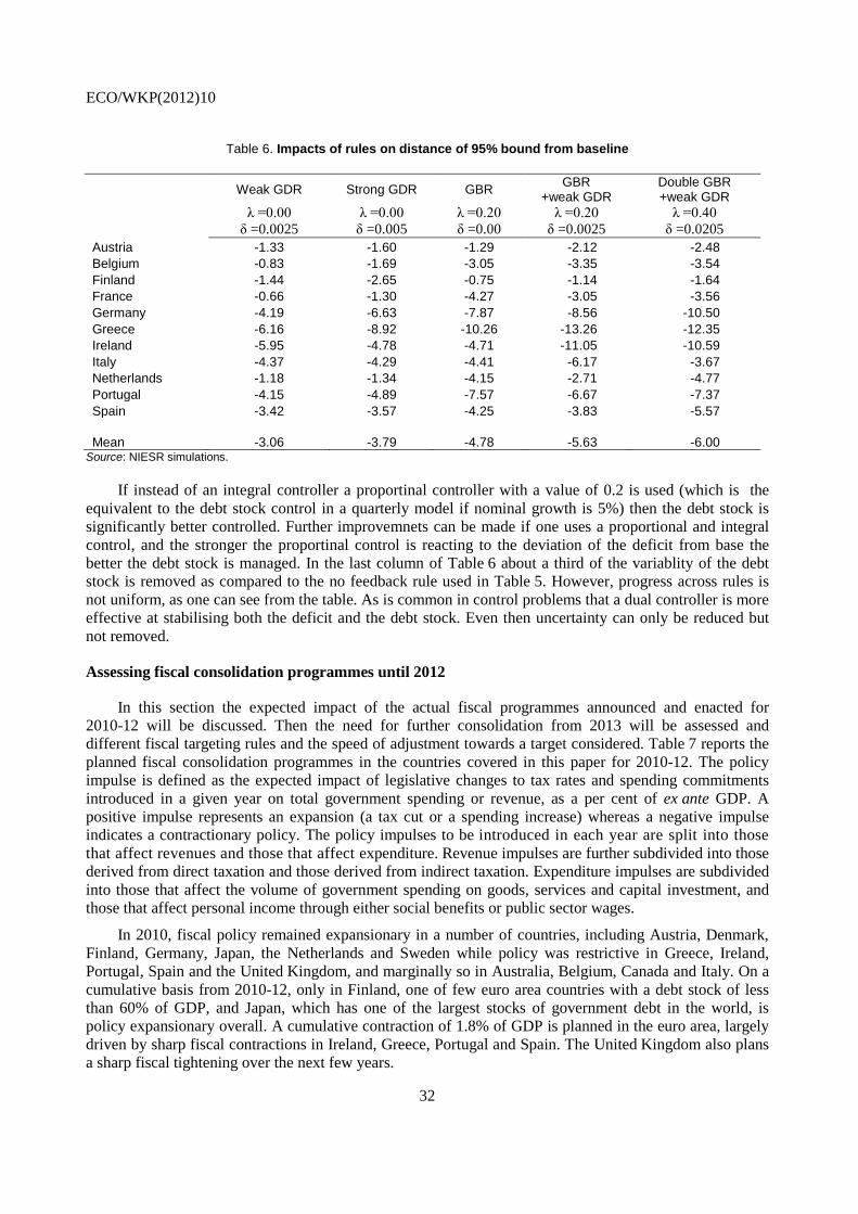
Table 6. Impacts of rules on distance of 95% bound from baseline

Weak GDR Strong GDR GBR GBR +weak GDR

Double GBR +weak GDR

λ =0.00 λ =0.00 λ =0.20 λ =0.20 λ =0.40 δ =0.0025 δ =0.005 δ =0.00 δ =0.0025 δ =0.0205

Austria -1.33 -1.60 -1.29 -2.12 -2.48 Belgium -0.83 -1.69 -3.05 -3.35 -3.54 Finland -1.44 -2.65 -0.75 -1.14 -1.64 France -0.66 -1.30 -4.27 -3.05 -3.56 Germany -4.19 -6.63 -7.87 -8.56 -10.50 Greece -6.16 -8.92 -10.26 -13.26 -12.35 Ireland -5.95 -4.78 -4.71 -11.05 -10.59 Italy -4.37 -4.29 -4.41 -6.17 -3.67 Netherlands -1.18 -1.34 -4.15 -2.71 -4.77 Portugal -4.15 -4.89 -7.57 -6.67 -7.37 Spain -3.42 -3.57 -4.25 -3.83 -5.57 Mean -3.06 -3.79 -4.78 -5.63 -6.00


If instead of an integral controller a proportinal controller with a value of 0.2 is used (which is the equivalent to the debt stock control in a quarterly model if nominal growth is 5%) then the debt stock is significantly better controlled. Further improvemnets can be made if one uses a proportional and integral control, and the stronger the proportinal control is reacting to the deviation of the deficit from base the better the debt stock is managed. In the last column of Table 6 about a third of the variablity of the debt stock is removed as compared to the no feedback rule used in Table 5. However, progress across rules is not uniform, as one can see from the table. As is common in control problems that a dual controller is more effective at stabilising both the deficit and the debt stock. Even then uncertainty can only be reduced but not removed.

Assessing fiscal consolidation programmes until 2012

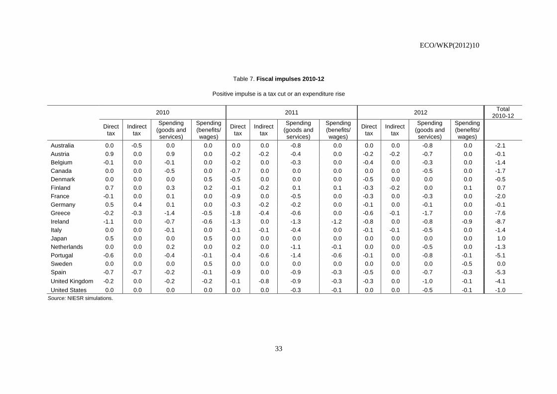
In this section the expected impact of the actual fiscal programmes announced and enacted for 2010-12 will be discussed. Then the need for further consolidation from 2013 will be assessed and different fiscal targeting rules and the speed of adjustment towards a target considered. Table 7 reports the planned fiscal consolidation programmes in the countries covered in this paper for 2010-12. The policy impulse is defined as the expected impact of legislative changes to tax rates and spending commitments introduced in a given year on total government spending or revenue, as a per cent of ex ante GDP. A positive impulse represents an expansion (a tax cut or a spending increase) whereas a negative impulse indicates a contractionary policy. The policy impulses to be introduced in each year are split into those that affect revenues and those that affect expenditure. Revenue impulses are further subdivided into those derived from direct taxation and those derived from indirect taxation. Expenditure impulses are subdivided into those that affect the volume of government spending on goods, services and capital investment, and those that affect personal income through either social benefits or public sector wages.

In 2010, fiscal policy remained expansionary in a number of countries, including Austria, Denmark, Finland, Germany, Japan, the Netherlands and Sweden while policy was restrictive in Greece, Ireland, Portugal, Spain and the United Kingdom, and marginally so in Australia, Belgium, Canada and Italy. On a cumulative basis from 2010-12, only in Finland, one of few euro area countries with a debt stock of less than 60% of GDP, and Japan, which has one of the largest stocks of government debt in the world, is policy expansionary overall. A cumulative contraction of 1.8% of GDP is planned in the euro area, largely driven by sharp fiscal contractions in Ireland, Greece, Portugal and Spain. The United Kingdom also plans a sharp fiscal tightening over the next few years.

ECO/WKP(2012)10

33

Table 7. Fiscal impulses 2010-12

Positive impulse is a tax cut or an expenditure rise

2010 2011 2012 Total 2010-12

Direct tax

Indirect tax

Spending (goods and services)

Spending (benefits/ wages)

Direct tax

Indirect tax



Direct tax

Indirect tax



Australia 0.0 -0.5 0.0 0.0 0.0 0.0 -0.8 0.0 0.0 0.0 -0.8 0.0 -2.1 Austria 0.9 0.0 0.9 0.0 -0.2 -0.2 -0.4 0.0 -0.2 -0.2 -0.7 0.0 -0.1 Belgium -0.1 0.0 -0.1 0.0 -0.2 0.0 -0.3 0.0 -0.4 0.0 -0.3 0.0 -1.4 Canada 0.0 0.0 -0.5 0.0 -0.7 0.0 0.0 0.0 0.0 0.0 -0.5 0.0 -1.7 Denmark 0.0 0.0 0.0 0.5 -0.5 0.0 0.0 0.0 -0.5 0.0 0.0 0.0 -0.5 Finland 0.7 0.0 0.3 0.2 -0.1 -0.2 0.1 0.1 -0.3 -0.2 0.0 0.1 0.7 France -0.1 0.0 0.1 0.0 -0.9 0.0 -0.5 0.0 -0.3 0.0 -0.3 0.0 -2.0 Germany 0.5 0.4 0.1 0.0 -0.3 -0.2 -0.2 0.0 -0.1 0.0 -0.1 0.0 -0.1 Greece -0.2 -0.3 -1.4 -0.5 -1.8 -0.4 -0.6 0.0 -0.6 -0.1 -1.7 0.0 -7.6 Ireland -1.1 0.0 -0.7 -0.6 -1.3 0.0 -1.3 -1.2 -0.8 0.0 -0.8 -0.9 -8.7 Italy 0.0 0.0 -0.1 0.0 -0.1 -0.1 -0.4 0.0 -0.1 -0.1 -0.5 0.0 -1.4 Japan 0.5 0.0 0.0 0.5 0.0 0.0 0.0 0.0 0.0 0.0 0.0 0.0 1.0 Netherlands 0.0 0.0 0.2 0.0 0.2 0.0 -1.1 -0.1 0.0 0.0 -0.5 0.0 -1.3 Portugal -0.6 0.0 -0.4 -0.1 -0.4 -0.6 -1.4 -0.6 -0.1 0.0 -0.8 -0.1 -5.1 Sweden 0.0 0.0 0.0 0.5 0.0 0.0 0.0 0.0 0.0 0.0 0.0 -0.5 0.0 Spain -0.7 -0.7 -0.2 -0.1 -0.9 0.0 -0.9 -0.3 -0.5 0.0 -0.7 -0.3 -5.3 United Kingdom -0.2 0.0 -0.2 -0.2 -0.1 -0.8 -0.9 -0.3 -0.3 0.0 -1.0 -0.1 -4.1 United States 0.0 0.0 0.0 0.0 0.0 0.0 -0.3 -0.1 0.0 0.0 -0.5 -0.1 -1.0


ECO/WKP(2012)10

34

A series of simulations are run to assess the impact of the planned consolidation packages on output, unemployment and the deficit in each country. The underlying assumptions of the model simulation include the following: financial markets (long-term interest rates, exchange rates and equity prices) exhibit forward-looking behaviour, consumers exhibit myopic behaviour and all consolidation measures are assumed to be permanent. Interest rates are assumed to follow the two-pillar rule and an interest rate response from the first year of the simulation is allowed. These are essentially the same assumptions underlying the permanent multipliers discussed above, with the exception of lifting the restriction on the monetary policy response in the first year. As was discussed above, this slightly reduces the impact multiplier in the first year of the simulation. The results of consolidation on a unilateral basis are compared to joint consolidations in all countries at the same time.

Figure 15 illustrates the expected impact on GDP, the unemployment rate and the fiscal balance relative to a baseline scenario with no change in the prevailing policy of 2009. These results are based on single country scenarios. Below the difference between unilateral consolidation measures and joint consolidation will be compared. The estimates suggest that fiscal tightening reduced output in Greece by 2½ per cent in 2010, with the cumulative impact on GDP expected to rise to -6½ per cent by 2012, raising the unemployment rate by nearly 2 percentage points. While the cumulative improvement in the fiscal balance in Ireland is expected to be slightly higher than in Greece, the impact on output and unemployment is smaller, reflecting the small multiplier in Ireland. Output in Spain, Portugal, the United Kingdom and Ireland is expected to be 1½ – 3 per cent below the baseline by 2012 as a result of the fiscal programmes. The impacts are smaller elsewhere.

Having considered each fiscal package on a unilateral basis, we then run a simulation with all packages introduced simultaneously. In general, we would expect negative spillovers from fiscal contractions abroad, and output to be lower in the joint scenario than in the unilateral scenarios. This is partially offset, especially in the smaller economies in the Euro Area, by the bigger impact of the joint action on ECB interest rate setting and more significant depreciation of the exchange rate.

Figure 16 illustrates the difference in the level of GDP in 2012 in each country in the joint scenario compared to the unilateral scenarios. In some cases, joint consolidation has a positive effect on output, reflecting the sensitivity of net trade to the exchange rate and relative price movements as well as the short-term sensitivity of demand to the real interest rate. The latter is particularly important in the United States and Japan. If the price elasticity of imports is high relative to that of exports, imports fall relative to exports when domestic prices are restrained, which in the very open economies of Belgium, Ireland and Austria may actually raise the level of GDP in the short term.

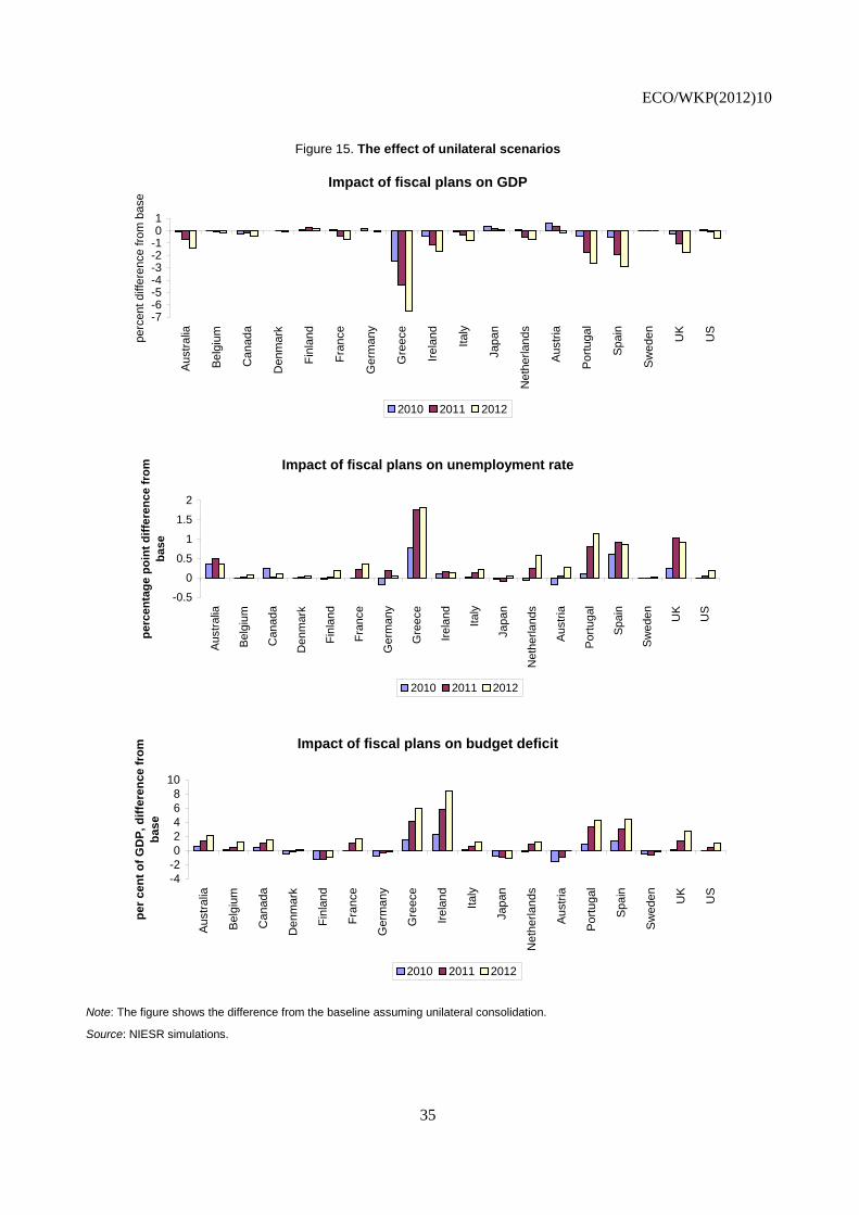
ECO/WKP(2012)10

35

Figure 15. The effect of unilateral scenarios

Note: The figure shows the difference from the baseline assuming unilateral consolidation.


Impact of fiscal plans on GDP

-7-6-5-4-3-2-101

Aust

ralia

Belg

ium

Can

ada

Den

mar

k

Finl

and

Fran

ce

Ger

man

y

Gre

ece

Irela

nd

Italy

Japa

n

Net

herla

nds

Aust

ria

Portu

gal

Spai

n

Swed

en UK

US

perc

ent d

iffer

ence

from

bas

e

2010 2011 2012

Impact of fiscal plans on unemployment rate

-0.5

0

0.5

1

1.5

2

Aus

tralia

Bel

gium

Can

ada

Den

mar

k

Finl

and

Fran

ce

Ger

man

y

Gre

ece

Irela

nd

Italy

Japa

n

Net

herla

nds

Aus

tria

Por

tuga

l

Spa

in

Sw

eden UK

US

perc

enta

ge p

oint

diff

eren

ce fr

om

base

2010 2011 2012

Impact of fiscal plans on budget deficit

-4-202468

10

Aus

tralia

Bel

gium

Can

ada

Den

mar

k

Finl

and

Fran

ce

Ger

man

y

Gre

ece

Irela

nd

Italy

Japa

n

Net

herla

nds

Aus

tria

Por

tuga

l

Spa

in

Sw

eden UK

US

per c

ent o

f GD

P, d

iffer

ence

from

ba

se

2010 2011 2012

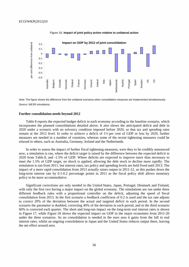
ECO/WKP(2012)10

36

Figure 16. Impact of joint policy action relative to unilateral action

Note: The figure shows the difference from the unilateral scenarios when consolidation measures are implemented simultaneously.


Further consolidation needs beyond 2012

Table 8 reports the expected budget deficit in each economy according to the baseline scenario, which incorporates the planned consolidations detailed above. It also shows the anticipated deficit and debt in 2020 under a scenario with no solvency condition imposed before 2020, so that tax and spending rates remain at the 2012 level. In order to achieve a deficit of 1½ per cent of GDP or less by 2020, further measures are needed in a number of countries, whereas some of the recent tightening measures could be relaxed in others, such as Australia, Germany, Ireland and the Netherlands.

In order to assess the impact of further fiscal tightening measures, were they to be credibly announced now, a simulation is run, where the deficit target is raised by the difference between the expected deficit in 2020 from Table 8, and -1.5% of GDP. Where deficits are expected to improve more than necessary to meet the 1.5% of GDP target, no shock is applied, allowing the debt stock to decline more rapidly. The simulation is run from 2011, but interest rates, tax policy and spending levels are held fixed until 2013. The impact of a more rapid consolidation from 2013 actually raises output in 2011-12, as this pushes down the long-term interest rate by 0.1-0.2 percentage points in 2011 as the fiscal policy shift allows monetary policy to be more accommodative.

Significant corrections are only needed in the United States, Japan, Portugal, Denmark and Finland, with only the first two having a major impact on the global economy. The simulations are run under three different feedback rules with a proportional controller on the deficit, adjusting the speed of fiscal consolidation from 2013. In the first scenario a feedback coefficient of 0.2 is used and the tax rate adjusts to correct 20% of the deviation between the actual and targeted deficit in each period. In the second scenario the parameter is doubled, correcting 40% of the deviation in each period, and in the third scenario 60% is corrected each quarter. The short and long-run impact on the long-term real interest rates is shown in Figure 17, while Figure 18 shows the expected impact on GDP in the major economies from 2011-20 under the three scenarios. As no consolidation is needed in the euro area it gains from the fall in real interest rates, whilst an ongoing consolidation in Japan and the United States reduces output there, leaving the net effect around zero.

Impact on GDP by 2012 of joint consolidation

-0.5

-0.4

-0.3

-0.2

-0.1

0

0.1

0.2A

ustra

lia

Bel

gium

Can

ada

Den

mar

k

Finl

and

Fran

ce

Ger

man

y

Gre

ece

Irela

nd

Italy

Japa

n

Net

herla

nds

Aus

tria

Por

tuga

l

Spa

in

Sw

eden UK

US

per c

ent d

iffer

ence

from

uni

late

ral

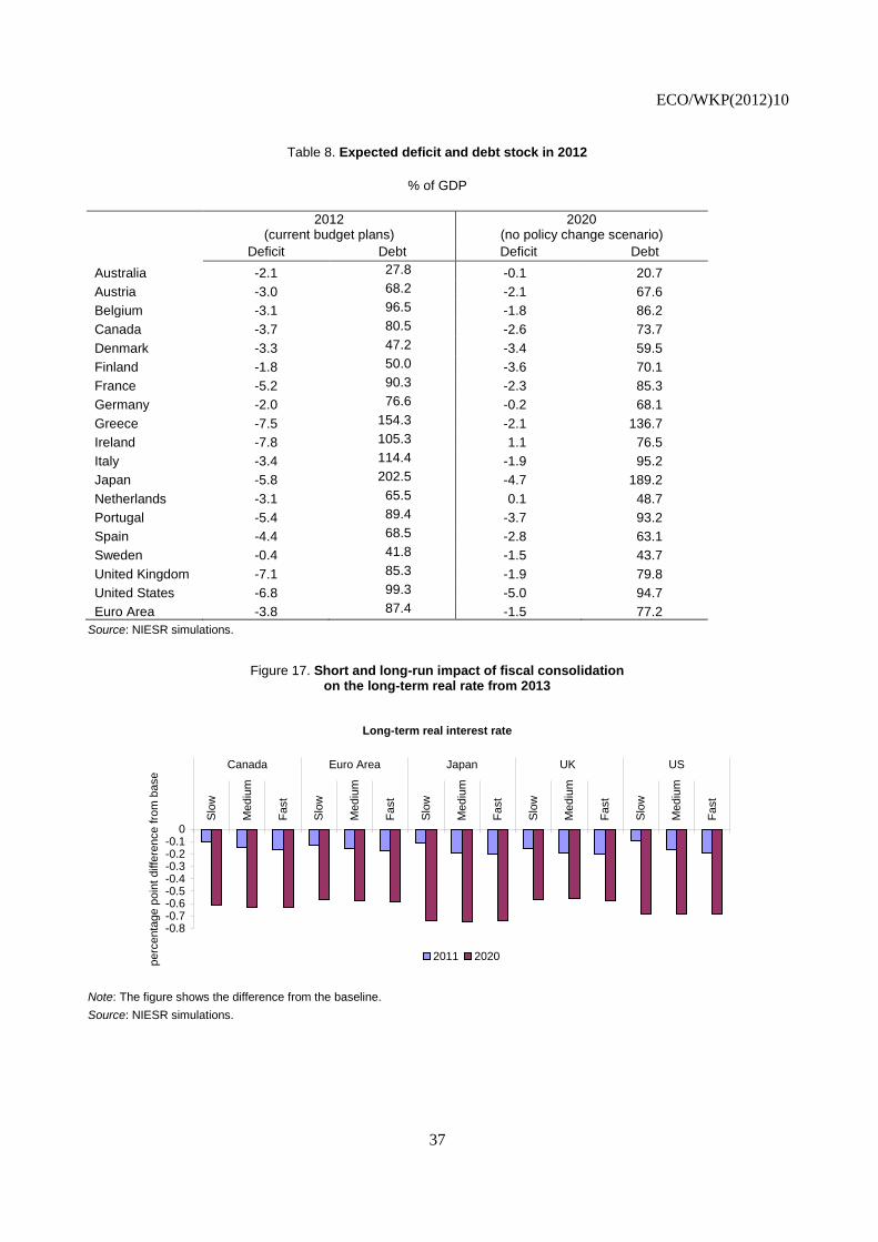
ECO/WKP(2012)10

37

Table 8. Expected deficit and debt stock in 2012

% of GDP

2012

(current budget plans) 2020

(no policy change scenario) Deficit Debt Deficit Debt

Australia -2.1 27.8 -0.1 20.7 Austria -3.0 68.2 -2.1 67.6 Belgium -3.1 96.5 -1.8 86.2 Canada -3.7 80.5 -2.6 73.7 Denmark -3.3 47.2 -3.4 59.5 Finland -1.8 50.0 -3.6 70.1 France -5.2 90.3 -2.3 85.3 Germany -2.0 76.6 -0.2 68.1 Greece -7.5 154.3 -2.1 136.7 Ireland -7.8 105.3 1.1 76.5 Italy -3.4 114.4 -1.9 95.2 Japan -5.8 202.5 -4.7 189.2 Netherlands -3.1 65.5 0.1 48.7 Portugal -5.4 89.4 -3.7 93.2 Spain -4.4 68.5 -2.8 63.1 Sweden -0.4 41.8 -1.5 43.7 United Kingdom -7.1 85.3 -1.9 79.8 United States -6.8 99.3 -5.0 94.7 Euro Area -3.8 87.4 -1.5 77.2


Figure 17. Short and long-run impact of fiscal consolidation on the long-term real rate from 2013

Note: The figure shows the difference from the baseline. Source: NIESR simulations.

Long-term real interest rate

-0.8-0.7-0.6-0.5-0.4-0.3-0.2-0.1

0

Slow

Med

ium

Fast

Slow

Med

ium

Fast

Slow

Med

ium

Fast

Slow

Med

ium

Fast

Slow

Med

ium

Fast

Canada Euro Area Japan UK US

perc

enta

ge p

oint

diff

eren

ce fr

om b

ase

2011 2020

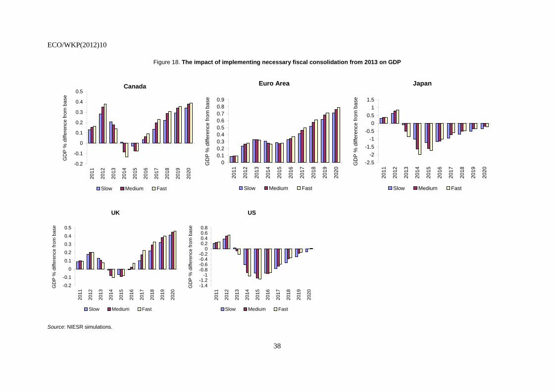
ECO/WKP(2012)10

38

Figure 18. The impact of implementing necessary fiscal consolidation from 2013 on GDP


Canada

-0.2

-0.1

0

0.1

0.2

0.3

0.4

0.520

11

2012

2013

2014

2015

2016

2017

2018

2019

2020

GD

P %

diff

eren

ce fr

om b

ase

Slow Medium Fast

Euro Area

00.10.20.30.40.50.60.70.80.9

2011

2012

2013

2014

2015

2016

2017

2018

2019

2020

GD

P %

diff

eren

ce fr

om b

ase

Slow Medium Fast

Japan

-2.5-2

-1.5-1

-0.50

0.51

1.5

2011

2012

2013

2014

2015

2016

2017

2018

2019

2020

GD

P %

diff

eren

ce fr

om b

ase

Slow Medium Fast

UK

-0.2-0.1

00.1

0.20.30.40.5

2011

2012

2013

2014

2015

2016

2017

2018

2019

2020

GD

P %

diff

eren

ce fr

om b

ase

Slow Medium Fast

US

-1.4-1.2

-1-0.8-0.6-0.4-0.2

00.20.40.60.8

2011

2012

2013

2014

2015

2016

2017

2018

2019

2020

GD

P %

diff

eren

ce fr

om b

ase

Slow Medium Fast

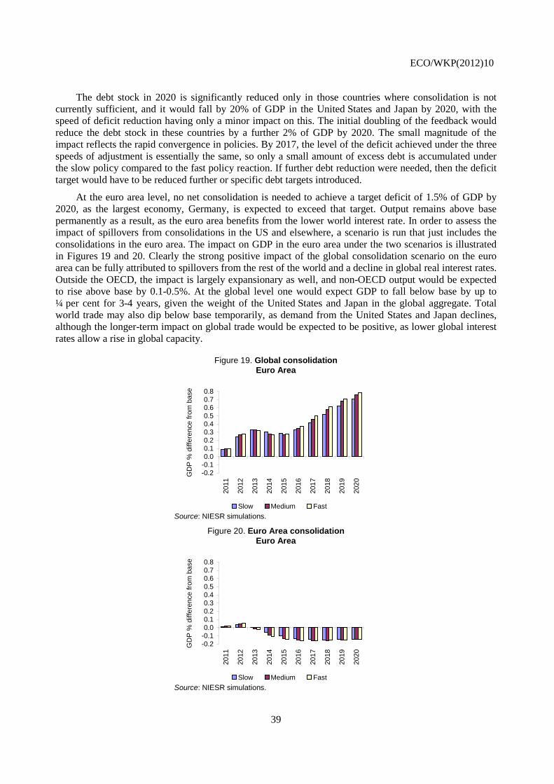
ECO/WKP(2012)10

39

The debt stock in 2020 is significantly reduced only in those countries where consolidation is not currently sufficient, and it would fall by 20% of GDP in the United States and Japan by 2020, with the speed of deficit reduction having only a minor impact on this. The initial doubling of the feedback would reduce the debt stock in these countries by a further 2% of GDP by 2020. The small magnitude of the impact reflects the rapid convergence in policies. By 2017, the level of the deficit achieved under the three speeds of adjustment is essentially the same, so only a small amount of excess debt is accumulated under the slow policy compared to the fast policy reaction. If further debt reduction were needed, then the deficit target would have to be reduced further or specific debt targets introduced.

At the euro area level, no net consolidation is needed to achieve a target deficit of 1.5% of GDP by 2020, as the largest economy, Germany, is expected to exceed that target. Output remains above base permanently as a result, as the euro area benefits from the lower world interest rate. In order to assess the impact of spillovers from consolidations in the US and elsewhere, a scenario is run that just includes the consolidations in the euro area. The impact on GDP in the euro area under the two scenarios is illustrated in Figures 19 and 20. Clearly the strong positive impact of the global consolidation scenario on the euro area can be fully attributed to spillovers from the rest of the world and a decline in global real interest rates. Outside the OECD, the impact is largely expansionary as well, and non-OECD output would be expected to rise above base by 0.1-0.5%. At the global level one would expect GDP to fall below base by up to ¼ per cent for 3-4 years, given the weight of the United States and Japan in the global aggregate. Total world trade may also dip below base temporarily, as demand from the United States and Japan declines, although the longer-term impact on global trade would be expected to be positive, as lower global interest rates allow a rise in global capacity.

Figure 19. Global consolidation


Figure 20. Euro Area consolidation


Euro Area

-0.2-0.10.00.10.20.30.40.50.60.70.8

2011

2012

2013

2014

2015

2016

2017

2018

2019

2020

GD

P %

diff

eren

ce fr

om b

ase

Slow Medium Fast

Euro Area

-0.2-0.10.00.10.20.30.40.50.60.70.8

2011

2012

2013

2014

2015

2016

2017

2018

2019

2020

GD

P %

diff

eren

ce fr

om b

ase

Slow Medium Fast

ECO/WKP(2012)10

40

Conclusion

In general in most countries fiscal policy multipliers are small, but are negative when fiscal policy is tightened. Tighter fiscal policy reduces growth in the short run in almost all circumstances, but a lower debt stock reduces pressures on real interest rates and hence in the longer term can raise sustainable output. This effect is larger for larger countries, and there are noticeable spillovers through real interest rates from policies in the United States (or from the euro area as a whole). If fiscal policy were to be noticeably tightened in the United States and Japan, as it should be, this would boost activity in the euro area as lower long-term real interest rates may well stimulate demand. The need to reduce government debt stocks cannot be denied, but their evolution is very uncertain. The bounds around any consolidation programme can be reduced by setting up automatic feedbacks that raise taxes in response to overshoots on targets for debts and deficits, but the uncertainty bounds cannot be shrunk to zero. In general targeting the debt stock and the deficit is more effective than targeting either alone as both are subject to shocks that make them deviate from target.

Bibliography

Al-Eyd, A. and R. Barrell (2005), “Estimating Tax and Benefit Multipliers in Europe”, Economic Modelling, Vol. 22.

Barrell, R. and E.P. Davis (2007), “Financial Liberalisation, Consumption and Wealth Effects in Seven OECD Countries”, Scottish Journal of Political Economy, Vol. 54, No. 2.

Barrell, R. and K. Dury (2003), “Asymmetric Labour Markets in a Converging Europe: Do Differences Matter?”, National Institute Economic Review, No. 183.

Barrell, R., A.I. Hurst and J. Mitchell (2007), “Uncertainty Bounds for Cyclically-Adjusted Budget Balances”, in: M. Larch and L.N. Martins (eds), Fiscal Indicators, European Commission, Brussels.

Barrell, R, D. Holland and A.I. Hurst (2007), “Correcting US Imbalances”, NIESR Discussion Paper, No. 290.

Barrell, R., S.G. Hall and A.I. Hurst (2006), “Evaluating Policy Feedback Rules Using the Joint Density Function of a Stochastic Model”, Economics Letters, Vol. 93, No. 1.

Barrell, R., T. Fic and I. Liadze (2009), “Fiscal Policy Effectiveness in the Banking Crisis”, National Institute Economic Review, No. 207.

Harrison, R. et al. (2005), The Bank of England Quarterly Model, Bank of England, London.

ECO/WKP(2012)10

41

WORKING PAPERS

The full series of Economics Department Working Papers can be consulted at www.oecd.org/eco/workingpapers/

932. Fiscal consolidation Part 1. How much is needed and how to reduce debt to a prudent level? (January 2012) by Douglas Sutherland, Peter Hoeller and Rossana Merola 931. Less income inequality and more growth – Are they compatible?

Part 8. The drivers of labour income inequality – A review of the recent literature (January 2012) by Rafal Kierzenkowski and Isabell Koske 930. Less income inequality and more growth – Are they compatible?

Part 7. The drivers of labour earnings inequality – An analysis based on conditional and unconditional quantile regressions

(January 2012) by Jean-Marc Fournier and Isabell Koske 929. Less income inequality and more growth – Are they compatible?

Part 6. The distribution of wealth (January 2012) by Kaja Bonesmo Fredriksen 928. Less income inequality and more growth – Are they compatible?

Part 5. Poverty in OECD countries (January 2012) by Mauro Pisu 927. Less income inequality and more growth – Are they compatible?

Part 4. Top incomes (January 2012) by Peter Hoeller 926. Less income inequality and more growth – Are they compatible?

Part 3. Income redistribution via taxes and transfers across OECD countries (January 2012) by Isabelle Joumard, Mauro Pisu and Debbie Bloch 925. Less income inequality and more growth – Are they compatible?

Part 2. The distribution of labour income (January 2012) by Isabell Koske, Jean-Marc Fournier and Isabelle Wanner 924. Less income inequality and more growth – Are they compatible?

Part 1. Mapping income inequality across the OECD (January 2012) by Peter Hoeller, Isabelle Joumard, Mauro Pisu and Debbie Bloch 923. Current issues in managing government debt and assets (December 2011) by Eckhard Wurzel and Lukasz Rawdanowicz 922. Public spending efficiency in the Czech Republic: fiscal policy framework and the main spending

areas of pensions and healthcare (December 2011) by Zuzana Smidova 921. Exploring determinants of subjective wellbeing in OECD countries – evidence from the World

Value Survey (December 2011) by Sarah Fleche, Conal Smith and Piritta Sorsa

http://www.oecd.org/eco/working_papers/�

ECO/WKP(2012)10

42

920. Russia: progress in structural reform and framework conditions (December 2011) by Yana Vaziakova, Geoff Barnard and Tatiana Lysenko 919. Explaining the interest-rate-growth differential underlying government debt dynamics (December 2011) by David Turner and Francesca Spinelli 918. Reassessing the NAIRUs after the crisis (December 2011) by Stéphanie Guichard and Elena Rusticelli 917. Employment protection legislation and plant-level productivity in India (December 2011) by Sean Dougherty, Verónica Frisancho Robles and Kala Krishna 916. Systemically important banks and capital regulation challenge (December 2011) by Patrick Slovik 915. Improving educational outcomes in Slovenia (December 2011) by Mehmet Eris 914. Addressing challenges in the energy sector in Israel (December 2011) by Philip Hemmings 913. Issues in private sector finance in Israel (December 2011) by Philip Hemmings 912. How to improve the economic policy framework for the housing market in Israel (December 2011) by Philip Hemmings 911. Fiscal Prospects and Reforms in India (December 2011) by Richard Herd, Sam Hill and Vincent Koen 910. Structural reforms to reduce unemployment and restore competitiveness in Ireland (December 2011) by Álvaro Pina 909. Getting back on track: restoring fiscal sustainability in Ireland (December 2011) by David Haugh

908. A welfare analysis of climate change mitigation policies (November 2011) by Alain de Serres and Fabrice Murtin 907. Overcoming the banking crisis in Ireland (November 2011) by Muge Adalet McGowan 906. Macroeconomic and structural policies to further stabilise the Mexican economy (November 2011) by Cyrille Schwellnus 905. Reaping the benefits of a transition to greener growth in Slovakia (November 2011) by Caroline Klein

Documents

Consolidations Fiscal Multipliers and Fiscal Fiscal ......ECO/WKP(2012)10 2 ABSTRACT/RESUMÉ Fiscal consolidation Part 2. Fiscal multipliers and fiscal consolidations This paper looks