Embed Size (px)
Citation preview

B U C H A R E S T U N I V E R S I T Y O F E C O N O M I C S T U D I E S
D O C T O R A L S C H O O L O F F I N A N C E A N D B A N K I N G
The Evolution of Fiscal Multipliers
during the Global Financial Crisis. The
Case of Romania
București
2015
Coordinator: Prof. Univ. Dr. Moisă Altăr
MSc Student: Marin Cristina Georgiana

CONTENTS
Motivation and objectives
Literature Review
Econometric Methodology, Data and
Results
Conclusions and Areas for Further
Research
References

Motivation
The economic crisis that started in 2008-2009 determined
governments and central banks to focus on the role of fiscal policy.
Fiscal policy is a tool for macroeconomic stability. Lately, public debates
concentrated on fiscal consolidation strategies and mostly on short term
results.
European countries have faced high levels of public debt. The crisis met
a new phase, where the initial problems of private sector insolvencies
shed over the public sector.
The traditional monetary policy transmission mechanism lost its
capacity to encourage private consumption. Furthermore, many
countries reached their zero lower bound on interest rate, with no room
to reduce it.
This paper completes the research about fiscal policy efficiency in
emerging countries.

Objectives
Calculating fiscal multipliers for government spending
and revenues in Romania
SVAR Model with two identification schemes (recursive
approach and Blanchard-Perotti approach)
Checking for robustness and implementing alternative
models
Decomposition of fiscal variables in their constitutive elements
Introduction of new variables in the model
Explaining the results through describing the key factors
that determine the size of the fiscal multipliers in
Romania

Fiscal multipliers
Represent the ratio of a change in output to an exogenous change in
the fiscal deficit with respect to their respective baselines
(Spilimbergo et al., 2009).
There are several definition that are of interest:
𝑇ℎ𝑒 𝑖𝑚𝑝𝑎𝑐𝑡 𝑚𝑢𝑙𝑡𝑖𝑝𝑙𝑖𝑒𝑟 = ∆𝑌(𝑡)
∆𝑍(𝑡)
𝑇ℎ𝑒 𝑝𝑒𝑎𝑘 𝑚𝑢𝑙𝑡𝑖𝑝𝑙𝑖𝑒𝑟 𝑜𝑣𝑒𝑟 𝑎 𝑡𝑖𝑚𝑒 ℎ𝑜𝑟𝑖𝑧𝑜𝑛 𝑁
= max𝑁
∆𝑌(𝑡 + 𝑁)
∆𝑍(𝑡)
𝑇ℎ𝑒 𝑐𝑢𝑚𝑢𝑙𝑎𝑡𝑖𝑣𝑒 𝑚𝑢𝑙𝑡𝑖𝑝𝑙𝑖𝑒𝑟 𝑎𝑡 𝑎 𝑡𝑖𝑚𝑒 ℎ𝑜𝑟𝑖𝑧𝑜𝑛 𝑁 = ∆𝑌(𝑡 + 𝑗𝑁𝑗=0 )
∆𝑍(𝑡 + 𝑗)𝑁𝑗=0
Fiscal policy is transmitted through a complex mechanism of
institutional and human elements. Government’s measures to
stimulate economic growth are conditioned by private agents’
behavior, anticipations and reactions.

Factors of influence
Ilzetzki, Mendoza and Végh (2011), Batini, Eyraud
and Weber (2014) describe the key factors of the size of
fiscal multipliers:
Trade openness degree
Exchange rate regime
Indebtedness
Size of automatic stabilizers
Public finances management and administration
State of the business cycle
Degree of monetary accommodation to fiscal shocks

CONTENTS
Motivation
Objectives
Literature Review
Econometric Methodology, Data and Results
Conclusions and Areas for Further Research
References

Literature Review
Linear VAR models
The recursive approach – Fatás and Mihov (2001)
The structural VAR approach (SVAR) – Blanchard and Perotti (2002) and
Perotti (2004)
The sign restriction approach – Uhlig (2005), Mountford and Uhlig (2010)
and Caldara and Kamps (2008)
The narrative approach – Ramey and Shapiro (1998), Perotti (2007) and
Caldara and Kamps (2008)
Non-linear VAR models
Smooth Transition VAR models – Auerbach and Gorodnichenko (2010),
Batini, Callegari and Melina (2012)
Threshold VAR models – Baum and Koester (2011), Fazzari et al. (2012)
Time Varying Parameter VAR models – Karagyozova-Markova et al. (2013)
DSGE models – Sims and Wolff (2014)

Fiscal multipliers in emerging economies
Authors Sample
(quarterly data)
Government spending Government revenue Identification
strategy Short
term
Medium
term Short term
Medium
term
Ilzetzki,
Mendoza and
Végh (2011)
24 developing
countries of the
world
(1960s-2000s)
(-0.2; 0.3) 0.2 - - Panel VAR
Crespo
Cuaresma,
Eller and
Mehrotra
(2011)
Czech Republic
Hungary
Poland
(1995:1 – 2009:4)
Slovakia
Slovenia
(1996:1 – 2009:4)
-
0.01
-
-0.01
-0.01
-0.04
0.01
-0.02
0.00
-0.01
-
-
-
-0.02
0.01
0.03
-0.01
0.02
-0.1
0.02
Blanchard-
Perotti
Karagyozova-
Markova,
Deyanov and
Iliev (2013)
Bulgaria
(1999:1 – 2011:3)
(0.03; 0.17)
(0.01; 0.41)
(0.15; 0.3)
(0.48; 0.7)
(0.87; 0.92)
(0.18; 0.40)
(0; 0.91)
(-0.19; 0.3)
-
(1.02; 1.48)
(-0.21; 0.43)
-
Cholesky
decomposition,
Blanchard-
Perotti and
TVP-VAR
Petrović,
Arsić and
Nojković
(2014)
10 European
emerging countries
(1999:1 – 2012:3)
(0.2; 0.58) 0.2 -0.4 0 Blanchard-
Perotti

CONTENTS
Motivation
Objectives
Literature Review
Econometric Methodology, Data and Results
Conclusions and Areas for Further Research
References

Econometric Methodology
Variable and
notation
Description and
calculation Unit Source Transformation
Government
spending
(g)
Government spending
= Intermediate consumption +
Compensation of employees +
Gross fixed capial formation Log millions units of
domestic currency Eurostat
The variables were
deflated using the GDP
deflator (2005=100) and
seasonally adjusted
using Tramo Seats
method in Eviews. The
first difference was
applied in order to
ensure stationarity
Net government
revenue
(t)
Net government revenue =
direct taxes + indirect taxes +
social contributions– subsidies
– social benefits
Real GDP
(y)
Chain linked volumes
(2005=100), log millions
units of domestic
currency, seasonally
adjusted series
Eurostat First difference in order
to achieve stationarity
Inflation rate
(p)
Quarterly modification of
prices, calculated based on the
Consumer Price Index
%
National
Institute of
Statistic
Short term
interest rate
(i)
3 months interbank offered
rate (ROBOR 3M) % per annum
National Bank
of Romania
First difference in order
to achieve stationarity
Data description
Romanian quarterly data, 2000Q1 – 2014Q4

Structural form of the VAR model:
A0 Xt = A(L) Xt-1 + B εt
A0 = (m x m) matrix of contemporaneous effects
Xt = vector of endogenous variables, (gt yt pt tt it)’
A(L) = describes the impact of lagged effects (L-th order lag polynomial matrix )
B = (m x m) structural form parameter matrix
εt = vector of structural shocks
E (εt) = 0, E (εt εt ’) = Σε = I, E (εt εs’) = 0 , ∀ t≠s
Reduced form model:
Xt = A0-1A(L) Xt-1 + A0
-1 Bεt = C(L) Xt-1 + ut ,
ut = A0-1 Bεt or A0 ut = Bεt
ut = vector of reduced form residuals:
E (ut) = 0, E (ut ut’) = Σu , E (ut us’) = 0 , ∀ t≠s
The informational criteria Schwarz and Hannan-Quinn suggest using a VAR(1)
and Akaike criterion – a VAR(4) model. In small sample, the latter leads to
better results, so 4 lags will be used, similar to Blanchard and Perotti (2002).
VAR Model Specification

Allows for the identification of the fiscal shocks through a Cholesky decomposition
of the variance-covariance matrix of errors (Lütkepohl, 2005).
It can be written:
Σu = P P’
by defining a diagonal matrix D that has the same main diagonal as P and by specifying:
A0-1 = P D-1 and Σε = DD’
It gives:
Σu = A0-1 Σε (A0
-1)’.
The system can be expressed as:
The sequence of the variables requires certain assumptions:
government spending does not react contemporaneously to any shock in other variables;
output is affected within a quarter only by the government spending innovations;
revenues do not react within a period to a interest rate modification, but are influenced by the
shocks in spending and output, as a result of changing their respective macroeconomic base.
The recursive approach

Blanchard - Perotti approach
Reduced VAR model:
Xt = C(L) Xt-1 + ut
Matrix A0 is no longer lower triangular and B is no longer an identity
matrix.
The system can be written:
In order to achieve identification, restrictions in contemporaneous responses in the system are imposed:
αgt = αtg = 0 –> Public spending and revenue do not influence each other contemporaneously.
αgy = 0 –> Government spendings are net of transfers, so acyclic.
αji = 0, ∀ j –> The interest rate does not influence within a quarter any of the variables.
αyp=0 –> Real GDP does not respond to inflation.
βgt =0 –> Spending decision comes first.

Exogenous elasticities
Government revenues
PIT CIT Indirect
taxes
Social
contributions Subsidies
Social
benefits
Total
elasticity
Output elasticity 0.20 1.59 0.94 0.18 0 -0.20 1.20
Price elasticity 0.35 0 0 -0.10 -1 -1 0.84
Share in total
government
revenue (%)
29.89 9.75 77.31 63.18 -6.43 -73.70
Intermediate
consumption
Gross fixed
capital formation
Compensation
of employees
Total
elasticity
Price elasticity 0 0 -1 -0.45
Share in total
government spending
(%)
32.65 21.76 45.59
Government spendings
Source: Price, Dang și Guillemette (2014), Perotti (2004) and own calculations
The aggregate values are calculated as weghted averages of the sub-elasticities of each component, using their shares in total revenues or spending.

Results Baseline model : Fiscal multipliers have small dimensions.
0,00
0,10
0,20
0,30
0,40
Cumulative fiscal multipliers – the recursive identification approach
G (Chol.)
T (Chol.)
-0,10
0,00
0,10
0,20
0,30
0,40
Cumulative fiscal multipliers – the Blanchard-Perotti identification approach
G (BP)
T (BP)
Results for the expenditure multiplier are in line with Ilzetzki et al. (2011).
After 5 quarters, the revenue multiplier overpasses the one of spending, but in the long run they have similar dimensions (0.18).
Peak values: G: 0.35 ; T: 0.23
Spending multiplier has a similar
value as in the recursive approach.
Revenue multiplier is smaller and
negative at impact (long run
value:0.13).
Results are in line with the
Keynesian theory (higher spending
multipliers)
Peak values: G: 0.36; T: 0.18 Identification
approach
Fiscal
multiplier
Quarters after the shock
1 4 8 12 16
Cholesky
decomposition
G 0.04 0.29 0.22 0.18 0.18
T 0.02 0.15 0.20 0.20 0.18
Blanchard-
Perotti
G 0.04 0.29 0.22 0.18 0.20
T -0.02 0.10 0.16 0.15 0.13

Key factors of the size of fiscal multipliers
Trade openness degree
0%20%40%60%80%
100%120%140%160%
Trade openness in European countries (% of
GDP, average 2000-2014)
Source: Eurostat, European Commission
Public debt and budgetar deficit
0
10
20
30
40
50
0
2
4
6
8
10
2000 2001 2002 2003 2004 2005 2006 2007 2008 2009 2010 2011 2012 2013 2014
Public debt and budget deficit in Romania
(% of GDP)
Public debt-to-GDP ratio (right axis) Budget deficit
Flexible exchange rate regime
Romania is a small open
economy, which reduces the
fiscal multipliers.
The public debt-to-GDP ratio is
relatively small, but fiscal policy is not
predictabe and trustworthy. Between
2009 and 2013 there were over 130
changes of the Fiscal Code.
Budgetary equilibrium suffers in the
absence of a coherent long term fiscal
strategy.

Public finances management and administration
0
1
2
3
4
5
Public investment spending (% of
GDP, average 2000-2014)
0
1
2
3
4
5
6
7
Infrastructure score (2014)
Small size of automatic
stabilizers
Source: Eurostat, World Economic Forum, The Global
Competitiveness Report 2014-2015
00,10,20,30,40,50,60,7
Automatic stabilizers in European
countries
Source: European Commission (2014)
High allocation of investment
spending, but weak infrastructure
–> inefficient expenditures
They are measured as the semi-
elasticity of budget balance and
their level acts inversely on fiscal
multipliers.

a. VAR(1) vs VAR (4)
Lower and flat-shaped multipliers in a VAR(1) model –> VAR(4) better
captures the system dynamics.
When the output elasticity of taxes is set to 0.8, the multiplier is smaller.
In the other cases, the results do not change significantly.
-0,10
0,00
0,10
0,20
0,30
0,40
1Q
2Q
3Q
4Q
5Q
6Q
7Q
8Q
9Q
10
Q
11
Q
12
Q
13
Q
14
Q
15
Q
16
Q
Fiscal multipliers in VAR(1) and
VAR(4)
G (VAR(4))
T (VAR(4))
G (VAR(1))
T (VAR(1))
Robustness Check
b. Different elasticities of
taxes with respect to
output and prices
(following Crespo
Cuaresma et al., 2011,
αty = 0.8 and αtp=0.5)
c. Different price
elasticity of
government spending
(αgp from -1 to 0)
d. Taxes decision comes
first: βtg = 0

Cumulative fiscal multipliers of government spending and revenue
components
Component Quarters after the shock Peak
multiplier 1 4 8 12 16
Intermediate
consumption 0 0.17 0.12 0.15 0.14 0.44 (5Q)
Gross fixed capital
formation 0 0.08 0.06 0.05 0.05 0.08 (3Q)
Compensation of
employees 0.11 0.30 0.23 0.23 0.22 0.33 (3Q)
Direct taxes 0 0.12 0.08 0.08 0.09 0.13 (3Q)
Indirect taxes -0.01 0.23 0.11 0.14 0.12 0.38 (5Q)
Social contributions 0.03 0.42 0.34 0.30 0.31 0.45 (3Q)
Extended models
Public spending for employees compensation have the biggest impact on output,
given their share in total expenditures (45.6%).
Social contributions revenues are the second largest component of revenue, but
they are higher than the VAT component of indirect taxes (average of 9% compared
to 7.9%)

Cumulative multipliers of private consumption and of investment
(following Heppke-Falk et al., 2006)
Endogenous variables Cumulative multiplier
Peak value Impact First year Long term
Government spending, private
consumption, inflation, government
revenue, interest rate
G 0.07 0.33 0.25 0.39 (3Q)
T -0.08 0.04 0.08 0.11 (8Q)
Government spending, investment,
inflation, government revenue, interest
rate
G 0.14 1.00 0.65 1.10 (3Q)
T -0.48 0.49 0.71 0.96 (8Q)
Extended models (2)
Impulse responses to a positive
government spending shock
Impulse responses to a positive
government revenue shock
Neo-Keynesian theory: private
consumption is crowded in by
government spending and
crowded out by taxation.
Neoclassical theory: a positive
shock in public spending leads to
a raise in investment.
The effects of spending and
revenue have opposite signs on
impact.
-.02
-.01
.00
.01
.02
.03
.04
1 2 3 4 5 6 7 8 9 10 11 12 13 14 15 16
Private consumption
-.04
-.02
.00
.02
.04
.06
.08
1 2 3 4 5 6 7 8 9 10 11 12 13 14 15 16
Investment
-.02
-.01
.00
.01
.02
.03
.04
1 2 3 4 5 6 7 8 9 10 11 12 13 14 15 16
Private consumption
-.04
-.02
.00
.02
.04
.06
.08
1 2 3 4 5 6 7 8 9 10 11 12 13 14 15 16
Investment

Following Ilzetzki, Mendoza and Végh (2011) and Petrović et al. (2014)
VAR Model
Quarters after the shock Peak
multiplier Impact First year Long
term
Baseline model with Blanchard-
Perotti identification
G 0.04 0.29 0.20 0.36 (3Q)
T -0.02 0.10 0.15 0.18 (6Q)
Exogenous variable: public debt
(Ilzetzki, Mendoza and Végh, 2011)
G 0.03 0.25 0.16 0.36 (3Q)
T -0.06 0.08 0.09 0.14 (6Q)
Endogenous variables: g, y, current
account, ∆ reer (Petrović et al., 2014) G 0.01 0.12 0.07 0.15 (3Q)
Endogenous variables: g, t, y;
Exogenous variables: current
account, ∆ reer, output gap of EU-15
(Petrović et al., 2014)
G 0.02 0.16 0.05 0.25 (3Q)
T -0.04 0.05 0.08 0.10 (3Q)
Extended models (3)
Fiscal multipliers tend to have a smaller value when other variables are included in the model, because they bring additional information about macroeconomical factors (exchange rate regime, public finances sustainability) that diminish the impact of fiscal stimuli.
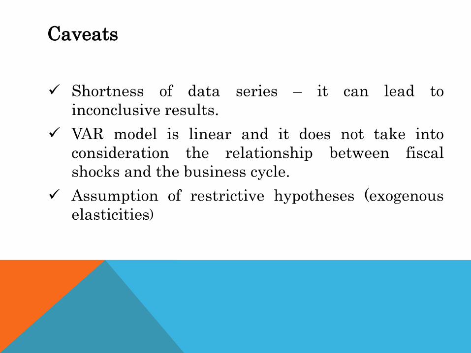
Caveats
Shortness of data series – it can lead to
inconclusive results.
VAR model is linear and it does not take into
consideration the relationship between fiscal
shocks and the business cycle.
Assumption of restrictive hypotheses (exogenous
elasticities)

CONTENTS
Motivation
Objectives
Literature Review
Econometric Methodology, Data and Results
Conclusions and Areas for Further Research
References

Conclusions
The fiscal multipliers obtained in Romania for period 2000-2014 are in line with
other studies in the literature:
first-year spending multipliers: 0.01 to 0.36
first-year revenue multipliers: – 0.06 to 0.15.
Their dimension is reduced compared to advanced economies, Romania being a
small open country. The flexible exchange rate regime lowers this value, while the
automatic stabilizers and public debt levels acts on it in the opposite way. The
collective lack of confidence of agents makes it hard for the government revival
actions to take effect.
Among the fiscal variables components, changes in compensations of public sector
employees and in social contributions spread the most efficiently in the economy.
Private consumption reacts more slightly than investment to a fiscal shock, fact
that reinforces the idea of a need for reorganization of public expenditures, in the
sense of directing them into investment plans that could sustain the long term
economic development.
Raising the question of public debt influence leads to smaller values for the
multipliers.
The large palette of values in the literature can be explained by a plurality of
political, financial and economic factors and by the absence of a commonly accepted
econometric methodology to identify exogenous fiscal shocks.

Areas for Further Research
Non-linear fiscal multiplier analyze: applying a Threshold
VAR, a Time-Varying Parameter VAR or a Regime-Switching
VAR, to highlight the effects of business cycles over fiscal
policy efficiency in Romania.
Transmission of foreign fiscal shocks (from an important
trading partner) in domestic output, considering that
Romania is an emerging country that can support many
influences.
Avoiding data series lenght restrictions by implementing
models calibrated with explicit macroeconomic basis (DSGE
models)

CONTENTS
Motivation
Objectives
Literature Review
Econometric Methodology, Data and Results
Conclusions and Areas for Further Research
References
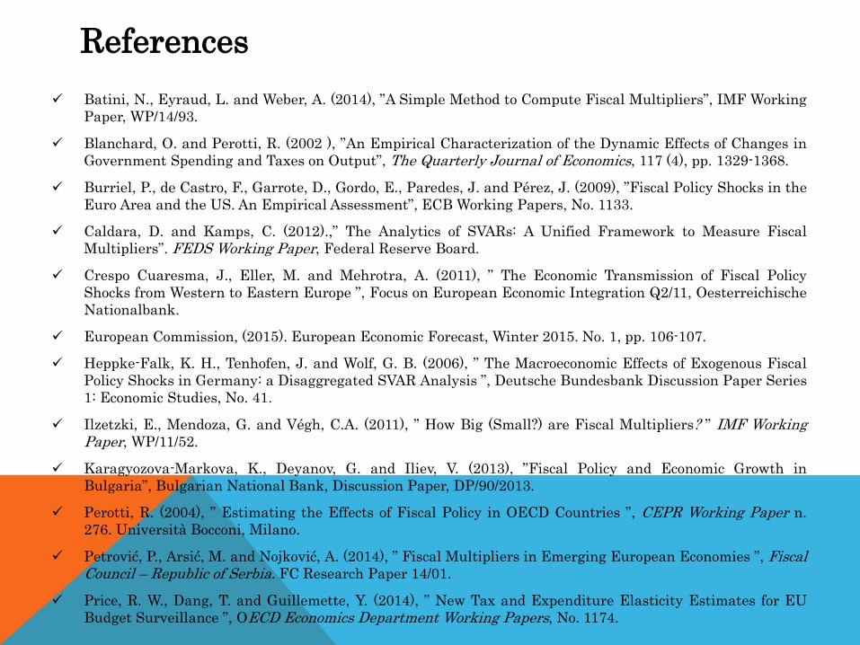
References
Batini, N., Eyraud, L. and Weber, A. (2014), ”A Simple Method to Compute Fiscal Multipliers”, IMF Working
Paper, WP/14/93.
Blanchard, O. and Perotti, R. (2002 ), ”An Empirical Characterization of the Dynamic Effects of Changes in
Government Spending and Taxes on Output”, The Quarterly Journal of Economics, 117 (4), pp. 1329-1368.
Burriel, P., de Castro, F., Garrote, D., Gordo, E., Paredes, J. and Pérez, J. (2009), ”Fiscal Policy Shocks in the
Euro Area and the US. An Empirical Assessment”, ECB Working Papers, No. 1133.
Caldara, D. and Kamps, C. (2012).,” The Analytics of SVARs: A Unified Framework to Measure Fiscal
Multipliers”. FEDS Working Paper, Federal Reserve Board.
Crespo Cuaresma, J., Eller, M. and Mehrotra, A. (2011), ” The Economic Transmission of Fiscal Policy
Shocks from Western to Eastern Europe ”, Focus on European Economic Integration Q2/11, Oesterreichische
Nationalbank.
European Commission, (2015). European Economic Forecast, Winter 2015. No. 1, pp. 106-107.
Heppke-Falk, K. H., Tenhofen, J. and Wolf, G. B. (2006), ” The Macroeconomic Effects of Exogenous Fiscal
Policy Shocks in Germany: a Disaggregated SVAR Analysis ”, Deutsche Bundesbank Discussion Paper Series
1: Economic Studies, No. 41.
Ilzetzki, E., Mendoza, G. and Végh, C.A. (2011), ” How Big (Small?) are Fiscal Multipliers? ” IMF Working Paper, WP/11/52.
Karagyozova-Markova, K., Deyanov, G. and Iliev, V. (2013), ”Fiscal Policy and Economic Growth in
Bulgaria”, Bulgarian National Bank, Discussion Paper, DP/90/2013.
Perotti, R. (2004), ” Estimating the Effects of Fiscal Policy in OECD Countries ”, CEPR Working Paper n.
276. Università Bocconi, Milano.
Petrović, P., Arsić, M. and Nojković, A. (2014), ” Fiscal Multipliers in Emerging European Economies ”, Fiscal Council – Republic of Serbia. FC Research Paper 14/01.
Price, R. W., Dang, T. and Guillemette, Y. (2014), ” New Tax and Expenditure Elasticity Estimates for EU
Budget Surveillance ”, OECD Economics Department Working Papers, No. 1174.

THANK YOU FOR YOUR ATTENTION!