CONSOLIDATING PYTHON UTILITIES TO FACILITATE ROOT LOCUS DESIGN

HONORS THESIS

Presented to the Honors College of Texas State University in Partial Fulfillment of the Requirements

for Graduation in the Honors College

by

Zachary Angel Rangel

San Marcos, Texas December 2019

CONSOLIDATING PYTHON UTILITIES TO FACILITATE ROOT LOCUS DESIGN

by

Zachary Angel Rangel

Thesis Supervisor: ________________________________ Cecil Richard Compeau, Ph.D. Department of Electrical Engineering

Second Reader: __________________________________ William Albert Stapleton, Ph.D. Department of Electrical Engineering

Approved: ____________________________________ Heather C. Galloway, Ph.D. Dean, Honors College

Acknowledgments

Many thanks to Dr. Compeau and Dr. Stapleton for their contributions to both this

project and my overall education and career in electrical engineering. I would not be an

engineer without their help.

My gratitude is also extended to the great sources of motivation in my life who

supported me and galvanized my work ethic, even in the times where I would have much

preferred to sleep. Thank you, Daniel and Mr. Fox.

Abstract

The root locus is a powerful utility in control system design. The root locus is an

abstraction of a complex system, therefore, plotting it by hand is a mathematically

elaborate and tedious process that becomes increasingly tedious for high-performance

systems with finely tuned parameters. Python, a high-level interpreted programming

language, can function as a utility to assist in the visualization and design of a control

system. The root locus correlates the response of a system to its transfer function and its

visualization is essential for the characterization and design of a high-performance

control system. Python does not currently include a toolbox to plot and explore the root

locus of a system. This project provided a simple software solution to explore the root

locus in Python by leveraging existing utilities to create a single intuitive interface.

Table of Contents

Acknowledgments .................................................................................................................... 3

Abstract ..................................................................................................................................... 4

Section 1: An Introduction ....................................................................................................... 6

What is a control system? .................................................................................................... 6

Complex Numbers and Sinusoids ....................................................................................... 7

What is the root locus? ......................................................................................................... 9

Why Python? ......................................................................................................................10

Problem Statement .............................................................................................................12

Section 2: Software Design....................................................................................................13

Overview .............................................................................................................................13

The root locus backend: control in Python .......................................................................14

Presentation to the user: tkinter in Python ........................................................................14

Section 3: Tests & Results .....................................................................................................15

Conclusions .............................................................................................................................18

Appendices..............................................................................................................................19

Works Cited ............................................................................................................................21

Section 1: An Introduction

What is a control system?

A control system is any system that manages the state of another system through

predefined control behavior that maps an input to a desired output state. Control systems

are typically utilized to create a definitive behavior loop. This means that the control

system updates itself when there are changes inside and outside of it.

Various applications for control systems appear in the world, arising from natural

design and contrived design. Seemingly mundane processes such as the pancreas

regulating blood sugar in the human body are intricate control systems that emerged in

nature. Antenna azimuth position controllers are designed for radio telescopes to aid in

observation of the universe. Elevators map the push of a mechanical button to a desired

output state by carrying their riders to a given floor. Cruise control devices accept a

desired velocity and a current velocity, then work to correct the difference between them.

Control systems occur anywhere that processes and subsystems require management

based on their states.

Open-loop systems do not account for disturbances or perturbations. They always

give the same transformation to the input regardless of changes. One such example is a

toaster, which will readily burn toast if the user does not provide precise inputs. The root-

locus has limited utility for a system that does not utilize state information to update its

output.

Closed-loop systems are systems that monitor their output and correct for

disturbances, typically with an output feedback system. These systems operate on the

principle of closed-loops, or feedback. The output of the system is fed back into the input

in order to correct for internal and external sources of undesired change to the state.

Complex Numbers and Sinusoids

In system design with the root locus, the s-plane is utilized to visualize the

characteristics of a system. The Laplace transform is a tool that maps expressions with

variable rates of change to a polynomial space for simplified analysis. The Laplace

transform operator on a time-domain function yields a mapping of the function from the

time domain to the s-domain, provided that the input function is of exponential order and

is piecewise continuous over the desired output range. Further reading on the Laplace

transform can be found in [3] Elementary Differential Equations and Boundary Value

Problems, 10e.

A transfer function is defined as the ratio of the output to the input. Plotting a

transfer function in the s-domain allows an engineer to observe the characteristics of a

system by noting the poles, or values of s that create an infinite transfer function, and the

zeroes, or values of s that create a 0-valued transfer function. These representations of a

transfer function hinge on complex analysis of systems, where the s in the s-domain

represents the angle of a complex number.

The term complex numbers refers to numbers that contain both a real portion and

a imaginary portion. A number is said to have imaginary portions when it expresses a

quantity that describes the square root of a negative number, which conceptually makes

the quantity not real.

Complex numbers may be written as a sum of their real and imaginary portions,

which is called rectangular form. When written in rectangular form, the complex portion

of the quantity is written as a product of a scalar value and the square root of -1. The

square root of -1 is written as j engineering, and i in pure mathematics. An example of a

complex number written in rectangular form is displayed in expression (1) below.

4 − #3 (1)

This expression can be mapped on the complex plane as a vector, wherein the real

portion of the quantity varies across a real axis, and the imaginary varies across an

orthogonal imaginary axis. This vector notation is associated with an angle from the

positive real axis and a vector magnitude, which allows for the number to be expressed in

terms of polar angles and magnitudes through polar coordinate transformation, much like

the transformation for real numbers.

In electrical engineering, complex numbers are written in exponential form. This

notation takes the polar angle and magnitude such that they are expressed in terms of

powers of Euler’s number e, In brief, using the Taylor series expansion [3] of et and

cos(t), shown in expressions (2) and (3,) respectively, we can express any given sinusoid

in terms of Euler’s number e by manipulating the terms of the sum such that jt is

substituted for t to yield complex terms in the series rather than real terms.

%& = ()*+!

-

*./,−∞ < ) < ∞(2)

cos()) = ((−1)*2+!

-

*./);*, −∞ < ) < ∞(3)

Thus, a complex number can be expressed in terms of e, a polar magnitude, and a

polar angle. This representation, as shown in expression (4,) allows for analysis of a

transfer function with complex values.

5%=; (4)

What is the root locus?

The root locus is utilized with closed-loop transfer functions. The root locus [1] is

a graphical representation of a system, wherein the closed-loop poles and zeroes are

observed as a complex function of system parameters. It visually illustrates on a complex

plane the closed-loop poles across the possible gain and damping values for the system.

For many transfer functions, as gain increases, the corresponding poles approach

one another and become complex conjugate pairs. Given these poles as complex

expressions, the imaginary portion represents the time to peak for the system, and the real

portion represents time to settle for the system. An example root locus plot illustrating

this behavior is given in Figure 1. Due to the complex parameters in the root locus, an

understanding of complex numbers is necessary to design using the root locus.

Figure 1

The root locus can be utilized to observe the response of a system, which makes it

a powerful tool for the design of a control system. For higher order systems, or systems

with numerous poles and zeroes, drawing a root locus plot by hand is not feasible due to

the precision of the arithmetic and the limitations inherent to sketching graphs. This

makes a computer desirable for root locus visualization over manual sketching.

Why Python?

When crafting any portable and cost-efficient software utility intended for use by

student engineers as an aid for design, the programming language is a critically important

consideration. Given the intense mathematical requirements for the project, MATLAB,

C++, and Python come to mind as programming language candidates.

Considering the relatively short scope time for the project and the requirement of

portability for the software to run on any machine with relatively little setup, C++ is less

favorable since it is a traditional mid-level language that requires explicit management

and adaptation of mathematical functions, and the existing mathematics utilities are not

intrinsically compatible with the existing graphical user interface utilities such as

OpenGL. It is conventional knowledge that graphical applications on C++ are intended to

be deployed on highly similar or identical target operating systems. The intentionality of

graphics application design for similar environments and the comparatively time-

intensive rigorous design process for relatively little return other than performance is

contradictory to the purpose of this project. Thus, C++ is eliminated as a candidate for

this project.

MATLAB by MathWorks is a staple utility for mathematically intensive and

portable projects. Unlike C++ code, MATLAB code is parsed by the MATLAB

environment in real-time. This scripting flexibility makes MATLAB code extremely

portable. Additionally, MATLAB can be used to create executable files that run

independent of the MATLAB runtime environment, giving it the same behavioral edge as

C++. Any machine with a supported operating system can run the MATLAB

environment and MATLAB code out of the box. MATLAB as a tool is intended for

mathematics intensive work and includes a suite of mathematics functions that simplifies

and expedites the design process. MATLAB is thus an extremely favorable candidate,

since it meets all the requirements with one exception: cost-effectiveness. Deciding

whether to use MATLAB is a cost-benefit exercise. For a company, the price of a

commercial MATLAB license and several packages must be compared to the number of

hours of development saved by purchasing these items. Many companies decide not to

purchase MATLAB licensing in favor of using a free toolbox. Although MATLAB

license quotes for concurrent users in an enterprise setting are not made public, the

perpetual license [2] for an individual to use the MATLAB software in an enterprise

setting is priced at $2150 (USD.)

Python is a general purpose interpreted language. Since it is interpreted, Python

code can run with the same behavior on any platform that supports it. Python, like

MATLAB, also has an extensive set of libraries and mathematics utilities. For the

purposes of this project, Python has the benefits of MATLAB with two more; Python is

an open-source software and is thus free and Python is also a highly demanded skill for

electrical engineering undergraduates. Generally, Python is highly demanded because it is

applicable to every subfield of electrical engineering due to both its mathematical

capabilities and the fact that Python can be deployed to any Linux-enabled computer

subsystem.

Problem Statement

The root locus is a powerful tool for system analysis and design, but it is tedious

to generate manually given its level of mathematical abstraction. Additionally, for

systems with precise response constraints, it is extremely tedious to plot the root locus by

hand since the process becomes more elaborate as the number of poles and zeros

characteristic of the transfer function increases. Python and MATLAB are software

utilities that allow a user to generate a root locus with relative ease. MATLAB has a

toolset that allows a user to input roots, generate a root locus, and explore a root locus

plot. The toolset in Python is comparatively underdeveloped, and no such root locus

utilities published under the Python Module Index exist at the time of writing. The

purpose of this project is to create a set of Python utilities to graphically present a user

with an interface that allows the user to input a characteristic equation for a closed-loop

transfer function, then graphically displays the plot and allows the user to explore the

plot.

Section 2: Software Design

Overview

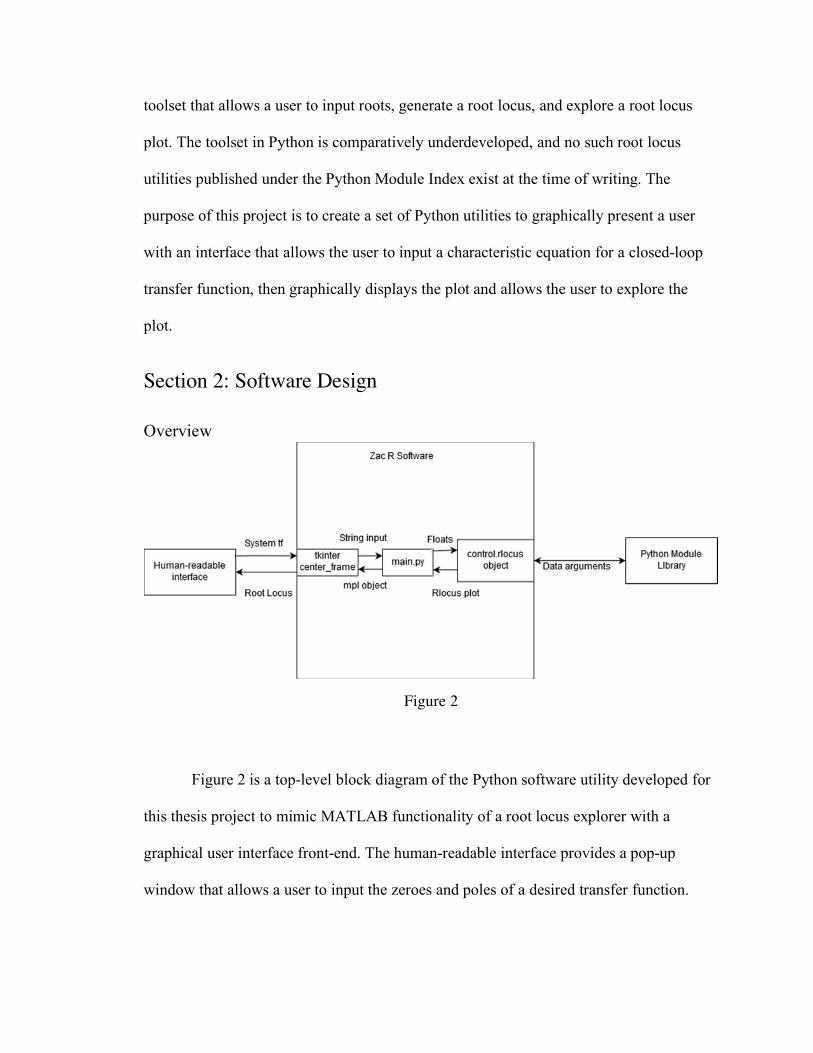
Figure 2

Figure 2 is a top-level block diagram of the Python software utility developed for

this thesis project to mimic MATLAB functionality of a root locus explorer with a

graphical user interface front-end. The human-readable interface provides a pop-up

window that allows a user to input the zeroes and poles of a desired transfer function.

This input is translated to a transfer function and the root locus is generated in a pop-up

figure window.

The root locus backend: control in Python

The control library, at the time of this writing, is not a member of the Python

Module Index [4] and is thus not officially standardized for Python users and must be

installed with Python’s pip package manager.

It provides a comprehensive backend for control systems utilities, such as

transfer function and state space types, but is obfuscated by an object-oriented interface

such that it is not approachable by those uninitiated in software. This library thus does not

meet the same standard of simplicity shown in MATLAB’s standard rlocus() function.

The control library was utilized in the development of this software to provide a backend

for the root locus types and approximate MATLAB functionality.

Presentation to the user: tkinter in Python

The tkinter software library is the set of standard Python calls that implement Tcl,

or Tool Command Language. This library, at the time of writing, is included in the

Python Module Index [4] and thus is standardized across Python implementations and

does not require additional installations.

The tkinter library was utilized in this software as a front-end for the user. A Tk()

object runs the main loop of the graphical window. A ttk.Frame() object is contained by

the Tk() object, and contains a ttk.Button() that maps to a parsing function that sends

arguments to a constructor for the control library’s utilities. Then, the command function

calls a matplotlib object to display a new window containing the root locus.

Section 3: Tests & Results

This section involves documenting the capability of the existing MATLAB

utilities and then displaying a functional analog of these capabilities in the Python

program. Table 1 and Table 2 on the following pages display evidence of the near-

identical functionality of the Python code when compared to the existing MATLAB

utilities. The difference in the figures are largely due to scale and thus superficial.

The tables are formatted to display the transfer function of a closed-loop system,

followed by the depiction of the root locus as provided by the MATLAB built-in root

locus function and then as provided by the software utility developed.

Transfer function examples were provided by MATLAB sample code in [1]

Control Systems Engineering, 7e by Norman S. Nise and by assignment through the

supervisor of this work, Dr. Compeau.

Transfer Function MATLAB rootlocusexplorer.py

! + 52! + 3

! + 45.7!) + 5!* + 20!

Table 1

Transfer Function MATLAB rootlocusexplorer.py

2!* + 5! + 1!* + 2! + 3

! + 3!) + 5!* + 3! + 1

Table 2

Conclusions

The software utility, as of this writing, is functionally complete with respect to the

initial requirements set forth by Dr. Compeau. The Python utility created for this project

was required to fulfill functional equivalence to that of MATLAB’s built-in root locus

plotter.

There are, however, a few behavioral differences that could be addressed in the

program that would make it a stronger utility for root locus exploration. Primarily, the

features that could be added and bugs that could be addressed lie in presentability and

user input.

The software utility does not provide intuitive error responses when a bad input is

given or when an internal failure is logged. The runtime exceptions currently thrown by

the software are either ignored or presented such that they are not approachable to the

target demographic of this utility. Further work could be done to sanitize user input more

thoroughly and to address any errors that arise from either incorrect input or internal

error.

Additionally, the software utility does not have an intuitive way to size the axes of

an outputted figure or edit the range of gains for the root locus. The figure supports zoom

but does not allow vertical and horizontal bounds to be specified by the user. Adding

support for user-specified boundaries of axes and user-specified gains is another area

with the potential for further work.

Appendices

This section contains rudimentary instructions on how to run the software as well

as the source code for the software. A more accessible text file for the code is uploaded

on the author’s github at https://github.com/inducteur/thesis-code

Assume that the github version is the most current and functional version of the

software. This software is meant to be executed from a shell as a script; behavior may be

erratic in iPython or Jupyter.

To install the control library, call pip from the relevant interpreter shell. For

Linux systems, use sudo python3 -m pip3 install control

Please refer to the github README and contact for any further questions.

The following is a paste of the source code for the project at the time of writing. This

paste may differ from the github version.

import tkinter as tkinter import matplotlib as matplotlib from matplotlib import pyplot as plt import numpy as np import control as control from tkinter import ttk from tkinter import * plt.style.use('classic') def plot(): numerator_tf_arg = numerator.get().split(" ") denominator_tf_arg = denominator.get().split(" ") numerator_tf_arg = [float(zeroes) for zeroes in numerator_tf_arg] denominator_tf_arg = [float(poles) for poles in denominator_tf_arg]

rlist, klist = control.root_locus(control.TransferFunction(numerator_tf_arg, denominator_tf_arg), kvect=np.linspace(100.0, -100.0, num=1000)) try: plt.show() except: pass # setup unchanging GUI stuff master_window = tkinter.Tk() master_window.title("Root Locus Explorer") # window name center_frame = tkinter.ttk.Frame(master_window, padding='20 20 20 20') # frame widget #center_frame = tkinter.ttk.Frame(master_window, width=500, height=500, padding='20 20 20 20') # frame widget center_frame.grid(column=0, row=0, sticky=('N, W, E, S')) master_window.columnconfigure(0, weight=1) master_window.rowconfigure(0, weight=1) # bind entry variables numerator = StringVar() denominator = StringVar() sys_numerator_entry = tkinter.ttk.Entry(center_frame, width=10, textvariable=numerator) # width controls the entry box size sys_denominator_entry = tkinter.ttk.Entry(center_frame, width=10, textvariable=denominator)

# define placement of grids for bound vars sys_numerator_entry.grid(column=2, row=4, sticky=(W, E)) sys_denominator_entry.grid(column=2, row=8, sticky=(W, E)) # configure entry button. this button executes whatever function "command" is test_button = tkinter.ttk.Button(center_frame, text='Plot Root Locus', command=plot) test_button.grid(column=14, row=1, sticky=W) ttk.Label(center_frame, text="Input transfer function, separated by spaces\n\n").grid(column=1, row=1, sticky=E) ttk.Label(center_frame, text="numerator").grid(column=3, row=4, sticky=W) ttk.Label(center_frame, text="denominator").grid(column=3, row=8, sticky=W)

master_window.mainloop()

Works Cited

[1] Nise, Norman S. 9. Design Via Root Locus. Control Systems Engineering, 7e. 2015

[2] https://www.mathworks.com/pricing-

licensing.html?prodcode=ML&intendeduse=comm#concurrent

[3] Boyce, William E. and DiPrima, Richard C. Complex Roots of the Characteristic

Equation. Elementary Differential Equations and Boundary Value Problems, 10e. 2012

[4] https://docs.python.org/3/py-modindex.html