Embed Size (px)
Citation preview
Consistency Index (CI)
• minimum number of changes divided by the number required on the tree.
• CI=1 if there is no homoplasy
• negatively correlated with the number of species sampled

Retention Index (RI)
RI =MaxSteps− ObsSteps
MaxSteps−MinSteps
• defined to be 0 for parsimony uninformative characters
• RI=1 if the character fits perfectly
• RI=0 if the tree fits the character as poorly as possible
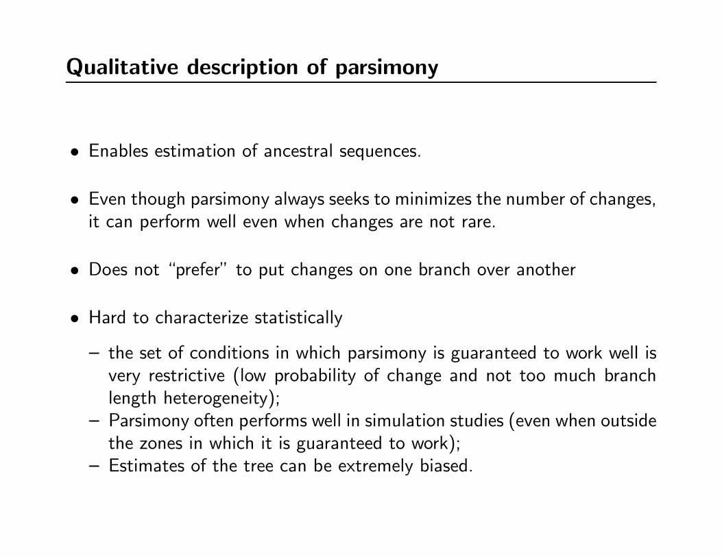
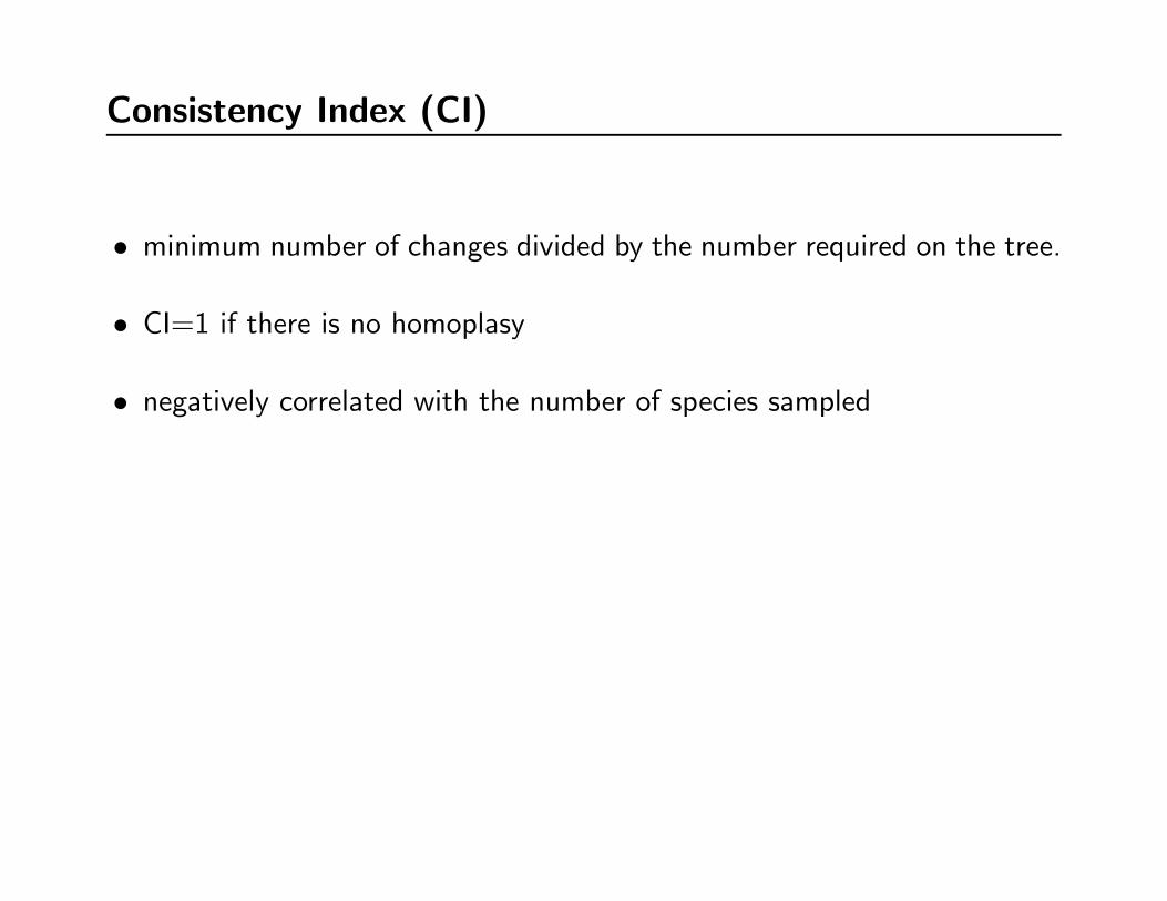
Qualitative description of parsimony
• Enables estimation of ancestral sequences.
• Even though parsimony always seeks to minimizes the number of changes,it can perform well even when changes are not rare.
• Does not “prefer” to put changes on one branch over another
• Hard to characterize statistically
– the set of conditions in which parsimony is guaranteed to work well isvery restrictive (low probability of change and not too much branchlength heterogeneity);
– Parsimony often performs well in simulation studies (even when outsidethe zones in which it is guaranteed to work);
– Estimates of the tree can be extremely biased.

Long branch attraction
Felsenstein, J. 1978. Cases in which
parsimony or compatibility methods will be
positively misleading. Systematic Zoology
27: 401-410.
1.0 1.0
0.010.010.01

Long branch attraction
Felsenstein, J. 1978. Cases in which
parsimony or compatibility methods will be
positively misleading. Systematic Zoology
27: 401-410.
The probability of a parsimony informative
site due to inheritance is very low,
(roughly 0.0003).
A G
A G
1.0 1.0
0.010.010.01
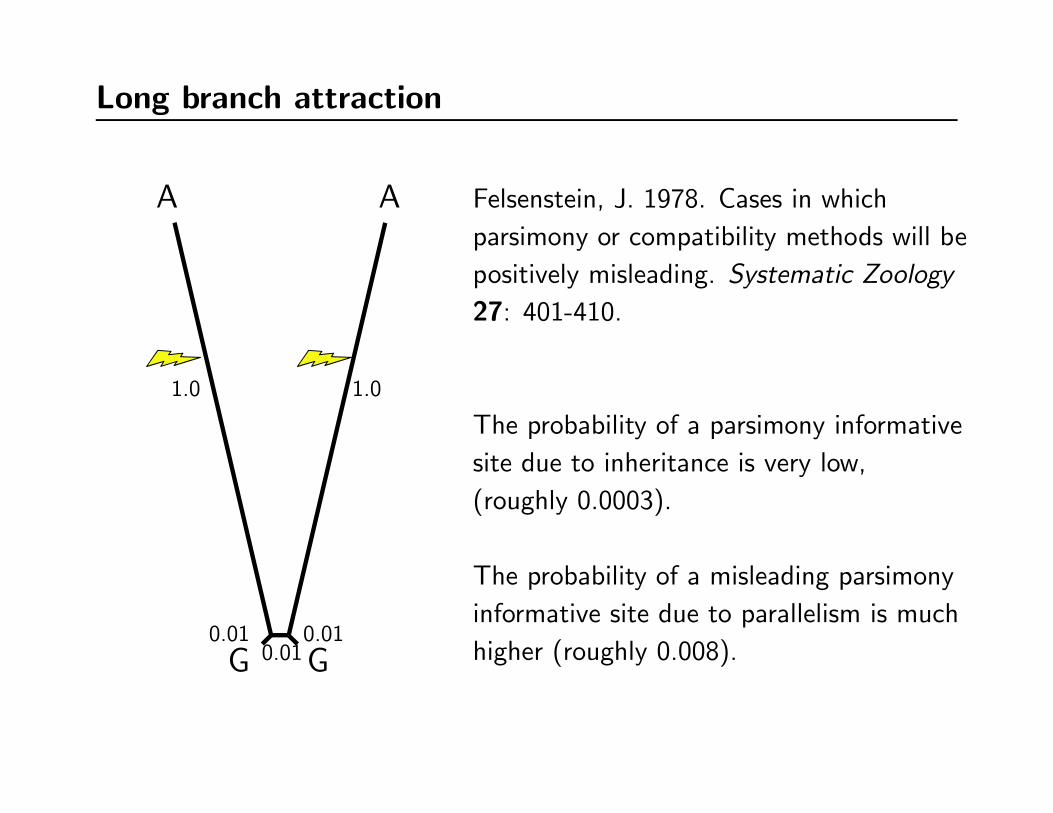
Long branch attraction
Felsenstein, J. 1978. Cases in which
parsimony or compatibility methods will be
positively misleading. Systematic Zoology
27: 401-410.
The probability of a parsimony informative
site due to inheritance is very low,
(roughly 0.0003).
The probability of a misleading parsimony
informative site due to parallelism is much
higher (roughly 0.008).
A A
G G
1.0 1.0
0.010.010.01

Long branch attraction
Parsimony is almost guaranteed to get this tree wrong.1 3
2 4True
1 3
2 4
Inferred

Inconsistency
• Statistical Consistency (roughly speaking) is converging to the trueanswer as the amount of data goes to ∞.
• Parsimony based tree inference is not consistent for some tree shapes. Infact it can be “positively misleading”:
– “Felsenstein zone” tree– Many clocklike trees with short internal branch lengths and long
terminal branches (Penny et al., 1989, Huelsenbeck and Lander,2003).
• Methods for assessing confidence (e.g. bootstrapping) will indicate thatyou should be very confident in the wrong answer.
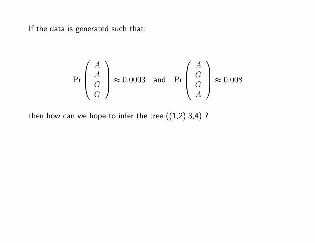
If the data is generated such that:
Pr
AAGG
≈ 0.0003 and Pr
AGGA
≈ 0.008
then how can we hope to infer the tree ((1,2),3,4) ?
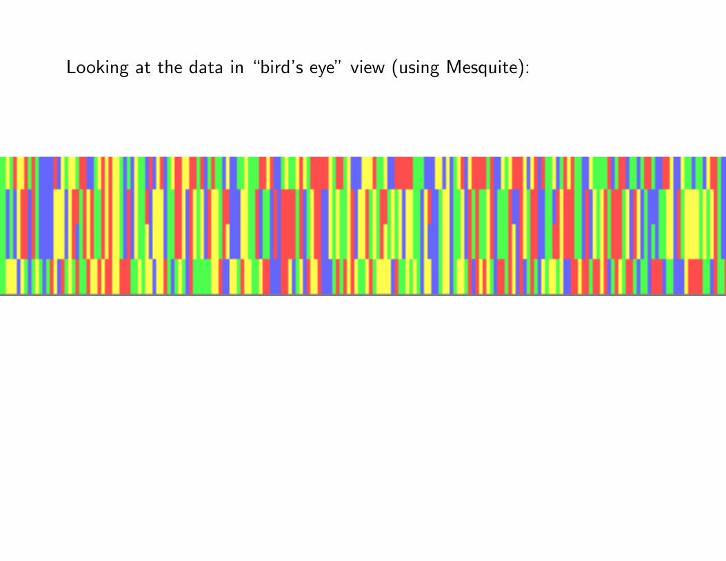
Looking at the data in “bird’s eye” view (using Mesquite):

Looking at the data in “bird’s eye” view (using Mesquite):
We see that sequences 1 and 4 are clearly very different.Perhaps we can estimate the tree if we use the branch length informationfrom the sequences...
Distance-based approaches to inferring trees
• Convert the raw data (sequences) to a pairwise distances
• Try to find a tree that explains these distances.
• Not simply clustering the most similar sequences.

1 2 3 4 5 6 7 8 9 10Species 1 C G A C C A G G T ASpecies 2 C G A C C A G G T ASpecies 3 C G G T C C G G T ASpecies 4 C G G C C A T G T A
Can be converted to a distance matrix:
Species 1 Species 2 Species 3 Species 4Species 1 0 0 0.3 0.2Species 2 0 0 0.3 0.2Species 3 0.3 0.3 0 0.3Species 4 0.2 0.2 0.3 0

Note that the distance matrix is symmetric.
Species 1 Species 2 Species 3 Species 4Species 1 0 0 0.3 0.2Species 2 0 0 0.3 0.2Species 3 0.3 0.3 0 0.3Species 4 0.2 0.2 0.3 0

. . . so we can just use the lower triangle.
Species 1 Species 2 Species 3Species 2 0Species 3 0.3 0.3Species 4 0.2 0.2 0.3
Can we find a tree that would predict these observed character divergences?
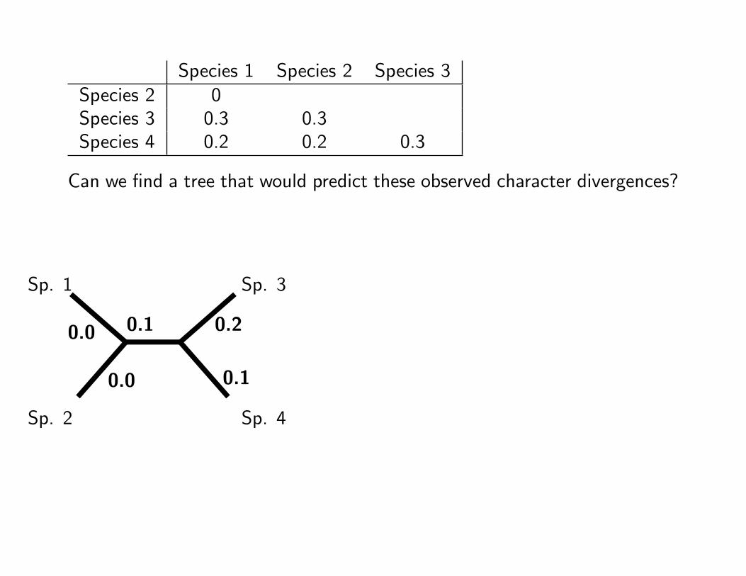
Species 1 Species 2 Species 3Species 2 0Species 3 0.3 0.3Species 4 0.2 0.2 0.3
Can we find a tree that would predict these observed character divergences?
Sp. 1
Sp. 2
Sp. 3
Sp. 4
0.0
0.0
0.1 0.2
0.1

1
2
3
4
a
b
c
d
i
1 2 32 d12
3 d13 d23
4 d14 d24 d34
dataparameters
p12 = a+ b
p13 = a+ i+ c
p14 = a+ i+ d
p23 = b+ i+ c
p23 = b+ i+ d
p34 = c+ d

If our pairwise distance measurements were error-free estimates
of the evolutionary distance between the sequences, then we
could always infer the tree from the distances.
The evolutionary distance is the number of mutations that have
occurred along the path that connects two tips.
We hope the distances that we measure can produce good
estimates of the evolutionary distance, but we know that they
cannot be perfect.
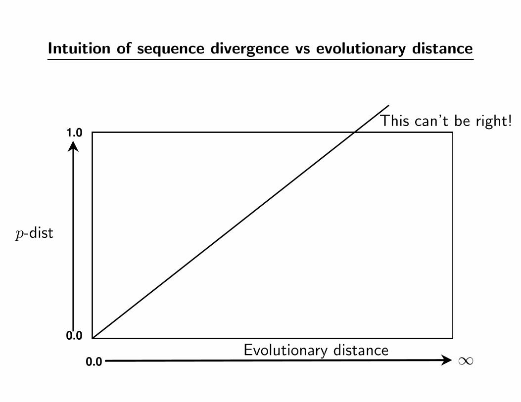
Intuition of sequence divergence vs evolutionary distance
0.0
1.0
0.0
p-dist
Evolutionary distance ∞
This can’t be right!
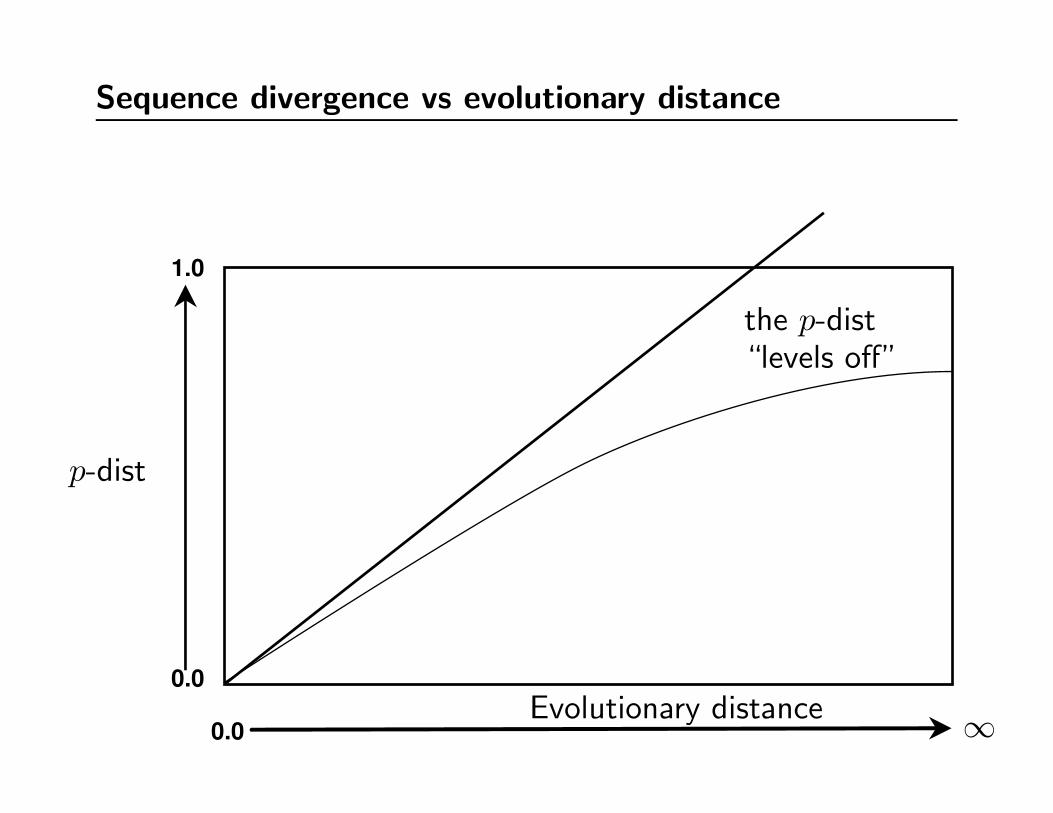
Sequence divergence vs evolutionary distance
0.0
1.0
0.0
p-dist
Evolutionary distance ∞
the p-dist“levels off”

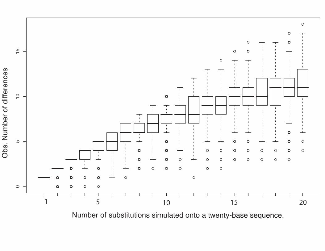
“Multiple hits” problem (also known as saturation)
• Levelling off of sequence divergence vs time plot is caused by
multiple substitutions affecting the same site in the DNA.
• At large distances the “raw” sequence divergence (also known
as the p-distance or Hamming distance) is a poor estimate
of the true evolutionary distance.
• Large p-distances respond more to model-based correction –
and there is a larger error associated with the correction.
05
1015
Obs
. Num
ber o
f diff
eren
ces
Number of substitutions simulated onto a twenty-base sequence.
1 5 10 15 20

Distance corrections
• applied to distances before tree estimation,
• converts raw distances to an estimate of the evolutionary
distance
d = −34
ln(
4c3− 1)
1 2 3
2 d12
3 d13 d23
4 d14 d24 d34
corrected distances
1 2 3
2 c123 c13 c234 c14 c24 c34
“raw” p-distances

d = −34
ln(
1− 4c3
)
1 2 3
2 03 0.383 0.3834 0.233 0.233 0.383
corrected distances
1 2 3
2 0.03 0.3 0.34 0.2 0.2 0.3
“raw” p-distances
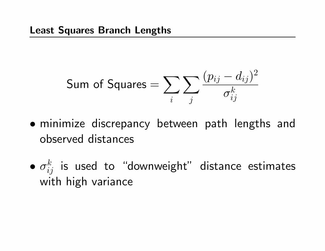
Least Squares Branch Lengths
Sum of Squares =∑i
∑j
(pij − dij)2
σkij
• minimize discrepancy between path lengths and
observed distances
• σkij is used to “downweight” distance estimates
with high variance
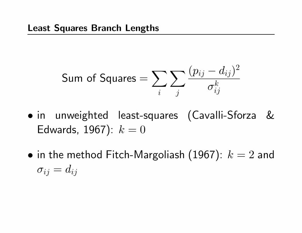
Least Squares Branch Lengths
Sum of Squares =∑i
∑j
(pij − dij)2
σkij
• in unweighted least-squares (Cavalli-Sforza &
Edwards, 1967): k = 0
• in the method Fitch-Margoliash (1967): k = 2 and
σij = dij

Poor fit using arbitrary branch lengths
Species dij pij (p− d)2Hu-Ch 0.09267 0.2 0.01152
Hu-Go 0.10928 0.3 0.03637
Hu-Or 0.17848 0.4 0.04907
Hu-Gi 0.20420 0.4 0.03834
Ch-Go 0.11440 0.3 0.03445
Ch-Or 0.19413 0.4 0.04238
Ch-Gi 0.21591 0.4 0.03389
Go-Or 0.18836 0.3 0.01246
Go-Gi 0.21592 0.3 0.00707
Or-Gi 0.21466 0.2 0.00021
S.S. 0.26577
Hu
Ch
Go
Or
Gi
0.1
0.1
0.1 0.1
0.1
0.1
0.1

Optimizing branch lengths yields the least-squares score
Species dij pij (p− d)2Hu-Ch 0.09267 0.09267 0.000000000Hu-Go 0.10928 0.10643 0.000008123Hu-Or 0.17848 0.18026 0.000003168Hu-Gi 0.20420 0.20528 0.000001166Ch-Go 0.11440 0.11726 0.000008180Ch-Or 0.19413 0.19109 0.000009242Ch-Gi 0.21591 0.21611 0.000000040Go-Or 0.18836 0.18963 0.000001613Go-Gi 0.21592 0.21465 0.000001613Or-Gi 0.21466 0.21466 0.000000000
S.S. 0.000033144
Hu
Ch
Go
Or
Gi
0.04092
0.05175
0.00761 0.03691
0.05790
0.09482
0.11984
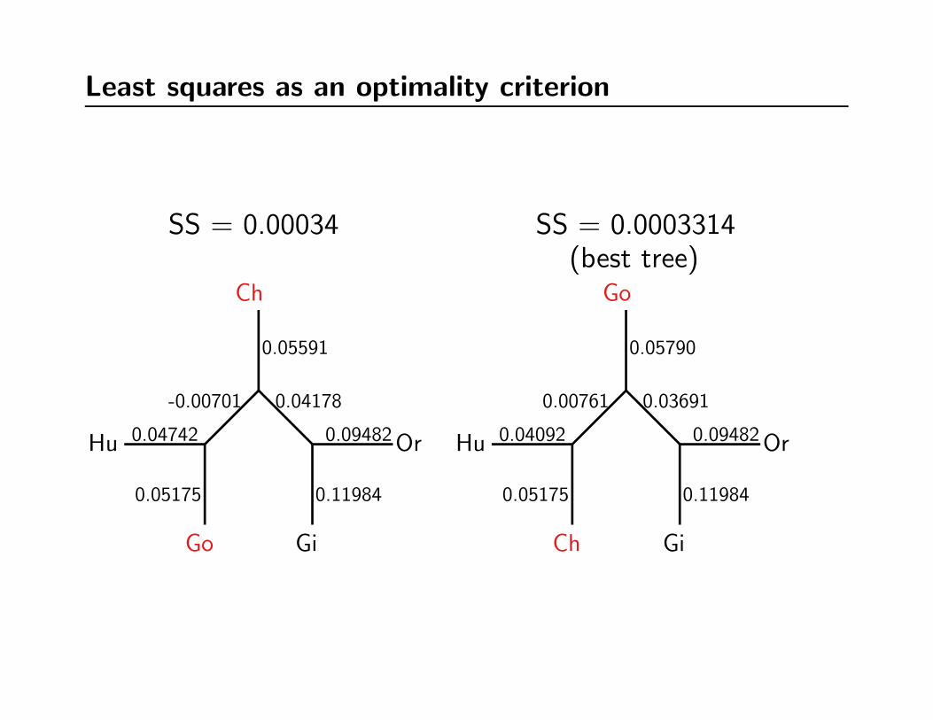
Least squares as an optimality criterion
Hu
Ch
Go
Or
Gi
0.04092
0.05175
0.00761 0.03691
0.05790
0.09482
0.11984
Hu
Go
Ch
Or
Gi
0.04742
0.05175
-0.00701 0.04178
0.05591
0.09482
0.11984
SS = 0.00034 SS = 0.0003314(best tree)
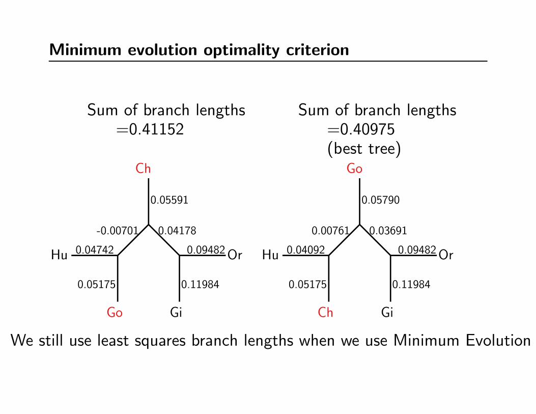
Minimum evolution optimality criterion
Hu
Ch
Go
Or
Gi
0.04092
0.05175
0.00761 0.03691
0.05790
0.09482
0.11984
Hu
Go
Ch
Or
Gi
0.04742
0.05175
-0.00701 0.04178
0.05591
0.09482
0.11984
Sum of branch lengths=0.41152
Sum of branch lengths=0.40975(best tree)
We still use least squares branch lengths when we use Minimum Evolution
Huson and Steel – distances that perfectly mislead
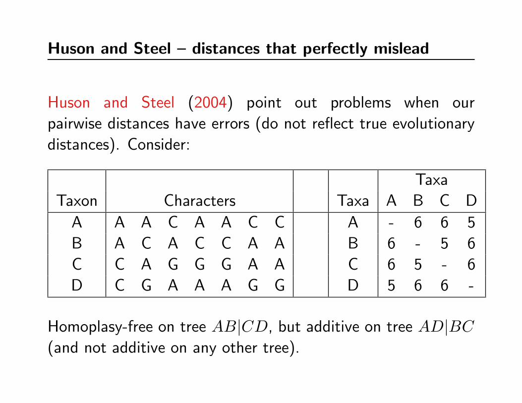
Huson and Steel (2004) point out problems when our
pairwise distances have errors (do not reflect true evolutionary
distances). Consider:
Taxa
Taxon Characters Taxa A B C D
A A A C A A C C A - 6 6 5
B A C A C C A A B 6 - 5 6
C C A G G G A A C 6 5 - 6
D C G A A A G G D 5 6 6 -
Homoplasy-free on tree AB|CD, but additive on tree AD|BC(and not additive on any other tree).
Huson and Steel – distances that perfectly mislead
Clearly, the previous matrix was contrived and not typical of
realistic data.
Would we ever expect to see additive distances on the wrongtree as the result of a reasonable evolutionary process?
Yes.
Huson and Steel (2004) show that under the equal-input
model(more on this later), the uncorrected distances can be
additive on the wrong tree leading to long-branch attraction.
The result holds even if the number of characters →∞

Failure to correct distance sufficiently leads to poorperformance
“Under-correcting” will underestimate long evolutionary
distances more than short distances
1 2
3 4
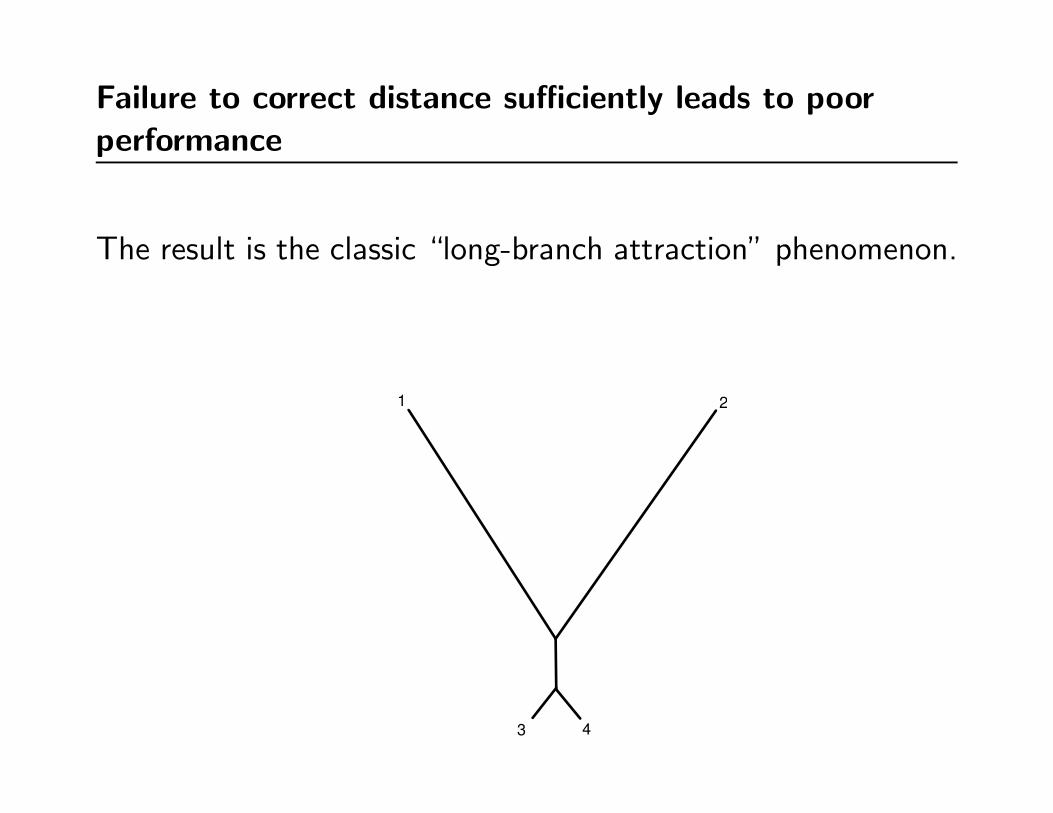
Failure to correct distance sufficiently leads to poorperformance
The result is the classic “long-branch attraction” phenomenon.
1 2
3 4

Distance methods – summary
We can:
• summarize a dataset as a matrix of distances or dissimilarities.
• correct these distances for unseen character state changes.
• estimate a tree by finding the tree with path lengths that are
“closest” to the corrected distances.

A
B
C
D
a
b
c
d
i
@@@@@@@@
��������
��������
@@@@@@@@
A B C
B dABC dAC dBCD dAD dBD dCD

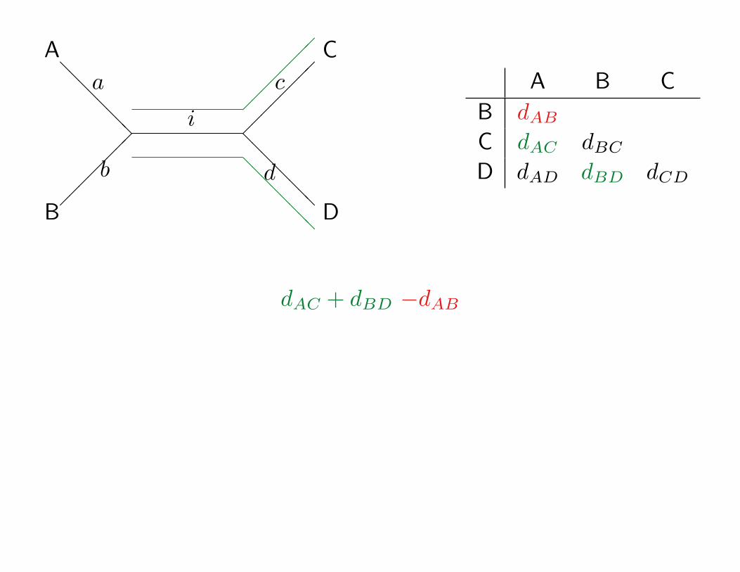
If the tree above is correct then:
pAB = a+ b
pAC = a+ i+ c
pAD = a+ i+ d
pBC = b+ i+ c
pBD = b+ i+ d
pCD = c+ d

A
B
C
D
a
b
c
d
i
@@@@@@@@
��������
��������
@@@@@@@@
@@@@@@@@ �
�������
A B C
B dABC dAC dBCD dAD dBD dCD
dAC

A
B
C
D
a
b
c
d
i
@@@@@@@@
��������
��������
@@@@@@@@
@@@@@@@@ �
�������
�������� @
@@@@@@@
A B C
B dABC dAC dBCD dAD dBD dCD
dAC + dBD

A
B
C
D
a
b
c
d
i
@@@@@@@@
��������
��������
@@@@@@@@
@@@@@@@@ �
�������
�������� @
@@@@@@@
��������
@@@@@@@@
A B C
B dABC dAC dBCD dAD dBD dCD
dAC + dBD
dAB
A
B
C
D
a
b
c
d
i
@@@@@@@@
��������
��������
@@@@@@@@
��������
@@@@@@@@
A B C
B dABC dAC dBCD dAD dBD dCD
dAC + dBD −dAB
A
B
C
D
a
b
c
d
i
@@@@@@@@
��������
��������
@@@@@@@@
��������
@@@@@@@@
��������
@@@@@@@@
A B C
B dABC dAC dBCD dAD dBD dCD
dAC + dBD −dAB
dCD
A
B
C
D
a
b
c
d
i
@@@@@@@@
��������
��������
@@@@@@@@
A B C
B dABC dAC dBCD dAD dBD dCD
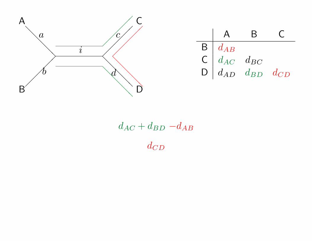
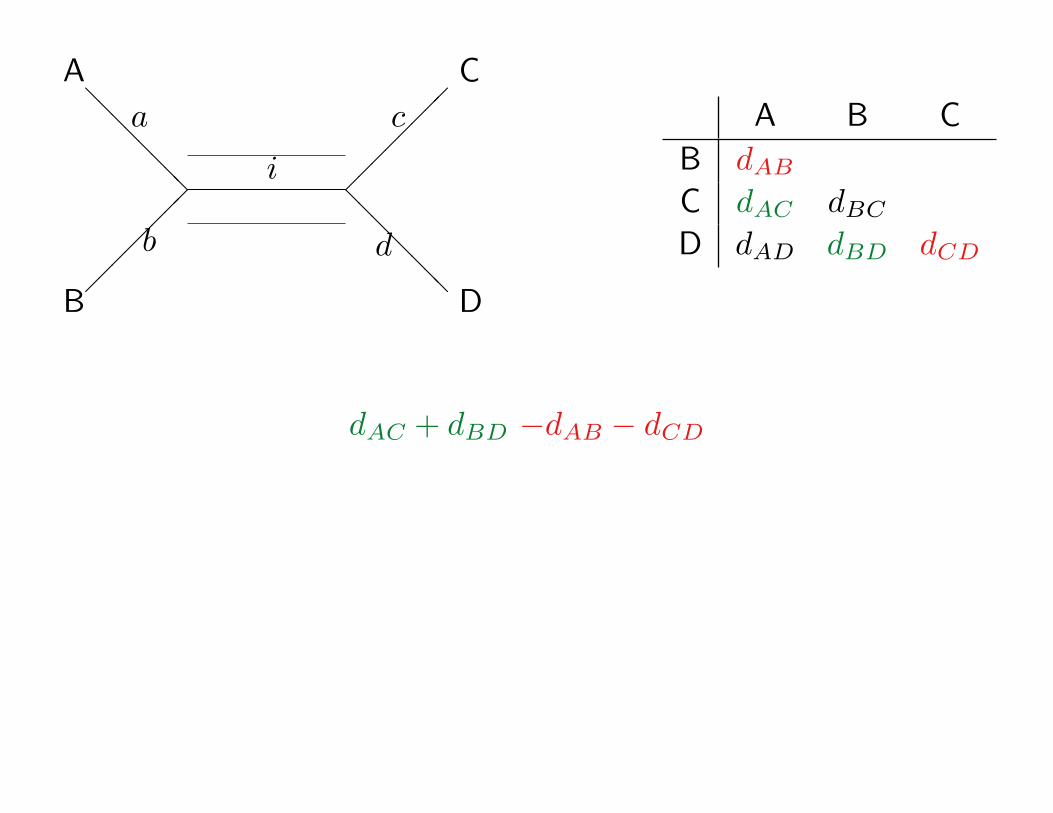
dAC + dBD −dAB − dCD

A
B
C
D
a
b
c
d
i
@@@@@@@@
��������
��������
@@@@@@@@
A B C
B dABC dAC dBCD dAD dBD dCD
i† = dAC+dBD−dAB−dCD2
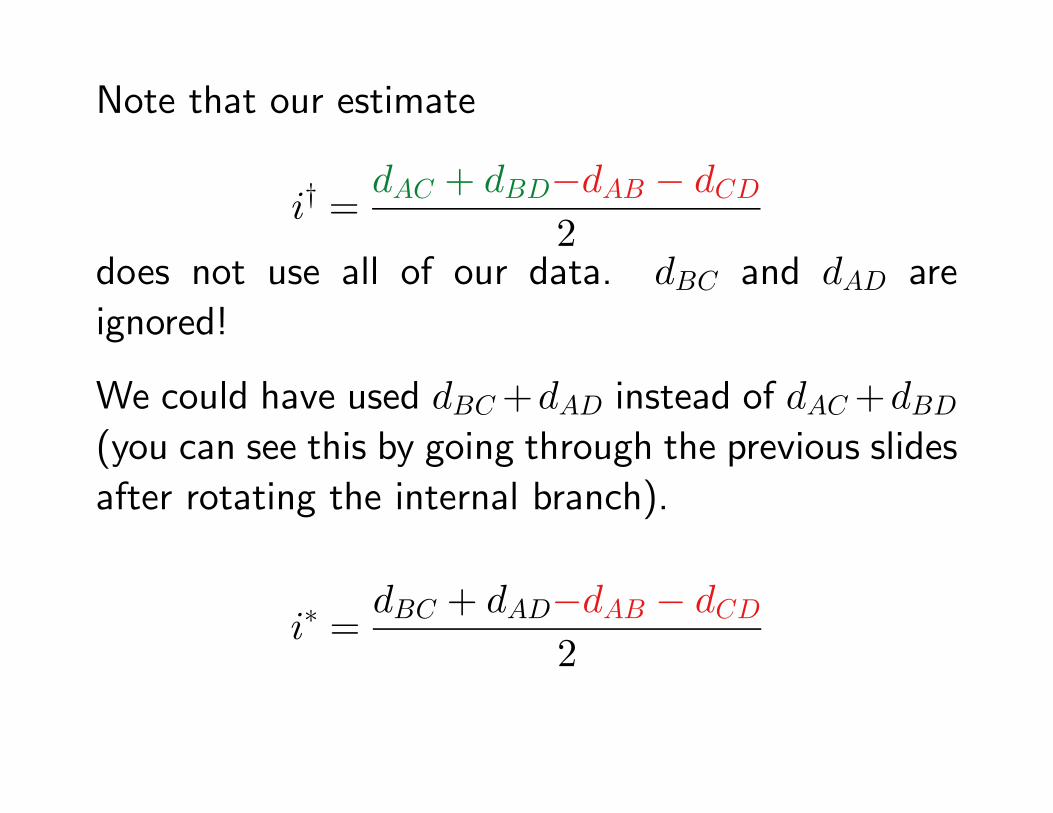
Note that our estimate
i† =dAC + dBD−dAB − dCD
2does not use all of our data. dBC and dAD are
ignored!
We could have used dBC +dAD instead of dAC +dBD(you can see this by going through the previous slides
after rotating the internal branch).
i∗ =dBC + dAD−dAB − dCD
2
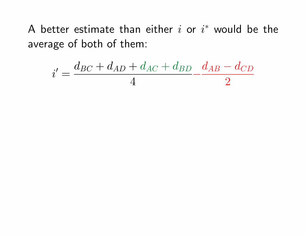
A better estimate than either i or i∗ would be the
average of both of them:
i′ =dBC + dAD + dAC + dBD
4−dAB − dCD
2

A
B
C
D
νa
νb
νc
νd
νi
@@@@@@
������
������
@@@@@@
A
C
B
D
νa
νc
νb
νd
νi
@@@@@@
������
������
@@@@@@
A
D
C
B
νa
νd
νc
νb
νi
@@@@@@
������
������
@@@@@@
dAB + dCD νa + νb + νc + νd νa+νb+νc+νd+2νi νa + νb + νc + νd + 2νi
dAC + dBD νa+νb+νc+νd+2νi νa + νb + νc + νd νa + νb + νc + νd + 2νi
dAD + dBC νa+νb+νc+νd+2νi νa+νb+νc+νd+2νi νa + νb + νc + νd
The four point condition of Buneman (1971).
This assumes additivity of distances.

A
C
B
D
νa
νc
νb
νd
νi
@@@@@@
������
������
@@@@@@
dAB + dCD νa + νb + νc + νd + 2νi + εAB + εCD
dAC + dBD νa + νb + νc + νd + εAC + εBD
dAD + dBC νa + νb + νc + νd + 2νi + εAD + εBC
If |εij| < νi2 then dAC + dBD will still be the smallest sum – So
Buneman’s method will get the tree correct.
Worst case: εAC = εBD = νi2 and εAB = εCD = −νi2 then
dAC + dBD = νa + νb + νc + νd + νi = dAB + dCD
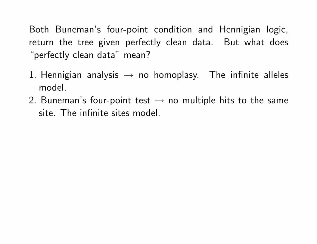
Both Buneman’s four-point condition and Hennigian logic,
return the tree given perfectly clean data. But what does
“perfectly clean data” mean?
1. Hennigian analysis → no homoplasy. The infinite alleles
model.
2. Buneman’s four-point test → no multiple hits to the same
site. The infinite sites model.

The guiding principle of distance-based methods
If our data are true measures of evolutionary distances (and the
distance along each branch is always > 0) then:
1. The distances will be additive on the true tree.
2. The distances will not be additive on any other tree.
This is the basis of Buneman’s method and the motivation for
minimizing the sum-of-squared error (least squares) too choose
among trees.

Balanced minimum evolution
The logic behind Buneman’s four-point condition has been
extend to trees of more than 4 taxa by Pauplin (2000) and
Semple and Steel (2004).
Pauplin (2000) showed that you can calculate a tree length
from the pairwise distances without calculating branch lengths.
The key is weighting the distances:
l =N∑i
N∑j=i+1
wijdij
where:
wij =1
2n(i,j)
and n(i, j) is the number of nodes on the path from i to j.

Balanced minimum evolution
“Balanced Minimum Evolution” Desper and Gascuel (2002,
2004) – fitting the branch lengths using the estimators of
Pauplin (2000) and preferring the tree with the smallest tree
length
BME = a form of weighted least squares in which distances are
down-weighted by an exponential function of the topological
distances between the leaves.
Desper and Gascuel (2005): neighbor-joining is star
decomposition (more on this later) under BME. See Gascuel
and Steel (2006)
FastME
Software by Desper and Gascuel (2004) which implements
searching under the balanced minimum evolution criterion.
It is extremely fast and is more accurate than neighbor-joining
(based on simulation studies).

Distance methods: pros
• Fast – the new FastTree method Price et al. (2009) can
calculate a tree in less time than it takes to calculate a full
distance matrix!
• Can use models to correct for unobserved differences
• Works well for closely related sequences
• Works well for clock-like sequences
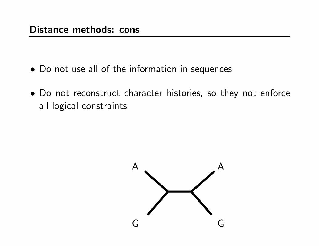
Distance methods: cons
• Do not use all of the information in sequences
• Do not reconstruct character histories, so they not enforce
all logical constraints
A
G
A
G

Neighbor-joining
Saitou and Nei (1987). r is the number of leaves remaining.
Start with r = N .
1. choose the pair of leaves x and y that minimize Q(x, y):
Q(i, j) = (r − 2)dij −r∑
k=1
dik −r∑
k=1
djk
2. Join x and y with at a new node z. Take x and y out of
the leaf set and distance matrix, and add the new node z as
a leaf.
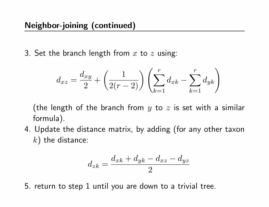
Neighbor-joining (continued)
3. Set the branch length from x to z using:
dxz =dxy2
+(
12(r − 2)
)( r∑k=1
dxk −r∑
k=1
dyk
)
(the length of the branch from y to z is set with a similar
formula).
4. Update the distance matrix, by adding (for any other taxon
k) the distance:
dzk =dxk + dyk − dxz − dyz
2
5. return to step 1 until you are down to a trivial tree.

Neighbor-joining (example)
A B C D E F
A -
B 0.258 -
C 0.274 0.204 -
D 0.302 0.248 0.278 -
E 0.288 0.224 0.252 0.268 -
F 0.250 0.160 0.226 0.210 0.194 -

Neighbor-joining (example)
∑k dik A B C D E F
1.372 A 0.0 0.258 0.274 0.302 0.288 0.25
1.094 B 0.258 0.0 0.204 0.248 0.224 0.16
1.234 C 0.274 0.204 0.0 0.278 0.252 0.226
1.306 D 0.302 0.248 0.278 0.0 0.268 0.21
1.226 E 0.288 0.224 0.252 0.268 0.0 0.194
1.040 F 0.25 0.16 0.226 0.21 0.194 0.0
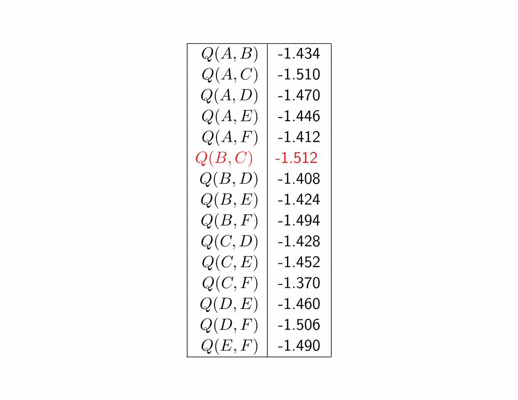
Q(A,B) -1.434
Q(A,C) -1.510
Q(A,D) -1.470
Q(A,E) -1.446
Q(A,F ) -1.412
Q(B,C) -1.512
Q(B,D) -1.408
Q(B,E) -1.424
Q(B,F ) -1.494
Q(C,D) -1.428
Q(C,E) -1.452
Q(C,F ) -1.370
Q(D,E) -1.460
Q(D,F ) -1.506
Q(E,F ) -1.490

Neighbor-joining (example)
A D E F (B,C)
A 0.0 0.302 0.288 0.25 0.164
D 0.302 0.0 0.268 0.21 0.161
E 0.288 0.268 0.0 0.194 0.136
F 0.25 0.21 0.194 0.0 0.091
(B,C) 0.164 0.161 0.136 0.091 0.0
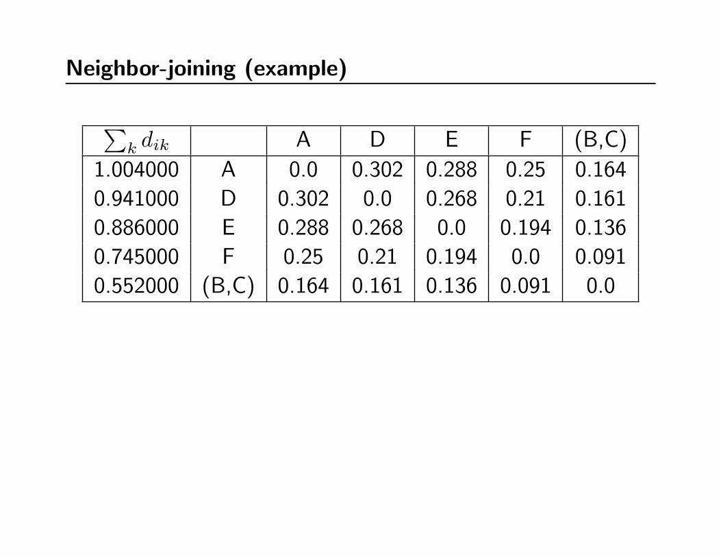
Neighbor-joining (example)
∑k dik A D E F (B,C)
1.004000 A 0.0 0.302 0.288 0.25 0.164
0.941000 D 0.302 0.0 0.268 0.21 0.161
0.886000 E 0.288 0.268 0.0 0.194 0.136
0.745000 F 0.25 0.21 0.194 0.0 0.091
0.552000 (B,C) 0.164 0.161 0.136 0.091 0.0

Neighbor-joining (example)
Q(A,D) -1.039000
Q(A,E) -1.026000
Q(A,F ) -0.999000
Q(A, (B,C)) -1.064000
Q(D,E) -1.023000
Q(D,F ) -1.056000
Q(D, (B,C)) -1.010000
Q(E,F ) -1.049000
Q(E, (B,C)) -1.030000
Q(F, (B,C)) -1.024000
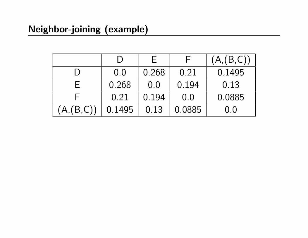
Neighbor-joining (example)
D E F (A,(B,C))
D 0.0 0.268 0.21 0.1495
E 0.268 0.0 0.194 0.13
F 0.21 0.194 0.0 0.0885
(A,(B,C)) 0.1495 0.13 0.0885 0.0

Neighbor-joining (example)
∑k dik D E F (A,(B,C))
0.627500 D 0.0 0.268 0.21 0.1495
0.592000 E 0.268 0.0 0.194 0.13
0.492500 F 0.21 0.194 0.0 0.0885
0.368000 (A,(B,C)) 0.1495 0.13 0.0885 0.0

Neighbor-joining (example)
Q(D,E) -0.683500
Q(D,F ) -0.700000
Q(D, (A, (B,C))) -0.696500
Q(E,F ) -0.696500
Q(E, (A, (B,C))) -0.700000
Q(F, (A, (B,C))) -0.683500
((D,F ), E, (A, (B,C)))

Neighbor-joining is special
Bryant (2005) discusses neighbor joining in the context of
clustering methods that:
• Work on the distance (or dissimilarity) matrix as input.
• Repeatedly
– select a pair of taxa to agglomerate (step 1 above)
– make the pair into a new group (step 2 above)
– estimate branch lengths (step 3 above)
– reduce the distance matrix (step 4 above)

Neighbor-joining is special (cont)
Bryant (2005) shows that if you want your selection criterion
to be:
• based solely on distances
• invariant to the ordering of the leaves (no a priori special
taxa).
• work on linear combinations of distances (simple coefficients
for weights, no fancy weighting schemes).
• statistically consistent
then neighbor-joining’s Q-criterion as a selection rule is the
only choice.
Neighbor-joining is not perfect
• BioNJ (Gascuel, 1997) does a better job by using the variance
and covariances in the reduction step.
• Weighbor (Bruno et al., 2000) includes the variance
information in the selection step.
• FastME (Desper and Gascuel, 2002, 2004) does a better job
of finding the BME tree (and seems to get the true tree right
more often).
References
Bruno, W., Socci, N., and Halpern, A. (2000). Weighted
neighbor joining: A likelihood-based approach to distance-
based phylogeny reconstruction. Molecular Biology and
Evolution, 17(1):189–197.
Bryant, D. (2005). On the uniqueness of the selection criterion
in neighbor-joining. Journal of Classification, 22:3–15.
Buneman, P. (1971). The recovery of trees from measures of
dissimilarity. In Hodson, F. R., Kendall, D. G., and Tautu,
P., editors, Mathematics in the Archaeological and Historical
Sciences, Edinburgh. The Royal Society of London and the
Academy of the Socialist Republic of Romania, Edinburgh
University Press.

Desper, R. and Gascuel, O. (2002). Fast and accurate
phylogeny reconstruction algorithms based on the minimum-
evolution principle. Journal of Computational Biology,
9(5):687–705.
Desper, R. and Gascuel, O. (2004). Theoretical foundation
of the balanced minimum evolution method of phylogenetic
inference and its relationship to weighted least-squares tree
fitting. Molecular Biology and Evolution.
Desper, R. and Gascuel, O. (2005). The minimum evolution
distance-based approach to phylogenetic inference. In
Gascuel, O., editor, Mathematics of Evolution and Phylogeny,
pages 1–32. Oxford University Press.
Gascuel, O. (1997). BIONJ: an improved version of the
NJ algorithm based on a simple model of sequence data.
Molecular Biology and Evolution, 14(7):685–695.
Gascuel, O. and Steel, M. (2006). Neighbor-joining revealed.
Molecular Biology and Evolution, 23(11):1997–2000.
Huson, D. and Steel, M. (2004). Distances that perfectly
mislead. Systematic Biology, 53(2):327–332.
Pauplin, Y. (2000). Direct calculation of a tree length
using a distance matrix. Journal of Molecular Evolution,
2000(51):41–47.
Price, M. N., Dehal, P., and Arkin, A. P. (2009). FastTree:
Computing large minimum-evolution trees with profiles
instead of a distance matrix. Molecular Biology and Evolution,
26(7):1641–1650.

Saitou, N. and Nei, M. (1987). The neighbor-joining method: a
new method for reconstructing phylogenetic trees. Molecular
Biology and Evolution, 4(4):406–425.
Semple, C. and Steel, M. (2004). Cyclic permutations
and evolutionary trees. Advances in Applied Mathematics,
32(4):669–680.