Consideration of Electromagnetic Effects in Aircraft Design

Thomas JerseDepartment of Electrical and Computer Engineering

Sigma Xi Brownbag Presentation10/17/08

Electromagnetic Environmental Effects

• Safety of flight

• Radiation Hazards

• Cosite interference

E3

Who Makes the Rules?

• FAA– DO-160

• JAA

• Department of Defense– MIL-STD-461E– MIL-STD-464A

Safety of Flight

• Power Systems– Fly-by-wire controls

• 3x or 4x redundancy

• Air Traffic Control (ATC) radios

• Navigation Systems

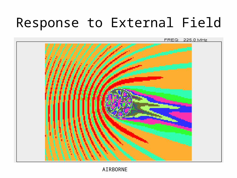
Response to External Field

AIRBORNE

HIRF Testing

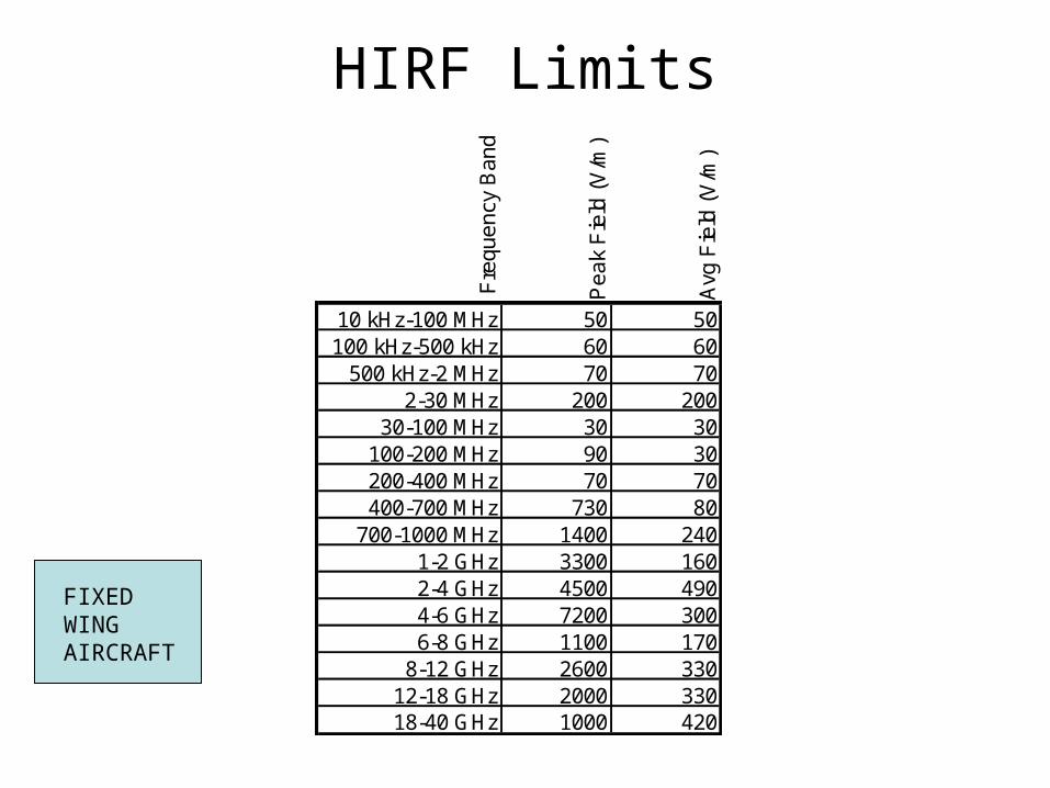
HIRF Limits

Fre

quen

cy B

and

Pea

k F

ield

(V

/m)

Avg

Fie

ld (

V/m

)

10 kHz-100 MHz 50 50100 kHz-500 kHz 60 60

500 kHz-2 MHz 70 702-30 MHz 200 200

30-100 MHz 30 30100-200 MHz 90 30200-400 MHz 70 70400-700 MHz 730 80

700-1000 MHz 1400 2401-2 GHz 3300 1602-4 GHz 4500 4904-6 GHz 7200 3006-8 GHz 1100 170

8-12 GHz 2600 33012-18 GHz 2000 33018-40 GHz 1000 420

FIXEDWINGAIRCRAFT

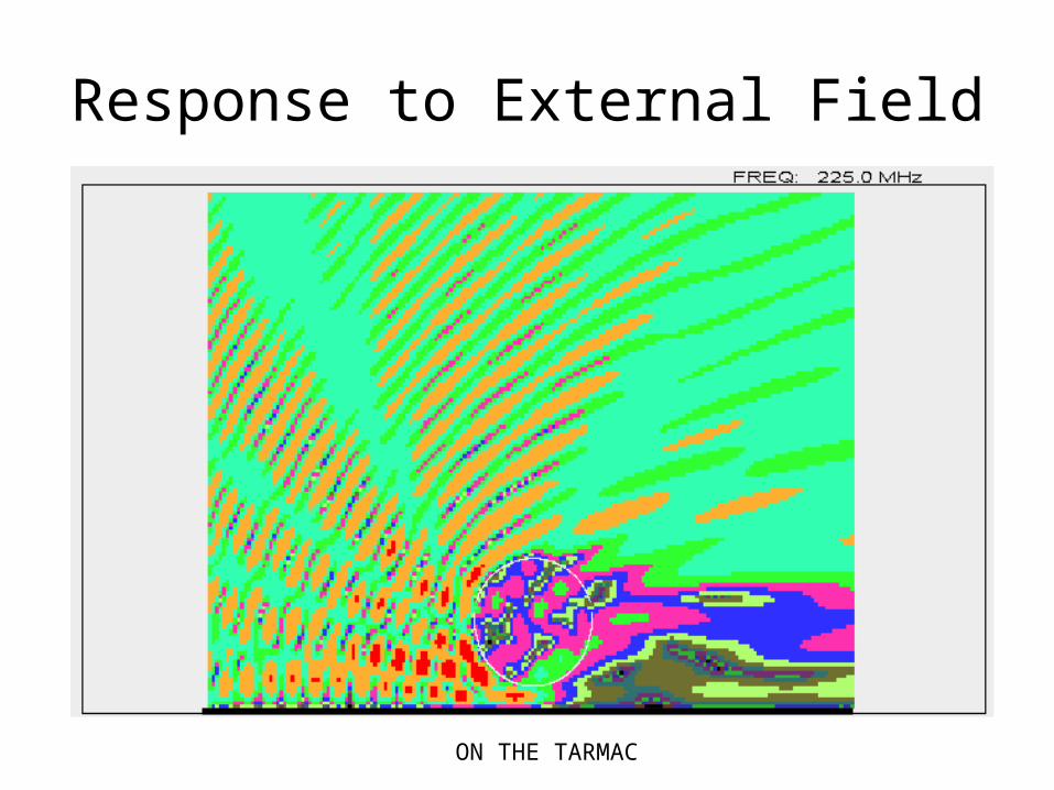
Response to External Field

ON THE TARMAC

Radiation Hazards

• Personnel (RADHAZ)

• Fuel (HERF)

• Ordinance (HERO)

Hazard to Personnel

• 10 W/m2 maximum averaged over a 6 minute period

• Corresponds to 61.4 Vrms/m

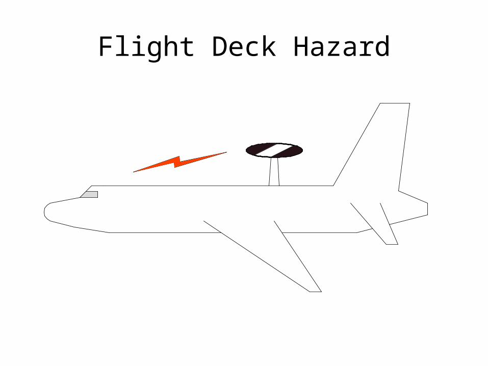
Flight Deck Hazard

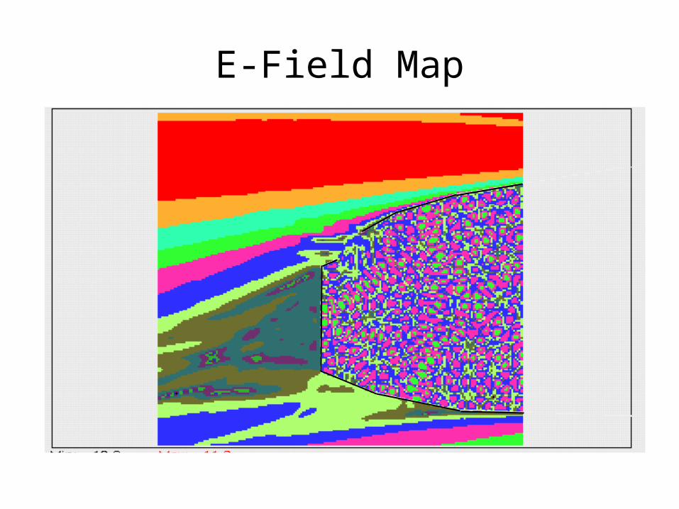
E-Field Map

USS Forrestal

USS Forrestal

USS Forrestal

162 SAILORS PERISHED

Electromagnetic Environmental Effects

• Safety of flight

• Radiation Hazards

• Cosite interference

E3

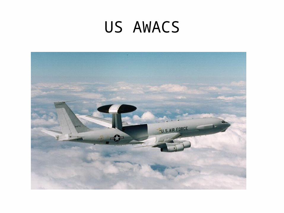
US AWACS

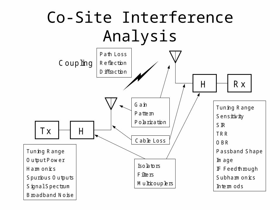
Co-Site Interference Analysis

Tx

Rx

H

H

Output PowerHarmonicsSpurious OutputsSignal Spectrum

Sensitivity

Image

Subharmonics

OBRTRR

Intermods

CouplingPath LossReflectionDiffraction

GainPattern

FiltersMulticouplers

Isolators

Broadband Noise

Tuning Range

Tuning Range

IF Feedthrough

Passband Shape

Cable Loss

Polarization SIR

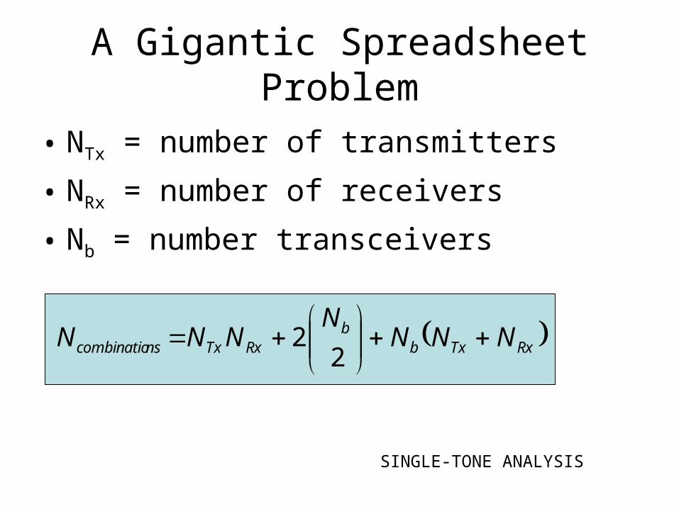
A Gigantic Spreadsheet Problem

• NTx = number of transmitters

• NRx = number of receivers

• Nb = number transceivers

RxTxb

bRxTxnscombinatio NNN

NNNN

22

SINGLE-TONE ANALYSIS

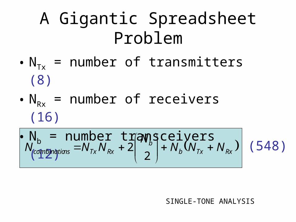
A Gigantic Spreadsheet Problem

• NTx = number of transmitters (8)

• NRx = number of receivers (16)

• Nb = number transceivers (12)

RxTxb

bRxTxnscombinatio NNN

NNNN

22 (548)

SINGLE-TONE ANALYSIS

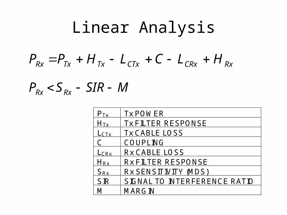
Linear Analysis

MSIRSP RxRx

RxCRxCTxTxTxRx HLCLHPP

PTx Tx POWER HTx Tx FILTER RESPONSE LCTx Tx CABLE LOSS C COUPLING LCRx Rx CABLE LOSS HRx Rx FILTER RESPONSE SRx Rx SENSITIVITY (MDS) SIR SIGNAL TO INTERFERENCE RATIO M MARGIN

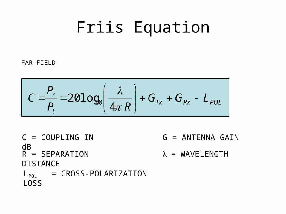
Friis Equation

FAR-FIELD

C = COUPLING IN dB

R = SEPARATION DISTANCE = WAVELENGTH

G = ANTENNA GAIN

POLRxTxt

r LGGRP

PC

4log20 10

L = CROSS-POLARIZATION LOSSPOL

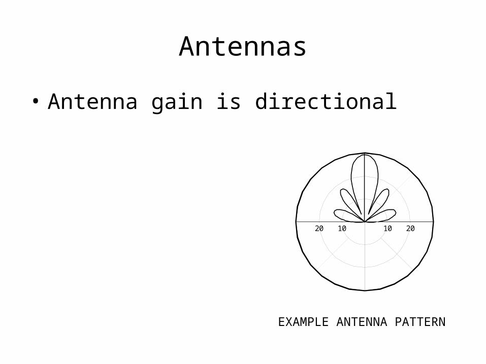
Antennas

• Antenna gain is directional

1010 2020

EXAMPLE ANTENNA PATTERN

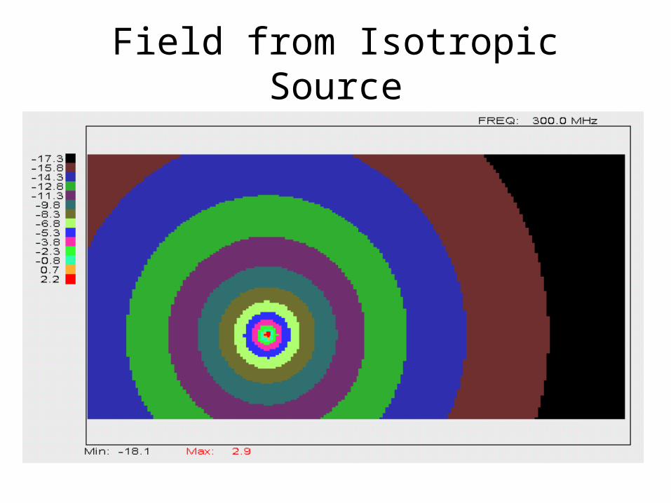
Field from Isotropic Source

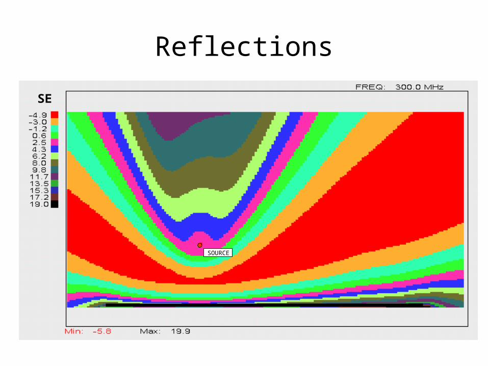
Reflections

SOURCE

SE

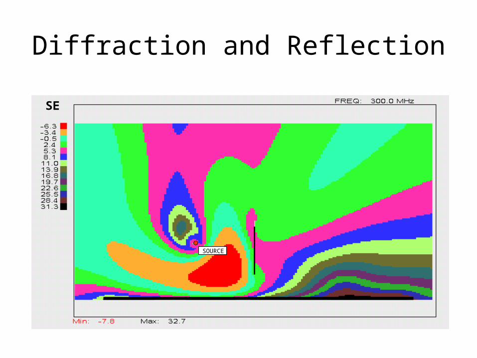
Diffraction and Reflection

SOURCE

SE

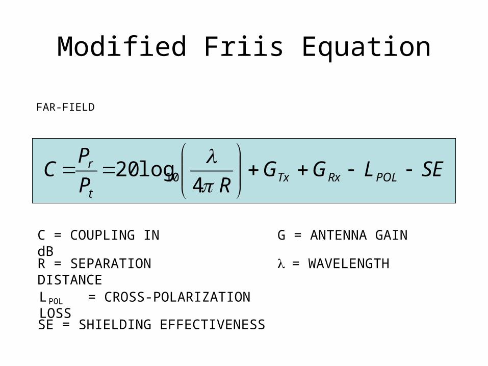
Modified Friis Equation

FAR-FIELD

C = COUPLING IN dB

R = SEPARATION DISTANCE = WAVELENGTH

G = ANTENNA GAIN

L = CROSS-POLARIZATION LOSSPOL

SE = SHIELDING EFFECTIVENESS

SELGGRP

PC POLRxTx

t

r

4log20 10

Nonlinear Effects

• Harmonic distortion

• Intermodulation distortion

• Gain Compression

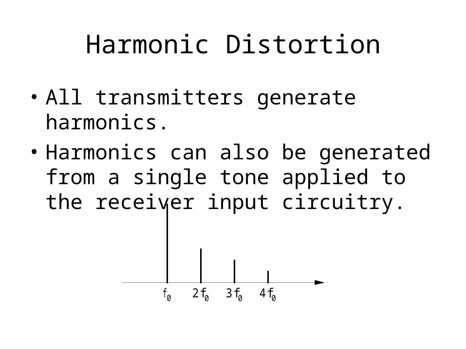
Harmonic Distortion

• All transmitters generate harmonics.

• Harmonics can also be generated from a single tone applied to the receiver input circuitry.

f0 2f0 3f0 4f0

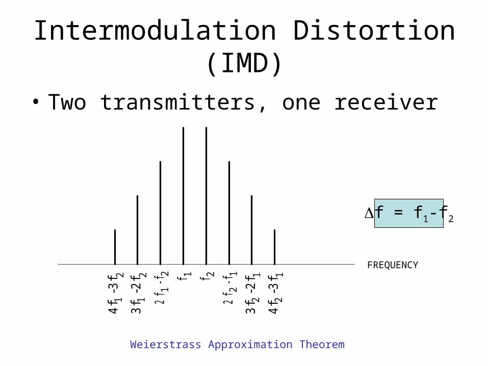
Intermodulation Distortion (IMD)

• Two transmitters, one receiver

f = f1-f2

FREQUENCY

f 1 f 2

2f -

f1

2

2f -

f2

1

3f -

2f1

2

4f -

3f1

2

3f -

2f2

1

4f -

3f2

1

Weierstrass Approximation Theorem

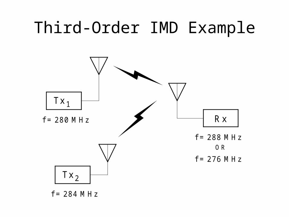
Third-Order IMD Example

Rx

Tx 1

Tx 2

f = 280 MHz

f = 284 MHz

f = 288 MHz

f = 276 MHzOR

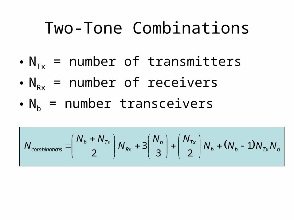
Two-Tone Combinations

• NTx = number of transmitters

• NRx = number of receivers

• Nb = number transceivers

bTxbb

TxbRx

Txbnscombinatio NNNN

NNN

NNN 1

233

2

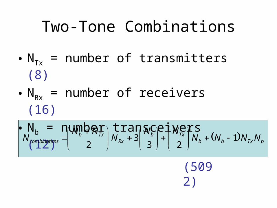
Two-Tone Combinations

• NTx = number of transmitters (8)

• NRx = number of receivers (16)

• Nb = number transceivers (12)

bTxbb

TxbRx

Txbnscombinatio NNNN

NNN

NNN 1

233

2

(5092)

Re-Radiated IMD

Tx1

Tx2

Rx1

Rx2

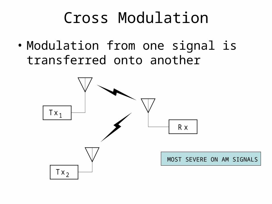
Cross Modulation

• Modulation from one signal is transferred onto another

Rx

Tx 1

Tx 2

MOST SEVERE ON AM SIGNALS

Cosite Interference Mitigation Options

• Coupling reduction• Filtering• Tuning rules• Blanking• Statistical Characterization• Active cancellation

Coupling Reduction

• Separation increase• Absorber• Cross polarization

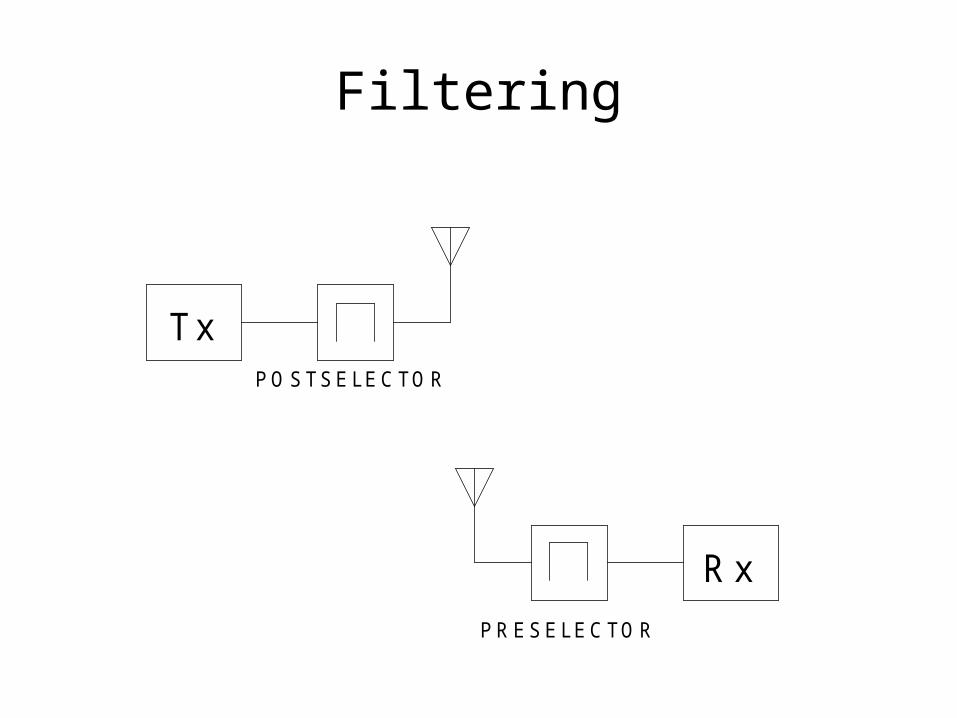
Filtering

TxPOSTSELECTOR

RxPRESELECTOR

Active Cancellation

Tx

Rx

COUPLER

AMPLITUDE &PHASE ADJUST

+

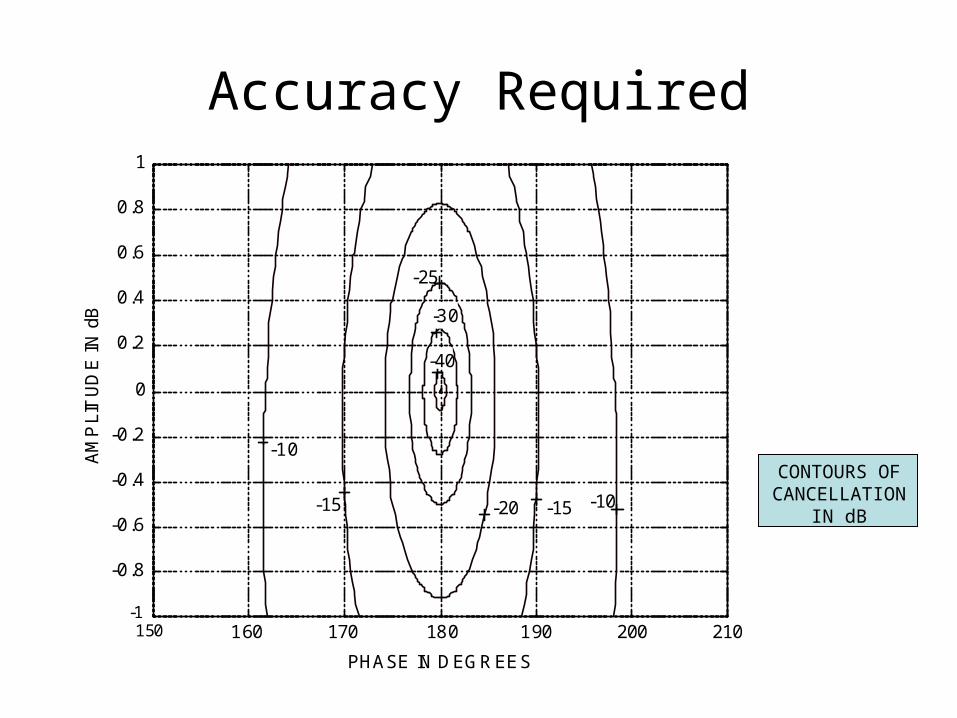
Accuracy Required

150 160 170 180 190 200 210-1

-0.8

-0.6

-0.4

-0.2

0

0.2

0.4

0.6

0.8

1

PHASE IN DEGREES

AM

PLI

TU

DE

IN

dB

-10

-15 -10 -15 -20

-25

-30

-40

CONTOURS OFCANCELLATION

IN dB

Summary

• E3 analysis is a significant portion of modern aircraft development.

• Interference from both internal and external sources must be considered for safety of flight.

• A thorough cosite interference analysis requires the evaluation of a large number of combinations.