Consequences of Cusp TrappingRob Sheldon

National Space Science & Technology Center

J. Chen, T.Fritz

Boston University

May 28, 2002

History

We discovered a high-altitude MeV electron population trapped in the cusp (GRL 98)

We also discovered diamagnetic cavities or trapped low-energy plasma in the cusp. (JGR98)

What is the relationship between high & low energy plasma? (Think rad belt & plasmasphere) Topology Waves/Energy energization

In this talk, we want to relate these two aspects of the cusp, as a possible source of rad belt MeV e-

Necessity of Quadrupolar Trap

Maxwell (~1880) showed that a perfect conductor adjacent to a dipole formed an image dipole

Chapman (~1930) realized that a neutral plasma was like a perfect conductor

Two dipoles have some quadrupole moment Therefore, every dipole embedded in a plasma,

MUST form a quadrupolar region, which is also a trap. (Nobel prize for Paul trap)

This trap is embedded in the high latitude cusp

Maxwell

Parallel Dipoles w/ ring current

-High latitude minimum, and Shabansky orbits-Bistable distributions- Quadrupolar regions of magnetosphere are important for trapping and feeding dipole.

Sheldon et al., (GRL

98) observed 1MeV

electrons at L~12,

adiabatically (but not

diffusively)

connected to the

MeV radiation belt

population. It had a

trapped, 90-degree

pitch angle

dependence.

High Latitude MinimumTrap?

The high-latitude minimum can trap a bouncing particle, which then possesses a 2nd invariant

But will the ions stay in this region, bouncing forever, or drift away? Does the 3rd invariant also exist?

The literature didn’t say, but certainly minima exist on both sides of the cusp. We did a particle tracing simulation to investigate this possibility.

Plasma Entry @ Cusps

-One magnet grounded, other biassed-Plasma generated by electrons on one magnet, feed into other trapping field due to diffusion though "x-line"-Like northward Bz, this feeding happens at the cusps-The cusps themselves hold the plasma long enough to glow, "Sheldon orbits"

But Diamagnetic Cavities?

Since this region has weak fields, trapped plasma will distort the field.

As the plasma drifts around the minimum |B|, it produces a “cusp ring current” that opposes the cusp field and makes a diamagnetic cavity.

How are these diamagnetic cavities related to the quadrupole trapped plasma? These cavities are filled with mirror mode waves and

high turbulence.

Cusp Diamagnetic Cavities

Plasma is Diamagnetic

BB BBDD

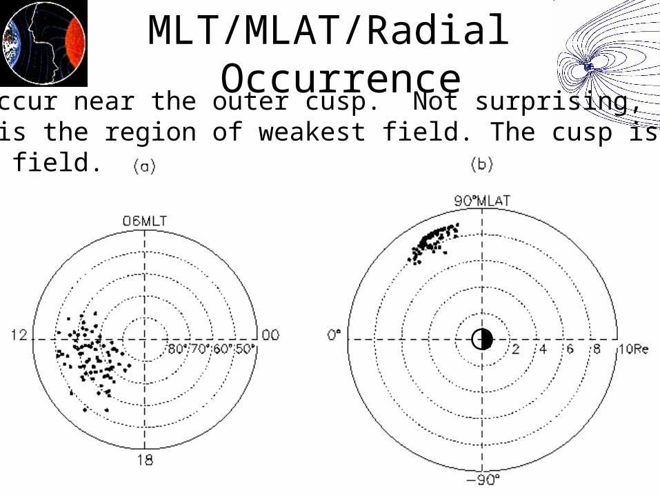
MLT/MLAT/Radial OccurrenceThe CDC occur near the outer cusp. Not surprising, becausethe cusp is the region of weakest field. The cusp is also a diverging field.

Diamagnetic Levitation

The University of Nijmegen showshow all substances are diamagnetic,and can be levitated harmlessly by the diverging (cusp-like) field in the 32mm bore of a 16 T Bitter magnet.

water drop

live frog

small frog

Stability calculation algorithm 1) Place small dipole in the cusp, anti-aligned 2) Calculate B = BDIPOLE + Bt96 for a 1 Re bubble

around the little dipole. 3) Since E=mB2 and FX = dE/dx, we repeat this

calculation for a little dx, dy, dz motion and take differences to get F. (We also get dF/dx too.)

4) Finally we adust the strength of BDIPOLE until we can get a zero force.

5) We plot these quantities to find a force free solution

Force-free dipole conditions

More Simulations

a B2

- D

6 8 r rMinimum energy found for test dipole at ~1e-8 of Earth,

placed between MP-2 Re, and MP-4 Re. Schematically, MP currents form a “hard” outer boundary, so larger CDC have centroids earthward.

Force free condition

4/800km/s, +/0/- 10nT, Day 172/294,300/10 Dst

Log scale

The Quadrupole Cusp

x x

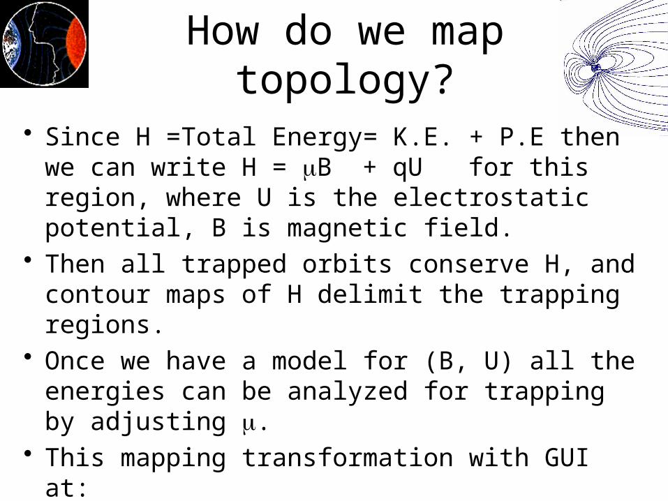
How do we map topology?

Since H =Total Energy= K.E. + P.E then we can write H = mB + qU for this region, where U is the electrostatic potential, B is magnetic field.

Then all trapped orbits conserve H, and contour maps of H delimit the trapping regions.

Once we have a model for (B, U) all the energies can be analyzed for trapping by adjusting m.

This mapping transformation with GUI at: http://cspar181.uah.edu/UBK/

http://cspar181.uah.edu/UBK

Scaling Laws

Brad ~ Bsurface= B0

Bcusp ~ B0/Rstag3

Erad= 5 MeV for Earth

Ecusp ~ v2perp~ (Bcuspr)2 ~ [(B0/Rstag

3)Rstag]

=m E/B is constant

Erad-planet~(Rstag-Earth/Rstag-planet)(B0-planet/B0-Earth)2Erad-Earth

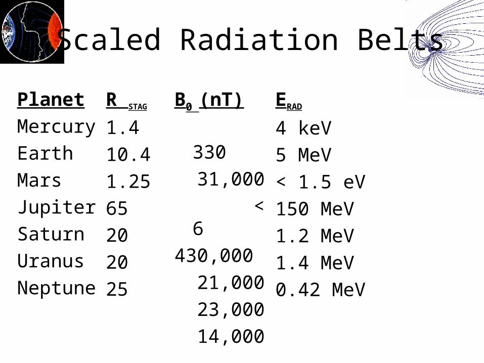
Scaled Radiation Belts

Planet

Mercury

Earth

Mars

Jupiter

Saturn

Uranus

Neptune

ERAD

4 keV

5 MeV

< 1.5 eV

150 MeV

1.2 MeV

1.4 MeV

0.42 MeV

R STAG

1.4

10.4

1.25

65

20

20

25

B0 (nT)

330

31,000

< 6

430,000

21,000

23,000

14,000

Conclusions The Cusp is a stable quadrupole trap. Diamagnetic bubbles are stable in the cusp. Non-linear relation between bubble size &

penetration into the magnetosphere These bubbles may enhance high-Energy trap. Scalings based on a Cusp accelerator produce a

reasonable estimate of Jupiter’s radiation belt energy, predict that Mars will not have a radiation belt, and lead to predictions for the other planets.

Heliosphere cusp cosmic rays?