1. IntroductionTurbulent transport of momentum, heat, water vapor and CO2 are important physical processes (Stull, 2012) in the atmospheric boundary layer (ABL). Due to computational limitation, these turbulent processes need to be parameterized in coarse-resolution weather forecast and climate models (Cohen et al., 2015; Gentine et al., 2013; Holtslag et al., 2013). Near the ground, the eddy-diffusion concept (Holtslag & Moeng, 1991; Louis, 1979; Troen & Mahrt, 1986) has been ubiquitously adopted for turbulence parameterizations.

Daytime heating of the Earth's surface causes turbulent air to transform from rolls to organized motions (Park et al., 2016; Salesky et al., 2017) due to the effects of buoyancy in the convective ABL (Agee et al., 1973), thus making it more difficult to parameterize, as convective motions generate non-local transport (i.e., non-diffusive transport (Chor et al., 2020)). To represent the non-local transport in the convective ABL, in the recent two decades, the mass-flux approach, which was originally developed for applications to cumulus convection parameterizations (Arakawa & Schubert, 1974; Bechtold et al., 2001; Betts, 1973; Tiedtke, 1989), has gained popularity in turbulence parameterization in the ABL (Angevine, 2005; Siebesma et al., 2007). In this approach, part of the turbulent flux of a scalar (e.g., potential temperature) is assumed to be trans-

Abstract Turbulence parameterizations for convective boundary layer in coarse-scale atmospheric models usually consider a combination of the eddy-diffusive transport and a non-local transport, typically in the form of a mass flux term, such as the widely adopted eddy-diffusivity mass-flux (EDMF) approach. These two types of turbulent transport are generally considered to be independent of each other. Using results from large-eddy simulations, here, we show that a Taylor series expansion of the updraft and downdraft mass-flux transport can be used to approximate the eddy-diffusivity transport in the atmospheric surface layer and the lower part of the mixed layer, connecting both eddy-diffusivity and mass-flux transport theories in convective conditions, which also quantifies departure from the Monin-Obukhov similarity (MOS) in the surface layer. This study provides a theoretical support for a unified EDMF parameterization applied to both the surface layer and mixed layer and highlights important correction required for surface models relying on MOS.

Plain Language Summary The atmospheric boundary layer is a key layer connecting the atmosphere and the surface. This boundary layer during daytime can be split into the lower surface layer where large gradients in momentum and scalars occur, overlaid by the mixed layer. In the surface layer, the concept of eddy-diffusivity transport is typically assumed and used, but it does not apply in the mixed layer, where non-local transport is essential to maintain transport under vanishing vertical gradients. These two types of transport are generally considered to be independent of each other and are usually represented in coarse-scale atmospheric models with a combination of the eddy-diffusive transport and a non-local transport, typically in the form of a mass flux term, such as the widely adopted eddy-diffusivity mass-flux (EDMF) approach. Here, we show that a Taylor series expansion of the mass-flux transport can be used to approximate the eddy-diffusivity transport in the surface layer and lower part of the mixed layer, connecting both eddy-diffusivity and mass-flux transport theories in convective conditions. This study provides a theoretical support for a unified EDMF parameterization applied to both the surface layer and mixed layer and highlights the need to account for non-local transport for Monin-Obukhov similarity-based surface-layer models.

LI ET AL.

© 2021. American Geophysical Union. All Rights Reserved.

Connection Between Mass Flux Transport and Eddy Diffusivity in Convective Atmospheric Boundary LayersQi Li1 , Yu Cheng2 , and Pierre Gentine3

1School of Civil and Environmental Engineering, Cornell University, Ithaca, NY, USA, 2Department of Earth and Planetary Sciences, Harvard University, Cambridge, MA, USA, 3Department of Earth and Environmental Engineering, Columbia University, New York, NY, USA

Key Points:• The linearized mass-flux transport

contributes to eddy-diffusivity in the surface and lower mixed layers

• This contribution quantifies departure from the Monin-Obukhov similarity scaling under increasing convective conditions

• It implies that a unified eddy-diffusivity mass-flux parameterization can be applied to both the surface and mixed layers

Supporting Information:Supporting Information may be found in the online version of this article.

Correspondence to:Q. Li,ql56@cornell.edu

Citation:Li, Q., Cheng, Y., & Gentine, P. (2021). Connection between mass flux transport and eddy diffusivity in convective atmospheric boundary layers. Geophysical Research Letters, 48, e2020GL092073. https://doi.org/10.1029/2020GL092073

Received 22 DEC 2020Accepted 20 MAR 2021

10.1029/2020GL092073RESEARCH LETTER

1 of 13

Geophysical Research Letters

ported by the mass flux associated with updraft motions (Angevine, 2005; Schumann & Moeng, 1991). Al-though details of using the mass-flux approach in ABL turbulence parameterization differ among different implementations, the general concept of this approach involves a sum of a “non-local contribution” by the mass-flux method and a “local contribution” by means of the eddy-diffusivity. For example, in Sie-besma et al.  (2007), one of the most widely adopted implementations of such eddy-diffusivity mass-flux (EDMF) approach, a profile of the turbulent eddy diffusivity that varies with the vertical distance to the surface is imposed (e.g., Equation 18 in Siebesma et al., 2007) in addition to the mass-flux transport. The EDMF approach has been implemented in many operational models, such as the ECMWF model (Köhler et al., 2011), the Navy Global Environmental Model (Sušelj et al., 2014), and National Centers for Environ-mental Prediction's (NCEP) Global Forecast System (Han et al., 2016).

However, the EDMF approach requires realistic representations of the atmospheric surface layer (ASL) that provides appropriate surface boundary conditions for obtaining the updraft characteristics, as pointed out in Witek et al. (2011). As the ASL dynamics is believed to follow the Monin-Obukhov similarity (MOS; Monin & Obukhov, 1954) scaling, the flux-gradient relationships according to the MOS functions are typi-cally invoked (e.g., Tan et al., 2018). By definition, MOS-scaling is based on an eddy-diffusivity perspective, where the turbulent flux is generated by the “local” diffusive transport mediated by turbulent eddy motions, which manifest itself in the eddy-diffusivity coefficient, K. When K is normalized with the MOS length and velocity scales (vertical distance to the surface z and friction velocity u*), it is assumed to be a function of only the stability parameter ζ = −z/L, where L is the Obukhov length.

On the other hand, increasing evidence about the impacts of large-scale coherent eddies on the non-local transport in the ASL (e.g., Khanna & Brasseur,  1997; Li et  al.,  2018; Liu et  al.,  2019; Salesky & Ander-son, 2020; Zilitinkevich et al., 2006) highlights the need to extend parameterization based on MOS beyond the local transport. Furthermore, a recent study by Chor et al. (2020) has demonstrated the importance of both local (diffusive) and non-local (caused by organized turbulent motions) throughout the convective ABL using an objective diagnostic method. In light of these new evidences, there is a need to reconcile the view points between surface-layer theory and parameterization in the mixed layer (ML). In particular, the transition region from the ASL into the ML, which is also referred to as the convective matching layer (Kaimal & Finnigan,  1994, Section 1.4.2), can be important for matching the surface fluxes with those modeled with the mass-flux approach (Randall et al., 1992), but how K departs from the MOS scaling and whether there exists a connection between mass-flux transport and eddy diffusion in this transition zone re-main largely understudied. Therefore, by analyzing the transport of potential temperature using data from large-eddy simulations (LES) of dry CBL of varying instability, we aim to examine two questions:

First, how does non-local transport due to large-scale coherent eddies impact the turbulent eddy-dif-fusivity in the surface layer? Second, how do the large-scale coherent updrafts and downdrafts modify turbulent mixing, moving from the ASL into the ML?

2. Method2.1. Flux Decomposition From Height-Dependent Tracers

To investigate the research questions, we performed three cases of LES runs (C1, C2, and C3) for dry convec-tive boundary layers, where the simulations are forced by a constant pressure gradient expressed in terms of the geostrophic wind Ug and surface heat flux 0w is imposed. Ug and 0w vary in the simulated cases, such that ASL stabilities measured by zi/L increases from case C1 to C3, where zi is the boundary layer height and L is the Obukhov length. The LES setup and numerical schemes can be found in the Supplemen-tary Information and references therein. Similar to previous studies utilizing a passive tracer to examine coherent structures (Park et al, 2016, 2017, 2018; Couvreux et al., 2010; Li et al., 2018), a height-dependent passive tracer with a constant relaxation term was simulated to aid the identification of long-range motions and the locations where updrafts and downdrafts originate from.

Before introducing the proposed method of decomposition based on the passive tracer, the notations for the flux decomposition are discussed here. The turbulent vertical flux of potential temperature is denoted as

LI ET AL.

10.1029/2020GL092073

2 of 13

Geophysical Research Letters

⟨w*θ*⟩, where ⟨⟩ represents the horizontal planar average, Z* = Z−⟨Z⟩ with Z being the vertical velocity w or the potential temperature θ. For a given horizontal plane, in this case, defined over the entire horizontal computational domain, w and θ are defined over a set E of conditions (e.g., updraft, downdraft, and envi-ronment), which can be partitioned into M mutually exclusive subsets Ei (Wang & Stevens, 2000). Invoking the law of total covariance, ⟨w*θ*⟩ can be decomposed as:

* * * *

1 1,

M M

i i i i i ii i

w w w (1)

where represents the conditional average over the subset Ei; *i iZ Z Z and i iZ Z Z , for Z being

either w or θ (See Figure 1a). It follows that 1 1Mi i . The mutually exclusive subsets are determined

from the proposed decomposition, where i  =  1, 2, and 3 corresponds to the environment, updraft, and downdraft and are denoted by i = “e,” “u,” and “d,” respectively. Thus, the entire horizontal domain has size Lx × Ly × Δz, where Lx and Ly are the horizontal dimensions of the domain and can be decomposed into the three subsets. The terms “updraft” and “downdraft” are used here in a generic way but in practice different criteria exist to classify them (as discussed in Li et al., 2018 and references therein). The first term in Equa-tion 1 can be understood mathematically as the mean of the covariance between w and θ, that is the vertical transport of potential temperature, conditioned on being an updraft (if i = 1) due to deviation of its condi-tional averaged properties from the sub-domain-averaged values (i.e., “top-hat”), which will be referred to as the within-subset Ei variability term (Wang & Stevens, 2000) hereafter. The second term is the covariance of the conditional expectations of w and θ (i.e., the “top-hat” mean Ei contribution), which will be referred to as the Ei mass-flux term hereafter. For the updraft, the second term will be the standard updraft mass-flux term. Note that Equation 1 is exact with respect to the definitions of the three mutually exclusive subsets.

LI ET AL.

10.1029/2020GL092073

3 of 13

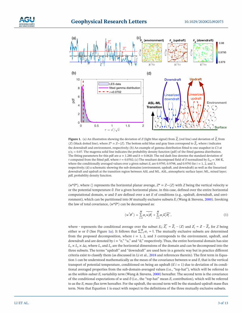
Figure 1. (a) An illustration showing the deviation of Z (light blue signal) from iZ (red line) and deviation of iZ from ⟨Z⟩ (black dotted line), where Z* = Z−⟨Z⟩. The bottom solid blue and gray lines correspond to iZ , where i indicates the downdraft and environment, respectively; (b) An example of gamma distribution fitted to one snapshot in C3 at z/zi = 0.07. The magenta solid line indicates the probability density function (pdf) of the fitted gamma distribution. The fitting parameters for this pdf are a = 1.280 and b = 0.0620. The red dash line denotes the standard deviation of τ computed from the fitted pdf, where τ = 0.0702; (c) The resultant decomposed field of θ normalized by θref = 300 K, where the conditionally averaged values over a given subset Ei are 0.9795, 0.9798, and 0.9793 for i = 1, 2, and 3, respectively; (d) a schematic showing the sub-domains (environment, updraft, and downdraft) as well as the linearized downdraft and updraft at the transition region between ASL and ML. ASL, atmospheric surface layer; ML, mixed layer; pdf, probability density function.

Geophysical Research Letters

To investigate the turbulent transition from the ASL to the ML, the proposed method for decomposing ⟨w*θ*⟩ is enabled by the height-dependent tracer s. This method successfully distinguishes the large-scale coherent structures from small-scale turbulent mixing (Davini et al., 2017; Li et al., 2018; Park et al., 2016). Here, we consider eddy time scale τ, which is the time it takes for an air parcel originating from some height z1 to reach a given height z, where 1| | /z z tke for tke being the resolved turbulent kinetic energy. The height-dependent tracer s thus enables approximating |z − z1| as |⟨s⟩−s| = s*, where s corresponds to the origins of the air parcels. The values of τ at z in the volume Lx × Ly × Δz indicate the distribution of arrival time of air parcels defined by τ. Then, a probability density function (pdf) of τ can be fitted at each height z, using a gamma distribution since the mean of τ is strictly positive (e.g., Figure 1b). The “environment” where i = 1 or “e” represents air parcels with a short arrival time, in contrast to the long-range “plumes” of updrafts and downdrafts. Thus, the “environment” is defined as the sub-domain satisfying τ ≤ σ, where σ is the standard deviation of the fitted pdf. Sub-domains of the updrafts and downdrafts follow τ > σ, where s* < 0 (s* > 0) indicates updrafts (downdrafts). Thus, any quantity of interest can be decomposed accordingly (See Figure 1c for an illustration of θ in C3).

2.2. The Linkage Between Mass Flux and Sub-Domain Variability

It is instructive to cast the general EDMF approach into the form of a conditional covariance in order to reveal the connection between mass-flux term and the within-subset variability, which will be further compared with the LES results in Section 3. For EDMF, it is usually assumed that only updrafts contribute to the mass flux transport and that the other factors (downdraft and environmental mean transport as well as the variability within each subset) can be modeled by an eddy-diffusivity approach. However, the down-draft mass flux contribution can be important (Brient et al., 2019; Davini et al., 2017; Li et al., 2018; Park et al., 2016; Wu et al., 2020) and is thus kept in our decomposition not to lose generality. Assuming that non-local turbulent transport is dominated by the mean updraft and downdraft (i.e., non-local transport) and the reminder in the environment is assumed to follow an eddy-diffusion decomposition, Equation 1 can be simplified to

1 3* * * * * * * *

1 2.i i i i i i u u u d d d

i iw w w K w w

z (2)

We will show next that this decomposition is quite accurate.

To address the first research question regarding how the mass- flux and non-local transports affect the eddy diffusivity in the surface layer, we first start with the recent results of Li et al. (2018) that the near-sur-face turbulent heat flux is a combination of both local (inner layer) turbulence and outer layer one (relat-ed to convective updrafts and downdrafts and the boundary layer; Morrison, 2007). Thus, apart from the turbulent diffusive transport contributing to ⟨w*θ*⟩ in the surface layer, contribution from the large-scale motions can be explicitly accounted for (i.e., the non-local correction) by means of the updraft and down-draft mass-flux term. Since the decomposition of ⟨w*θ*⟩ into within-subset variability and mass-flux terms is exact according to the law of total covariance, the presence of large-scale coherent motions, which do not follow the surface-layer scaling, in principle, can be written as a correction term related to the mass flux and Deardorff convective velocity (Deardorff, 1970). This is analogous to the mass-flux term in the EDMF approach, which represents the non-local contribution to heat flux (Ghannam et al., 2017; Hourdin et al., 2002; Siebesma et al., 2007). Therefore, it can be postulated and will be supported by the LES results later that the EDMF approach can be extended into the surface layer and that Equation 2 is applicable there. Using this approach one can then explicitly found the departure from Monin-Obukhov scaling due to outer layer scaling. Since in non-convective conditions the flux-gradient relationship is typically assumed MOS-scaling based on historical field data and numerical simulations (e.g., Businger et al., 1971; Kaimal et al., 1976; Khanna & Brasseur, 1997), we decompose the total flux into an eddy-diffusive part, following MOS and the mass-flux transport, which will scale with the non-local mass flux:

* * ,MOS u u d dw K M M

z (3)

LI ET AL.

10.1029/2020GL092073

4 of 13

Geophysical Research Letters

where KMOS is the eddy-diffusivity that follows MOS, that is wall-bounded scaling and *( )i i i i iM w w w , the mass flux transport, where i indicates either updraft (u) or downdraft (d).

Close to the wall, within the surface layer, the term u involved in the mass-flux transport in Equation 3 can be seen as a positive temperature anomaly associated with an air parcel rising (i.e., updraft motion) from a distance lu below some reference level z. This positive anomaly in θ is transported by the updraft from z − lu to the reference level z. lu is commensurate with the vertical length scale of turbulent eddy responsible for the transport (Corrsin, 1975; Priestley & Swinbank, 1947; Raupach, 1987). The mass-flux contribution to turbulent heat flux is associated with convective turbulence (Priestley & Swinbank, 1947), in addition to the down-gradient mechanical turbulent component as proposed by Priestley and Swinbank (1947) based on the classic Prandtl's mixing-length argument (Bradshaw, 1974; Prandtl, 1925). For downdraft, we may also suppose the same condition holds and d is the negative anomaly in θ associated with an air parcel identified as downdraft compared to its average θ at z + ld. Therefore, using a Taylor series expansion around z to approximate the temperature anomalies, Equation 3 can be written as:

* * ( , ),MOS u u d d u dw K l M l M HOT l l

z (4)

provided lu and ld are small compared to the length scale for a change in d⟨θ⟩/dz (Corrsin,  1975; Rau-pach, 1987), where HOT(lu, ld) refers to the higher order terms. Equation 4 indicates that the total effective turbulent eddy diffusivity can be attributed to both an eddy diffusion following the standard MOS-scaling and a contribution from the non-local mass-flux transport generating a new eddy diffusion term. Indeed, the terms in the Taylor series expansion that are linear in lu and ld explicitly contribute to the total eddy diffusivity:

,linear u u d dMF l M l M

z (5)

where MFlinear is the linearized mass-flux transport. Essentially, near the surface, the mass-flux transport acts as a correction to KMOS, but moving up from the ASL, the approximation of the mass flux contribution by the local gradient in the Taylor series expansion becomes invalid because d⟨θ⟩/dz approaches zero. Yet to apply such linearization to obtain the gradient-diffusion relationship, the vertical length scale of the turbulence effecting the transfer needs to be much smaller than the length scale for a change of d⟨θ⟩/dz with height, according to discussions about the validity of gradient-diffusion hypothesis in Corrsin (1975); Raupach (1987). This criterion thus defines regimes of applicability of this expansion.

Next, to facilitate subsequent discussions, we define explicitly the eddy diffusivities K and the Monin-Obuk-hov stability correction functions for potential temperature ϕh according to the flux-gradient relationship. First, according to Equation 5,

.mf u u d dK l M l M (6)

KMOS can be approximated according to Equation 4 as

* *.linear

MOSw MFK

z (7)

Considering the sum of the within-subset variability, Kvar is defined as:

,i i i ivar

wK

z (8)

and similarly, if only the environmental variability is considered, its associated eddy diffusivity Kenv is

LI ET AL.

10.1029/2020GL092073

5 of 13

Geophysical Research Letters

.e e eenv

wK

z (9)

Using the definition of

*h

z dT dz

, where * */sT w u , for sw being the surface kinematic heat flux,

it can be shown that ih, the Monin-Obukhov stability correction function corresponding to different Ki as

defined in Equations 6–9 is given by

* ,/

sih h

i i

w zuK d dz K

(10)

where i refers to “mf,” “MOS,” “var,” and “env.”

3. Results and Discussion3.1. Turbulent Flux Decomposition From LES

We first examine the quantities derived in Section 2 based on the mass-flux decomposition and how they vary vertically in the boundary layer as a function of stability. The demarcation between the ASL and ML is taken to be 0.1zi based on the commonly adopted assumption that the ASL depth is about 10% of the boundary layer height (Wyngaard, 2010, Chapter 11). The values of αi shown in Figure 2a indicate area fractions of the three types of sub-domains. Below z/zi = 0.3, αe, the environment dominates and it

LI ET AL.

10.1029/2020GL092073

6 of 13

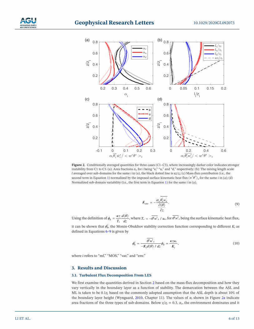
Figure 2. Conditionally averaged quantities for three cases (C1–C3), where increasingly darker color indicates stronger instability from C1 to C3. (a): Area fractions αi, for i being “e,” “u,” and “d,” respectively; (b): The mixing length scale l averaged over sub-domains for the same i in (a), the black dotted line is κz/zi; (c) Mass-flux contribution (i.e., the second term in Equation 1) normalized by the imposed surface kinematic heat flux * *

sw for the same i in (a); (d) Normalized sub-domain variability (i.e., the first term in Equation 1) for the same i in (a).

0.2 0.3 0.4 0.5 0.6

i

0.2

0.4

0.6

0.8

z/z i

0 0.05 0.1 0.15 0.2

li/z

i

0.2

0.4

0.6

0.8

z/z i

-0.1 0 0.1 0.2 0.3

0.2

0.4

0.6

0.8

z/z i

eud

0 0.2 0.4 0.6

0.2

0.4

0.6

0.8

z/z i

(a) (b)

(c) (d)

Geophysical Research Letters

decreases with increasing instability, which physically means that large-scale coherent motions become more prevalent. However, with an increasing instability, αu increases especially in the surface layer and lower part of the ML, but both αd and αu decrease as they approach the surface. It is worth noting that αd does not vary significantly with stability condition for z/zi < 0.8 and it exceeds the area fractions of the updraft and the environment in the ML. The resultant partitioning in this study is different from the results obtained in Chinita et al. (2018), where the joint probability density of vertical velocity and scalars are partitioned into a joint Gaussian part and the complement, representing the local turbulent mixing and the large-scale coherent motions, respectively. The difference likely results from partitioning criterion for the environment subset, in which a joint-Gaussian distribution is imposed in Chinita et al. (2018), but our current decomposition criterion leads to a non-Gaussian joint distribution in the environment subset (results not shown). Future studies are needed to further investigate this point, which is beyond the scope of this paper.

The values of l are defined using the height-dependent tracer s, where *i il s , indicating the average length

scale of mixing, depending on where the air parcels originate from. The vertical profiles of l (Figure 2b) show that le is an order of magnitude smaller than ld and lu, the updraft and downdraft mixing lengths, further confirming the hypothesis that the environment can be treated as a localized mixing. For z/zi ≤ 0.2, ld > lu and lu approaches κz (dotted line in Figure 2b), the distance to the wall scaling, as instability decreas-es. On the other hand, above z/zi ≈ 0.4, ld slightly decreases toward a similar value as that near surface while lu approaches a constant value lu ≈ 0.12zi. The increasing discrepancy between ld and lu for z/zi ≤ 0.4 indicates asymmetry in the mixing lengths associated with updraft and downdraft.

The different terms in Equation 1 are analyzed in Figures 2c and 2d, which are averaged over one eddy turn-over time Teto = zi/w* and normalized by the prescribed surface kinematic heat flux. As for

* *i i iw shown

in Figure 2c, the environment mass-flux term is insignificant since the mass flux Me (not shown here) is close to zero. In contrast, the updraft and downdraft dominate the mass-flux transport. In addition, the updraft contribution increases as instability increases near the wall, resulting from buoyant thermals with

large temperature and vertical velocity anomalies (Hourdin et al., 2002). As for i i iw (Figure 2d), the envi-

ronment component clearly dominates and is the largest contribution to the the total flux in the surface lay-er and lower part of the ML, for example, z/zi < 0.2 for the most convective case, reaching a range between

40% and 60%. It is also worth noting that d d dw is negligible compared to the updraft counterpart. Thus,

the updraft subset variability u u uw can be of similar magnitude as the updraft mass-flux term

* *u u uw ,

especially for C3, the most convective case, which is an indication of localized mixing due to small-scale ed-dies in the updraft sub-domain and is consistent with the eddy-diffusion hypothesis used in previous studies (Ghannam et al., 2017; Hourdin et al., 2002).

3.2. Non-Local Mass-Flux Contribution to Departure From MOS

The flux-gradient relationships in the ASL typically assume that the eddy diffusivity K is only a function of z/L according to MOS-scaling. As discussed in the Introduction, there has been increasing evidence of an outer layer influence (i.e., z/zi as an additional length scale) under more convective conditions, which may explain the departure from the MOS-scaling. Thus, in this section, the LES results will be analyzed to demonstrate how z/zi scaling arises in the surface layer through the connection with the non-local mass-flux transport (e.g., Equation 4).

The stability correction functions ih corresponding to each of the turbulent eddy diffusivities Ki (Equation 6

and Equation 7) are shown in Figure 3 according to

*i

h

zuK . First, for all three cases, distinct behav-

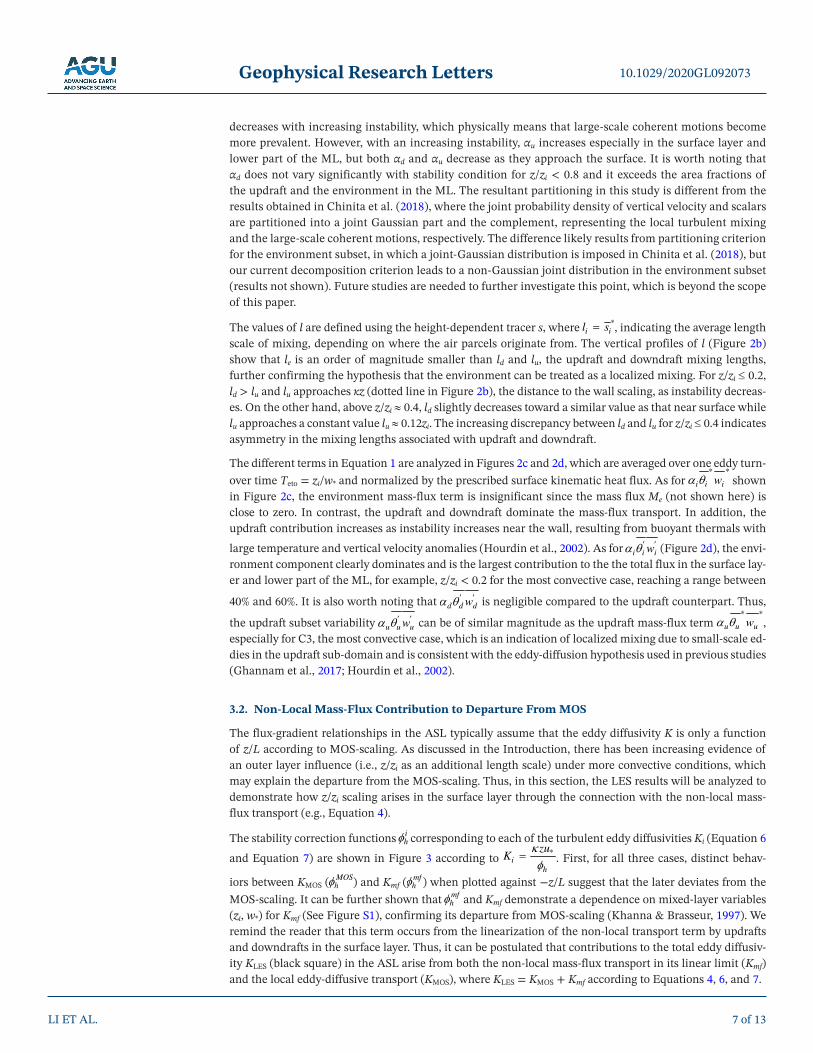
iors between KMOS (MOSh ) and Kmf (mf

h ) when plotted against −z/L suggest that the later deviates from the MOS-scaling. It can be further shown that mf

h and Kmf demonstrate a dependence on mixed-layer variables (zi, w*) for Kmf (See Figure S1), confirming its departure from MOS-scaling (Khanna & Brasseur, 1997). We remind the reader that this term occurs from the linearization of the non-local transport term by updrafts and downdrafts in the surface layer. Thus, it can be postulated that contributions to the total eddy diffusiv-ity KLES (black square) in the ASL arise from both the non-local mass-flux transport in its linear limit (Kmf) and the local eddy-diffusive transport (KMOS), where KLES = KMOS + Kmf according to Equations 4, 6, and 7.

LI ET AL.

10.1029/2020GL092073

7 of 13

Geophysical Research Letters

In addition, the solid line denotes the Businger-Dyer (BD) similarity function (Businger, 1966), which is one of the most widely adopted empirical functional forms of ϕh. Within a simulation, the values of LES

h and KLES (black square in Figure 3) deviate from BD

h , the Businger-Dyer (BD) similarity function, but the overall trend follows the MOS-scaling, which is consistent with previous findings from LES and direct numerical simulation results (Li et al., 2018; Maronga & Reuder, 2017; Pirozzoli et al., 2017). Although some differenc-es between MOS

h and BDh are found within the cluster of points in C1 and C2, importantly, MOS

h and KMOS (Equation 6, open circles in Figure 3) vary with the MOS stability parameter −z/L since a decreasing trend spanning three decades of −z/L is observed, unlike the lack of dependence on −z/L for mf

h and Kmf (Khanna & Brasseur, 1997). Overall, different scaling behaviors of KMOS and Kmf shown in Figure 3 suggest that the local environmental eddy diffusion and the influence of the non-local transport in the ASL can be unified by considering the impact of mass-flux transport as a new, additional eddy diffusion in its linear limit.

Furthermore, values of Kvar (Equation 8) and Kenv (Equation 9) as well as the corresponding ϕhs are shown in Figure S2. For cases C1 and C2, a good agreement between Kvar, Kenv and KMOS further demonstrates that the mass-flux transport effective approaches its linear limit as Kmf according to Equation 4. However, Kvar and Kenv in C3 deviate from the MOS-scaling, suggesting that large-scale eddies increasingly influence turbulent mixing near surface that give rise to the within-subset variability. Interestingly, the similarity between Kenv and Kmf indicates a possible connection between the mass-flux and the within-subset variability terms in the EDMF approach. The implications of this perspective on turbulent eddy diffusivity as the ASL transitions into the ML will be examined in the next section.

3.3. The Role of Linearized Mass-Flux Term in the ASL-ML Transition

In general, in the EDMF approach (e.g., Siebesma et  al.,  2007) or the eddy diffusivity counter-gradient approach (e.g., Deardorff, 1966; Holtslag & Moeng, 1991), the eddy diffusivity K needs to be parameter-ized to represent the local (diffusive) transport. For instance, K can be derived from subtracting the mod-eled non-local (counter-gradient) transport from the total turbulent flux (Holtslag & Moeng,  1991) and more recently from an optimization approach by maximizing diffusive transport for a passive scalar (Chor et al., 2020). Matching of K with the prediction based on the MOS-scaling near top of the ASL (typically z/zi ≈ 0.1) is usually ensured by directly imposing the surface similarity function (Troen & Mahrt, 1986) or making sure that the local free-convection limit 4 /3( / )iz z in the ASL can be recovered, for example in the profile of K applied in the EDMF approach (Equation 11; Siebesma et al., 2007, Equation 18) based on Holtslag and Moeng (1991). Figures 4a–4c compare the eddy diffusivity computed from the decomposed turbulent fluxes based on LES data and KHoltslag according to Siebesma et al. (2007, Equation 18), where

LI ET AL.

10.1029/2020GL092073

8 of 13

Figure 3. The Monin-Obukhov stability correction function ih (a) corresponding to different Ki and (b) the normalized

eddy diffusivity coefficient *

Kzu

plotted against the stability parameter −z/L, where different Ks and ϕhs are defined in

Equations 6–10 and KLES/κzu* = −⟨w*θ*⟩/(d⟨θ⟩/dz) =  1 / LESh . The three clusters of points are plotted with increasing

−z/L, corresponding to cases C1, C2, and C3, respectively. Solid line indicates the Businger-Dyer similarity function 1/2(1 16 / )BD

h z L . The LES data are plotted for 0.03 < z/zi ≤ 0.1. Note that for better visual effect, the markers are not plotted at each level of the LES data.

Geophysical Research Letters

1/32 231 *

* 0 **

1 39 1 .Holtslag i h ii i i i i

z z u z z zK z u z wz z w z z z

(11)

The eddy diffusivity Kvar (Equation 8) is close to KHoltslag in the ASL and the lower part of the ML (i.e., z/zi ≤ 0.2). For cases C2 and C3, the agreements are better compared to that in Figure 4a. This might be re-lated to the fact that the stability correction function ϕh0 = (1 − 39z/L)−1/3 in Equation 11 follows the local free-convective scaling (Maronga & Reuder, 2017). For the upper ML near temperature inversion (0.5 < z/zi ≤ 0.8) (i.e., away from vanishing gradients as there the diffusion is ill-posed), a good agreement between Kvar and KHoltslag is also observed in Figures 4a–4c. This further confirms that the height-dependent trac-er-based decomposition is a robust method to separate the subset variability term from the total turbulent flux for the lower part of the mixed layer before d⟨θ⟩/dz approaches zero, which can be modeled as diffusive transport with an eddy diffusivity derived from the counter-gradient eddy diffusion approach (Holtslag & Moeng, 1991).

In addition, for z/zi ≤ 0.2 (especially C2 and C3), Kmf associated with the linearized mass-flux transport nicely matches Kenv, which is the eddy diffusivity associated with the environment subset variability (Equa-tion 9; See Figures 4d–4f). This suggests that Kenv in the ASL-ML transition region can be approximated by Kmf, especially for increasingly convective cases C2 and C3 (i.e., u*/w* ≤ 0.3). Therefore, this leads to a decomposition of ⟨w*θ*⟩ in the lower part of the ML as:

LI ET AL.

10.1029/2020GL092073

9 of 13

Figure 4. (a)–(c):Kvar (Equation 8) in comparison with the expression in Holtslag and Moeng (1991). (d)–(f) Kenv (Equation 9) and Kmf (Equation 6) normalized by w* and zi.

0 0.1 0.2

0.2

0.4

0.6

0.8

C1

0 0.1 0.2

0.2

0.4

0.6

0.8

C1

0 0.1 0.2

0.2

0.4

0.6

0.8

C2

0 0.1 0.2

0.2

0.4

0.6

0.8

C2

0 0.1 0.2

0.2

0.4

0.6

0.8

C3

Kmf

Kenv

0 0.1 0.2

0.2

0.4

0.6

0.8

C3

K (Holtslag)Kvar

(a) (b) (c)

(d) (e) (f)

Geophysical Research Letters

w Kz

M M

l M l Mz

u u d d

u u d d

* *

MM Mu u d d , (12)

where γ is a constant of order one.

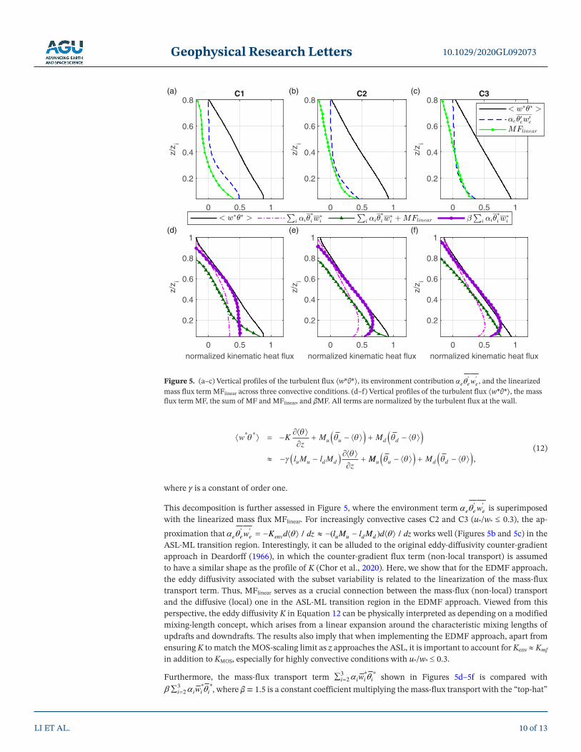
This decomposition is further assessed in Figure 5, where the environment term e e ew is superimposed

with the linearized mass flux MFlinear. For increasingly convective cases C2 and C3 (u*/w* ≤ 0.3), the ap-

proximation that / ( ) /e e e env u u d dw K d dz l M l M d dz works well (Figures 5b and 5c) in the ASL-ML transition region. Interestingly, it can be alluded to the original eddy-diffusivity counter-gradient approach in Deardorff  (1966), in which the counter-gradient flux term (non-local transport) is assumed to have a similar shape as the profile of K (Chor et al., 2020). Here, we show that for the EDMF approach, the eddy diffusivity associated with the subset variability is related to the linearization of the mass-flux transport term. Thus, MFlinear serves as a crucial connection between the mass-flux (non-local) transport and the diffusive (local) one in the ASL-ML transition region in the EDMF approach. Viewed from this perspective, the eddy diffusivity K in Equation 12 can be physically interpreted as depending on a modified mixing-length concept, which arises from a linear expansion around the characteristic mixing lengths of updrafts and downdrafts. The results also imply that when implementing the EDMF approach, apart from ensuring K to match the MOS-scaling limit as z approaches the ASL, it is important to account for Kenv ≈ Kmf in addition to KMOS, especially for highly convective conditions with u*/w* ≤ 0.3.

Furthermore, the mass-flux transport term 3 * *2i i i iw shown in Figures  5d–5f is compared with

3 * *2i i i iw , where β = 1.5 is a constant coefficient multiplying the mass-flux transport with the “top-hat”

LI ET AL.

10.1029/2020GL092073

10 of 13

Figure 5. (a–c) Vertical profiles of the turbulent flux ⟨w*θ*⟩, its environment contribution e e ew , and the linearized

mass flux term MFlinear across three convective conditions. (d–f) Vertical profiles of the turbulent flux ⟨w*θ*⟩, the mass flux term MF, the sum of MF and MFlinear, and βMF. All terms are normalized by the turbulent flux at the wall.

0 0.5 1

0.2

0.4

0.6

0.8

z/z i

C1

0 0.5 1normalized kinematic heat flux

0.2

0.4

0.6

0.8

1

z/z i

0 0.5 1

0.2

0.4

0.6

0.8

z/z i

C2

0 0.5 1normalized kinematic heat flux

0.2

0.4

0.6

0.8

1

z/z i

0 0.5 1

0.2

0.4

0.6

0.8

z/z i

C3

0 0.5 1normalized kinematic heat flux

0.2

0.4

0.6

0.8

1

z/z i

(a) (b) (c)

(d) (e) (f)

Geophysical Research Letters

assumption. The value of β = 1.5 has been shown by LES results to correctly predict for z/zi > 0.1 as dis-cussed in previous studies (Petersen et al., 1999; Schumann & Moeng, 1991). However, 3 * *

2i i i iw de-creases near the ASL, indicating that the eddy-diffusive transport is missing from this formulation. Hence, adding MFlinear to the mass-flux transport term accounts for the environment subset variability, which can be modeled as an eddy-diffusive transport in the lower part of the ML (line with triangles in Figures 5d–5f). The value of γ in Equation 12 averaged over z where d⟨θ⟩/dz is non-vanishing ranges from 1.35 (C3) to 1.48 (C1), which is of order one. Thus, the connections between eddy diffusion and mass-flux transport in the EDMF approach can be summarized: first, for less convective case in the ASL (e.g., C1) or close to the surface (e.g., C2; c.f., Equation 4), Kmf is a good approximation of the mass-flux transport; second, with increasing instability (e.g., C2 and C3), the linearized mass-flux transport (c.f. Figures 5b and 5c) is closely related to Kenv, which contributes to the eddy-diffusive transport, in addition to the typical “top-hat” mean mass-flux transport.

4. ConclusionIn this paper, we show by decomposition of turbulent vertical potential temperature fluxes in LES results and analytical derivation that the connection between the mass-flux and eddy-diffusion in the EDMF framework is important to understand the departure of eddy diffusivity from the MOS scaling in the surface layer as well as informing a unified treatment of the ASL and ML. The turbulent flow field of the simulated dry convective ABL is divided into three sub-domains: the environment, updrafts, and downdrafts by track-ing height-dependent tracers. In each sub-domain, the turbulent scalar flux ⟨w*θ*⟩ is decomposed into the

sub-domain variability i iw (eddy-diffusivity type) and mass-flux contribution * *

i iw . From analyzing the decomposed fluxes and the associated turbulent eddy diffusivities, we examine the two proposed questions, in which the following two main points can be made:

1. In the ASL, the first-order derivative term in a Taylor series expansion of the non-local mass-flux trans-port can be regarded as a non-local contribution to the ASL eddy diffusivity generating deviation from the Monin-Obukhov scaling. Thus, in the EDMF approach, there is a natural linkage between eddy-dif-fusivity and mass-flux transport in the ASL

2. As the ASL transitions into the ML under increasingly convective conditions (u*/w* ≤ 0.3), the linearized

mass flux MFlinear is a good approximation to the environment term e e ew , which is modeled as the

eddy-diffusive turbulent transport in the EDMF approach

The effect of mass-flux transport can be incorporated into the eddy diffusivity near surface to scale as a func-tion of both local stability (scaling with the distance to the wall) and the boundary layer stability (scaling with the depth of the boundary layer). Hence, we conclude that a unified approach to turbulence employing a general EDMF approach with updrafts and downdrafts can be deployed into the surface layer, instead of treating turbulence in the ASL as a separate boundary condition. This has the additional advantage to ex-plicitly represent the non-local transport departure from Monin-Obukhov near the surface, which is absent in current generation of land and atmosphere surface models yet appears critical especially in convective conditions.

Data Availability StatementData are available from https://doi.org/10.7298/01dd-wq90.

ReferencesAgee, E. M., Chen, T. S., & Dowell, K. E. (1973). A review of mesoscale cellular convection. Bulletin of the American Meteorological Society,

54(10), 1004–1012. https://doi.org/10.1175/1520-0477(1973)054<1004:aromcc>2.0.co;2Angevine, W. M. (2005). An integrated turbulence scheme for boundary layers with shallow cumulus applied to pollutant transport. Jour-

nal of Applied Meteorology, 44(9), 1436–1452. https://doi.org/10.1175/jam2284.1Arakawa, A., & Schubert, W. H. (1974). Interaction of a cumulus cloud ensemble with the large-scale environment, part I. Journal of the

Atmospheric Sciences, 31(3), 674–701. https://doi.org/10.1175/1520-0469(1974)031<0674:ioacce>2.0.co;2Bechtold, P., Bazile, E., Guichard, F., Mascart, P., & Richard, E. (2001). A mass-flux convection scheme for regional and global models.

Quarterly Journal of the Royal Meteorological Society, 127(573), 869–886. https://doi.org/10.1002/qj.49712757309

LI ET AL.

10.1029/2020GL092073

11 of 13

AcknowledgmentsP. Gentine would like to acknowledge funding from the National Science Foundation (NSF CAREER, EAR- 1552304) and from the Department of Energy (DOE Early Career, DE-SC00142013). The simulations were performed on the computing clusters of the National Center of Atmospheric Research under Project UCLB0017. Q. Li would like to acknowledge funding from the National Science Foundation (NSF-AGS 2028644 and NSF-CBET 2028842) and the computational resources provided by Cheyenne by the National Center for Atmospheric Research (UCOR00029).

Geophysical Research Letters

Betts, A. K. (1973). Non-precipitating cumulus convection and its parameterization. Quarterly Journal of the Royal Meteorological Society, 99(419), 178–196. https://doi.org/10.1002/qj.49709941915

Bradshaw, P. (1974). Possible origin of Prandt's mixing-length theory. Nature, 249, 135. https://doi.org/10.1038/249135b0Brient, F., Couvreux, F., Villefranque, N., Rio, C., & Honnert, R. (2019). Object-oriented identification of coherent structures in

large eddy simulations: Importance of downdrafts in stratocumulus. Geophysical Research Letters, 46(5), 2854–2864. https://doi.org/10.1029/2018gl081499

Businger, J. (1966). Transfer of heat and momentum in the atmospheric boundary layer. In Proc. arctic heat budget and atmospheric circu-lation (pp. 305–332).

Businger, J. A., Wyngaard, J. C., Izumi, Y., & Bradley, E. F. (1971). Flux-profile relationships in the atmospheric surface layer. Journal of the Atmospheric Sciences, 28(2), 181–189. https://doi.org/10.1175/1520-0469(1971)028<0181:fprita>2.0.co;2

Chinita, M. J., Matheou, G., & Teixeira, J. (2018). A joint probability density-based decomposition of turbulence in the atmospheric bound-ary layer. Monthly Weather Review, 146(2), 503–523. https://doi.org/10.1175/mwr-d-17-0166.1

Chor, T., McWilliams, J. C., & Chamecki, M. (2020). Diffusive-nondiffusive flux decompositions in atmospheric boundary layers. Journal of the Atmospheric Sciences, 77(10), 3479–3494. https://doi.org/10.1175/jas-d-20-0093.1

Cohen, A. E., Cavallo, S. M., Coniglio, M. C., & Brooks, H. E. (2015). A review of planetary boundary layer parameterization schemes and their sensitivity in simulating southeastern U.S. cold season severe weather environments. Weather and Forecasting, 30(3), 591–612. https://doi.org/10.1175/waf-d-14-00105.1

Corrsin, S. (1975). Limitations of gradient transport models in random walks and in turbulence. Advances in Geophysics, 18, 25–60. https://doi.org/10.1016/s0065-2687(08)60451-3

Couvreux, F., Hourdin, F., & Rio, C. (2010). Resolved versus parametrized boundary-layer plumes. part I: A parametrization-oriented con-ditional sampling in large-eddy simulations. Boundary-Layer Meteorology, 134(3), 441–458. https://doi.org/10.1007/s10546-009-9456-5

Davini, P., D'Andrea, F., Park, S.-B., & Gentine, P. (2017). Coherent structures in large-eddy simulations of a nonprecipitating stratocumu-lus-topped boundary layer. Journal of the Atmospheric Sciences, 74(12), 4117–4137. https://doi.org/10.1175/jas-d-17-0050.1

Deardorff, J. W. (1966). The counter-gradient heat flux in the lower atmosphere and in the laboratory. Journal of the Atmospheric Sciences, 23(5), 503–506. https://doi.org/10.1175/1520-0469(1966)023<0503:tcghfi>2.0.co;2

Deardorff, J. W. (1970). Convective velocity and temperature scales for the unstable planetary boundary layer and for rayleigh convection. Journal of the Atmospheric Sciences, 27(8), 1211–1213. https://doi.org/10.1175/1520-0469(1970)027<1211:cvatsf>2.0.co;2

Gentine, P., Holtslag, A. A. M., D'Andrea, F., & Ek, M. (2013). Surface and atmospheric controls on the onset of moist convection over land. Journal of Hydrometeorology, 14(5), 1443–1462. https://doi.org/10.1175/jhm-d-12-0137.1

Ghannam, K., Duman, T., Salesky, S. T., Chamecki, M., & Katul, G. (2017). The non-local character of turbulence asymmetry in the con-vective atmospheric boundary layer. Quarterly Journal of the Royal Meteorological Society, 143(702), 494–507. https://doi.org/10.1002/qj.2937

Han, J., Witek, M. L., Teixeira, J., Sun, R., Pan, H.-L., Fletcher, J. K., & Bretherton, C. S. (2016). Implementation in the NCEP GFS of a hybrid eddy-diffusivity mass-flux (EDMF) boundary layer parameterization with dissipative heating and modified stable boundary layer mixing. Weather and Forecasting, 31(1), 341–352. https://doi.org/10.1175/waf-d-15-0053.1

Holtslag, A. A. M., & Moeng, C.-H. (1991). Eddy diffusivity and countergradient transport in the convective atmospheric boundary layer. Journal of the Atmospheric Sciences, 48(14), 1690–1698. https://doi.org/10.1175/1520-0469(1991)048<1690:edacti>2.0.co;2

Holtslag, A. A. M., Svensson, G., Baas, P., Basu, S., Beare, B., Beljaars, A. C. M., et al.(2013). Stable atmospheric boundary layers and diur-nal cycles: challenges for weather and climate models. Bulletin of the American Meteorological Society, 94(11), 1691–1706. https://doi.org/10.1175/bams-d-11-00187.1

Hourdin, F., Couvreux, F., & Menut, L. (2002). Parameterization of the dry convective boundary layer based on a mass flux representation of thermals. Journal of the Atmospheric Sciences, 59(6), 1105–1123. https://doi.org/10.1175/1520-0469(2002)059<1105:potdcb>2.0.co;2

Kaimal, J., & Finnigan, J. (1994). Atmospheric boundary layer flows: Their structure and measurement. Oxford University PressKaimal, J. C., Wyngaard, J. C., Haugen, D. A., Coté, O. R., Izumi, Y., Caughey, S. J., & Readings, C. J. (1976). Turbulence structure in the convective

boundary layer. Journal of the Atmospheric Sciences, 33(11), 2152–2169. https://doi.org/10.1175/1520-0469(1976)033<2152:tsitcb>2.0.co;2Khanna, S., & Brasseur, J. G. (1997). Analysis of Monin-Obukhov similarity from large-eddy simulation. Journal of Fluid Mechanics, 345,

251–286. https://doi.org/10.1017/s0022112097006277Köhler, M., Ahlgrimm, M., & Beljaars, A. (2011). Unified treatment of dry convective and stratocumulus-topped boundary layers in the

ECMWF model. Quarterly Journal of the Royal Meteorological Society, 137(654), 43–57. https://doi.org/10.1002/qj.713Li, Q., Gentine, P., Mellado, J. P., & McColl, K. A. (2018). Implications of nonlocal transport and conditionally averaged statistics on

Monin-Obukhov similarity theory and townsend's attached eddy hypothesis. Journal of the Atmospheric Sciences, 75(10), 3403–3431. https://doi.org/10.1175/jas-d-17-0301.1

Liu, S., Zeng, X., Dai, Y., & Shao, Y. (2019). Further improvement of surface flux estimation in the unstable surface layer based on large-ed-dy simulation data. Journal of Geophysical Research: Atmospheres, 124(17–18), 9839–9854. https://doi.org/10.1029/2018jd030222

Louis, J.-F. o. (1979). A parametric model of vertical eddy fluxes in the atmosphere. Boundary-Layer Meteorology, 17(2), 187–202. https://doi.org/10.1007/bf00117978

Maronga, B., & Reuder, J. (2017). On the formulation and universality of Monin-Obukhov similarity functions for mean gradients and standard deviations in the unstable surface layer: Results from surface-layer-resolving large-eddy simulations. Journal of the Atmospher-ic Sciences, 74(4), 989–1010. https://doi.org/10.1175/jas-d-16-0186.1

Monin, A. S., & Obukhov, A. M. (1954). Basic laws of turbulent mixing in the surface layer of the atmosphere. Contributions to Geophysical Institute of the Academy of Sciences of the USSR, 151(163), e187

Morrison, J. F. (2007). The interaction between inner and outer regions of turbulent wall-bounded flow. Philosophical Transactions of the Royal Society A, 365(1852), 683–698. https://doi.org/10.1098/rsta.2006.1947

Park, S.-B., Böing, S., & Gentine, P. (2018). Role of surface friction on shallow nonprecipitating convection. Journal of the Atmospheric Sciences, 75(1), 163–178. https://doi.org/10.1175/jas-d-17-0106.1

Park, S.-B., Gentine, P., Schneider, K., & Farge, M. (2016). Coherent structures in the boundary and cloud layers: Role of updrafts, subsiding shells, and environmental subsidence. Journal of the Atmospheric Sciences, 73(4), 1789–1814. https://doi.org/10.1175/jas-d-15-0240.1

Park, S.-B., Heus, T., & Gentine, P. (2017). Role of convective mixing and evaporative cooling in shallow convection. Journal of Geophysical Research: Atmospheres, 122(10), 5351–5363. https://doi.org/10.1002/2017jd026466

Petersen, A. C., Beets, C., van Dop, H., Duynkerke, P. G., & Siebesma, A. P. (1999). Mass-flux characteristics of reactive scalars in the convective boundary layer. Journal of the Atmospheric Sciences, 56(1), 37–56. https://doi.org/10.1175/1520-0469(1999)056<0037:mfcors>2.0.co;2

LI ET AL.

10.1029/2020GL092073

12 of 13

Geophysical Research Letters

Pirozzoli, S., Bernardini, M., Verzicco, R., & Orlandi, P. (2017). Mixed convection in turbulent channels with unstable stratification. Jour-nal of Fluid Mechanics, 821, 482. https://doi.org/10.1017/jfm.2017.216

Prandtl, L. (1925). 7. Bericht über Untersuchungen zur ausgebildeten Turbulenz. Zeitschrift für Angewandte Mathematik und Mechanik, 5, 136–139. https://doi.org/10.1002/zamm.19250050212

Priestley, C. H. B., & Swinbank, W. C. (1947). Vertical transport of heat by turbulence in the atmosphere. Proceedings of the Royal Society of London–Series A: Mathematical and Physical Sciences, 189(1019), 543–561.

Randall, D. A., Shao, Q., & Moeng, C.-H. (1992). A second-order bulk boundary-layer model. Journal of the Atmospheric Sciences, 49(20), 1903–1923. https://doi.org/10.1175/1520-0469(1992)049<1903:asobbl>2.0.co;2

Raupach, M. R. (1987). A lagrangian analysis of scalar transfer in vegetation canopies. Quarterly Journal of the Royal Meteorological Society, 113(475), 107–120. https://doi.org/10.1002/qj.49711347507

Salesky, S., & Anderson, W. (2020). Coherent structures modulate atmospheric surface layer flux-gradient relationships. Physical Review Letters, 125(12), 124501. https://doi.org/10.1103/physrevlett.125.124501

Salesky, S. T., Chamecki, M., & Bou-Zeid, E. (2017). On the nature of the transition between roll and cellular organization in the convective boundary layer. Boundary-Layer Meteorology, 163(1), 41–68. https://doi.org/10.1007/s10546-016-0220-3

Schumann, U., & Moeng, C.-H. (1991). Plume fluxes in clear and cloudy convective boundary layers. Journal of the Atmospheric Sciences, 48(15), 1746–1757. https://doi.org/10.1175/1520-0469(1991)048<1746:pficac>2.0.co;2

Siebesma, A. P., Soares, P. M. M., & Teixeira, J. (2007). A combined eddy-diffusivity mass-flux approach for the convective boundary layer. Journal of the Atmospheric Sciences, 64(4), 1230–1248. https://doi.org/10.1175/JAS3888.1

Stull, R. B. (2012). An Introduction to Boundary Layer Meteorology (Vol. 13). Springer Science & Business Media.Sušelj, K., Hogan, T. F., & Teixeira, J. (2014). Implementation of a stochastic eddy-diffusivity/mass-flux parameterization into the navy

global environmental model. Weather and Forecasting, 29(6), 1374–1390.Tan, Z., Kaul, C. M., Pressel, K. G., Cohen, Y., Schneider, T., & Teixeira, J. (2018). An extended eddy-diffusivity mass-flux scheme for unified

representation of subgrid-scale turbulence and convection. Journal of Advances in Modeling Earth Systems, 10(3), 770–800. https://doi.org/10.1002/2017ms001162

Tiedtke, M. (1989). A comprehensive mass flux scheme for cumulus parameterization in large-scale models. Monthly Weather Review, 117(8), 1779–1800. https://doi.org/10.1175/1520-0493(1989)117<1779:acmfsf>2.0.co;2

Troen, I., & Mahrt, L. (1986). A simple model of the atmospheric boundary layer; sensitivity to surface evaporation. Boundary-Layer Mete-orology, 37(1–2), 129–148. https://doi.org/10.1007/bf00122760

Wang, S., & Stevens, B. (2000). Top-hat representation of turbulence statistics in cloud-topped boundary layers: A large eddy simulation study. Journal of the Atmospheric Sciences, 57(3), 423–441. https://doi.org/10.1175/1520-0469(2000)057⟨0423:THROTS⟩2.0.CO;2

Witek, M. L., Teixeira, J., & Matheou, G. (2011). An integrated tke-based eddy diffusivity/mass flux boundary layer closure for the dry convective boundary layer. Journal of the Atmospheric Sciences, 68(7), 1526–1540. https://doi.org/10.1175/2011jas3548.1

Wu, E., Yang, H., Kleissl, J., Suselj, K., Kurowski, M. J., & Teixeira, J. (2020). On the parameterization of convective downdrafts for marine stratocumulus clouds. Monthly Weather Review, 148(5), 1931–1950. https://doi.org/10.1175/mwr-d-19-0292.1

Wyngaard, J. C. (2010). Turbulence in the atmosphere. Cambridge University Press.Zilitinkevich, S. S., Hunt, J., Esau, I. N., Grachev, A., Lalas, D., Akylas, E., et al. (2006). The influence of large convective eddies on the

surface-layer turbulence. Quarterly Journal of the Royal Meteorological Society, 132(618), 1426–1456. https://doi.org/10.1256/qj.05.79

LI ET AL.

10.1029/2020GL092073

13 of 13