A Combined Eddy-Diffusivity Mass-Flux Approach for the

A Combined Eddy-Diffusivity Mass-Flux Approach for the Convective Boundary Layer

A. PIER SIEBESMA

Royal Netherlands Meteorological Institute (KNMI), De Bilt, Netherlands

PEDRO M. M. SOARES

University of Lisbon, CGUL, IDL, and Department of Civil Engineering, Instituto Superior de Engenharia de Lisboa,Lisbon, Portugal

JOÃO TEIXEIRA

NATO Undersea Research Centre, La Spezia, Italy

(Manuscript received 29 July 2005, in final form 1 July 2006)

ABSTRACT

A better conceptual understanding and more realistic parameterizations of convective boundary layers inclimate and weather prediction models have been major challenges in meteorological research. In particu-lar, parameterizations of the dry convective boundary layer, in spite of the absence of water phase-changesand its consequent simplicity as compared to moist convection, typically suffer from problems in attemptingto represent realistically the boundary layer growth and what is often referred to as countergradient fluxes.The eddy-diffusivity (ED) approach has been relatively successful in representing some characteristics ofneutral boundary layers and surface layers in general. The mass-flux (MF) approach, on the other hand, hasbeen used for the parameterization of shallow and deep moist convection. In this paper, a new approachthat relies on a combination of the ED and MF parameterizations (EDMF) is proposed for the dryconvective boundary layer. It is shown that the EDMF approach follows naturally from a decomposition ofthe turbulent fluxes into 1) a part that includes strong organized updrafts, and 2) a remaining turbulent field.At the basis of the EDMF approach is the concept that nonlocal subgrid transport due to the strong updraftsis taken into account by the MF approach, while the remaining transport is taken into account by an EDclosure. Large-eddy simulation (LES) results of the dry convective boundary layer are used to support thetheoretical framework of this new approach and to determine the parameters of the EDMF model. Theperformance of the new formulation is evaluated against LES results, and it is shown that the EDMF closureis able to reproduce the main properties of dry convective boundary layers in a realistic manner. Further-more, it will be shown that this approach has strong advantages over the more traditional countergradientapproach, especially in the entrainment layer. As a result, this EDMF approach opens the way to param-eterize the clear and cumulus-topped boundary layer in a simple and unified way.

1. Introduction

The traditional way to parameterize turbulent trans-port in the atmospheric boundary layer is through aneddy-diffusivity approach. This method estimates thevertical turbulent flux w!"! of a field " as the product ofthe local gradient of the mean value of " and an eddy-

diffusivity coefficient K. One well-known drawback ofthis method is that it cannot adequately describe anupward turbulent heat flux in the upper part of theconvective boundary layer, where often a slightly stablepotential temperature profile is observed. In order toresolve this deficiency, the so-called countergradientterm has been introduced (Ertel 1942), which takes intoaccount the capability of rising plumes to ascentcounter to the mean gradient.

The most popular format that takes this effect intoaccount is the one proposed by Deardorff (1966),which, when applied to the potential temperature #, canbe written as

Corresponding author address: A. Pier Siebesma, Royal Neth-erlands Meteorological Institute (KNMI), P.O. Box 201, 3730 AEDe Bilt, Netherlands.E-mail: [email protected]

1230 J O U R N A L O F T H E A T M O S P H E R I C S C I E N C E S VOLUME 64

DOI: 10.1175/JAS3888.1

© 2007 American Meteorological Society

JAS3888

w!"! $ %K#"

#z& w!"!NL; w!"!NL $ K$, '1(

where all notation is conventional: w denotes the ver-tical velocity, overbars indicate a spatial average,primes deviations from these averages, and ) quantifiesthe effect of the nonlocal transport. This formulationhas been subject of numerous attempts to formally jus-tify the nonlocal term ) on the basis of second-orderequations (Deardorff 1972; Holtslag and Moeng 1991)and interesting analytical quasi-steady solutions of thisform have been reported recently (Stevens 2000). Allthese studies have concentrated exclusively on how thenonlocal format (1) can faithfully reproduce the inter-nal structure of the convective boundary layer, al-though occasional claims have been made on how (1)might influence the interaction between the boundarylayer and the free atmosphere (Holtslag et al. 1995;Stevens 2000).

Our main objective is to introduce a novel way totake into account the effect of strong thermals in theconvective boundary layer for use in climate and nu-merical weather prediction (NWP) models. Contrary tothe previous mentioned studies, our emphasis will beon developing a formulation that is also capable of re-alistically ventilating heat and moisture into the freeatmosphere and, in the case of a cloudy boundary layer,into the cloud layer aloft. In fact, the original motiva-tion of this study arose from the need to design a uni-fied parameterization of turbulent transport in thecloud-topped boundary layer. State-of-the-art param-eterizations suffer from the undesired situation that ad-vective mass-flux parameterizations used for convectivetransport in the cumulus cloud layer are usuallymatched in an arbitrary and ad hoc manner with theeddy-diffusivity approach in the subcloud layer. In or-der to overcome this situation, we will propose a newmethod that combines the advective mass-flux ap-proach and the eddy-diffusivity method in a coherentway, so that it paves the way for a unified parameter-ization of turbulent transport in the cloud-toppedboundary layer. The whole concept is based on a sepa-rate treatment of the organized strong updrafts and theremaining turbulent field. The organized, stronglyskewed, and nonlocal updrafts are described by an ad-vective mass-flux approach, whereas the remaining tur-bulent part is represented by an eddy-diffusivity ap-proach. The basic idea has been formulated in Sie-besma and Teixeira (2000) and practical applications ofthis approach to the cloud-topped boundary layer havebeen discussed recently in Soares et al. (2004). Themain purpose of this paper is to formulate a theoreticalframework for this approach with the aid of LES re-

sults, to evaluate it and compare it with other standardapproaches.

The set up of this study is as follows. In section 2 weintroduce the basic concepts that will constitute ourapproach; in section 3 we present LES results of a num-ber of dry convective boundary layer cases that will beused throughout this study. Section 4 will be dedicatedto the various closures of the parameterization schemeusing the LES results of section 2. In section 5, thescheme will be evaluated and compared with other ap-proaches. Perspectives and conclusions are presented insection 6.

2. Problem formulation and basic concept of theeddy-diffusivity mass-flux approach

The time evolution of a field " ∈ {#, q*} in the Bouss-inesq approximation is described by

#%

#t$ %

#w!%!

#z& F% , '2(

where the first term on the right-hand side (rhs) de-scribes the tendency due to turbulent mixing and con-vection and the remaining term F" contains all ten-dency terms due to advection and diabatic processes. Inthe absence of any diabatic processes and a zero meanwind, the total tendency is simply described by the tur-bulent flux divergence.

To parameterize the turbulent flux in the boundarylayer, we start by designing a separation between strongorganized updrafts and the remaining turbulence, suchas is sketched schematically in Fig. 1. To be more spe-cific, we define this strong updraft as a fixed fractionalarea au, say a few percent of the horizontal domainunder consideration, that contains the strongest upwardvertical velocities. We will make this notion more pre-cise later in the paper. Subsequently, we can decom-pose the total turbulent flux of any arbitrary variable "without any approximation into three terms (Siebesmaand Cuijpers 1995)

w!%! $ auw!%!u

& '1 % au(w!%!e

& au'wu % w('%u % %e(, '3(

where the sub- and superscripts u and e refer to thestrong updrafts and the complementary environmentalpart. The third term of the rhs of (3) is usually referredto as the mass-flux contribution where a convectivemass flux can be defined as M + au(wu % w). If we nowmake use of the fact that au K 1 we can neglect the firstterm on the rhs of (3) and approximate "e ! ", so that(3) can be simplified to

APRIL 2007 S I E B E S M A E T A L . 1231

w!%! ! w!%!e & M'%u % %(. '4(

As we have now isolated the nonlocal transportthrough the mass-flux term we make the final step inapproximating the remaining turbulent transport termby an eddy-diffusivity approach:

w!%! ! %K#%

#z& M'%u % %(. '5(

All that is needed to put this eddy-diffusivity mass-flux(EDMF) approach into gear is to obtain coefficients forthe eddy diffusivity, the mass flux, and a model for theupdraft fields. This will be the topic of section 4.

Before we proceed further with the practical imple-mentation of this model, let us pause for a moment todiscuss the realism and motivation of the proposed twoscale separation in some more detail. Historically, themass-flux concept originates from the cloud modelingcommunity (Arakawa 1969; Yanai et al. 1973; Oguraand Cho 1973; Betts 1973). This is not surprising whenrealizing that the joint probability density function(PDF) of w and any moist conserved variable " in thecloud layer has a well-defined bimodal structure: onepeak that is associated with the strong updrafts in thecloudy cores and a second maximum that is associatedwith the cloud induced subsidence. This bimodal struc-ture of the PDF, obviously the result of condensational

processes in the cloud layer, is exactly the reason thatthe mass-flux concept works so well in the cloud layer.That is to say that the second term of the rhs of (5) is agood approximation of the turbulent flux in the cloudlayer. As a result, virtually all present moist convectionparameterizations utilize relation (5) and, moreover,simply ignore the first term of the rhs of (5).

For the dry convective boundary layer, the situationis rather different: the joint PDF of w and # only hasone maximum near (#, w) (Wyngaard and Moeng1992). Therefore, virtually all attempts to model turbu-lent transport in the convective boundary layer with amass-flux approach utilize a decomposition in updrafts(w , w) and downdrafts (w - w) (Chatfield and Brost1987; Randall et al. 1992; Lappen and Randall 2001a;Petersen et al. 1999; Wang and Albrecht 1990). One ofthe reasons for this choice is probably that, for the dryconvective boundary layer, there is no other decompo-sition for which the mass flux term in (5) gives a largercontribution to the total flux.

In this study, we utilize a decomposition betweenstrong thermals and the remaining complementary partand build an EDMF model on this. The motivation forthis approach is twofold. First, the dynamics of a ther-mal is strongly nonlocal since its kinetic energy in theupper part of the boundary layer is largely due to thebuoyancy production in the lower half of the boundarylayer. It is for this reason that an eddy-diffusivity ap-proach based on the local gradient of the mean field isinappropriate for this important transport mechanism.A mass-flux concept is well capable of taking into ac-count these nonlocal effects and hence we will applythis concept to these thermals. Second, thermals ulti-mately can be considered as the invisible roots of theclouds that feed on them (Lemone and Pennell 1976).Therefore, a mass-flux description of these thermalsallows for a natural extension of the dry convectiveboundary layer to the cloudy cores in the cloud layer.As these cloudy cores cover typically an area of only afew percent it is clear that an updraft–downdraft de-composition in which updrafts have a fraction ofaround 40% in the subcloud layer does not provide acontinuous description between the subcloud and cloudlayer.

That leaves us with the question how to come up witha simple operational definition of thermals (Haij 2005;Krusche and Oliveira 2004; Lenschow and Stephens1980). As they are coherent spatial structures, they donot show up in a Fourier power spectrum of w, #, or q*

(but neither do cloud structures). However, they can bewell identified as a peak in the global wavelet spectrum(Haij 2005; Krusche and Oliveira 2004). This peak de-fines the typical thermal size of 50 . 100 m near the

FIG. 1. Sketch of a convective updraft embedded in a turbulenteddy structure.


surface and which is increasing with height. Using thislength scale as a criterion, during which positiveanomalies in observed w fields have to persist, results ina fractional area cover of the thermals between 1% and4% (Haij 2005). These percentages coincide well withthe area fraction of buoyant updrafts in the cloudycores in the case of a cloud-topped boundary layer (Sie-besma and Cuijpers 1995; Stevens et al. 2001; Brown etal. 2002; Siebesma et al. 2003). Observations also showthat the highest vertical velocities are predominantlypresent within these thermal structures.

On the basis of these findings we define strong up-drafts at a given height z in the LES model as all thegrid points with a positive vertical velocity larger thanthe p percentile of the w distribution at that height (vanUlden and Siebesma 1997). This p-percentile velocitywp%(z) is defined as the vertical velocity for which ex-actly a percentage p of the distribution contains gridpoints with a vertical velocity larger than wp%(z) atheight z. Thus the strong updraft ensemble at a heightz is simply defined as all the grid points that obey thecondition w(x, y, z) , wp%(z). Since we use values forp of the order of 1% to 5% (see section 3), this defini-tion is in line with observations of thermals analyzedwith wavelets (Haij 2005), and it provides an appropri-ate matching with the cloudy cores that feed on thesethermals. We anticipate that the mass-flux contributionfor the convective boundary layer with this decompo-sition will not be so dominant in (5) as in the case forcloudy cores in the cloud layer. It is exactly for thisreason that we will not ignore the first term of the rhsof (5) in the present model.

Finally, note that (5) has the same format as the origi-nal countergradient formulation (1). In the present for-mulation, however, the nonlocal flux is described ex-plicitly by a mass-flux term.

3. LES experiments

The LES code used here is the one described inCuijpers and Duynkerke (1993) and Siebesma andCuijpers (1995). The basic equation sets are formulatedwithin the Boussinesq formulation. The advection

terms are numerically solved using a second order cen-tered difference scheme and for the subgrid-scale tur-bulence a 11⁄2-order closure scheme is employed forwhich an additional prognostic equation for the subgridturbulent kinetic energy (TKE) is solved. The simula-tions are performed on a numerical domain of 100 /100 / 150 grid points using a uniform grid spacing of0x $ 0y $ 50 m and 0z $ 20 m. In this study only dryfree convective flows are considered. A series of sixLES runs were carried out with different heat surfacefluxes w!#!s $ Q* and different initial lapse rates(1#/1z) + ) (see Table 1). All runs start with the samesurface potential temperature of 297.2 K and surfacepressure that is set to a value of 1000 mb. The meanhorizontal wind is set to zero in these simulations. Case1 (see Table 1) is related to a previous intercomparisoncase of LES codes for the dry convective boundarylayer (Nieuwstadt et al. 1991).

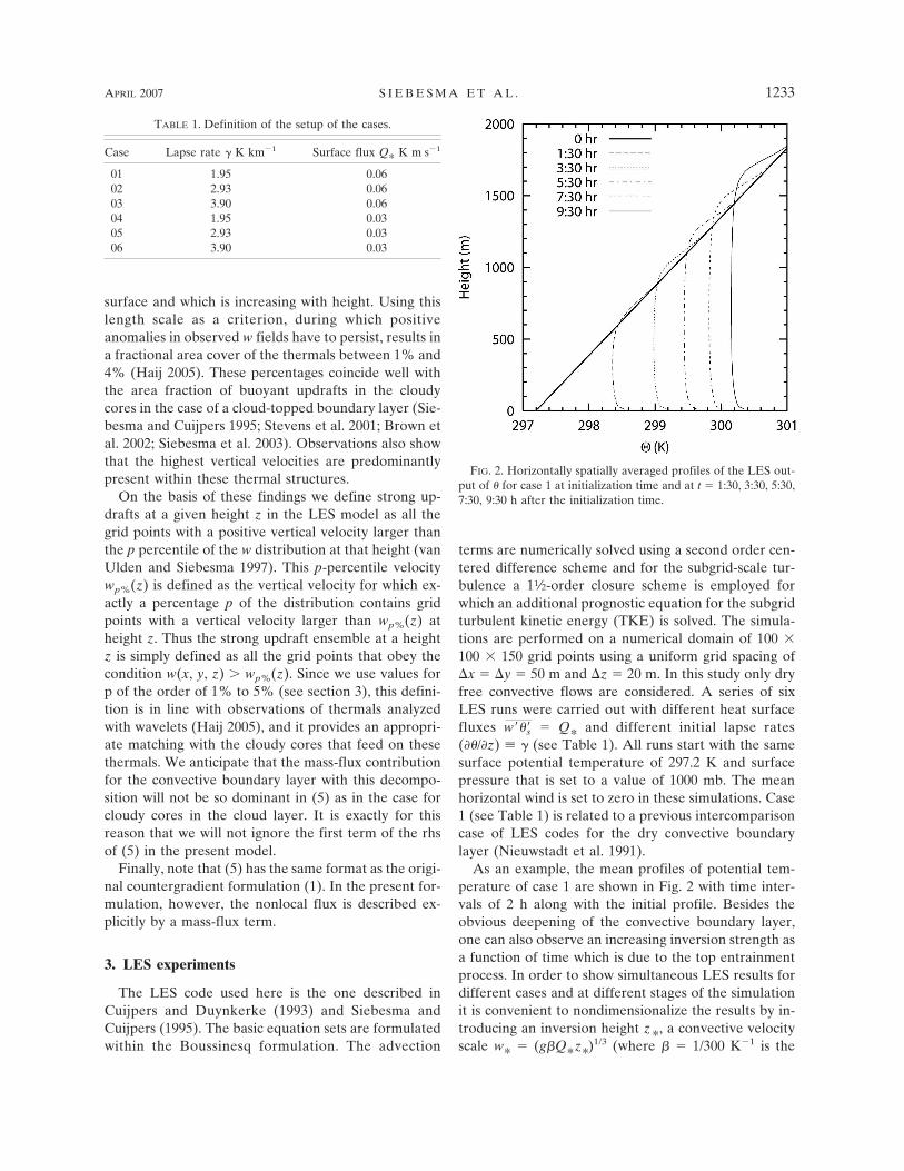
As an example, the mean profiles of potential tem-perature of case 1 are shown in Fig. 2 with time inter-vals of 2 h along with the initial profile. Besides theobvious deepening of the convective boundary layer,one can also observe an increasing inversion strength asa function of time which is due to the top entrainmentprocess. In order to show simultaneous LES results fordifferent cases and at different stages of the simulationit is convenient to nondimensionalize the results by in-troducing an inversion height z*, a convective velocityscale w* $ (g2Q*z*)1/3 (where 2 $ 1/300 K%1 is the

FIG. 2. Horizontally spatially averaged profiles of the LES out-put of # for case 1 at initialization time and at t $ 1:30, 3:30, 5:30,7:30, 9:30 h after the initialization time.

TABLE 1. Definition of the setup of the cases.

Case Lapse rate ) K km%1 Surface flux Q* K m s%1

01 1.95 0.0602 2.93 0.0603 3.90 0.0604 1.95 0.0305 2.93 0.0306 3.90 0.03


coefficient of thermal expansion), an eddy turnovertime t* + z*/w*, and a temperature scale #* + Q*/w*.As an operational definition of the inversion height z*we use the gradient method (Sullivan et al. 1998). Inthis method, for any location (x, y), the local inversionheight is determined as the height where # exhibits themaximum gradient. The (mean) inversion height z* isthen simply a spatial average over all the local inversionheights of the domain. This defines an inversion heightthat is slightly higher than the more conventional defi-nition of z* as the height where the buoyancy flux is aminimum (see Fig. 3a). The difference between thesedefinitions is of the order of 5% to 10% which impliesa difference of only 1% to 3 % for w* and #*. Oneadvantage of this definition is that it gives a smooth andcontinuous development of the boundary layer heightwith time (Sullivan et al. 1998).

Figure 3a shows the dimensionless heat fluxes w!#!/Q* as a function of the normalized height z/z* aver-aged over the ninth hour of the simulation for all cases.Note that the main difference for the dimensionlessfluxes between the different cases is in the entrainmentflux (i.e. the minimum value of the heat flux). Figure 3bzooms in further on this difference by showing the di-mensionless entrainment flux for all cases at all hours asa function of dimensionless time t̂ $ tN where N is theBrunt–Väisälä frequency. The dimensionless entrain-ment flux increases with time to values around 0.17 .0.2 in agreement with previous studies of the entrain-

ment zone (Fedorovich et al. 2004; Sullivan et al. 1998).The increase of the dimensionless entrainment flux isdirectly related with the sharpening of the inversionlayer with time, as measured by the Richardson numberRi $ 0#/#* where 0# is the temperature jump at theinversion. The lower values of the dimensionless en-trainment flux in the earlier stages of the runs are duea less pronounced inversion jump. For details on theentrainment processes in the inversion layer on the ba-sis of first- and second-order jump models we refer totwo excellent papers by Fedorovich et al. (2004) andSullivan et al. (1998).

In order to characterize the boundary layer growthfor all cases, we normalize z*(t) by the growth theboundary layer would have had in the absence of anytop entrainment. This so-called encroachment growthze(t) is easily calculated as (Stull 1988)

ze't( $ "2Q*$

t#1&2

. '6(

For all cases, z*/ze converges to values within the in-terval [1.2, 1.3] (see also Fig. 12). One of the majorevaluation tests will be whether the EDMF model andother related models are able to reproduce valueswithin this interval.

As discussed in the previous section we will use ppercentiles of the w field to define the strong updrafts.In order to display all mean and updraft profiles in one

FIG. 3. (left) Dimensionless turbulent heat flux profiles w!#!/Q*

as a function of the dimensionless height z/z* for the 10th hour forall six cases. (right) Hourly averaged dimensionless minimum heat flux values as a function of t̂.


plot we subtract the minimum value of the mean profile#min and rescale the result with #*. Figure 4 shows theresults for (# % #min)/#* and (#u % #min)/#* for p $ 1%,3%, 5% averaged over the sixth hour for all six cases. Anumber of observations can be made here that alsoapply to the other simulated hours. The average # pro-file is characterized by a super-adiabatic part up to 0.4z* and a slightly stable part from 0.5 z* upward. Theupdraft profile exhibits a positive temperature excess of1 . 4 times #* in most of the boundary layer but ischanging sign as the updraft penetrates into the inver-sion around 0.8 z*. Obviously, the excess temperatureis larger as we increase our threshold values wp%(z)through selecting smaller and more extreme updraftensembles. Finally note that the updraft potential tem-perature is decreasing with height, which is a sign oflateral mixing of the updraft ensemble with the envi-ronment.

Figure 4b displays the dimensionless updraft veloci-ties wu/w* along with the dimensionless standard devia-tion 3w/w* for p $ 1%, 3%, 5% again for all cases andaveraged over the sixth hour. Also shown is an empiri-cal expression for 3w based on a combination of atmo-spheric data, tank measurements, and LES data(Holtslag and Moeng 1991)

'w

w*! 1.3$" u*

w*#3

& 0.6z

z*%1&3"1 %

zz*#1&2

, '7(

where we use, in the absence of a mean horizontalwind, u* $ 0. The agreement in the boundary layer isgood while the nonzero contributions for 3w above theboundary layer is probably due to unphysical reflec-tions that create waves that are not adequately dampedby the sponge layer of the model. It can be observedthat the updraft vertical velocity profiles scale well with3w with a proportionality factor 4 $ (3w/wu)2 ! 0.15.This value is smaller than one would expect by assum-ing that the PDF of w is Gaussian. This is due to the factthe PDF of w is positively skewed (Wyngaard andMoeng 1992).

4. Eddy-diffusivity mass-flux parameterization forthe convective boundary layer

In this section, we will use the LES results of theprevious section to design a parameterization for tur-bulent heat transport in the convective boundary layer.Our starting point is (5). Therefore, our aim is to con-struct the simplest possible parameterization for the up-draft fields " ∈ {#, q*}; that is, to find an eddy-diffusivityK and a mass-flux M that are capable of realisticallyreproducing the time evolution of the boundary layerand the internal structure. We will also set up a param-eterization for the updraft velocity wu and use theheight where this velocity approaches zero as a measurefor the boundary layer height z*.

FIG. 4. (left) LES results of (# % #min)/#*

averaged over the sixth hour of the simulation along with updraft fields (#u % #min)/#* forp $ 1%, 3%, 5% for all cases. (right) LES results of the updraft vertical velocity for p $ 1%, 3%, 5% along with an LES profile of3w rescaled with w*. The line corresponds with the empirical expression (7).


a. The updraft model

The steady-state updraft budget equations for an ar-bitrary field " within the mass-flux approximation arewell known (Tiedtke et al. 1988; Siebesma and Holtslag1996) and can be written as

1M

#M#z

$ ( % ) '8(

#M%u

#z$ (M% % )M%u & auF%u

, '9(

where 5 and 6 denote the fractional entrainment anddetrainment rates, and F"u

contains all the externalsource and sink terms of the field " in the updraft areaau. For " $ #u we set F"u

$ 0; that is, we assume noeffects due to radiation and advection, so substitutionof (8) in (9) gives a simple entraining updraft equation

#"u

#z$ %('"u % "(. '10(

For the updraft velocity, the pressure and the buoyancyterm are the two main source terms (Schumann andMoeng 1991)

Fwu! % *%1 #p

#z& +g'",,u % ",(

+ P & B, '11(

where the term p represents the part of the pressurethat remains after subtracting the static pressure thatobeys hydrostatic equilibrium. Within the spirit of themass-flux approximation, we have neglected the pres-sure fluctuations within the updraft in (11). Substitutingthe forcing (11) in (9), using the definition of the mass-flux and rearranging terms gives the following steady-state budget equation for the vertical velocity

%12

#wu2

#z% (wwu

2 & B & P $ 0, '12(

where the first term represents a transport term (T),the second term the entrainment term (E), and the lasttwo terms represent the buoyancy and the pressure gra-dient term.

Note that we attached a w subscript to the fractionalentrainment rate in (12) to indicate that the fractionalentrainment rate of w can, in principle, be differentfrom the entrainment rate of # (de Roode and Brether-ton 2003). The pressure term can conveniently be ex-pressed in terms of the vertical velocity variance (Schu-mann and Moeng 1991)

P $ %1*

#p#z

$#w2

#z!

#-wu2

#z, '13(

where, in the last step, we have made use of the factthat w2

u scales well with the vertical velocity variancewith a proportionality factor 4 ! 0.15 as discussed in theprevious section. Finally, we assume that the fractionalentrainment rate for the vertical velocity 5w is propor-tional to the fractional entrainment rate for #; that is,

(w $ b(. '14(

Substituting (14) and (13) into the vertical updraft ve-locity equation (12) gives

12 '1 % 2-(

#wu2

#z$ %b(wu

2 & B. '15(

Note that this vertical velocity equation has the sameform as the one proposed by Simpson and Wiggert(1969) for cloudy plumes and which is widely used inmoist convection parameterizations. The physical inter-pretation of the terms, however, is quite different.

The fractional entrainment rate 5 is diagnosed usingLES results for # and #u in (10). For the sixth hour weshow in Fig. 5 the dimensionless fractional entrainmentrate 5z* for p $ 1%, 3%, 5% for all cases. Althoughsome systematic spread can be observed for these threedefinitions, the points collapse reasonably well on asingle parabolic curve that can be well fitted with

( ! c("1z

&1

z* % z# '16(

FIG. 5. LES results for the nondimensionalized reciprocal frac-tional entrainment rates 1/(5z*) diagnosed using (10) for p $ 1%,3%, 5% for all six cases averaged over the sixth hour. The full linerepresents the parameterized form (16).


with c5 ! 0.4. This parabolic shape, already proposed invan Ulden and Siebesma (1997), strongly suggests thatthe entrainment length scale 5%1(z) is determined bythe dominant eddy size at height z (see also Fig. 1).Such an identification also explains the strong resem-blance between 5%1 and the length scale used in TKEschemes (Cuxart et al. 2000; Bougeault and Lacarrère1989; Teixeira et al. 2004). The use of (10) to diagnose5 becomes ill defined when the excess has a zero cross-ing. This explains the scatter of the diagnosed value of5 in Fig. 5 around the inversion.

The 5 . z%1 behavior near the surface has been re-ported recently also, based on LES results, for a simpleupdraft–downdraft decomposition (de Roode et al.2000). The z%1 scaling has the advantage that the pre-cise choice of the initialization height z1 becomes irrel-evant in the limit of a neutral boundary layer. Moreprecisely, if # has a logarithmic profile, it is easy toshow, using (10) that for 5 . z%1 the excess #u % #becomes height independent (see appendix A). For thepresent cases, which are in the free convective limit, # isdescribed by a power law in the surface layer. In thatcase, there is still a small dependency of the tempera-ture excess, but still much smaller than in the case of anonentraining adiabatic ascending plume.

Next we will evaluate the vertical velocity budgetequation (12) with the LES results in its parameterized

form. For the pressure term we use the right-hand sideof (13), for the mixing term we use (14) along with thefit (16) for 5. We finally close the budget equation (12)of w by solving for b at each height level that is theremaining undetermined parameter [see (14)]. Thebudget terms are nondimensionalized by w2

*/z* andshown in the left panel of Fig 6. This allows averages tobe shown over the sixth hour of the budget equation forall six cases. It can be observed that the most importantsource term for the updraft vertical velocity is the buoy-ancy term. The entrainment term is a remarkable con-stant sink term while the pressure term is a source termin the lower half of the boundary layer and a sink termin the upper half. Overall the sum of the three budgetterms (B, P, E) generate a net source term in the lowerpart of the boundary layer and a net sink term in theupper part. This is compensated by the transport termT, reflecting the fact that kinetic energy is transportedfrom the lower half to the upper half of the boundarylayer by the nonlocal strong thermals.

The diagnosed profile of the scaling factor b is dis-played in Fig. 6b. The fact that the diagnosed value ofb is rather independent of height and time is a justifi-cation for the assumption that 5w can be scaled with 5 bya constant factor. The result suggests b ! 0.5, a valuethat we will adopt in the parameterization and the one-column simulations in the next section.

FIG. 6. (a) Nondimensionalized budget terms of the updraft velocity equation (12) as a function of the relative height for all casesaveraged over the sixth hour, where T is the transport term, E is the entrainment term, B is the buoyancy term, and P is the pressuregradient term. (b) The corresponding diagnosed entrainment scaling parameter b [see (14)].


Finally, we initialize the updraft model by taking themean value at the lowest model level z1 and adding anexcess that scales with the surface flux (Troen andMahrt 1986)

"u'z1( $ "'z1( & .Q*

'w'z1(, '17(

where w!#!s is the surface flux. For the standard devia-tion 3w we use the empirical expression (7). The valueof the prefactor 7 again is based on LES results thatsuggest 7 ! 1. Note that this value is much smaller thanthe value of 7 ! 8 originally proposed in (Troen andMahrt 1986).

This completes the updraft model that calculates,given the surface fluxes and the mean profiles, the up-draft fields of #u, qu, and wu, and the inversion heightz*, the latter being the height where wu vanishes.

b. Eddy diffusivity and mass flux parameterization

To complete the EDMF approach (5) we need tospecify the eddy diffusivity K and the mass flux M. Asimple and robust method for the convective boundarylayer is to use a profile method (Troen and Mahrt 1986)and we will do so accordingly. A so-called K profileshould at least

• obey surface layer similarity near z $ 0,• vanish near the inversion,• exhibit a peak value Kmax/(w*z*) ! 0.1.

Holtslag (1998) proposed a K-profile Kh for heat andmoisture that obeys these constraints that we will adopthere. In a nondimensionalized form it reads

K̂h +Kh

z*w*$ k

u*w*

%h0%1 z

z*"1 %

zz*#2

, '18(

with k the von Kármán’s constant and "h0 an effectivestability function given by

%h0 $ "1 % 39zL#%1&3

, '19(

where L is the Obukhov length. Eliminating theObukhov length in terms of z* and w* finally gives

K̂h $ k$" u*w*#3

& 39kz

z*%1&3 z

z*"1 %

zz*#2

.

'20(

Note that (20) is about proportional to the product of3w as given by (7) and a length scale similar to the onegiven by (16). This observation illustrates the analogybetween the present K-profile method and methods in

which the eddy-diffusivity is estimated as a product of alength scale and a velocity scale. Since surface layersimilarity determines the surface fluxes and the updraftmodel determines the inversion height z*, (20) com-pletely determines the eddy diffusivity profile.

The mass-flux M ! auwu is directly proportional towu since au is constant by definition. This allows themass flux to scale with the standard deviation 3w (seeFig. 4b)

M $ cm'w , '21(

with cm ! 0.3 and where we use the parameterized form(7) for 3w. Alternatively one can also directly use thedefinition of the mass flux M ! auwu and use the up-draft velocity equation (15) (Soares et al. 2004).

c. Implementation of the scheme

An often-undervalued aspect of any parameteriza-tion is its numerical implementation. The numericalchallenge of the present scheme is how to discretize thetime evolution equation (2) due to turbulent mixing asestimated by the present EDMF approach (5) for " ∈{#, q*}

"#%

#t #mix$ %

#w!%!

#z

$ %#

#z $%K#%

#z& M'%u % %(%. '22(

In order to solve this advection–diffusion equation in aconsistent manner, a full advection–diffusion solver isused. The diffusion and the mass-flux coefficients canbe quite large when compared with the time step andvertical grid space typically used in climate and NWPmodels. In fact, these coefficients often exceed the nu-merical stability limits for both the diffusion and advec-tion explicit schemes. Because of this, the typical tur-bulent diffusion equation in climate and NWP models isgenerally solved in an implicit manner (Girard andDelage 1990; Beljaars 1991).

The advective mass-flux transport, however, is usu-ally treated in an explicit manner, although it has beenshown that the mass-flux term violates the stability cri-terion on a regular basis (Jakob and Siebesma 2003). Inorder to address these stability problems, the mass-fluxand diffusion terms in the present scheme are solvedsimultaneously in an implicit manner according to analgorithm already tested in the European Centre forMedium-Range Weather Forecasts (ECMWF) model(Teixeira and Siebesma 2000). For details on the nu-merical discretization of (22), we refer to appendix B.


5. Single-column model results

a. Reference case

We will proceed by using case 1 as described in sec-tion 3 to evaluate the EDMF parameterization. Al-though this case has been used to design the param-eterization, it is still a useful test since it answers thequestion to which extent the mean turbulent transportin three dimensions can be faithfully represented in onedimension. To this purpose a single-column model(SCM) with the above-described EDMF scheme hasbeen developed. For the time stepping the implicitscheme described in appendix B is used. The values ofthe constants in the reference case are based on theLES results discussed in the previous section and whichare summarized in Table 2.

In order to exclude possible errors due to a too-coarse resolution we use in the reference run the samehigh vertical resolution of 20 m as in the LES model.Additionally we also repeat the same experiment with acoarser resolution to assess to what extend the param-eterization is sensitive to the used vertical resolution.This low-resolution run uses the same resolution as inthe 60-level operational ECMWF model (Teixeira1999). For the present simulations, only the lowest thir-teen levels are active, which are at about 10, 35, 75, 125,200, 295, 410, 560, 730, 930, 1165, 1430, 1725, and 2050m.

The boundary layer growth is critically dependent onthe model formulation of the inversion height z* be-cause of the use of a K-profile method. Therefore careis needed to determine z* on a discretized grid in orderto avoid possible resolution dependencies. Therefore,two modifications to the model formulation are added.First the inversion height z*, defined as the height atwhich the vertical velocity vanishes, is determined byfinding the zero-crossing of the updraft velocity by in-terpolation between the highest level with a positive wu

and the subsequent level that has a negative verticalvelocity. This allows a smooth growth of the boundarylayer height. Second, since near the inversion the en-trainment term becomes increasingly important, we

propose a modified formulation of the lateral entrain-ment to reduce the resolution sensitivity

( ! c($ 1z & /z

&1

'z* % z( & /z%, '23(

where 0z represents the vertical grid size where 5 isevaluated. Note that in the limit of high-resolution0z → 0 the original formulation (16) is recovered. Theaddition of the factor 0z assures the entrainment nearthe inversion can never exceed c5/0z, which is a rea-sonable upper limit for the grid-averaged lateral en-trainment near the inversion.

Since we do not want that any spinup effects of theLES model runs influence the evaluation, we initializethe SCM with mean profiles of the LES model after 0.5h of simulation (see Fig. 7a). Figure 7a shows the SCMresults after 5 and 10 h of simulation along with thecorresponding LES results. It can be observed that thetemperature evolution of the boundary layer is wellreproduced by the SCM, also in the low-resolutionmode. This suggests that the boundary layer growthand the top-entrainment process are well captured bythe SCM. This hint is confirmed in Fig. 7b where theboundary layer (BL) height evolution of the SCM isshown and compared with the LES results. The wiggledstructure of the BL height growth for the low resolutionis the only remnant of the coarse resolution.

Figure 7c focuses more on the internal dynamics ofthe model. Figure 7c evaluates the nondimensionalizedupdraft velocity after 10 h of simulation. This resultindicates that the updraft model is not only producingthe correct boundary layer growth but also the properupdraft characteristics. Finally, in Fig. 7d, the nondi-mensionalized resulting heat flux after 10 h of simula-tion is displayed along with the flux from the LESmodel. Moreover, the breakdown of the turbulent fluxof the EDMF scheme into the contribution of the dif-fusion term and the nonlocal mass flux is shown in thesame figure. A couple of remarks should be made here.First it should be observed that both terms contributeto the negative entrainment flux in the inversion: thediffusion term because it is downgradient and the mass-flux contribution because the updraft temperature islower than the mean temperature in the inversion. Sec-ond, the mass-flux term provides, except in the surfacelayer, the dominant contribution to the turbulent flux.In fact it turns out, as we will see in the next subsection,that the precise magnitude of the eddy diffusivity is notthat relevant.

b. Model sensitivity

It is good practice to provide insight on the sensitivityof the parameterization scheme to the used parameters.

TABLE 2. The values of the constants based on the LES resultsthat are used in the reference SCM run. The third column showsthe variation of these parameters to assess the sensitivity of thescheme to these constants in section 5b.

Parameter Reference value Sensitivity variation

c5 0.4 0.38 0 c5 0 0.42cm 0.3 0.24 0 cm 0 0.36b 0.5 0.4 0 b 0 0.64 0.15 0.12 0 4 0 0.187 1.0 0.8 0 7 0 1.2


As an integral measure for the sensitivity, the boundarylayer height after 10 h of simulation is evaluated. Eachof the parameters displayed in Table 2 is increased anddecreased by 20% and the effect of this change on theboundary layer height is shown in Fig. 8.

The largest sensitivities are due to the parameters c5

and b, which determine the intensity of the lateral en-trainment. The sensitivity cm that determines thestrength of the mass-flux contribution is rather small.Also, the sensitivity to the initialization of the tempera-

FIG. 7. Single-column model results with a high (dots) and a low (dashes) vertical resolution of the EDMF scheme evaluated withLES results (full lines); (a) initial vertical profile and profiles after 5 and 10 h of simulation, (b) time evolution of the boundary layerheight, (c) nondimensionalized updraft velocity of the thermal after 10 h of simulation, and (d) the total nondimensionalized turbulentflux, produced by the LES model (thick full line) and the SCM (thin full line) after 10 h of simulation. Also displayed is the breakdownof the turbulent flux of the EDMF scheme into the diffusion contribution (dashes) and a contribution due to the mass-flux term (dots).


ture excess as expressed by the factor 7 is small. This isbecause the sensitivity is strongly damped by the lateralentrainment of the updraft. In short, the most sensitiveparameters are those that directly influence the deter-mination of the boundary layer height, since z* deter-mines the growth rate of the boundary layer height andhence the top-entrainment flux.

There is also a remarkable insensitivity to the eddydiffusivity K that was already briefly mentioned in theprevious subsection. In order to quantify this aspect,the intensity of the K profile (20) is also increased anddecreased by 20% without any effect on the model out-put. In fact, we are able to reduce the effect of the Kprofile by 80% without any significant effect on themodel. Similar to Fig. 7d we show in Fig. 9 the breakupof the total heat flux into the diffusive contribution andthe mass-flux contribution after 10 h of simulation forthis reduced diffusion case. It can be observed that al-most the entire heat flux is faithfully reproduced by themass-flux contribution only, except near the surfacewhere the diffusion is still the dominant term. Onemight argue that this observation would promote a pa-rameterization in terms of mass flux only. However, westrongly think that the inclusion of a diffusion term iscrucial for a number of reasons. First, in the presentconvective case it is true that the precise value of thediffusion is not that important, but if we lower the am-plitude of the K profile even further by 90% the modelbecomes unstable near the surface and strong wiggles inthe separate flux contributions can be seen. In thepresent convective case, the diffusion acts mainly as astabilizing smoothing operator. Second, the role of thediffusion will become more physically relevant in thecase of a transition to neutral or stable boundary layer.In that case, the nonlocal mass flux contribution willvanish and the diffusion has to be the main mixingmechanism. With only a mass-flux parameterization, a

smooth transition to and a proper parameterization ofthe neutral and stable boundary layer will become un-necessarily painful.

c. Other approaches

In this section, we want to confront the EDMF ap-proach with two other more traditional methods. Thefirst one is the usual ED approach without any extranonlocal modifications. The second approach is to use acountergradient (EDCG) term to take into accountnonlocal transport. In formula this second approach isgiven by (1) where we choose for the nonlocal term )the formulation suggested by Cuijpers and Holtslag(1998)

$ $ aw*

'w2 z*

w!"!*, '24(

with a ! 2. The three approaches are summarized inTable 3. We emphasize that, in order to make the com-parison as clean as possible, in all three cases the sameK-profile method with the same vertical velocity equa-tion (15) is used to determine the BL height z*. Thisway we can assess in a transparent way the impacts ofthe classic countergradient approach and the mass-fluxcontribution to the bare eddy diffusivity approach.

FIG. 8. Effect of the variation of the used constants in theEDMF scheme as given in Table 2 on the boundary layer heightafter 10 h of simulation. Note that the parameters with the strong-est sensitivity are those that directly influence the determinationof the BL height.

FIG. 9. The same as in Fig. 7d but now with a run in which theK coefficient is reduced by 80% with respect to the reference run.Note that the turbulent flux is almost completely determined bythe mass-flux term and that even after 10 h of simulation the SCMflux profile is similar to the flux profile produced by the LESmodel.


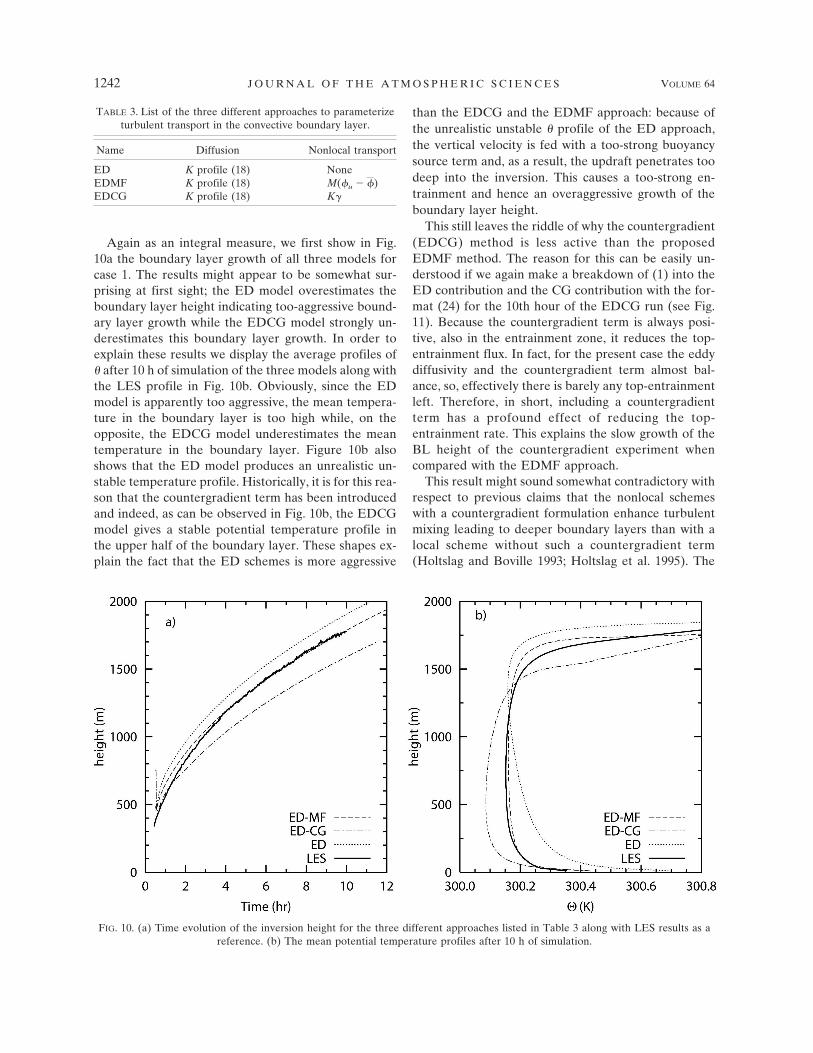
Again as an integral measure, we first show in Fig.10a the boundary layer growth of all three models forcase 1. The results might appear to be somewhat sur-prising at first sight; the ED model overestimates theboundary layer height indicating too-aggressive bound-ary layer growth while the EDCG model strongly un-derestimates this boundary layer growth. In order toexplain these results we display the average profiles of# after 10 h of simulation of the three models along withthe LES profile in Fig. 10b. Obviously, since the EDmodel is apparently too aggressive, the mean tempera-ture in the boundary layer is too high while, on theopposite, the EDCG model underestimates the meantemperature in the boundary layer. Figure 10b alsoshows that the ED model produces an unrealistic un-stable temperature profile. Historically, it is for this rea-son that the countergradient term has been introducedand indeed, as can be observed in Fig. 10b, the EDCGmodel gives a stable potential temperature profile inthe upper half of the boundary layer. These shapes ex-plain the fact that the ED schemes is more aggressive

than the EDCG and the EDMF approach: because ofthe unrealistic unstable # profile of the ED approach,the vertical velocity is fed with a too-strong buoyancysource term and, as a result, the updraft penetrates toodeep into the inversion. This causes a too-strong en-trainment and hence an overaggressive growth of theboundary layer height.

This still leaves the riddle of why the countergradient(EDCG) method is less active than the proposedEDMF method. The reason for this can be easily un-derstood if we again make a breakdown of (1) into theED contribution and the CG contribution with the for-mat (24) for the 10th hour of the EDCG run (see Fig.11). Because the countergradient term is always posi-tive, also in the entrainment zone, it reduces the top-entrainment flux. In fact, for the present case the eddydiffusivity and the countergradient term almost bal-ance, so, effectively there is barely any top-entrainmentleft. Therefore, in short, including a countergradientterm has a profound effect of reducing the top-entrainment rate. This explains the slow growth of theBL height of the countergradient experiment whencompared with the EDMF approach.

This result might sound somewhat contradictory withrespect to previous claims that the nonlocal schemeswith a countergradient formulation enhance turbulentmixing leading to deeper boundary layers than with alocal scheme without such a countergradient term(Holtslag and Boville 1993; Holtslag et al. 1995). The

FIG. 10. (a) Time evolution of the inversion height for the three different approaches listed in Table 3 along with LES results as areference. (b) The mean potential temperature profiles after 10 h of simulation.

TABLE 3. List of the three different approaches to parameterizeturbulent transport in the convective boundary layer.

Name Diffusion Nonlocal transport

ED K profile (18) NoneEDMF K profile (18) M("u % ")EDCG K profile (18) K)


reason for this is that in these studies, the eddy-diffusivity formulations used for the local and nonlocalschemes are not the same. The reason that the nonlocalscheme appears to be more active despite the counter-gradient term is due to the use of an aggressive K-profile method with a parcel method to estimate the BLheight. The present results in this study are qualita-tively in agreement with the findings of Stevens (2000)who found, using 1-yr integrations of the standardCommunity Climate Model (CCM) version 3.2 withfixed SSTs (Kiehl et al. 1996), that switching off thecountergradient term leads to an increase of the glo-bally averaged BL height.

d. Evaluation of the model with the other LEScases

So far we have limited our evaluation of the EDMFmodel and other approaches to case 1. We conclude ourstudy by evaluating the boundary layer growth for allsix cases for the reference EDMF model, the EDCGmodel, and the ED model, and compare these resultswith the LES data. As already mentioned in section 3,a critical test for these models is whether they can re-produce the dimensionless boundary layer height z*/ze

for the limit t̂ → 8. As none of these schemes havethe level of sophistication to incorporate the depen-dency of the entrainment flux on the Richardson num-ber (see Fig. 3b), it is not realistic to expect that these1d-models can reproduce the variation of z*/ze fromcase to case.

The test will therefore be whether the abovemen-tioned models are capable of reproducing values ofz*/ze that fall within the range of z*/ze produced bylarge-eddy simulations. The LES results are shown inFig. 12. The thick line is the time evolution of z*/ze forthe ensemble mean LES results, while the standard de-viation of z*/ze based on the six cases is shown as agray band around the mean. The results for all sixcases for the EDMF, EDCG, and the ED model areplotted in this Fig. 12 as well. This shows that the resultsfound for case 1 are quite generic: the EDMF modelgenerates boundary layer growth for all cases that fallwithin the range [1.2, 1.3] and compare reasonably wellwith the LES results. The EDCG model underesti-mates the boundary layer growth in all cases while theED model overestimates the boundary layer growth inall cases.

6. Conclusions and perspectives

Convective boundary layers are ubiquitous in the at-mosphere and they have a fundamental impact on thephysics and dynamics of the climate system. However,due to coarse horizontal resolution, the turbulent and

FIG. 11. Total heat flux of the LES model after 10 h of simula-tion along with the heat flux of the SCM model with the coun-tergradient approach. Also shown is the breakup of the heat fluxin the SCM model into a contribution due to the eddy diffusivityand a contribution due to the countergradient term ). Note thatthe countergradient contribution is working against the entrain-ment flux. As a result, there is an almost zero entrainment fluxleft.

FIG. 12. Dimensionless boundary layer–growth evaluation ofthe EDMF model (thin full lines), the EDCG model (dashed),and the ED model (dotted) for all six cases defined in Table 1along with the LES results. These are shown as an ensemble mean(thick line) and a band that indicates the standard deviation of theensemble.


convective flow within the boundary layer cannot beexplicitly resolved by current weather (global or meso-scale) and climate prediction models. Parameteriza-tions of these subgrid fluxes are then necessary in orderto achieve some level of realism. In spite of its apparentsimplicity, due to the lack of condensation effects, dryconvective boundary layers are still a major challengein weather and climate modeling, in particular the rep-resentation of the boundary layer top-entrainment andthe countergradient fluxes.

In this paper we propose a unified way of represent-ing the subgrid vertical flux in dry convective boundarylayers, by combining the eddy-diffusivity (ED) ap-proach (typically used for the parameterization of dryand stratus/stratocumulus boundary layers in weatherand climate prediction models) with the mass-flux (MF)approach (typically used for the parameterization ofshallow and deep moist convection).

The EDMF approach is based on the idea that theMF closure is able to represent what we refer to asnonlocal transport due to the strong thermals, while theED closure is able to represent the more local turbulenttransport. In section 2, it is shown that the EDMF clo-sure follows naturally from a decomposition of the sub-grid vertical transport into 1) the strong organized up-drafts, and 2) the remaining environment.

In section 3, numerical simulations of the dry con-vective boundary layer were carried out with a large-eddy simulation (LES) model. These simulations wereused to establish the EDMF concept in a more solidbase and to obtain estimates for the parametersneeded, such as the updraft model, ED and MF coef-ficients.

LES results were also used to evaluate the newEDMF parameterization. When compared to LES, thenew closure represents well the evolution of the mainproperties of the dry convective boundary layer. Theoverall growth of the boundary layer is reproduced inan accurate way, even when a relatively poor verticalresolution is used. This result means that the EDMFrepresentation of the top-entrainment must be particu-larly realistic. The well-mixed nature of the potentialtemperature profile is achieved in a, probably, unprec-edented manner. The linear nature of the buoyancyflux profile, quasi-parabolic nature of the updraft ver-tical velocity, and updraft temperature are also shownto be realistic when compared to LES results.

Some of the current alternatives, in particular theexplicit parameterization of the countergradient fluxes,are analyzed in some detail and compared to theEDMF approach. It is shown that the more traditionalcountergradient closures indeed reproduce a correct in-ternal structure of the boundary layer, but at the ex-

pense of strongly underestimating the ventilating topentrainment. The reason for this last point has beenshown to be associated with the negative impact thatthe countergradient term has at the entrainment level.

Historically, to our knowledge, Chatfield and Brost(1987) were the first to apply a mass-flux approach toan updraft–downdraft decomposition and combine thiswith an eddy-diffusivity approach for the remainingsubplumes to study scalar transport in the dry convec-tive boundary layer. The importance of these sub-plumes for the total turbulent transport was studied indetail for reactive scalars in the convective boundarylayer by Petersen et al. (1999). That concept has beenfurther extended in a higher-order closure frameworkby Lappen and Randall (2001a,b) and has been appliedto both dry and moist convection by these authors.

The present EDMF scheme is based on the ideasfrom Siebesma and Teixeira (2000) and differs from theprevious studies most notably in the definition of theupdrafts: since the primary motivation for this studywas to establish a continuous formulation between drythermals in the convective boundary layer and the en-training plumes within the cloud layer, a straightfor-ward updraft–downdraft decomposition is not appro-priate. It is for this reason that the strong updraft defi-nition presented in section 3 has been used: LES resultsshow that the strongest updrafts at the top of the sub-cloud layer actually do form the cloudy cores at cloudbase. Therefore, the main advantage of this avenue isthat it naturally opens the way for a scheme of thecloud-topped boundary layer by allowing the moisturein the strong updraft to condense. No switching of amoist convection scheme is then necessary anymore. Insuch a case, the updraft model is always active anddecides independently whether these updrafts becomecloud-core updrafts or not.

The present version of the EDMF scheme for the dryconvective boundary layer is part of the ECMWFmodel since cycle 29.3 that became operational in April2005. The EDMF framework also has been imple-mented successfully in the nonhydrostatic mesoscale at-mospheric model of the French research community(Meso-NH; Soares et al. 2004). One main differencewith the present formulation is that the eddy-diffusivityin Soares et al. (2004) is calculated using a prognosticturbulent kinetic energy (TKE) equation (Cuxart et al.2000). Let us emphasize here that the specific choice ofhow to calculate the eddy diffusivity (TKE or K profile)is important, but not essential for the principle of theEDMF framework.

We would like to conclude with some thoughts onhow to extend this framework to the cloudy boundarylayer. In Soares et al. (2004), the extension of the


EDMF approach to moist convection has been studied.The updraft equations have been extended by allowingfor condensation. Above cloud base, a constant frac-tional entrainment rate of 5 $ 2 10%3 m%1 is used andthe mass flux is determined below cloud base by M $auwu where the updraft velocity wu follows from theupdraft equation (15), while above cloud base the massflux is simply diagnosed from the cloud-core continuityequation (8). This form of the EDMF scheme has beenimplemented in the Meso-NH model and evaluatedwith observations from the Atmospheric RadiationMeasurement (ARM) Southern Great Plains (SGP)site on 21 June 1997 during which a typical diurnal cycleof cumulus convection was observed (Brown et al. 2002;Lenderink et al. 2004).

At ECMWF, the EDMF framework has been ex-tended by enhancing the dry K profile (20) to moistconditions in order to allow for diffusive mixing in thestratocumulus-topped boundary layer as proposed byvan Meijgaard and van Ulden (1998). The eddy diffu-sivity is then based on both surface and cloud-top forc-ing. This parameterization is operational since April2005 and drastically improves the representation of ma-rine stratocumulus with additional benefits to continen-tal winter stratus (Koehler 2005). At the moment, theEDMF framework is being extended to shallow con-vection as well in the ECMWF model using multiplemass-flux terms (Cheinet 2003). The EDMF approachhas also been recently successfully applied to pollutanttransport in the cumulus-topped boundary layer (An-gevine 2005).

A number of open questions still remain that providean active source of research at this moment. First, thereis the issue of what to use for the fractional entrainmentformulation. Soares et al. (2004) essentially use a com-bination of the present formulation (16) combined witha typical constant value above cloud base that is diag-nosed from LES studies for shallow cumulus convec-tion (Brown et al. 2002; Siebesma et al. 2003). An in-teresting alternative has been proposed by Cheinet(2003) and is a combination of the present formulation(16) and a formulation that has been proposed in Neg-gers et al. (2002)

( + max" 11wu

,c(

z #, '25(

where 9 represents the eddy turnover time. In the lowerpart of the boundary layer the c5/z term dominateswhile in the upper part of the boundary layer and in thecloud layer the entrainment rate is determined by1/(9wu). Indeed the fractional entrainment rate is aboutinversely proportional to the updraft vertical velocity.The simple rational behind this behavior is that slow

updrafts have simply more time to mix with environ-mental air than fast updrafts. This formulation has theadvantage that it works in the cloud layer as well as inthe subcloud layer and, moreover, it does not requirethe inversion height z* as an input variable. Second,there is the issue of the updraft velocity equation. Theformulation (15) is identical to formulations used inmoist convection schemes (Gregory 2001) but with dif-ferent coefficients. A similar diagnosis for the updraftvelocity equation in the cloudy core should shed somelight on this issue. Third, there is the issue of the massflux. For the clear boundary layer, one can use the ver-tical velocity variance to scale the mass-flux (21) butthis scaling does not hold anymore in the cloud layer.Using the updraft velocity wu instead (Soares et al.2004) is an interesting alternative that automaticallyprovides a closure for the mass flux at cloud base that isclosely related to the mass-flux closures proposed byGrant (2001) and Neggers et al. (2004).

Let us finally note that the present proposed formu-lation can be extended to multiple entraining plumes.Recent studies have shown that multiple entrainingplumes can give an accurate description of the turbu-lent transport and the variability in both the clear(Cheinet 2003) and the cloud-topped boundary layer(Cheinet 2004; Neggers et al. 2002). The present study,however, shows that, as far turbulent transport in theconvective dry boundary layer is concerned, one up-draft equation is sufficient.

Acknowledgments. This research was initiated whilethe first author, A. Pier Siebesma, was invited to workas a consultant at the ECMWF. It is therefore a plea-sure to thank Anton Beljaars and Martin Miller fortheir keen interest in this topic. We also want to thankAad van Ulden for many useful suggestions during ear-lier stages of the design of this scheme. Bjorn Stevensand two anonymous reviewers are acknowledged forthe many valuable suggestions on a first draft of thepaper and Stephan de Roode and Geert Lenderink fora critical reading of the manuscript. The work done byPedro M. M. Soares was supported by Fundacão para aCiência e Tecnologia (FCT) under Project BOSS/58932/2004, cofinanced by the European Union underProgram FEDER, and by the EU Grant EVK2 CT19990005 (EUROCS).

APPENDIX A

Analytical Results for the Updraft Fields in theSurface Layer

LES results suggest a power-law behavior of 5 nearthe surface


( !c(

z. 'A1(

If we use substitute this in the updraft equation for afield "

#%u

#z$ %('%u % %(, 'A2(

we obtain a general solution of the form

%u'z( $ Az%c( & c(z%c(& %'z(zc( % 1 dz. 'A3(

Assuming a logarithmic profile for " in the surfacelayer

%'z( $ %'z0( % c% lnzz0

, 'A4(

and an excess of 0"u(z0) of the updraft field at an ar-bitrary height z0 in the surface layer; that is, "u(z0) $"(z0) & 0"u(z0), we find

%u'z( $ %'z0( & /%u'z0( % c% lnzz0

, 'A5(

which directly proves that that the excess of the updraftfield; that is, "u(z) % "(z), remains constant as a func-tion of height. This implies that the updraft field "u(z)does not depend on the position z0 in the surface layerwhere it is initialized.

APPENDIX B

Discretization of the EDMF Equation

Equation (22) is solved with the following discretiza-tion in time

%t&/t % %t

/t$ %

#

#z $%Kt #%t&/t

#z& Mt'%u

t % %t&/t(%,

'B1(

where we skipped the average bar in order to simplifynotation. The generic variable " on the rhs is takenimplicitly, but the ED and MF coefficients and the up-draft fields are taken explicitly. This occurs due to thenonlinear way of calculating these coefficients, whichwould lead to nonlinear implicit solvers if the coeffi-cients were considered in an implicit manner.

For the space discretization, centered differences inspace are used for the diffusion term and an upwindscheme is used for the mass-flux term. The fully dis-cretized version of the equation is (assuming K and Mare constant in space for notation simplicity)

%.%z%/zt&/t & '1 & 2. & +(%z

t&/t

% '. & +(.%z&/zt&/t $ %z

t & Czt , 'B2(

where 7 $ Kt0t/0z2 and 2 $ Mt0t/0z and the term Ccontains the source terms and the term that involves theupdraft values that are taken explicit in time.

Although the present model has not shown any sta-bility problems with the resolutions and time steps thatwere used, and since the different prognostic equationscan be highly nonlinear, the present quasi-implicitscheme proposed may not be sufficiently stable for allcases. This is actually a common and open problem inweather and climate prediction models and in the fu-ture more stable solutions will be necessary.

REFERENCES

Angevine, W. M., 2005: An integrated turbulence scheme forboundary layers with shallow cumulus applied to pollutanttransport. J. Appl. Meteor., 44, 1436–1452.

Arakawa, A., 1969: Parameterization of cumulus convection.Proc. IV WMO/IUGG Symp. on Numerical Prediction, Vol.8, Tokyo, Japan, Japan Meteorological Agency, 1–6.

Beljaars, A. C. M., 1991: Numerical schemes for parameteriza-tions. Proc. Seminar on Numerical Methods in AtmosphericModels, Reading, United Kingdom, ECMWF, 1–42.

Betts, A. K., 1973: Non-precipitating cumulus convection and itsparameterization. Quart. J. Roy. Meteor. Soc., 99, 178–196.

Bougeault, P., and P. Lacarrère, 1989: Parameterization of orog-raphy-induced turbulence in a mesobeta-scale model. Mon.Wea. Rev., 117, 1872–1890.

Brown, A. R., and Coauthors, 2002: Large-eddy simulation of thediurnal cycle of shallow cumulus convection over land. Quart.J. Roy. Meteor. Soc., 128, 1075–1094.

Chatfield, R. B., and R. A. Brost, 1987: A two-stream model ofthe vertical transport of trace species in the convectiveboundary layer. J. Geophys. Res., 92, 13 263–13 276.

Cheinet, S., 2003: A multiple mass-flux parameterization for thesurface-generated convection. Part I: Dry plumes. J. Atmos.Sci., 60, 2313–2327.

——, 2004: A multiple mass flux parameterization for the surface-generated convection. Part II: Cloudy cores. J. Atmos. Sci.,61, 1093–1113.

Cuijpers, J. W. M., and P. J. Duynkerke, 1993: Large-eddy simu-lation of trade-wind cumulus clouds. J. Atmos. Sci., 50, 3894–3908.

——, and A. A. M. Holtslag, 1998: Impact of skewness and non-local effects on scalar and buoyancy fluxes in convectiveboundary layers. J. Atmos. Sci., 55, 151–162.

Cuxart, J., P. Bougeault, and J.-L. Redelsperger, 2000: A turbu-lence scheme allowing for mesoscale and large-eddy simula-tions. Quart. J. Roy. Meteor. Soc., 126, 1–30.

Deardorff, J. W., 1966: The counter-gradient heat flux in thelower atmosphere and in the laboratory. J. Atmos. Sci., 23,503–506.

——, 1972: Theoretical expression for the counter-gradient verti-cal heat flux. J. Geophys. Res., 77, 5900–5904.

de Haij, M. J., 2005: Evaluation of a new trigger function of con-vection. KNMI Tech. Rep. TR-276, 117 pp.


de Roode, S. R., and C. S. Bretherton, 2003: Mass-flux budgets ofshallow cumulus clouds. J. Atmos. Sci., 60, 137–151.

——, P. G. Duynkerke, and A. P. Siebesma, 2000: Analogies be-tween mass-flux and Reynolds-averaged equations. J. Atmos.Sci., 57, 1585–1598.

Ertel, H., 1942: Der vertikale Turbulenz-Wärmestrom in der At-mosphäre. Meteor. Z., 59, 1690–1698.

Fedorovich, E., R. Conzemius, and D. Mironov, 2004: Convectiveentrainment into a shear-free, linearly stratified atmosphere:Bulk models reevaluated through large eddy simulations. J.Atmos. Sci., 61, 281–295.

Girard, C., and Y. Delage, 1990: Stable schemes for nonlinearvertical diffusion in atmospheric circulation models. Mon.Wea. Rev., 118, 737–746.

Grant, A. L. M., 2001: Cloud-base fluxes in the cumulus-cappedboundary layer. Quart. J. Roy. Meteor. Soc., 127, 407–422.

Gregory, D., 2001: Estimation of entrainment rate in simple mod-els of convective clouds. Quart. J. Roy. Meteor. Soc., 127,53–72.

Holtslag, A. A. M., 1998: Modelling of atmospheric boundarylayers. Clear and Cloudy Boundary Layers, A. A. M. Holtslagand P. G. Duynkerke, Eds., North Holland Publishers, 85–110.

——, and C.-H. Moeng, 1991: Eddy diffusivity and countergradi-ent transport in the convective atmospheric boundary layer.J. Atmos. Sci., 48, 1690–1698.

——, and B. A. Boville, 1993: Local versus nonlocal boundary-layer diffusion in a global climate model. J. Climate, 6, 1825–1842.

——, E. van Meijgaard, and W. C. de Rooy, 1995: A comparisonof boundary layer diffusion schemes in unstable conditionsover land. Bound.-Layer Meteor., 76, 69–95.

Jakob, C., and A. P. Siebesma, 2003: A new subcloud model formass-flux convection schemes: Influence on triggering, up-draft properties, and model climate. Mon. Wea. Rev., 131,2765–2778.

Kiehl, J. T., J. J. Hack, G. B. Bonan, B. Boville, B. P. Briegleb,D. L. Williamson, and P. J. Rasch, 1996: Description of theNCAR Community Climate Model (CCM3). NCAR Tech.Rep. 420, 152 pp.

Koehler, M., 2005: Improved prediction of boundary layer clouds.ECMWF Newsletter, No. 104, ECMWF, Reading, UnitedKingdom, 18–22.

Krusche, N., and A. P. Oliveira, 2004: Characterization of coher-ent structures in the atmospheric surface layer. Bound.-LayerMeteor., 110, 191–211.

Lappen, C.-L., and D. A. Randall, 2001a: Toward a unified pa-rameterization of the boundary layer and moist convection.Part I: A new type of mass-flux model. J. Atmos. Sci., 58,2021–2036.

——, and ——, 2001b: Toward a unified parameterization of theboundary layer and moist convection. Part II: Lateral massexchanges and subplume-scale fluxes. J. Atmos. Sci., 58,2037–2051.

Lemone, M. A., and W. T. Pennell, 1976: The relationship of tradewind cumulus distribution to subcloud layer fluxes and struc-ture. Mon. Wea. Rev., 104, 524–539.

Lenderink, G., and Coauthors, 2004: The diurnal cycle of shallowcumulus clouds over land: A single-column model intercom-parison study. Quart. J. Roy. Meteor. Soc., 130, 3339–3364.

Lenschow, D. H., and P. L. Stephens, 1980: The role of thermalsin the convective boundary layer. Bound.-Layer Meteor., 19,509–532.

Neggers, R. A. J., A. P. Siebesma, and H. J. J. Jonker, 2002: Amultiparcel model for shallow cumulus convection. J. Atmos.Sci., 59, 1655–1668.

——, ——, G. Lenderink, and A. A. M. Holtslag, 2004: An evalu-ation of mass flux closures for diurnal cycles of shallow cu-mulus. Mon. Wea. Rev., 132, 2525–2538.

Nieuwstadt, F. T. M., P. J. Mason, C.-H. Moeng, and U. Schu-mann, 1991: Large-eddy simulation of the convective bound-ary layer: A comparison of four computer codes. TurbulentShear Flows 8, F. Durst et al., Eds., Springer-Verlag, 343–367.

Ogura, Y., and H.-R. Cho, 1973: Diagnostic determination of cu-mulus cloud populations from observed large-scale variables.J. Atmos. Sci., 30, 1276–1286.

Petersen, A. C., C. Beets, H. van Dop, P. G. Duynkerke, and A. P.Siebesma, 1999: Mass-flux characteristics of reactive scalarsin the convective boundary layer. J. Atmos. Sci., 56, 37–56.

Randall, D. A., Q. Shao, and C.-H. Moeng, 1992: A second-orderbulk boundary-layer model. J. Atmos. Sci., 49, 1903–1923.

Schumann, U., and C.-H. Moeng, 1991: Plume budgets in clearand cloudy convective boundary layers. J. Atmos. Sci., 48,1758–1770.

Siebesma, A. P., and J. W. M. Cuijpers, 1995: Evaluation of para-metric assumptions for shallow cumulus convection. J. At-mos. Sci., 52, 650–666.

——, and A. A. M. Holtslag, 1996: Model impacts of entrainmentand detrainment rates in shallow cumulus convection. J. At-mos. Sci., 53, 2354–2364.

——, and J. Teixeira, 2000: An advection-diffusion scheme for theconvective boundary layer: Description and 1d-results. Proc.14th Symp. on Boundary Layers and Turbulence, Aspen, CO,Amer. Meteor. Soc., 133–136.

——, and Coauthors, 2003: A large eddy simulation intercompari-son study of shallow cumulus convection. J. Atmos. Sci., 60,1201–1219.

Simpson, J., and V. Wiggert, 1969: Models of precipitating cumu-lus towers. Mon. Wea. Rev., 97, 471–489.

Soares, P. M. M., P. M. A. Miranda, A. P. Siebesma, and J. Teix-eira, 2004: An eddy-diffusivity/mass-flux parameterizationfor dry and shallow cumulus convection. Quart. J. Roy. Me-teor. Soc., 130, 3365–3384.

Stevens, B., 2000: Quasi-steady analysis of a PBL model with aneddy-diffusivity profile and nonlocal fluxes. Mon. Wea. Rev.,128, 824–836.

——, and Coauthors, 2001: Simulations of trade wind cumuli un-der a strong inversion. J. Atmos. Sci., 58, 1870–1891.

Stull, R. B., 1988: An Introduction to Boundary Layer Meteorol-ogy. Kluwer Academic, 666 pp.

Sullivan, P. P., C.-H. Moeng, B. Stevens, D. H. Lenschow, andS. D. Mayor, 1998: Structure of the entrainment zone cappingthe convective atmospheric boundary layer. J. Atmos. Sci., 55,3042–3064.

Teixeira, J., 1999: The impact of increased boundary layer verticalresolution on the ECMWF forecast system. ECMWF Tech.Rep. 268, 55 pp.

——, and A. P. Siebesma, 2000: A mass-flux/K-diffusion approachto the parameterization of the convective boundary layer:Global model results. Proc. 14th Symp. on Boundary Layersand Turbulence, Aspen, CO, Amer. Meteor. Soc., 231–234.

——, J. P. Ferreira, P. M. A. Miranda, T. Haack, J. Doyle, A. P.Siebesma, and R. Salgado, 2004: A new mixing-length for-mulation for the parameterization of dry convection: Imple-mentation and evaluation in a mesoscale model. Mon. Wea.Rev., 132, 2698–2707.


Tiedtke, M., W. A. Hackley, and J. Slingo, 1988: Tropical fore-casting at ECMWF: The influence of physical parameteriza-tion on the mean structure of forecasts and analyses. Quart. J.Roy. Meteor. Soc., 114, 639–664.

Troen, I., and L. Mahrt, 1986: A simple model of the atmosphericboundary layer: Sensitivity to surface evaporation. Bound.-Layer Meteor., 37, 129–148.

van Meijgaard, E., and A. P. van Ulden, 1998: A first order mix-ing-condensation scheme for nocturnal stratocumulus. At-mos. Res., 45, 253–273.

van Ulden, A. P., and A. P. Siebesma, 1997: A model for strongupdrafts in the convective boundary layer. Preprints, 12th

Symp. on Boundary Layers and Turbulence, Vancouver, BC,Canada, Amer. Meteor. Soc, 257–259.

Wang, S., and B. A. Albrecht, 1990: A mean-gradient model ofthe dry convective boundary layer. J. Atmos. Sci., 47, 126–138.

Wyngaard, J. C., and C.-H. Moeng, 1992: Parameterizing turbu-lent diffusion through the joint probability density. Bound.-Layer Meteor., 60, 1–13.

Yanai, M., S. Esbensen, and J.-H. Chu, 1973: Determination ofbulk properties of tropical cloud clusters from large-scaleheat and moisture budgets. J. Atmos. Sci., 30, 611–627.


Documents

A Combined Eddy-Diffusivity Mass-Flux Approach for the