Embed Size (px)
Citation preview
Copyright© 1997, American Institute of Aeronautics and Astronautics, Inc.
AIAA-98-0786Unsteady Simulations of Compressible Spatial Mixing Layers
C. Nelson*Sverdrup Technology, Inc.
AEDC GroupArnold Air Force Base, TN 37389-6001
S. Menont
School of Aerospace EngineeringGeorgia Institute of Technology
Atlanta, GA 30332-0150
1 AbstractA local dynamic one-equation subgrid model has beenused to carry out large-eddy simulations of unsteady spa-tially developing compressible mixing layers. Simulationsof the supersonic mixing layers studied by Samimy andElliott1'2 have been carried out. Despite the very highReynolds numbers of these flows and the comparativelycoarse grids employed, good qualitative and reasonablequantitative results are obtained.
2 Introduction
It has long been noted that turbulent compressible mixinglayers grow slower than equivalent incompressible layers.Birch and Eggars3 believed that it was due to the meandensity gradient. Later work4'6 showed that the primarycause of the reduced growth rate was linked to compress-ibility.
Several ideas have been presented to account for thisdecrease in growth rate. Papamoschou suggested thatthis was due to eddy shocklets: regions of strong compres-sion caused by the turbulent motion which would increaseenergy dissipation. This increased energy dissipation hasbeen associated with the dilatation dissipation term inthe Reynolds averaged turbulent kinetic energy equation.Zeman8 and Sarkar et al.9 developed models for the di-latation dissipation term which were added to standardk-£ models. These models were able to better predictthe reduction in mixing layer growth rate associated withincreased compressibility.
A similar term exists in the LES subgrid kinetic energyequation. For LES, however, very little work on dilatationdissipation has been conducted. Spyropoulos and Blais-dell10 claimed no such modifications were needed for theirdynamic algebraic model, since it apparently adjusted au-tomatically to account for compressibility effects. Their
*Senior Engineer, Member AIAA^Professor, Senior Member AIAACopyright © 1998 by C. Nelson and S. Menon- Published by
the American Institute of Aeronautics and Astronautics, Inc. withpermission.
work, however, did not investigate strongly compressibleflows. Therefore, the limitations of the dynamic model,if any, were not thoroughly tested.
The importance of eddy shocklets was called into ques-tion by Sandham and Reynolds11 who were unable tofind any such structures in 3-D DNS of temporal mix-ing layers. They suggested, rather, that linear stabilitytheory accounted for most of the observed decrease inmixing layer growth rates.12 Linear theory predicted theincrease in three dimensionality of mixing layers as con-vective Mach number increases. This was found to be dueto oblique instability modes becoming dominant at highcompressibility, whereas purely two dimensional modesdominate at lower convective Mach numbers. This is inkeeping with experimental observations.13"16
Sarkar et al.9 also attributed some of the kinetic energygrowth rate reduction to the action of pressure-dilatation,and derived a model for this term for Reynolds averagedNavier-Stokes (RANS) solvers. A related term occursin the subgrid kinetic energy equation. The work byKoutmos et al.17 used a model proposed by Schumannto address this issue in an LES context. For compress-ible decaying isotropic turbulence, however, pressure-dilatation's contribution to dissipation was found to beinsignificant.18
A third mechanism proposed for the observed reduc-tion in kinetic energy growth rates is the reduction inReynolds shear stress anisotropy. This reduction resultsin decreased turbulent energy production.19 Sarkar hasfound in direct simulations of homogeneous shear flowthat the reduction in kinetic energy growth is primarilydue to this reduced level of energy production, not any ex-plicitly dilatational effects.20'21 While pressure-dilatationand dilatation-dissipation were found to increase withcompressibility, they did not add appreciably to the over-all dissipation.
The inability of conventional RANS based codes to cap-ture the decrease in growth rate led to the developmentof the models for dilatation dissipation. The inherentweaknesses in the RANS approach, however, make gen-eral development and application difficult. In this paper,the LES technique is applied to study spatially evolving
Copyright© 1997, American Institute of Aeronautics and Astronautics, Inc.
mixing layers. In LES, all scales larger than the gridscale are captured using a time- and space-accurate nu-merical scheme, and only the small scales are modeled.The present approach uses a localized dynamic model forthe subgrid kinetic energy. It is the purpose of this paperto demonstrate that the LES technique can be used tocapture the effects of compressibility without any modeladjustments.
3 Governing EquationsThe equations of motion for LES are obtained by filteringthe Navier-Stokes equations. For compressible flow, thestandard technique is to use a Favre (or density weighted)filter. This avoids some complexity, but gives rise to dif-ficulties when comparing to experimental data, which isnot Favre filtered. Thus, here we explicitly include thecompressibility effects into the model by using standard(not mass weighted) spatial filtering. Written this way,the governing equations may be written as:
&p_dt
d(1)
dt + •
_d_dxj
d
(2)
&PE d , - . _ d———— = ————— (pE +p )Ui — ———
at OXi OXid
~dxid
dxid
f\
__(pUi-pUi)
(~f)+ d (j IJ dxi 'J
( df\ d«TT- + ^~ 1
jTij Ujtij)
f dT _dfK ^ ~~ K ^R I d .___ ,
--^-^(PUiUi-pUiUi)
(3)
The resolved viscous stress tensor in the above equationtakes the following form:
(4)
Viscosity is assumed to follow Sutherland's Law (usingthe filtered temperature as the argument). The otherviscous term in the above equation, ~ij, is the filter ofthe exact viscous stress tensor. The total energy is definedhere as:
g, - 1Jb = e + —
The subgrid kinetic energy (k$9S) is defined as:
(6)
The subgrid kinetic energy is allowed to evolve accordingto its own transport equation, as described in the follow-ing section The LES thermal conductivity (K) and inter-nal energy (e) are, like viscosity, assumed to be functionsof the filtered temperature. Finally, the LES equation ofstate is written as:
p=-pRf+R(pT-pT}
4 Closure of Subgrid Terms
(7)
Many of the subgrid terms in the above equations havebeen found to be generally small (in compressible ho-mogeneous isotropic flow22), and therefore they havebeen neglected. These include the viscous subgrid terms((~ij —fij) and (ujTjJ — iijfij)) , the state equation sub-grid term (R (pT — pTj ) , and the subgrid heat convection
The density-velocity correlation term which appears inthe LES continuity equation (1) is a purely compressibleterm which has no direct analog in constant density flows.Some properties, however, can be deduced a priori. First,this subgrid term may be rewritten as the difference be-tween the Favre filtered and "straight filtered" velocity:
— ~pul — put — p (u - u) (8)
(5)
Obviously, since this term appears only in the compress-ible equations, any model for it should vanish for a con-stant density flow. Also, this term is expected to be sig-nificant only in regions of strong compression, such as ashock. This is in keeping with the findings of Chen eta/.,23 who investigated the differences between Favre fil-tering and conventional filtering in the context of RANSsimulations of combustion. They found that the differ-ences between u and u were virtually undetectable in re-gions with mild density gradients. When density is vary-ing more abruptly, it can be argued, in a fashion similarto that used for the mixing length model of turbulentheat flux,24 that the contribution of this term should beproportional to the mean density gradient.
In light of this, a gradient diffusion model is adoptedfor this term:
(9)
The scaling factor in the above equation (z/c- desig-nated the "compressibility viscosity") is formulated in thefollowing manner. Since this term is expected to be sig-nificant only near strong density (pressure) gradients, aswitch is used to prevent excessive dissipation from beingadded to regions where the mean flow is smooth. It is
Copyright© 1997, American Institute of Aeronautics and Astronautics, Inc.
defined in a discrete sense in a manner similar to that de-veloped by MacCormack and Baldwin.25 On the i-f&ces,for example, it may be written:
(lOa)
where Sp. - fc =
A characteristic length and velocity can be used to obtainthe correct dimensions for this term. The grid spacing, A,is chosen as the length scale. The characteristic velocityis defined as the magnitude of the velocity normal to thecell face. Thus the expression for the "compressibilityviscosity" may be written as:
i/c = ac Sp |nfcnfc A
where ac is a scaling parameter chosen as:
(11)
a0exp
0Re
RK (12)
\uknk\ AV + Vt
Numerical experiments on the one-dimensional non-linear Burger's equation have been used to obtain theabove form for the scaling factor. The Burger's equationwas used as a model problem to test the behavior of thenumerical scheme (with an added dissipation term similarto the proposed model) in the presence of sharp gradients,such as those found at shocks. The exact solution (a hy-perbolic tangent) is compared to the numerically obtainedsolution to find an optimal value for the scaling factor fordifferent cell "Reynolds" numbers. A curve fit is appliedto the resulting data to obtain an analytic expression forthe scaling factor (at a cell face): The value used for KIis 0.257, and the minimum cell Reynolds number is 1.67.A value of 0.60 was used for the scaling coefficient, ac,in this work. The denominator of the above expressionfor cell Reynolds number includes an eddy viscosity (ft),which is defined as:
vt = (13)
The eddy viscosity is used in modeling the "incom-pressible" portions of the subgrid terms for the momen-tum, energy, and subgrid kinetic energy equations. In themomentum equation, the "incompressible" portion of thesubgrid stress tensor is modeled as:
rf=p(
(14)
In the energy equation, the pressure-velocity correlationand convective subgrid terms are combined by rewriting
them in terms of total enthalpy and modeled as:
dH (15)
Finally, in the subgrid kinetic energy equation, the trans-port of ksgs by subgrid processes is modeled as:
Subgrid Transport:d
dx; dx. (16)
The "compressibility" viscosity i/c is used to model ad-ditional effects of compressibility in the momentum, en-ergy, and subgrid kinetic energy equations (using simplegradient diffusion models). Incorporating the above mod-els and assumptions into the governing equations resultsin the following model LES equations:
dpdt
d dp
dpd
dpEdt
dx3. (<=>
(18)
dH\——J
dPr
dT
(19)
dx,.
P e A= pRT
where
(20)
(21)
(22)
The above equations contain three model coefficients(cv, CE, and CB). These coefficients are computed dynami-cally for this study. In order to do this, it is assumed thatthe subgrid scales behave very much like the smallest re-solved scales. This proposition has been experimentallyshown to be reasonable for the subgrid stress tensor byLiu, et a/.26 for the case of free jets. A "test" filter is usedto isolate the smallest resolved scales. This filter (denotedby a circumflex- e.g. <f>] must have a characteristic length,A, larger than the grid resolution. Usually A is taken tobe twice the size of the local grid spacing (A), but this issomewhat arbitrary. Coefficients may then be computedby comparing quantities that are resolved in the LES flowfield but not by a corresponding "test" filtered field.
Because only positive filters are used in this work,the incompressible portion of the subgrid stress tensor
Copyright© 1997, American Institute of Aeronautics and Astronautics, Inc.
(T*JS ) must be positive semidefinite. Therefore, themodel coefficient, cv, is constrained such that the result-ing modelled tensor has this property. The conditionswhich enforce this are known as the "realizability" condi-tions.27 These may be stated as follows:
( i ) >0foroe{l ,2,3}
for a, J3 6 {1,2,3}
(23a)
(23b)
(23c)
Note that, unlike conventional tensor notation, re-peated indices in the above expressions do not indicatesummation. In addition, cv is also constrained such thatthe resulting effective viscosity (y + v^) is positive. Theother two constants (c£ and ce) are also constrained to bepositive.
The subgrid stress tensor model coefficient is found us-ing the following equation:
=
"
(24)
where:
The dissipation model coefficient is computed as:
cf = (28)
where the viscous stresses resolved on the test filteredfield are defined as:
<> i w>i ^^j ^^^K \ , ,= U —— + ——— — — —— o,',' 29r" \ Q™ ' a_ o a™ *J I \ Idx, 3 dxt
The energy equation model coefficient is computed asfollows:
(30)
where m='p
i = p
(31)
A^ (32)
The above model differs from the original compress-ible extension28 of Germano's dynamic model29 in that,rather than being completely algebraic, the current workuses the subgrid kinetic energy, which develops with therest of the flow field, as the basis for deriving the veloc-ity scale used to compute the eddy viscosity. The sub-grid kinetic energy acts as a limiter on the eddy viscosity,eliminating much of the instability which, in previous dy-namic models, necessitated ad hoc averaging in one ormore homogeneous directions. Any remaining instabilityis controlled through the enforcement of the conditions(e.g. realizability) discussed above.
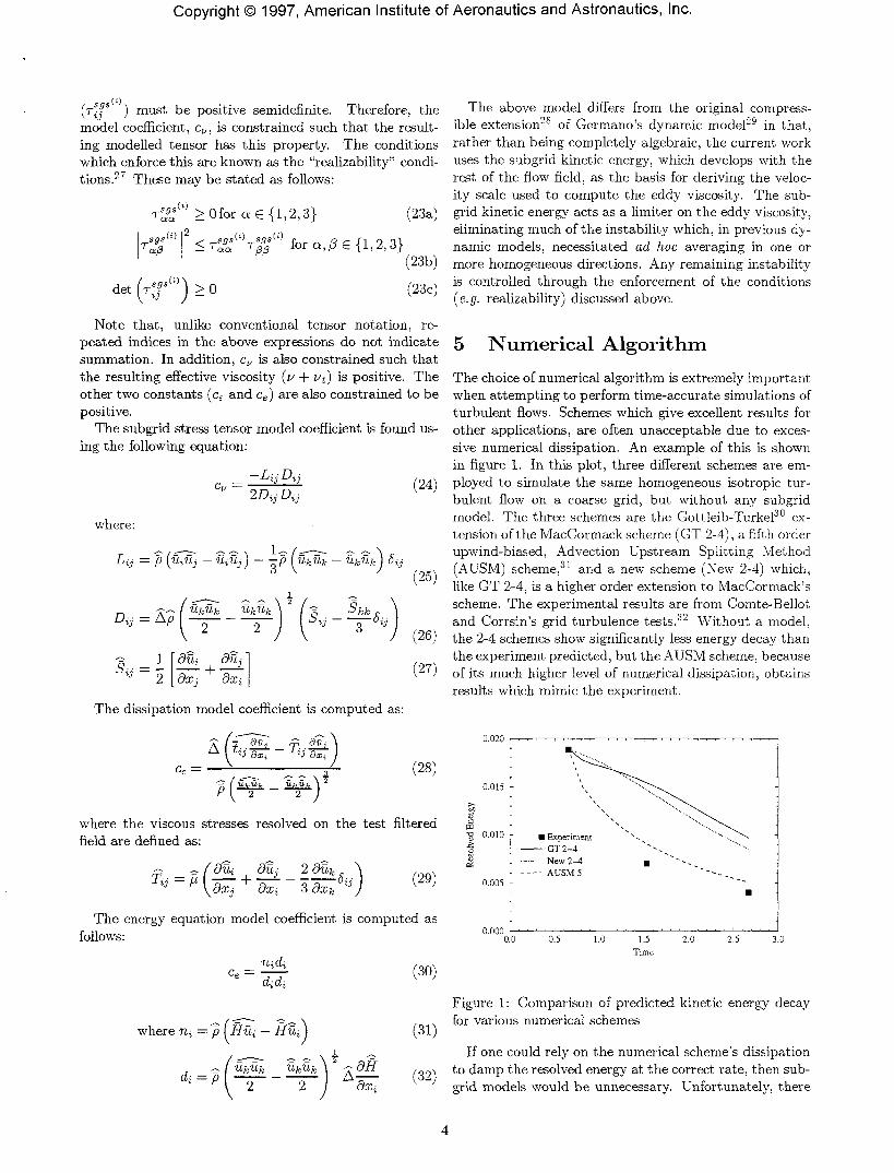
5 Numerical AlgorithmThe choice of numerical algorithm is extremely importantwhen attempting to perform time-accurate simulations ofturbulent flows. Schemes which give excellent results forother applications, are often unacceptable due to exces-sive numerical dissipation. An example of this is shownin figure 1. In this plot, three different schemes are em-ployed to simulate the same homogeneous isotropic tur-bulent flow on a coarse grid, but without any subgridmodel. The three schemes are the Gottleib-Turkel30 ex-tension of the MacCormack scheme (GT 2-4), a fifth orderupwind-biased, Advection Upstream Splitting Method(AUSM) scheme,31 and a new scheme (New 2-4) which,like GT 2-4, is a higher order extension to MacCormack'sscheme. The experimental results are from Comte-Bellotand Corrsin's grid turbulence tests.32 Without a model,the 2-4 schemes show significantly less energy decay thanthe experiment predicted, but the AUSM scheme, becauseof its much higher level of numerical dissipation, obtainsresults which mimic the experiment.
0.020
0.015
1 o.oio
0.005
0.0000.5 1.5
Time2.5 3.0
Figure 1: Comparison of predicted kinetic energy decayfor various numerical schemes
If one could rely on the numerical scheme's dissipationto damp the resolved energy at the correct rate, then sub-grid models would be unnecessary. Unfortunately, there
Copyright© 1997, American Institute of Aeronautics and Astronautics, Inc.
are no guarantees that this will take place. In this case,for example, while the resolved energy is being dissipatedas the solution progresses, AUSM's results do not matchthe experiment. Thus a subgrid model is still necessary. Ifthe cell Reynolds number can be kept low enough, the ef-fects of numerical dissipation will remain sufficiently smallthat the subgrid model can still function. The Reynoldsnumber for this case, for instance, while high enough tomake DNS difficult, is still comparatively low, and thenumerical dissipation has not exceeded the actual dis-sipation observed in the experiment. For a truly highReynolds number flow, however, it is easy to see thatthe dissipation in the AUSM scheme would overwhelmthe viscous and turbulent forces to the extent that nosubgrid model could compensate enough to obtain thecorrect results.
The numerical scheme used for this work is aMac Cor mack-type method similar to the Gottlieb-Turkelmethod.30 In contrast to that method, the current schemeis truly fourth order in space (on a uniform grid) and (likeGottlieb-Turkel) it is second order in time. The algorithmis implemented in a finite volume sense. On stretchedgrids, the algorithm uses an interpolant which attemptsto preserve some of the properties that the scheme has onuniform grids, but the scheme does not remain strictlyfourth order.
6 Model Validation
0.020
0.015 -
•5 0.010 -
0.005 -
0.000
• Experiment——— GT2-4- No Model......... GT2-4- LES- Favre--- New 2-4-No Model— — New 2-1- LES- Favre*- - •* New 2-4- LES- Current
0.5 1.0 1.5Time
2.0 2.5
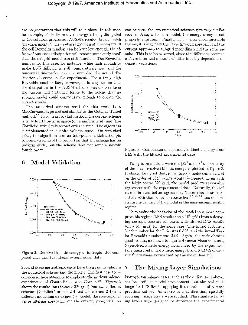
Figure 2: Resolved kinetic energy of isotropic LES com-pared with grid turbulence experimental data
Several decaying isotropic cases have been run to validatethe numerical scheme and the model. The first case to beconsidered here attempts to duplicate the grid-turbulenceexperiments of Comte-Bellot and Corrsin.32 Figure 2shows the results (on the same 323 grid) from two differentschemes (Gottlieb-Turkel's 2-4 and the current 2-4) anddifferent modelling strategies (no model, the conventionalFavre filtering approach, and the current approach). As
can be seen, the two numerical schemes give very similarresults. Also, without a model, the energy decay is notproperly captured. Finally, in the near-incompressibleregime, it is seen that the Favre filtering approach and thecurrent approach to subgrid modelling yield the same re-sults. This is to be expected, since the difference betweena Favre filter and a 'straight' filter is solely dependant ondensity variations.
0.03
0.02
0.01
0.00
•Exp.- 32s
— LES- 32*•Exp.- 48!
••- LES- 48*
0.0 0.5 1.0 1.5Time
2.0 2.5 3.0
Figure 3: Comparison of the resolved kinetic energy fromLES with the filtered experimental data
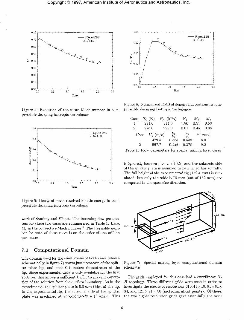
Two grid resolutions were run (323 and 483). The decayof the mean resolved kinetic energy is plotted in figure 3.It should be noted that, for a direct simulation, a grid ofon the order of 3843 points would be needed. Even withthe fairly coarse 323 grid, the model predicts reasonableagreement with the experimental data. Naturally, the 483
case is in even better agreement. These results are con-sistent with those of other researchers10'33'34 and demon-strate the validity of the model in the near-incompressibleregime.
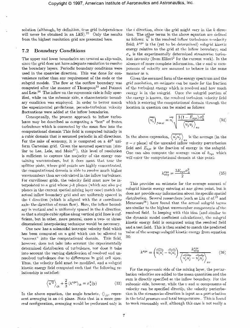
To examine the behavior of the model in a more com-pressible regime, LES results (on a 163 grid) from a decay-ing isotropic case are compared with filtered DNS results(on a 643 grid) for the same case. The initial turbulentMach number for the DNS was 0.826, and the initial Tay-lor Reynolds number was 34.9. Again, the code obtainsgood results, as shown in figures 4 (mean Mach number).5 (resolved kinetic energy normalized by the experimen-tally measured initial kinetic energy), and 6 (RMS of den-sity fluctuations normalized by the mean density).
7 The Mixing Layer SimulationsIsotropic turbulence cases, such as those discussed above,can be useful in model development, but the real chal-lenge for LES lies in applying it to problems of a morepractical nature. As a step in that direction, spatiallyevolving mixing layers were studied. The simulated mix-ing layers were designed to duplicate the experimental
Copyright© 1997, American Institute of Aeronautics and Astronautics, Inc.
0.80
0.5 1.0 1.5 2.0 2.50.00
0.0
Figure 4: Evolution of the mean Mach number in com-pressible decaying isotropic turbulence
i.o
'0.6
I0'4a.
0.2
0.0
— Filtered DNSOie'LES
0.0 0.5 1.0 1.5 2.0 2.5Time
Figure 5: Decay of mean resolved kinetic energy in com-pressible decaying isotropic turbulence
work of Samimy and Elliott. The incoming flow parame-ters for these two cases are summarized in Table 1. Here,Mc is the convective Mach number.5 The Reynolds num-ber for both of these cases is on the order of one millionper meter.
7.1 Computational DomainThe domain used for the simulations of both cases (shownschematically in figure 7) starts just upstream of the split-ter plate lip, and ends 0.4 meters downstream of thelip. Since experimental data is only available for the first250mm, this allows a sufficient buffer to prevent corrup-tion of the solution from the outflow boundary. As in theexperiments, the splitter plate is 0.5 mm thick at the lip.In the experimental rig, the subsonic side of the splitterplate was machined at approximately a 1° angle. This
0.25
0.20
0.15
0.10
0.05
0.00
Filtered DNSOlff'LES
0.0 0.5 1.0 1.5Time
2.0 2.5
Figure 6: Normalized RMS of density fluctuations in com-pressible decaying isotropic turbulence
Case To (K) P01 291.02 276.0
Case U\ (m/s1 479.52 597.7
314.0722.0
0.3550.246
MI1.803.01
PI0.6380.370
M20.510.45
<5
Mc0.530.88
(mm)8.09.2
Table 1: Flow parameters for spatial mixing layer cases
is ignored, however, for the LES, and the subsonic sideof the splitter plate is assumed to be aligned horizontally.The full height of the experimental rig (152.4 mm) is sim-ulated, but only the middle 76 mm (out of 152 mm) arecomputed in the spanwise direction.
0.5
152 mm
Figure 7: Spatial mixing layer computational domainschematic
The grids employed for this case had a curvilinear H-H topology. Three different grids were used in order toinvestigate the effects of resolution: 61 x41 x 18, 91 x 61 x34, and 121 x 91 x 50 (including ghost points). Of these,the two higher resolution grids gave essentially the same
6
Copyright© 1997, American Institute of Aeronautics and Astronautics, Inc.
solution (although, by definition, true grid independencewill never be obtained in an LES).22 Only the resultsfrom the highest resolution grid are presented here.
7.2 Boundary ConditionsThe upper and lower boundaries are treated as slip-walls,since the grid does not have adequate resolution to resolvethe boundary layers. Periodic boundary conditions wereused in the spanwise direction. This was done for con-venience rather than any requirement of the code or thesubgrid models. The flow at the outflow boundary wascomputed after the manner of Thompson35 and Poinsotand Lele.36 The inflow on the supersonic side is fully spec-ified, while on the subsonic side, a characteristic bound-ary condition was employed. In order to better matchthe experimental predictions, pseudo-turbulent velocityfluctuations were added at the inflow boundaries.
Conceptually, the present approach to inflow turbu-lence may be described as computing a "box" of frozenturbulence which is convected by the mean flow into thecomputational domain This field is computed initially ina cubic domain that is assumed periodic in all directions.For the sake of economy, it is computed on a 483 uni-form Cartesian grid. Given the assumed spectrum (sim-ilar to Lee, Lele, and Moin37), this level of resolutionis sufficient to capture the majority of the energy con-taining wavenumbers, but it does mean that near thesplitter plate, where grid points are highly concentrated,the computational domain is able to resolve much higherwavenumbers than are calculated in the inflow turbulence.For curvilinear grids, the velocity field must now be in-terpolated to a grid whose j-k planes (which are also y-zplanes in the current spatial mixing layer case) match theactual inflow boundary grid and are uniformly spaced inthe i direction (which is aligned with the x coordinateaxis- the direction of mean flow). Here, the inflow bound-ary is vertical and is uniformly spaced in the k direction,so that a simple cubic spline along vertical grid lines is suf-ficient, but in other, more general, cases a two- or three-dimensional interpolating technique would be necessary.
One now has a solenoidal isotropic velocity field whichhas been computed on a grid which can be allowed to"convert" into the computational domain. This field,however, does not take into account the experimentallydetermined distribution of turbulence, nor does it takeinto account the varying distribution of resolved and un-resolved turbulence due to differences in grid cell sizes.Thus, the velocity field must be modified, and a subgridkinetic energy field computed such that the following re-lationship is satisfied:
'-m\ 2u •ik
(33)
In the above equation, the angle brackets, 0^, repre-sent averaging in an i-k plane. Note that in a more gen-eral configuration, averaging would be performed only in
the i direction, since the grid might vary in the k direc-tion. The other terms in the above equation are definedas follows: u is the resolved inflow turbulence it-velocityfield; ksgs is the (yet to be determined) subgrid kineticenergy relative to the grid at the inflow boundary; andau is the experimentally determined streamwise turbu-lent intensity (from Elliott2 for the current work). In theabsence of more complete information, the v and w com-ponents of velocity are assumed to behave in the samemanner as u.
Given the assumed form of the energy spectrum and thegrid resolution, an estimate can be made for the fractionof the turbulent energy which is resolved and how muchenergy is in the subgrid. Once the subgrid portion ofthe energy is known, the resolved turbulent velocity fieldwhich is entering the computational domain through thelocation in question can be scaled as follows:
\ —il =ui/ final
(34)
In the above expression, (u-u- } is the average (in the\ J J I xz
x — z plane) of the unsealed inflow velocity perturbationfield and Esgs is the fraction of energy in the subgrid.One can also compute the average value of ksgs whichwill enter the computational domain at this point:
sgs _— (35)
This provides an estimate for the average amount ofsubgrid kinetic energy entering at any given point, but itdoes not provide any information about its specific spatialdistribution. Several researchers (such as Liu et a/.26 andMeneveau38) have found that the actual subgrid termsare similar to the highest wavenumber components of theresolved field. In keeping with this idea (and similar tothe dynamic model coefficient calculations), the subgridkinetic energy field is computed using the resolved fieldand a test field. This is then scaled to match the predictedvalue of the average subgrid kinetic energy from equation36:
(36)
For the supersonic side of the mixing layer, the pertur-bation velocities are added to the mean quantities and thesum is directly specified at the inflow boundary. For thesubsonic side, however, while the v and w components ofvelocity can be specified directly, the velocity perturba-tion in the streamwise direction is input as a perturbationin the total pressure and total temperature.. This is foundto work reasonably well, although this case is not really a
Copyright© 1997, American Institute of Aeronautics and Astronautics, Inc.
fair test, because the high speed side's perturbations areso much larger than the low speed side's that the latterare comparatively insignificant. Indeed, Samimy and El-liott have presented no data on the boundary layers orlevels of turbulence for the low speed side inflow.
7.3 ResultsThe general procedure used for both the cases presentedhere was to run the solver until the initial conditions hadbeen washed out of the domain. At this point (designatedas a single flowthrough time), time averaging was begun.The simulations were then run for four (Mc = 0.86) or five(Mc = 0.51) more flowthrough times. By this time, thetime-averaged statistics were essentially stationary. De-spite the relative coarseness of even the finest grid used inthis study (121x91x50), the results are surprisingly goodwhen compared to experiment. The momentum thicknessas a function of position downstream of the splitter plate,shown in figure 8, is reasonably well captured by the LES.The effect of compressibility is shown in the decrease inthickness (both in the simulation and experiment) for thehigher convective Mach number case.
the freestream values are underpredicted (probably dueto lack of resolution in these areas). As with the exper-iment, the U* profiles showed self-similarity earlier thanthe turbulent quantities, which are not fully similar until150mm, downstream of the splitter plate. For the suc-ceeding plots of turbulent quantities, data is shown onlyfor those measuring stations which are downstream of theonset of self-similar behavior.
Oi=60mra- Exp.O;r=120nirn- Exp.O*=150mni-Exp.A ;c=180mm- Exp.V*=210mm- Exp.
-- ;c=120mn]-LES- ;c=150mm-LES- *=180nim- LES-- *=210mni-LES
-0.2-1.5 -1.0
5.0
4.0
2.0 :
1.0
D Exp.- Af = 0.51— LES-A/= 0.51
O Exp.- A/ = 0.86-- LES-A/= 0.86
50 100 150x (mm)
200 250 300
Figure 8: Comparison of LES predicted momentum thick-ness with the experimental data of Samimy and Elliott
In general, the simulation results for the Mc = 0.51agree very well with experiment. Normalized velocityprofiles for this case at various streamwise stations areplotted in figure 9. The agreement with the experimen-tal data is excellent. As the figure shows, the self-similarcharacter of the mean flow is well resolved by the currentscheme.
Turbulent quantities are also in good agreement withexperiment. Figure 10 shows streamwise turbulent in-tensity profiles at the same locations as for the previousfigure. Both the peak magnitude and the overall distri-bution of turbulence are well predicted compared to theexperiment. The width is correct, as is the shape and theself-similar nature of the profiles. Note, however, that
Figure 9: Normalized mean velocity profiles in the Mc0.51 mixing layer
0.25
-1.5 -1.0 -0.5 0.0 0.5 1.0 1.5
Figure 10: Profiles of streamwise turbulence intensity inthe Mc — 0.51 mixing layer
The lateral turbulence intensity, shown in figure 11, isalso in excellent agreement with experiment. Not onlyare the shape and the width of the profiles in the self-similar region correct, but the magnitude is also correct.The Reynolds stress profiles (u'v'} shown in figure 12, arenot as well resolved. Although the width of the profiles iscorrect and self-similar behavior is predicted, the magni-tudes are significantly higher in the simulation. There areseveral possible sources for this error. It may be a result
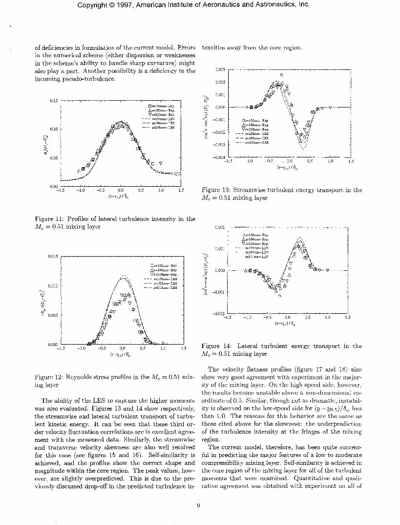
Copyright© 1997, American Institute of Aeronautics and Astronautics, Inc.
of deficiencies in formulation of the current model. Errorsin the numerical scheme (either dispersion or weaknessesin the scheme's ability to handle sharp curvature) mightalso play a part. Another possibility is a deficiency in theincoming pseudo-turbulence.
0.15
tensities away from the core region.
-1.5
0.002
^ 0.001
tT 0.000
"> -0.001avi-~ -0.002
-0.003
-0.004
Ox=150nmi-
V*=210mni-Exp.--- *=150mm-LES
— - - :c=210mni-LES
-1.5 -1.0 -0.5 0.0 0.5'os)/s.
1.5
Figure 13: Streamwise turbulent energy transport in theMc = 0.51 mixing layer
Figure 11: Profiles of lateral turbulence intensity in thelayerMc = 0.51
0.015
0.010
0.005 -
i- Exp.i- Exp.
V*=210nim-Exp.— - - *=150mm- LES— — x=180nmi-LES— - - ^=210rani-LES
0.000_i 5
Figure 12: Reynolds stress profiles in the Mc =0.51 mix-ing layer
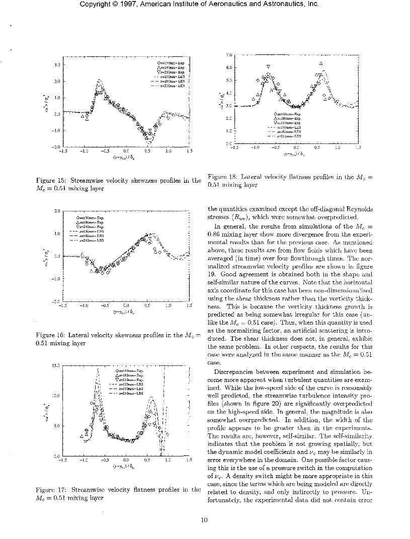
The ability of the LES to capture the higher momentswas also evaluated. Figures 13 and 14 show respectively,the streamwise and lateral turbulent transport of turbu-lent kinetic energy. It can be seen that these third or-der velocity fluctuation correlations are in excellent agree-ment with the measured data. Similarly, the streamwiseand transverse velocity skewness are also well resolvedfor this case (see figures 15 and 16). Self-similarity isachieved, and the profiles show the correct shape andmagnitude within the core region. The peak values, how-ever, are slightly over predicted. This is due to the pre-viously discussed drop-off in the predicted turbulence in-
0.000
-0.001 -
-0.002-1.5
Figure 14: Lateral turbulent energy transport in theMc = 0.51 mixing layer
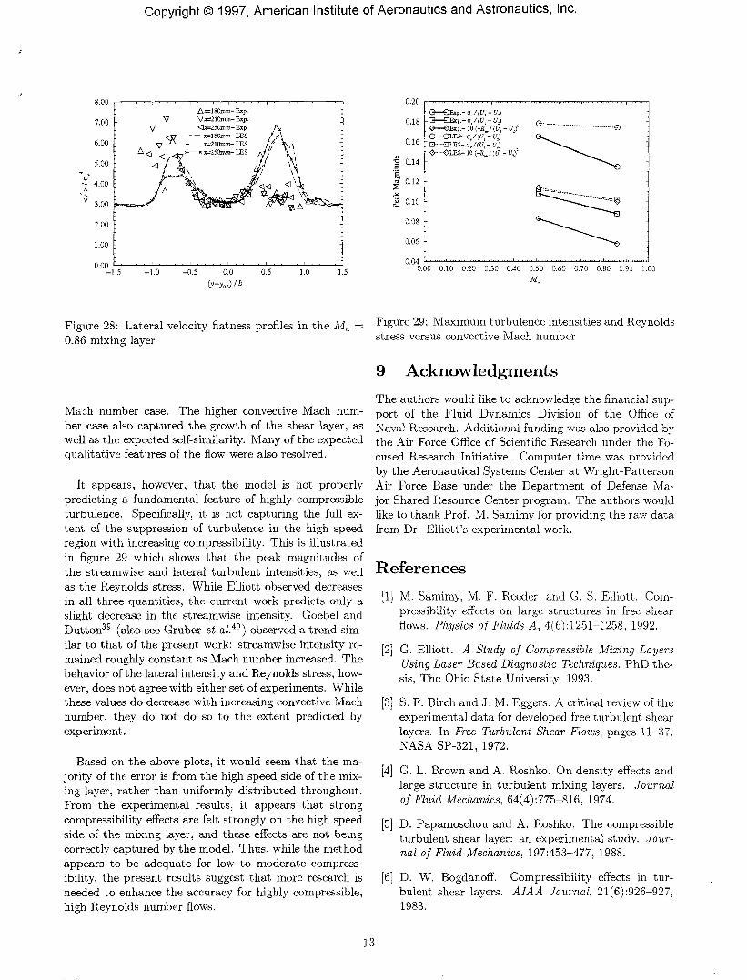
The velocity flatness profiles (figure 17 and 18) alsoshow very good agreement with experiment in the major-ity of the mixing layer. On the high speed side, however,the results become unstable above a non-dimensional co-ordinate of 0.5. Similar, though not as dramatic, instabil-ity is observed on the low-speed side for (y — j/o.s)/^ lessthan 1.0. The reasons for this behavior are the same asthose cited above for the skewness: the underpredictionof the turbulence intensity at the fringes of the mixingregion.
The current model, therefore, has been quite success-ful in predicting the major features of a low to moderatecompressibility mixing layer. Self-similarity is achieved inthe core region of the mixing layer for all of the turbulentmoments that were examined. Quantitative and quali-tative agreement was obtained with experiment on all of
Copyright© 1997, American Institute of Aeronautics and Astronautics, Inc.
3.0 -
2.0 :
V 1.0 :A
-2.0
A*=180mm-Exp. '•Vx=210mni-Exp. :
--- jc=15Qmm-LES— — j*=180mni- LES ^
ni- LES
/ .u
6.0
5.0
4.0
3.0
2.0
1.0
n n
V
°#toA/ ^A o
• ——— " esSe *Oi=150mm-Exp.A*=180mm- Exp.V*=210mm-Exp.
- - - J=150mm- LES— — j=180nmi-LES— -- i=210mra-LES
A
T\\ -7> o \A V,
-
.
-1.5 -1.0 -0.5 0.0 0.5 1.0 1.5-1.5 -0.5 0.5 1.5
Figure 15: Streamwise velocity skewness profiles in theMc = 0.51 mixing layer
Figure 18: Lateral velocity flatness profiles in the Mc =0.51 mixing layer
2.0
1.0
-2.0
O*=150mm- Exp.A*=180mm-Exp.V*=210nmi-Exp.
-- i=150mm-LES-— j=180mm-LES---J=210mra-LES
-1.5 -1.0 -0.5 0.0 0.5 1.0 1.5
Figure 16: Lateral velocity skewness profiles in the Mc0.51 mixing layer
15.0
10.0
5.0
0.0-1.0 -0.5 0.0 0.5 1.0 1.5
Figure 17: Streamwise velocity flatness profiles in theMc = 0.51 mixing layer
the quantities examined except the off-diagonal Reynoldsstresses (Ruv), which were somewhat overpredicted.
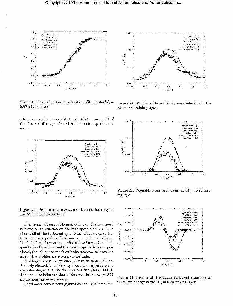
In general, the results from simulations of the Mc =0.86 mixing layer show more divergence from the experi-mental results than for the previous case. As mentionedabove, these results are from flow fields which have beenaveraged (in time) over four flowthrough times. The nor-malized Streamwise velocity profiles are shown in figure19. Good agreement is obtained both in the shape andself-similar nature of the curves. Note that the horizontalaxis coordinate for this case has been non-dimensionalizedusing the shear thickness rather than the vorticity thick-ness. This is because the vorticity thickness growth ispredicted as being somewhat irregular for this case (un-like the Mc = 0.51 case). Thus, when this quantity is usedas the normalizing factor, an artificial scattering is intro-duced. The shear thickness does not, in general, exhibitthe same problem. In other respects, the results for thiscase were analyzed in the same manner as the Mc = 0.51case.
Discrepancies between experiment and simulation be-come more apparent when turbulent quantities are exam-ined. While the low-speed side of the curve is reasonablywell predicted, the Streamwise turbulence intensity pro-files (shown in figure 20) are significantly overpredictedon the high-speed side. In general, the magnitude is alsosomewhat overpredicted. In addition, the width of theprofile appears to be greater than in the experiments.The results are, however, self-similar. The self-similarityindicates that the problem is not growing spatially, butthe dynamic model coefficients and vc may be similarly inerror everywhere in the domain. One possible factor caus-ing this is the use of a pressure switch in the computationof vc. A density switch might be more appropriate in thiscase, since the terms which are being modeled are directlyrelated to density, and only indirectly to pressure. Un-fortunately, the experimental data did not contain error
10
Copyright© 1997, American Institute of Aeronautics and Astronautics, Inc.
0.15
0.10
0.05
Ax^lSOnmi- Exp.V*=21 Omni-Exp.<Cx=250nuu- Exp.
— — ;c=180mm-LES— - - ;t=210nini-LES
:c=250nini- LES
-1.5 -1.0 -0.5 0.0 0.5 1.0 1.5
Figure 19: Normalized mean velocity profiles in the Mc =0.86 mixing layer
Figure 2i: Profiles of lateral turbulence intensity in theMC = 0 86 mixing layer
estimates, so it is impossible to say whether any part ofthe observed discrepancies might be due to experimentalerror.
0.25A*=180mm-ExpVj=2JOmm- Exp<:t=250mro- Exp
— — :c=180nini- LES—-- i=210nim-LES
i=250mm- LES
0.00-1.0 -0.5 0.0 0.5
<y-y,J/i>
0.015Aj=180iuni-ExpV*=210mni-Exp<]*=250mm-Exp
j=180mm-LESi=210mm-LESj=250mm- LES
Figure 22: Reynolds stress profiles in the Mc = 0.86 mix-ing layer
Figure 20: Profiles of streamwise turbulence intensity inthe Mc = 0.86 mixing layer
This trend of reasonable predictions on the low-speedside and overprediction on the high speed side is seen onalmost all of the turbulent quantities. The lateral turbu-lence intensity profiles, for example, are shown in figure21. As before, they are somewhat skewed toward the highspeed side of the flow, and the peak magnitude is overpre-dicted, though not as much as is the streamwise intensity.Again, the profiles are strongly self-similar.
The Reynolds stress profiles, shown in figure 22. aresimilarly skewed, but the magnitude is overpredict ed toa greater degree than in the previous two plots. This issimilar to the behavior that is observed in the A/,: = 0.51simulations, as shown above.
Third order correlations (figures 23 and 24) show a sim-
-0.001
-0.002
-0.003 -
-0.004-1.5
Figure 23: Profiles of streamwise turbulent transport ofturbulent energy in the Mc = 0.86 mixing layer
11
Copyright© 1997, American Institute of Aeronautics and Astronautics, Inc.
0.002
-0.002
A*=180mm-Exp.
0.001 -i- Exp.
— — jr=180mm-LES— - - x=210mm-LES« —— « *=250mm- LES
-o.ooi -
-1.5
2.00
1.00
0.00
-1.00
-2.00
A*=180mm-Exp.V*=210mro-Exp.<]z=250nim-Exp.
— *=180]iim-LES
-1.5 -1.0 -0.5 0.0 0.5 i.o 1.5
Figure 24: Profiles of lateral turbulent transport of tur-bulent energy in the Mc = 0.86 mixing layer
Figure 26: Profiles of lateral velocity skewness in theMc = 0.86 mixing layer
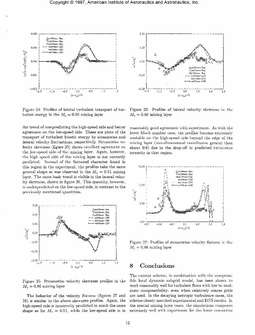
ilar trend of overpredicting the high-speed side and betteragreement on the low-speed side. These are plots of thetransport of turbulent kinetic energy by streamwise andlateral velocity fluctuations, respectively. Streamwise ve-locity skewness (figure 25) shows excellent agreement onthe low-speed side of the mixing layer. Again, however,the high speed side of the mixing layer is not correctlypredicted. Instead of the flattened character found inthis region in the experiment, the profiles take the samegeneral shape as was observed in the Mc = 0.51 mixinglayer. The same basic trend is visible in the lateral veloc-ity skewness, shown in figure 26. This quantity, however,is underpredicted on the low-speed side, in contrast to thepreviously mentioned quantities.
3.00
2.00 r <;c=250mm-Exp— — j=180mm-LES— - - z=210mro-LES
j=250ram- LES
-2.00 r
-3.00-1.5
Figure 25: Streamwise velocity skewness profiles in theMc = 0.86 mixing layer
The behavior of the velocity flatness (figures 27 and28) is similar to the above skewness profiles. Again, thehigh-speed side is incorrectly predicted in much the sameshape as for Mc = 0.51, while the low-speed side is in
reasonably good agreement with experiment. As with thelower Mach number case, the profiles become extremelyunstable on the high-speed side beyond the edge of themixing layer (non-dimensional coordinates greater thanabout 0.6) due to the drop-off in predicted turbulenceintensity in that region.
15.00
10.00
5.00
0.00
ta\!
Vj=210mm-Exp.<j=250mm- Exp.
— — j=180mm- LES— - - -i=210mm-LESi———:jc250mm-LES
-1.5 -1.0 -0.5 0.0 0.5(y-y^'b
Figure 27: Profiles of streamwise velocity flatness in theMc = 0.86 mixing layer
8 ConclusionsThe current scheme, in combination with the compress-ible local dynamic subgrid model, has been shown towork reasonably well for turbulent flows with low to mod-erate compressibility- even when relatively coarse gridsare used. In the decaying isotropic turbulence cases, thescheme closely matched experimental and DNS results. Inthe spatial mixing layer cases, the simulations comparedextremely well with experiment for the lower convective
12
Copyright© 1997, American Institute of Aeronautics and Astronautics, Inc.
8.00
7.00
6.00
S.OO
4.00
3.00
2.00
1.00
0.00-1
- Exp.V*=210nini-E:<p.<k=250mm- Exp.
-— ;c=180mm-LES--- x=210mm-LES
«x=250mm- LES
0.20
0.18
0.16
| 0.14I Q12
| 0.10
0.08
0.06 -
'-B—HExp.-o./fU.-Cy; O——OExp.- 10 (-R./I.U,
&•••• OLES- 0,/fu, - yjQ---DLES- a,/(Ul - U^
• O---OLES- 10 (-fl./W
-0.5 0.5 i.o 1.5 0.00 0.10 0.20 0.30 0.40 0.50 0.60 0.70 0.80 0.90 1.00M,
Figure 28: Lateral velocity flatness profiles in the Mc = FiSure 29: Maximum turbulence intensities and Reynolds0.86 mixing layer
Mach number case. The higher convective Mach num-ber case also captured the growth of the shear layer, aswell as the expected self-similarity. Many of the expectedqualitative features of the flow were also resolved.
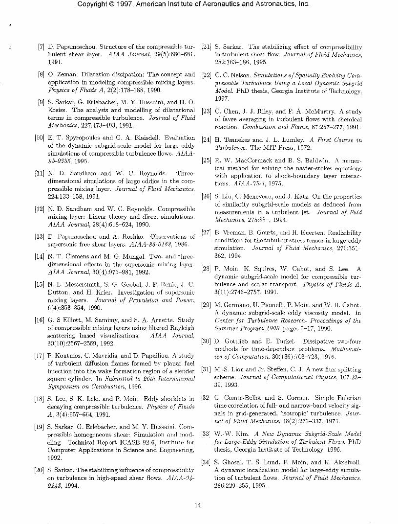
It appears, however, that the model is not properlypredicting a fundamental feature of highly compressibleturbulence. Specifically, it is not capturing the full ex-tent of the suppression of turbulence in the high speedregion with increasing compressibility. This is illustratedin figure 29 which shows that the peak magnitudes ofthe streamwise and lateral turbulent intensities, as wellas the Reynolds stress. While Elliott observed decreasesin all three quantities, the current work predicts only aslight decrease in the streamwise intensity. Goebel andButton39 (also see Gruber et a^.40) observed a trend sim-ilar to that of the present work: streamwise intensity re-mained roughly constant as Mach number increased. Thebehavior of the lateral intensity and Reynolds stress, how-ever, does not agree with either set of experiments. Whilethese values do decrease with increasing convective Machnumber, they do not do so to the extent predicted byexperiment.
Based on the above plots, it would seem that the ma-jority of the error is from the high speed side of the mix-ing layer, rather than uniformly distributed throughout.From the experimental results, it appears that strongcompressibility effects are felt strongly on the high speedside of the mixing layer, and these effects are not beingcorrectly captured by the model. Thus, while the methodappears to be adequate for low to moderate compress-ibility, the present results suggest that more research isneeded to enhance the accuracy for highly compressible,high Reynolds number flows.
stress versus convective Mach number
9 AcknowledgmentsThe authors would like to acknowledge the financial sup-port of the Fluid Dynamics Division of the Office ofNaval Research. Additional funding was also provided bythe Air Force Office of Scientific Research under the Fo-cused Research Initiative. Computer time was providedby the Aeronautical Systems Center at Wright-PattersonAir Force Base under the Department of Defense Ma-jor Shared Resource Center program. The authors wouldlike to thank Prof. M. Samimy for providing the raw datafrom Dr. Elliott's experimental work.
References[1] M. Samimy, M. F. Reeder, and G. S. Elliott. Com-
pressibility effects on large structures in free shearflows. Physics of Fluids A, 4(6):1251-1258, 1992.
[2] G. Elliott. A Study of Compressible Mixing LayersUsing Laser Based Diagnostic Techniques. PhD the-sis, The Ohio State University, 1993.
[3] S. F. Birch and J. M. Eggers. A critical review of theexperimental data for developed free turbulent shearlayers. In Free Turbulent Shear Flows, pages 11-37.NASA SP-321, 1972.
[4] G. L. Brown and A. Roshko. On density effects andlarge structure in turbulent mixing layers. Journalof Fluid Mechanics, 64(4): 775-816, 1974.
[5] D. Papamoschou and A. Roshko. The compressibleturbulent shear layer: an experimental study. Jour-nal of Fluid Mechanics, 197:453-477, 1988.
[6] D. W. Bogdanoff. Compressibility effects in tur-bulent shear layers. AIAA Journal, 21(6):926-927,1983.
13
Copyright© 1997, American Institute of Aeronautics and Astronautics, Inc.
[7] D. Papamoschou. Structure of the compressible tur-bulent shear layer. AIAA Journal, 29(5):680-681,1991.
[8] 0. Zeman. Dilatation dissipation: The concept andapplication in modeling compressible mixing layers.Physics of Fluids A, 2(2):178-188, 1990.
[9] S. Sarkar, G. Erlebacher, M. Y. Hussaini, and H. 0.Kreiss. The analysis and modelling of dilatationalterms in compressible turbulence. Journal of FluidMechanics, 227:473-493, 1991.
[10] E. T. Spyropoulos and G. A. Blaisdell. Evaluationof the dynamic subgrid-scale model for large eddysimulations of compressible turbulence flows. AIAA-95-0355, 1995.
[11] N. D. Sandham and W. C. Reynolds. Three-dimensional simulations of large eddies in the com-pressible mixing layer. Journal of Fluid Mechanics,224:133-158, 1991.
[12] N. D. Sandham and W. C. Reynolds. Compressiblemixing layer: Linear theory and direct simulations.AIAA Journal, 28(4):618-624, 1990.
[13] D. Papamoschou and A. Roshko. Observations ofsupersonic free shear layers. AIAA-86-0162, 1986.
[14] N. T. Clemens and M. G. Mungal. Two- and three-dimensional effects in the supersonic mixing layer.AIAA Journal, 30(4).-973-981, 1992.
[15] N. L. Messersmith, S. G. Goebel, J. P. R.enie, J. C.Button, and H. Krier. Investigation of supersonicmixing layers. Journal of Propulsion and Power,6(4):353-354, 1990.
[16] G. S Elliott, M. Samimy, and S. A. Arnette. Studyof compressible mixing layers using filtered Rayleighscattering based visualizations. AIAA Journal,30(10) :2567-2569, 1992.
[17] P. Koutmos, C. Mavridis, and D. Papailiou. A studyof turbulent diffusion flames formed by planar fuelinjection into the wake formation region of a slendersquare cylinder. In Submitted to 26th InternationalSymposium on Combustion, 1996.
[18] S. Lee, S. K. Lele, and P. Moin. Eddy shocklets indecaying compressible turbulence. Physics of FluidsA, 3(4):657-664, 1991.
[19] S. Sarkar, G. Erlebacher, and M. Y. Hussaini. Com-pressible homogeneous shear: Simulation and mod-eling. Technical Report ICASE 92-6, Institute forComputer Applications in Science and Engineering.1992.
[20] S. Sarkar. The stabilizing influence of compressibilityon turbulence in high-speed shear flows. AIAA-94-2243, 1994.
[21] S. Sarkar. The stabilizing effect of compressibilityin turbulent shear flow. Journal of Fluid Mechanics,282:163-186, 1995.
[22] C. C. Nelson. Simulations of Spatially Evolving Com-pressible Turbulence Using a Local Dynamic SubgridModel. PhD thesis, Georgia Institute of Technology,1997.
[23] C. Chen, J. J. Riley, and P. A. McMurtry. A studyof favre averaging in turbulent flows with chemicalreaction. Combustion and Flame, 87:257-277, 1991.
[24] H. Tennekes and J. L. Lumley. A First Course inTurbulence. The MIT Press, 1972.
[25] R. W. MacCormack and B. S. Baldwin. A numer-ical method for solving the navier-stokes equationswith application to shock-boundary layer interac-tions. AIAA-75-1, 1975.
[26] S. Liu, C. Meneveau, and J. Katz. On the propertiesof similarity subgrid-scale models as deduced frommeasurements in a turbulent jet. Journal of FuidMechanics, 275:85-, 1994.
[27] B. Vreman, B. Geurts, and H. Kuerten. Realizibilityconditions for the tubulent stress tensor in large-eddysimulation. Journal of Fluid Mechanics, 276:351-362, 1994.
[28] P. Moin, K. Squires, W. Cabot, and S. Lee. Adynamic subgrid-scale model for compressible tur-bulence and scalar transport. Physics of Fluids A,3(ll):2746-2757, 1991.
[29] M. Germane, U. Piomelli, P. Moin, and W. H. Cabot.A dynamic subgrid-scale eddy viscosity model. InCenter for Turbulence Research- Proceedings of theSummer Program 1990, pages 5-17. 1990.
[30] D. Gottlieb and E. Turkel. Dissipative two-fourmethods for time-dependant problems. Mathemat-ics of Computation, 30(136):703-723, 1976.
[31] M.-S. Liou and Jr. Steffen, C. J. A new flux splittingscheme. Journal of Computational Physics, 107:23-39, 1993.
[32] G. Comte-Bellot and S. Corrsin. Simple Euleriantime correlation of full- and narrow-band velocity sig-nals in grid-generated, 'isotropic' turbulence. Jour-nal of Fluid Mechanics, 48(2):273-337, 1971.
[33] W.-W. Kim. A New Dynamic Subgrid-Scale Modelfor Large-Eddy Simulation of Turbulent Flows. PhDthesis, Georgia Institute of Technology, 1996.
[34] S. Ghosal, T. S. Lund, P. Moin, and K. Akselvoll.A dynamic localization model for large-eddy simula-tion of turbulent flows. Journal of Fluid Mechanics,286:229-255, 1995.
14
Copyright© 1997, American Institute of Aeronautics and Astronautics, Inc.
[35] K. W. Thompson. Time-dependant boundary condi-tions for hyperbolic systems, II. Journal of Compu-tational Physics, 89:439-461, 1990.
[36] T. J. Poinsot and S. K. Lele. Boundary conditionsfor direct simulations of compressible viscous flows.Journal of Computational Fluids, 101:104-129, 1992.
[37] S. Lee, S. K. Lele, and P. Moin. Simulation of spa-tially evolving turbulence and the applicability ofTaylor's hypothesis in compressible flow. Physics ofFluids A, 4(7):1521-1530, 1992.
[38] C. Meneveau. Statistics of turbulence subgrid-scale stresses: Necessary conditions and experimen-tal tests. Physics of Fluids, 6(2):815-833, 1994.
[39] S. G. Goebel and J. C. Dutton. Experimental studyof compressible turbulent mixing layers. AIAA Jour-nal, 29(4):538-546, 1991.
[40] M. R. Gruber, N. L. Messersmith, and J. C. Dut-ton. Three-dimensional velocity field in a compress-ible mixing layer. AIAA Journal, 31(11):2061-2067,1993.
15


![Theoretical solutions for unsteady compressible … · Theoretical solutions for unsteady compressible subsonic ... (with applications in aeroelasticity) ... Fung [41], Bisplinghoff](https://img.pdfslide.us/doc/110x75/5b0474227f8b9a0a548d9ac0/theoretical-solutions-for-unsteady-compressible-solutions-for-unsteady-compressible.jpg)