confocal_resonator5

7/29/2019 confocal_resonator5

http://slidepdf.com/reader/full/confocalresonator5 1/13

EUROPEAN ORGANIZATION FOR NUCLEAR RESEARCH

CERN - AB DIVISION

CTF3 Note 060 (Tech.)

AB-Note-2003-081 (ABP)TSL-Note-2003-56

Analytical Design of a Confocal Resonator

T. Lofnes, V. Ziemann (Ed.), The Svedberg Laboratory, Uppsala, Sweden

A. Ferrari, Department of Radiation Sciences, Uppsala University, Sweden

ABSTRACT

A confocal resonator may be used as a pick-up for frequencies in the multi-GHzregion, in order to monitor the bunch spacing and/or the bunch length in theCTF3 drive beam. In this note, we collect some formulae regarding the design of aconfocal resonator in order to facilitate the estimation of relevant parameters in a

later more careful numerical study.

Geneva, Switzerland

October 14, 2003



1 Introduction

During the operation of the CLIC Test Facility CTF3 Preliminary Phase, a newmethod was tested to monitor the bunch frequency multiplication in the combiner ring. Acoaxial pick-up and its read-out electronics were designed and mounted in the CTF3 ringin 2002 to allow comparison of the amplitudes of five harmonics of the fundamental beam

frequency (3 GHz) while combining bunch trains. The commissioning of this monitor wasa successful proof of principle for this new method [1, 2]. However, two limitations wereidentified. The first one was that the rise time of the read-out electronics was longer thanthe time extension of the bunch trains (about 6.6 ns). In the next stages of CTF3, thebunch trains will be 140 ns long and this limitation will thus disappear. The second limita-tion was the presence of waveguide modes, which were excited by discontinuities upstreamin the beam pipe and which were propagating in the wake of the electron bunches, leadingto a distorsion of the signal coming out from the monitor. The electromagnetic field thatthe bunches carry with them is a quasi-TEM mode, while the other travelling waveguidemodes are TE or TM fields. It was suggested earlier that a confocal resonator like pick-upcould discriminate between the quasi-TEM mode of the beam and the parasitic TE andTM fields [3].

In this note, we make analytical investigations of the geometry, the electromagneticfields and the Q−value of such a device, by using equations that we found in the literature,in order to get some order of magnitude estimates, which will then allow to guide us inlater numerical studies. Here, we focus on a confocal resonator for microwaves with awavelength of 20 mm, which corresponds to a frequency of 15 GHz. We believe that sucha device should be easy to manufacture and test. However, this restriction is not crucial,because all quantities with the dimension of a length directly scale with the wavelength.The corresponding linear dimensions for a 100 GHz resonator would simply be smallerby a factor 100/15. Other quantities that such as Q−values may change, however, by a

different amount.In section 2, we give a review of the equations describing the electromagnetic fieldsin a confocal resonator, with emphasis on the fundamental mode. Then, in section 3, wecompute the various losses of such a cavity. Section 4 aims at optimizing the geometryof the confocal resonator at 15 GHz. In sections 5 and 6, we discuss the coupling of theresonator to the quasi-TEM field of the bunched beam and to the waveguide modespropagating in the beam pipe, respectively. Finally, conclusions are drawn in section 7.

2 Confocal Resonator

The fields in a confocal optical resonator were originally investigated in the early1960s when the first laser oscillators in the microwave and optical regimes appeared. Oneof the first papers was written by Fox and Li [4] and, later, various authors developed thetheory further. A very readable tutorial is given in [5] and an overview of the formulaecan be found in [6], which we will closely follow in this report.

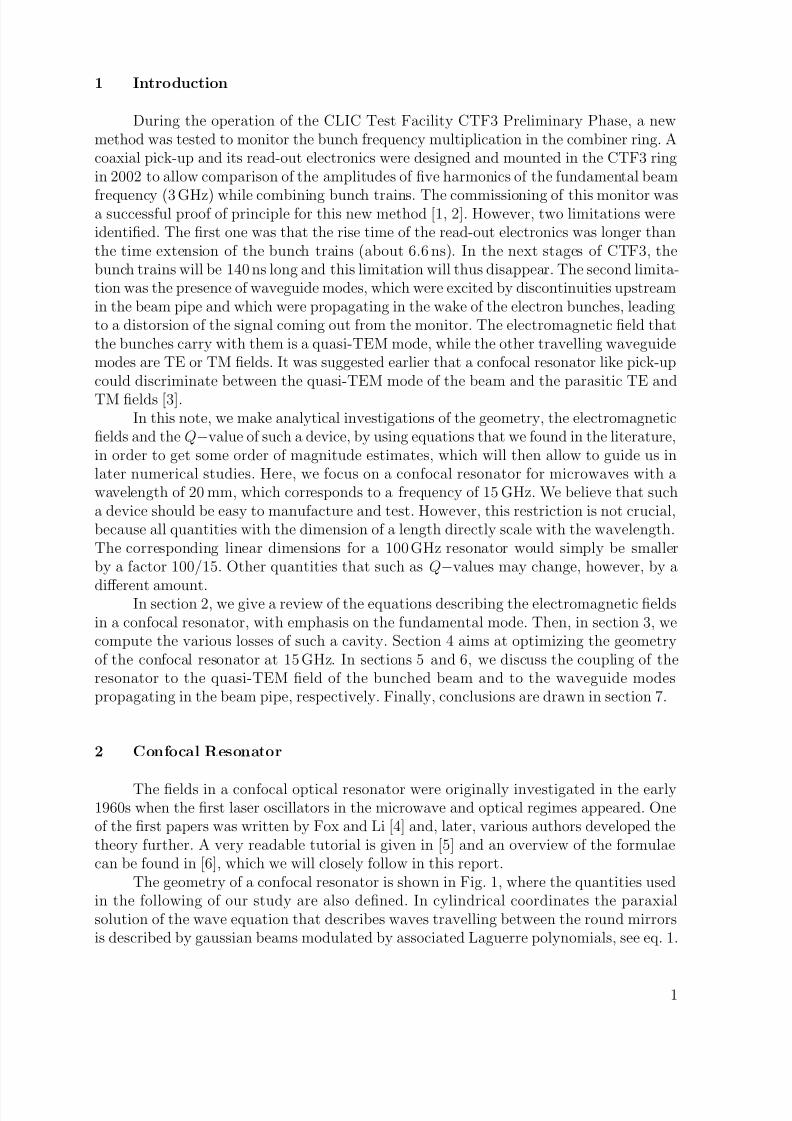
The geometry of a confocal resonator is shown in Fig. 1, where the quantities usedin the following of our study are also defined. In cylindrical coordinates the paraxialsolution of the wave equation that describes waves travelling between the round mirrorsis described by gaussian beams modulated by associated Laguerre polynomials, see eq. 1.

1



z

x

R

D

A

Beam direction

Figure 1: Geometry of a confocal resonator with a definition of the used quantities.

u(r,φ,z ) = A(r,φ,z )exp

−i

kz +

kr2

2R(z )−Θ(z )

A(r,φ,z ) =w0

w(z )

r

w(z )

m

Lmn

2r2

w2(z )

exp

− r2

w2(z )

cos(mφ)

w2(z ) = w20

1 +

z

z 0

2

R(z ) = z

1 +

z 0z

2

(1)

Θ(z ) = (1 + 2n + m) arctan

z z 0

z 0 =kw2

0

2= Rayleigh length

k =2π

λ

where w0 is the waist radius of the optical mode, Lmn is the associated Laguerre polynomial,

and λ is the wavelength. Note that the fundamental mode with n = m = 0 is gaussiantransversely with a rms width w(z )/

√ 2. Here, we choose the coordinate system such that

the waist is at z = 0.

2



In our design we choose the resonator to be confocal, which means that the distanceD between the mirrors is equal to their radius of curvature R, which is also approximatelythe radius of curvature of the wave fronts. In order to have vanishing fields on the mirrorswe require that the cosine of the phase factor vanishes. For the fundamental n = m = 0mode and r = 0 this condition leads to

l +

1

2

π = kz −Θ(z ) = kz − arctan z

z 0

at z = D/2 (2)

where l is an integer. Solving for the mirror distance D at r = 0 we obtain

D =

l +3

4

λ . (3)

If we choose for example l = 3 we obtain a mirror distance of 75 mm, for a wavelength of 20 mm. The choice of this value is motivated more clearly further in this paper.

Having found the distance D between the mirrors and also the radius R = D, wecan calculate the minimum waist w0 from

w20 =

Dλ

2π. (4)

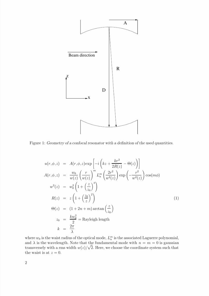
For our configuration, w0 is 15.45 mm, which is of the same order as the wavelength λ.Having estimated all parameters needed in order to calculate the electric field and

the intensities in various planes, we start by plotting the electric field along the z −axis inFig. 2. We observe that the electric field vanishes at the ends i.e. z = ±37.5 mm, wherethe mirrors are located, as expected.

−40 −20 0 20 40

z [mm]

−1

−0.5

0

0.5

1

E l e c t r i c

F i e l d

[ a . u . ]

Figure 2: Electric field on axis, where the mirrors are on the left-hand side and on the right-hand side.

3



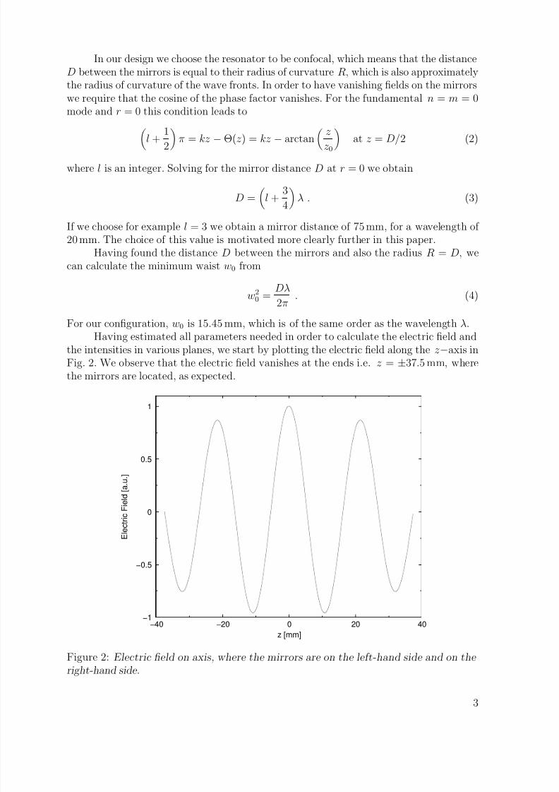
Figure 3: Intensity of the (0,0) mode in the x-z plane, horizontal=x, vertical=z. The area covered is ±40 mm in either direction. The mirrors are at the top and at the bottom.

In Fig. 3 we show the intensity distribution (i.e. the squared electric field) in the

x − z plane. The mirrors are at the top and at the bottom, and the z −axis goes fromtop to bottom. The horizontal direction corresponds to the x−coordinate, which coincideswith the variable r in eq. 1. The intensity maxima are clearly visible and there is one onaxis. The geometry of the confocal resonator with its two half-domes perpendicular tothe direction of the beam together with the modal pattern shown in Fig. 3 makes it clearthat the resonator modes are a sort of trapped modes, which are excited by the passingbeam.

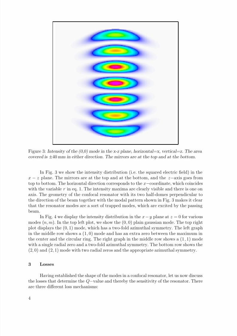
In Fig. 4 we display the intensity distribution in the x−y plane at z = 0 for variousmodes (n, m). In the top left plot, we show the (0, 0) plain gaussian mode. The top rightplot displays the (0, 1) mode, which has a two-fold azimuthal symmetry. The left graph

in the middle row shows a (1, 0) mode and has an extra zero between the maximum inthe center and the circular ring. The right graph in the middle row shows a (1, 1) modewith a single radial zero and a two-fold azimuthal symmetry. The bottom row shows the(2, 0) and (2, 1) mode with two radial zeros and the appropriate azimuthal symmetry.

3 Losses

Having established the shape of the modes in a confocal resonator, let us now discussthe losses that determine the Q−value and thereby the sensitivity of the resonator. Thereare three different loss mechanisms:

4



Figure 4: Intensity distribution in the z=0 plane for the following modes:(0,0),(0,1),(1,0),(1,1),(2,0),(2,1). The distance covered is ±40 mm in either direction.

5



– Diffraction losses,– Losses due to output coupling,– Losses due to finite conductivity.

We start by discussing the diffraction losses. Intuitively, they come from rays that missthe mirrors, if they have a finite extension. These losses are determined by the ratio of the gaussian beam waist w(D/2) on the mirror and the mirror radius A. From eq. 1 we

have w(D/2) =

Dλ/π. Indeed, the relevant parameter for the diffraction losses is theFresnel number N F . For a confocal mirror, it is given by

N F =A2

Dλ= π

A

w(D/2)

2

. (5)

The fractional power loss per mirror αd for the (0, 0) mode is given in terms of theFresnel number by

αd = 16π2N F e−4πN F . (6)

Fig. 3 shows how αd varies as a function of N F and it is clear that we need a Fresnel

number around unity in order to have sufficiently small losses1)

. For N F = 1 we derivea mirror radius of A = √ Dλ = 39 mm. For this value we get αd = 5.5 × 10−4. Thecorresponding Qd−value is given by

Qd =2πD

αdλ= 4.3× 104 . (7)

Following [6] further, and still for the (0,0) mode only, we calculate the losses due toa small central coupling hole used to extract power from the resonator for signal detection.We assume that the mirror has a thickness t and that the hole has a diameter d. Theattenuation in the coupling hole is thus given by

αct =

3.682t

d

2 −

2πt

λ

2

. (8)

The extracted power is inversely proportional to

Qc =27

8π2

λ4D2

d6e2r

2

0/w2

0e2αct (9)

where r0 is the offset of the coupling hole from the center. This implies that the extractedpower is determined by the sixth power of the hole diameter. Larger holes are obviouslyadvantageous to increase the power transmitted to the detector. However, the extracted

power will be missing inside the cavity. The corresponding Qh−value reduces to

Qh =Qc

2e2αct − 1. (10)

There are thus two conflicting requirements. On the one hand, we want to have a largesignal to detect but, on the other hand, we want to keep the Qh−value as large as possiblein order to maximize the sensitivity.

1) Note that eq. 6 strongly resembles the equation for the lifetime of a gaussian electron beam in thepresence of limiting apertures, which depends in a similar way on the ratio of the beam size and theaperture limit.

6



0 0.2 0.4 0.6 0.8 1 1.2 1.4

Fresnel Number N_F

0

0.5

1

f r a c t i o n a l p o w e r l o s s p e

r b o u n c e

Figure 5: Fractional power loss αd as a function of the Fresnel number N F .

Inserting numbers from the previous example and assuming a central hole at r0 = 0with a diameter d = 3 mm and a depth t = 2 mm, we find an attenuation of αct = 2.4, aQc−value of Qc = 1.2× 107 and a total Qh−value of Qh = 1.1× 105.

Then, we have to consider the losses due to a finite conductivity. According to [6],they are determined by a geometry factor characterized by a resistance value

G = Z 0π

2

D

λ(11)

where Z 0 = 377 Ω is the impedance of free space. For our configuration, G = 2200Ω. Theother ”ingredient” is the surface resistivity of the material Rs = 1/σδ, where σ is theconductance of the material and δ is the skin depth. For copper, σ = 5.8× 107/Ωm and,at 15 GHz, the skin depth is 3.8 × 10−7 m. This yields Rs = 0.039Ω. The correspondingQr−value is then given by

Qr =G

Rs= 5.7× 104 . (12)

Note that this result is the same for the fundamental and high-order modes. Since lossesare described by the inverse of the Q−values, it is natural to combine the individualQ−values by adding their inverses, in order to obtain the total Q−value which is about2× 104. Note that this result is the same for the fundamental and high-order modes.

The high Q−value will make the tolerances of the resonator quite tight, becausewe have ∆λ/λ ≈ 1/Q and this corresponds to a change of the mirror distance D byabout 2 µm. Thermal variations could easily distort the resonator by this amount andmay warrant a feedback system to keep the resonator dimensions constant. We need toaddress this more carefully later.2)

2) Thanks to F. Caspers for pointing our attention to this.

7



A

dD

h

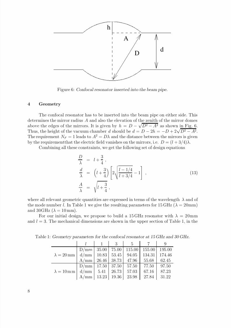
Figure 6: Confocal resonator inserted into the beam pipe.

4 Geometry

The confocal resonator has to be inserted into the beam pipe on either side. Thisdetermines the mirror radius A and also the elevation of the zenith of the mirror domesabove the edges of the mirrors. It is given by h = D −

√ D2 −A2 as shown in Fig. 6.

Thus, the height of the vacuum chamber d should be d = D − 2h = −D + 2√

D2 − A2.The requirement N F = 1 leads to A2 = Dλ and the distance between the mirrors is givenby the requirementthat the electric field vanishes on the mirrors, i.e. D = (l + 3/4)λ.

Combining all these constraints, we get the following set of design equations

D

λ= l +

3

4,

d

λ =

l +3

4

2 l

−1/4

l + 3/4 − 1

, (13)

A

λ=

l +

3

4,

where all relevant geometric quantities are expressed in terms of the wavelength λ and of the mode number l. In Table 1 we give the resulting parameters for 15 GHz (λ = 20mm)and 30GHz (λ = 10 mm).

For our initial design, we propose to build a 15 GHz resonator with λ = 20mmand l = 3. The mechanical dimensions are shown in the upper section of Table 1, in the

Table 1: Geometry parameters for the confocal resonator at 15 GHz and 30 GHz.

l 1 3 5 7 9D/mm 35.00 75.00 115.00 155.00 195.00

λ = 20 mm d/mm 10.83 53.45 94.05 134.31 174.46A/mm 26.46 38.73 47.96 55.68 62.45D/mm 17.50 37.50 57.50 77.50 97.50

λ = 10 m m d/mm 5.41 26.73 57.03 67.16 87.23A/mm 13.23 19.36 23.98 27.84 31.22

8



Resonator

Antenna

Coupling Hole

Terminal

Figure 7: The simple model used to analyze the coupling of the resonator to the antenna.

column labelled 3. We choose a small l in order to maximize the transit time factor forthe coupling to the beam. Another guiding principle was to keep the vacuum chamber assmooth as possible such that the resonator dome simply appears as a weak extrusion fromthe vacuum chamber. Finally the diameter of the dome should not dramatically exceedthe height of the vacuum chamber to avoid excessive tapering of the vacuum chamber in

order to accomodate for the confocal resonator.

5 Coupling to the beam

In this section, we calculate the transfer impedance from the beam current to thevoltage detected at the terminal of the antenna. For this purpose, let us consider thecorresponding kicker model and let us calculate the voltage seen by the beam for a givencurrent oscillating in the antenna. Reciprocity then guarantees that the impedance derivedfor this kicker is equal to the transfer impedance [7, 8].

For definiteness sake, we consider a geometry in which the fields are excited by an

antenna connected to a coaxial line. We consider a simplified model in which the antennais situated in a rectangular waveguide with transverse dimensions a and b, that is coupledthrough a hole with radius r0 to a resonator made up of the same waveguide and closed onthe right-hand side. The corresponding layout is shown in Fig. 7. Note that the waveguideis open on the left-hand side. In this geometry, the radiated power P a from the antennatowards one side of the waveguide is given by [9]

P a =b

2a

Z 0I 2 1− (λ/2a)2

(14)

where λ is the free space wavelength of the radiation and I is the current that drives theantenna. The microwaves emanating from the antenna will eventually meet the couplinghole of radius r0 which, according to [9], can be modelled by a shunt inductance with animpedance

Z hole = Z w2βαm

ab= Z w

8βr30

3ab, (15)

where β =

k20 − (π/a)2 is the propagation constant of the TE01 mode, Z w is the

impedance of the waveguide, and αm = 4r30/3 is the magnetic polarization of a roundcoupling hole. The radius of the coupling hole r0 can be chosen optimally by requir-ing that the impedance of the combined system (resonator + hole) is matched to the

9



impedance of the waveguide Z w and is therefore given by [9]

r30 =3

16π

abλ

1− (λ/2a)2

π

2Q. (16)

In that case, all the energy radiated by the antenna is actually taken up by the resonator.Because of the finite Q

−value, which accounts for the energy loss in the resonator, the

energy does not pile up indefinitely inside the resonator.In order to derive the order of magnitude for the involved quantities, we assume

that the waveguide which is linked to the confocal resonator through the coupling holehas a quadratic cross section with a transverse length a = b = 15mm, and thus abovethe cutoff for 20 mm microwaves. For the resonator, we use the Q−value of 20 000 foundin section 3. For the optimum radius of the coupling hole, we obtain r0 = 1.6 mm whichis close to the value assumed in section 3 where the hole had a diameter of 3 mm.

The power coupled into the resonator will increase the total energy in the resonatorU, which is approximately given by

U =ε02 V E 2dV ≈

πε04 Dw20E 20 , (17)

where E 0 is the electric field on the beam axis and w0 is the waist radius defined insection 2. The amount of energy that escapes the resonator is given by the Q−value suchthat we can write an energy balance for the total energy U in the confocal resonator

dU

dt= −ω

QU + P a . (18)

At the equilibrium we have dU/dt = 0 and U = QP a/ω. Using eq. 17 and solving for theelectric field on the beam axis E 0 we find

E 20 =2Q

π

Z 0I

(l + 3/4)λ

2b/a

1− (λ/2a)2(19)

where we expressed D and w0 in terms of λ and l. Taking the square root we get

E 0 =

2Q

π

Z 0I

(l + 3/4)λ

b

a

1

[1− (λ/2a)2]1/4, (20)

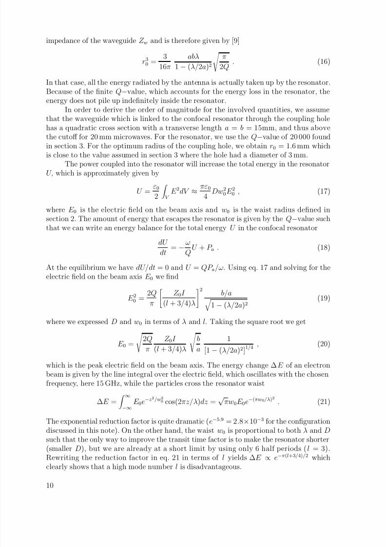
which is the peak electric field on the beam axis. The energy change ∆E of an electronbeam is given by the line integral over the electric field, which oscillates with the chosen

frequency, here 15 GHz, while the particles cross the resonator waist

∆E = ∞

−∞

E 0e−z2/w2

0 cos(2πz/λ)dz =√

πw0E 0e−(πw0/λ)2 . (21)

The exponential reduction factor is quite dramatic (e−5.9 = 2.8×10−3 for the configurationdiscussed in this note). On the other hand, the waist w0 is proportional to both λ and Dsuch that the only way to improve the transit time factor is to make the resonator shorter(smaller D), but we are already at a short limit by using only 6 half periods ( l = 3).Rewriting the reduction factor in eq. 21 in terms of l yields ∆E ∝ e−π(l+3/4)/2 whichclearly shows that a high mode number l is disadvantageous.

10



Finally, the transfer impedance Z t can be deduced by inserting the peak electricfield E 0 from eq. 20 into eq. 21

∆E =

Q

π(l + 3/4)

1− (λ/2a)2

b

ae−π(l+3/4)/2Z 0I = Z tI . (22)

Inserting values of Q = 2×104, a = b = 15 mm, and l = 3 we obtain a transfer impedanceZ t = 50 Ω.

By reciprocity, the voltage expected at the termination of the antenna when a beamgoes through the resonator should be given by the same transfer impedance Z t multipliedby the harmonic of the beam current at 15 GHz. In the CTF3 initial phase presently undercommissioning at CERN, a bunch train consists of 4200 bunches spaced by 333 ps and ithas a peak current of 3.5 A. The voltage at the antenna termination can thus reach about150V.

6 Coupling to waveguide modes

Here we discuss an intuitive and qualitative picture that describes the interactionbetween the waveguide modes propagating in the beam pipe and the resonator modes.When the incoming waveguide modes reach the entrance of the confocal resonator, thebeam pipe ahead opens up and looks like free space. Therefore, the transition area actslike an aperture from which the mode diffracts into the open space ahead. The fractionof the mode that reaches the entrance to the beam pipe on the other side of the confocalresonator has escaped the resonator, but the part of the diffracted mode that misses theentrance to the beam pipe hits the mirrors and starts bouncing back and forth. It is thuscoupled from the propagating mode to the resonator. This mechanism is similar to theone describing the diffraction losses of the resonator modes where we have αd = 5.5 ×10−4

. Since all mechanical dimensions are approximately equal, the coupling efficienciesare approximately equal and we thus expect that a few times 10−4 of the power of thepropagating mode is captured in the resonator. This makes it qualitatively clear thata high Q−value of the confocal resonator, which means small losses, implies that thecoupling to the waveguide modes is weak.

7 Conclusion

In this note, we discuss the design of a confocal resonator pick-up using purelyanalytical means. We found that the coupling impedance to the beam current at theresonant frequency is tens of ohms and that waveguide modes are significantly attenuated.

We found that a major loss mechanism which determines the Q−values is diffraction.This is not surprising, because the entire structure is small, when measured in units of the wavelength. In this regime, one might expect diffraction to play a big role. Otherlosses by output coupling or resistive losses are of comparable magnitude but somewhatsmaller.

The confocal resonator pick-up could easily be modified to be used as a positionmonitor by adding coupling holes to both upper and lower domes and feeding the twosignals to a hybrid to generate sum and difference signals. Moreover, even though thedesign in this note focussed on a single frequency, the resonator will accomodate other,higher frequencies as well. The excitation of the higher modes depends on the bunch

11



length and the pick-up could be used to monitor that. It is worthwhile to point out thatthe confocal resonator pick-up does not affect the trajectory of the beam, as a diagnosticdevice based on the detection of synchrotron radiation by a streak camera would. 3)

We need to point out that the paraxial approximation used in the derivation of eq. 1is not entirely valid in the regime where the wavelength of the radiation is comparable tothe geometric size of the structure and we therefore need to go beyond that approximation.

An exact solution of the problem with two circular mirrors exists in the framework of the ”Complex Source Point Theory”. This will be investigated in the future in order tounderstand the influence of the approximations made in this note.

Another line of action is to simulate the confocal resonator numerically with codesthat solve Maxwell’s equations for a given set of boundary conditions, as well as simula-tions of the interaction with the beam. The insight found here will, however, be useful tocheck the sanity and the interpretation of the results.

Acknowledgements

We are grateful for comments and criticism from F. Caspers who served as a spiritusrector and also I. Syratchev, both at CERN.

References

[1] F. Caspers, R. Corsini, A. Ferrari, L. Rinolfi, P. Royer, A. Rydberg, and F. Tecker,”Commissioning of a bunch frequency monitor for the CTF3 preliminary phase”,CLIC note 557.

[2] F. Caspers, R. Corsini, A. Ferrari, L. Rinolfi, P. Royer, A. Rydberg, and F. Tecker,”Development of a bunch frequency monitor for the preliminary phase of the CLICtest facility CTF3”, presented at DIPAC 2003 in Mainz, Germany.

[3] F. Caspers, ”Discussion of possible narrow-band pickups beyond 100 GHz”, CERN-PS/89-03(AR).

[4] A. Fox and T. Li, ”Resonant Modes in a Maser Interferometer”, Bell Syst. Tech. J.40,453, 1961.[5] H. Kogelnik and T. Li, ”Laser Beams and Resonators”, Applied Optics, Vol. 5, 1550,

1966.[6] N. Klein, ”Proposal for a superconducting open resonator and its application as a

gravitation balance detector”, External Report, Bergische Universitat, Wuppertal,Feb. 87.

[7] F. Caspers and G. Dome, ”Reciprocity between Pickup and Kicker Structures includ-ing the Far-Field Zone”, Proceedings of the 4th Particle Accelerator Conference inLondon, UK, p. 1208, 1994.

[8] D. P. McGinnis, ”The Design of Beam Pickup and Kickers”, 6th Beam Instrumenta-

tion Workshop (BIW94) in Vancouver, BC, Oct 2-6, 1994.[9] D. Pozar, ”Microwave Engineering, 2nd ed.”, J. Wiley and Sons, New York, 1998.

3) We are grateful to F. Caspers for drawing our attention to these points.

Documents

confocal_resonator5