Dipartimento di Economia, Statistica e Finanza “Giovanni Anania”

Ponte Pietro Bucci, Cubo 0/C 87036 Arcavacata di Rende (Cosenza) -

Italy http://www.unical.it/desf/

CAMPUS DI ARCAVACATA www.unical.it 87036 Arcavacata di Rende (Cs) – Via Pietro Bucci cubo 0/C tel. (+39) 0984 492434 / 492422 - fax (+39) 0984 492421 http://www.unical.it/desf

Working Paper n. 03 – 2017

CONFIDENCE AND OVERCONFIDENCE IN BANKING

Damiano Bruno Silipo Giovanni Verga Dipartimento di Economia, Statistica e Finanza

“Giovanni Anania” - DESF Dipartimento di Scienze Economiche

e Aziendali Università della Calabria Università di Parma

Ponte Pietro Bucci, Cubo 1/C Tel.: +39 0984 492451 Via J. Kennedy, 6 Fax: +39 0984 492421 43125 PARMA e-mail: silipo@unical.it e-mail: giovanni.verga@unipr.it

Sviatlana Hlebik Crédit Agricole Cariparma

e-mail: hlebiks@gmail.com

Aprile 2017

1

Confidence and Overconfidence in Banking1

by

Damiano B. Silipo*, Giovanni Verga** and Sviatlana Hlebik***

JEL Classification Number: G01, G02, G21

Keywords: Confidence and Overconfidence Index, Banking behavior, Confidence and Bank Value,

Banks and the 2007-2008 financial crash.

Abstract

The paper investigates the causes of confidence and overconfidence and their effects on banking

behavior and performance for a large sample of American banks in the period 2000-2013. We

construct a new indicator of confidence based on banks’ loss provisions and show that before 2007

risk-taking, lending and leverage increased relatively more for banks with an intermediate degree

of confidence (mid-confidents) than for the overconfident. The former also suffered the greatest

losses in the financial crash of 2007-2008. Hence, unlike the previous literature on overconfidence,

we find that the financial crisis was determined mainly by the increased confidence of the mid-

confident bank CEOs and not the behavioral biases of overconfident CEOs. The latter, in fact, have

more persistent beliefs and react less strongly to news during cyclical upswings. Finally, we show

that overconfident behavior is unlikely to maximize a bank’s value.

*Università della Calabria (Italy) and University of Connecticut (USA) –email: silipo@unical.it.

Corresponding author. **Università di Parma (Italy). *** Crédit Agricole Cariparma (Italy),

Università di Parma(Italy). The views expressed in this paper are those of the authors and not

necessarily of the organizations with which they are affiliated.

1 We thank Karim Abadir for helpful suggestions, the discussant at the 2016 World Finance Conference, and seminar participants at the Università della Calabria and Università di Pavia for comments on a previous version of this paper.

2

1. Introduction

There is evidence that banks’ behavior was among the determinants of the financial crisis of

2007-2008. Brunnermeier (2009) points out that this was a classical banking crisis, with some

specific features: above all the extent of securitization, which led single institutions to over-leverage,

run excessive maturity mismatching between assets and liabilities, and be excessively

interconnected. Demirgϋc-Kunt and Huizinga (2010), Demyanyk and Van Hemert (2011), Altunbas

et al. (2011), Delis et al. (2014), among others, have documented the excessive risk taken on by

banks in the run-up to the crisis.

In addition, Ho et al. (2016), for American banks, and Sironi and Suntheim (2012), for a

sample of international banks, show that CEOs’ overconfidence played an important role in

increasing leverage and risk and weakening lending standards. In this view, the financial crisis was

due to biased behavior by banks, which relaxed lending standards, undertook excessive risk and

created an overheated economy (Akerlof and Shiller, 2009, p. 65).

However, overconfidence involved only a small proportion of banks. Of the 153 bank CEOs in the

Sironi and Suntheim (2012) sample between 2000 and 2008, those classed as overconfident number

as few as 3 and in any case no more than 33, depending on which measure of overconfidence is

used. Ho et al. (2016) estimates that between 1994 and 2009 47 percent of their sample (36 banks)

were overconfident in the pre-crisis period, and that these increased their lending by 4.60

percentage points more per year than the other banks. Ma (2014) reports that banks with the most

optimistic quintile of CEOs had on average 20 points more real estate loan growth from 2002 to

2005 and suffered 15-point lower stock returns during the crisis period. But whatever criterion is

used to estimate overconfidence, it is hard to maintain that the worst financial crisis since 1929

could have been due to the behavioral bias of a small proportion of banks. Instead, we argue that

the crisis was produced by more widespread phenomena among banks and other economic agents.

On the other hand, Geanokoplos (2010) and Danielsson and Shin (2009), among others, have

observed that good news bolsters confidence among all economic agents and leads all the banks to

be more prone to take risk and expand their balance sheets. In a boom, good news increases and

non-performing loans decline, which boosts confidence and optimism and leads to further balance-

sheet expansion. Reinhart and Rogoff (2009) and Akerlof and Shiller (2009) maintain that any

realistic model of market dynamics and the business cycle has to incorporate fluctuations in

3

confidence. And Barberis (2013) and Gennaioli et al. (2015b) provide models that factor in the

psychological determinants of the 2007-2008 financial crisis.

In short, we consider that during the upswing confidence soared and all the banks

contributed, in varying measure, to the increase in risk that resulted in the financial crash. Following

Goel and Thakor (2008) and Campbell et al. (2011), we assume that at any time the economy is

populated by overconfident and underconfident banks as well as banks with intermediate

confidence (mid-confidents).2 In addition, the three categories are likely to differ in amount of

loans, leverage and risk.

The purpose of this paper is to assess the contribution of our three types of bank

(overconfidents, mid-confidents and underconfidents) to creating the conditions that produced the

financial crash of 2007-2008 and to measure the impact of the crisis on the performance of the three

groups. We address a series of questions: What are the sources of confidence in banking? What

type of bank contributed more to risk-taking in the run-up to the crisis? How did confidence and

overconfidence affect performance in both the short and the long run? Is there some optimal degree

of confidence that maximizes a bank’s value? What is the value of optimism and pessimism in

banking?

The paper also presents a new methodology and proxy to define confidence and

overconfidence. Most of the previous literature classifies CEOs as overconfident if they repeatedly

fail to exercise options that are strongly in the money, or if they habitually acquire their own

company’s stock (see among others Malmendier and Tate, 2005, Niu, 2010, Sironi and Suntheim,

2012, Ho et al., 2016). Although this proxy does capture important aspects of bank CEOs’ behavior,

it cannot measure overconfidence at unlisted banks. Odean (1998) and Ben-David et al. (2007)

instead proxy overconfidence with the variance of the subjective probability distribution of the

expected returns, defining overconfident investors as those who overestimate the precision of their

private information signal (see Daniel et al., 1998). Such an indicator necessarily relies on survey

data.

In defining the new proxy for confidence we follow Sandroni and Squintani (2004), Puri and

Robinson (2007), and Schrand and Zechman (2012) in viewing overconfidence as a multifaceted

phenomenon. Overconfident CEOs are likely to overestimate future cash flows (Malmendier and

2 See Section 2 for the definition and measurement of the three types. Here the terms “overconfident banks”, “overconfident bank CEOs” and “overconfidents” are used interchangeably; and similarly for the other two types.

4

Tate, 2005), underestimate risks (Cheng et al., 2014), and to overreact to good news and underreact

to bad (Daniel et al. 1998). Moreover, they are likely to overestimate their ability to cope with

adverse circumstances (Sandroni and Squintani, 2004). Accordingly, a change in degree of

confidence is likely to affect a number of aspects of banking behavior and balance-sheet indicators.

Assuming like Schrand and Zechman (2012) that CEOs are consistently optimistic or pessimistic in

all decision-making contexts, we construct several proxies of confidence and overconfidence using

balance-sheet variables that the literature has found to be relevant. Then, by estimating bank risk

and the predictive power of each index for the bank’s performance, we select the most efficient

indicator of confidence. The paper is related to important issues investigated by the behavioral

finance literature. There is ample evidence that identifying rational behavior is no straightforward

matter. Kahneman (2003) and Selten (1990), among many, have observed that in a context of

bounded rationality choices and decisions are determined in part by perceptions, intuition and

reasoning. And confidence may affect any of these aspects of the decision-making process. We

provide evidence on whether bank managers with different degrees of confidence differ in the way

they process information and on the impact of their sentiments and perceptions on choices and

decisions. We address such questions as: Do underconfident, mid-confident and overconfident

banks differ in their reactions to good and bad news? What role do current news and expectations

play in determining confidence of the three groups? To our knowledge, this is the first empirical

study of these issues.

Our principal finding is that before 2007 risk-taking, lending and leverage all increased more

sharply at mid-confident than overconfident banks. That is, the financial crash was not caused by

the behavioral bias of a small proportion of banks but by excessive risk-taking on the part of the

majority of financial institutions. This behavior is related to the fact that mid-confident banks are

less persistent in their beliefs and react more strongly than the overconfident to news. So when

good news prevails, the mid-confident banks increase their lending and leverage more than the

others. And they consequently suffered greater losses in the crash. Our results are robust to

different proxies for confidence and different estimation methodologies.

The paper is organized in ten sections. The second section describes our choice of the proxy for

confidence and overconfidence, and Section 3 sets up the hypothesis on the determinants of

confidence and overconfidence in banking. Section 4 sets out the data and methodology, and

Section 5 provides evidence on the determinants of confidence and overconfidence. Section 6

5

establishes the hypothesis, Section 7 illustrates the results of the econometric analysis on the impact

of confidence on risk-taking, lending, leverage and performance, and Section 8 reports some

robustness checks. Section 9 then discusses the optimal degree of confidence in banking, prior to

the concluding remarks in the last section.

2. Proxies for confidence and overconfidence

Overconfidence is a systematic bias in the way an individual processes information (Barberis

and Thaler, 2003), a bias that is not expected to be eliminated by competition or natural selection

(Daniel and Titman, 1999).

Malmendier and Tate (2005) present the most widely used proxy of overconfidence among

banking CEOs. First, they set as benchmark the lowest in-the-money percentage at which CEOs

should exercise their stock options for a given year as soon as the vesting period is up. If a CEO

delays exercise beyond the benchmark period, this denotes overconfidence about the bank’s future

stock price and profits. But this gauge has drawbacks. First, it applies only to banks that are listed

on the stock exchange. Second, it posits that the sole reason for non-exercise of options is

overconfidence, when in practice other factors (restrictions on equity disposition, say, or market

signaling) may affect the timing.3 In any case, one of the main contributions of experimental

psychology (see Barberis and Thaler, 2003) is that overconfidence is a multifaceted phenomenon.

Those who are overconfident are more specific in their estimates (Ben-David et al. 2007) and more

confident of their absolute abilities and relative skills and virtues (Sandroni and Squintani, 2004). In

particular, overconfident managers overestimate the returns to their investment projects

(Malmendier and Tate, 2005), undertake excessive risk (Barberis, 2013, Niu, 2014)4 or

underestimate the risks (Cheng et al., 2014). In addition, investors’ overconfidence will cause over-

or under-reaction to good or bad news (Odean, 1998, Daniel et al., 1998, Chuang and Lee, 2006,

Daniel and Hirshleifer, 2015).

3 As Ma (2014) observes, “CEOs sometimes may not be able to fully adjust their equity positions due to equity disposition restrictions, in which case the equity-based measures would be affected by the amount of equity compensation and the degree of disposition constraints. … If CEOs are not able to fully adjust their equity holdings, they could have higher equity holding growth and be mislabeled as ‘optimistic’”. 4 Barberis (2013) considers excessive risk-taking owing to biased beliefs to have been a contributing factor to the financial crisis.

6

Given that overconfidence is multifaceted (on this, see among others, Sandroni and

Squintani, 2004, Puri and Robinson, 2007, and Schrand and Zechman, 2012), we can see that

confidence and overconfidence affect a number of balance-sheet variables. First we consider the

indicators that reflect greater confidence on the part of CEOs and then seek to determine which of

them is most likely to incorporate CEO confidence by testing the power of each to predict the bank’s

risk and performance. We then adopt as our indicator the indicator with the greatest predictive

power.

The first two balance-sheet variables that are likely to incorporate CEOs’ confidence or

overconfidence are loan loss provisions and loan loss reserves, which reflect current and expected

loan losses (Bikker and Metzemakers, 2005). Black and Gallemore (2012), among others, have

documented the link between the overconfidence of bank executives and loan loss provisioning.

The provisions recognized by overconfident CEOs and CFOs are smaller and less strongly connected

with current and future non-performing loans. At the same time, however, there is ample evidence

that provisions are also determined by causes other than confidence. Ahmed et al. (1999), Fonseca

and González (2008), Beatty and Liao (2009), and Leventis et al. (2011) have shown that banks use

provisions to manage reported capital and earnings, or for tax and signaling purposes. However,

Kim and Santomero (1993) contend that we cannot distinguish window dressing from prudent

provisioning, because a positive correlation between earnings and provisions could well be the

result of accurate statistical forecasting of loan losses.

While loan loss provisions are recorded in the bank’s income statement, loan loss reserves

constitute a “contra-asset” account, to cover the expected loss from non-repayment of some

portion of outstanding loans. Notwithstanding the possibility of exploiting loan loss reserves for

objectives other than safety and soundness, prudential considerations suggest that larger reserves

enable the bank to absorb greater unexpected losses. This consideration implies a more forward-

looking approach to loan loss reserves than to provisions (Balla et al., 2012). Assuming that to some

extent provisions and reserves reflect the bank’s outlook on the future, we expect more confident

CEOs to be more optimistic and, everything else being equal, to set aside smaller provisions and

reserves relative to loan assets. As noted, overconfident CEOs are likely to overestimate their ability

to cope with adverse conditions (see Chuang and Lee, 2006, Eisenbach and Schmalz, 2015), so we

accordingly expect more confident CEOs to be more willing to finance long-term assets with short

7

term liabilities.5 Finally, we expect the more confident banks to take greater risks and to respond

more strongly to good news than to bad. Daniel and Hirshleifer (2015), in fact, have shown that

more confident banks overreact to good news and underreact to bad. Thus we expect banks with

more confident CEOs to be characterized by greater increases in lending, leverage and total assets

during the cyclical upswing and smaller contractions in the downturn.

Consequently, positing that CEOs are consistently optimistic or pessimistic in their decision-

making,6 we expect more confident banks to hold less loan loss provisions and reserves in

proportion to gross loans, to fund more long-term assets with short-term liabilities, to expand

lending, leverage and total assets more sharply during upswings and reduce activity less significantly

in downswings.

We accordingly consider the following proxies for confidence and overconfidence:

Index1=Loan loss provisions/Gross loans

Index2=Loan loss reserves/Gross loans

Indice3=log(Liquid assets/ (Total liabilities – Total long-term funding)

Indice4=Sum of the standardized values of:

Index4.1=100*Gross loans(t)/Gross loans(t-1)

Index4.2=100* Leverage(t)/Leverage(t-1)

Index4.3=100* Total assets(t)/Total assets(t-1)

Hypothesis: the greater the CEO’s confidence, the lower the first three indexes and the higher the

last.

In Table 2.1 we report the correlation coefficients between the indexes.

Table 2.1 Correlations between proxies of confidence

Index1 Index2 Δ(Index2) Index3 Index4

Index1 1.000 0.371 0.439 0.420 0.279

Index2 0.371 1.000 0.142 -0.157 0.022

Δ(Index2) 0.439 0.142 1.000 -0.044 0.012

Index3 0.420 -0.157 -0.044 1.000 -0.026

Index4 0.279 0.022 0.012 -0.026 1.000

Spearman Rank Order Correlation; for 1% significance, |ρ| = 0.013

5 As Demirguc-Kunt and Huizinga (2010) observe, maturity mismatching characterized most banks in the run-up to the crash of 2007-2008. 6 Goel and Thakor (2008) show that CE0s who overestimate the precision of their information will also be over-optimistic

about the project portfolio they accept when they base the acceptance decision on their information. Moreover, an extensive literature in psychology and in experimental economics has provided evidence that overconfidence spreads from one domain to others (e.g., West and Stanovich, 1997, Klayman et al., 1999, Jonsson and Allwood, 2003, Glaser et al., 2005, Glaser and Weber, 2007, Ben-David et al., 2007).

8

In general, the correlation between the different proxies of confidence is quite low, suggesting that

they capture different aspects of confidence-related behavior. Index 4 in particular has very low

correlations with the others. By contrast, loan loss provisions are more closely correlated with loan

loss reserves (37%) and with the change in reserves (44%).

Since each index is likely to capture a particular aspect of confidence, we expect our proxies to differ

in explanatory power concerning future risk and performance. Following the methodology of Beatty

and Liao (2015),7 we measured the efficiency of each index by evaluating its power to explain the

future risk of the bank (i.e., total assets, leverage and loans) and its performance (ROAA, non-

performing loans, uncollectable loans), on the assumption that greater explanatory power means

that the index is a better gauge of the CEO’s degree of confidence. To this end, we regressed each

index on future levels and variations of Return on average assets (ROAA), Total assets (TA), Gross

loans (GL), New loans/gross loans (NEWL), Non-performing loans over gross loans (NPL),

Uncollectable loans/gross loans (UNC), and leverage (Y_L1).

Since the several indexes do display some degree of correlation, we also estimated their joint

effects, not only the separate effect of each.

Table 2.2 below displays the results of the regressions.

7 They compare the accuracy of analysts’ forecasts of provisions with time-series forecasts of non-performing assets.

9

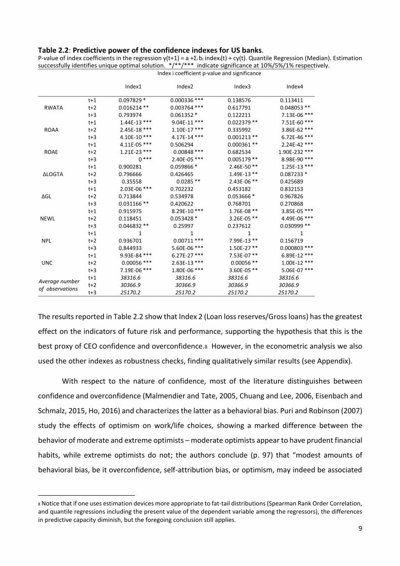
Table 2.2: Predictive power of the confidence indexes for US banks. P-value of index coefficients in the regression y(t+1) = a +Σi bi indexi(t) + cy(t). Quantile Regression (Median). Estimation successfully identifies unique optimal solution. */**/*** indicate significance at 10%/5%/1% respectively. Index i coefficient p-value and significance

Index1 Index2 Index3 Index4

RWATA t+1 0.097829 * 0.000336 *** 0.138576 0.113411 t+2 0.016214 ** 0.003764 *** 0.617791 0.048053 ** t+3 0.793974 0.061352 * 0.122211 7.13E-06 ***

ROAA t+1 1.44E-13 *** 9.04E-11 *** 0.022379 ** 7.51E-60 *** t+2 2.45E-18 *** 1.10E-17 *** 0.335992 3.86E-62 *** t+3 4.10E-10 *** 4.17E-14 *** 0.001213 ** 6.72E-46 ***

ROAE t+1 4.11E-05 *** 0.506294 0.000361 ** 2.24E-42 *** t+2 1.21E-23 *** 0.00848 *** 0.682534 1.90E-232 *** t+3 0 *** 2.40E-05 *** 0.005179 ** 8.98E-90 ***

∆LOGTA t+1 0.900281 0.059866 * 2.46E-50 ** 1.25E-13 *** t+2 0.796666 0.426465 1.49E-13 ** 0.087233 * t+3 0.35558 0.0285 ** 2.43E-06 ** 0.425689

∆GL t+1 2.03E-06 *** 0.702232 0.453182 0.832153 t+2 0.713844 0.534978 0.053666 * 0.967826 t+3 0.031166 ** 0.420622 0.768701 0.270868

NEWL t+1 0.915975 8.29E-10 *** 1.76E-08 ** 3.85E-05 *** t+2 0.118451 0.053428 * 3.26E-05 ** 4.49E-06 *** t+3 0.046832 ** 0.25997 0.237612 0.030999 **

NPL t+1 1 1 1 1 t+2 0.936701 0.00711 *** 7.99E-13 ** 0.156719 t+3 0.844933 5.60E-06 *** 1.50E-27 ** 0.000803 ***

UNC t+1 9.93E-84 *** 6.27E-27 *** 7.53E-07 ** 6.89E-12 *** t+2 0.00056 *** 2.63E-13 *** 0.00056 ** 1.00E-12 *** t+3 7.19E-06 *** 1.80E-06 *** 3.60E-05 ** 5.06E-07 ***

Average number of observations

t+1 38316.6 30366.9 25170.2

38316.6 30366.9 25170.2

38316.6 30366.9 25170.2

38316.6 30366.9 25170.2

t+2 t+3

The results reported in Table 2.2 show that Index 2 (Loan loss reserves/Gross loans) has the greatest

effect on the indicators of future risk and performance, supporting the hypothesis that this is the

best proxy of CEO confidence and overconfidence.8 However, in the econometric analysis we also

used the other indexes as robustness checks, finding qualitatively similar results (see Appendix).

With respect to the nature of confidence, most of the literature distinguishes between

confidence and overconfidence (Malmendier and Tate, 2005, Chuang and Lee, 2006, Eisenbach and

Schmalz, 2015, Ho, 2016) and characterizes the latter as a behavioral bias. Puri and Robinson (2007)

study the effects of optimism on work/life choices, showing a marked difference between the

behavior of moderate and extreme optimists – moderate optimists appear to have prudent financial

habits, while extreme optimists do not; the authors conclude (p. 97) that “modest amounts of

behavioral bias, be it overconfidence, self-attribution bias, or optimism, may indeed be associated

8 Notice that if one uses estimation devices more appropriate to fat-tail distributions (Spearman Rank Order Correlation, and quantile regressions including the present value of the dependent variable among the regressors), the differences in predictive capacity diminish, but the foregoing conclusion still applies.

10

with seemingly reasonable decision-making.” On the same theme, Goel and Thakor (2008)

distinguish three degrees of confidence: extravagant diffidence, moderate overconfidence, and

extravagant overconfidence. Extravagantly diffident CEOs reject high-profit projects, to the

detriment of the company’s value, while the extravagantly overconfident invest less in information

and so jeopardize stakeholders. Moderately overconfident CEOs are found to benefit shareholders

and increase the value of the firm.

Following Goel and Thakor, we too distinguish three levels of confidence: underconfidence,

mid-confidence and overconfidence, positing qualitative behavioral differences between the three

types of bank. In addition, we define as overconfident the banks in the bottom decile of the

distribution of Loan loss reserves/Gross loans (or Loan loss provisions/Gross loans), and as

underconfident those in the top decile. All the other banks are defined as mid-confident, i.e. having

an intermediate level of confidence.9

In fact, Figure 2.1 shows that banks’ confidence increased between 2001 and 2007 and dropped

sharply in 2008-2009. It was not restored until after 2011; the trend is more distinct when the proxy

is loan loss reserves (not provisions) over gross loans.

Figure 2.1. American banks’ confidence and over-confidence in the period 2001-2013

Confidence on the left-hand scale, overconfidence on the right. The confidence index is a weighted average of Loan loss

reserves/Gross loans and Loan loss provisions /Gross loans for all the banks and for the banks in the bottom decile of

the annual distribution of the corresponding indicator.

-1.50

-1.45

-1.40

-1.35

-1.30

-1.25

-1.20

-.48

-.44

-.40

-.36

-.32

-.28

2001

2002

2003

2004

2005

2006

2007

2008

2009

2010

2011

2012

2013

- LLR (all banks)

- LLR (overconfident banks)

-.4

-.3

-.2

-.1

.0

0

4

8

12

16

2001

2002

2003

2004

2005

2006

2007

2008

2009

2010

2011

2012

2013

- LLP (all banks)

- LLP (overconfident banks)

9 Puri and Robinson (2005) take the right-most 5% of CEOs in their proxy of optimism to be extreme optimists, while Ma

(2014) defines the top 10% of his confidence indicator as overconfident. However, as a robustness check, we also

considered the top and bottom 20% of the distribution of loan loss reserves/gross loans , finding similar results. See

Appendix.

11

Next we investigate the determinants of confidence for our three categories, including the

impact of current news and expectations on confidence, and responses to bad and good news.

3. The determinants of confidence and overconfidence in banking

Barberis (2013), Foote et al. (2012) and Gennaioli et al. (2015b) all emphasize that in a context

of bounded rationality decision-makers extrapolate past trends. Akerlof and Shiller (2009) note the

role of success stories in the formation of expectations, likening the transmission of confidence

between individuals to that of epidemic disease. We therefore expect good news on past

performance to fuel confidence and expectations of still better performance by all the banks. In a

boom, good news increases and non-performing loans decline, both factors favoring greater

confidence and optimism and further balance-sheet expansion.

Hypothesis 1. Banks’ confidence increases with good news and decreases with bad news.

In addition, we hypothesize that banks differ in their responses to good and bad news.

Hypothesis 2. Overconfident (underconfident) banks respond more (less) to good news and less

(more) to bad news than the other banks.

Overconfident CEOs are likely to overestimate the importance of good news and

underestimate bad, reflecting their overoptimistic view of the economy (Odean, 1998, Daniel et al.,

1998, Daniel and Hirshleifer, 2015); for underconfident banks, the inverse holds, given their

pessimism over the economy.

Therefore, we expect current news to have differential effects on different types of bank.

Good news will induce the overconfident to trim their loan loss reserves and provisions more

significantly, and they will increase their provisioning less in response to bad news. Pain (2003) and

Bikker and Metzemakers (2005) document that an increase in real GDP growth reduces banks’

provisions. Laeven and Majnoni (2003) and Black and Gallemore (2012) report that during a business

expansion banks tend to defer the accounting recognition of expected losses until adverse cyclical

conditions start to set in.

Beyond their response to current news, we also assume that CEOs differ in their expectations

for the future.

12

Hypothesis 3. Overconfident (underconfident) banks’ CEOs have an optimistically (pessimistically

) biased view of the future.

Gennaioli et al. (2015a) gives evidence that the actual investments of non-financial

corporations are driven by expectations, which are not rational. Moreover, Barberis and Thaler

(2003), among others, state that overconfident CEOs have more optimistic views of the future, while

Malmendier and Tate (2005) show that they overestimate the returns to their investment projects.

Ahmed et al. (1999) document that loan loss provisions are negatively correlated with changes in

expected earnings and with contemporaneous stock returns. We therefore assume that excessive

optimism or pessimism leads respectively to overestimation or underestimation of future returns.

Summarizing our hypothesis, we posit that the level of confidence is the result of good and

bad news today and expectations of good and bad news tomorrow. Good news and a better outlook

on the future increase confidence, but overconfident CEOs respond more strongly to good news

and less to bad. Consequently, we expect that the more confident banks will hold smaller loan loss

provisions and loan loss reserves relative to gross loans, owing to their rosier view of current news

and more optimistic vision of the future. For underconfident banks, the opposite holds.

Next, we evaluate the impact of current news on confidence and then assess how

expectations affect confidence for our three bank types.

To test the first two assumptions we estimated the following:

∆(LLR)*100= β0 + β1LLR(-1)*100+ β2∆LLR(-1) + β3UNC*100+ β4∆GL + β5∆NPL + β6NPL *100+ β7

LOGTA(-1)+ β8∆LOGTA+β9LOGTA+ β10IMPTE + β11TIER1+ β12OP+β13PBT+ β14 ∆PBT +β15GDP+

β16CLIF(-1)+ β17LOGSMK(-1) + β18∆LOGSMK + β19FEDFUND + ε (1)

in which ∆ denotes absolute variation, LOG denotes natural logarithm, (-1) indicates the previous

year, and ε is the error term. Table 4.1 gives the definitions of the variables. We distinguish between

internal and external determinants of confidence. Regressors from 1-14 are internal, regressors 15-

19 external. The former include balance-sheet determinants (non-performing loans, uncollectable

loans, profits, tier 1 regulatory capital and gross loans), while the latter comprise macroeconomic

indicators (real GDP growth, the value of current leading indicators, and the stock market index).

13

4. Data and methodology

We tested our hypotheses on a sample of American commercial, cooperative, and savings

banks.10 The data set includes the consolidated annual balance sheets of 10,223 banks in the United

States, or 84% of the American banks reported in the Bankscope database, provided by Bureau van

Dijk.11 We also used other data sources, such as Bondware, to compute loans net of securitization.

Table 4.1 shows the variables used in the econometric analysis and their sources.

Table 4.1 Variables and sources of the data

Definition Symbol Source

Bank-specific variables:

Size (log of total assets) LOGTA BankScope

Risk-weighted assets/Total assets RWATA BankScope

Risk Weighted Assets including floor/cap per Basel II RWAF BankScope

Leverage (Total assets / Total equity) Y_L1 BankScope

Loan loss provisions/Gross loans(-1) LLP BankScope

Loan loss reserves/Gross loans(-1) LLR BankScope

Non-performing Loans/Gross Loans NPL BankScope

Non-performing Loans/Total Equity NPLTE BankScope

Impaired loans/Gross loans IMP BankScope

Impaired Loans/Total Equity IMPTE BankScope

Uncollectable loans/Gross loans(-1). UNC BankScope

Liquid assets / Total assets LIQU BankScope

Deposits and short term funding/

Total assets DEP BankScope

Tier1 Regulatory capital ratio TIER1 BankScope

Operating profits / Total assets(-1) OP BankScope

Profits before taxes/Total assets PBT BankScope

Return on assets ROAA BankScope

10 We used only these categories of banks because of the substantial differences from other classes of banks reported in the Bankscope dataset (notably, bank holding & holding companies, finance companies, investment banks, real estate & mortgage banks, and specialized governmental credit institutions). 11 However, because observations for some banks were incomplete, our econometric analysis covers only 9,845 banks in the open sample and 5,838 banks in the closed sample.

14

Return on equity ROAE BankScope

Gross Loans GL BankScope

∆Gross Loans/Gross_Loans(-1)) ∆GL BankScope

Gross loans/Total assets(-1). GLTA BankScope

New loans/Gross loans(-1) NEWL BankScope

Net_interest_margin NIM BankScope

Total_long_term_funding /Total_liabilities LTF BankScope

Interbank_ratio IBR BankScope

(Operating profits +Loan Loss Provisions)/Total assets OPBT Bankscope, Bondware

Macro variables:

Three-month unsecured interbank rate – IRS

corresponding secured interest rate RISK3 Fed

Three-month unsecured interbank rate R3M Fed

Treasury bond Long term rate LTTB Fed

Official interest rates FED_FUND

Fed

Stock market index (log) (year 2000=100) LOGSMK Yahoo Finance

Composite leading indicator (end year) CLIF OECD

Real annual GDP growth GDP World Bank

Table 4.2 reports the summary statistics for the banks present in all the years considered.

Table 4.2 Summary statistics. American commercial, cooperative and savings banks. Period 2001-

2013. Closed sample.

All All Over Inter Under All All All All All

Obs. Mean Mean Mean Mean Max Min Std. Dev. Skew. Kurtosis

LLR 36884 1.33 0.376 1.221 3.155 32.2 0 0.923 7.349 135.665

100*LLP 36884 0.113 0.021 0.085 0.398 45.751 -23.077 0.719 12.214 634.955

∆(LLR) 36884 -0.007 -0.026 -0.024 0.111 17.75 -12.36 0.392 0.968 235.141

100*UNC 36884 -0.002 0.016 -0.024 0.096 66.4 -618.5 3.943 -132.434 19233.7

∆GL 36884 0.116 0.124 0.136 0.08 192 -0.976 1.36 96.425 12031.6

∆GL 36884 0.116 0.124 0.135 0.081 185.815 -0.966 1.327 94.633 11668.6

∆ (NPL) 36732 0.032 0.002 -0.014 -0.015 18.89 -24.05 0.787 2.394 91.096

NPL 36782 0.454 0.273 0.362 0.765 50.53 0 1.004 11.284 327.227

LOGTA 36884 4.399 4.764 4.456 3.937 13.221 1.099 1.049 0.954 6.43

∆ LOGTA 36884 0.07 0.06 0.083 0.035 4.995 -1.93 0.138 6.201 121.381

GLTA 36623 0.599 0.642 0.603 0.448 1.060 0.002 0.170 -0.433 2.831

IMPTE 36782 0.027 0.018 0.023 0.034 4.34 0 0.071 18.749 709.147

TIER1TIER1 36876 19.154 24.965 16.873 25.167 485.7 2.58 11.801 6.386 128.864

15

OP 36883 1.246 1.103 1.381 1.444 39.78 -23.4 1.076 4.818 200.252

OPBT 36883 1.325 1.117 1.442 1.716 42.053 -23.4 1.124 8.183 237.163

∆ (OPBT) 36879 0 -0.05 0.038 0 144.9 -14.871 1.053 71.616 9744.15

ROAA 36625 0.99 0.711 0,881 1.045 25.09 -21.69 0.886 2.269 117.74

ROAE 36625 9.1 6.378 8,963 7.711 181.71 -124.03 7.738 0.472 33.55

NIM 36625 3.99 3.279 4,119 4.392 70.58 0 1.264 11.786 380.18

100*LTF 36884 3.402 6.947 3.463 1.646 98.734 -6.8 6.418 3.111 17.328

100*DEP 36883 95.817 92.106 95.794 97.226 142.157 0 6.65 -3.092 18.307

100*LIQU 36884 10.834 9.363 9.491 13.462 86.885 0 9.244 2.227 10.142

IBR 1563 45.548 NA NA NA 962.75 0 128.131 3.924 19.836

RWAF 32758 176.704 220.821 216.451 245.88 455722 1 4166.13 84.164 8015.10

RWATA 32758 0.635 0.551 0.66 0.593 3.151 0.025 0.144 0.692 14.21

Y_L1 36623 9.709 9.299 10.143 8.417 65.5 1.037 2.891 0.692 9.748

GDP 36623 0.945 - - - 2.9 -3.6 1.542 -1.323 4.834

CLIF 36623 99.645 - - - 101.396 95.647 1.608 -0.965 3.202

LOGSMK 36623 7.076 - - - 7.41 6.855 0.146 0.235 2.531

100*∆ LOGSMK 36623 -0.013 - - - 0.176 -0.248 0.148 -0.262 1.403

FED_FUND 36623 2.377 - - - 5.05 0.125 1.741 0.219 1.659

R3M 36623 2.626 - - - 5.319 0.281 1.687 0.232 1.705

RISK3 36623 0.196 - - - 1.414 -0.025 0.386 2.315 7.312

RTREASURY 36623 4.11 - - - 5.021 1.803 0.835 -1.149 3.623

The closed sample counts some 36,800 observations. Of these, 9.79% refer to overconfident

banks and 9.95% to underconfident banks.

Banks at our three degrees of confidence differ in several aspects. Overconfident banks are

larger and have a greater propensity to lend (their lending is equal to 64% of total assets, compared

with 60% for mid-confidents and 45% for underconfidents). On average, however, during our period

it was mid-confident, not overconfident, banks that registered the sharpest increases in lending and

total assets. In addition, mid-confident banks are more highly leveraged, with the highest portfolio

risk and the lowest profits, but they also give the highest return on capital to investors.

Underconfident banks have a lower propensity to lend, with the highest non-performing loan and

loan loss ratios, but also the highest operating profits and interest rate margins. This suggests that

underconfident banks may be lending to riskier borrowers. For the period as a whole, the mid-

confident banks increased their ratio of loan loss reserves to gross loans, while the other banks

lowered it.

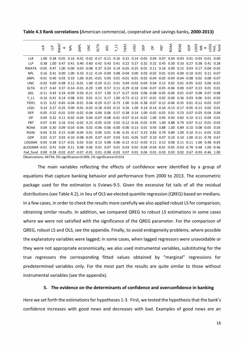
Finally, Table 4.3 reports the correlation matrix among the variables. We opted for rank

correlations instead of the traditional Pearson r correlation, in view of the high Kurtosis value of all

the balance-sheet data.

16

Table 4.3 Rank correlations (American commercial, cooperative and savings banks, 2000-2013)

LLR

LLP

RW

AT

A

NP

L

∆N

PL

UN

C

GLT

A

∆G

L

Y_L1

TIER

1

LIQ

U

DEP

OP

PB

T

RO

AA

RO

AE

GD

P

LOG

S

MK

∆

LOG

S

MK

Fe

d_

fun

d

LLR 1.00 0.38 -0.05 0.16 -0.01 -0.02 -0.17 -0.11 -0.16 0.15 0.14 -0.05 0.04 0.07 0.04 -0.03 0.01 -0.03 -0.01 0.00

LLP 0.38 1.00 0.47 0.41 0.40 0.60 0.42 0.43 0.41 0.22 0.27 0.32 0.32 0.45 0.30 0.33 0.27 0.38 0.41 0.28

RWATA -0.05 0.47 1.00 -0.00 0.03 -0.08 0.37 0.24 0.14 -0.65 -0.25 -0.01 0.11 0.16 0.09 0.15 0.03 0.17 0.04 -0.02

NPL 0.16 0.41 -0.00 1.00 0.33 0.12 -0.14 -0.09 0.08 -0.04 0.00 0.03 -0.02 0.01 -0.03 -0.00 -0.10 -0.01 0.11 -0.07

∆NPL -0.01 0.40 0.03 0.33 1.00 -0.01 -0.01 0.03 0.01 -0.01 -0.01 -0.02 -0.04 -0.02 -0.04 -0.04 -0.08 0.02 0.08 -0.07

UNC -0.02 0.60 -0.08 0.12 -0.01 1.00 -0.29 -0.21 0.01 0.04 -0.02 -0.04 0.04 0.15 0.02 0.01 -0.05 0.02 0.06 -0.01

GLTA -0.17 0.42 0.37 -0.14 -0.01 -0.29 1.00 0.57 0.11 -0.29 -0.18 0.04 -0.07 -0.05 -0.06 0.00 0.07 0.13 0.01 0.01

∆GL -0.11 0.43 0.24 -0.09 0.03 -0.21 0.57 1.00 0.17 -0.27 -0.03 0.06 -0.08 -0.05 -0.06 0.01 -0.07 0.08 0.07 -0.08

Y_L1 -0.16 0.41 0.14 0.08 0.01 0.01 0.11 0.17 1.00 -0.73 -0.12 0.57 -0.01 0.02 -0.00 0.36 0.03 0.06 0.01 -0.03

TIER1 0.15 0.22 -0.65 -0.04 -0.01 0.04 -0.29 -0.27 -0.73 1.00 0.26 -0.38 -0.07 -0.12 -0.06 -0.35 0.01 -0.12 -0.03 0.07

LIQU 0.14 0.27 -0.25 0.00 -0.01 -0.02 -0.18 -0.03 -0.12 0.26 1.00 0.14 -0.14 -0.16 -0.13 -0.17 -0.05 -0.12 0.02 0.01

DEP -0.05 0.32 -0.01 0.03 -0.02 -0.04 0.04 0.06 0.57 -0.38 0.14 1.00 -0.02 -0.02 0.01 0.23 0.07 -0.03 -0.04 0.04

OP 0.04 0.32 0.11 -0.02 -0.04 0.04 -0.07 -0.08 -0.01 -0.07 -0.14 -0.02 1.00 0.95 0.93 0.83 0.10 0.11 -0.04 0.01

PBT 0.07 0.45 0.16 0.01 -0.02 0.15 -0.05 -0.05 0.02 -0.12 -0.16 -0.02 0.95 1.00 0.88 0.79 0.07 0.12 -0.01 -0.03

ROAA 0.04 0.30 0.09 -0.03 -0.04 0.02 -0.06 -0.06 -0.00 -0.06 -0.13 0.01 0.93 0.88 1.00 0.89 0.10 0.08 -0.05 0.03

ROAE -0.03 0.33 0.15 -0.00 -0.04 0.01 0.00 0.01 0.36 -0.35 -0.17 0.23 0.83 0.79 0.89 1.00 0.10 0.11 -0.03 0.02

GDP 0.01 0.27 0.03 -0.10 -0.08 -0.05 0.07 -0.07 0.03 0.01 -0.05 0.07 0.10 0.07 0.10 0.10 1.00 -0.11 -0.78 0.67

LOGSMK -0.03 0.38 0.17 -0.01 0.02 0.02 0.13 0.08 0.06 -0.12 -0.12 -0.03 0.11 0.12 0.08 0.11 -0.11 1.00 0.48 -0.03

∆LOGSMK -0.01 0.41 0.04 0.11 0.08 0.06 0.01 0.07 0.01 -0.03 0.02 -0.04 -0.04 -0.01 -0.05 -0.03 -0.78 0.48 1.00 -0.46

Fed_fund 0.00 0.28 -0.02 -0.07 -0.07 -0.01 0.01 -0.08 -0.03 0.07 0.01 0.04 0.01 -0.03 0.03 0.02 0.67 -0.03 -0.46 1.00

Observations: 44734; 5% significance=0.009; 1% significance=0.014

The main variables reflecting the effects of confidence were identified by a group of

equations that capture banking behavior and performance from 2000 to 2013. The econometric

package used for the estimation is Eviews-9.5. Given the excessive fat tails of all the residual

distributions (see Table 4.2), in lieu of OLS we elected quantile regression (QREG) based on medians.

In a few cases, in order to check the results more carefully we also applied robust LS for comparison,

obtaining similar results. In addition, we compared QREG to robust LS estimations in some cases

where we were not satisfied with the significance of the QREG parameter. For the comparison of

QREG, robust LS and OLS, see the appendix. Finally, to avoid endogeneity problems, where possible

the explanatory variables were lagged; in some cases, when lagged regressors were unavoidable or

they were not appropriate economically, we also used instrumental variables, substituting for the

true regressors the corresponding fitted values obtained by “marginal” regressions for

predetermined variables only. For the most part the results are quite similar to those without

instrumental variables (see the appendix).

5. The evidence on the determinants of confidence and overconfidence in banking

Here we set forth the estimations for hypotheses 1-3. First, we tested the hypothesis that the bank’s

confidence increases with good news and decreases with bad. Examples of good news are an

17

increase in profits and a reduction in non-performing loans, or an increase in real GDP and a rise in

the stock market index.

Table 5.1 Estimation of the determinants of confidence

Years: 2001-2013. Method: Quantile Regression (Median), Huber Sandwich Standard Errors & Covariance, Sparsity method: Kernel (Epanechnikov) using residuals, Bandwidth method: Hall-Sheather, bw=0.020706, Estimation successfully identifies unique optimal solution; Δ() indicate change; */**/*** indicate significance at 10/5/1% of probability respectively. Notice that a higher value of the dependent variable corresponds to a lower level of confidence. Hence (apart from the lagged dependent variable) a negative coefficient corresponds to an increase in confidence.

Dependent Variable: ∆(LLR) ∆(LLR) LLR LLR ∆(LLR) ∆(LLR) Type of sample Open close open close open close

Fixed effects No no yes yes yes yes Estimation Method QREG QREG QREG with IV QREG with IV QREG with IV QREG with IV

Regressors / Equations (1) (2) (3) (4) (5) (6)

C -0.03422 -0.01783 -0.01937*** -0.01869*** -0.00973*** -0.00930*** LLR(-1) -0.06440*** -0.05824*** 0.47074*** 0.55502*** -0.35972*** -0.21639***

∆ (LLR(-1)) -0.00135 0.00255** -0.07631* -0.11297** 0.14529*** 0.09141*** 100* UNC -0.06270*** -0.27417** -0.06411*** -0.09217*** -0.23681*** -0.30414***

∆ GL -0.08140*** -0.50676*** -0.15280*** -0.25381*** -0.34077*** -0.50310*** ∆ (NPL) 0.04208*** 0.01561** 0.06239*** 0.04438*** 0.03943*** -0.00189 NPL(-1) 0.01078*** -0.00176 0.06385*** 0.03816*** 0.04326*** -0.00066

LOGTA (-1) 0.00080 0.00592*** 0.02525** -0.00701 0.04828*** 0.04978*** ∆ LOGTA -0.01299 0.15891 -0.06225** 0.02454 0.01372 0.06134***

LOG(GLTA (-1))) 0.00469 -0.01244*** -0.11555 -0.20173*** 0.12889*** 0.09943*** IMP 0.10057*** 0.38963*** 0.02261*** 0.21870* 0.13464*** 0.66834***

TIER1 -0.00014*** -0.00034** 0.00642*** 0.00462*** 0.00460*** 0.00264*** OP(-1) -0.08332*** -0.20593** -0.20289*** -0.20645*** -0.05026 -0.08698***

PBT 0.08670*** 0.21230** 0.20099*** 0.20958*** 0.04365 0.08756*** ∆(PBT) -0.06781*** -0.17999 -0.18533*** -0.18462*** -0.03089 -0.06830**

GDP -0.00343*** -0.00098 0.01215*** 0.00825*** 0.00307** 0.00172 CLIF 0.00117 0.00072 0.00369** 0.00313 0.00142 0.00052

LOG(SMK(-1)) -0.00065 -0.00253 -0.04056* -0.03337 -0.04580 -0.03312*** ∆LOG(SMK) -0.06763*** -0.05759*** -0.18914*** -0.14143*** -0.08588*** -0.06180*** Fed_fund -0.00644*** -0.00384*** -0.00417*** -0.00313* -0.00435*** -0.00374***

No. observations: 50,461 36,454 28,674 22,898 28,674 22,898

Adj, Pseudo R-squared 0.04556 0.10897 0.06761 0.06797 0.09968 0.12301

In the QREG estimations with Instrumental Variables (IV), the latter are applied to the lagged variables in the case of fixed effects.

Employing IV, the parameter values change when we estimate both the level and the variation of the dependent variables.

This is confirmed by the results shown in the table. An increase in non-performing loans reduces

confidence, while an increase in profitability, GDP, current leading indicators and stock market

performance increase the confidence of all banks. In addition, a rise in the fed funds rate has a

positive impact on confidence, as banks’ profits are higher (see Table 4.3), since among other things

their interest rate margins widen. The results do not vary greatly between the open and the closed

sample, or for the most part between estimates with and without instrumental variables

estimations.

18

Finally, we again estimated equation (1), this time with the fixed effect model, to check whether the

results may not depend on bank idiosyncratic factors.12 In general the results (columns 5 and 6 in

Table 5.1) are not very different from the quantile regression estimations without fixed effects

(columns 1 and 2).

Table 5.1 shows that almost all the internal and external determinants of confidence are significant.

To determine which are more relevant, we ran estimations of the relevance of the regressors. The

results are given in Table 5.2, which after the value of the coefficient also shows (in brackets) the

importance of the regressors, 1 indicating the most relevant.

In the short run, the most important determinant is profitability, followed by uncollectable

loans/gross loans and non-performing loans/gross loans. Past profits increase confidence, non-

performing loans reduce it. On the other hand, current gross profits increase reserves, suggesting

that banks may use the latter, among other things, to smooth income. Interestingly, an increase in

gross loans (net of securitized loans) has a positive impact on confidence, and so does larger bank

size. This suggests that when banks expand loans they are strongly confident of their profitability.

The lagged dependent variable is also relevant, suggesting that confidence is highly persistent.

Overall, the external determinants of confidence are less relevant than the internal. The most

important external factors are stock market performance and the federal funds rate. As we

expected, an increase in both of these variables has a positive effect on confidence. That is, the

empirical evidence supports hypothesis 1.

12 Since the quantile regression does not compute the fixed effects, we calculated them by de-meaning the value of each regressor for each bank. And for the open sample we deleted all the banks with fewer than five observations (3% of the total).

19

Table 5.2 Estimation of the determinants of confidence: Relevance of the regressors Years: 2001-2013. Method: Quantile Regression (Median), Huber Sandwich Standard Errors & Covariance, Sparsity method: Kernel (Epanechnikov) using residuals, Bandwidth method: Hall-Sheather, bw=0.020706, Estimation successfully identifies unique optimal solution. Notice that a higher value of the dependent variable corresponds to a lower level of confidence. Hence, (apart from the lagged dependent variable) a negative coefficient corresponds to an increase in confidence. Dependent Variable: ∆(LLR) ∆(LLR) ∆(LLR) ∆(LLR) LLR LLR

Type of sample open closed open Same sample of column(3) without risk

open closed

Fixed effects no no no no yes yes

Estimation Method qreg qreg qreg qreg qreg

with IV qreg

with IV Regressors / equations (1) (2) (3) (4) (5) (6)

LLR(-1) -3.671(3) -3.320(6) -3.528(6) -3.528(6) -3.156(4) -2.653(4) ∆ (LLR(-1)) -0.047(17) 0.089(15) 0.038(18) 0.038(17) -0.396(15) -0.586(12) 100* UNC (-1) -1.602(5) -7.005(3) -10.144(3) -10.144(3) -1.606(6) -2.309(5) ∆ GL -0.581(9) -3.620(5) -4.758(5) -4.758(5) -0.971(11) -1.614(7) ∆ (NPL) 0.800(7) 0.297(12) 0.488(9) 0.488(8) 1.092(9) 0.777(11) NPL(-1) 0.280(10) -0.046(18) 0.381(11) 0.381(10) 1.657(5) 0.990(10) LOGTA (-1) 0.047(18) 0.348(11) 0.301(12) 0.301(11) 0.211(17) -0.059(19) ∆ LOGTA -0.061(16) 0.742(7) 0.680(7) 0.680(7) -0.284(16) 0.112(18) LOG(GLTA (-1))) 0.141(12) -0.374(10) -0.404(10) -0.404(9) -1.027(10) -1.793(6) IMP 0.074(15) 0.287(13) -0.120(17) -0.120(16) 0.016(19) 0.151(17) TIER1 -0.107(14) -0.249(14) 0.011(19) 0.011(18) 1.456(7) 1.048(8) OP(-1) -4.999(2) -12.356(2) -13.861(2) -13.861(2) -5.876(2) -5.979(2) PBT 5.202(1) 12.738(1) 15.085(1) 15.085(1) 5.930(1) 6.184(1) ∆(PBT) -1.695(4) -4.500(4) -7.660(4) -7.660(4) -4.753(3) -4.734(3) GDP -0.241(11) -0.069(17) -0.147(16) -0.147(15) 0.860(12) 0.584(13) CLIF 0.140(13) 0.086(16) -0.005(20) -0.005(19) 0.191(18) 0.162(16) LOG(SMK(-1)) -0.009(19) -0.035(19) -0.202(15) -0.202(14) -0.530(13) -0.436(14) ∆LOG(SMK) -0.644(8) -0.549(9) -0.292(14) -0.292(13) -1.338(8) -1.001(9) Fed_fund -0.997(6) -0.595(8) -0.295(13) -0.295(12) -0.415(14) -0.312(15) RWATA(-1) - - 0.661(8) - - -

The relevance is estimated by multiplying every absolute coefficient value by the median absolute deviation (MAD) of its

corresponding regressor. QREG with IV = IV are applied to the lagged variables in the case of fixed effects. In equation (3) the variable

risk_weighted_assets(-1) is also included among the regressors. Parameters are multiplied by 100.

As a robustness check, we divided the sample period into pre- and post-2007. Since up to 2007 good

news predominated and bad news afterwards, banks should respond in the two sub-periods

similarly to the way they respond to good and to bad news respectively. And the results confirm

this prediction. Banks’ confidence rose before 2007 and declined thereafter. In any case, for all the

categories of bank the effect of news on confidence was greater after 2007 than before.13

Notice that the lagged dependent variable in the foregoing regressions may produce biased

estimations if the residuals are autocorrelated. We accordingly checked for autocorrelation, which

in most cases is not significant, save where the dependent variable is the level of confidence and

13 Specifically, the econometric analysis on fitted values shows that after 2007 overconfident banks reduced their confidence in response to bad news, but they also became systematically less confident, shifting the entire relationship between confidence and their determinants downward. By contrast, underconfident banks became systematically more confident after the crisis. These results hold for both the open and the closed sample. To save on space we do not report them, but they are available from the authors upon request.

20

fixed effects estimation is employed (see Table 5.3). However, when fixed effects were considered,

we always used instruments for the lagged dependent variable, as in that case coefficients are

always biased if the number of banks is large and the number of observations is small. And even

then the problem of bias owing to autocorrelation of residuals should not be serious.

TABLE 5.3: Residuals autocorrelation (QREG estimation). Years: 2001-2013 Method: Quantile Regression (Median), Huber Sandwich Standard Errors & Covariance, Sparsity method: Kernel (Epanechnikov) using residuals, Bandwidth method: Hall-Sheather, bw=0.020706, Estimation successfully identifies unique optimal solution.

Residuals

from

Equation 1 in

Column

1 Tab.5.1 2 Tab 5.1 3 Tab. 5.1 4 Tab. 5.1 5 Tab. 5.1 6 Tab. 5.1

Sample open closed open closed open closed

Fixed effects no no

Yes (with IV for

the lagged

dependent

variable)

Yes (with IV for

the lagged

dependent

variable)

Yes (with IV for

the lagged

dependent

variable)

Yes (with IV for

the lagged

dependent

variable)

Dependent

variable ∆(LLR) ∆(LLR) LLR LLR ∆(LLR) ∆(LLR)

Without

constant 0.01179 (0.1892)

-0.00630 (0.5824)

0.708080 (0.0000)

0.73508 (0.0000)

-0.01497 (0.4014)

-0.00700 (0.7256)

With

constant 0.01147 (0.1928)

0.00655 (0.5575)

0.70808 (0.0000)

0.73452 (0.0000)

-0.01520 (0.3932)

-0.00790 (0.7077)

Numbers in brackets are the probability level.

Next, we checked for heteroscedasticity, finding that the absolute value of the residuals is positively

correlated with confidence. So we tested whether the relationship between confidence and

residuals is the same for our three confidence levels. The results are reported in Table 5.4: the

dummies for overconfidence and underconfidence are both significant, indicating that extreme

degrees of confidence have a positive effect on the absolute value of the residuals.

Since the Ramsey test on the equations of Table 5.1 suggests non-linearity, we controlled for it in

the relationship between confidence and its determinants. In particular, we considered whether the

determinants of confidence differ with the bank’s degree of confidence,14 by applying dummy

variables to the parameters of the different categories.15

14 To select overconfident (underconfident) banks, we cut the observations off at the bottom and top 10% for the ratio of loan loss reserves to gross loans. Then for each year we defined as overconfident or underconfident the banks that in that year had a value of the confidence index below or above this threshold value. 15 In estimating the separate effect of the three types of bank we considered the problem that overconfident or underconfident banks may be so classed in part because their residuals are particularly low or high, but this creates a correlation between residuals and the dummy used to define the group, resulting in biased estimates. In order to avoid this, we applied instruments to the dummies defining the types. We estimated the dummies by considering the fitted values of loan loss reserves given in Table 5.1. Then for each type we used a probit to estimate the probability of the

21

Table 5.4: Analysis of residual volatility Dependent variable: absolute value of the residuals from the equation estimated in Table 5.1. Estimation method: Quantile regression.

Open sample Open sample Closed Open sample Closed sample

Fixed effects No no no yes yes

eq (1) (2) (3) (4) (5)

Residuals from Eq.1 Table 5.1 Eq.1 Table 5.1 Eq.2 Table 5.1 Eq.3 Table 5.1 Eq.4 Table 5.1

CONST -0.016350*** -0.01090*** 0.00166 -0.03158*** -0.02197***

Abs(resid) at t-1 0.152691*** 0.15733*** 0.01890 -0.06178*** -0.05476***

E[LLR/GL] 0.071738*** - 0.05233*** 0.12109*** 0.11322***

LLR(t-1)/GL(-1) - 0.06772*** - -

Overconfidence IV dummy 0.036549*** - 0.02844*** 0.06481*** 0.05715***

Underconfidence IV dummy 0.052143*** - 0.10253*** 0.11908*** 0.10848***

Overconfidence dummy at t-1 - 0.02877*** - -

Underconfidence dummy at t-1 - 0.02879*** - -

Obs 38,454 38,454 28,769 23,667 19,141

Adj Pseudo R-squared 0.09645 0.09458 0.06295 0.09926 0.09542

The overall impact of the determinants of confidence is similar to that reported in Table 5.1, but in

Table 5.5 the determinants differ between bank types . First, overconfident CEOs have greater

persistence of confidence than others. Second, mid-confident CEOs respond more strongly to news

than overconfident CEOs, and sometimes in the opposite direction. Specifically, mid-confident CEOs

react more forcefully to news of profits and losses and to changes in the stock market.

Interestingly, regardless of the CEO’s level of confidence, it never reacts to indicators of real

economic performance (see Table 5.5).16 Moreover, using the methodology of Engle and Hendry

(1993), we estimated whether the differences between confidence classes are temporary or

persistent, finding qualitatively similar results in the long run as well.17

bank belonging to a given group in relation to this fitted value and the dummy for confidence taken at t-1.The results are available from the authors upon request. 16 The qualitative results hold for the closed sample as well. To save on space, we do not report these results, but they are available from the authors upon request.

17We performed the econometric analysis also using the fixed effect model, again obtaining results similar to those in

Table 5.5. They are available from the authors upon request.

22

Table 5.5: Estimation of the determinants of confidence with dummy variables by category of bank Years: 2001-2013. Method: Quantile Regression (Median), Huber Sandwich Standard Errors & Covariance, Sparsity

method: Kernel (Epanechnikov) using residuals, Bandwidth method: Hall-Sheather, bw=0.020706, IV applied to

dummies for over- and under-confident banks. Estimation successfully identifies unique optimal solution; D() indicate

change; */**/*** refer to the coefficient significance at 10%/5%/1% level respectively; and °/°°/°°° refer to the

significance of the difference between coefficients of overconfidents and underconfidents with respect to mid-confident

banks. Notice that a higher value of the dependent variable corresponds to a lower level of confidence. Hence (apart

from the lagged dependent variable) a negative coefficient of LLR and D(LLR) corresponds to an increase in confidence.

Dependent Variable: ∆(LLR) Type of sample open

Fixed effects no Estimation Method QREG

mid-confident overconfident underconfident

Constant -0.00071 -0.26610/ -0.22178/

LLR(-1) -0.07471*** 0.02013***/°°° -0.05617***/°

∆ (LLR(-1)) 0.00887 -0.00499/ -0.00054/

100* UNC -0.33037*** 0.02238***/°°° -0.52971***/°°°

∆ GL -0.49889*** 0.00518**/°°° -1.99297***/°°°

∆ (NPL) 0.01294*** 0.01717**/ 0.03432/

NPL(-1) -0.00354 0.00115/ 0.00266/

LOGTA (-1) 0.00923*** -0.00209**/°°° 0.02259***/°

∆ LOGTA 0.14921*** 0.02226/°°° 0.08731/

LOG(GLTA (-1))) -0.00172 -0.00097/ -0.00184/

IMP 0.53156*** 0.43058***/ 0.12698***/°°°

TIER1 0.00023** -0.00003**/°° 0.00219*/

OP(-1) -0.25218*** 0.00042/°°° -0.42398***/°°

PBT 0.25585*** -0.00194/°°° 0.45988***/°°

∆(PBT) -0.22015*** -0.00218/°°° -0.43521***/°°

GDP -0.00150 -0.00305/ -0.00335/

CLIF 0.00078 0.00263/ -0.00298/

LOG(SMK(-1)) -0.00521 0.00304/ 0.06746/

∆LOG(SMK) -0.06594*** -0.03202**/° 0.05317/

Fed_fund -0.00323*** -0.00438***/ -0.00553/

Obs. 45,999 Adj Pseudo R-squared 0.15674

This evidence supports the finding of previous work that overconfident CEOs are more

strongly affected by conservative bias, which leads investors to underweight new information

relative to priors (see Daniel et al., 1998).

Having established that overconfident CEOs react less than others to news, we investigated

whether CEOs differ in the reaction to good and bad news. Following the literature, our Hypothesis

2 is that overconfident CEOs react more strongly than other CEOs to good news and less strongly to

bad, while the reverse holds for underconfident CEOs.

23

Table 5.6. CEOs’ reactions to good and bad news

Dependent variable: ∆ (LLR); Estimation Method: Quantile Regression (Median) with IV applied to the bank dummy classification (over, mid- and under-confidence). Estimation successfully identifies unique optimal solution. */**/*** indicate significance at 10/5/1% level. After slash °/°°/°°° indicate significance at 10/5/1% of probability of different coefficients between good and bad news.

Mid-confident Overconfident Underconfident

∆ (NPL) >0 Bad news 0.01559** 0.02361** 0.02798

0 Good news 0.00472 -0.01004 0.04447** / /°° /

PBT <1% Bad news 0.22914*** 0.00538 0.40483*** 1% Good news 0.24115*** 0.00894 0.46347*** /°°° / /°°°

∆(PBT) <0 Bad news -0.23726*** -0.02094 -0.41496***

0 Good news -0.16939*** 0.00440 -0.44168*** /°°° /°°° /

GDP <1% Bad news -0.00062 0.00049 -0.00868

1% Good news -0.00192 -0.00456** -0.00766 / /°° /

CLIF <100 Bad news 0.00190 0.00413** -0.00793 100 Good news 0.00184 0.00412** -0.00816 / / /

∆LOG(SMK) <0 Bad news -0.05447* -0.04585 0.30788

0 Good news -0.05601*** -0.02116 -0.02293 / / /

Obs 45,999

Adj Pseudo R2 0.16046 IV

Examples of good news are increases in profitability, real GDP, the stock market index and CLIF, as

well as a decline in Non-performing loans/total loans. Bad news consists in declines in the above

variables.

In Table 5.6 we report the estimates for banks’ reaction to good and bad news, which yield some

surprising results. Overconfident CEOs react more sharply to bad than to good news concerning ∆

(NPL), while the reverse holds for an increase in GDP. By contrast, mid-confident CEOs react more

strongly to good news on profitability and to better stock market performance. Thus the results

given in Table 5.6 provide only weak support for the thesis that overconfident banks, by comparison

with other banks, react more to good news and less to bad news. But the result does constitute

evidence that overconfident CEOs react less strongly to news, due to the greater persistency of their

beliefs. Indeed, our results bolster the thesis that this feature of overconfident behavior is more

important than the overreaction to good news and underreaction to bad that the literature

describes (Daniel et al., 1998).18

18 Additional support comes from the evidence that overconfident CEOs react less to internal than to external news. Internal news relates more closely to their own behavior, external news to that of others.

24

Table 5.4 shows that both overconfident and underconfident banks have a higher absolute value of

the residuals than the other banks. However, the residuals in the estimation of equation (1) may

reflect idiosyncratic factors, such as the quality of the management, irrational behavior, or other

determinants of confidence not included among our regressors, such as expectations about the

future. Accordingly we posit that the higher the absolute value of the residuals are, the more

relevant are expectations to the CEOs’ degree of confidence. To test this hypothesis, we performed

the following exercise. Using the fitted values of the dependent variable from the equation

estimated in Table 5.1, we computed the value of the residuals for the three confidence levels. It is

worth noting, as a preliminary, that if all three types attribute the same relevance to the future, the

absolute values of the residuals will not differ. The results, plotted in Figure 5.1, are surprising

indeed: other things being equal, the underconfident banks have a lower absolute value of the

residuals than the other banks practically throughout the period. Assuming that the residuals reflect

expectations about the future, this indicates that these banks have a systematically more optimistic

view of the future than the other banks.

Figure 5.1. Residuals of LLR/GL by category of bank (2001-2013) We used instrumental variables to correct for simultaneity bias between residuals and fitted values.

By contrast, the expectations of overconfident banks are more similar to those of the mid-

confident, albeit slightly more optimistic than the latter before the crisis and more pessimistic

25

afterwards. These results do not corroborate our hypothesis that more confident CEOs are more

optimistic about the future, but they do indicate that overconfident CEOs change their expectations

more than mid-confident CEOs (see Figure 5.1).19

Summing up the foregoing findings, confidence is the product of current news and expectations

about the future. Overconfident CEOs are more persistent in their beliefs and react less to current

news, while the contrary applies to mid-confident and underconfident CEOs. Finally, the

overconfident CEOs do not have an optimistically biased view of the future, but they change their

expectations more significantly than do mid-confident CEOs.

6. The effects of confidence on banking behavior and performance: the hypothesis

Above, we studied the determinants of confidence for our three types of bank. Now we address the

effects of confidence on banking behavior and performance, in both the short and the long run.

Delis et al. (2014), for US banks, and Demirguc-Kunt and Huizinga (2010), for a large sample of

international banks, find that risk was fairly stable up to 2001 and rose sharply between then and

2007. IMF (2014) also offers evidence that excessive risk-taking contributed to the global financial

crisis.

One strand of the literature has established that bank CEOs’ overconfidence played an

important role in increasing bank lending and leverage and weakening lending standards (Ho et al.,

2016; Ma, 2014; Sironi and Suntheim, 2012; Niu, 2010). Implicit in this literature is the assumption

that the financial crisis stemmed from the irrational conduct of bank managers and other economic

agents.

By contrast, for Geanokoplos (2010) and Danielsson and Shin (2009) rational behavior

implies that good news will build up confidence among all economic agents and lead banks to be

more prone to take risk and to expand their balance sheet. In this view, an increase in risk-taking is

not the product of behavioral bias but of greater confidence fueled by good economic performance.

On the other hand, Minsky (1992) and Shleifer and Vishny (2010) have shown that financial

intermediaries operating in markets influenced by investor sentiment have a cyclical behavior of

credit and investment and are unstable.

19 The values of the residuals in Figure 5.1 are obtained assuming that the values of the coefficients are equal for the three categories of banks; the results in Table 5.3 show that the coefficients are lower for overconfident banks, which may explain the corresponding residuals in Figure 5.1.

26

financial intermediaries operating in markets influenced by investor sentiment. Surprisingly,

the literature offers scanty evidence on the determinants of banks’ risk-taking before 2007.

Following this last approach, we assume that increases in confidence among all economic

agents spurred risk-taking, lending growth, and an increase in leverage.

Hypothesis 4: More confident bank managers take more risk.

This hypothesis rests on the assumption that more confident CEOs will tend to have better

expectations for future macroeconomic conditions and the opportunity for profit, and will expand

their banks’ business more forcefully. In addition, more confident CEOs take on more risk because

they feel better equipped to manage it. Takor (2014) examines a model in which thanks to sustained

banking profitability, all agents—banks, their fund suppliers and regulators—end up in an

“availability cascade” in which they overestimate the ability of bankers to manage risks and become

more tolerant of banks’ risk-taking, and banks invest in riskier and riskier assets. Goel and Thakor

(2008) and Eisenbach and Schmalz (2015) argue that overconfident managers underestimate risk

and so undertake actions entailing excessive risk. Figure 6.1 provides evidence for this hypothesis,

plotting the relationship between confidence and change in risk for the banks of our sample.

Figure 6.1 Loan loss reserves/Gross loans (LLR) and expected change in portfolio risk three years ahead

The horizontal axis shows the ratio of loan loss reserves to gross loans (LLR); the vertical axis, the

expected change in Risk-weighted/Total assets three years ahead. The data show an inverse

27

correlation between the two variables, suggesting that more confident banks (those with lower LLR)

increase their portfolio risk more substantially in the subsequent period.

Hypothesis 5. More confident banks lend more.

More confident banks are more optimistic that borrowers will be able to repay and are therefore

more willing to lend (see, e.g., Malmendier and Tate, 2005; Goel and Thakor, 2008; Campbell et al.,

2011; Ben-David et al., 2013). What is more, overconfident banks underestimate risk and so are

more likely to lend more and to grant credit to high-risk borrowers (Hirshleifer and Luo, 2001). Both

these effects lead the more confident banks to lend more and to loosen lending standards (Ma,

2014, Eisenbach and Schmalz, 2015).

Figure 6.2 Annual percentage growth in loans and leverage for confident and overconfident

American banks

(a) Percentage variation in Gross loans (b) Percentage variation in Leverage

0

4

8

12

16

20

24

2001

2002

2003

2004

2005

2006

2007

2008

2009

2010

2011

2012

2013

all banks

overconfident banks

-.3

-.2

-.1

.0

.1

.2

.3

.4

.5

.6

2001

2002

2003

2004

2005

2006

2007

2008

2009

2010

2011

2012

2013

all banks

overconfident banks

Figure 6.2 shows that both lending and leverage rose until 2009 and declined thereafter. But in both

cases the downturn was sharper at the overconfident banks. Moreover, the trends in lending and

leverage show some connection with the trend in confidence before and after the 2007 financial

crash (see Figure 2.1).

Hypothesis 6: More confident banks are more indebted.

28

Other things being equal, more confident banks expand their balance sheets more and are

consequently more likely to face capital constraints and resort to external funding.

Geanakoplos (2010) sets out a theoretical model to explain endogenous increases in optimism and

pessimism and how they affect leverage; Adrian and Shin (2010), and Malmendier et al. (2011) find

that banks prefer debt to equity when there are good opportunities for growth during a credit

boom. Beltratti and Stulz (2012) and Fahlenbrach et al. (2012) show that the preceding rise in

leverage played an important role in the ensuing financial crisis.20

Hypothesis 7: More confident banks fund their activities with a higher proportion of short-term debt.

More confident banks overvalue their ability to cope with adverse conditions, with high self-

attributions of the capacity to handle liquidity and market crises. So they are less worried about the

risk of funding long-term assets with short-term liabilities. Demirguc-Kunt and Huizinga (2010)

document that before 2007-2008 a sizable proportion of banks relied largely on short-term non-

deposit funding and on non-interest income.21

Hypothesis 8. More confident and riskier banks perform better in cyclical upswings and make larger

losses in downturns.

In favorable market conditions, banking confidence grows, spurring risk-taking and business

expansion. Consequently, in upswings the more confident banks are likely to make greater profits.

It follows that when the cycle turns downward, the banks whose assets were higher-risk are likely

to suffer more severe losses. This is the case for at least two reasons. First, in a crisis the riskier and

more highly indebted banks face worse conditions for refunding. And second, they are likely to

suffer larger losses as their borrowers presumably default more frequently.

Some researchers have investigated the effects of managerial overconfidence on the performance

of firms, showing that overconfident CEOs reduce firm value by overinvesting (see, e.g., Goel and

Thakor, 2008; Malmendier and Tate, 2008; Campbell et al., 2011). Fahlenbrach et al. (2012) find that

some bank characteristics connoting risk-taking are significantly correlated with poor performance

20 However, Geanakoplos (2010) points out that while the leverage cycle is not new, some new elements made the leverage cycle crisis of 2007-09 worse than its predecessors. First, leverage reached unprecedented levels. Second, this leverage cycle was actually double – both in securities on the repo market and on homes in the mortgage market – and the two cycles fed off one another. Third, CDSs, which were absent in previous cycles, enabled pessimists to leverage and thus made the crash much more precipitous than it would otherwise have been. 21 Palumbo and Parker (2009) and Fahlenbrach et al. (2012) show that the banks that expanded their activities more significantly before the 1998 crisis relied more heavily on short-term funding.

29

in both the 1998 and the 2007-08 crises. Laeven (2011) shows that after the global financial crisis

started in the summer of 2007 many US banks suffered deposit runs, fire sales, declining asset

values, and greater risk of being unable to meet their obligations. Finally, Beltratti and Stultz (2012)

and Ho et. al. (2016) provide evidence that during and after 2007-2008 the better-performing banks

were less highly leveraged, and that in the immediate run-up to the crisis they realized lower

returns. Thus there is evidence that the performance of banks during the crisis may be explained by

pre-crisis risk-taking.

Figure 6.3 provides evidence that the most heavily indebted American banks in 2007 also

had also the worst performance in 2008-2010.

Figure 6.3 American banks’ leverage in 2007 and ROA in 2008-2010 (Average values by decile).

In the sections that follow we check the foregoing hypothesis empirically. Specifically, we examine

the contributions of underconfident, mid-confident and overconfident banks to the increase in risk,

lending and leveraging in the run-up to the crisis and their effects on performance before and after

the 2007-2008 financial crash.

7. The effects of confidence on banks’ behavior and performance

7.1 Portfolio risk

Our measure of portfolio risk is the ratio of risk-weighted assets to total assets, weighting

the risk of each single asset with its importance in the total portfolio. Table 7.1 reports level of

.2

.3

.4

.5

.6

.7

2 4 6 8 10 12 14 16

leverage in 2007

RO

A (

mea

n va

lue

2008

-201

0)

30

portfolio risk and changes in it for the three types of bank before, during and after the 2008-2009

financial crash.

Table 7.1 Level and average yearly change in portfolio risk by type of bank.

Years Mid-confident Overconfident Underconfident All banks 2002-2007 Level Change Level Change Level Change Level Change

Mean 0.696066 0.005921 0.612748 0.009319 0.627328 0.000947 0.682488 0.008638 Median 0.703364 0.007692 0.609358 0.006933 0.617450 0.000000 0.692308 0.007557 Observations 40379 40355 3226 3212 3114 3111 49082 48812

2008-2009 Mid-confident Overconfident Underconfident All banks All banks Level Change Level Change Level Change Level Change

Mean 0.711739 -0.014377 0.626371 -0.002438 0.670883 -0.022999 0.697704 -0.011229 Median 0.724138 -0.010155 0.629518 -0.001110 0.684658 -0.014022 0.715148 -0.008888 Observations 12730 12363 1541 1205 982 953 16766 15218

20010-2013 Mid-confident Overconfident Underconfident All banks Level Change Level Change Level Change Level Change

Mean 0.649970 -0.013543 0.567893 -0.003028 0.648673 -0.019234 0.642918 -0.012277 Median 0.658251 -0.009468 0.562731 -0.004517 0.659440 -0.015145 0.655556 -0.009403 Observations 26992 26989 2310 2310 5928 5928 39413 39336

Surprisingly, it was mid-confident banks that had the greatest portfolio risk before, during

and after the crisis; and before 2008 they increased their risk more than the other banks. The

underconfident banks reduced portfolio risk most sharply during and after the crisis.22

To analyze the effects of confidence on banking behavior and performance, we consider separately

the impact of the explained level and/or variation of loan loss reserves (E[LRR] (or E[ΔLRR]), i.e. of

confidence, and its unexplained value (u[LRR]), derived from eq. 1, Table 5.1. Explained confidence

captures the effects of the bank’s characteristics and current news on risk (see Table 5.3).

Unexplained confidence values are obtained from the value of the residuals of the estimated

equation (1), and also reflect the bank’s expectations for future performance. However, splitting a

variable (LLR in our case) into its expected values and residuals by means of an estimated regression

results in an econometric problem of “error in variables”, generating biased coefficient estimates.

To attenuate this bias, we followed Shanken (1992) and used a rolling five-year estimated equation

ending in year t-1, applying its parameters to establish the values of E[LRR] and u[LRR] in year t.23 In

22

We also performed the test of equality of medians and means for level of risk, and the differences are all significant. They are also significant for the change in risk, but only relative to the mean values.

23 The estimations are not reported here, but the corresponding Eviews code for the generation of these variables is

available upon request.

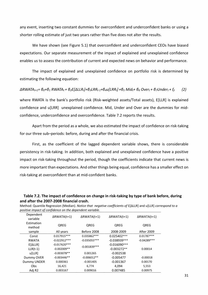
31

any event, inserting two constant dummies for overconfident and underconfident banks or using a

shorter rolling estimate of just two years rather than five does not alter the results.

We have shown (see Figure 5.1) that overconfident and underconfident CEOs have biased

expectations. Our separate measurement of the impact of explained and unexplained confidence

enables us to assess the contribution of current and expected news on behavior and performance.

The impact of explained and unexplained confidence on portfolio risk is determined by

estimating the following equation:

∆RWATAt+1= β0+β1 RWATAt + β2E[ΔLLRt]+β3LRRt-1+β4u[LRRt] +β5 Midt+ β6 Overt + β7Undert + ξt (2)

where RWATA is the bank’s portfolio risk (Risk-weighted assets/Total assets), E[LLR] is explained

confidence and u[LRR] unexplained confidence. Mid, Under and Over are the dummies for mid-

confidence, underconfidence and overconfidence. Table 7.2 reports the results.

Apart from the period as a whole, we also estimated the impact of confidence on risk-taking

for our three sub–periods: before, during and after the financial crisis.

First, as the coefficient of the lagged dependent variable shows, there is considerable

persistency in risk-taking. In addition, both explained and unexplained confidence have a positive

impact on risk-taking throughout the period, though the coefficients indicate that current news is

more important than expectations. And other things being equal, confidence has a smaller effect on

risk-taking at overconfident than at mid-confident banks.

Table 7.2. The impact of confidence on change in risk-taking by type of bank before, during and after the 2007-2008 financial crash. Method: Quantile Regression (Median). Notice that negative coefficients of E[ΔLLR] and u[LLR] correspond to a positive impact of confidence on the dependent variable.

Dependent variable

ΔRWATA(t+1) ΔRWATA(t+1) ΔRWATA(t+1) ΔRWATA(t+1)

Estimation method

QREG QREG QREG QREG

sample All years Before 2008 2008-2009 After 2009

Const 0.017915*** 0.035862*** 0.025402*** 0.01787***

RWATA -0.022912*** -0.035055*** -0.038939*** -0.04289***

E[ΔLLR] -0.017620*** -0.001839***

-0.016090*** 0.00014 LLR(t-1) -0.002009** -0.003272**

u[LLR] -0.003078** 0.001265 -0.002538 Dummy OVER -0.003446** -0.006012** -0.005477 -0.00018

Dummy UNDER 0.000361 -0.001405 -0.001367 0.00170

Obs 16,421 6,774 4,094 5,553

Adj R2 0.003167 0.009016 0.007485 0.00975

32

Finally, during the financial crisis there were no significant differences between bank types in the

reaction of risk-taking.24 However, the coefficients of the dummies for underconfidence and

overconfidence indicate that the relationship between confidence and risk-taking is not linear when

we switch between types of bank. Surprisingly, the intercept of the relationship between

confidence and change in risk is lowest at overconfident banks.25 While by definition the level of

loss reserves is lower (confidence is greater) at overconfident banks, these banks also show the

lowest intercept in the estimated relation between confidence and risk. In other words, banks with

lower reserves (greater confidence) tend to show an increase in risk the next year – ΔRWATA(t+1)

– since the coefficient of reserves is negative. But at the same time overconfident banks have an

idiosyncratic tendency not to increase risk (their dummy is negative). It follows that the overall

impact on risk-taking by overconfident CEOs depends on the relative weights of these two

countervailing effects; and analogously for underconfident banks.

Hence, to estimate the overall impact of confidence on risk-taking for the three types of

bank, we performed another exercise as well, estimating the level of risk-taking by overconfident

and underconfident banks using alternatively the coefficients estimated with the mid-confident

sample only, and samples including the mid-confident as well as the overconfident or

underconfident respectively. The difference between the estimated values of the dependent

variable for these alternative samples reflects the contribution of overconfident or underconfident

banks to risk-taking. The results are reported in Figure 7.1.

Consistently with the foregoing, these results show that overconfident banks do not take on

more risk than the mid-confident. This suggests that overconfident banks may not have been crucial

to bringing about the conditions that led to the financial crash, or at any rate no more than the mid-

confident. Next, we investigate whether this conclusion extends to lending and leverage behavior.

24 The results (not reported here) show that most of the above conclusions apply also to the level of risk-taking, not only the variation. 25 These results hold when we use Robust Least Squares instead of Quantile regression.

33

Figure 7.1 Contribution to risk-taking by type of bank

Estimated equation: RWATAt=β0+ (1+β1 )RWATAt-1 + β2E[LLRt-1] + β3ULLRt-1 +ξt

The estimates are obtained by quantile regression. Observations: 87540. Huber Sandwich Standard Errors & Covariance. Sparsity method: Kernel (Epanechnikov) using residuals. Bandwidth method: Hall-Sheather, bw=0.021881

In (a) the blue (red) dots indicate the estimated values of the level of risk-taking for overconfident (mid-confident) banks using the coefficients estimated with the mid-confident banks. The corresponding lines in (b) refer to comparison between underconfident and mid-confident banks.

(a) (b)

Overconfident Underconfident

7.2 The effects on lending and leverage

Hypothesis 5 posits that more confident banks are more willing to lend, because they are more

optimistic about the success of projects. In addition, banks that expand lending more sharply are

more likely to face capital constraints, so they are also more heavily indebted.

Table 7.3 shows that confidence does have significant effects on banks’ lending, leverage, and

proportion of short-term funding. An increase in confidence leads them to expand lending, increase

leverage, and augment the proportion of deposits and short-term funding.26 However, there are

some interesting differences. While lending and the deposit and short-term funding ratios are

affected by both current news and expectations, leverage is affected only by current news. The

26 We also ran this regression with the ratio between short-term and long-term debt as dependent variable, and the

results are similar.

34

correlation between confidence and the dependent variables in Table 7.3 is lower for overconfident

than mid-confident banks. So we ran exercises similar to those reported in Figure 7.1, with results

qualitatively similar to those for portfolio risk (see Appendix). The overall impact of confidence on

lending and leverage is smaller for overconfident than mid-confident bank CEOs. Thus the previous

conclusions on risk-taking also extend to the other behavioral variables. It follows that, in contrast

with most of the literature on overconfidence, the largest contribution to the increase in risk,

lending and leverage came from mid-confident rather than overconfident bank CEOs.

Table 7.3 The impact of confidence on changes in lending, leverage and short-term funding by type of bank. Method: Quantile Regression (Median). NOTICE THAT negative coefficients of E[ΔLLR] and u[LLR] correspond to a positive impact of confidence on the dependent variable.

Dependent variable ∆ GL(t+1) ΔLog(Y_L1(t+1)) ∆ (DEP ST_FUND/TA)(t+1) Estimation method QREG QREG QREG

sample All years All years All years

Const 0.013624*** 0.171099*** 0.06309*** GL 0.013391*** - -

Log(Y_L1) - -0.068610*** - ∆ (DEP ST_FUND/TA) - - -0.06996***

E[ΔLLR] -0.154771*** -0.035695** -0.00078*** LLR(t-1) -0.011361*** -0.006323**

u[LLR] -0.032081*** -0.002811 Dummy OVER -0.029690*** -0.015686*** -0.00433***

Dummy UNDER -0.009445** -0.007915 0 Obs 19340 19325 38552

Adj R2 0.027211 0.019102 0.01570

To summarize our results on banking behavior, we have shown that risk, lending and leverage all

increase with confidence, but that the relationships are not linear. Overconfident CEOs did not have

a greater impact than others on the increases in risk, lending and leverage. On the contrary, the

sharpest rise in these variables can be attributed to mid-confident CEOs. And these results hold also

when we define the overconfident as the bottom 20% of the distribution of the ratio of loan loss

reserves to gross loans.

35

7.3 The effects on performance

Finally, we investigated the impact of confidence on banks’ performance, gauged by two indicators:

return on average assets (ROAA) and the ratio of non-performing loans to total loans (NPL); other

indicators of performance (e.g. ROE or operating profits) produce similar conclusions.

Table 7.4. The impact of confidence on change in ROAA by type of bank before, during and after the 2007-2008 financial crash. Method: Quantile Regression (Median). Notice that negative coefficients of E[ΔLLR] and u[LLR] correspond to a positive impact of confidence on the dependent variable.

Dependent variable

ΔROAA(t+1) ΔROAA(t+1) ΔROAA(t+1) ΔROAA(t+1)

Estimation method

QREG QREG QREG QREG

sample All years Before 2008 2008-2009 After 2009

Const 0.17108*** 0.10633*** 0.31374*** 0.15137*** ROAA -0.20601*** -0.14909*** -0.50402*** -0.18112***

E[ΔLLR] -0.17637*** 0.02174***

-0.54665** 0.10503 LLR(t-1) 0.00287 -0.02554 0.00736 u[LLR] 0.05150*** 0.12423*** -0.13732 0.01554

Dummy OVER -0.1201*** -0.12750*** -0.11229*** -0.03962** Dummy UNDER -0.03805*** -0.01286 -0.10148 -0.04626***

Obs 15,601 8,282 3,059 4,260

Adj R2 0.05523 0.04732 0.12747 0.05338

We established above (Tables 7.2 and 7.3) that an increase in confidence increases portfolio risk. So

we would expect to find a similar relationship between confidence and profitability, and in fact there

is a negative correlation between estimated reserves E[ΔLLR] and ΔROAA (see Table 7.4). At the

same time, however, banks with higher u[LLR]>0 (i.e. those that were more pessimistic about the

future) got better results. And Table 7.4 shows that before the crisis the less confident banks got

the best results, whereas reserves were correlated negatively with ROAA during the crisis and

positively after it. In any case, the correlation between confidence and profitability is lower at

overconfident than at mid-confident banks, indicating that here too non-linearity prevails, and that

in general overconfidence does not pay. This result is confirmed by the analysis of the overall impact

of confidence on profitability reported in Figure 7.2.

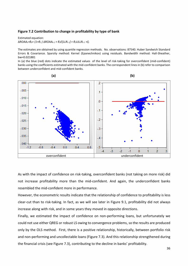
36

Figure 7.2 Contribution to change in profitability by type of bank

Estimated equation: ΔROAAt=β0+ (1+β1 ) ΔROAAt-1 + β2E[LLRt-1] + β3ULLRt-1 +ξt

The estimates are obtained by using quantile regression methods. No. observations: 87540. Huber Sandwich Standard Errors & Covariance. Sparsity method: Kernel (Epanechnikov) using residuals. Bandwidth method: Hall-Sheather, bw=0.021881

In (a) the blue (red) dots indicate the estimated values of the level of risk-taking for overconfident (mid-confident) banks using the coefficients estimated with the mid-confident banks. The correspondent lines in (b) refer to comparison between underconfident and mid-confident banks.

(a) (b)

overconfident underconfident

As with the impact of confidence on risk-taking, overconfident banks (not taking on more risk) did

not increase profitability more than the mid-confident. And again, the underconfident banks

resembled the mid-confident more in performance.

However, the econometric results indicate that the relationship of confidence to profitability is less

clear-cut than to risk-taking. In fact, as we will see later in Figure 9.1, profitability did not always

increase along with risk, and in some years they moved in opposite directions.

Finally, we estimated the impact of confidence on non-performing loans, but unfortunately we

could not use either QREG or robust LS owing to convergence problems, so the results are produced

only by the OLS method. First, there is a positive relationship, historically, between portfolio risk

and non-performing and uncollectable loans (Figure 7.3). And this relationship strengthened during

the financial crisis (see Figure 7.3), contributing to the decline in banks’ profitability.

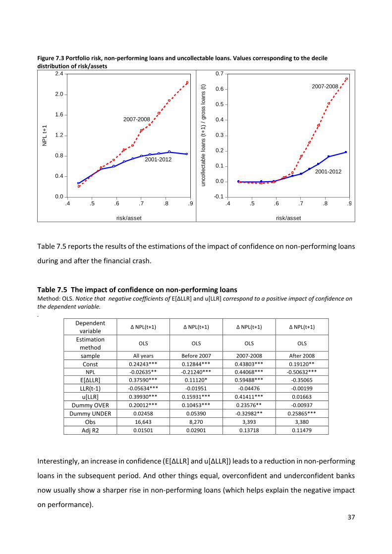
37

Figure 7.3 Portfolio risk, non-performing loans and uncollectable loans. Values corresponding to the decile distribution of risk/assets

0.0

0.4

0.8

1.2

1.6

2.0

2.4

.4 .5 .6 .7 .8 .9

risk/asset

NP

L t

+1

2007-2008

2001-2012

-0.1

0.0

0.1

0.2

0.3

0.4

0.5

0.6

0.7

.4 .5 .6 .7 .8 .9

risk/asset

uncollecta

ble

loans (

t+1)

/ gro

ss loans (

t) 2007-2008

2001-2012

Table 7.5 reports the results of the estimations of the impact of confidence on non-performing loans

during and after the financial crash.

Table 7.5 The impact of confidence on non-performing loans Method: OLS. Notice that negative coefficients of E[ΔLLR] and u[LLR] correspond to a positive impact of confidence on the dependent variable. .

Dependent variable

∆ NPL(t+1) ∆ NPL(t+1) ∆ NPL(t+1) ∆ NPL(t+1)

Estimation method

OLS OLS OLS OLS

sample All years Before 2007 2007-2008 After 2008

Const 0.24243*** 0.12844*** 0.43803*** 0.19120**

NPL -0.02635** -0.21240*** 0.44068*** -0.50632***

E[ΔLLR] 0.37590*** 0.11120* 0.59488*** -0.35065

LLR(t-1) -0.05634*** -0.01951 -0.04476 -0.00199

u[LLR] 0.39930*** 0.15931*** 0.41411*** 0.01663

Dummy OVER 0.20012*** 0.10453*** 0.23576** -0.00937

Dummy UNDER 0.02458 0.05390 -0.32982** 0.25865***

Obs 16,643 8,270 3,393 3,380

Adj R2 0.01501 0.02901 0.13718 0.11479

Interestingly, an increase in confidence (E[ΔLLR] and u[ΔLLR]) leads to a reduction in non-performing

loans in the subsequent period. And other things equal, overconfident and underconfident banks

now usually show a sharper rise in non-performing loans (which helps explain the negative impact

on performance).

38

We also evaluated the overall effect of confidence on the increase in non-performing loans. The

results (not reported here) indicate that non-performing loans increase with confidence, but the

relationship is not significant either before or during the 2008-2009 financial crisis, bolstering our

earlier conclusion of a weak relationship between confidence and performance. The fact is that

performance is not a decision variable for banks but is determined ex post and depends not only on

CEOs’ decisions but also on macroeconomic conditions and other determinants not directly related

to confidence. By contrast, a bank’s portfolio risk, lending and leverage depend more closely on the

CEO’s confidence. In Section 9 we provide additional evidence on the relationship between

confidence and performance.

8. ROBUSTNESS CHECKS

First, we checked whether the results on the determinants of confidence are robust to other

estimation methods. Specifically, we ran the econometric analysis by both the OLS and the robust

LS methods. Quantile regression and robust least squares assign less weight than OLS to the fat tails.

These checks showed that the results do not depend on the specific econometric method adopted

(see Appendix A1).

The foregoing analysis proxied confidence by loan loss reserves. As a first robustness check, we take

as proxies the ratio of loan loss provisions to gross loans and the composite Index 4. The results of

these estimations are qualitatively similar (see Appendix A2). However, these results suggest that

loan loss reserves is a better indicator of confidence than the alternative proxies.

Since listed banks are assumed to be more subject to market discipline and are also likely to differ

in other respects, we tested the determinants of confidence for listed and unlisted banks separately.

The results (Appendix A3) show that unlisted banks react more to balance sheet determinants of

confidence, and listed banks react more to macroeconomics and stock market conditions.

We also tested whether the determinants of confidence are robust to different definitions of

overconfidence and underconfidence: specifically, defining overconfident and underconfident

banks as respectively the bottom and top 20% of the distribution of loan loss reserves. The results

are qualitatively similar to those produced by the narrower definition of overconfidence and

underconfidence (see Appendix A5), and also using this alternative measures of over and

underconfidence the impact on portfolio risk and performance are similar (Appendix 6).

39

It is remarkable to notice that the main relationships between confidence, risk and performance of

the banks hold also when we perform a more complex estimation of the link between economic

results (ROAA), confidence and assets’ risk, which takes account of the feedback effects among

these variables (see Appendix A7).

Finally, we addressed how “confidence” differs from risk aversion. We used two indicators of risk

aversion: Risk-weighted assets/Liquid assets and Risk-weighted assets/LLRxGross loans, assuming

that the higher they are, the lower is the bank’s degree of risk aversion. The results of the

correlations between loan loss provisions and the two indicators (reported in the Appendix A8)

show no strong correlation between confidence and risk aversion, although more confident banks

are also less risk-averse. And the estimations of the residuals of LLR confirm that risk aversion and

confidence, although correlated, capture different phenomena.

9. The optimal degree of confidence in banking

Puri and Robinson (2007) examine the effects of moderate and extreme optimism in several

contexts involving individual choice, concluding that “a moderate amount of optimism can be

positive; it is associated with good financial habits and prudent choices”. Campbell et al. (2011),

studying non-financial firms, provide empirical evidence that there is an interior optimum level of

managerial optimism that maximizes firm value.

Here we address an analogous question: Does there exist some degree of confidence that

maximizes a bank’s value? And, as a follow-up, is this degree of confidence socially desirable?

Addressing these issues is no easy task. The optimal degree of confidence may change according

to the economic conditions and the nature of the bank.

Figure 9.1 Portfolio risk and return to American banks by decile

40

Figure 9.1 shows that the risk/return combination is positive both before and after the crisis, but

that precisely in 2008-2009 the relationship between risk and return is mainly negative. It follows

that the degree of confidence that maximizes the value of the bank is very different in the two cases.

Yet the data reported in Figure 9.2 show that the relationships between confidence and both risk

and return are non-linear.

Figure 9.2 Confidence, estimated risk and return for American banks by decile. Period 2000-2013. (LLR= Loan loss reserves/Gross loans, ROAA=Return on average assets. Risk= Risk weighted assets/Total assets)

.54

.56

.58

.60

.62

.64

.66

.68

0.80

0.84

0.88

0.92

0.96

1.00

1.04

1.08

0.5 1.0 1.5 2.0 2.5 3.0

LLR(t-1)

Risk(t-1)

ROAA(t)

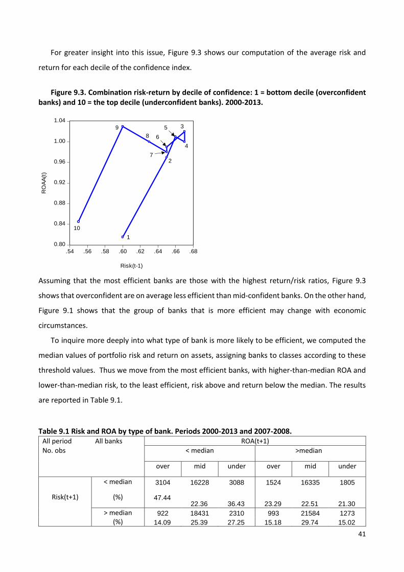
41

For greater insight into this issue, Figure 9.3 shows our computation of the average risk and

return for each decile of the confidence index.

Figure 9.3. Combination risk-return by decile of confidence: 1 = bottom decile (overconfident

banks) and 10 = the top decile (underconfident banks). 2000-2013.

0.80

0.84

0.88

0.92

0.96

1.00

1.04

.54 .56 .58 .60 .62 .64 .66 .68

Risk(t-1)

RO

AA

(t)

10

9

8

7

6

5

4

3

2

1

Assuming that the most efficient banks are those with the highest return/risk ratios, Figure 9.3

shows that overconfident are on average less efficient than mid-confident banks. On the other hand,

Figure 9.1 shows that the group of banks that is more efficient may change with economic

circumstances.

To inquire more deeply into what type of bank is more likely to be efficient, we computed the

median values of portfolio risk and return on assets, assigning banks to classes according to these

threshold values. Thus we move from the most efficient banks, with higher-than-median ROA and

lower-than-median risk, to the least efficient, risk above and return below the median. The results

are reported in Table 9.1.

Table 9.1 Risk and ROA by type of bank. Periods 2000-2013 and 2007-2008. All period All banks ROA(t+1) No. obs < median >median

over mid under over mid under

< median 3104 16228 3088 1524 16335 1805

Risk(t+1) (%) 47.44 22.36 36.43 23.29 22.51 21.30

> median 922 18431 2310 993 21584 1273

(%) 14.09 25.39 27.25 15.18 29.74 15.02

42

2007-2008 All banks ROA(t+1)

< median >median

over mid under over mid under

< median 723 2513 267 237 1854 137

Risk(t+1) (%) 48.07 20.51 31.34 15.76 15.13 16.08

> median 374 5550 354 170 2334 94

(%) 24.87 45.30 41.55 11.30 19.05 11.03

As expected, a third of the mid-confident banks are in the high risk-high return group but only 15%

of the overconfidents. By contrast, 47% of the latter and only 22% of the former are in the low risk-

low return group. The proportion achieving greatest efficiency (ROA>median and Risk<median) is

practically the same for all three types. Finally, 25% of the mid-confident but only 14% of the

overconfident belong to the inefficient combination (ROA<median and Risk>median), suggesting

that the former may have suffered greater losses during the financial crisis. The results reported in

Table 9.1 support this conclusion. The crisis of 2007-2008 pushed a larger proportion of the mid-

confident from the high risk-high return to the high risk-low return. A similar result holds if we

consider the variation rather than the level of risk and return (see Table 9.2).

Table 9.2 Variation in risk and ROA by type of bank. Periods before 2007 and 2007-2008.

2007-2008 All banks ΔROA(t+1)

< median >median

over mid under Over mid under

< median 378 5068 284 226 1890 162

ΔRisk(t+1) (%) 33.19 43.31 35.68 19.84 16.15 20.35

> median 322 3123 222 213 1621 128

(%) 28.27 26.69 27.89 18.70 13.85 16.08

Before 2007 All banks ΔROA(t+1)

< median >median

over mid under over mid under

< median 529 6360 526 486 6566 645

ΔRisk(t+1) (%) 21.69 20.15 21.26 19.93 20.80 26.07

> median 732 8540 589 692 10098 714

(%) 30.01 27.06 23.81 28.37 31.99 28.86

Our evidence, then, does not support earlier works (e.g., Ho et al., 2016) that found overconfident

banks had a higher risk profile before the crisis and were hit harder by it. Instead, on our evidence,

the mid-confident banks took on more risk before the crisis and suffered more serious losses during

it.

10. Concluding remarks

43

We inquired into the role of confidence and overconfidence in shaping the behavior and

performance of US banks before, during and after the financial crash of 2007-2008. Developing new

indicators of confidence and overconfidence, based on loan loss provisions, we have shown that

more confident banks are more willing to take risk and are more heavily indebted. But in our study

the relationship between confidence and risk-taking is not linear: as the bank’s level of confidence

rises, risk, lending and leverage all increase less sharply, rising less among overconfident than among

mid-confident banks. Moreover, our evidence indicates that banks with an intermediate degree of

confidence played a greater role in the increase in banking risk in the run-up to the 2007-2008

financial crisis, and that these banks also suffered the most severe losses in its wake. This reflects

the fact that prior to the crisis mid-confident CEOs reacted more strongly to good news, while the

overconfident were more persistent in their beliefs and did not overreact to good news during the

cyclical upswing. In other terms, our findings do not support the thesis that overconfidents

overreact to good news and underreact to bad (Daniel and Hirshleifer, 2015). Rather, we find that

overconfident CEOs underweight both good and bad news. In addition, we have assessed the impact

of current news and expectations on banks’ risk-taking, lending, leverage and performance, finding

that current news affects both behavior and performance more strongly than expected

developments. In addition, our evidence indicates that in a period of crisis expectations lose their

explanatory power and only current news shapes banking behavior. In any case, however, mid-

confident and overconfident bank CEOs do not differ too greatly in expectations for the future.

Finally, we asked whether there exists some level of confidence that maximizes the value of the

bank. Our conclusion is that there may actually exist more than one level of confidence that

maximizes expected return relative to risk, and that this level depends on the characteristics of the

bank and on general economic conditions. This is because the relationship between risk and return

differs drastically between good and bad times. In any case, our results suggest that overconfidence

never leads to an efficient combination of risk and return, while both underconfidence and mid-

confidence may be optimal, depending on the economic circumstances.

The essential conclusion of this study is that the primary factor in creating the conditions of the

financial crash of 2007-2008 and determining its effects was the evolution of the confidence and

behavior of average banks, the bulk of the banking system. This implies that in order to attenuate

the impact of a financial crisis, it is more important to prevent overconfidence and excessive risk-

taking by the mass of ordinary economic agents than to curb the “irrational exuberance” of a few.

44

References

Adrian, T. and Shin, H. S. (2011), Financial Intermediary Balance Sheet Management, Federal Reserve Bank

of New York Staff Reports no. 532.

Adrian, T. and Shin, H. S. (2013), Procyclical Leverage and Value-at-Risk, Systemic Risk Center, London School

of Economics, Discussion Paper No 1.

Ahmed, A., Takeda, C., & Thomas, S. (1999). Bank loan loss provisions: A reexamination of capital management, earnings management, and signalling effect. Journal of Accounting and Economics, 28(1), 1–25. Akerlof, G. A., Shiller, R. J. (2009), Animal Spirits, Princeton University Press, pp. 230.

Balla, E., Rose, M.J. and Romero, J. (2012), Loan Loss Reserve Accounting and Bank Behavior, The Federal

Reserve Bank of Richmond Economic Bulletin, 12-03, pp. 1-4.

Barberis, N. 2013. Psychology and the financial crisis of 2007—2008. In M. Haliassos (ed.), Financial

innovation: Too much or too little? MIT Press.

Barberis, N. and Thaler, R. (2003), A survey of behavioral finance, in Handbook of the Economics of Finance, Vol. 1, Part B, Elsevier, p. 1053–1112. !_____ __ E__ #___ ___ > __ ___ __ G ____ (_== 7)_ _> ,___ _ +_ ____ #___ ______ ._____

_ / ____ __ *_____ __ 6= _ 5@< _569_ Beatty, A., & Liao, S. (2009). Regulatory Capital Ratios, Loan Loss Provisioning and Pro-cyclicality. Working Paper Available at: http://www.ssrn.com. Beatty, A., & Liao, S. (2015). Does Loan Loss Provision Timeliness Affect the Accuracy, Informativeness, and

Predictability of Analyst Provision Forecasts? Working paper, Fisher College of Business, The Ohio State

University.

Beltratti and Stulz (2012) The credit crisis around the globe: Why did some banks perform better? Journal of

Financial Economics 105, 1–17.

Ben-David, I., Graham, J.R., Harvey, C. R. (2007). Managerial Overconfidence and Corporate Policies, NBER Working Paper 13711.

Ben-David, I., Graham, J. R., Harvey, C. R., 2013. Managerial miscalibration. Quarterly Journal of Economics 128, 15. Campbell, T.C., Gallmeyer, M., Johnson, S.A., Rutherford, J., Stanley, B.W. (2011). CEO optimism and forced turnover. Journal of Financial Economics, 101(3), 695–712. Bikker, J., & Metzemakers, P. (2005). Bank provisioning behavior and procyclicality. International Financial Market, Institutions, and Money, 15(2), 141–157.

Brunnermeier, M. K. (2009) , “Deciphering the Liquidity and Credit Crunch 2007-2008”. Journal of Economic

Perspectives 23: 77-100.

Calomiris, C. W. (2008), The Subprime Turmoil: What’s Old, What’s New, and What’s Next, Paper presented

at the 9th Jacques Polak Annual Research Conference Hosted by the International Monetary Fund

Washington, DC─November 13-14, 2008.

45

Cheng, I., S. Raina, and W. Xiong (2014). Wall Street and the housing bubble. American Economic Review 104

(9), 2797–2829.

Chuang, W., Lee, B. (2006), An empirical evaluation of the overconfidence hypothesis, Journal of Banking and

Finance, 30: 2489-2515.

Daniel, K. and D. Hirshleifer (2015), Overconfident Investors, Predictable Returns, and Excessive Trading,

Journal of Economic Perspectives, 29 (4), 61–88.

Daniel, K., D. Hirshleifer, and A. Subrahmanyam (1998). Investor psychology and security market under- and

overreactions. Journal of Finance 53 (6), 1839–1885.

Daniel, K. and S. Titman (1999), Market Efficiency in an Irrational World. Financial Analysts Journal. Vol. 55

(6), 28-40.

Danielsson, J., Shin, H. S. and Zigrand, J.P., (2011), Balance Sheet Capacity and Endogenous Risk, The Paul

Woolley Centre, Discussion Paper n. 665.

De Grauwe, P. (2012). Booms and busts in economic activity: A behavioral explanation, Journal of Economic Behavior & Organization, 83, 484– 501 Delis, M. D., Hasan, I., Tsionas, E. G. (2014), The risk of financial intermediaries, Journal of Banking & Finance, 44, 1–12.

Demirguc—Kunt, K. and Huizinga, H. (2010), Bank activity and funding strategies: The impact on risk and

returns, Journal of Financial Economics, 98, 626–650.

Demyanyk, Y. and Van Hemert, O. (2011), Understanding the Subprime Mortgage Crisis, Review of Financial

Studies, 24, 1848-1880.

Diamond, D. W. and Rajan, R. (2009), The Credit Crisis: Conjectures about Causes and Remedies, National

Bureau of Economic Research, Working Paper 14739.

Eisenbach, T. M. and Schmalz, M. C. (2015), Anxiety, Overconfidence, and Excessive Risk-Taking , Federal

Reserve Bank of New York, Staff Report No. 711.

El Sood, H.A. (2012), Loan loss provisioning and income smoothing in US banks pre and post the financial

crisis, International Review of Financial Analysis 25: 64–72.

Engle R.F. and Hendry D.F. (1993) Testing Superexogeneity and Invariance in Regression Models, in “Journal

of Econometrics” 1-2, 3-53.

Fahlenbrach, R., Prilmeier, R., Stulz, R., 2012. This time is the same: using bank performance in 1998 to explain

bank performance during the recent financial crisis. Journal of Finance 67, 2139–2185.

Fonseca, A.R. and González, F. (2008), Cross-country determinants of bank income smoothing by managing loan-loss provisions, Journal of Banking & Finance, 32 (2), 217-228.

46

Foote, C. L., K. S. Gerardi, and P. S. Willen (2012). Why did so many people make so many ex post bad

decisions? The causes of the foreclosure crisis. NBER Working Paper 18082.

Fostel, A. and Geanakoplos, J. (2008), Leverage Cycles and the Anxious Economy, American Economic Review

2008, 98:4, 1211–1244.

Geanakoplos, J. (2010), The Leverage Cycle, Cowles Foundation Discussion Paper n. 1715R.

Gennaioli, N., Y. Ma, and R. Vishny (2015a), Expectations and Investment, Working Paper, May.

Gennaioli, N., A. Shleifer, and R. Vishny (2015b), Neglected Risks: The Psychology of Financial Crises, American

Economic Review, 105(5): 310–314.

Glaser, M., Langer, L., and Weber, M. (2005), Overconfidence of professionals and lay men: Individual

differences within and between tasks, Working Paper, University of Manheim.

Glaser, M., and Weber, M. (2007), Overconfidence and trading volume, Geneva Risk and Insurance Review,

32: 1-36.

Goel, A. M., Thakor, A. V., 2008. Overconfidence, CEO selection, and corporate governance. Journal of

Finance 63, 2737–2784.

Gary B. Gorton, G.B. (2008), THE PANIC OF 2007, NBER, Working Paper n. 14358.

Ho, P., Huang, C., Lin, C., Yen, J. (2016), CEO overconfidence and financial crisis: Evidence from bank lending

and leverage. Journal of Financial Economics, Forthcoming.

International Monetary Fund (2014), Global Financial Stability Report: Risk Taking, Liquidity, and Shadow

Banking—Curbing Excess while Promoting Growth, Ch 3.

Jonsson, A., and Allwood, C.M. (2003). Stability and variability in the realism of confidence judgments over

time, content domain, and gender, Personality and Individual Differences 34, 559–574.

Kanagaretnam, K., Lobo, G., & Mathieu, R. (2003). Managerial incentives for income smoothing through bank

loan loss provisions. Review of Quantitative Finance and Accounting, 20(1), 63–80.

Kim, D., Santomero, A.M. (1993). Forecasting required loan loss reserves. Journal of Economics and Business

45, 315–329.

Kindleberger, C. P. (2005), Manias, Panics, and Crashes, John Wiley and Sons, pp. 355.

Klayman, J., Soll, J. B., Gonz´ales-Vallejo, C., and Barlas, S. (1999), Overconfidence: It depends on how, what,

and whom you ask, Organizational Behavior and Human Decision Processes 79, 216–247.

Leventis, S., Dimitropoulos, P.E., and Anandarajan, A. (2011), Loan Loss Provisions, Earnings Management and Capital Management under IFRS: The Case of EU Commercial Banks, J Financ Serv Res (2011) 40:103–122. Levine, R. (2010), An Autopsy of the U.S Financial System, National Bureau of Economic Research, Working

Paper n. 15956.

47

Liu, C., & Ryan, S. (2006). Income smoothing over the business cycle: Changes in banks’ coordinated management of provisions for loan losses and loan charge-offs from the pre-1990 bust to the 1990s boom. The Accounting Review, 81(2), 421–441.

Ma, Y. (2014), Bank CEO Optimism and the Financial Crisis, Harvard University, Working paper.

Malmendier, U. & Tate, G. (2005), ‘Ceo overconfidence and corporate investment’, Journal of Finance 60 (6),

2661–2700.

Minsky, P. H. (1992). The Financial Instability Hypothesis. The Levy Economics Institute of Bard College,

Working Paper N. 74.

Niu, J., 2010. The effect of CEO overconfidence on bank risk taking. Economics Bulletin 30, 3288–3299.

Niu, J., 2014. CEO Overconfidence and Bank Risk Taking. Working paper.

Odean, T. (1998). Volume, Volatility, Price, and Profit When All Traders Are Above Average. The Journal of

Finance, Vol. 53 (6), 1887-1934.

Palumbo, M. G., Parker, J. A., 2009. The integrated financial and real system of national accounts for the

United States: does it presage the financial crisis? American Economic Review 99, 80–86.

Puri, M., Robinson, D.T. (2007), Optimism and economic choice, Journal of Financial Economics, 86, 71–99. Rajan, R. G. (2005), HAS FINANCIAL DEVELOPMENT MADE THE WORLD RISKIER?, NBER, Working Paper n.

11728.

Reinhart, C.M. and Rogoff, K.S. (2009), This Time is Different, Princeton University Press, pp. 463.

Sandroni, A., Squintani, F. (2004), A Survey on Overconfidence, Insurance and Self-Assessment Training

Programs.

Schularick, M. and Alan M. Taylor, A. M. (2010), Credit Booms Gone Bust: Monetary Policy, Leverage Cycles and Financial Crises, 1870–2008, NBER, Working Paper No. 15512. Schrand, C.M. and Zechman, S.L.C. (2012), Executive overconfidence and the slippery slope to financial misreporting, Journal of Accounting and Economics, 53: 311-329.

Shiller, R. J. (2005), Irrational Exuberance, Princeton University Press, pp. 304.

Sironi, A. and Suntheim, F. (2012), CEO Overconfidence in Banking, mimeo.

Taylor, A. M. (2012), The Great Leveraging, mimeo. Thakor, A. (2014), Lending Booms, Smart Bankers and Financial Crises. Working paper. West, R. F., and Stanovich, K. E. (1997), The domain specificity and generality of overconfidence: individual differences in performance estimation bias, Psychonomic Bulletin and Review 4, 387–392.

48

Appendix

A1. Robustness of the estimation method (appendix to section 5 of the text)

The tails of the regression residuals of any equation based on balance-sheet items are particularly fat (Kurtosis on the order of 1000, as against 3 in normal distributions). This phenomenon renders the OLS method ineffective. Possible solutions are quantile regression estimators (QREG) and robust least squares (robust LS). Since in this paper we employed QREG, it will be useful to compare the estimations obtained by QREG, robust LS, and OLS. The equations selected for the comparison are those reported in columns (1) and (2) of Table 5.1 of the text, and the results are shown in Table A1.1. The signs of the significant parameters are usually the same for any estimator, but the QREG estimated parameters generally lie between those obtained by OLS and robust LS. These results support our choice of QREG. The residual distribution Kurtosis of eq. (1) is 1034.826, and the residuals from alternative methods have quite similar Kurtosis.

Table A1.1 Estimation of the determinants of loan loss reserves/gross loans; comparison of regression methods Years: 2001-2013; */**/*** indicate significance at 10/5/1% respectively. Notice that a higher value for the dependent variable corresponds to a lower level of confidence. Hence (apart from the lagged dependent variable) a negative coefficient corresponds to an increase in confidence.

Original equations Eq (1) Table 5.1

Eq (2) Table 5.1

Equation (1) (2) (3) (4) (5) (6) Estimation Method for comparison QREG OLS RobustLS QREG OLS RobustLS Type of sample open open open closed closed closed Regressors / Equations (1) (2) (3) (4) (5) (6)

const -0.03423 0.68986* 0.17512** -0.01783 -0.11218 0.16964** LLR(t-1) -0.06440*** -0.12109*** -0.05890*** -0.05824*** -0.11043*** -0.04625*** LLP(t-1) -0.00135 -0.00828*** -0.00059 0.00255** -0.00397 0.00004 100* UNC -0.06270*** -0.00526*** -0.73700*** -0.27417** -0.01615*** -0.86783*** ∆ GL -0.08140*** -0.02176*** -0.96151*** -0.50676*** -0.05899*** -1.07536*** ∆ (NPL) 0.04208*** 0.08961*** 0.00913*** 0.01561** 0.07901*** 0.00697*** NPL(t-1) 0.01078*** 0.02634*** 0.00107 -0.00176 0.04134*** 0.00432*** LOG(TA(t-1)) 0.00080 0.00001 0.01116*** 0.00592*** -0.00445** 0.00372*** ∆LOG(TA) -0.01299 -0.14369*** 0.13318*** 0.15891 -0.14463*** 0.05813*** LOG(GLTA (t-1)) 0.00469 0.00623 -0.01394*** -0.01244*** -0.01505** -0.01324*** IMP 0.10058*** 0.01501 0.20397*** 0.38963*** -0.10979* -0.02085 TIER1 -0.00014*** 0.00194*** -0.00016*** -0.00034*** 0.00028 -0.00019*** OP(t-1) -0.08332*** -0.07753*** -0.70809*** -0.20593** -0.07116*** -1.10061*** PBT 0.08671*** 0.07634*** 0.70870*** 0.21230** 0.08828*** 1.09953*** ∆(PBT) -0.06781*** -0.06934*** -0.70031*** -0.17999** -0.05905*** -1.09787*** GDP -0.00344*** 0.00010 -0.00121** -0.00098 0.00320 -0.00054 CLIF 0.00117 -0.00476* -0.00102 0.00072 0.00083 -0.00102* LOG(SMK(t-1)) -0.00065 -0.01081 -0.00710 -0.00253 0.02362 -0.00359 ∆LOG(SMK) -0.06763*** -0.09058*** -0.02045*** -0.05759*** -0.13856*** 0.00247 Fed_fund -0.00644*** -0.00693*** -0.00048 -0.00384*** -0.01048*** -0.00016 No. observations: 50,461 50,461 50,461 36,454 36,454 36,454 R-squared/Pseudo R-squared 0.04690 0.11869 0.23156 0.10897 0.10538 0.43243

Qreg= Years: 2001-2013. Qreg = Method: Quantile Regression (Median), Huber Sandwich Standard Errors & Covariance, Sparsity method: Kernel (Epanechnikov) using residuals, Bandwidth method: Hall-Sheather, bw=0.020706, Estimation successfully identifies unique optimal solution; OLS = ordinary least square; RobustLS = Method: Robust Least Squares; M-estimation; M settings: weight=Bisquare, tuning=4.685, scale=MAD (median centered); Huber Type II Standard Errors & Covariance

Our regressions to explain the values of LLR, the ratio of loan loss reserves to gross loans, contain some variables at t that we considered exogenous. In order to verify this hypothesis we employed

49

the procedure suggested by Engle and Hendry (1993), namely estimating an equation (marginal equation) for every variable under examination where all regressors are “predetermined” (instruments) and taking their residuals as additional variables to include in the regressions of LLR. If their coefficients are not significant, the corresponding variables cannot be rejected as exogenous. The marginal equations we used contained only lagged variables, apart from the macroeconomic variables taken at t. The results of the test are reported in column 2 of Table A.1.2: none of these variables proved to be significant, even at the 10% level: “weak exogeneity” cannot be rejected, and the parameters can be regarded as unbiased. In equation 5 of the same table, the variable RWTA at t-1 was introduced as a further explanatory variable for LLR. Its coefficient turned out to be positive and significant, meaning that an increase in asset riskiness reduces confidence, but, at the same time, other coefficients remain almost the same. Unfortunately the number of observations diminishes, since RWTA(-1) is not always available, so in the rest of the paper we continued to prefer the equations without this variable. Interestingly, the inclusion of RWTA at time t gives a coefficient with the “wrong” sign (negative instead of positive), while other coefficients remain almost the same. Table A1.2 Estimation of the determinants of loan loss reserves/gross loans with and without portfolio risk as regressor Years: 2001-2013. Method: Quantile Regression (Median), Huber Sandwich Standard

Errors & Covariance, Sparsity method: Kernel (Epanechnikov) using residuals, Bandwidth method: Hall-Sheather, bw=0.020706, Estimation successfully identifies unique optimal solution; Δ() indicate change; */**/*** indicate significance at 10/5/1% of probability respectively. Notice that a higher value for the dependent variable corresponds to a lower level of confidence. Hence (apart from the lagged dependent variable) a negative coefficient corresponds to an increase in confidence. Dependent Variable: ∆(LLR) ∆(LLR) ∆(LLR) ∆(LLR) ∆(LLR) ∆(LLR) Equation (1) (2) (3) (4) (5)

Type of sample open open open with RWATA among regressors

Open, but same sample as eq(3)

open with risk(6)_asset at t-1 among regressors

Open, but same smple as eq(5)

Fixed effects no no no no no no Estimation Method QREG QREG QREG QREG

-

(Coefficients of BIAS TEST for weak exogeneity variables at t)

- - - -

Regressors / Equations (1) (2) (3) (4) (5) (6)

const -0.03423 -0.03821 0.15712 0.10194 0.20623* 0.28714*** LLR(t-1) -0.06440*** -0.06425*** -0.07301*** -0.07456*** -0.06300*** -0.06099*** LLP(-t-1) -0.00135 -0.00188 -0.00130 -0.00128 0.00105 -0.00001 100* UNC -0.06270*** -0.06141*** -0.09228*** -0.09171*** -0.44927*** -0.45119*** ∆ GL -0.08140*** -0.05432 -0.11084*** -0.11242*** -0.68824*** -0.69044*** ∆ (NPL) 0.04208*** 0.02959 0.04513*** 0.04551*** 0.03255*** 0.03090*** NPL(t-1) 0.01078*** 0.00766 0.02004*** 0.02005*** 0.01814*** 0.01588*** LOG(TA(t-1)) 0.00080 0.00128 0.00398*** 0.00397*** 0.00551** 0.00559*** ∆LOG(TA) -0.01299 -0.09334 -0.01343 -0.01526 0.15251*** 0.15924*** LOG(GLTA (t-1)) 0.00469 0.00945 0.02307*** 0.01136** -0.01312*** 0.00414 IMP 0.10058*** 0.06654 0.03034*** 0.02999*** -0.23536*** -0.20953*** TIER1 -0.00014*** -0.00010 -4.72E-0 0.00011 0 -0.00010* OP(t-1) -0.08332*** -0.08273*** -0.09792*** -0.09604*** -0.27722*** -0.27940*** PBT 0.08671*** 0.08578*** 0.10196*** 0.09985*** 0.27791*** 0.28098*** ∆(PBT) -0.06781*** -0.06637*** -0.07885*** -0.07787*** -0.25533*** -0.25686*** GDP -0.00344*** -0.00360 -0.00233** -0.00234** -0.00183** -0.00233*** CLIF 0.00117 0.00123 0.00027 0.00040 -9.66E-0 -0.00027 LOG(SMK(t-1)) -0.00065 -0.00043 -0.01066 -0.00948 -0.02623*** -0.02859*** ∆LOG(SMK) -0.06763*** -0.07230** -0.06936*** -0.07104*** -0.03700*** -0.03183*** Fed_fund -0.00644*** -0.00649*** -0.00516*** -0.00536*** -0.00241*** -0.00210***

50

RWATA - - -0.04628*** - - - RWATA(t-1) - - - - 0.06267*** - U1 (= resid of estimation of D(GROSS_LOANS)/GROSS_LOANS(-1))

- -0.03204 - - - -

U2(= resid of estimation of D(NPL)

- 0.01187 - - - -

U3 (resid of estimation of DLOG(T_ASSET)

- 0.08039 - - - -

U4 (= resid of estimation of IMPAIRED_LOANX/TOTAL_EQUITY)

- 0.03513 - - - -

U5 (= resid of estimation of TIER_1_REG_CAP_RAT)

- -0.00034 - - - -

No. observations: 50,461 50,386 44,655 44,655 35732 35732

Pseudo R-squared 0.04690 0.04680 0.05249 0.05223 0.15712 0.15648

A2. Other main indicators for confidence (appendix to section 5 of the text)

Since we also considered LLP, the ratio of loan loss provisions to gross loans, as a possible measure of confidence, we estimated some equations relating to the determinants of this variable. Since in over 80% of the cases LLP turns out to be zero, the QREG estimator provides weak results and the robust LS method did not converge. The regressors employed for LLP are the same as for LLR, with LLP(t-1) instead of ∆(LLR(t-1)). LLP is introduced in level and not in ∆, since it is a flow and not a stock variable. The sign of the coefficients of non-performing loans is wrongly negative instead of positive (Table A2.1), while the other main variables have same sign as in the LLR equations. That negative sign of NPL remains even when the LLP regression is limited to the cases in which the dependent variable is different from zero. The same result emerges if the estimation is performed with a QREG with tau=0.8 instead of the usual 0.5.If OLS is used, the NPL parameters turn positive, but the absolute values of the coefficients are in general very high and the kurtosis of the residuals is 1076.6. Table A2.1 Estimation of the determinants of LLP (loan loss provision/gross loans). Years: 2001-2013.

Method: Quantile Regression (Median), Huber Sandwich Standard Errors & Covariance, Sparsity method: Kernel (Epanechnikov) using residuals, Bandwidth method: Hall-Sheather, bw=0.020706, Estimation successfully identifies unique optimal solution; Δ() indicate change; */**/*** indicate significance at 10/5/1% respectively. Notice that a higher value of the dependent variable corresponds to a lower level of confidence. Hence (apart from the lagged dependent variable) a negative coefficient corresponds to an increase in confidence. Dependent Variable: LLP LLP LLP LLP LLP

51

Type of sample Open Open

Open

(Only

LLP/GL>0)

Open, but same smple of eq(3)

close

Fixed effects No no no no no

Estimation Method QREG OLS QREG QREG QREG (tau=0.8)

Regressors / Equations (1) (2) (3) (5) (6)

const -0.01081 4.23068*** 4.03079*** -0.01656* 0.08007 LLR(t-1) -0.00043*** 0.04757*** 0.07033* -0.00069*** 0.00265*** LLP(t-1) -0.11563*** -0.01542** 0.05451 -0.14135*** 0.32943*** 100* UNC 0.03121*** 0.07335*** 0.65139*** 0.02975*** 0.11448***

∆ GL 0.03362*** 0.13322*** -0.13867***

0.03225*** 0.14016***

∆ (NPL) -0.00429 0.15423*** 0.09605*** -0.00498 -0.01754***

NPL(t-1) -0.00556 0.06852*** 0.05459** -0.00595 -0.02034***

LOG(TA(t-1)) 0.00136*** 0.06517*** -0.07370***

0.00127*** 0.00525***

∆LOG(TA) 0.00267 -0.24614***

0.27353** 0.00266 0.00029

LOG(GLTA (t-1)) -0.00068 0.09106*** -0.15788***

-0.00056 -0.00608***

IMP 0.17128** 0.26661*** 0.09641*** 0.17773* 1.12665*** TIER1 4.77E-0** 0.00065*** 0.00309 0.00006** 0.00032***

OP(t-1) -0.82236*** -0.58674***

-0.07747 -0.82502*** -0.71490***

PBT 0.82287*** 0.62221*** 0.09892 0.82552*** 0.71754***

∆(PBT) -0.82036*** -0.56366***

-0.0590 -0.82287*** -0.70568***

GDP -0.00032*** -0.03192***

-0.02591***

-0.00023*** -0.00347***

CLIF 0.00000 -0.03392***

-0.02668***

0.00008 -0.00032

LOG(SMK(t-1)) 0.00000 -0.16090***

-0.12390 0.00022 -0.00985***

∆LOG(SMK) -0.00253*** 0.15570*** 0.32795*** -0.00330*** -0.01308***

Fed_fund -0.00022*** 0.00992*** 0.00073 -0.00021*** -0.00076***

No. observations: 50,553 50,553 6,370 44,737 36,460

Adj Pseudo R-squared 0.09195 0.30295 0.41732 0.08562 0.2722

Table A2.2 reports the equations explaining the three variables, LRR, LLP, INDEX4 for a comparison, of which INDEX4 can be considered an additional alternative to LLR and LLP as a confidence indicator. The variable INDEX4 too is a flow and so did not have to be expressed in ∆; unlike LLR and LLP, it is positively related to confidence, so the parameters of its explanatory equation should normally be of the opposite sign. Unfortunately, while NPL coefficients present the right sign (negative for INDEX4), the variables relating to profits were mostly negative, whereas they should be positively correlated with confidence; the same applikes for all the macroeconomic variables except the fed funds rate. In general, then, all these results favour our choice of LLR as a (negative) indicator of confidence, at least on the base of LLP and INDEX4 explanatory equations. Table A2.2 Estimation of the determinants of INDEX4, and comparison of equations of loss reserves/gross loans and of LLP/gross loans. Years: 2001-2013. Method: Quantile Regression (Median), Huber

Sandwich Standard Errors & Covariance, Sparsity method: Kernel (Epanechnikov) using residuals, Bandwidth method:

52

Hall-Sheather, bw=0.020706, Estimation successfully identifies unique optimal solution; Δ() indicate change; */**/*** indicate significance at 10/5/1% of probability respectively. Notice that higher values LLR and LLP of the dependent variable correspond to a lower level of confidence, while a higher value of INDEX4 corresponds to a higher level of confidenc Dependent Variable: LLR LLP INDEX4

Type of sample open open open

Fixed effects no no no Estimation Method QREG QREG QREG Regressors / Equations (1) (2) (3)

const -0.03423 -0.01081 148.1118*** LLR(t-1) -0.06440*** -0.00043*** - LLP(t-1) - -0.11563*** - INDEX4(t-1) - - -0.54570*** ∆LLR(t-1) -0.00135 - - 100* UNC -0.06270*** 0.03121*** 0.02511 ∆ GL -0.08140*** 0.03362*** 0.33870*** ∆ (NPL) 0.04208*** -0.00429 -0.03371*** NPL(t-1) 0.01078*** -0.00556 -0.01491** LOG(TA(t-1)) 0.00080 0.00136*** 0.00621* ∆LOG(TA) -0.01299 0.00267 1.97296*** LOG(GLTA (t-1)) 0.00469 -0.00068 -0.04761*** IMP 0.10058*** 0.17128** 0.58502*** TIER1 -0.00014*** 4.77E-0** -0.00195*** OP(t-1) -0.08332*** -0.82236*** -0.02888 PBT 0.08671*** 0.82287*** 0.01878 ∆(PBT) -0.06781*** -0.82036*** -0.07108*** GDP -0.00344*** -0.00032*** -0.69318*** CLIF 0.00117 0 -0.46095***

LOG(SMK(t-1)) -0.00065 0 -14.93065***

∆LOG(SMK) -0.06763*** -0.00253*** -2.31330*** Fed_fund -0.00644*** -0.00022*** 0.72881*** RWATA - - - No. observations: 50,461 50,553 50.369

Adj Pseudo R-squared 0.04690 0.09195 0.25830

A3. The difference in the determinants of confidence between listed and unlisted banks (appendix

to section 5 of the text)

The regressions for LLR, estimated separately for listed and unlisted banks, are reported in Table A.3.1. The signs of the coefficients are the same for all the significant parameter values, with the adjustment coefficient for listed companies being higher (by about three times). The estimate for the entire sample of banks is almost the same as that for unlisted banks only. In general, the coefficients of balance-sheet items are higher for unlisted banks and those of macroeconomic variables are higher for listed banks. Closed samples cannot be estimated, since the number of listed banks is too small.

Table A3.1 Estimation of the determinants of loss reserves/gross loans and of LLP/gross loans: Listed and unlisted banks. Years: 2001-2013. Method: Quantile Regression (Median), Huber Sandwich Standard

Errors & Covariance, Sparsity method: Kernel (Epanechnikov) using residuals, Bandwidth method: Hall-Sheather, bw=0.020706, Estimation successfully identifies unique optimal solution; Δ() indicate change; */**/*** and °/°°/** indicate significance at 10/5/1% respectively, where * refers to coefficient significance, ° refers to the significance of the difference with respect to the previous column.

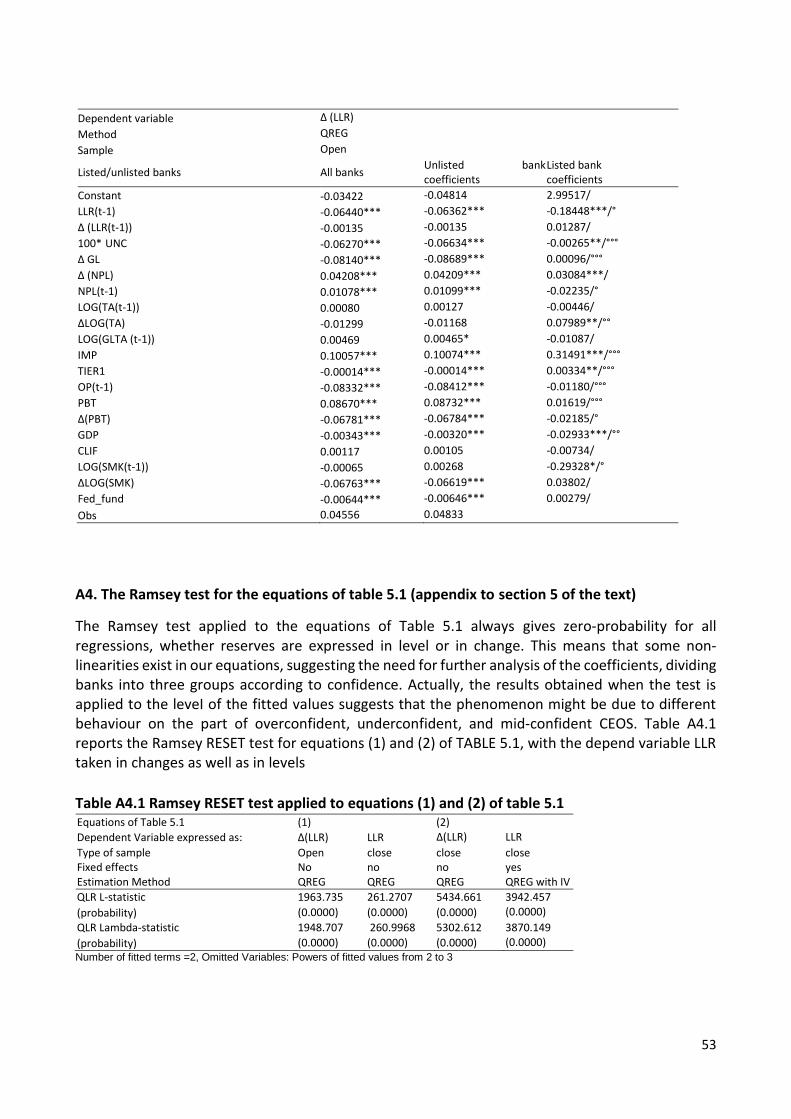
53

Dependent variable ∆ (LLR)

Method QREG

Sample Open

Listed/unlisted banks All banks Unlisted bank coefficients

Listed bank coefficients

Constant -0.03422 -0.04814 2.99517/

LLR(t-1) -0.06440*** -0.06362*** -0.18448***/°

∆ (LLR(t-1)) -0.00135 -0.00135 0.01287/

100* UNC -0.06270*** -0.06634*** -0.00265**/°°°

∆ GL -0.08140*** -0.08689*** 0.00096/°°°

∆ (NPL) 0.04208*** 0.04209*** 0.03084***/

NPL(t-1) 0.01078*** 0.01099*** -0.02235/°

LOG(TA(t-1)) 0.00080 0.00127 -0.00446/

∆LOG(TA) -0.01299 -0.01168 0.07989**/°°

LOG(GLTA (t-1)) 0.00469 0.00465* -0.01087/

IMP 0.10057*** 0.10074*** 0.31491***/°°°

TIER1 -0.00014*** -0.00014*** 0.00334**/°°°

OP(t-1) -0.08332*** -0.08412*** -0.01180/°°°

PBT 0.08670*** 0.08732*** 0.01619/°°°

∆(PBT) -0.06781*** -0.06784*** -0.02185/°

GDP -0.00343*** -0.00320*** -0.02933***/°°

CLIF 0.00117 0.00105 -0.00734/

LOG(SMK(t-1)) -0.00065 0.00268 -0.29328*/°

∆LOG(SMK) -0.06763*** -0.06619*** 0.03802/

Fed_fund -0.00644*** -0.00646*** 0.00279/

Obs 0.04556 0.04833

A4. The Ramsey test for the equations of table 5.1 (appendix to section 5 of the text)

The Ramsey test applied to the equations of Table 5.1 always gives zero-probability for all regressions, whether reserves are expressed in level or in change. This means that some non-linearities exist in our equations, suggesting the need for further analysis of the coefficients, dividing banks into three groups according to confidence. Actually, the results obtained when the test is applied to the leveI of the fitted values suggests that the phenomenon might be due to different behaviour on the part of overconfident, underconfident, and mid-confident CEOS. Table A4.1 reports the Ramsey RESET test for equations (1) and (2) of TABLE 5.1, with the depend variable LLR taken in changes as well as in levels

Table A4.1 Ramsey RESET test applied to equations (1) and (2) of table 5.1 Equations of Table 5.1 (1) (2)

Dependent Variable expressed as: ∆(LLR) LLR ∆(LLR) LLR Type of sample Open close close close Fixed effects No no no yes Estimation Method QREG QREG QREG QREG with IV

QLR L-statistic 1963.735 261.2707 5434.661 3942.457

(probability) (0.0000) (0.0000) (0.0000) (0.0000) QLR Lambda-statistic 1948.707 260.9968 5302.612 3870.149

(probability) (0.0000) (0.0000) (0.0000) (0.0000) Number of fitted terms =2, Omitted Variables: Powers of fitted values from 2 to 3

54

A5. Estimation of the determinants of confidence with dummy variables by category of bank when

the overconfident are defined as below the 20th percentile and the underconfident as above the

80th percentile (appendix to Table 5.5 of section 5 of the text)

Table A5.1 replicates Table 5.5 of the text, identifying overconfident and underconfident banks as

the 20th and 80th percentiles of LLR respectively, instead of 10th and 90th. The results are

qualitatively similar to those of the original table, meaning that the definition of under- and over-

confident need not to be limited to very restricted cases.

Table A5.1: Estimation of the determinants of confidence with dummy variables by category of bank Years: 2001-2013. Method: Quantile Regression (Median), Huber Sandwich Standard Errors & Covariance, Sparsity

method: Kernel (Epanechnikov) using residuals, Bandwidth method: Hall-Sheather, bw=0.020706, IV applied to

dummies for over- and under-confident banks. Estimation successfully identifies unique optimal solution; D() indicate

change; */**/*** refer to the coefficient significance at 10%/5%/1% respectively; and °/°°/°°° refer to the significance

of the difference between the coefficients of overconfidents and underconfidents with respect to mid-confident banks.

Notice that a higher value of the dependent variable corresponds to a lower level of confidence. Hence (apart from the

lagged dependent variable) a negative coefficient of LLR and D(LLR) corresponds to an increase in confidence.

Dependent Variable: ∆(LLR) Type of sample open Fixed effects no Estimation Method QREG mid-confident overconfident underconfident

Constant -0.70507*** -0.53449**/ 0.46233/

LLR(-1) -0.10057*** 0.00792/°°° -0.06849***/°°°

∆ (LLR(-1)) 0.00772 0.01435/ 0.01304/

100* UNC -0.24394*** -0.01120/°°° -0.41748***/°°°

∆ GL -0.34804*** 0.00743/°°° -1.58127***/°°°

∆ (NPL) 0.02123** 0.01571*/ 0.03703***/

NPL(-1) -0.00130 0.00529/ 0.00425/

LOGTA (-1) 0.00840*** -0.00211**/°°° 0.01445**/

∆ LOGTA 0.12698*** 0.01019/°°° 0.18733**/

LOG(GLTA (-1))) 0.00677 -0.00072/ 0.00492/

IMP 0.46828** 0.42647***/ 0.09702***/°

TIER1 0.00052*** -0.00004**/°°° 0.00182***/°

OP(-1) -0.18384*** -0.02955/°°° -0.32765***/

PBT 0.18748*** 0.02876/°°° 0.35499***/°

∆(PBT) -0.14704*** -0.03119/°° -0.31759***/°

GDP -0.00224 0.00144/ -0.01603***/

CLIF 0.00552*** 0.00334**/ -0.00148/

LOG(SMK(-1)) 0.03360** 0.03093**/ -0.03777/

∆LOG(SMK) -0.13124*** -0.08072***/°° 0.03982/°

Fed_fund -0.00744*** -0.00531***/ -0.00632/

Obs. 42,628

Adj Pseudo R-squared 0.15036

55

A6. Effect on performance and risk-weighted assets when the overconfident are below the 20th

percentile and the underconfident above the 80th percentile of the confidence distribution

(appendix to sections 7.1 and 7.3 of the text)

In this appendix we compare the relation between ROAA and risk when the dummies for

overconfident and underconfident banks are identified as the 20th and 80th percentile instead of the

10th and 90th, as in the text (Table A6.1)

Table A6.1. The impact of confidence on change in ROAA and risk weighted assets Method: Quantile Regression (Median). Notice that negative coefficients of E[ΔLLR] and u[LLR] correspond to a positive impact of confidence on the dependent variable.

Dependent variable

ΔROAA(t+1) ΔROAA(t+1) ΔRWATA(t+1) ΔRWATA(t+1)

Estimation method QREG QREG QREG QREG

Identification of over and underconfident banks

10% and 90% quantiles of LLR

20% and 80% quantiles of LLR

10% and 90% quantiles of LLR

20% and 80% quantiles of LLR

sample All years All years All years All years

Const 0.17108*** 0.17593*** 0.02086*** 0.02249***

ROAA -0.20601*** -0.19405*** -0.02494*** -0.02785***

E[ΔLLR] -0.17637*** -0.17303*** -0.01723*** -0.01559***

LLR(t-1) 0.00287 -0.00356 -0.00237*** -0.00083

u[LLR] 0.05150*** 0.04879** -0.00293* -0.00211

Dummy OVER -0.1201*** -0.0939*** -0.00467** -0.00488***

Dummy UNDER -0.03805*** -0.02571* 0.00071 -0.00487***

Obs 15,601 15.981 13,048 13,048

Adj R2 0.05523 0.05692 0.004752 0.004752

Again in this case the values of the parameters are similar, confirming that our results do not depend

on some particular measure of over- and under-confidence.

Table A6.2. The impact of confidence on change in ROAA by type of bank before, during and after the 2007-2008 financial crash. Method: Quantile Regression (Median). Notice that negative coefficients of E[ΔLLR] and u[LLR] correspond to a positive impact of confidence on the dependent variable.

Dependent variable

ΔROAA(t+1) ΔROAA(t+1) ΔROAA(t+1) ΔROAA(t+1)

Estimation method

QREG QREG QREG QREG

sample All years Before 2008 2008-2009 After 2009

Const 0.17108*** 0.10633*** 0.31374*** 0.15137*** ROAA -0.20601*** -0.14909*** -0.50402*** -0.18112*** E[ΔLLR] -0.17637***

0.02174*** -0.54665** 0.10503

LLR(t-1) 0.00287 -0.02554 0.00736 u[LLR] 0.05150*** 0.12423*** -0.13732 0.01554 Dummy OVER -0.1201*** -0.12750*** -0.11229*** -0.03962** Dummy UNDER -0.03805*** -0.01286 -0.10148 -0.04626*** Obs 15,601 8,282 3,059 4,260

Adj R2 0.05523 0.04732 0.12747 0.05338

56

A7. A more complex estimation of the relationship between confidence, risk-weighted assets

(RWATA) and bank’s performance (ROAA) (appendix to section 7 of the text)

A more complete equation for the relationship between RWATA, ROAA and LLR (taken as an inverse

measure of confidence) must take into account that:

1) ∆(RWATA) and ∆(ROAA) are related to their previous level, since after a particularly high

(low) level of this variable, they should move in the opposite direction.

2) There might be positive / negative economies of scale, so the coefficient of LOGTA has to be

considered as an important signal.

3) A favourable GDP scenario increases RWATA and ROAA, owing to a reduction in both

economic risk and in the negative components of banks’ profit-and-loss accounts.

4) The higher the interest rate, the greater the interest margin and the higher the banks’

profits.

5) Measuring capitalization as the Tier1 Regulatory capital ratio TIER1 or total equity /total

assets (EQTA) might influence ROAA positively.

6) The liquidity of assets/liabilities (LIQU and DEP) may influence risk or profits.

7) Under normal conditions, a higher RWATA should correspond to higher ROAA since greater

risk has to be rewarded by a higher return.

The first results from the estimation of RWATA and ROAA are reported in Table A7.1

Table A7.1 Estimation of change in RWATA and ROAA. Years: 2001-2013. Method: Quantile Regression

(Median), Huber Sandwich Standard Errors & Covariance, Sparsity method: Kernel (Epanechnikov) using residuals, Bandwidth method: Hall-Sheather, bw=0.020706, Estimation successfully identifies unique optimal solution; Δ() indicate change; */**/*** indicate significance at 10/5/1% respectively.

Dependent variable ∆ (RWATA) ∆ (ROAA)

equation (1) (2)

const -0.01807*** -0.07709***

ROAA(t-1) -0.00198*** -0.15352***

RWATA(t-1) -0.04902*** 0.24169***

RWATA(t-1)*crisis - -0.08617***

∆ (RWATA(t-1)) -0.09631*** 0.12979***

LOGTA(t-1) 0.00530*** 0.01330***

EQTA(-1) - 0.00148**

LIQU 0.02832*** -

E(∆ LLR(t-1)] -0.00183 -0.00981

LLR(t-2) 0.00160 -0.14363

u[LLR(t-1)] -0.00499*** 0.06831**

NPL(t-1) -0.00099 -

GL(t-1)/TA(t-1) 0.01996*** -

∆ (GDP)*GL(t-1)/TA(t-1) - 0.02325***

GDP(t-1) 0.00326***

∆ (Fed-fund) - 0.01392***

Fed_fund 0.00380*** -

Dummy OVER(t-1) -0.00354* -0.03461***

Dummy UNDER(t-1) 0.00287 0.00461

No. observations 12,526 12,530

Adjusted Pseudo R2 0.03693 0.04485

57

In both equations, the coefficients are as one would expect. Risk and ROAA variations are negatively correlated with their lagged values, the coefficient of LOGTA suggests the presence of scale economies, and the percentage of equity over assets has a positive impact on ROAA. GDP growth exerts a positive effect on RWATA as well as ROAA; the same is true for the interest rate (Fed_fund). The effect of the unexplained component of LLR, i.e. u[LLR(t-1)], on risked assets is negative and highly significant: this means that the more optimistic and confident banks are willing to assume more risk. The increase in risk depends also on the percentage of asset liquidity and of loans. ROAA is positively influenced by RWATA (riskier assets are usually more profitable), but, of course, crisis has a negative impact on this relation. On the other side, u[LLR], which increases ROAA via RWATA, also exerts a direct negative effect on ROAA itself: this might suggest that excessive confidence may be dangerous. The dummy for overconfidence is negative and particularly significant for ROAA, confirming that being overconfident is generally negative for ROAA. The underconfidence dummy is instead never significant.

A8. Risk aversion and confidence (appendix to section 8 of the text)

We used two indicators of risk aversion. Aversion1 is defined as Liquid assets/Risk-weighted assets; Aversion2 is Total loan loss reserves LLR / Risk-weighted assets, i.e. LLR*GL/RWATA). The higher those indicators, the greater the CEO’s risk aversion. The results of the regression between the two proxies of risk aversion and LLR are reported in Table A8.1 Table A8.1 Estimation of change in ROAA and in RWATA. Years: 2001-2013. Method: Quantile Regression

(Median), Huber Sandwich Standard Errors & Covariance, Sparsity method: Kernel (Epanechnikov) using residuals, Bandwidth method: Hall-Sheather, bw=0.020706, Estimation successfully identifies unique optimal solution; Δ() indicate change; */**/*** indicate significance at 10/5/1% of probability respectively.

Dependent variable Log(LLR)

equation (1)

const -0.17559***

log(aversion1) -0.23834***

log(aversion2) 0.02655***

No. observations 41,847

Adjusted Pseudo R2 0.58439

The first figure below shows no strong correlation between confidence and risk aversion, while the second shows a strong positive correlation between risk taking and LLR: the less confident banks are also more highly risk averse. However, the coefficients of both risk-aversion measures in a regression of LLR on the two indicators are highly significant, so we infer that risk aversion and confidence are highly correlated even if the variables capture different phenomena. Fig. A8.1 Loan loss reserves and risk-aversion

58