Conditioning and Aggregating Uncertain Data Streams: Going Beyond Expectations

Thanh Tran, Andrew McGregor, Yanlei Diao,

Liping Peng, Anna Liu

University of Massachusetts, Amherst

Presented by Xin Miao

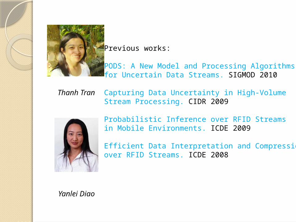
Thanh Tran

Yanlei Diao

Previous works:

PODS: A New Model and Processing Algorithms for Uncertain Data Streams. SIGMOD 2010

Capturing Data Uncertainty in High-Volume Stream Processing. CIDR 2009

Probabilistic Inference over RFID Streams in Mobile Environments. ICDE 2009

Efficient Data Interpretation and Compression over RFID Streams. ICDE 2008

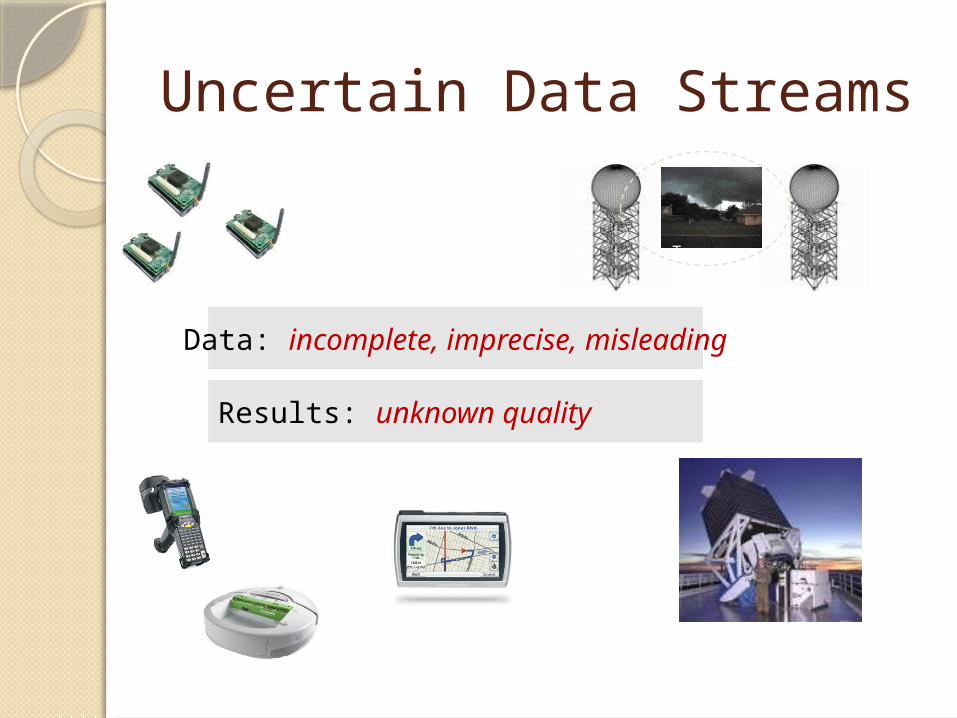
Uncertain Data Streams

TV

Data: incomplete, imprecise, misleading

Results: unknown quality

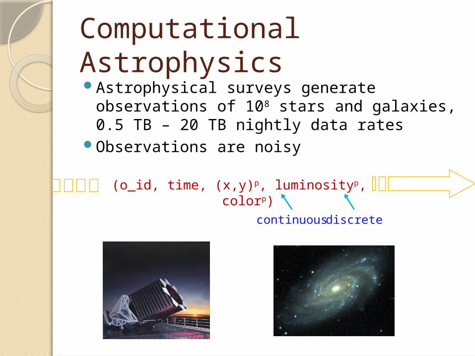
Computational AstrophysicsAstrophysical surveys generate

observations of 108 stars and galaxies, 0.5 TB – 20 TB nightly data rates

Observations are noisy

(o_id, time, (x,y)p, luminosityp, colorp)

continuous discrete

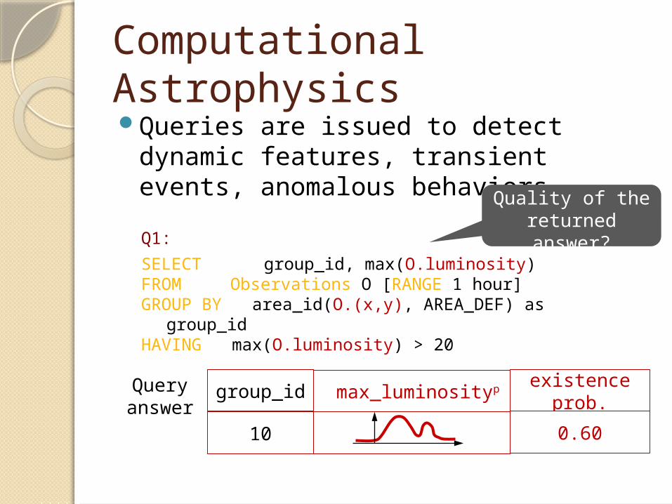
Computational AstrophysicsQueries are issued to detect dynamic

features, transient events, anomalous behaviors

Q1:

SELECT group_id, max(O.luminosity)FROM Observations O [RANGE 1 hour] GROUP BY area_id(O.(x,y), AREA_DEF) as group_idHAVING max(O.luminosity) > 20

Quality of the returned answer?

Query answer

group_id max_luminosity existence prob.

10

max_luminositypgroup_id existence prob.

0.60

RFID Tracking and MonitoringRFID technology used for object tracking and

monitoring◦ E.g., Supply chain, health care management

Raw RFID readings are noisy and incomplete

Inference yields stream with object locations

(time, tag_id, weight, (x,y)p, sizep)

continuous discrete

08:15

1 2.5kg

(10.1,12.0)

L

10:24

2 6.3kg

(2.5,3.4) M

15:30

3 1.2kg

(25.6,32.1)

S

17:42

4 3kg (13.4,26.5)

L

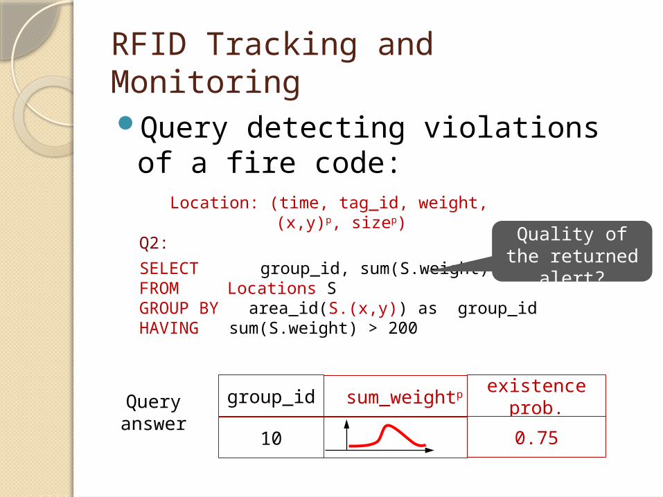
RFID Tracking and Monitoring

Query detecting violations of a fire code:Location: (time, tag_id, weight, (x,y)p, sizep)

Q2:

SELECT group_id, sum(S.weight)FROM Locations SGROUP BY area_id(S.(x,y)) as group_idHAVING sum(S.weight) > 200

Query answer

10

sum_weightpgroup_id existence prob.

0.75

Quality of the returned alert?

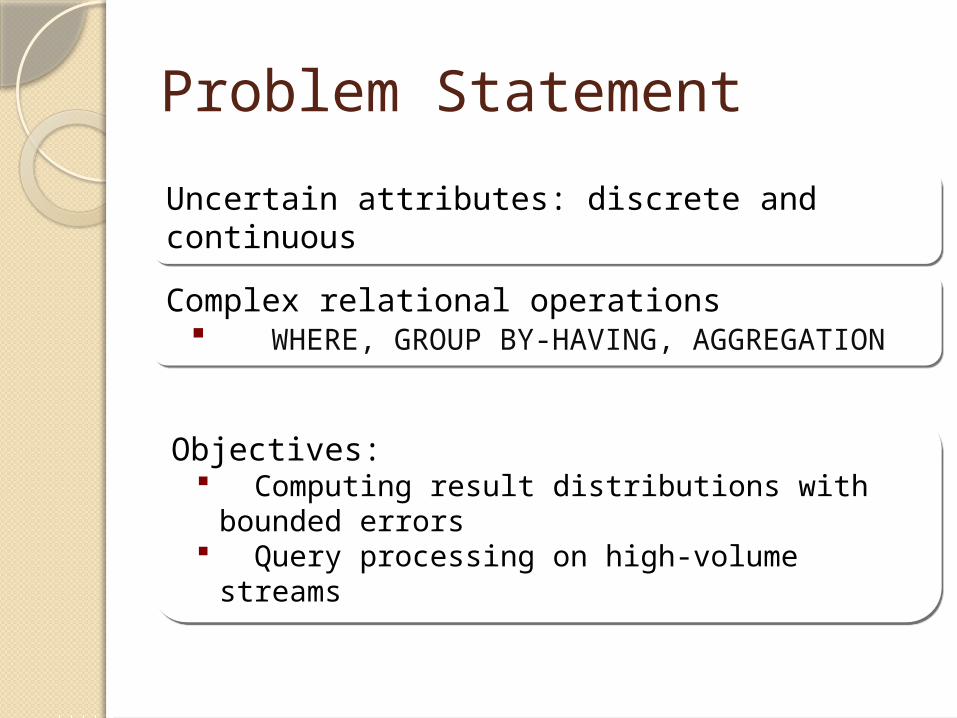
Problem Statement

Uncertain attributes: discrete and continuousUncertain attributes: discrete and continuous

Complex relational operations WHERE, GROUP BY-HAVING, AGGREGATION

Complex relational operations WHERE, GROUP BY-HAVING, AGGREGATION

Objectives: Computing result distributions with bounded

errors Query processing on high-volume streams

Objectives: Computing result distributions with bounded

errors Query processing on high-volume streams

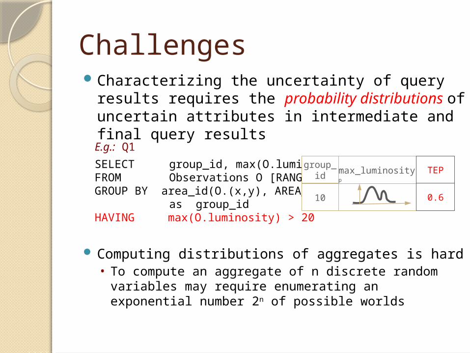
ChallengesCharacterizing the uncertainty of query

results requires the probability distributions of uncertain attributes in intermediate and final query results

Computing distributions of aggregates is hard• To compute an aggregate of n discrete random

variables may require enumerating an exponential number 2n of possible worlds

E.g.: Q1

SELECT group_id, max(O.luminosity)FROM Observations O [RANGE 1 hour] GROUP BY area_id(O.(x,y), AREA_DEF)

as group_idHAVING max(O.luminosity) > 20

10

max_luminositypgroup_id TEP

0.6

ChallengesOffering query answers with bounded errors

is crucial.◦ State-of-the-art: Monte Carlo simulation with

unbounded errors MCDB, SIGMOD’08 Handling uncertain data in array database,

ICDE’08 Database support for probabilistic attributes and

tuples, ICDE’08

In data streams, query processing needs to employ incremental computation as tuples arrive

State-of-The-Art Continuous random variables modeled by

Gaussian mixture models [SIGMOD’10] Closed-form solutions for aggregates Cannot be applied for selection, group by,

aggregates

Monte Carlo simulation gives relative approximations for evaluating HAVING predicates [Re & Suciu, VLDBJ’09]

For discrete distributions, best technique to compute sum needs O(nD3), where D is the domain size [Kanagal & Deshpande, ICDE’09]

SolutionQuery evaluation framework:

◦ Mixed-type data model◦ Approximate representations◦ Approximation metrics

Approximation algorithms for aggregates◦ Randomized algorithms: all aggregates◦ Deterministic algorithms

max, min sum, count

Query planning

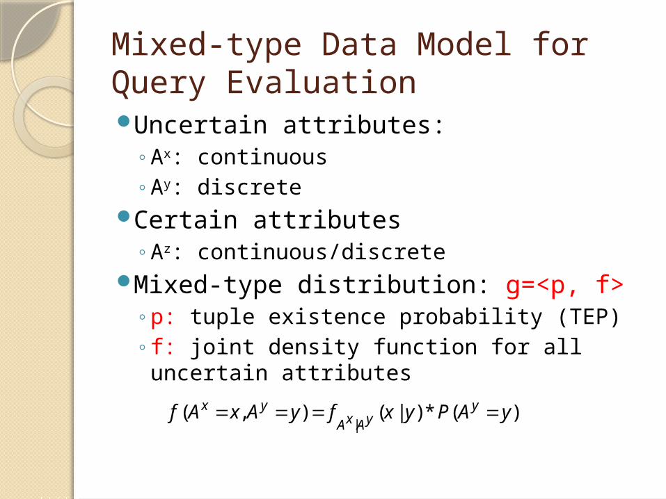
Mixed-type Data Model for Query EvaluationUncertain attributes:

◦Ax: continuous◦Ay: discrete

Certain attributes◦Az: continuous/discrete

Mixed-type distribution: g=<p, f>◦p: tuple existence probability (TEP)◦ f: joint density function for all uncertain

attributes)(*)|(),(

|yAPyxfyAxAf y

yAxA

yx

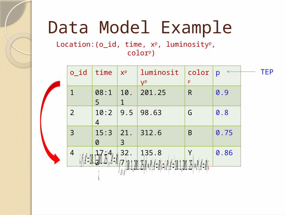
Data Model ExampleLocation:(o_id, time, xp, luminosityp, colorp)

o_id time xp luminosityp colorp p

1 08:15

10.1

201.25 R 0.9

2 10:24

9.5 98.63 G 0.8

3 15:30

21.3

312.6 B 0.75

4 17:42

32.7

135.8 Y 0.86

TEP

¿ 𝑓 ( 𝐴𝑥=(10.1,201 .25 ) , 𝐴𝑦=𝑅)¿

𝑓 𝐴𝑥∨𝐴 𝑦 (10.1,201 .25|𝑅 )∗𝑃 (𝐴𝑦=𝑅)¿=¿𝑃 (𝐴𝑥=(10.1,201 .25 ) )∗𝑃( 𝐴𝑦=𝑅)¿

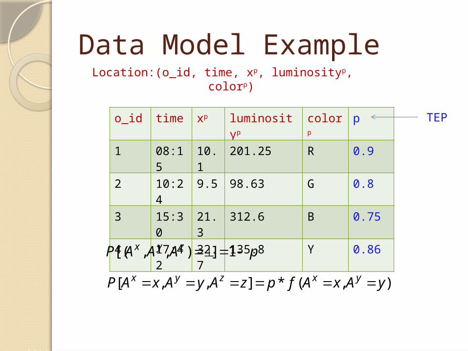
Data Model Example

pAAAP zyx 1]),,[(

),(*],,[ yAxAfpzAyAxAP yxzyx

Location:(o_id, time, xp, luminosityp, colorp)

o_id time xp luminosityp colorp p

1 08:15

10.1

201.25 R 0.9

2 10:24

9.5 98.63 G 0.8

3 15:30

21.3

312.6 B 0.75

4 17:42

32.7

135.8 Y 0.86

TEP

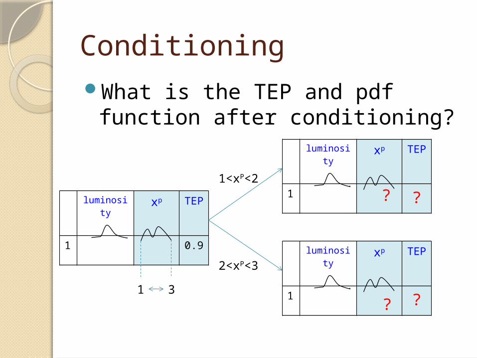
ConditioningWhat is the TEP and pdf function

after conditioning?

luminosity

xp TEP

1 0.9

luminosity

xp TEP

1 ?

luminosity

xp TEP

1 ?

1<xP<2

2<xP<3

1 3

?

?

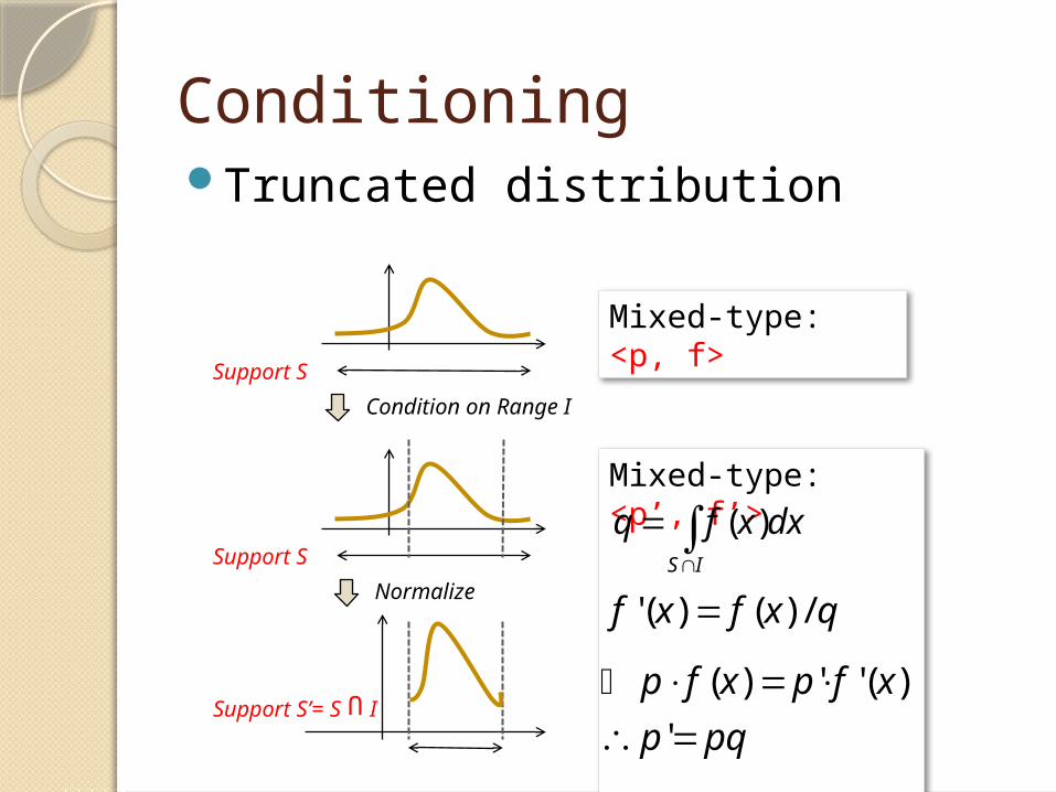
Conditioning

Mixed-type: <p, f>

Support S

Condition on Range I

Support S’= S I

U

Normalize

Support S

Mixed-type: <p’, f’>

IS

dxxfq

)(

qxfxf /)()('

pqp

xfpxfp

'

)('')(

Truncated distribution

luminosity

xp TEP

1 0.7

2 0.8

3 0.6

… … … …

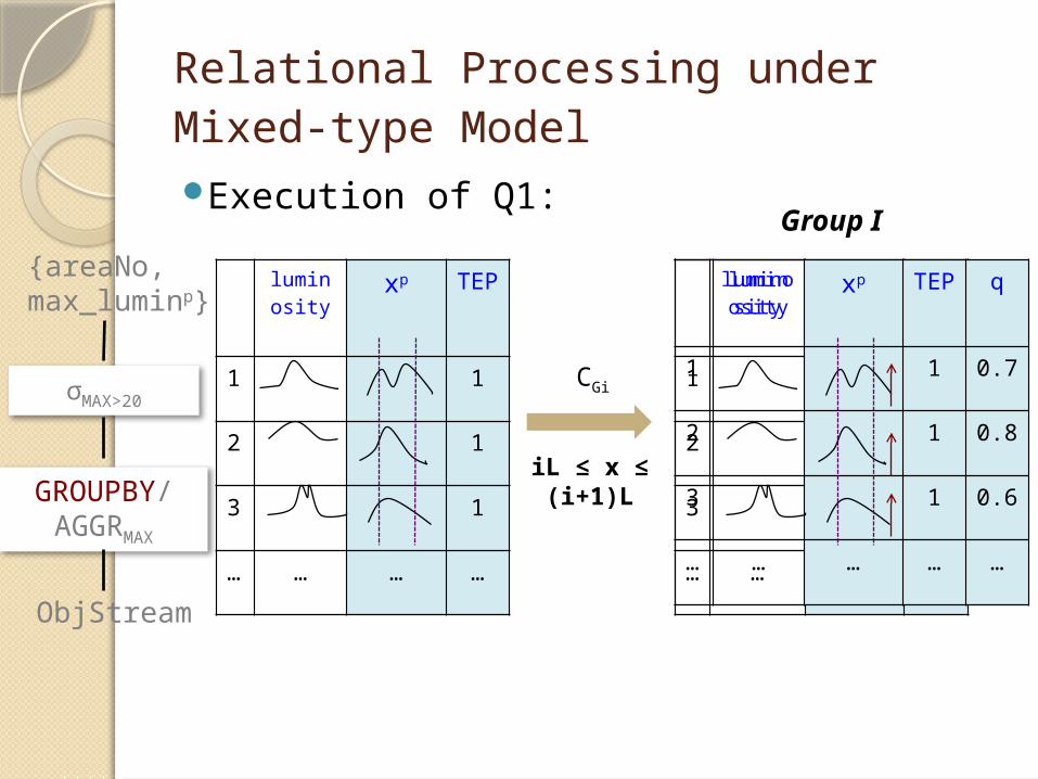
Relational Processing under Mixed-type ModelExecution of Q1:

luminosity

xp TEP

1 1

2 1

3 1

… … … …

CGi

iL ≤ x ≤ (i+1)L

Group I

luminosity

xp TEP

q

1 1 0.7

2 1 0.8

3 1 0.6

… … … … …

ObjStream

GROUPBY/AGGRMAX

σMAX>20

{areaNo, max_luminp}

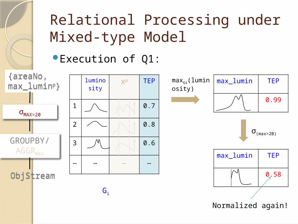
Relational Processing under Mixed-type Model

maxGi(luminosity)

max_lumin TEP

0.99

σ(max>20)

max_lumin TEP

0.58

luminosity

xp TEP

1 0.7

2 0.8

3 0.6

… … … …

Execution of Q1:

ObjStream

GROUPBY/AGGRMAX

σMAX>20

{areaNo, max_luminp}

ObjStream

GROUPBY/AGGRMAX

σMAX>20

{areaNo, max_luminp}

Gi

Normalized again!

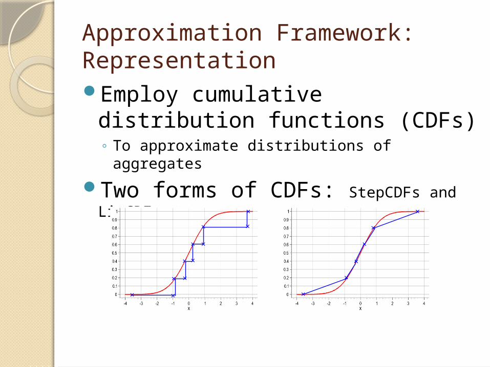
Approximation Framework: RepresentationEmploy cumulative distribution

functions (CDFs) ◦ To approximate distributions of aggregates

Two forms of CDFs: StepCDFs and LinCDFs

×

×

×

×

×

××

××

××

××

××

××

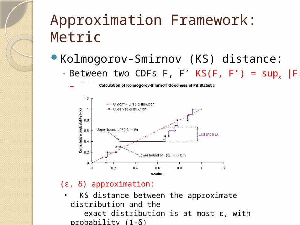
Approximation Framework: MetricKolmogorov-Smirnov (KS) distance:

◦ Between two CDFs F, F’ KS(F, F’) = supx |F(x) – F’(x)|

(ε, δ) approximation:

• KS distance between the approximate distribution and the exact distribution is at most ε, with probability (1-δ)

• δ=0: deterministic, δ>0: randomized

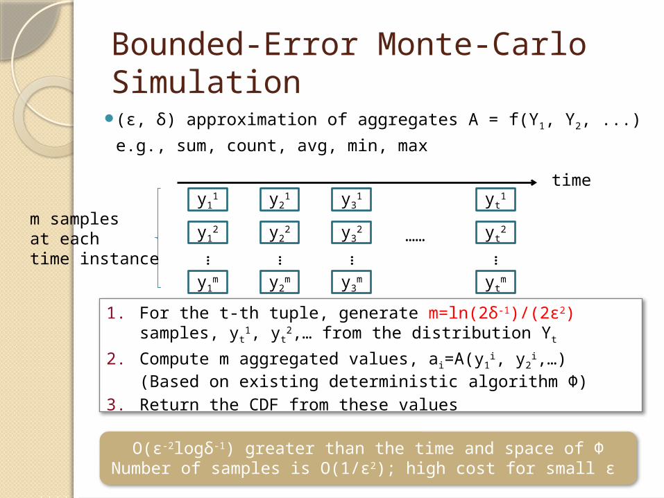
Bounded-Error Monte-Carlo Simulation(ε, δ) approximation of aggregates A = f(Y1, Y2, ...)

e.g., sum, count, avg, min, max

1. For the t-th tuple, generate m=ln(2δ-1)/(2ε2) samples, yt1,

yt2,… from the distribution Yt

2. Compute m aggregated values, ai=A(y1i, y2

i,…) (Based on existing deterministic algorithm Φ)

3. Return the CDF from these values

O(ε-2logδ-1) greater than the time and space of ΦNumber of samples is O(1/ε2); high cost for small ε

y11

…

y12

y1m

y21

…

y22

y2m

y31

…

y32

y3m

yt1

…

yt2

ytm

……

time

m samples at each time instance

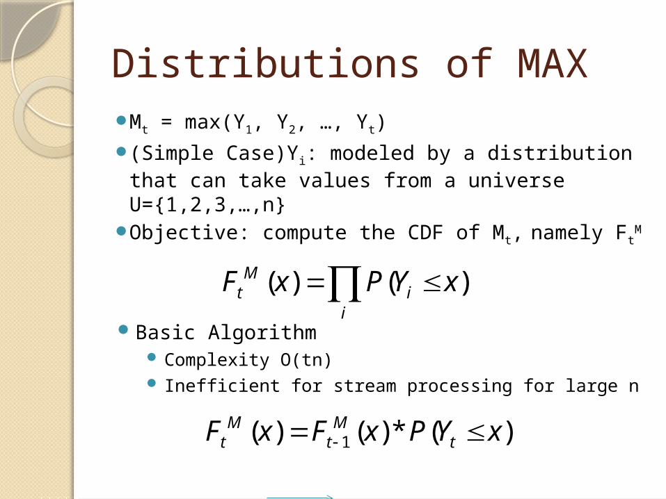
Distributions of MAXMt = max(Y1, Y2, …, Yt)(Simple Case)Yi: modeled by a distribution

that can take values from a universe U={1,2,3,…,n}

Objective: compute the CDF of Mt, namely FtM

i

iMt xYPxF )()(

Basic Algorithm Complexity O(tn) Inefficient for stream processing for large n

)(*)()( 1 xYPxFxF tMt

Mt

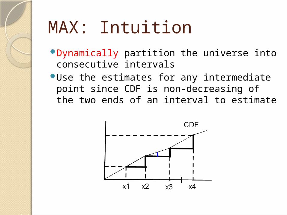
MAX: IntuitionDynamically partition the universe into

consecutive intervalsUse the estimates for any intermediate

point since CDF is non-decreasing of the two ends of an interval to estimate

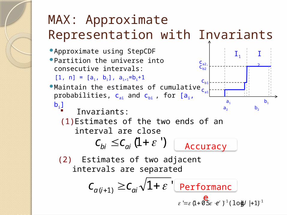
MAX: Approximate Representation with Invariants Approximate using StepCDF Partition the universe into

consecutive intervals: [1, n] = [ai, bi], ai+1=bi+1

Maintain the estimates of cumulative probabilities, cai and cbi , for [ai, bi]

I1 I2

a1 b1 a2

b2

ca1

cb1

cb2

ca2,

Invariants:(1) Estimates of the two ends of an interval

are close

(2) Estimates of two adjacent intervals are separated

Accuracy

Performance

)'1( aibi cc

'1)1( aiia cc11 )1||(log)5.01(' Ue

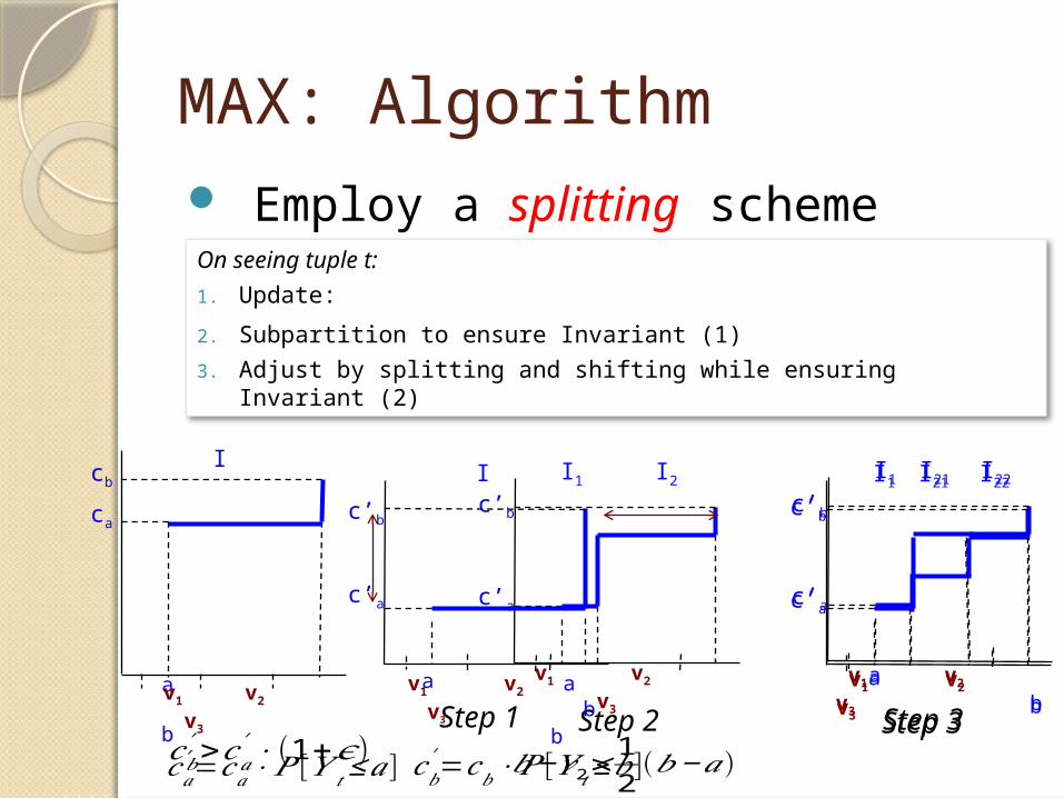
MAX: Algorithm Employ a splitting schemeOn seeing tuple t:

1. Update:

2. Subpartition to ensure Invariant (1)

3. Adjust by splitting and shifting while ensuring Invariant (2)

v1 v2 v3 a b

I1

c’a

c’b

I2

Step 2a b

I

ca

cb

v1 v2 v3

I

a b

c’a

c’b

v1 v2 v3

Step 1

I1

c’a

c’b

I22I21

Step 3

a b

v1 v2 v3 v1 v2 v3a b

I1

c’a

c’b

I22I21

Step 3

𝑐𝑎′ =𝑐𝑎 ⋅ 𝑃 [𝑌 𝑡≤𝑎 ]𝑐𝑏

′ =𝑐𝑏⋅ 𝑃 [𝑌 𝑡≤𝑏]𝑐𝑏′ >𝑐𝑎

′ ⋅(1+𝜖 ) 𝑏−𝑣2>12(𝑏−𝑎)

MAX: AlgorithmAt any step in the algorithm, the

number of intervals is bounded as follows:

The maximum generation of an interval is

MAX: Analysis

2. Number of intervals is bounded

3. Number of times an interval is split is bounded, i.e., logU

(ε, 0) algorithm for max, update time is O(ε-1 logU lnε-1 )

1. Estimates of the two ends of an interval are bounded Estimates of any point in an interval are bounded

Extend to continuous distributions:A general approach is to consider a large universe of size 264. The complexity is then proportional to log 264 =64.

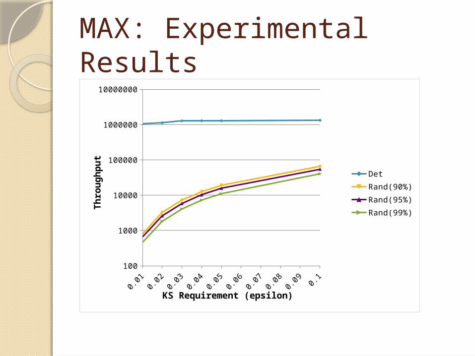
MAX: Experimental Results

0.01 0.02 0.03 0.04 0.05 0.06 0.07 0.08 0.09 0.1100

1000

10000

100000

1000000

10000000

Det

Rand(90%)

Rand(95%)

Rand(99%)

KS Requirement (epsilon)

Th

rou

gh

pu

t

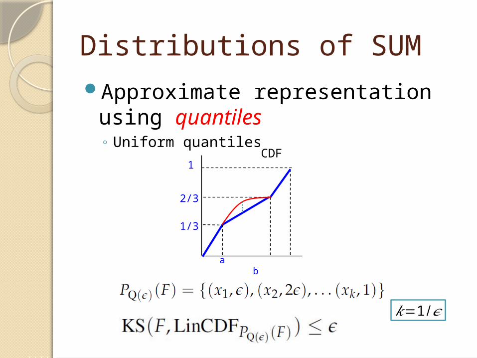
Distributions of SUMApproximate representation

using quantiles◦ Uniform quantiles

CDF

a b

2/3

1

1/3

𝑘=1 /𝜖

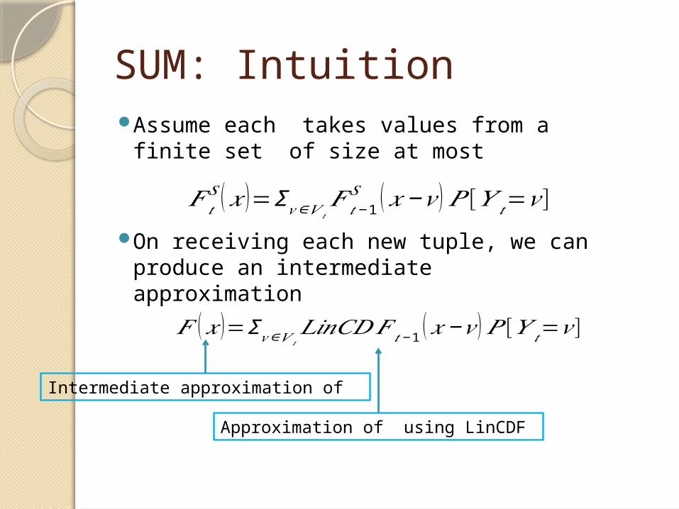
SUM: IntuitionAssume each takes values from a finite

set of size at most

On receiving each new tuple, we can produce an intermediate approximation

𝐹 𝑡𝑆 (𝑥 )=Σ𝑣∈𝑉 𝑡

𝐹 𝑡−1𝑆 (𝑥−𝑣 ) 𝑃 [𝑌 𝑡=𝑣 ]

𝐹 (𝑥 )=Σ𝑣∈𝑉 𝑡𝐿𝑖𝑛𝐶𝐷𝐹 𝑡− 1 (𝑥−𝑣 )𝑃 [𝑌 𝑡=𝑣 ]

Approximation of using LinCDF

Intermediate approximation of

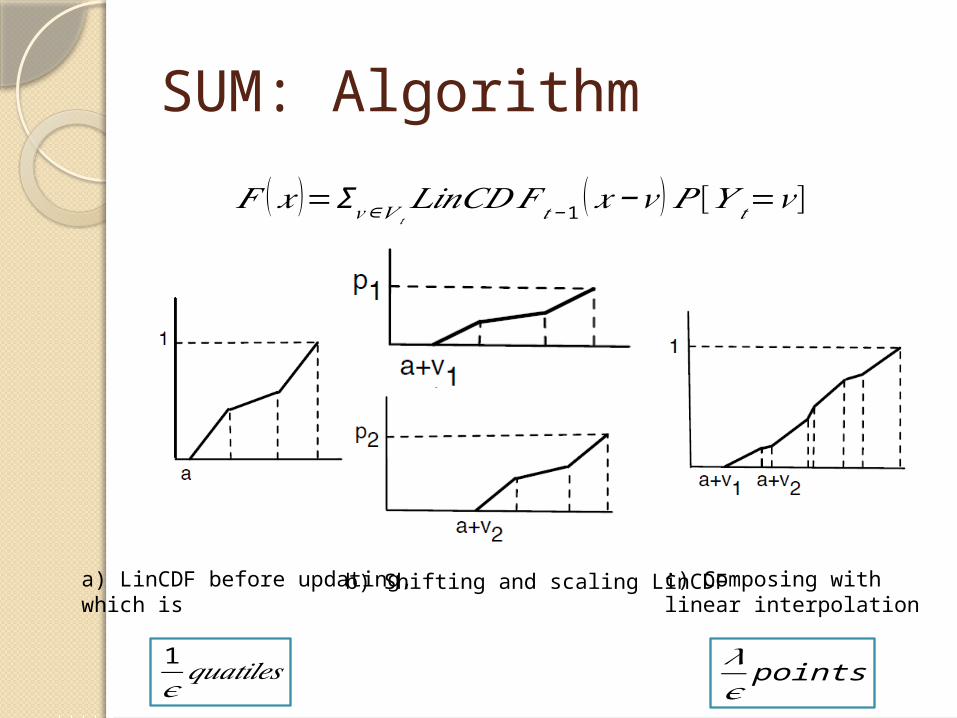
SUM: Algorithm

𝐹 (𝑥 )=Σ𝑣∈𝑉 𝑡𝐿𝑖𝑛𝐶𝐷𝐹 𝑡− 1 (𝑥−𝑣 )𝑃 [𝑌 𝑡=𝑣 ]

b) Shifting and scaling LinCDFa) LinCDF before updating,which is

1𝜖𝑞𝑢𝑎𝑡𝑖𝑙𝑒𝑠

c) Composing with linear interpolation

𝜆𝜖points

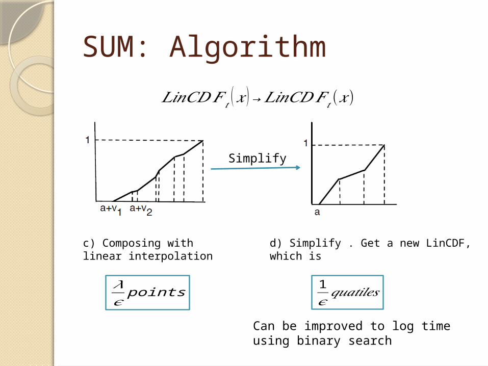
SUM: Algorithm

c) Composing with linear interpolation

d) Simplify . Get a new LinCDF,which is

1𝜖𝑞𝑢𝑎𝑡𝑖𝑙𝑒𝑠

𝜆𝜖points

Simplify

𝐿𝑖𝑛𝐶𝐷𝐹 𝑡 (𝑥 )→𝐿𝑖𝑛𝐶𝐷𝐹𝑡 (𝑥)

Can be improved to log timeusing binary search

SUM: Analysis(ε, 0) algorithm for sum

◦Space ◦Update time

Supporting continuous distributions◦Discretize input distribution by

LinCDF or StepCDF◦Total error is the sum of

discretization error and approximation error

SUM: Experimental Results

0.01 0.02 0.03 0.04 0.05 0.06 0.07 0.08 0.09 0.1100

1000

10000

100000

DetRand(90%)Rand(95%)Rand(99%)

KS Requirement (epsilon)

Th

rou

gh

pu

t

Approximate Query AnswersExtended KS distance, named KSM

KSM(G, G’) = max(|p – p’|, supx |p F(x) – p’ F’(x)|,

supx|p (1 – F(x)) – p’ (1 – F’(x))|)Bound quantities such as , and

Query approximation objective: For query answer set and exact answer set ◦ and should have the same number of tuples◦ The corresponding attribute in the

corresponding tuple in is at most with prob. 1-

Approximate Query AnswersConsider Select-From-Where-Groupby-Having block◦ One aggregate predicate in the Having clause

Selection/Group By

Aggregation

Selection/Projection

ε = 0

ε > 010

max_luminositypgid TEP

0.6ε

Error occurs here!

Query PlanningPlanning: find a query plan that meets the

objective

Proposition on Selection: Selection on an attribute with (ε, δ) –approx, using a range condition is (2ε, δ) If the selection uses a union of ranges, the approximation

error is twice the sum, i.e., 2εi.

Top-down approach to provision error bounds◦ If the error is ε, we should provision ε/2 for the

approximation of sum

Query Planning: Experimental Results

0.01 0.03 0.05 0.07 0.090

1000

2000

3000

4000

5000

6000

7000

DetRand(90%)Rand(95%)Rand(99%)

KS Requirement (epsilon)

Th

rou

gh

pu

t

Query Planning: Experimental Results

ConclusionEvaluation framework and approximation

techniques for complex operations◦ Randomized algorithms: general◦ Deterministic algorithms: often better◦ For complex queries, the errors are bounded

while having throughput of thousands of tuples per sec

Future work◦ Wider range of aggregates◦ Correlation among derived attributes◦ Query optimization

DiscussionError bound of SUM

Assumption on Vt

𝐾𝑆 (𝐹 ,𝐿𝑖𝑛𝐶𝐷 𝐹𝑡 )≤𝜖

𝐾𝑆 (𝐹𝑡𝑆 ,𝐿𝑖𝑛𝐶𝐷𝐹𝑡 )≤ 𝑡 𝜖

Thanks!