Journal of Computational and Applied Mathematics 12&13 (1985) 491-503 North-Holland

491

Condition of boundary integral equations arising from flow computations

H. NIESSNER and M. RIBAUT BBC Brown Boueri & Co, Ltd., CH-5401 Baden, Switzerland

Received 23 May 1984 Revised 12 November 1984

Abstract: Stating flow boundary conditions for normal and tangential velocities leads to Fredholm integral equations of the first and second kind. Approximating the vortex distribution on pressure and suction side by piecewise linear functions with equidistant knots, collocation yields a commonly overdetermined system of linear equations with the vortex densities as unknowns. There are several possibilities for collocation. The question arises what kind of integral equation and what collocation points are to be preferred. Our main conclusions based on condition numbers of the resulting linear systems are: -The equation of the first kind with Cauchy singular kernel does not appear to be worse conditioned than the equation of the second kind with regular kernel. - Collocation points for the equation of the first kind are better placed in between the knots, for the equation of the second kind at the knots. - The circulation is mainly determined by the equation of the first kind, the mean velocity level by the equation of the second kind. Employing simultaneously equations of the first and second kind generally improves the solution and allows to cope with aerodynamic profiles of any thickness and loading.

Keywords: Boundary integral equations, collocation, condition numbers, flow computations.

AMS(M0S) Subject Classificahon: 65RO5, 76-04

1. Flow computations by boundary integral methods

Efficient computation of potential flow is rendered possible by the method of singularities. In the more satisfying variants the flow field is constructed from a continuous distribution of sources [6], dipoles [5] or vortices on the boundary. The flow boundary condition then yields a Fredholm integral equation for the unknown singularity distribution. The solution needs to be computed on the boundary only, thus reducing the dimension of the problem by one. Therefore the method is also called boundary integral [2] or boundary element method, the latter since the unknown distribution is commonly approximated by a linear combination of functions with local support. Its advantage over finite difference or finite element methods with comparable discreti- sation length stems from its accuracy rather than from lower computation time, despite the lower dimension. The resulting system of linear equations is not sparse and the evaluation of its coefficients is costly [2].

Vortices are the only physically meaningful singularities on solid flow boundaries. By allowing part of them to be on a sheet within the flow field even boundary layer effects can be simulated.

0377-0427/85/%3.30 0 1985, Elsevier Science Publishers B.V. (North-Holland)

492 H. Niessner, M. Ribaut / BoundaT integral equations

In a more sophisticated form the method successfully provides solutions for subsonic and shock-free transonic weakly viscous flows through the rotating cascades of a turbomachine [13]. In principle the boundary conditions of two dimensional flow can be formulated for the vector potential or the stream function like in [4], which leads to a Fredholm integral equation of the first kind with logarithmic kernel. Physically more satisfying is to state the boundary conditions directly for the velocity in normal or tangential direction yielding a Fredholm integral equation of the first or second kind. Should one use that of the first kind or that of the second kind or both simultaneously?

Because of the regular kernel some authors use the equation of the second kind (e.g. [lo]). It is generally supposed that this works only with profiles having continuous curvature and sufficient thickness. Therefore other workers prefer the equation of the first kind (e.g. [7]) with Cauchy singular kernel, whereby the system of linear equations resulting from discretization is sometimes stabilized by using more linear equations than unknowns.

Approximating the vortex distribution on pressure and suction side by piecewise linear functions with equidistant knots, collocation yields a commonly overdetermined system of linear equations with the vortex densities at the knots as unknowns. Are the collocation points better placed at the knots or in between them?

Recently much work has been done to answer the above questions in a highly general and abstract rigorous form. According to [16] the following properties hold with piecewise linear trial functions: - Collocation at the knots is sufficient [1,11] and necessary [15] for optimal order convergence in the case of Fredholm integral equations of the second kind, since they belong to the class of strongly elliptic boundary integral equations. - Collocation at the midpoints in between the knots is sufficient and necessary [15] for optimal order convergence in the case of Fredholm integral equations of the first kind with Cauchy kernel.

Interestingly enough it seems that this is true for smoothest splines of any odd degree [1,15], whereas for even degree the inverse holds, i.e. collocation is optimal at the midpoints for strongly elliptic equations [14,15], at the knots for equations of the first kind with Cauchy kernel [15].

Our much simpler investigation based on the condition of the generated system of linear equations is aimed at the more practical problems of flow calculation. To this end we consider the flow past a cicular cylinder and a flat plate as an analytical model. Furthermore we present numerical experiments with a number of airfoil and cascade flows. The results are in good agreement with theory.

2. The basic form of the integral equations

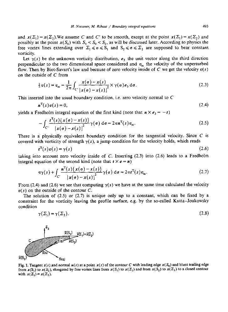
For the sake of illustrating the basic properties of the method let us consider the two-dimen- sional plane flow around an airfoil with the contour C represented by x = x(s) with tangent t = Z(S) and normal n = n(s) oriented as in Fig. 1, where s is the arc length on C with

S,dS<S,. (2.1)

As indicated in Fig. 1, C may eventually not be closed but instead be elongated to a closed contour C’ by free vortex lines, where C’ is represented by x = x(a) with

&<UbZ, (2.2)

H. Niessner, hi. Ribaut / Boundary integral equations 493

and x(X:,) = x(Z:,).We assume C and C’ to be smooth, except at the point x(2:,) = ~(2~) and possibly at the point x( SO) with S, < SO < S,, as will be discussed later. According to physics the free vortex lines extending over & ( (I < S, and S, G o 6 .‘Zc, are supposed to bear constant vorticity.

Let y(s) be the unknown vorticity distribution, e3 the unit vector along the third direction perpendicular to the two dimensional space considered and u, the velocity of the unperturbed flow. Then by Biot-Savart’s law and because of zero velocity inside of C we get the velocity n(s) on the outside of C from

(2.3)

This inserted into the usual boundary condition, i.e. zero velocity normal to C

nT(.+(.r) = 0,

yields a Fredholm integral equation of the first kind (note that n X e3 = -i)

(2 -4)

_ J ‘T(s){+) -x(s)) y(u) da = 2,.+)u

=’ Ix(u) -x(s)j2 co* (2.5)

There is a. physically equivalent boundary condition for the tangential velocity. Since C is covered with vorticity of strength y(s), a jump condition for the velocity holds, which reads

tT(+(s> = Y(S) (2.6)

taking into account zero velocity inside of C. Inserting (2.3) into (2.6) leads to a Fredholm integral equation of the second kind (note that t X e = n)

nT(S){ x(u) - x(s)) y(u) da =

Ix(u>-x(s))2 2,,.$(s)u

co* (2.7)

From (2.4) and (2.6) we see that computing y(s) we have at the same time calculated the velocity u(s) on the outside of the contour C.

The solution of (2.5) or (2.7) is unique only up to a constant, which can be fixed by a constraint for the vorticity leaving the profile surface, e.g. by the so-called Kutta-Joukowsky condition

Y(&) = Y(~z>* (2.8)

Fig. 1. Tangent t(s) and normal n(s) at a point x(s) of the contour C with leading edge x(S,,) and blunt trailing edge from x(S1) to x( S,), elongated by free vortex lines from x( S,) to x(&) and from x( S,) to x(2,) to a closed contour with x(2:,) = x(X,).

494 H. Niessner, M. Ribaut / Boundary integral equations

Inserting the Taylor series of x(a) around x(s) truncated after the first order term into (2.5) and (2.7) we see that the kernel of (2.5) is Cauchy singular at u = s (i.e. the singularity is of the form

I/(0 - s)), whereas (2.7) is regular.

3. The numerical method of solution

We approximate the unknown vorticity distribution y(a) by a piecewise linear function with knots s, satisfying

s*=sg<sl<s*< -** <s,=s,,

expressing it as a linear combination

Y(O) = i Y”UJ) v=o

of hat-functions

(3-I)

(3.2)

where we use the symbol

(3.4)

The coefficients y, in (3.2) are the vortex densities at the knots s,. Formally defining

s-1= -co and s,,+r = +co, (3.5)

we get Ba(u) = 1 for u < sO and B,,(u) = 1 for u > s, and (3.2) remains constant on the free vortex lines, as required from physics.

Inserting (3.2) into (2.5) or (2.7) we obtain one linear equation in the (n + 1) unknown vortex densities y, for every collocation point. The integrals occuring in the coefficients may be computed by some suitable quadrature rule which does not concern us here. An additional equation is provided by the Kutta-Joukowsky condition (2.8). Therefore we need at least n equations from collocation. As collocation points we consider the (n + 1) knots

so, Sl,...,S” (3.6)

or the n midpoints in between

s1/2, s3/2,*m*, &-1/2~ (3.7)

where

Sv+l/Z = i(sv + S”,l) (3-g)

The case of more equations than unknowns, as it occurs with the collocation points (3.6), we cope easily with by solving the collocation equations in the least squares sense the Kutta-Joukowsky condition being a constraint. Several proposals for handling such problems are found in [9]. Besides direct substitution of the constraint, the following procedure is simple and efficient: impose a high weight onto the constraint and solve all equations in the least squares sense by Householder transformations.

If. Niessner, M. Ribaut / Boundary integral equations 495

As condition number of an overdetermined system of linear equations in n’ unknowns we use the ratio of the largest to the smallest of the n’ largest singular values. Foregoing we eliminate existing constraints by modifying the coefficient matrix corresponding to a projection of the solution into the null space of the constraints (see [9]).

4. Actual choice of knots and collocation points

The contour of aerodynamic profiles generally shows one region of large curvature. There we select a point x( S,) (see Fig. l), which we call the leading edge. It is sharp or smooth depending on whether the curvature is infinitely large or not. The points x( St) and x(&) represent the trailing edge. It may be smooth, blunt with free vortex lines (as in Fig. l), or sharp. The leading edge divides the contour into the suction side with

S, G s < S, (4.1)

and the pressure side with

s,<s<s,. (4.2)

We divide pressure and suction side into an equal number in of equidistant intervals (we suppose n to be even), the boundaries of which are the knots. Thus we obtain, e.g.

so = s,, %/2= 0, s s, = s, .

The best result we can expect from our calculation is a good approximation in some sense of the exact solution. This is facilitated on a sharp leading edge in particular by permitting there a discontinuity. For this purpose we may consider s,,~ a double knot or equivalently divide the hat-function Bn,2( a) into two parts

4,2b) = e-,2(4 +$2(u), (4.4) the first one being nonzero for u -C s,,,~ only, the second one for u >, s,,,~ only. Then the term y,,,,&,,(a) in (3.2) has to be replaced by

vn-,2 472 ( CJ > + x+,2 q,2 ( 0 ) 7 (4.5)

increasing the number of unknowns by one. On the other hand with a smooth trailing edge the number of unknowns is one less because of continuity (y. = y,).

The feasibility of corner points on the contour is discussed in [3] and [12]. At such points equation (2.3) is not valid, tangent and normal vectors are not unique, and a nonintegrable singularity appears in the integrand of the coefficient belonging to the vortex density at that point. Therefore we exclude sharp edges from collocation. From the two sets of collocation points (3.6) and (3.7), only (3.6) is affected by this restriction.

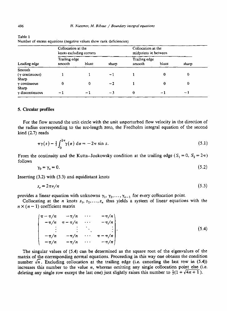
By the above rules we obtain Table 1, giving the number of excess equations using integral equations of first or second kind only (negative values show rank deficiency). The larger the number of excess equations, the better are the condition numbers one can expect for the system of equations. From this point of view the collocation points in between the knots seem to be preferable.

496 H. Niessner, M. Ribaut / Boundary integral equations

Table 1 Number of excess equations (negative values show rank deficiencies)

Collocation at the Collocation at the knots excluding comers midpoints in between

Leading edge

Smooth ( y continuous) Sharp y continuous

Sharp y discontinuous

Trailing edge Trailing edge smooth blunt sharp smooth blunt sharp

1 1 -1 1 0 0

0 0 -2 1 0 0

-1 -1 -3 0 -1 -1

5. Circular profiles

For the flow around the unit circle with the unit unperturbed flow velocity in the direction of the radius corresponding to the arc-length zero, the Fredholm integral equation of the second kind (2.7) reads

ay(s) - $/u’;(o) da = -2a sin s. (5.1)

From the continuity and the Kutta-Joukowsky condition at the trailing edge (S, = 0, S, = 2a) follows

yo=y,=o. (5.2)

Inserting (3.2) with (3.3) and equidistant knots

s, = 27rv/n (5.3)

provides a linear equation with unknowns yl, y2, . . . , yn _ 1 for every collocation point. Collocating at the n knots sl, s2,. . ., s,, thus yields a system of linear equations with the

n X (n - 1) coefficient matrix

The singular values of (5.4) can be determined as the square root of the eigenvalues of the matrix of the corresponding normal equations. Proceeding in this way one obtains the condition number fi. Excluding collocation at the trailing edge (i.e. canceling the last row in (5.4)) increases this number to the value n, whereas omitting any single collocation point else (i.e. deleting any single row except the last one) just slightly raises this number to $(l + {m).

H. Niessner, M. Ribauf / Boundary integral equations 497

Collocation at the n midpoints ~i,~, s~,~, . . . , s,_ ,,y2 leads to the n X (n - 1) coefficient matrix

/ T/2 - n/n -q/n e-0 -n/n’

n/2 - 7r/n ~/2 - 71/n . . . - n/n

- T/n T/2-n/n *. . . 65)

. . n/2 - 7r/n

\ - 71/n -T/n mm. q/2 - 7r/n,

Since the homogeneous system has the non-trivial solution (1, 0, 1, 0,. . . , l), this matrix is singular for even n (for odd n the condition number is at about n). So collocation at the knots is more favourable with equations of the second kind.

The Fredholm integral equation of the first kind (2.5) corresponding to (5.1) reads

-; J 2n u-s

cot - 2 y(o) da = 2Tcos s 0

(5.6)

Including the coefficients for the unknown y,, = y. collocation at the knots yields an n X n

matrix, which is singular because without condition (5.2) the solution is determined only up to a constant. This matrix is skew-symmetric, and since eigenvalues appear in conjugate pairs it has rank deficiency of at least 2 for even n, so that substituting (5.2) the system remains singular (for odd n the condition number is again at about n). Equation (5.6) collocated at the knots is a famous example in [g]. Numerical evidence indicates however a condition number of s 1.176 while collocating at the midpoints (3.7). This is very little worse than the condition number resulting from the equation of the second kind collocated at the knots.

6. Smooth profiles

From a physical point of view one would expect the linear equations to be ill-conditioned if a variation of the unknown y, at a knot s, close to a collocation point s has a small effect only on the right hand side of the equation, i.e. if the coefficient a,(s) of y, in this equation is small.

In fact, assuming a smooth profile and equidistant collocation points and replacing x(a) in (2.5) and (2.7) by a truncated Taylor series around the collocation point, we approximately obtain the coefficients for 0 < v < n

a(l) z () Y

and

aS’)(s,*,,,) = f; log 3,

generated by the equations of the first kind (2.5) as well as

a(2) z .lr Y

and

a:*%% * i/2 ) = $71

generated by the equations of the second kind (2.7).

(6.1)

(6 -2)

(6.3)

(6.4)

498 H. Niessner, M. Ribaut / Bounday integral equations

Table 2 Results for VKI-LS 59 cascade with n = 48.

Condition number Average velocity error in % Error of the computed circulation in %

Fredholm integral equations of the first kind

at the in knots between

68 32

3 0.5

0.1 0.1

Fredholm integral equations of the second kind

at the in knots between

38 120

2 3.5

3.1 0.4

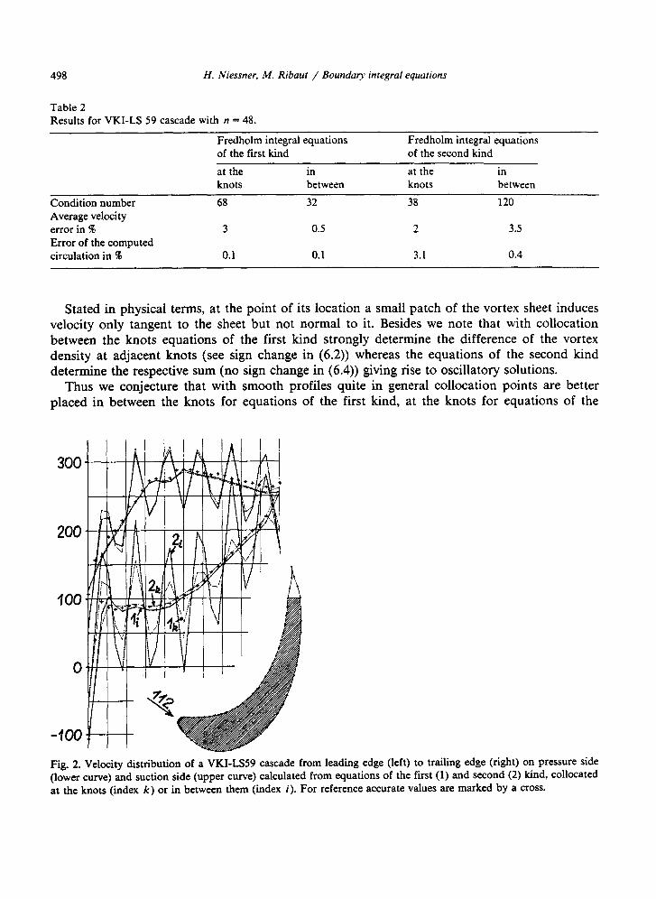
Stated in physical terms, at the point of its location a small patch of the vortex sheet induces velocity only tangent to the sheet but not normal to it. Besides we note that with collocation between the knots equations of the first kind strongly determine the difference of the vortex density at adjacent knots (see sign change in (6.2)) whereas the equations of the second kind determine the respective sum (no sign change in (6.4)) giving rise to oscillatory solutions.

Thus we conjecture that with smooth profiles quite in general collocation points are better placed in between the knots for equations of the first kind, at the knots for equations of the

Fig. 2. Velocity distribution of a VKI-LS59 cascade from leading edge (left) to trailing edge (right) on pressure side (lower curve) and suction side (upper curve) calculated from equations of the first (1) and second (2) kind, collocated at the knots (index k) or in between them (index i). For reference accurate values are marked by a cross.

H. Niessner, M. Ribaut / Boundary integral equations 499

second kind. This is supported by the results of calculations with n = 48 on the VKI-LS 59 cascade in Table 2.

We observe that the most accurate result is obtained with equations of the first kind collocated at the midpoints in between the knots. In order to make the effects more visible, the computed velocity distributions in Fig. 2 (likewise in Figs. 3 and 4) are shown for n = 24.

7. Flat plates

For a flat plate of length say 1 with S, = - 1, S,, = 0, S, = + 1, a unit unperturbed flow velocity with an angle a to the direction of the plate and thickness converging to zero the equation of the second kind (2.7) becomes

n{y(+JsI)-y(-/sI)}=2acoscr. (7.1) This determines solely the difference of the vortex strengths on pressure and suction side,

which because of (2.6) is the mean of the velocity on both sides

u(l.q)= t{Y(+l+YH4)1~ U-2) It leaves open the sum of the vortex strengths on both sides. Therefore the system of linear equations obtained by substituting (3.2) and (2.8) into (7.1) is singular.

With the same assumptions the equation of the first kind (2.5) obtains the form

I 1~(~u)~~(~u)du~2n~i~a 0

which solely determines the sum of the vortex strenghts on pressure and suction side and therefore the circulation

r=jol{y(-o)+y(+o)}de. (7.4)

This time the difference of the vortex strengths on both sides is left open. Substituting (3.2) and (2.8) into (7.3) again yields a singular system of linear equations.

However a regular system of linear equations may be obtained using equations of the first and second kind simultaneously. It remains to clarify which collocation points are to be preferred. Since with the flat plate the collocation points at leading and trailing edge are excluded, collocation in between the knots seems to offer more advantage.

8. Thin profiles

Obviously for any thin profile the equations of the first kind mainly determine the circulation, whereas the equations of the second kind determine the mean velocity. Such a tendency is already found in Table 2, where the error of the circulation calculated via the solution of the Fredholm integral equation of the first kind is essentially smaller than that obtained from the equation of the second kind.

With thin profiles the linear equations resulting from the Fredholm integral equation of the first or second kind alone tend to be ill-conditioned. Nevertheless, circulation-free flow may well

500 H. Niessner, M. Ribaut / Boundar): integral equations

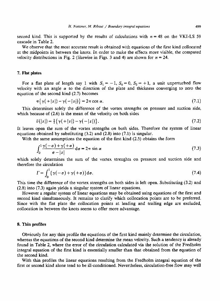
Fig. 3. Velocity distribution of NACA 0012 airfoil with zero angle of attack (i.e. circulation free flow), representation

and symbols as in Fig. 2.

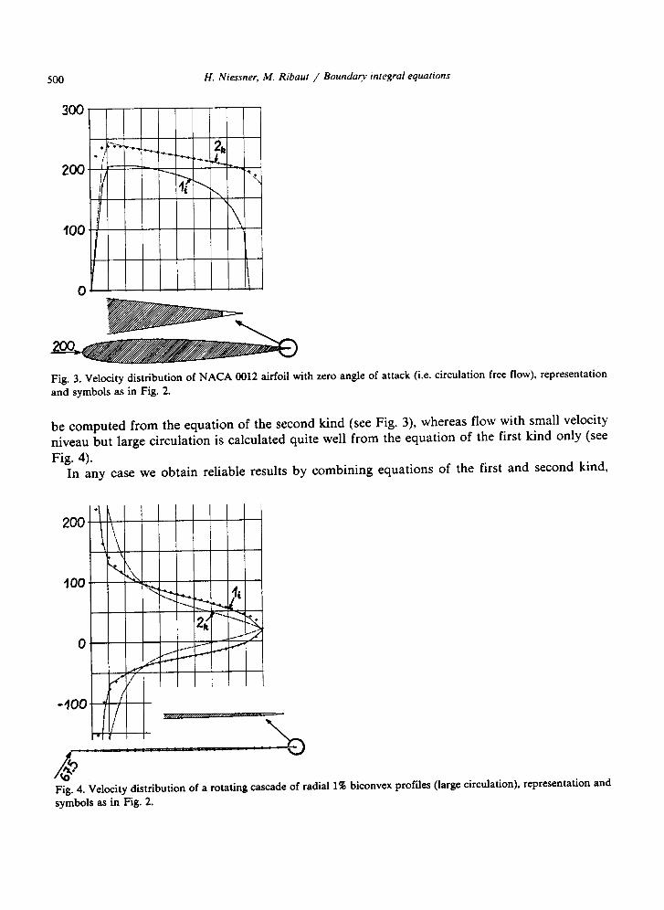
be computed from the equation of the second kind (see Fig. 3), whereas flow with small velocity niveau but large circulation is calculated quite well from the equation of the first kind only (see Fig. 4).

In any case we obtain reliable results by combining equations of the first and second kind,

200

100

0 /

-100

/ J? Fig. 4. Velocity distribution of a rotating cascade of radial symbols as in Fig. 2.

1% biconvex profiles (large circulation), representation and

H. Niessner, hi. Ribaut / Boundaty integral equations 501

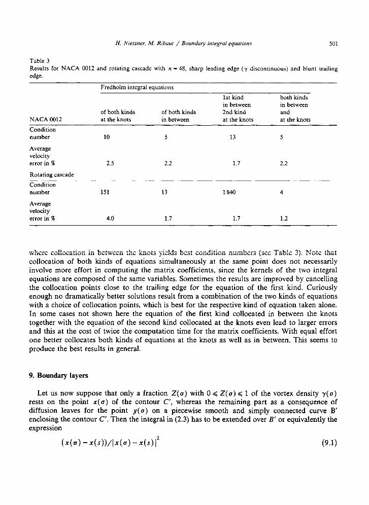
Table 3 Results for NACA 0012 and rotating cascade with n = 48, sharp leading edge (y discontinuous) and blunt trailing edge.

Fredholm integral equations

NACA 0012 of both kinds at the knots

of both kinds in between

1st kind in between 2nd kind at the knots

both kinds in between

and at the knots

Condition number

Average velocity error in %

Rotating cascade

Condition number

Average velocity

error in %

10 5 13 5

2.5 2.2 1.7 2.2

151 13 1840 4

4.0 1.7 1.7 1.2

where collocation in between the knots yields best condition numbers (see Table 3). Note that collocation of both kinds of equations simultaneously at the same point does not necessarily involve more effort in computing the matrix coefficients, since the kernels of the two integral equations are composed of the same variables. Sometimes the results are improved by cancelling the collocation points close to the trailing edge for the equation of the first kind. Curiously enough no dramatically better solutions result from a combination of the two kinds of equations with a choice of collocation points, which is best for the respective kind of equation taken alone. In some cases not shown here the equation of the first kind collocated in between the knots together with the equation of the second kind collocated at the knots even lead to larger errors and this at the cost of twice the computation time for the matrix coefficients. With equal effort one better collocates both kinds of equations at the knots as well as in between. This seems to produce the best results in general.

9. Boundary layers

Let us now suppose that only a fraction Z(a) with 0 d Z(u) G 1 of the vortex density y(a) rests on the point x(a) of the contour C’, whereas the remaining part as a consequence of diffusion leaves for the point u(u) on a piecewise smooth and simply connected curve B’ enclosing the contour C’. Then the integral in (2.3) has to be extended over B’ or equivalently the expression

(9.1)

502 H. Niessner, M. Ribaut / Boundary integral equations

in (2.3) and therefore in (2.5) and (2.7) too has to be replaced by

a4 -++--x(4 +(I _ .qu)) Y(u)-44 I4J) -44 I2 I A4 -44 I2 I I “$4 . (9.2)

In this way the singularity on (2.5) weakens, the coefficient (6.2) decreases and the respective linear equations become worse in condition. Furthermore (2.6) has to be substituted by

tT(s)u(s) = z(Ms) (9.3)

which causes the first term on the right hand side of (2.7) to alter to

‘IIz(Ms). (9.4)

Accordingly the coefficient (6.3) decrease and the corresponding linear equations again become worse in condition.

10. Conclusions

The Fredholm integral equation of the first kind with Cauchy singular kernel does not seem to be less suited for numerical computations than the equation of the second kind with regular kernel. The linear system obtained from the equation of the first kind is hardly worse in condition number than that derived from the equation of the second kind, if only collocation points are chosen appropriately. In any case the condition number increases with thin profiles and boundary layers.

Collocation points for the equation of the first kind are advantageously placed in between the knots, for the equation of the second kind at the knots. For smooth profiles no additional stabilizing equations are required in this case.

The circulation is determined mainly by the equation of the first kind, the mean velocity level by the equation of the second kind. Employing simultaneously equations of the first and second kind generally improves the solution and allows to cope even with thin profiles and any loading (i.e. small or large circulation). If formulated at the same collocation points, preferably in between the knots, this requires little more computation time only.

Finally we want to point out the good agreement between our numerical results for various profil shapes with blunt trailing edges sheding free vortex lines and the theoretical predictions in [1,11,15] valid for smooth profiles.

Acknowledgement

The authors greatefully appreciate the valuable help of drawing attention to recent work and providing preprints.

References

Professor Wendland in particular for

[l] D.N. Arnold and W.L. Wendland, On the asymptotic convergence of collocation methods, Math. Comput. 41 (1983) 349-381.

H. Niessner, M. Ribaut / Boundaty integral equations 503

[2] P. Bettess, Operation counts for boundary integral and finite element methods, Internat. J. Numer. Methoa!s Engrg. 17 (1981) 306-308.

(31 T. Carleman, Uber das Neumann-Poincartsche Problem fur ein Gebiet mit Ecken, Thesis, Uppsala, 1916. [4] M. Djaoua, A method of calculating of lifting flows around two-dimensional comer shaped bodies, Math.

Comput. 36 (1981) 405-425. [5] G. Groh, Eine Integralgleichungsmethode zur Berechnung der reinen Potentialstromung urn beliebige K&-per,

Dissertation ETH 7049, Zurich, 1982. [6] J.L. Hess, Review of integral-equation techniques for solving potential-flow problems with emphasis on the

surface-source method, Comput. Meth. AppI. Mech. Engrg. 5 (1975) 145-196 [7] H.E. Imbach, Die Berechnung der kompressiblen, reibungsfreien Unterschallstriimung durch riiumliche Gitter aus

Schaufeln such grosser Dicke und starker Wolbung (Juris Verlag, Ziirich, 1964). [8] V.V. Ivanov, The theory of Approximate Methods and Their Application to the Numerical Solution of Singular

Integral Equations (Noordhoff, Leiden, 1976) 200-205. (91 C.L. Lawson and R.J. Hanson, Solving Least Squares Problems (Prentice-Hall, Englewood Cliffs, NJ, 1974).

[lo] H. Martensen, Berechnung der Druckverteilung an Gitterprofilen in ebener Potentialstrijmung mit einer Fred- holm’schen Integralgleichung, Arch. Rational Mech. Anal. 3 (1959) 235-270.

[ll] S. Prossdorf and G. Schmidt, A finite element collocation method for singular integral equations, Math. Nachr.

100 (1981) 33-60. [12] J. Radon, Ueber die Randwertaufgaben beim logarithm&hen Potential, Sitzungsber. Akad. Wiss. Wien, Math.

Naturwiss. KI. Abt. Ilu, 128 (1919) 1123-1167.

[13] M. Ribaut and R. Vainio, On the calculation of two-dimensional subsonic and shock-free transonic flow, Truns.

ASME Ser. A J. Engng. Power 97 (1975) 603-609. [14] J. Saranen and W.L. Wendland, On the asymptotic convergence of collocation methods with spline functions of

even degree, Math. Comput., to appear. [15] G. Schmidt, On spline collocation methods for boundary integral equations in the plane, Math. Methocis Appl.

Sci., to appear. (161 W.L. Wendland, private communication (1984).