RBF Neural Networks Based on BFGS Optimization Method for ... · Numerical Solution of integral equations plays major role in applications of sciences ... Fredholm integral equations

Advances in Applied Mathematical Biosciences.

ISSN 2248-9983 Volume 7, Number 1 (2016), pp. 1-22

© International Research Publication House

http://www.irphouse.com

RBF Neural Networks Based on BFGS Optimization

Method for Solving Integral Equations

M. Sadeghi1, M. Pashaie1 and A. Jafarian1, *

1Department of Mathematics, Urmia Branch, Islamic Azad University, Urmia, Iran. * Corresponding Author e-mail: [email protected]

Abstract

In this paper, a new method using radial basis function (RBF) networks is

presented. Integral equations are solved by converting them into an

unconstrained optimization problem. The obtained solutions are approximated

by Radial Basis Function (RBF) Networks. Then a cost function is achieved in

terms of network parameters which need to be minimized. Now it is time to

employ the Broyden Fletcher Goldfarb Shanno (BFGS) optimization method

in order to minimize the established objective function. It has to be pointed out

that once this function is differentiable, its convergence speed will be high

over other existing methods in the literature. Results show that our method has

the potentiality to behave such an efficient approach for solving integral

equations as well as integral equations of the second kind. The main advantage

of applying RBF networks is that it makes it effortless to calculate the gradient

of the cost function. Some examples are presented to confirm our results.

Keywords: Integral differential equation, artificial neural network,

unconstrained optimization, RBF network, BFGS method.

1. INTRODUCTION

Numerical Solution of integral equations plays major role in applications of sciences

and engineering. It arises in wide variety of science applications for e.g. physics,

mechanics, telecommunications, petrochemical and nuclear power plants, etc [12].

Once ordinary differential equations, integral equations and partial equations fails at

giving us explicit solutions, so the numerical method will be applicable in solving

them and one can see that compare to ordinary differential equations, the integral

equations will be approximated more desirable. By transforming a differential

equation into an integral equation using Leibniz integral rule, a differential integral

equation is achieved. In this case the integral- differential equation can be considered

as an intermediate step in determining Volterra integral equations which are

2 M. Sadeghi, M. Pashaie and A. Jafarian

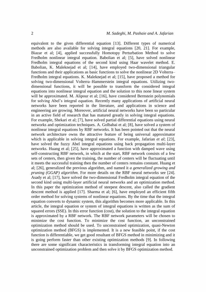
equivalent to the given differential equation [13]. Different types of numerical

methods are also available for solving integral equations [20, 21]. For example,

Biazar et al; [4], applied successfully Homotopy Perturbation Method to solve

Fredholm nonlinear integral equation. Babolian et al; [5], have solved nonlinear

Fredholm integral equations of the second kind using Haar wavelet method. E.

Babolian, K. Maleknejad et al; [14], have employed two-dimensional triangular

functions and their applications as basic functions to solve the nonlinear 2D Volterra–

Fredholm integral equations. K. Maleknejad et al; [15], have proposed a method for

solving two-dimensional Volterra–Hammerstein integral equations. Utilizing two-

dimensional functions, it will be possible to transform the considered integral

equations into nonlinear integral equation and the solution to this none linear system

will be approximated. M. Alipour et al; [16], have considered Bernstein polynomials

for solving Abel’s integral equation. Recently many applications of artificial neural

networks have been reported in the literature, and applications in science and

engineering are growing. Moreover, artificial neural networks have been so particular

in an active field of research that has matured greatly in solving integral equations.

For example, Shekari et al; [7], have solved partial differential equations using neural

networks and optimization techniques. A. Golbabai et al; [8], have solved a system of

nonlinear integral equations by RBF networks. It has been pointed out that the neural

network architecture owns the attractive feature of being universal approximator

which is applicable in solving integral equations. For example, Jafarian et al; [23],

have solved the fuzzy Abel integral equations using back propagation multi-layer

networks. Huang et al; [25], have approximated a function with damped wave using

self-constructing RBF network, in which at the start, RBF network consists of a few

sets of centers, then given the training, the number of centers will be fluctuating until

it meets the successful training then the number of centers remains constant. Huang et

al; [26], generalized the previous algorithm, and named it a generalized growing and

pruning (GGAP) algorithm. For more details on the RBF neural networks see [24].

Asady et al; [17], have solved the two-dimensional Fredholm integral equation of the

second kind using multi-layer artificial neural networks and an optimization method.

In this paper the optimization method of steepest descent, also called the gradient

descent method is applied [17]. Sharma et al; [6], have employed an efficient fifth

order method for solving systems of nonlinear equations. By the time that the integral

equation converts to dynamic system, this algorithm becomes more applicable. In this

article, the integral equation or system of integral equations is written as the sum of

squared errors (SSE). In this error function (cost), the solution to the integral equation

is approximated by a RBF network. The RBF network parameters will be chosen to

minimize the cost function. To minimize the cost function, an unconstrained

optimization method should be used. To unconstrained optimization, quasi-Newton

optimization method (BFGS) is implemented. It is a new feasible point, if the cost

function is differentiable, we get good resultant of BFGS method in minimizing and it

is going perform faster than other existing optimization methods [9]. In following

there are some significant characteristics in transforming integral equation into an

unconstrained optimization problem and then solve it by BFGS optimization method.

RBF Neural Networks Based on BFGS Optimization Method for Solving Integral Equations 3

I. RBF neural network has been implemented as a universal approximator for

different types, especially Fredholm equations of the second kind.

II. Application of this method is ordinary.

III. Comparing to other iterative methods, its convergence rate is high as in most

cases it devotes less than 5 minutes to perform the process. While having

gradient descent, it may reach up to 30 minutes. This method reduces

processing and increases speed.

2. BFGS OPTIMIZATION METHOD

To actually solve many technical processes, optimization methods are needed. Hence

optimization methods explore assumptions to varying parameters and suggest the best

way to change them. Optimization methods generally categorized to: constrained and

unconstrained. Since transforming constrained method into unconstrained method is

feasible, unconstrained optimization techniques are vitally important [10]. Here we

discuss methods for unconstrained optimization, including Nelder Mead method,

Newton method and quasi-Newton methods [18]. Obviously, BFGS method is one of

the most effective methods for unconstrained optimization [10, 9].this is one of the

quasi-Newton methods which uses approximations instead of Hessian inverse matrix

methods If we have the following minimization problem of the form

f( ), nMin x X R (1)

Given, *( )f x is the minimal, the iterative process for finding *x is:

1 ,T

k k k k kX X S f x (2)

Where kS is a symmetric matrix n n , and k is learning rate which will be found to

minimize 1( )kf x . For kS is Hessian matrix of, Newton's method will be found, and if

kS I then we have gradient descent. In general, choosing kS as one of the

approximation of Hessian matrix, quasi-Newton methods can be established.

Suppose f on nR contains the continuous second order partial derivatives, define

1,T

k k k k kg f x p X X (3)

And kH is Hessian matrix approximation in iteration k. Hence approximation of the

matrix H is applied by David-Fletcher-Powell.

Starting from each of the positive constant symmetric matrix 0H (i.e I), each point

0x and 0k take the following phases:


Phase 1. Consider

k k kd H g

Phase 2 .Minimize ( )k kf x d subject to 0 .

Now we have 1kX , k k kP d and 1kg obtained.

Phase 3. Consider

1k k kq g g

And

1

T T

k k k k k kk k T T

k k k k k

p p H q q HH H

p q q H q (4)

Then, Update k and return to step 1.

It is proven that if kH is real-valued constant, then 1kH will be real-valued constant

and the sequence of this algorithm is convergence [10]. A new method of updating for

H is, Broyden- Fletcher- Goldfarb-Shanno [10]:

1 1

T T T T

k k k k k k k k k k kk k T T T

k k k k k k

q H q p p p q H H q pH H

q p p q q p

(5)

Provided that in the above algorithm, state (5) is used instead of (4), the method will

be plausible as BFGS method.

Remark. It is proven that for each 0k which led to 0T

k kp q , also matrix 1kH

remains constant positive [Lu]. So at phase 2, we will start with small value of k and

then deploy it to the point that we get 0T

k kp q .

Respect to this, an optimization problem no longer need to be solved in the second

phase.

Example a. BFGS algorithm will be employed in solving the following minimizing

problem

2 45 25 8 f ,Min x xy y x y Min x y (6)

After the gradient vector is computed, starting from the initial point 0 20, 5X ,

BFGS algorithm will get running until the obtained absolute error from the four

previous errors (approximations) is small enough in other words:


9

413

1.2663 10

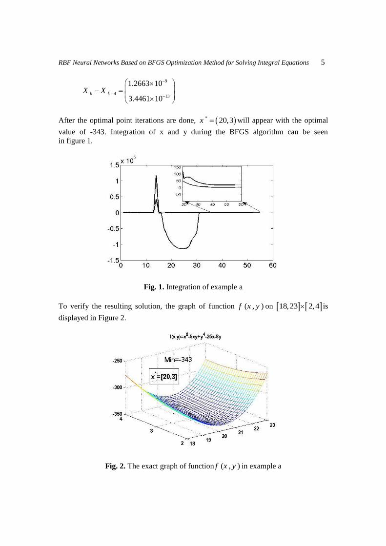
3.4461 10k kX X

After the optimal point iterations are done, * 20,3x will appear with the optimal

value of -343. Integration of x and y during the BFGS algorithm can be seen

in figure 1.

Fig. 1. Integration of example a

To verify the resulting solution, the graph of function ( , )f x y on 18,23 2,4 is

displayed in Figure 2.

Fig. 2. The exact graph of function ( , )f x y in example a


We see that running time is limited. In fact, when f is differentiable, this method is

superior to other methods.

3. ARTIFICIAL NEURAL NETWORK RBF

Artificial neural networks ANN have many uses in a variety of architecture to detect

function approximation. ANNs have given considerable attention in multi-layer

networks, radial basis function (RBF) networks and recursive networks. Radial basis

function (RBF) networks typically have three layers: an input layer, a hidden layer

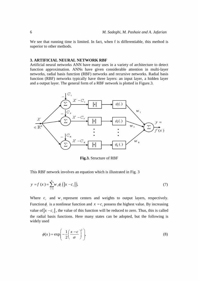
and a output layer. The general form of a RBF network is plotted in Figure.3.

Fig.3. Structure of RBF

This RBF network involves an equation which is illustrated in Fig. 3

1

( ) ,n

i i i

i

y f x w x c

(7)

Where ic and iw represent centers and weights to output layers, respectively.

Function i is a nonlinear function and ix c possess the highest value. By increasing

value of ix c , the value of this function will be reduced to zero. Thus, this is called

the radial basis functions. Here many states can be adopted, but the following is

widely used

21

( ) exp ,2

x cx

(8)


This function is called Gaussian function and σ is the variance.

And

2 2 2( ) ,i ix x c

(9)

Subject to 0

And α is not an even number. Function in (9), is called multiquadric. Width i can

be defined as mean absolute distance of origin point. And

1

, 2, ,1

k

k i

i

c k mk

(10)

Where ic i-th center and β is a real constant which is closed to one. The interesting

feature of multilayer neural networks and RBF network is that they are known as

universal approximator. The following theorem justifies that the RBF networks are

universal approximator

Theorem 1: Assume Ω is the set of all functions which are calculated by a Gaussian

network on a compact set of S includes nR .

2

1 1

1( ) exp : , , ,

2

N nk ik

N i i ik ik

i k ik

x cf x w w c X S

And

1

N

N

Now, Ω is dense in C S .

Proof. Refer to [11]

Having this theorem, it is proved that and by altering the function (0) , Each of

Gaussian RBF networks are universal approximator. (RBF) network has also been

used successfully in a variety of applications, and which has a number of advantages.

Selecting the numbers, spotting the centers and initial widths and how to update RBF

network become very crucial to understand these networks. If learning is supervised

in Gaussian networks, all optimized parameters will be achieved by using back

propagation (BP) method. By considering the function in (9), then intervals i are

provided from the equation (10), consequently, centers will be determined using

testing error as well as employing K – means clustering algorithm (K-M).

The algorithm then randomly chooses k points in vector space, these point serve as

the initial centers while the same distance measure is chosen [19].


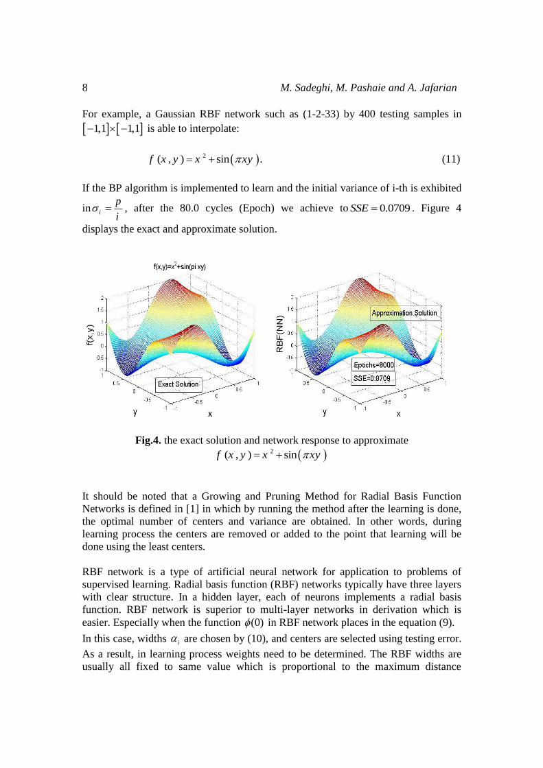
For example, a Gaussian RBF network such as (1-2-33) by 400 testing samples in

1,1 1,1 is able to interpolate:

2( , ) sin .f x y x xy (11)

If the BP algorithm is implemented to learn and the initial variance of i-th is exhibited

in i

p

i , after the 80.0 cycles (Epoch) we achieve to 0.0709SSE . Figure 4

displays the exact and approximate solution.

Fig.4. the exact solution and network response to approximate

2( , ) sinf x y x xy

It should be noted that a Growing and Pruning Method for Radial Basis Function

Networks is defined in [1] in which by running the method after the learning is done,

the optimal number of centers and variance are obtained. In other words, during

learning process the centers are removed or added to the point that learning will be

done using the least centers.

RBF network is a type of artificial neural network for application to problems of

supervised learning. Radial basis function (RBF) networks typically have three layers

with clear structure. In a hidden layer, each of neurons implements a radial basis

function. RBF network is superior to multi-layer networks in derivation which is

easier. Especially when the function (0) in RBF network places in the equation (9).

In this case, widths i are chosen by (10), and centers are selected using testing error.

As a result, in learning process weights need to be determined. The RBF widths are

usually all fixed to same value which is proportional to the maximum distance


between the chosen centers. Their excellent approximation capabilities have been one

of the advantages.

4. INTEGRAL EQUATIONS AND ITS RELATIONSHIP WITH NEURAL

NETWORKS

In this section, converting integral equations and integral equations systems to an

optimization problem has explained. Since in this method being linear and nonlinear

integral equation seems to be not an issue, it is stated as

( ) ( ) ( , ) ( ) , , ,f t F u t k t s G u s ds a b or a x

(12)

In general the equation (*), is diagnosed as a Volterra or Fredholm linear or nonlinear

integral equation, and it is assumed that equation (*) is second kind. In the other

words:

( ) 0F u t

We define:

( ) ( ) ( , ) ( ) .u t F u t k t s G u s ds

Therefore, equation (*) is written as follows:

1( ) ( ) 0,f t u t t

In which 1 is a set which is meant to find the solution to ( )u t , subject to 1t .

Consider the following cost function:

21

( , ) ( ) ( ) ;2 t B

E f f t u t

(13)

Where B is a subset of 1 , defined as the training data set. It is quite clear that for

such a function ˆ( )u t , the value of E on 1 is reached to the least possible value, then

ˆ( )u t is identified as a solution to the equation (*). Here, unknown function ˆ( )u t is

approximated by a RBF network. As a result, ˆ( )u t is considered RBF network, output

layer weights are unknown and E in (12) based on the weight of the output layer is a

function of multi-variables. We have explicitly included that weights are unknown.

Ultimately, the purpose is to find RBF weights so that the value of E in (13) is about

to minimized. To minimize E, the unconstrained Broyden Fletcher Goldfarb Shanno

(BFGS) optimization method will be used.


Remark 1. In finding cost function E, it is necessary to approximate certain integrals

by a numerical method. Of all proposed algorithm in this paper, Simpson and

Romberg numerical methods are less accurate and derivation of E is recognized

problematic.

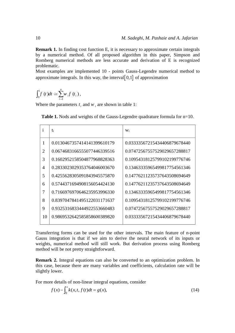
Most examples are implemented 10 - points Gauss-Legendre numerical method to

approximate integrals. In this way, the interval 0,1 of approximation

1

01

( ) ( )n

i i

i

f t dt w f t

,

Where the parameters it and iw are shown in table 1:

Table 1. Nods and weights of the Gauss-Legendre quadrature formula for n=10.

i ti wi

1

2

3

4

5

6

7

8

9

10

0.0130467357414141399610179

0.0674683166555077446339516

0.1602952158504877968828363

0.2833023029353764046003670

0.4255628305091843945575870

0.5744371694908156054424130

0.7166976970646235953996330

0.8397047841495122031171637

0.9325316833444922553660483

0.9869532642585858600389820

0.03333567215434406879678440

0.07472567557529029657288817

0.10954318125799102199776746

0.13463335965499817754561346

0.14776211235737643508694649

0.14776211235737643508694649

0.13463335965499817754561346

0.10954318125799102199776746

0.07472567557529029657288817

0.03333567215434406879678440

Transferring forms can be used for the other intervals. The main feature of n-point

Gauss integration is that if we aim to derive the neural network of its inputs or

weights, numerical method will still work. But derivation process using Romberg

method will be not pretty straightforward.

Remark 2. Integral equations can also be converted to an optimization problem. In

this case, because there are many variables and coefficients, calculation rate will be

slightly lower.

For more details of non-linear integral equations, consider

( ) ( , , ( ) ( ),x

f x k x t f t dt g x 0 (14)


Where

( ) ( ), ( ), , ( ) ,

( ) ( ), ( ), , ( ) ,

, , , ,, , ( ) , , ( ) , , ( ) , , ( )

T

n

T

n

T

n

f x f x f x f x

g x g x g x g x

k k k kx t f t x t f t x t f t x t f t

1 2

1 2

1 2

To solve the equation (1), unknown function f, is approximated by a RBF network

which is called ( , )NNrbf c r , in other words

( ) , ,f x NNrbf x c r (15)

In which c and r represent centers and Gaussian functions distances, respectively. X is

RBF input and ( )f x is RBF output. After approximation of (2), and replace it in (1), it

must be provided a function of energy (costs) to be minimized. Note that ( )f x is a

vector.

Creating energy function, the interval ,a b is recommended to solve equation (1).

Then some points such as ix from ,a b is selected which are called data training set.

For each ix , the error is calculated as follows:

, , , , , , ( )ix

i i i i iNNrbf x c r k x t NNrbf x c r dt g x 0 (16)

Note that equation (3) is a vector. To complete the energy function, for different i ,

least squares of vector i is considered. Thus, the energy function is stated as follows:

2

1

,d

ii

E NN

(17)

Where d is the number of training data, 2

i is square of component i and 0 goes as

1

.k

i

i

xx

(18)

Subject to 1, ,t

kx x x

Finally, the unconstrained optimization problem is provided.

,

,c r

E Min E NN

Where ( )E NN is multi-variable function with the unknown’s c and r which need to be

defined that the resulting value will be the lowest. The process of obtaining c and r is

the learning network. In computer program, you should note that the index

components of the unknown vector function ( )f x are not pressed wrong because it

lead us to a wrong solution.


5. NUMERICAL RESULTS AND EXAMPLES

In this section, some examples on effectiveness of proposed algorithm for solving

integral equations are investigated. In each example, properties and optimal

parameters before and after the learning network will be mentioned. This method is

used for a variety of integral equations but Fredholm equations of the first kind.

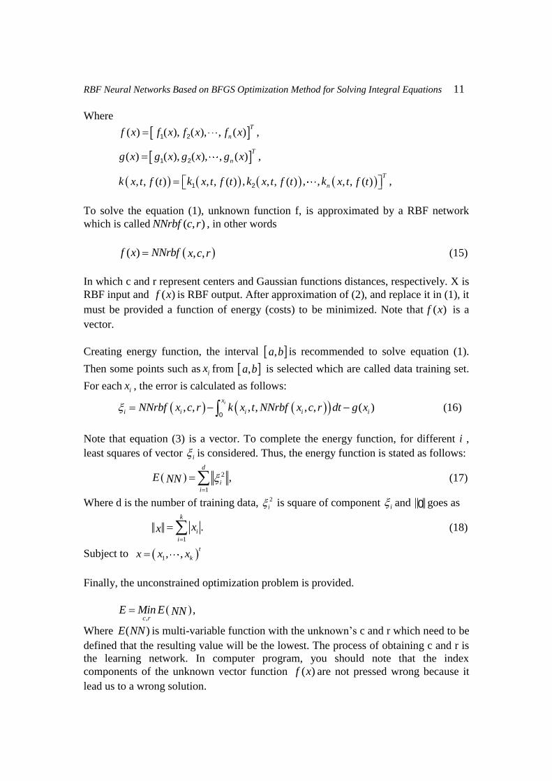
Example 1. Fredholm integral equation of the second kind is given:

2

0

1( ) sin( ) sin( )cos( ) ( )

2u x x x t u t dt

The exact solution is ( ) sinu x x . After the desired learning network is created,

properties of network will be detected. RBF network centers are

0.05,0.1,0.2,0.3,0.4,0.5,0.55,0.6,0.7,0.75,0.8,0.85,0.9,1,1.1,1.15,1.2,1.3,1.4,1.45,1.5 ;c

The interval 0,2

divided into 10 equal parts and the obtained points are training

data. In each of iteration, Simpson numerical method with 8 points is employed to

approximate integrals. After learning network, the least square error is obtained.

288.937129 10E

The level of error in the specified points of interval 0,2

can be seen in table 2.

After converting (15) to an unconstrained optimization problem and solving the

problem by using Nelder-Mead, results to ( )u x will be obtained (table 2).

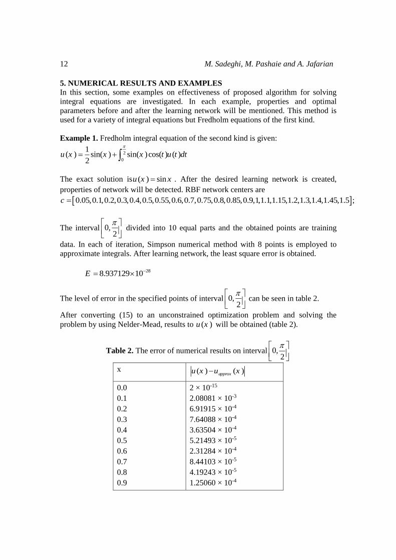
Table 2. The error of numerical results on interval 0,2

x ( ) ( )approxu x u x

0.0

0.1

0.2

0.3

0.4

0.5

0.6

0.7

0.8

0.9

2 × 10-15

2.08081 × 10-3

6.91915 × 10-4

7.64088 × 10-4

3.63504 × 10-4

5.21493 × 10-5

2.31284 × 10-4

8.44103 × 10-5

4.19243 × 10-5

1.25060 × 10-4


1

1.1

1.2

1.3

1.4

1.5

1.37210 × 10-4

9.90674 × 10-5

1.15926 × 10-4

1.65118 × 10-4

1.30257 × 10-4

3.26301 × 10-5

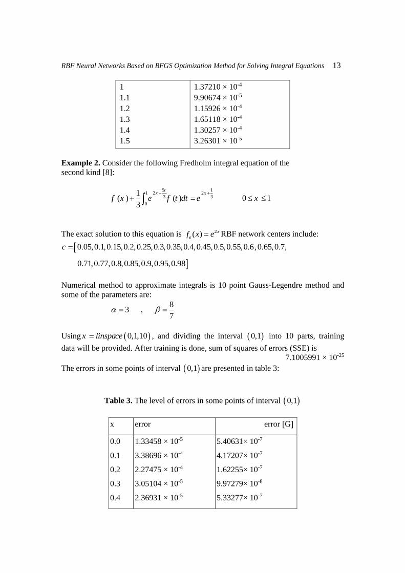
Example 2. Consider the following Fredholm integral equation of the

second kind [8]:

5 12 21

3 3

0

1( ) ( ) 0 1

3

tx x

f x e f t dt e x

The exact solution to this equation is 2( ) x

ef x e RBF network centers include:

0.05,0.1,0.15,0.2,0.25,0.3,0.35,0.4,0.45,0.5,0.55,0.6,0.65,0.7,

0.71,0.77,0.8,0.85,0.9,0.95,0.98

c

Numerical method to approximate integrals is 10 point Gauss-Legendre method and

some of the parameters are:

8

3 ,7

Using 0,1,10x linspace , and dividing the interval 0,1 into 10 parts, training

data will be provided. After training is done, sum of squares of errors (SSE) is 25-10 7.1005991 ×

The errors in some points of interval 0,1 are presented in table 3:

Table 3. The level of errors in some points of interval 0,1

x error [G]error

0.0

0.1

0.2

0.3

0.4

1.33458 × 10-5

3.38696 × 10-4

2.27475 × 10-4

3.05104 × 10-5

2.36931 × 10-5

5.40631× 10-7

4.17207× 10-7

1.62255× 10-7

9.97279× 10-8

5.33277× 10-7


0.5

0.6

0.7

0.8

0.9

1

6.02424 × 10-5

1.54610 × 10-5

8.62065 × 10-5

2.77102 × 10-5

1.29511 × 10-4

9.86130 × 10-5

5.12821× 10-7

8.86581× 10-8

3.82386× 10-7

6.76977× 10-7

3.36868× 10-7

5.00635× 10-7

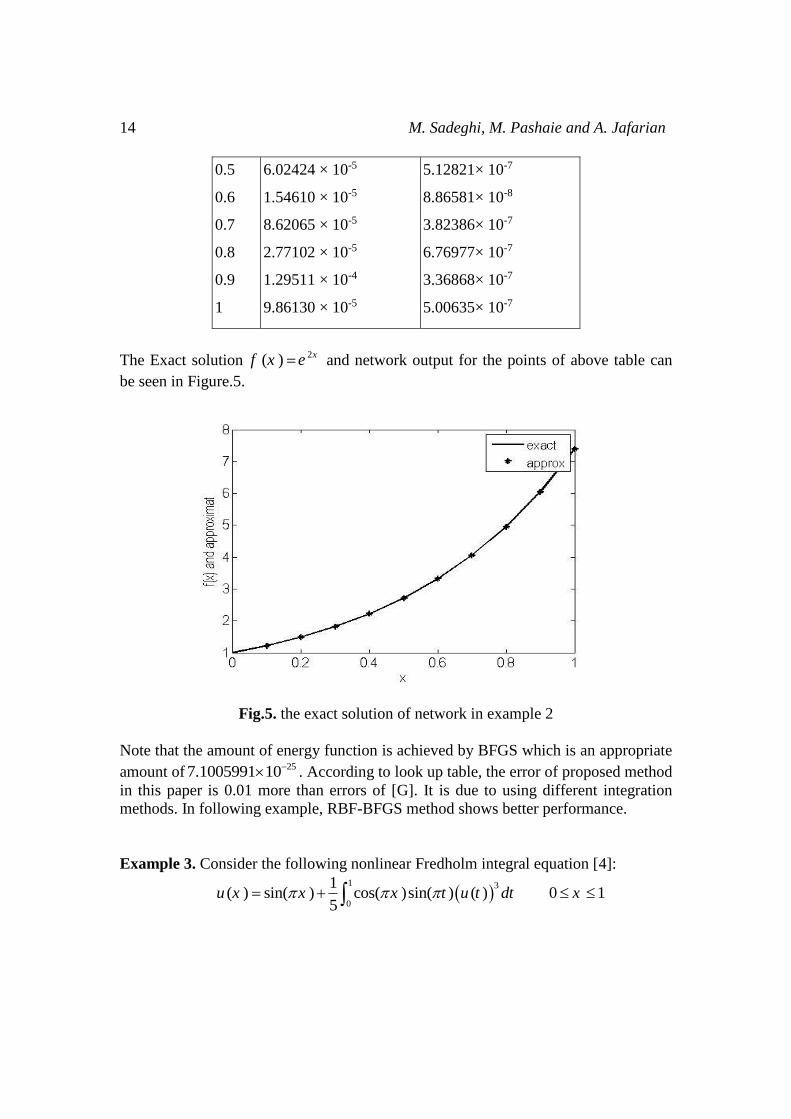
The Exact solution 2( ) xf x e and network output for the points of above table can

be seen in Figure.5.

Fig.5. the exact solution of network in example 2

Note that the amount of energy function is achieved by BFGS which is an appropriate

amount of257.1005991 10 . According to look up table, the error of proposed method

in this paper is 0.01 more than errors of [G]. It is due to using different integration

methods. In following example, RBF-BFGS method shows better performance.

Example 3. Consider the following nonlinear Fredholm integral equation [4]:

1 3

0

1( ) sin( ) cos( )sin( ) ( ) 0 1

5u x x x t u t dt x


The exact solution is20 391

( ) sin( ) cos( )3

u x x x

. Network centers are

selected as previous example. And most of the parameters are constant. 10-point

Gauss integration method is implemented.

After training is done, sum of squares of errors (SSE) is 9.92589 × 10-24.

The integral equation in [4] is solved by Homotopy Perturbation method. The errors

are shown in table 4.

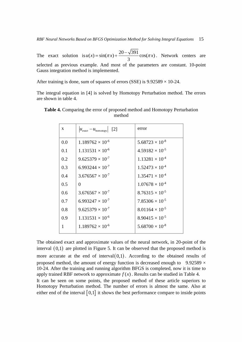
Table 4. Comparing the error of proposed method and Homotopy Perturbation

method

x homexact otopyu u [2] error

0.0

0.1

0.2

0.3

0.4

0.5

0.6

0.7

0.8

0.9

1

1.189762 × 10-6

1.131531 × 10-6

9.625379 × 10-7

6.993244 × 10-7

3.676567 × 10-7

0

3.676567 × 10-7

6.993247 × 10-7

9.625379 × 10-7

1.131531 × 10-6

1.189762 × 10-6

5.68723 × 10-8

4.59182 × 10-5

1.13281 × 10-4

1.52473 × 10-4

1.35471 × 10-4

1.07678 × 10-4

8.76315 × 10-5

7.85306 × 10-5

8.01164 × 10-5

8.90415 × 10-5

5.68700 × 10-8

The obtained exact and approximate values of the neural network, in 20-point of the

interval 0,1 are plotted in Figure 5. It can be observed that the proposed method is

more accurate at the end of interval 0,1 . According to the obtained results of

proposed method, the amount of energy function is decreased enough to 9.92589 ×

10-24. After the training and running algorithm BFGS is completed, now it is time to

apply trained RBF network to approximate ( )f x . Results can be studied in Table 4.

It can be seen on some points, the proposed method of these article superiors to

Homotopy Perturbation method. The number of errors is almost the same. Also at

either end of the interval 0,1 it shows the best performance compare to inside points


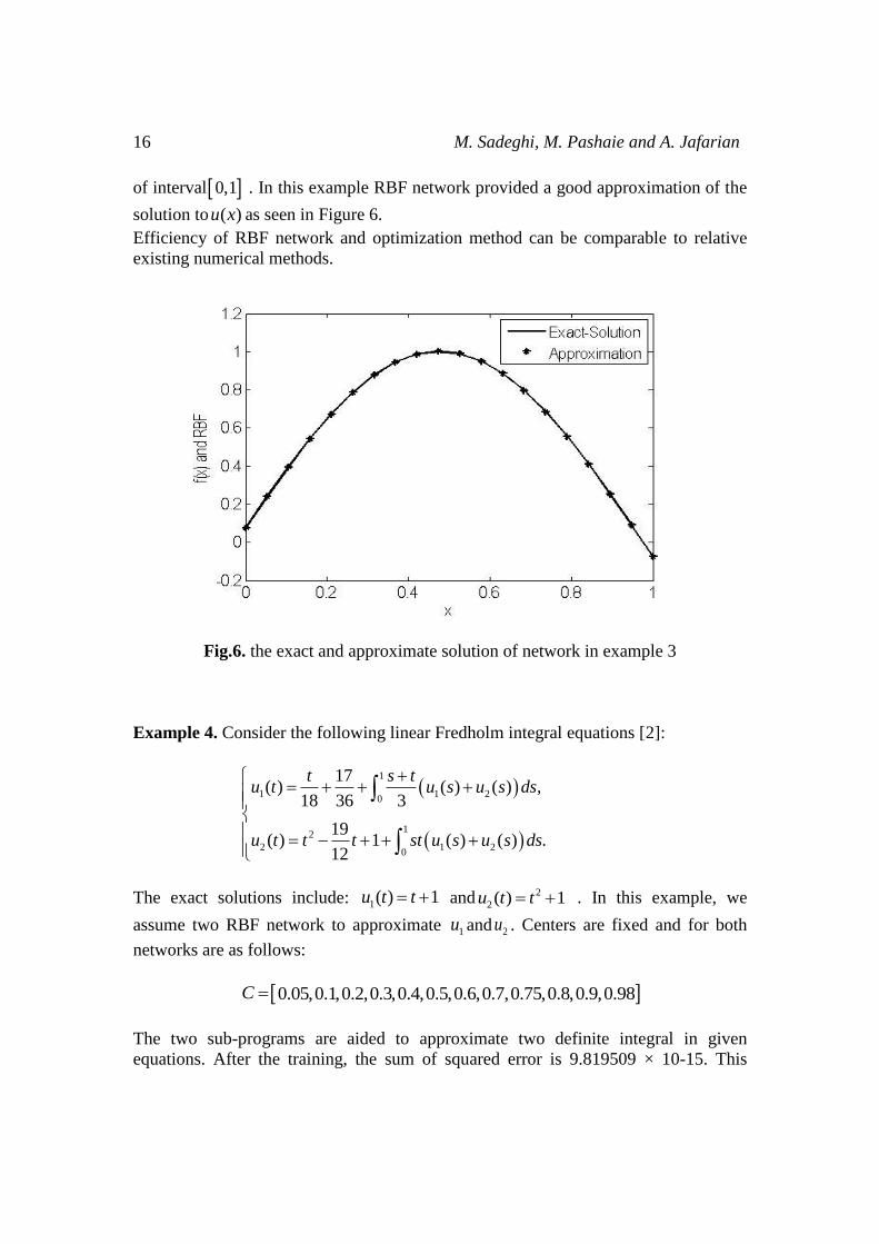
of interval 0,1 . In this example RBF network provided a good approximation of the

solution to ( )u x as seen in Figure 6.

Efficiency of RBF network and optimization method can be comparable to relative

existing numerical methods.

Fig.6. the exact and approximate solution of network in example 3

Example 4. Consider the following linear Fredholm integral equations [2]:

1

1 1 20

12

2 1 20

17( ) ,( ) ( )

18 36 3

19( ) 1 .( ) ( )

12

t s tu t dsu s u s

u t t t st dsu s u s

The exact solutions include: 1( ) 1u t t and 2

2( ) 1u t t . In this example, we

assume two RBF network to approximate 1u and 2u . Centers are fixed and for both

networks are as follows:

0.05,0.1,0.2,0.3,0.4,0.5,0.6,0.7,0.75,0.8,0.9,0.98C

The two sub-programs are aided to approximate two definite integral in given

equations. After the training, the sum of squared error is 9.819509 × 10-15. This


example in [t] has been solved using analyzing method. The values obtained from

proposed method in this article and analyzing method are displayed in table 5.

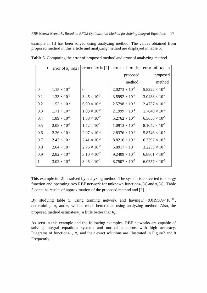
Table 5. Comparing the error of proposed method and error of analyzing method

t [2]in 1uerror of [2]in 2uerror of in 1uerror of

proposed

method

in 2uerror of

proposed

method

0

0.1

0.2

0.3

0.4

0.5

0.6

0.7

0.8

0.9

1

1.15 × 10-2

1.33 × 10-2

1.52 × 10-2

1.71 × 10-2

1.89 × 10-2

2.08 × 10-2

2.26 × 10-2

2.45 × 10-2

2.64 × 10-2

2.82 × 10-2

3.02 × 10-1

0

3.45 × 10-3

6.90 × 10-3

1.03 × 10-2

1.38 × 10-2

1.72 × 10-2

2.07 × 10-2

2.41 × 10-2

2.76 × 10-2

3.10 × 10-2

3.45 × 10-2

2.0273 × 10-5

3.5992 × 10-4

2.5798 × 10-4

2.1999 × 10-4

5.2762 × 10-5

1.0913 × 10-4

2.8376 × 10-5

8.8216 × 10-5

5.8917 × 10-5

9.2409 × 10-5

8.7507 × 10-5

5.8222 × 10-9

3.0438 × 10-4

2.4737 × 10-4

1.7840 × 10-4

6.5656 × 10-5

8.1042 × 10-5

5.8746 × 10-6

6.3392 × 10-5

3.2255 × 10-5

6.8801 × 10-5

6.0757 × 10-5

This example in [2] is solved by analyzing method. The system is converted to energy

function and operating two RBF network for unknown function 1( )u x and 2 ( )u x . Table

5 contains results of approximation of the proposed method and [2].

By studying table 5, using training network and having169.819509 10E ,

determining 1u and 2u will be much better than using analyzing method. Also, the

proposed method estimates 2u a little better than 1u .

As seen in this example and the following examples, RBF networks are capable of

solving integral equations systems and normal equations with high accuracy.

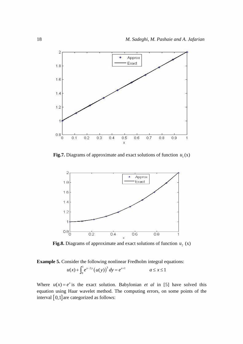
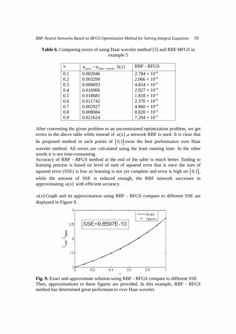
Diagrams of function 1u , 2u and their exact solutions are illustrated in Figure7 and 8

Frequently.


Fig.7. Diagrams of approximate and exact solutions of function 1u (x)

Fig.8. Diagrams of approximate and exact solutions of function 2u (x)

Example 5. Consider the following nonlinear Fredholm integral equations:

1 32 1

0( ) 1( )

x y xu x e dy e a xu y

Where ( ) xu x e is the exact solution. Babylonian et al in [5] have solved this

equation using Haar wavelet method. The computing errors, on some points of the

interval 0,1 are categorized as follows:


Table 6. Comparing errors of using Haar wavelet method [5] and RBF-BFGS in

example 5

RBF - BFGS exact Haar waveletu u [k1] x

2.784 × 10-4

2.066 × 10-4

4.654 × 10-5

2.927 × 10-4

1.818 × 10-3

2.370 × 10-4

4.860 × 10-4

8.820 × 10-3

7.294 × 10-3

0.002046

0.003299

0.008693

0.016906

0.018681

0.011742

0.002927

0.008084

0.021624

0.1

0.2

0.3

0.4

0.5

0.6

0.7

0.8

0.9

After converting the given problem to an unconstrained optimization problem, we get

errors in the above table while instead of ( )u x ,a network RBF is used. It is clear that

he proposed method in each points of 0,1 owns the best performance over Haar

wavelet method. All errors are calculated using the least running time. In the other

words it is not time-consuming.

Accuracy of RBF - BFGS method at the end of the table is much better. Ending to

learning process is based on level of sum of squared error that is once the sum of

squared error (SSE) is low so learning is not yet complete and error is high on 0,1 ,

while the amount of SSE is reduced enough, the RBF network successes in

approximating ( )u x with efficient accuracy.

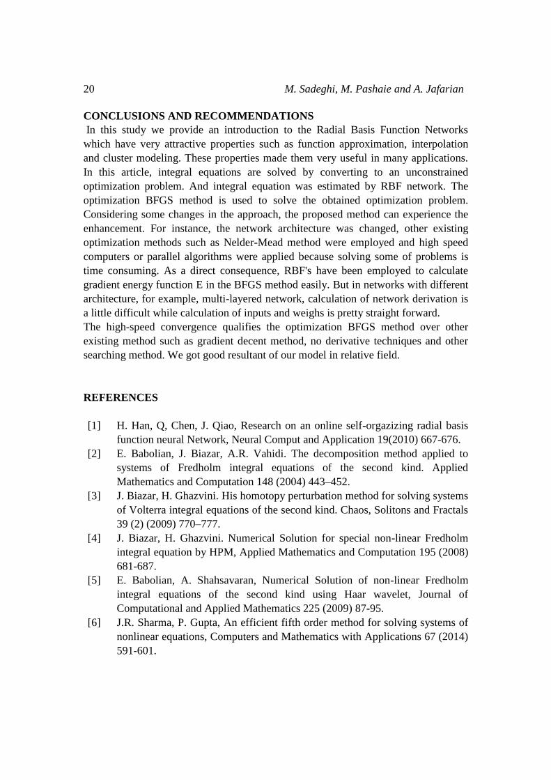
( )u x Graph and its approximation using RBF - BFGS compare to different SSE are

displayed in Figure 9.

Fig. 9. Exact and approximate solution using RBF - BFGS compare to different SSE

Then, approximations to these figures are provided. In this example, RBF - BFGS

method has determined great performances over Haar wavelet.


CONCLUSIONS AND RECOMMENDATIONS

In this study we provide an introduction to the Radial Basis Function Networks

which have very attractive properties such as function approximation, interpolation

and cluster modeling. These properties made them very useful in many applications.

In this article, integral equations are solved by converting to an unconstrained

optimization problem. And integral equation was estimated by RBF network. The

optimization BFGS method is used to solve the obtained optimization problem.

Considering some changes in the approach, the proposed method can experience the

enhancement. For instance, the network architecture was changed, other existing

optimization methods such as Nelder-Mead method were employed and high speed

computers or parallel algorithms were applied because solving some of problems is

time consuming. As a direct consequence, RBF's have been employed to calculate

gradient energy function E in the BFGS method easily. But in networks with different

architecture, for example, multi-layered network, calculation of network derivation is

a little difficult while calculation of inputs and weighs is pretty straight forward.

The high-speed convergence qualifies the optimization BFGS method over other

existing method such as gradient decent method, no derivative techniques and other

searching method. We got good resultant of our model in relative field.

REFERENCES

[1] H. Han, Q, Chen, J. Qiao, Research on an online self-orgazizing radial basis

function neural Network, Neural Comput and Application 19(2010) 667-676.

[2] E. Babolian, J. Biazar, A.R. Vahidi. The decomposition method applied to

systems of Fredholm integral equations of the second kind. Applied

Mathematics and Computation 148 (2004) 443–452.

[3] J. Biazar, H. Ghazvini. His homotopy perturbation method for solving systems

of Volterra integral equations of the second kind. Chaos, Solitons and Fractals

39 (2) (2009) 770–777.

[4] J. Biazar, H. Ghazvini. Numerical Solution for special non-linear Fredholm

integral equation by HPM, Applied Mathematics and Computation 195 (2008)

681-687.

[5] E. Babolian, A. Shahsavaran, Numerical Solution of non-linear Fredholm

integral equations of the second kind using Haar wavelet, Journal of

Computational and Applied Mathematics 225 (2009) 87-95.

[6] J.R. Sharma, P. Gupta, An efficient fifth order method for solving systems of

nonlinear equations, Computers and Mathematics with Applications 67 (2014)

591-601.


[6] Shekari Bidokhti, A. Malik, Solving initial boundary value problems for

systems of partial differential equations using neural networks and

optimization techniques, Journal of the Franklin Institute 346 (2009) 898-913.

[8] A. Golbabai b, M. Mammadova, S. Seifollahi, Solving a system of nonlinear

integral equations by an RBF network, Computers and Mathematics with

Applications. 57 (2006). 1651-1658.

[9] M.S. Bazarea, C.M. Shetty, Nonlinear Programming, Theory and Algorithms,

John Wiley and Sons, NewYork, 1990.

[10] D.G. Luenberger, Introduction to linear and nonlinear Programming, Reading,

MA: addision-Wesley 1984.

[11] M.M. Gupta, L. Jin, and N. Homma, Static and dynamic neural networks, John

Wiley and Sons, Inc, Simultaneously in Canada, (2003).

[12] K. Atkinson, W. Han, Theoretical Numerical Analysis: a Functional Analysis

Framework, Springer-Verlag, NewYork, INC, (2001)

[13] A. Jerri, Introduction to Integral Equations with Applications, INC, John

Wiley and Sons, (1999).

[14] E. Babolian, K. Maleknejad, M. Roodaki, H. Almasieh, Two-dimensional

triangular functions and their applications to nonlinear 2D Volterra–Fredholm

integral equations, Comput, Math. Appl. 60, 1711-1722, (2010).

[15] M. Maleknejad, S. Sohrabi, B. Baranji, Two dimensional PCBF s application

to nonlinear Volterra integral equations, in: Proceedings of the world, (2009).

[16] M. Alipour, D. Rostamy, Bernstein polynomials for solving Abel’s integral

equation, The Journal of Mathematics and Compuret Science Vol. 3, No. 4,

403-412, (2011).

[17] B. Asady, F. Hakimzadegan, R. Nazarlu, Utilizing. Artifical neural network

approach for solving two-dimensional integral equations, Math, Sci, (2014), 8-

117.

[18] S.S. Rao, Engineering Optimization, Theory and Practice, Purdue University,

West Lafayette, Hndiana, (1996).

[19] Laurene V. Fausett, Fundamentals of Neural Networks, practice Hall, (2001).

[20] Atkinson, K.E., The Numerical Solution of Integral equations of the Second

kind, Cambridge, Cambridge, University Press (1997).

[21] Wazwaz, A.M., A First course in integral equations, World Scientific,

Signapore (1997).

[22] Bidokhti, Sh, Malek, A., Solving initial boundary Nalue problems for systems

of partial differential equations using neural networks and optimization

techniques, Sournal of the Franklin Institute 34, (2009), 898-913.

[23] Jafarian, A., Measoomy Nia, S., Artificial neural network approach to the

fuzzy Abel integral equation problem. Journal of Intelligent fuzzy sys.

27(2014), 83-91.

[24] Gupta, M.M., Jin, L., Homma, N., Static and dynamic neural networks, A

John Wiley and Sons, INC., Publication., Hoboken, New. Jersey (2003).

[25] Huang, G.B., Saratchandran, P., Sundararajan, N., An efficient sequential

learning algorithm for growing and pruning RBF (GAP-RBF) network IEEE

Trans Syst Man Cyben B 34 (6)(2004) 2284-2292.

http://www.sciencedirect.com/science/article/pii/S0898122110004773








[26] Huang, G.B., Saratchandran, P. Sundararajan, N., A generalized growing and

pruning RBF (GGAP-RBF) neural networks for function approximation, IEEE

Trans neural net. 16(1) (2005), 57-67.

Documents

RBF Neural Networks Based on BFGS Optimization Method for ... · Numerical Solution of integral equations plays major role in applications of sciences ... Fredholm integral equations