Embed Size (px)
Citation preview
This document is downloaded from DR‑NTU (https://dr.ntu.edu.sg)Nanyang Technological University, Singapore.
Condition based management of gas turbineengine using neural networks
Muthukumar, Krishnan
2005
Muthukumar, K. (2005). Condition based management of gas turbine engine using neuralnetworks. Master’s thesis, Nanyang Technological University, Singapore.
https://hdl.handle.net/10356/6556
https://doi.org/10.32657/10356/6556
Nanyang Technological University
Downloaded on 13 Feb 2022 11:27:18 SGT
CONDITION BASED MANAGEMENT OF
GAS TURBINE ENGINE USING NEURAL
NETWORKS
KRISHNAN MUTHUKUMAR
SCHOOL OF MECHANICAL & AEROSPACE ENGINEERING
NANYANG TECHNOLOGICAL UNIVERSITY
2005
ATTENTION: The Singapore Copyright Act applies to the use of this document. Nanyang Technological University Library
Condition Based Management of Gas
Turbine Engine Using Neural Networks
KRISHNAN MUTHUKUMAR
School of Mechanical & Aerospace Engineering
A thesis submitted to the Nanyang Technological University
in fulfilment of the requirement for the degree of
Master of Engineering
2005
ATTENTION: The Singapore Copyright Act applies to the use of this document. Nanyang Technological University Library
ABSTRACT _____________________________________________________________________________________________
Accurate prognostic models capable of predicting the performance degradation of the
industrial gas turbine are critical for improving plant profitability, by reducing the cost of energy
production and contributing to a cleaner environment. The main focus of this research work is to
develop an accurate steady state prognostic model to predict the performance degradation of gas
turbine compressor using Artificial Intelligence. The data for this research work have been taken
from the gas turbine operating in a combined cycle power plant using natural gas.
As a part of this research, the following works have been done. Thermodynamic models
are developed to find out gas turbine health indicating parameters like polytropic and isentropic
efficiencies of compressor, gross thermal efficiency, heat rate, compressor pressure ratio and air
flow rate. Various gas turbine operating parameters, design parameters and different
thermodynamic tables are used in these models to determine the gas turbine health indicating
parameters, since they are not measured directly.
Gas turbine performance depends not only on component degradation, but also on the
ambient condition, load level, fuel type and specific installation hardware such as inlet and outlet
ducting. In order to identify the real component’s degradation, methodology to correct the data
to the reference ambient condition has been incorporated into the developed models. The ISO
standard recommends the user to use the correction factors given by the gas turbine supplier for
the gas turbines used for the constant speed application, whereas it provides standard correction
formula for the gas turbines used for variable speed application. This recommendation is mainly
to avoid the dispute between the seller and buyer in meeting the guaranteed power output and
heat rate. The thermodynamic models are developed based on both the supplier and the standard
correction methodologies in order to find out their effects on the long term trending of the gas
turbine health indicating parameters and also to make the developed model more generic, i.e.
applicable to variable speed gas turbines also.
These corrected gas turbine health indicating parameters are then compared with the non
degraded values. Non degraded gas turbine data are based on gas turbine performance
acceptance tests performed immediately after commissioning, i.e. when the condition of the gas
turbine is clean and good. But the performance acceptance tests have been conducted for 60%,
85%, 93% and 100% loads only. In order to determine the gas turbine health indicating
parameters for the intermediate loads ranging from 60% to 100%, the curve fitting technique has
been used to find out the best suitable curve and its equation for the performance tests readings. Condition based management of gas turbine engine using neural networks
i
ATTENTION: The Singapore Copyright Act applies to the use of this document. Nanyang Technological University Library
ABSTRACT _____________________________________________________________________________________________
The on-line, off-line washing and inlet guide vane cleaning activities would reduce the
gas turbine’s compressor degradation rates. The hybrid neural network model is developed using
the Matlab tool-box to analyze the gas turbine compressor degradation. Various pre and post
processing techniques and network layers have been used in the developed hybrid neural
network model, and the best suitable technique has been selected. This hybrid neural network
model is trained with gas turbine health indicating parameters trended for about 15000
Equivalent operating hours. The developed hybrid neural model learn the effects of on-line, off-
line washing and inlet guide vane cleaning activities on the gas turbine’s compressor degradation
and predicts the gas turbine’s compressor degradation rates. The verification of this model with
the actual values has been done in order to find out their match with the real system. These
predictions are compared with the expected and guaranteed values given by the gas turbine
supplier. Maintenance decisions are suggested based on the deviation of the predicted gas
turbine’s compressor degradation with the expected values. The effect of cost has also been
included in analyzing the performance of the gas turbine driving the generator.
The degradation rates vary greatly and are specific to each plant depending on the site
location, surrounding environment, climatic conditions and plant layout. The adaptive nature of
the neural network model allows the user to tune to the model specific to the particular gas
turbine.
The study of different variants of the steady state model revealed that the hybrid neural
network developed has the ability to replicate the complicated gas turbine’s compressor
degradation with great accuracy. It mainly depends on the extent and variety of training data
available, type of pre-processing carried out, the choice of training method and the transfer
function used. The evolution of the model shows it is a good tool to measure the condition of the
gas turbine’s compressor health for both constant speed and variable speed application.
The cost analysis of the model explains that even 1 MWhr of energy loss per hour due to
the improper washing schedule leads to approximately half million dollar loss per annum.
Normally the off-line washing plus compressor Inlet guide vane blade cleaning are done during
the minor outages. (i.e. every 4000 equivalent operating hours). If one additional off-line
washing plus compressor blade cleaning is performed in between this period, it results in good
amount of energy saving of about 3960MWhr per 4000 equivalent operating hours. This energy
saving is overridden by the power generation opportunity lost cost. It could be minimized by Condition based management of gas turbine engine using neural networks
ii
ATTENTION: The Singapore Copyright Act applies to the use of this document. Nanyang Technological University Library

ABSTRACT _____________________________________________________________________________________________
Condition based management of gas turbine engine using neural networks
iii
conducting the following changes. The power selling prices are very low during week ends and
public holidays, if 2.5 days required for the manual washing is covered during in one of these
days will leads to good amount of energy and cost savings. The gas turbine availability is around
92% per annum and planned outages are about 3%. The balance 5% is due to breakdown
maintenance. The proper usage of this breakdown maintenance period (5%) could save around
8000MWhr of energy per annum.
The current research work is focused on the development of the hybrid neural network
model to asses the gas turbine’s compressor health and to suggest the appropriate washing
schedule including the cost effects also. It is recommended that this could be extended to assess
the degradation of the entire combined cycle power plant including other components such as
turbine , combustor and heat recovery steam generator.
ATTENTION: The Singapore Copyright Act applies to the use of this document. Nanyang Technological University Library

ACKNOWLEDGEMENT ________________________________________________________________________
The author would like to extend his gratitude to the following persons whose help
have gone a long way in the progress of this project.
A special thanks goes to Prof. Ho Hiang Kwee, whose knowledge in the field of
gas turbine and their diagnostics systems have been an inspiration to me. He has gone to
great extent with his invaluable guidance, advice and encouragement to me. The author is
also sincerely grateful for his patience and understanding throughout the course of the
research work.
Thanks also goes to the SIEMENS Pte Ltd manager’s Mr. Stefan Schaab and
Mr. Nareshkumar Wadwani for providing the valuable informations and practical views
about the industrial gas turbines, which is instrumental in linking of ideas and
information for this research work. Last but not least the author wishes to thank all his
friends for their great support for the successful completion this research work.
________________________________________________________________________ Condition based management of gas turbine engine using neural networks
iv
ATTENTION: The Singapore Copyright Act applies to the use of this document. Nanyang Technological University Library
TABLE OF CONTENTS ______________________________________________________________________________
Abstract Acknowledgement Table of Contents List of Figures List of Tables List of Symbols used
i iv v viii xiii xv
1 Introduction 1.1 Background 1 1.2 Objective 2 1.3 Approach 3
2 Literature Review 2.1 Combined cycle concept 6 2.2 Classification of gas turbine degradation 9 2.3 Compressor fouling and cleaning 9 2.4 Effects of various ambient factors on the combined cycle
performance 15
2.5 Correction of test results to reference conditions 20 2.6 Introduction to the gas turbine controllers for CCPP 29 2.7 Neural networks and artificial intelligence 32 2.8 Introduction to develop the neural network model using
Matlab toolbox 50
3 Model Development 3.1 Gas turbine degradation models development 55 3.2 Development of thermodynamic models to assess the gas
turbine compressor performance 55
3.3 Compressor washing details 64 3.4 Development of hybrid neural network models to assess the gas
turbine compressor performance 65
4 Results & Discussions 4.1 Overview of thermodynamic model results 77 4.2 Gas turbine compressor performance assessment using hybrid
neural network models 112
5 Conclusion and Recommendations 5.1 Conclusion 143 5.2 Recommendations on scheduling of compressor washing 143 5.3 Challenges and Recommendations for future work 145 References 147
______________________________________________________________________________ Condition based management of gas turbine engine using neural networks
v
ATTENTION: The Singapore Copyright Act applies to the use of this document. Nanyang Technological University Library
TABLE OF CONTENTS ______________________________________________________________________________
Appendix A Standard correction curves based on ISO 2314 (1998) for CCPP Appendix A1
Calculation of polytropic, isentropic efficiencies and pressure ratio of
gas turbine compressor
Appendix A2
Calculation of generator gross power output, efficiency & losses Appendix A3
Calculation of calorific value and carbon hydrogen ratio of fuel gas Appendix A4
Correction of Power output to reference conditions based on OEM
corrections
Appendix A5
Correction of Heat rate to reference conditions based on OEM
corrections
Appendix A6
Correction of Power output to reference conditions based on STD
corrections
Appendix A7
Procedure for calculating the corrected CCPP gross efficiency Appendix A8
Air flow rate calculation using combustion analysis Appendix A9
Mass and Energy balance method to find out the compressor inlet air
flow rate
Appendix A10
Gas turbine compressor washing details Appendix A11
Appendix B
Determination of compressor polytropic efficiency, isentropic
efficiency, generator efficiency and CCPP gross thermal efficiency
and its correction based on OEM
Appendix B1
Determination of compressor polytropic efficiency, isentropic
efficiency, generator efficiency and CCPP gross thermal efficiency
and its correction based on STD
Appendix B2
Matlab modeling - Air flow rate calculation using combustion analysis Appendix B3
Matlab modeling – Indirect air flow calculation using mass and energy
balance method
Appendix B4
Gas turbine compressor health monitoring using hybrid neural
network model based on Prestd preprocessing technique
Appendix B5
______________________________________________________________________________ Condition based management of gas turbine engine using neural networks
vi
ATTENTION: The Singapore Copyright Act applies to the use of this document. Nanyang Technological University Library
TABLE OF CONTENTS ______________________________________________________________________________
______________________________________________________________________________ Condition based management of gas turbine engine using neural networks
vii
Appendix C
Compressor polytropic, isentropic efficiency, pressure ratio and
CCPP gross thermal efficiency determination based on OEM
corrections
Appendix C1
Compressor polytropic, isentropic efficiency, pressure ratio and
CCPP gross thermal efficiency determination based on STD
corrections
Appendix C2
Gas turbine compressor inlet air flow rate using combustion analysis Appendix C3
Comparison of Indirect air flow calculation using Mass and Energy
balance method with OEM values
Appendix C4
Indirect air flow rate calculation using Mass and Energy balance
method for various EOH
Appendix C5
Appendix D
Thermal assessment of gas turbine engine using the hybrid neural
network models
Appendix D1
Cost Estimation of power generation cost and maintenance work cost Appendix D2
ATTENTION: The Singapore Copyright Act applies to the use of this document. Nanyang Technological University Library
LIST OF FIGURES
Figure 1.1 Classification of losses leading to overall gas turbine performance
degradation. 3
Figure 1.2 Thermodynamic model of compressor fouling 4
Figure 1.3 Summary of the Research work 5
Figure 2.1 Combined cycle power plant 6
Figure 2.2 Sankey diagram of a CCPP 7
Figure 2.3 Siemens V94.3A gas turbine engine general arrangement 8
Figure 2.4 Schematic Diagram of the single shaft CCPP 8
Figure 2.5 Typical effect of on-line and off-line compressor wet cleaning 13
Figure 2.6 Effect of Ambient Temperature 16
Figure 2.7 Effect of Ambient Pressure 16
Figure 2.8 Effect of Humidity on Power Output and exhaust flow 17
Figure 2.9 Effect of Compressor inlet pressure loss 18
Figure 2.10 Effect of Turbine Exhaust pressure loss 18
Figure 2.11 Effect of Speed on the Power Output and Exhaust flow 19
Figure 2.12 Correction curve of CCPP Output vs Ambient temperature Appendix A1-1
Figure 2.13 Correction curve of CCPP Output vs atmospheric pressure Appendix A1-1
Figure 2.14 Correction curve of CCPP Output vs
Ambient relative humidity Appendix A1-1
Figure 2.15 Correction curve of CCPP output vs
Cooling water temp deviation Appendix A1-1
Figure 2.16 Correction curve of CCPP heat rate vs Ambient temperature Appendix A1-2
Figure 2.17 Correction curve of CCPP heat rate vs Ambient pressure Appendix A1-2
Figure 2.18 Correction curve of CCPP heat rate vs
Ambient Relative humidity AppendixA1-2
Figure 2.19 Correction curve of CCPP heat rate vs
Cooling water temperature deviation Appendix A1-2
Figure 2.20 Correction curve of CCPP output vs
GT degradation over EOH Appendix A1-3
Figure 2.21 Correction curve of CCPP heat rate vs
GT degradation over EOH Appendix A1-3 Condition based management of gas turbine engine using neural networks
viii
ATTENTION: The Singapore Copyright Act applies to the use of this document. Nanyang Technological University Library
LIST OF FIGURES
Figure 2.22 Gas turbine controller of CCPP 30
Figure 2.23 A simple neuron 32
Figure 2.24 Nerve structure 32
Figure 2.25 The Artificial neuron 33
Figure 2.26 Neural network Layer Design 35
Figure 2.27 General Layout of Feed-forward Network Structure 39
Figure 2.28 Layered Feed-forward Network structure 40
Figure 2.29 RBF Neural Network Architecture 43
Figure 2.30 GRNN Neural Network Architecture 44
Figure 2.31 PNN Architecture 45
Figure 2.32 General form of the Probabilistic Neural Networks 45
Figure 2.33 Prognostic Modeling Approach of gas turbine health
indicating parameters degradation 47
Figure 2.34 Unified Hybrid Systems 48
Figure 2.35 Transformational Hybrid systems 49
Figure 2.36 Modular Hybrid Systems 49
Figure 3.1 Measured parameters available on site 56
Figure 3.2 System Power Balance Diagram Appendix A10-1
Figure 3.3 Combustion Chamber Power Balance Appendix A10-2
Figure 3.4 Compressor Power Balance Appendix A10-2
Figure 3.5 Typical profile of the GHI parameter deviation with respect to EOH 65
Figure 3.6 The hybrid neural network model to perform the task 66
Figure 3.7 The Flow diagram of the Hybrid Neural Network model 69
Figure 4.1 CCPP Gross load vs CCPP gross thermal efficiency 78
Figure 4.2 CCPP Gross load vs Compressor polytropic efficiency 78
Figure 4.3 CCPP Gross load vs CCPP Isentropic efficiency 78
Figure 4.4 CCPP Gross load vs Compressor pressure ratio 78
Figure 4.5 Curve fitting of GT Compressor Polytropic efficiency vs
CCPP Load based on OEM corrections
80
Condition based management of gas turbine engine using neural networks
ix
ATTENTION: The Singapore Copyright Act applies to the use of this document. Nanyang Technological University Library
LIST OF FIGURES
Figure 4.6 Curve fitting of GT Compressor Isentropic efficiency vs
CCPP load based on OEM corrections
81
Figure 4.7 Curve fitting of CCPP Gross thermal efficiency vs CCPP
gross load based on OEM corrections
83
Figure 4.8 Curve fitting of GT Compressor pressure ratio vs CCPP gross
load based on OEM corrections
85
Figure 4.9 Curve fitting of GT compressor IGV position vs CCPP gross
load based on OEM corrections
86
Figure 4.10 Curve fitting of GT compressor polytropic efficiency vs
CCPP gross load based on STD corrections.
87
Figure 4.11 Curve fitting of Gt compressor isentropic efficiency vs CCPP
gross load based on STD corrections
89
Figure 4.12 Curve fitting of Gross thermal efficiency vs CCPP Gross load
based on STD corrections
90
Figure 4.13 Curve fitting of GT Compressor pressure ratio vs CCPP gross
load based on STD corrections
92
Figure 4.14 Curve fitting of GT Compressor IGV position vs CCPP gross
load based on STD corrections
93
Figure 4.15 Curve fitting of GT Compressor discharge temperature vs
CCPP gross load based on STD corrections
95
Figure 4.16 GT compressor polytropic efficiency deviation vs EOH based
on OEM corrections
100
Figure 4.17 GT compressor isentropic efficiency deviation vs EOH based
on OEM corrections
100
Figure 4.18 CCPP Gross thermal efficiency deviation vs EOH based on
OEM corrections
103
Figure 4.19 GT compressor IGV position deviation vs EOH based on
OEM corrections
103
Figure 4.20 Compressor polytropic efficiency deviation vs EOH based on
STD corrections
105
Condition based management of gas turbine engine using neural networks
x
ATTENTION: The Singapore Copyright Act applies to the use of this document. Nanyang Technological University Library
LIST OF FIGURES
Figure 4.21 Compressor Isentropic efficiency deviation vs EOH based on
STD corrections
105
Figure 4.22 CCPP Gross thermal efficiency deviation vs EOH based on
STD corrections
106
Figure 4.23 CCPP Compressor IGV position deviation vs EOH based on
STD corrections
106
Figure 4.24 Compressor discharge temperature deviation vs EOH based
on STD corrections
108
Figure 4.25 Comparison of GT compressor polytropic efficiency
deviation based on OEM and STD corrections
109
Figure 4.26 Comparison of compressor Isentropic efficiency deviation
based on OEM and STD corrections
110
Figure 4.27 Comparison of CCPP Gross thermal efficiency deviation
based on OEM and STD corrections
110
Figure 4.28 Comparison of compressor IGV Position deviation based on
OEM and STD corrections
111
Figure 4.29 Neural network training and prediction based on Prestd
technique for analysis 1.1.1
119
Figure 4.30 Comparison of the reference profiles (Guaranteed and
expected profile) with predicted profile upto 50000EOH for
analysis 1.1.1
120
Figure 4.31 Comparison of the reference profiles (Guaranteed and
expected profile) with prediction profile upto 25000EOH for
analysis 1.1.1
120
Figure 4.32 Verification of the neural network model based on PREstd
technique for analysis 1.1.1
121
Figure 4.33 Analysis – On-line washing of Type 1 with Off-line washing
interval of 4000 EOH
124
Figure 4.34 Analysis – On-line washing of Type 2 with Off-line washing
interval of 4000 EOH
125
Condition based management of gas turbine engine using neural networks
xi
ATTENTION: The Singapore Copyright Act applies to the use of this document. Nanyang Technological University Library
LIST OF FIGURES
Condition based management of gas turbine engine using neural networks
xii
Figure 4.35 Analysis – On-line washing of Type 3 with Off-line washing
interval of 4000 EOH
125
Figure 4.36 Analysis – On-line washing Type 1,2,3,1,2 & 3 respectively
with Off-line washing interval of 3000 EOH
127
Figure 4.37 Analysis – On-line washing of Type 2 without any Off-line
washing between 12250 EOH to 17250 EOH
129
Figure 4.38 Analysis – Verification of Neural network model based on
Prestd technique with 5 outputs obtained by using OEM
corrections
131
Figure 4.39 Analysis – Verification of Neural network model based on
Prestd technique with 5 outputs obtained by using STD
corrections
132
Figure 4.40 Cost Analysis of on-line washing of type 1 without any off-
line washing from 12250 to 16500 EOH
135
Figure 4.41 Cost Analysis of on-line washing of type 2 without any off-
line washing interval from 12250 to 16500 EOH
136
Figure 4.42 Cost Analysis of on-line washing of type 3 with off-line
washing interval of 4000 EOH
136
Figure 4.43 Cost Analysis: On-line washing of type 1 with one off-line
washing between 12250 to 16500 EOH
138
Figure 4.44 Cost Analysis: On-line washing type 1 with one off-line
washing from 12250 to 20500 EOH
140
Figure 4.45 Cost Analysis: On-line washing of type 1 with off-line
washing at 14250 EOH, 16250 EOH and 18250 EOH
141
ATTENTION: The Singapore Copyright Act applies to the use of this document. Nanyang Technological University Library
LIST OF TABLES ______________________________________________________________________________
Condition based management of gas turbine engine using neural networks xiii
Table 2.1 Conversion of normal parameters to Dimensionless groups 20
Table 2.2 Engine parameter groups 22
Table 2.3 Component parameter groups 23
Table 2.4 The effects of ambient parameters and other operating parameters on 28
Gas turbine health indicating parameters. (GHI)
Table 3.1 Input & output parameters for the thermodynamic model of the 59
gas turbine engine.
Table 3.2 Compressor polytropic, isentropic efficiency, pressure ratio and CCPP gross thermal efficiency at various EOH based on OEM corrections
Appendix C1-1
Table 3.3 Compressor polytropic, isentropic efficiency, pressure ratio and CCPP gross thermal efficiency at various STD based on OEM corrections
Appendix C2-1
Table 3.4 Input and output parameters of combustion analysis on volume basis
63
Table 3.5 Gas turbine compressor inlet air flow rate using combustion analysis
Appendix C3
Table 3.6 Input and output parameters of Mass and Energy Balance Method 63 Table 3.7 Comparison of Indirect air flow calculation using Mass and Energy
balance method with OEM values Appendix C4
Table 3.8 Indirect air flow rate calculation using Mass and Energy balance method for various EOH
Appendix C5
Table 3.9 Gas turbine compressor washing details Appendix A11-1 Table 4.1 Equation selection GT compressor polytropic efficiency vs CCPP
gross load based on OEM corrections 80
Table 4.2 Equation selection GT compressor isentropic efficiency vs CCPP gross load based on OEM corrections
82
Table 4.3 Equation selection GT Gross thermal efficiency vs CCPP gross load based on OEM corrections
83
Table 4.4 Equation selection GT compressor pressure ratio vs CCPP gross load based on OEM corrections
85
Table 4.5 Equation selection GT compressor IGV Position vs CCPP gross load based on OEM corrections
86
Table 4.6 Equation selection GT compressor polytropic efficiency vs CCPP gross load based on STD corrections
88
Table 4.7 Equation selection GT compressor isentropic efficiency vs CCPP gross load based on STD corrections
89
Table 4.8 Equation selection GT Gross thermal efficiency vs CCPP gross load based on STD corrections
90
Table 4.9 Equation selection GT compressor pressure ratio vs CCPP gross load based on STD corrections
92
ATTENTION: The Singapore Copyright Act applies to the use of this document. Nanyang Technological University Library
LIST OF TABLES ______________________________________________________________________________
Condition based management of gas turbine engine using neural networks xiv
Table 4.10 Equation selection GT compressor IGV Position vs CCPP gross load based on STD corrections
93
Table 4.11 Equation selection GT CDT deviation vs CCPP gross load based on STD corrections
95
Table 4.12 Deviation of actual values from the base reference values – Based on the STD & OEM corrections
97
Table 4.13 Consolidated results of analysis for the trending curves of the GHI parameters deviation based on STD corrections
107
Table 4.14 Conversion of Inputs to neural network model from table format to matrix format
113
Table 4.15 Input to neural network models 114 Table 4.16 Consolidated output for the on-line washing of type 1 with off-line
washing at 16500 EOH. 123
Table 4.17 Consolidated output for the on-line washing of different types with off-line interval of 4000 EOH
126
Table 4.18 Power generation and fuel cost estimation Appendix D2 Table 4.19 Washing maintenance cost estimation Appendix D2 Table 4.20 Outputs of cost analysis for different types on-line washing
intervals from 12250 to 16500 EOH 135
Table 4.21 Outputs for the cost analysis of on-line washing type 1 with one off-line washing between 12250 EOH and 16500 EOH
138
Table 4.22 Outputs for the cost analysis of on-line washing type 1 with one off-line washing between 12250 EOH and 20500 EOH
140
Table 4.23 Outputs for the cost analysis of on-line washing type 1 with three off-line washing at 14250 , 16250 and 18250EOH respectively
142
ATTENTION: The Singapore Copyright Act applies to the use of this document. Nanyang Technological University Library
LIST OF SYMBOLS ______________________________________________________________________________
AMB : Ambient condition ANN : Artificial neural network CCPP : Combined cycle power plant Comp : Compressor Cp : Specific heat capacity at constant pressure CPH : Condensate pre-heater CWT : Cooling water temperature C/H : Carbon Hydrogen ratio of fuel gas Cv : Specific heat capacity at constant volume DC : Direct Cooling DCS : Digital control system. DP : Differential pressure Eff : Efficiency EHI : Engine Health indicating parameters. EOH : Equivalent operating hours FD : Forced draught fan FGmf : Fuel gas mass flow rate FPcor : Corrected fuel power input Gen : Generator GT : Gas turbine Hca1 : Enthalpy of the cooled air at the measured temperature tca1 [kJ/kg] Hca2 : Enthalpy of the cooled air at the measured temperature tca2 [kJ/kg] Hc1 : Specific enthalpy of air at compressor intake at the measured temperature tc1 [kJ/kg] Hc2 : Specific enthalpy of air at compressor intake at the measured temperature tc2 [kJ/kg] Hf,o : Specific enthalpy of the fuel at temperature tf=15˚C [kJ/kg] Hf : { Specific enthalpy of the fuel at the temperature tf ∆Hf = cpf x ∆tf [kJ/kg] Approximately for standard natural gas fuel the specific heat is 2.2kJ/kg-K and for the standard fuel oil (CH1.684-disillate) the specific heat is 1.8 kJ/kg-K.} Hu : Low heat value of the fuel at 15˚C, either measured or obtained from the fuel analysis [kJ/kg] Hw : Enthaply of water/steam at the measured temperature tw [kJ/kg] HP : High pressure HR : Uncorrected heat rate HRcor : Corrected heat rate HRSG : Heat recovery steam generator Hw : Enthaply of water/steam at the measured temperature tw [kJ/kg] I gross' : measured stator current If : calculated field current f (S) (from test certicate) If' : measured field current Igross : calculated generator current [ P gross' / (√3 * p.f.N *UN )] IGV : Inlet guide vane of compressor IP : Intermediate pressure Isen : Isentropic
Condition based management of gas turbine engine using neural network
xv
ATTENTION: The Singapore Copyright Act applies to the use of this document. Nanyang Technological University Library
LIST OF SYMBOLS ______________________________________________________________________________
ISO : International Standard’s organization LCV : Lower calorific value LP : Low pressure mca : Cooling air flow [kg/s] mEn :Equivalent reduction of compressor inlet air mass flow considering
mass flows and enthalpies of internal bleed; mEn enables simplified calculation of compressor output using only inlet and outlet terms [kg/s]
mEx : Measured bleed air mass flow rate at compressor outlet for external consumers [kg/s]
mf : Measured mass flow of fuel entering the combustion chamber [kg/s] mm : Measured rate of fuel consumption in [kg/s]
MSE : Mean square error mt1 : Mass flow of flue gas at turbine inlet [kg/s] mt2 : Mass flow of flue gas at turbine outlet [kg/s] mw : Measured water/steam injection flow rate for Nox control or power
augmentation [kg/s] N : Speed in revolution per minute n0 : Reference speed nt : Test speed OEM : Original equipment manufacturer P : Uncorrected Power output PAC : performance acceptance completion test pamp : ambient pressure Pb : Booster power consumption Pbp : Booster power consumption [kW] Pc : Compressor power output Pcor : Corrected power output PCg : Coupling power at Generator Pcl : Mechanical losses (Coupling) P gross' : measured active power p.f ' : measured active power factor p.f. : measured power factor p.f.N : power factor nominal (Design =0.85) Pgt-ls : Generator losses [kW] Pgross : Pgen output for p.f.N nominal Pgt : Output at generator terminals PL,C' : actual Brush contact losses PL,C : nominal Brush contact losses PL,Exc : nominal field I2R-losses PL,Exc' : actual field I2R-losses PL,FR : nominal friction losses in bearing (Design = 540kW) PL,FR' : actual friction losses in bearing (Design = 540kW) PL,SC : actual short-circuit losses PL,SCN : nominal short-circuit losses (Design = 1555kW) PLIR' : actual core losses (Design = 588kW) PLIR : nominal core losses (Design = 588kW)
Condition based management of gas turbine engine using neural network
xvi
ATTENTION: The Singapore Copyright Act applies to the use of this document. Nanyang Technological University Library
LIST OF SYMBOLS ______________________________________________________________________________
Pml : Mechanical losses (thrust and journal bearings) PNN : Probabilistic neural network Pt : test measured gross power output Po : corrected net power output Poly : Polytropic Pr : the compressor pressure ratio p1 : Compressor inlet pressure p2 : Compressor outlet pressure Qc : Compressor inlet Qca1 : Cooling air cooler inlet Qca2 : Cooling air cooler outlet Qex : External bleed Qf : Fuel Qt : Turbine outlet Qw : Water / Steam injection Q10 : Net specific energy of the fuel at 15 °C [ kJ/kg] R : Gas constant RL,20 : rotor winding (@20oC) Design –1.21 S gross : calculated apparent power (√3 * Igross *UN )] S gross' : measured apparent power Si : Silica ST : Steam turbine STD : Standard T : Reference absolute temperature Tt : Test absolute temperature Tamp : Ambient temperature (˚C ) TIC : Compressor inlet temperature (˚C ) tm : mean temperature t1 : Compressor inlet temperature (˚C ) t2 : Compressor outlet temperature (˚C ) Tt1 : temperature of flue gas at turbine inlet Tt2 : temperature of flue gas at turbine outlet U gross' : measured voltage UN : voltage nominal (Design = 22000V) vs : vice versa ∆P : difference of total losses η b : combustion chamber efficiency η g : generator efficiency η(Cor ) : Corrected gross efficiency of CCPP. ηt : thermal efficiency of variable speed gas turbine Σ PL : total losses referred to p.f.N ΣP L' : total losses of actual values. Ø : ambient relative humidity. ∆Tamp : difference between actual and reference ambient temperature ∆pamp : difference between actual and reference ambient pressure ∆Ø : difference between actual and reference relative humidity
Condition based management of gas turbine engine using neural network
xvii
ATTENTION: The Singapore Copyright Act applies to the use of this document. Nanyang Technological University Library

LIST OF SYMBOLS ______________________________________________________________________________
Condition based management of gas turbine engine using neural network
xviii
∆N : difference between actual and reference speed ∆CWT : difference between actual and reference cooling water temperature ∆P : difference between actual and design power output percentages θ : ratio of the absolute test to reference ambient temperature. δ : ratio of the absolute test to reference ambient pressure.
ATTENTION: The Singapore Copyright Act applies to the use of this document. Nanyang Technological University Library
CHAPTER – 1 INTRODUCTION ______________________________________________________________________________
1.1 Background The gas turbines used in power generating plants are highly complex, multi-component
system and requires significant capital investment. As the power plant operators rely upon these
units for revenue generation, it is highly desirable for the gas turbines to function at the highest
possible performance and efficiency level for the duration of its operation life.
One of the key factors leading to performance losses during the plant operation is
compressor fouling. This results from the adherence of the particles and small droplets to the
blade surface, which in turn reduces the flow capacity and the pressure ratio of the unit. The
above effects reduce the power output and efficiency of the gas turbine. Despite the use of
advanced filtering methods and filter maintenance, the ingestion of substances that can cause
fouling cannot be completely suppressed. The fouling rate depends largely on the site location,
surrounding environment, layout of the air intake system, atmospheric parameters and plant
maintenance. While the first four factors could not be controlled during operation, plant
maintenance is critical for preventing extra costs resulting from degraded plant performance. The
growing interest in life cycle costs of the heavy-duty gas turbines has prompted research on
various prognostic and diagnostic technologies to investigate the trade-off between the
performance improvements and associated maintenance costs.
Artificial Intelligence techniques have been effective in the areas of on-line sensor
validation, monitoring, diagnostics and maintenance of power plant operations. Analyzing the
system using Artificial Intelligence enables the power plant owners to operate the units at
maximum profit.
The technology development in the gas turbine manufacturing has enhanced the
combined cycle plants to operate at a maximum efficiency of about 59%. This high efficiency
starts reducing after its commissioning due to various reasons. The losses can be estimated by
using thermodynamic calculations. When analyzing the performance data over long periods of
operation, mechanisms of degradation have to be taken into account. The main sources for
degradation are corrosion and erosion effects in the compressor and turbine parts, turbine
fouling, foreign object damages and thermal distortion. The total degradation of a gas turbine
performance parameter is the sum of the four types of losses as shown in figure1.1.
Condition based management of gas turbine engine using neural networks
1
ATTENTION: The Singapore Copyright Act applies to the use of this document. Nanyang Technological University Library
CHAPTER – 1 INTRODUCTION ______________________________________________________________________________
Losses that can be recovered by an on-line washing (A),
Losses that can be recovered by an off-line washing (B),
Losses that can be recovered during major off-line inspection and maintenance (C),
Losses that cannot be recovered at all (D).
The type C and type D losses are caused by degradation mechanism other than fouling
and these losses cannot be recovered through online and offline washings. The type A, type B,
type C are recoverable losses, whereas type D is non-recoverable losses. Type A and type B
losses are the major losses, and compressor fouling is the main cause for these losses. It is
difficult to differentiate the type A and type B losses. They can be kept at optimum level by
proper scheduling of the offline and online washings.
Currently the online and offline washes are performed on a preventive schedule of 700
hours and 4000hrs respectively. The preventive schedule washing time depends mainly on the
supplier and model of the engine. This maintenance task is performed without any engineering
assessment of conditional need or optimal time to perform. In addition to the cost lost and
maintenance time incurred, unnecessary washes generate an environmental impact with the used
detergent and reduce the lifetime of the hot section components like combustion chamber
internals, compressor and turbine blade coatings. The power plant owners operating the gas
turbine will be benefited by having a module that assesses condition of the engine and predicts
the time to do the washing.
1.2 Objective The main objective of this project is to develop such a prognostic model to study the
cumulative effect of type A and type B losses and to assess the effectiveness of online and
offline washings at different time periods, thereby enabling the washing schedule to be
optimized. The effect of compressor fouling can be estimated by analyzing the health indicating
parameters like compressor efficiency, pressure ratio, discharge temperature, airflow rate, and
gross power outputs. These parameters are not directly measured from the gas turbines, but can
be estimated by using thermodynamic models. The thermodynamic models can accurately
predict the behavior of the machine at that instant. Then these models can be analyzed by using
neural network technique to find out the effect of compressor fouling alone (type A and type B
losses).
Condition based management of gas turbine engine using neural networks
2
ATTENTION: The Singapore Copyright Act applies to the use of this document. Nanyang Technological University Library
CHAPTER – 1 INTRODUCTION ______________________________________________________________________________
Figure 1.1
Classification of losses leading to overall gas turbine performance degradation
[ Leusden, Sorgenfrey and Lutz (2003) ]
1.3 Approach In order to achieve the above objective, thermodynamic models have been developed to
determine various performance characteristics of the gas turbine, which in-turn is used to train
the neural networks. The figure 1.2 explains the thermodynamic model developed. The following
activities have been performed in this research work to achieve the above objective.
Matlab programs have been prepared for estimating the corrected power output to the
reference condition, overall gross thermal efficiency, gross heat rate, compressor air flow rate,
compressor polytropic efficiency, compressor isentropic efficiency and compressor pressure ratio
of gas turbine engine.
These engine health-indicating parameters calculated during the performance acceptance
testing time (PAC) have been considered as the base reference value for this project. The
Condition based management of gas turbine engine using neural networks
3
ATTENTION: The Singapore Copyright Act applies to the use of this document. Nanyang Technological University Library
CHAPTER – 1 INTRODUCTION ______________________________________________________________________________
calculations of the above engine health indicating parameters have been done before and after
every on-line and off-line washing. The deviation between these values and their corresponding
base reference values are found out and they have been plotted against the equivalent operating
hours.
Figure 1.2
Thermodynamic model of compressor fouling
The effectiveness of the on-line and off-line washing from the above trends have been
studied using neural networks. The neural network models are trained by using the above health
indicating parameters with respect to the time period and the activities performed (like on-line
washing, off-line washing & manual blade cleaning). After the completion of training, the neural
network models predicts and forecast the machine behavior accurately and suggest best interval
to perform any one of the above activities to operate the machine at maximum possible
efficiency. The summary of the research work is shown in the figure 1.3
The effects of the manufacture's correction factors and standard correction factors on the
engine health indicating parameters have been analyzed in order to generalize the developed
engine degradation model. So that it can be applied to any gas turbine of constant speed type.
Condition based management of gas turbine engine using neural networks
4
ATTENTION: The Singapore Copyright Act applies to the use of this document. Nanyang Technological University Library
CHAPTER – 1 INTRODUCTION ______________________________________________________________________________
Condition based management of gas turbine engine using neural networks
5
Figure 1.3
Summary of the Research work
ATTENTION: The Singapore Copyright Act applies to the use of this document. Nanyang Technological University Library
CHAPTER - 2 LITERATURE REVIEW _____________________________________________________________________________________________
2.1 Combined cycle concept The data for this research work has been taken from the gas turbine in a combined cycle
power plant. The following section explains the concepts and importance of the combined cycle
power plant.
2.1.1 Combined cycle A combined cycle is a thermodynamic system consisting of two or more power cycles.
Each cycle uses different working fluids. Combining two independent power cycles together
results in higher efficiency than operating them independently. Combined cycle process is shown
in figure 2.1. The gas turbine's Brayton cycle and steam power system's Rankine cycle are two
independent cycles that complement each other to form efficient combined cycles. The Brayton
cycle has a high source temperature and rejects heat at a temperature such that it can be the
energy source or supplement the energy source for the Rankine cycle in a combined cycle mode.
[Siemens (2001)]
Figure 2.1
Combined cycle power plant [Siemens (2001)]
Compared to a normal fossil-fired steam power station, the CCPP gas turbine acts as a
combination of both the furnace and the turbine. It delivers mechanical work to the generator and
thermal energy via the hot exhaust gas to the boiler. The most commonly used working fluid for
Condition based management of gas turbine engine using neural networks
6
ATTENTION: The Singapore Copyright Act applies to the use of this document. Nanyang Technological University Library
CHAPTER - 2 LITERATURE REVIEW _____________________________________________________________________________________________
combined cycles are air and steam. Other working fluids like organic fluids, mercury vapor and
others are used in limited scales only. The steam and air combined cycles have achieved
widespread commercial applications due to the following reasons.
a. The two cycles are thermodynamically complementary to each other. The heat
rejected from the Brayton cycle (gas turbine) is at a temperature level that can be
readily used by the Rankine cycle.(steam turbine)
b. The two working fluids, water and air are available in abundance, inexpensive and
not toxic.
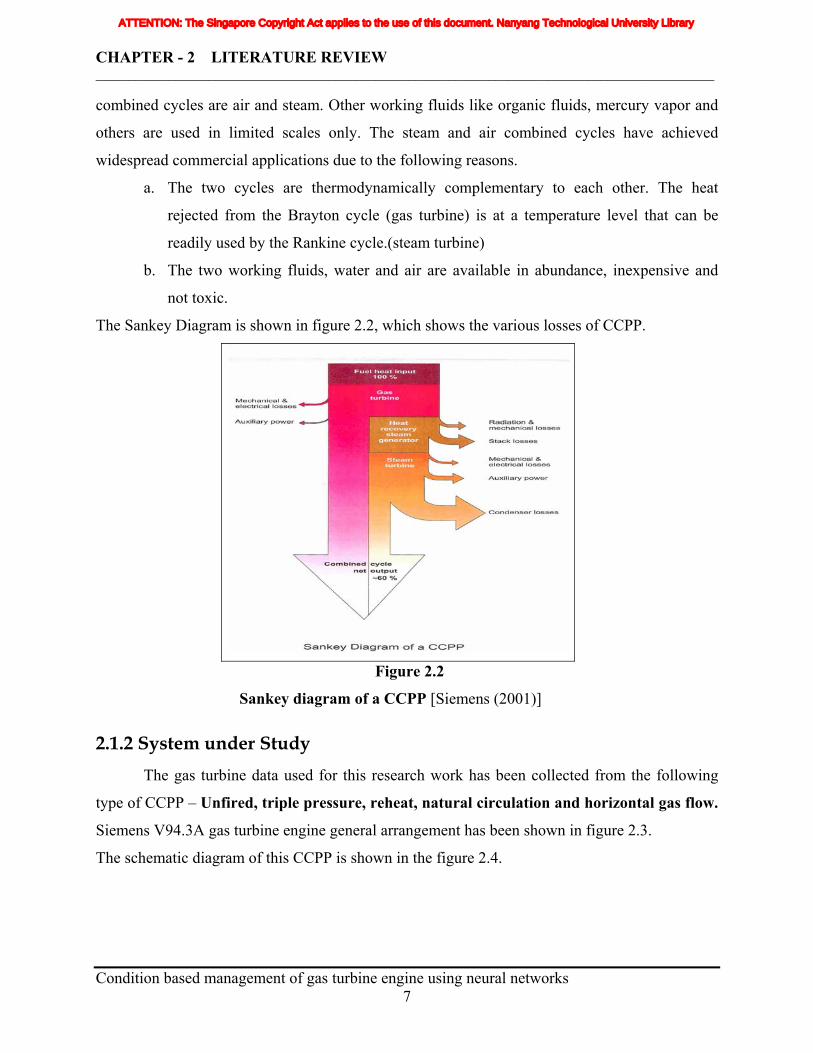
The Sankey Diagram is shown in figure 2.2, which shows the various losses of CCPP.
Figure 2.2
Sankey diagram of a CCPP [Siemens (2001)] 2.1.2 System under Study
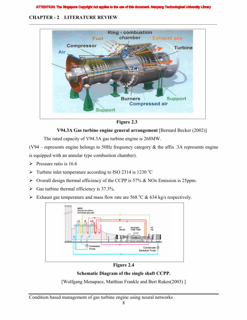
The gas turbine data used for this research work has been collected from the following
type of CCPP – Unfired, triple pressure, reheat, natural circulation and horizontal gas flow.
Siemens V94.3A gas turbine engine general arrangement has been shown in figure 2.3.
The schematic diagram of this CCPP is shown in the figure 2.4.
Condition based management of gas turbine engine using neural networks
7
ATTENTION: The Singapore Copyright Act applies to the use of this document. Nanyang Technological University Library
CHAPTER - 2 LITERATURE REVIEW _____________________________________________________________________________________________
Figure 2.3
V94.3A Gas turbine engine general arrangement [Bernard Becker (2002)]
The rated capacity of V94.3A gas turbine engine is 268MW.
(V94 – represents engine belongs to 50Hz frequency category & the affix .3A represents engine
is equipped with an annular type combustion chamber).
Pressure ratio is 16.6
Turbine inlet temperature according to ISO 2314 is 1230 οC
Overall design thermal efficiency of the CCPP is 57% & NOx Emission is 25ppm.
Gas turbine thermal efficiency is 37.3%.
Exhaust gas temperature and mass flow rate are 568 οC & 634 kg/s respectively.
Figure 2.4
Schematic Diagram of the single shaft CCPP.
[Wolfgang Menapace, Matthias Frankle and Bert Rukes(2003) ]
Condition based management of gas turbine engine using neural networks
8
ATTENTION: The Singapore Copyright Act applies to the use of this document. Nanyang Technological University Library
CHAPTER - 2 LITERATURE REVIEW _____________________________________________________________________________________________
2.2 Classification of gas turbine degradation The degradation of the gas turbine is mainly classified into following types
Recoverable degradation.
Non-recoverable degradation.
Operational degradation.
Recoverable degradation
Degradation that can be recovered through compressor water washing, filter changes,
instrument calibration and auxiliary equipments.
Non- recoverable degradation
Degradation that cannot be recovered through the above methods like compressor
washing, etc is called non-recoverable degradation. But they may be partly recovered through
casing cover lift and refurbishment like changing the seal ring clearances etc.
Operational Degradation
The operational degradation is the sum of the recoverable and non-recoverable degradation.
2.3 Compressor fouling and cleaning The main focus of this research work is to find the effect of compressor fouling in the
performance of the gas turbine. The following section gives introduction about the fouling
phenomenon of compressor, factors contributing the fouling and various cleaning methods
available.
2.3.1 Compressor fouling phenomenon One of the most common problems experienced in the gas turbine engine is the
compressor fouling. Although this problem is not a typical destructive failure, it leads to large
reduction in power output of the gas turbine engine. If left unchecked, it would also lead to
premature hot section component erosion and premature failure of combustor liners etc.
Despite the use of an efficient inlet filter, normal operation of a gas turbine will result in
the accumulation of deposits on the compressor airfoils and gas path passages. This fouling is
caused by the airborne particles such as dirt, sand, industrial chemicals, oil, insects and salts. It
Condition based management of gas turbine engine using neural networks
9
ATTENTION: The Singapore Copyright Act applies to the use of this document. Nanyang Technological University Library

CHAPTER - 2 LITERATURE REVIEW _____________________________________________________________________________________________
alters the air profile and increases the surface roughness. Fouling results in degradation of inlet
flow, compressor efficiency and a reduced compressor surge margin.
The degree of fouling is dependent on the site-specific factors like type and quantity of
the airborne particles, airfoil coatings and ambient conditions. For example, evidence suggests
that high humidity significantly increase the fouling rate. In general, the gas turbine power output
without any compressor washing can be expected to degrade between 2% to 5% after 1000
operating hours. In the combined cycle plants, hot gas mass flow rate degradation outweighs the
exhaust temperature increase and increases the degradation rate of the plant. [Jean-Pierre Stalder
(1998)]
2.3.2 Factors causing fouling The cause of fouling and fouling rates of axial gas turbine compressor is a combination of
various factors that can be classified into following categories.
Gas turbine design parameters.
Site location and surrounding environment.
Plant design and layout.
Atmospheric parameters.
Plant maintenance.
2.3.2.1 Gas turbine design parameters
Smaller engines are highly sensitivity to fouling, when compared to the larger engines.
The degree of the particle deposition on blades increases with growing angle of attack. Further,
the sensitivity to fouling also increases with increasing stage head. Multi-shaft engines are more
sensitive to fouling than single shaft engines. Design parameters such as air inlet velocity at the
inlet guide vanes (IGV), compressor pressure ratio, aerodynamic and geometrical characteristics
will determine the inherent sensitivity to fouling for a specific compressor design.
2.3.2.2 Site location and surrounding environment
Condition based management of gas turbine engine using neural networks
10
The geographical area, the climatic condition, the geological plant location and its
surrounding environment are major factors influencing compressor fouling. These areas can be
classified into desert, tropical, offshore, on-shore, rural, urban and industrial site locations. The
ATTENTION: The Singapore Copyright Act applies to the use of this document. Nanyang Technological University Library
CHAPTER - 2 LITERATURE REVIEW _____________________________________________________________________________________________
expected air borne contaminants (dust, aerosols), their nature (salts, heavy metals etc.),
concentration, particle sizes, weight distribution and climatic conditions are the important
parameters influencing the rate and type of deposition.
2.3.2.3 Plant design and layout
Predominant wind directions can dramatically affect the compressor fouling type and
rates. Orientation and elevation of air inlet / suction must be considered together with the
location of air or water cooling towers in a combined cycle plant. The possibility of exhaust gas
re-circulation into the air inlet, orientation of exhaust pipes from lube-oil tank vapour extractors,
as well as with other local and specific sources of contaminants such as location of highways,
industries, sea shores, etc. should be carefully considered.
Other plant design parameters that affect the rate of compressor fouling are the selection
of air inlet filtration system (self cleaning, depth loading, cell- pocket and oil bath filter, etc.), the
selection of filter media, the number of filtration stages, weather louvers, mist separators,
coalescer, snow hoods, etc. Design parameters such as air velocity through the filters and their
behavior under high humidity condition, pressure drops, etc play critical role in deciding the
fouling nature of the engine. In case, if the conditioning systems are used, then appropriate mist
eliminators should have been installed at the downstream of evaporative coolers. Inlet chilling in
humid areas would result in continuos saturated conditions in the downstream. Thus, the
presence of dust contamination in the air can combine with the moisture and additionally
contribute to compressor fouling. [Jean-Pierre Stalder (1998)]
2.3.2.4 Plant maintenance
Quality of air filtration system maintenance, frequency of compressor blade washing, (the
deposition leads to higher surface blade roughness which in turn leads to faster rate of
degradation), can positively influence compressor fouling and its rate.
2.3.2.5 Atmospheric parameters
Ambient temperature, relativity humidity (dry and wet bulb temperatures), wind forces,
wind direction, precipitation, fog, smog, or mist condition and atmospheric suspend dust
Condition based management of gas turbine engine using neural networks
11
ATTENTION: The Singapore Copyright Act applies to the use of this document. Nanyang Technological University Library
CHAPTER - 2 LITERATURE REVIEW _____________________________________________________________________________________________
concentration related to air density are the parameters having very high impact on the rate of
compressor fouling.
2.3.2.6 Fouling deposits
Most fouling deposits are mixtures of water wettable, water-soluble and water insoluble
materials. Very often pH of 4 and lower can be measured in compressor blade deposits. This
represents risk of pitting corrosion. These deposits become more difficult to remove if left
untreated. The aging process bonds them more firmly to the airfoil surfaces and results in the
reduction of cleaning efficiency. [Jean-Pierre Stalder (1998)]
Water-soluble compounds are hygroscope in nature. These compounds also contain
chlorides, which promotes the pitting corrosion of the compressor blades. Water insoluble
compounds are mostly organic in nature, such as hydrocarbon residues or from silica (Si). These
compounds are quite hard to remove.
2.3.3 Compressor cleaning process In early days, the gas turbine cleaning has been done by crank soak washing and by
injecting solid compounds such as nutshells or rice husks at full speed with the unit in operation.
This method of on-line cleaning by soft erosion has mainly been replaced by wet cleaning due to
the introduction of coated compressor blades. Further unburned solid cleaning compounds and
ashes may also cause blockage of sophisticated turbine blade cooling systems. In the beginning
of 80's, the combination of compressor on-line washings and off-line washings became popular
in the industries. It is found that 5% airflow reduction due to fouled compressor blades leads to a
reduction of power output by 13% and increases heat rate by 5.5%.[Jean-Pierre Stalder (1998)]
The gas turbine compressor washing has gained increasing attention by the owners due to large
scale use of gas turbines in the combined cycle base load application and the increase of their
nominal output. The typical effect of compressor on-line and off-line washing (crank washing)
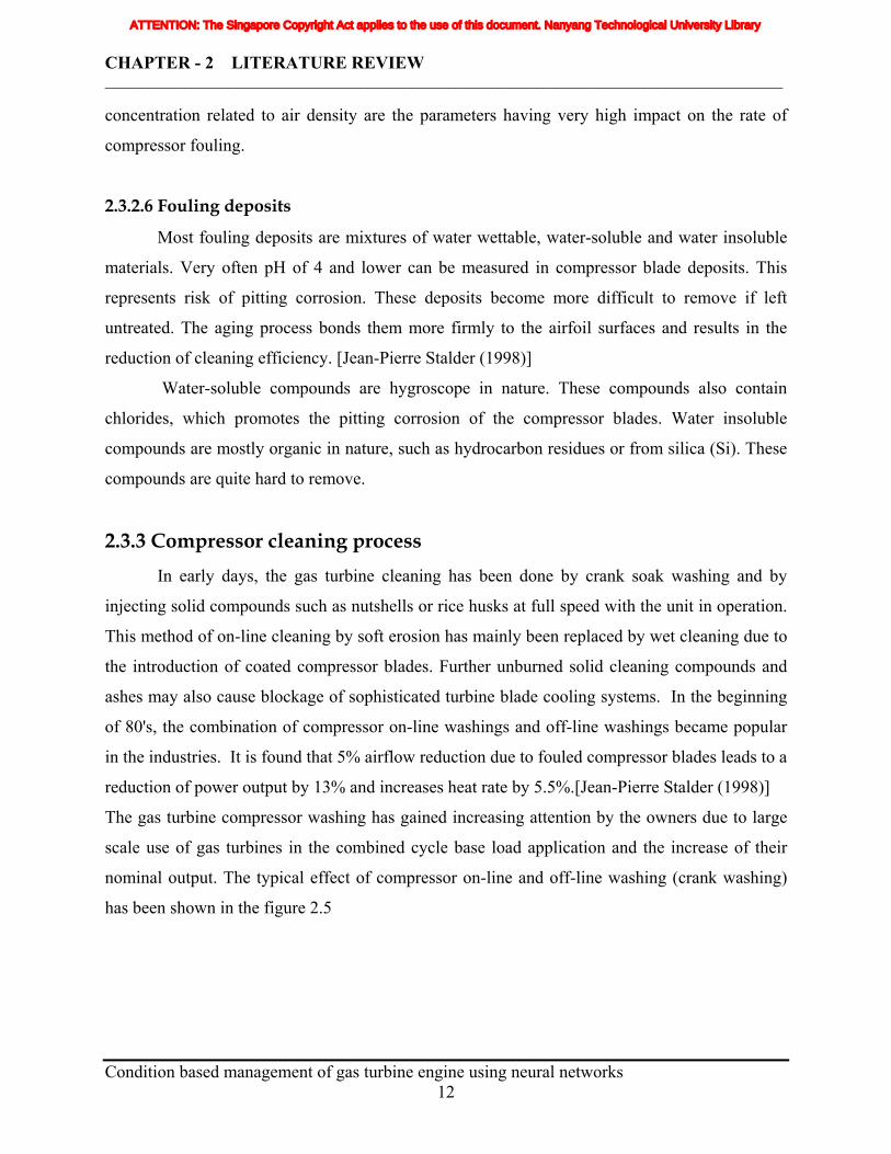
has been shown in the figure 2.5
Condition based management of gas turbine engine using neural networks
12
ATTENTION: The Singapore Copyright Act applies to the use of this document. Nanyang Technological University Library
CHAPTER - 2 LITERATURE REVIEW _____________________________________________________________________________________________
Figure 2.5
Typical effect of on line and off line compressor wet cleaning
[Roemer, M.J and Kacprzynski G.J (2001)]
Three different types of compressor cleaning methods are
a. Dry-cleaning.
b. Off-line washing.
c. On-line washing.
2.3.3.1 Dry-cleaning
Dry cleaning employs the use of nutshells or rice as an abrasive media to scour the
compressor surfaces. This method is rarely used today due to major drawbacks such as the
erosion of airfoils, blade coatings and the plugging of turbine blade cooling holes.
2.3.3.2 Off-line washing
Off-line washing is established as the most effective cleaning method. Crank soaking
with a cleaning fluid mixture allows the removal of deposits from all the compressor stages. The
off-line washing procedure typically involves the injection of a cleaning solution for 15 minutes
at crank speed, followed by a 20 minutes soaking and then thorough rinsing with de-mineralized
water.
The off-line washing method reduces the centrifugal forces on the injected solution. It
leads to better wetting and distribution of the cleaning solution over the blades and vane surfaces
of all the stages. Conductivity and turbidity measurement of the rinsing water will help to assess
the cleaning efficiency. The offline washing nozzles are designed to provide higher mass flow of
bigger droplets. Normally they are known as jet nozzles. Condition based management of gas turbine engine using neural networks
13
ATTENTION: The Singapore Copyright Act applies to the use of this document. Nanyang Technological University Library
CHAPTER - 2 LITERATURE REVIEW _____________________________________________________________________________________________
2.3.3.3 On-line washing
On-line washing is not a replacement to off-line washing. On-line washing can
significantly decrease the fouling rate and maintain performance levels over an extended period
of time. In addition to improving efficiency and heat rate, steady on-line washing can extend the
period between the off-line washings. The on-line washing procedure typically includes the
injection of a cleaning solution for 15 minutes followed by a de-mineral water rinse for at least
15 minutes. [Jean-Pierre Stalder (1998).]
The profiles of the first stage vane play critical roles in deciding the airflow rate through
the gas turbine compressor. The effects of fouling on this first stage vanes are primarily
responsible for a significant reduction of the air mass flow through the compressor, which in turn
reduces the power output. The on-line washing is most effective in removing the deposits on the
first two or three compressor stages. These stages tend to be most heavily fouled. The higher
flow velocities in downstream stages minimize the adhering of deposits.
Droplets of cleaning solution may survive up to the 6th stage, after the 6th stage most of
them get vaporized and the residue/ashes will be centrifuged along the compressor casing.
Therefore, no cleaning solution will be required for removing deposits on downstream stages. A
key element in effective on-line cleaning is the nozzle system. A sufficient number of properly
oriented nozzles are required to create a spray pattern with uniform coverage. The droplets must
be small enough in such way that it would not cause any blade erosion and light enough so as not
to be dropped out of the air stream prematurely.
2.3.4 General compressor cleaning practices The performance degradation of the compressor has high financial impact on the power
plant operation. Therefore maintaining a clean compressor is a high priority task in all gas
turbine power plants. The fouling effects vary from site to site depending on their specific site
conditions. Every site has its own solution in terms of the type and frequency of washing.
Experimentation with good performance monitoring technique is really the best way to optimize
a wash program. [Jean-Pierre Stalder (1998).]
In general, base loaded units should be off-line washed whenever the plant comes down
for maintenance. On-line cleaning with a detergent mixture should be employed 3-4 times per
week followed by a de-mineral water rinsing. Depending on the resulting rate of fouling, an Condition based management of gas turbine engine using neural networks
14
ATTENTION: The Singapore Copyright Act applies to the use of this document. Nanyang Technological University Library
CHAPTER - 2 LITERATURE REVIEW _____________________________________________________________________________________________
economic decision will need to be made whether additional shutdown for off-line crank washing
is required or not. Moderate hour dispatch plants should generally be off-line washed monthly.
Low hour peak plants should be off line washed quarterly. In addition to restoring the full
performance capacity, the washing also removes any salt or other potentially corrosive deposits
from the blade surface and saves the compressor blades.
2.4 Effects of various ambient factors on the combined cycle performance The Combined cycle performance depends not only on component degradation but also
on ambient condition, load level, fuel type and specific installation hardware such as inlet and
outlet ducting. In order to identify the real components degradation the performance monitoring
system must have a correction methodology. The methodology should correct the data to
reference ambient condition and then it could be used for comparison with the baseline data. The
overall gas turbine performance is normally referred to standard inlet conditions of gas turbine
compressor inlet temperature, pressure and relative humidity of 1.01325bar, 15°C and 60%RH.
The referred or corrected parameters take the values that the basic parameters would have at ISA
sea level static conditions. This section explains the details about the effect of various ambient
factors on the gas turbine engine performance and methods to correct the engine performance to
the reference ambient conditions. [John W. Sawyer (1985)].
2.4.1 Effect of various ambient factors on the gas turbine performance Typical forms of curves expressing the dependence of the gas turbine performance on the
ambient conditions have been shown from Figure 2.6 to 2.11. Each gas turbine has its own
curves based on their cycle parameters, component efficiency and mass flow rates. The curves
shown in figure 2.6 to 2.11 are only sample of such curves. These curves are usually used to
determine the values of correction factors for converting the actual performance of gas turbine
from the actual condition to the reference condition. Since they represent the relatively small
deviations around a certain operating condition their form is almost linear. The behavior of the
gas turbine over its entire operating range includes non-linear parameter interrelations. So, one
set of curves is valid only for operating conditions in the vicinity of one load setting. Normally
the set of curves are available for each major load settings like 50%, 75% and 100%.
Condition based management of gas turbine engine using neural networks
15
ATTENTION: The Singapore Copyright Act applies to the use of this document. Nanyang Technological University Library
CHAPTER - 2 LITERATURE REVIEW _____________________________________________________________________________________________
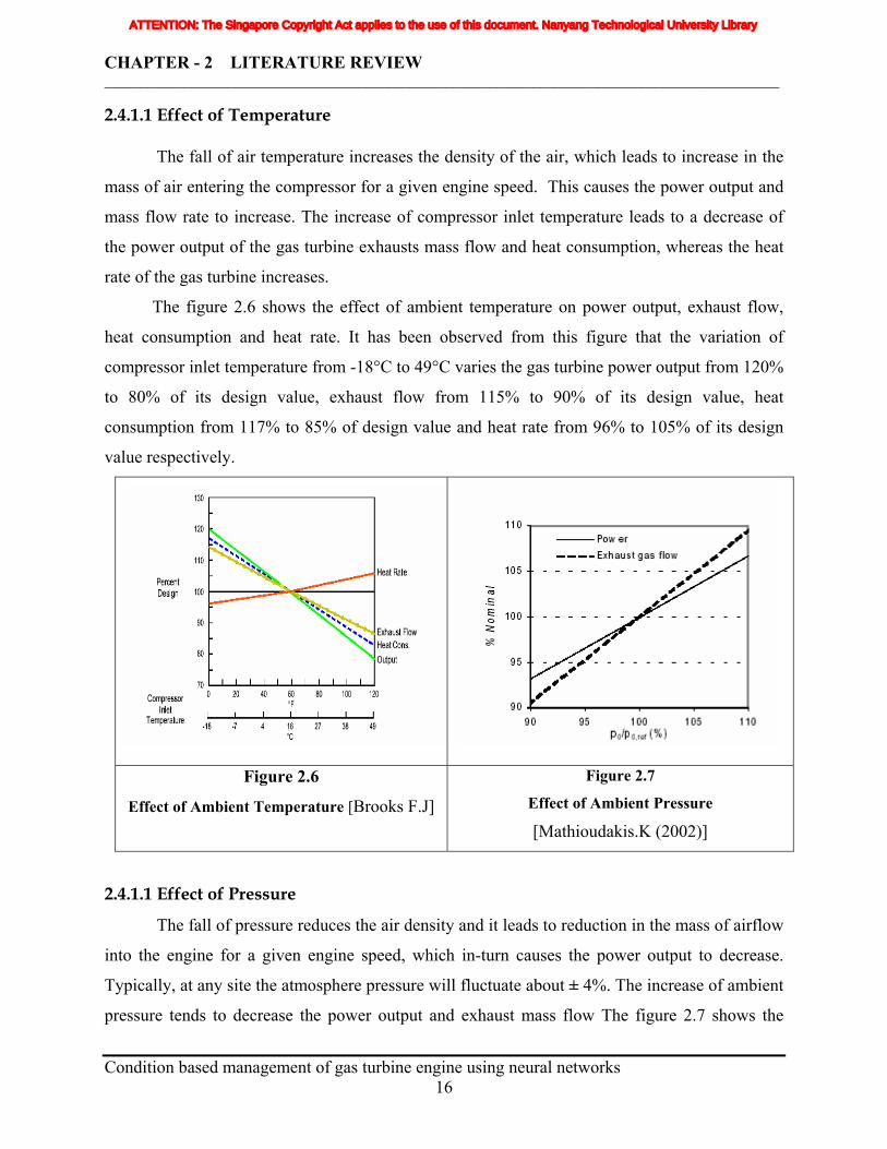
2.4.1.1 Effect of Temperature
The fall of air temperature increases the density of the air, which leads to increase in the
mass of air entering the compressor for a given engine speed. This causes the power output and
mass flow rate to increase. The increase of compressor inlet temperature leads to a decrease of
the power output of the gas turbine exhausts mass flow and heat consumption, whereas the heat
rate of the gas turbine increases.
The figure 2.6 shows the effect of ambient temperature on power output, exhaust flow,
heat consumption and heat rate. It has been observed from this figure that the variation of
compressor inlet temperature from -18°C to 49°C varies the gas turbine power output from 120%
to 80% of its design value, exhaust flow from 115% to 90% of its design value, heat
consumption from 117% to 85% of design value and heat rate from 96% to 105% of its design
value respectively.
Figure 2.6
Effect of Ambient Temperature [Brooks F.J]
Figure 2.7
Effect of Ambient Pressure
[Mathioudakis.K (2002)]
2.4.1.1 Effect of Pressure
The fall of pressure reduces the air density and it leads to reduction in the mass of airflow
into the engine for a given engine speed, which in-turn causes the power output to decrease.
Typically, at any site the atmosphere pressure will fluctuate about ± 4%. The increase of ambient
pressure tends to decrease the power output and exhaust mass flow The figure 2.7 shows the
Condition based management of gas turbine engine using neural networks
16
ATTENTION: The Singapore Copyright Act applies to the use of this document. Nanyang Technological University Library
CHAPTER - 2 LITERATURE REVIEW _____________________________________________________________________________________________
effect of ambient pressure on the exhaust gas flow and power output. It has been observed from
figure 2.7, the variation of ambient pressure (p0/p0ref) of about 90% to 110% from its rated ISO
condition varies the power output from 90% to 110% and exhaust gas mass flow from 94% to
106% of its design values respectively. The heat rate and other cycle parameters are not affected
by ambient pressure variation.
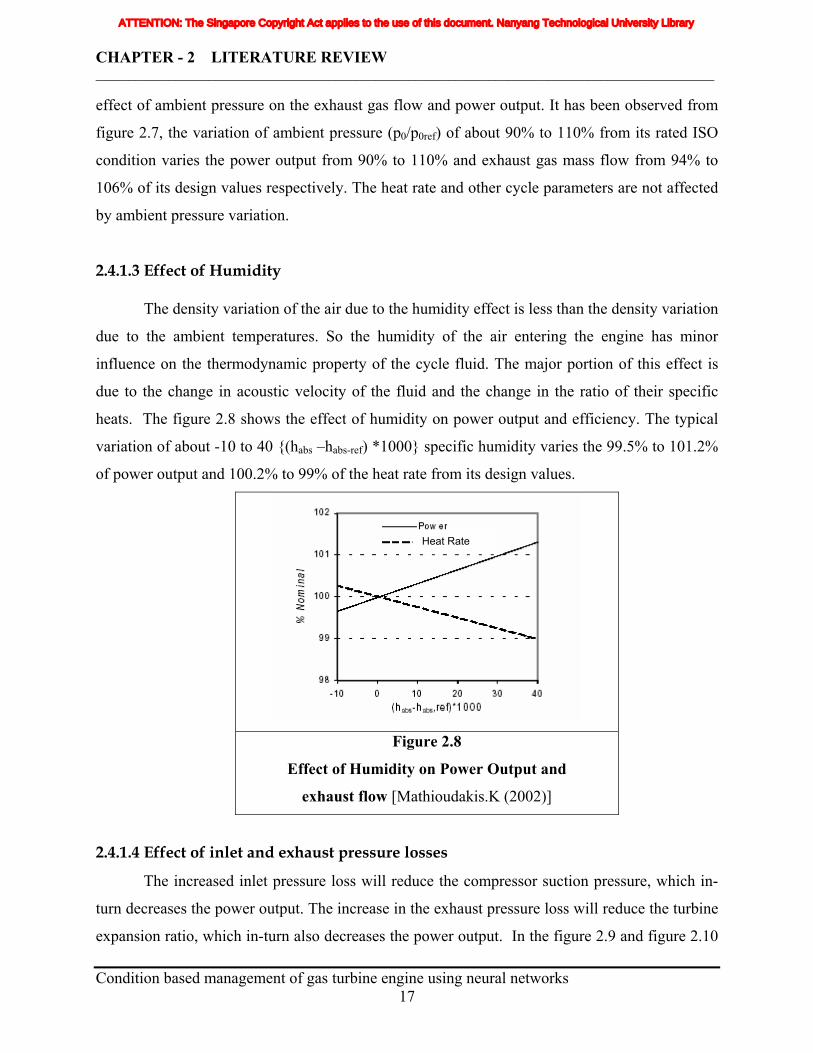
2.4.1.3 Effect of Humidity
The density variation of the air due to the humidity effect is less than the density variation
due to the ambient temperatures. So the humidity of the air entering the engine has minor
influence on the thermodynamic property of the cycle fluid. The major portion of this effect is
due to the change in acoustic velocity of the fluid and the change in the ratio of their specific
heats. The figure 2.8 shows the effect of humidity on power output and efficiency. The typical
variation of about -10 to 40 {(habs –habs-ref) *1000} specific humidity varies the 99.5% to 101.2%
of power output and 100.2% to 99% of the heat rate from its design values.
Figure 2.8
Effect of Humidity on Power Output and
exhaust flow [Mathioudakis.K (2002)]
Heat Rate
2.4.1.4 Effect of inlet and exhaust pressure losses
The increased inlet pressure loss will reduce the compressor suction pressure, which in-
turn decreases the power output. The increase in the exhaust pressure loss will reduce the turbine
expansion ratio, which in-turn also decreases the power output. In the figure 2.9 and figure 2.10 Condition based management of gas turbine engine using neural networks
17
ATTENTION: The Singapore Copyright Act applies to the use of this document. Nanyang Technological University Library
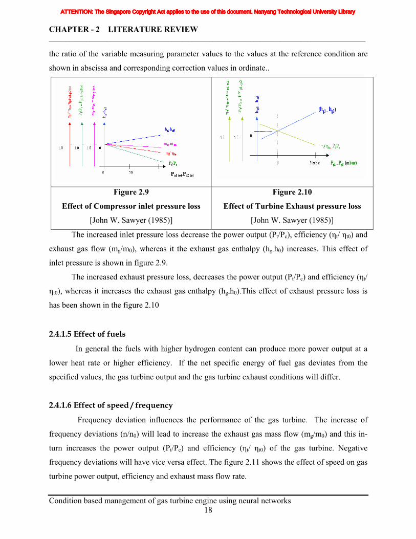
CHAPTER - 2 LITERATURE REVIEW _____________________________________________________________________________________________
the ratio of the variable measuring parameter values to the values at the reference condition are
shown in abscissa and corresponding correction values in ordinate..
Figure 2.9
Effect of Compressor inlet pressure loss
[John W. Sawyer (1985)]
Figure 2.10
Effect of Turbine Exhaust pressure loss
[John W. Sawyer (1985)]
The increased inlet pressure loss decrease the power output (Pt/Pc), efficiency (ηt/ ηt0) and
exhaust gas flow (mg/m0), whereas it the exhaust gas enthalpy (hg-h0) increases. This effect of
inlet pressure is shown in figure 2.9.
The increased exhaust pressure loss, decreases the power output (Pt/Pc) and efficiency (ηt/
ηt0), whereas it increases the exhaust gas enthalpy (hg-h0).This effect of exhaust pressure loss is
has been shown in the figure 2.10
2.4.1.5 Effect of fuels
In general the fuels with higher hydrogen content can produce more power output at a
lower heat rate or higher efficiency. If the net specific energy of fuel gas deviates from the
specified values, the gas turbine output and the gas turbine exhaust conditions will differ.
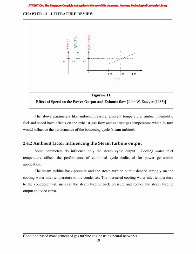
2.4.1.6 Effect of speed / frequency
Frequency deviation influences the performance of the gas turbine. The increase of
frequency deviations (n/n0) will lead to increase the exhaust gas mass flow (mg/m0) and this in-
turn increases the power output (Pt/Pc) and efficiency (ηt/ ηt0) of the gas turbine. Negative
frequency deviations will have vice versa effect. The figure 2.11 shows the effect of speed on gas
turbine power output, efficiency and exhaust mass flow rate.
Condition based management of gas turbine engine using neural networks
18
ATTENTION: The Singapore Copyright Act applies to the use of this document. Nanyang Technological University Library
CHAPTER - 2 LITERATURE REVIEW _____________________________________________________________________________________________
Figure-2.11
Effect of Speed on the Power Output and Exhaust flow [John W. Sawyer (1985)]
The above parameters like ambient pressure, ambient temperature, ambient humidity,
fuel and speed have effects on the exhaust gas flow and exhaust gas temperature which in turn
would influence the performance of the bottoming cycle (steam turbine).
2.4.2 Ambient factor influencing the Steam turbine output Some parameters do influence only the steam cycle output. Cooling water inlet
temperature affects the performance of combined cycle dedicated for power generation
application.
The steam turbine back-pressure and the steam turbine output depend strongly on the
cooling water inlet temperature to the condenser. The increased cooling water inlet temperature
to the condenser will increase the steam turbine back pressure and reduce the steam turbine
output and vice versa.
Condition based management of gas turbine engine using neural networks
19
ATTENTION: The Singapore Copyright Act applies to the use of this document. Nanyang Technological University Library

CHAPTER - 2 LITERATURE REVIEW _____________________________________________________________________________________________
2.5 Correction of test results to reference conditions The Gas turbine performance is highly influenced by the ambient parameters like intake
air's (inlet air) temperature, pressure, humidity and also other factors like speed, calorific value
of fuel etc. These parameters are variable with respect to time and other factors. (e.g. with lower
ambient temperature and higher fuel calorific value, gas turbine can produce more power output
and vice versa). It is wrong to do the direct comparison of the engine performance monitoring
parameters under various conditions. It is also not always possible to run the engine at the
specified reference or standard conditions. So, the results of the engine performance monitoring
parameters have to be corrected to the reference conditions to facilitate their comparison at
various conditions. The following paragraph gives the details about various techniques available
for the correction of test result to the reference conditions. [ Walsh (1998)]
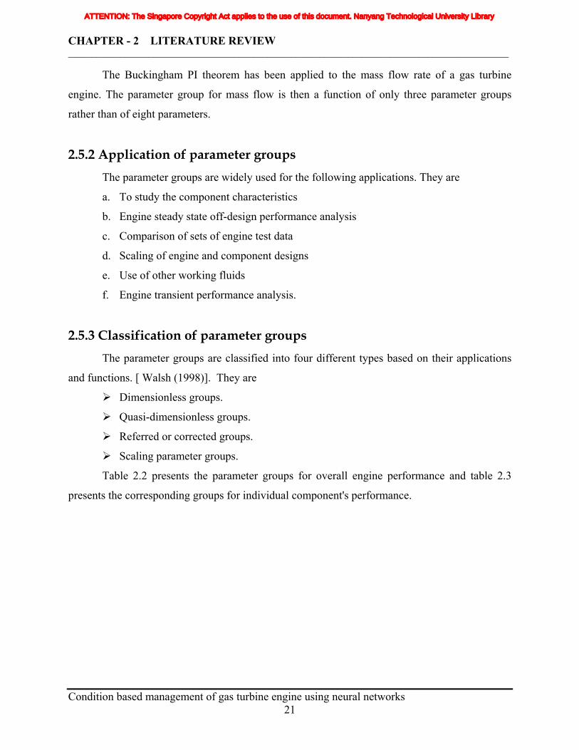
2.5.1 Importance of parameter groups Large number of variables is required to numerically describe the engine performance
throughout the operational envelopes. The Bunkingham PI theorem reduces the large number of
parameters to a small number of dimensionless parameter groups. In these groups, the
parameters are multiplied together and each is raised to some exponent. The result greatly
simplifies the understanding and graphical representation of engine performance. For instance,
the steady state mass flow rate of a turbojet engine is a function of eight parameters as shown in
the table 2.1
SN Inlet mass flow is a function of SN Dimensionless group for inlet mass flow is a function of
1 Ambient temperature 2 Ambient pressure
1 Dimensionless group for engine speed
3 Flight Mach number 2 Flight Mach number 4 Engine rotational speed 5 Engine diameter 6 Gas constant of working fluid 7 Gamma for working fluid 8 Viscosity of working fluid
3 Dimensionless group for viscosity (has only a second-order effect, and is often ignored for initial calculations)
Table 2.1
Conversion of normal parameters to Dimensionless groups
Condition based management of gas turbine engine using neural networks
20
ATTENTION: The Singapore Copyright Act applies to the use of this document. Nanyang Technological University Library
CHAPTER - 2 LITERATURE REVIEW _____________________________________________________________________________________________
The Buckingham PI theorem has been applied to the mass flow rate of a gas turbine
engine. The parameter group for mass flow is then a function of only three parameter groups
rather than of eight parameters.
2.5.2 Application of parameter groups The parameter groups are widely used for the following applications. They are
a. To study the component characteristics
b. Engine steady state off-design performance analysis
c. Comparison of sets of engine test data
d. Scaling of engine and component designs
e. Use of other working fluids
f. Engine transient performance analysis.
2.5.3 Classification of parameter groups The parameter groups are classified into four different types based on their applications
and functions. [ Walsh (1998)]. They are
Dimensionless groups.
Quasi-dimensionless groups.
Referred or corrected groups.
Scaling parameter groups.
Table 2.2 presents the parameter groups for overall engine performance and table 2.3
presents the corresponding groups for individual component's performance.
Condition based management of gas turbine engine using neural networks
21
ATTENTION: The Singapore Copyright Act applies to the use of this document. Nanyang Technological University Library
CHAPTER - 2 LITERATURE REVIEW _____________________________________________________________________________________________
Performance parameter
Dimensionless Group
Quasi-dimensionless
Group
Referred parameter
Scaling parameter
1 Temperature at station n (Tn)
Cp x(Tn/T1 –1) γ x R
Tn/ T1 or TSn/T1 Tn/θ or TSn/θ Tn/θ or TSn/θ
2 Pressure at station n (Pn)
Cp x(Pn/P1(γ-1) / γ –1) γ x R
Pn/ P1 or PSn/P1 Pn/δ or PSn/δ Pn/δ or PSn/δ
3 Mass flow (W) W x √(T1 x R) DI2x P1* √( γ)
W x √(T1) P1
W x √( θ) δ
W x √( θ) DI2 x δ
4 Rotational Speed (N)
N x DI √( γ x R x T)
N / √( T1) N / √( θ) (DI x N) / √( θ)
5 Fuel Flow(WF) WF x FHVx √(R) x ETA31 CP x DI2 x PI x √( T1 x γ )
WF x FHV x ETA31 PI x √( T1 )
WF x FHV x ETA31 δ x √( θ )
WF x FHV x ETA31
DI2 x δ x √( θ )
6 Fuel air ratio (FAR)
FAR x FHV x ETA31 Cp x T1
FAR x FHV x ETA31 T1
FAR x FHV x ETA31 √( θ)
FAR x FHV x ETA31 √( θ)
7 Shaft power (PW)
PW γ x DI2 x P1 x √( γ x
R x T1 )
PW PI x √( T1)
PW δ x √( θ )
PW DI2 x δ x √( θ )
8 Shaft power SFC (SFC)
SFC x FHV x γ x R x ETA31
Cp
SFC x FHV x ETA31 SFC x FHV x ETA31
SFC x FHV x ETA31
9 Shaft specific power (SPW)
SPW γ x R x T1
SPW / T1 SPW / θ SPW / θ
10 Gross thrust (FG)
FG γ x DI2 x P1
FG / P1 FG / δ FG / ( DI2 x δ)
11 Momentum drag (FRAM)
FRAM γ x DI2 x P1
FRAM / P1 FRAM / δ FRAM / ( DI2 x δ)
12 Gross thrust parameter (FG)
FG / (A9 x PAMB) +1 γ x DI2 x P1/ (PAMB)
FG / (A9 x PAMB) +1 P1/ (PAMB)
FG / (A9 x PAMB) +1
P1/ (PAMB)
FG / (A9 x PAMB) +1
DI2 x P1/ (PAMB) 13 Thrust (SFC) SFC x FHV x √( γ x
R) x ETA31 CP x √ (T1)
SFC x FHV x ETA31 √ (T1)
SFC x FHV x ETA31 √ (θ)
SFC x FHV x ETA31 √ (θ)
14 Specific thrust (SFG)
SFG √( γ x R x T1 )
SFG / √ (T1)
SFG / √ (θ ) SFG / √ (θ )
15 Gas velocity at station n (Vn)
Vn √( γ x R x T1 )
Vn / √ (T1)
Vn / √ (θ ) Vn / √ (θ )
16 Density at station n (RHOn)
RHOn x R x T1 / P1 RHOn x T1 / P1 RHOn x θ / δ RHOn x θ / δ
Table 2.2
Engine Parameter Groups [Walsh (1998)]
Condition based management of gas turbine engine using neural networks
22
ATTENTION: The Singapore Copyright Act applies to the use of this document. Nanyang Technological University Library
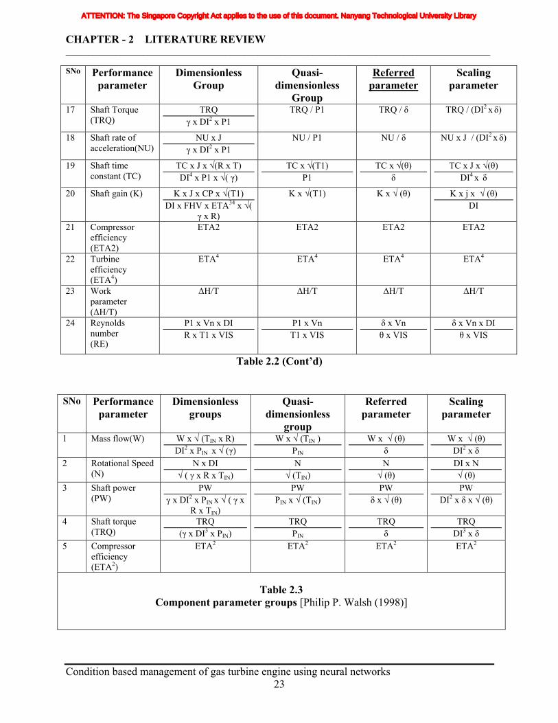
CHAPTER - 2 LITERATURE REVIEW _____________________________________________________________________________________________
SNo Performance parameter
Dimensionless Group
Quasi-dimensionless
Group
Referred parameter
Scaling parameter
17 Shaft Torque (TRQ)
TRQ γ x DI2 x P1
TRQ / P1 TRQ / δ TRQ / (DI2 x δ)
18 Shaft rate of acceleration(NU)
NU x J γ x DI2 x P1
NU / P1 NU / δ NU x J / (DI2 x δ)
19 Shaft time constant (TC)
TC x J x √(R x T) DI4 x P1 x √( γ)
TC x √(T1) P1
TC x √(θ) δ
TC x J x √(θ) DI4 x δ
20 Shaft gain (K) K x J x CP x √(T1) DI x FHV x ETA34 x √(
γ x R)
K x √(T1) K x √ (θ) K x j x √ (θ) DI
21 Compressor efficiency (ETA2)
ETA2 ETA2 ETA2 ETA2
22 Turbine efficiency (ETA4)
ETA4 ETA4 ETA4 ETA4
23 Work parameter (∆H/T)
∆H/T ∆H/T ∆H/T ∆H/T
24 Reynolds number (RE)
P1 x Vn x DI R x T1 x VIS
P1 x Vn T1 x VIS
δ x Vn θ x VIS
δ x Vn x DI θ x VIS
Table 2.2 (Cont’d)
SNo Performance parameter
Dimensionless groups
Quasi-dimensionless
group
Referred parameter
Scaling parameter
1 Mass flow(W) W x √ (TIN x R) DI2 x PIN x √ (γ)
W x √ (TIN ) PIN
W x √ (θ) δ
W x √ (θ) DI2 x δ
2 Rotational Speed (N)
N x DI √ ( γ x R x TIN)
N √ (TIN)
N √ (θ)
DI x N √ (θ)
3 Shaft power (PW)
PW γ x DI2 x PIN x √ ( γ x
R x TIN)
PW PIN x √ (TIN)
PW δ x √ (θ)
PW DI2 x δ x √ (θ)
4 Shaft torque (TRQ)
TRQ (γ x DI3 x PIN)
TRQ PIN
TRQ δ
TRQ DI3 x δ
5 Compressor efficiency (ETA2)
ETA2 ETA2 ETA2 ETA2
Table 2.3
Component parameter groups [Philip P. Walsh (1998)]
Condition based management of gas turbine engine using neural networks
23
ATTENTION: The Singapore Copyright Act applies to the use of this document. Nanyang Technological University Library
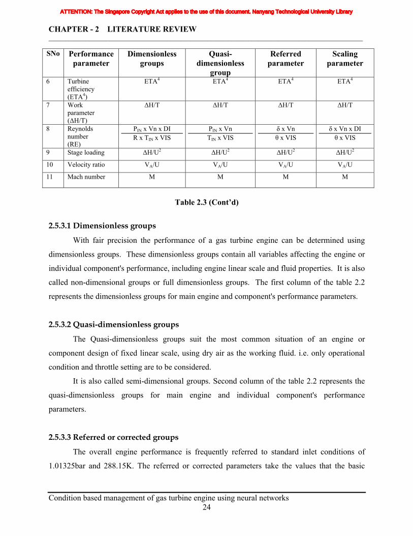
CHAPTER - 2 LITERATURE REVIEW _____________________________________________________________________________________________
SNo Performance parameter
Dimensionless groups
Quasi-dimensionless
group
Referred parameter
Scaling parameter
6 Turbine efficiency (ETA4)
ETA4 ETA4 ETA4 ETA4
7 Work parameter (∆H/T)
∆H/T ∆H/T ∆H/T ∆H/T
8 Reynolds number (RE)
PIN x Vn x DI R x TIN x VIS
PIN x Vn TIN x VIS
δ x Vn θ x VIS
δ x Vn x DI θ x VIS
9 Stage loading ∆H/U2 ∆H/U2 ∆H/U2 ∆H/U2
10 Velocity ratio VA/U VA/U VA/U VA/U
11 Mach number M M M M
Table 2.3 (Cont’d)
2.5.3.1 Dimensionless groups
With fair precision the performance of a gas turbine engine can be determined using
dimensionless groups. These dimensionless groups contain all variables affecting the engine or
individual component's performance, including engine linear scale and fluid properties. It is also
called non-dimensional groups or full dimensionless groups. The first column of the table 2.2
represents the dimensionless groups for main engine and component's performance parameters.
2.5.3.2 Quasi-dimensionless groups
The Quasi-dimensionless groups suit the most common situation of an engine or
component design of fixed linear scale, using dry air as the working fluid. i.e. only operational
condition and throttle setting are to be considered.
It is also called semi-dimensional groups. Second column of the table 2.2 represents the
quasi-dimensionless groups for main engine and individual component's performance
parameters.
2.5.3.3 Referred or corrected groups
The overall engine performance is frequently referred to standard inlet conditions of
1.01325bar and 288.15K. The referred or corrected parameters take the values that the basic
Condition based management of gas turbine engine using neural networks
24
ATTENTION: The Singapore Copyright Act applies to the use of this document. Nanyang Technological University Library
CHAPTER - 2 LITERATURE REVIEW _____________________________________________________________________________________________
parameters would have at ISA sea level static conditions. These parameter groups are directly
proportional to the quasi-dimensionless groups and hence they are interchangeable in usage.
The difference is the substitution of theta (θ) and delta (δ) for engine or component inlet pressure
and temperature, where as
Theta (θ) = inlet temperature / 288.15K
Delta (δ) = inlet pressure/1.01325 bar
The resulting groups are given in the third column of the table 2.2
2.5.3.4 Scaling parameter groups
They are mainly used in the concept design of new engines. The working fluid properties
are omitted in these groups. They are used to quickly access the performance effects of linear
scaling to an existing engine, or matching differentially scaled existing compressor and turbines.
The fourth column of table 2.2 represents the scaling parameter groups for the main engine and
component parameters.
2.5.4 First order effects For a given operational condition, knowledge of the absolute values of inlet pressure and
temperature allows easy calculation of the actual performance parameters. The off-design
performance parameters to a level of first order accuracy are given in the table 2.2 and table 2.3.
These tables show the interrelationship of the referred parameter groups. The value of these
tables cannot be over emphasized. They enable 'on the spot' judgements during engine testing, or
discussing in a meeting the impact of an extreme operating points. The parameter groups account
for the first order approximation of gas turbine engine component characteristics, scaling, steady
state and transient performance evaluation. [ Walsh (1998)]
2.5.5 Second order effects When a rigorous analysis must be pursued then all effects must be fully accounted and
this invariably requires complex computer codes. There are various phenomena that have a
second-order effect upon engine matching, and they will also affect the parameter group
relationships. Although these effects may be ignored, if first-order accuracy is only required.
Condition based management of gas turbine engine using neural networks
25
ATTENTION: The Singapore Copyright Act applies to the use of this document. Nanyang Technological University Library

CHAPTER - 2 LITERATURE REVIEW _____________________________________________________________________________________________
[ Walsh (1998)]. The following examples show the difference of the second order effect with the
first order effect.
Second order effect of Humidity and water or steam injection
The effect of water vapour on engine performance can be significant due to change of gas
properties. To a first order accuracy level, this effect is small and may be neglected. But for a
second order accuracy level this effect has significant influence over gas turbine performances
and it has to be included.
Second order effect of the Inlet and exit conditions
For a given engine design, non-standard inlet and exit conditions may cause the engine to
deviate from its normal non-dimensional behavior. e.g.
a. Different installation inlet and exhaust losses due to change of application filter
blockage etc.
b. Flow distortion at the first compressor inlet due to cross wind or aircraft pitch and yaw.
To a first order accuracy level, these effects are small and may be neglected. But for a
second order accuracy level these effects have significant influence over gas turbine
performances and they have to be included.
The application of parameter groups for analyzing the steady state performance yields the
result to a first order accuracy level, whereas the correction factors specified by the equipment
supplier incorporates the second order effects and they will provide more accurate results.
2.5.6 Correction of test results to the reference conditions for variable
speed gas turbines In case of variable speed characteristics, such as mechanical drive, the corrections shall
be made as follows [ISO 2314:1989(E)]
2.5.6.1 Determination of output shaft test speed (nt)
nt = n0√θ
where n0 is the reference speed and θ is the ratio of the absolute test ambient temperature to the
absolute reference ambient temperature.
Condition based management of gas turbine engine using neural networks
26
ATTENTION: The Singapore Copyright Act applies to the use of this document. Nanyang Technological University Library
CHAPTER - 2 LITERATURE REVIEW _____________________________________________________________________________________________
2.5.6.2 Determination of absolute test temperature (Tt )
Tt = Tθ
where T is the absolute temperature for the reference conditions and θ is the ratio of the absolute
test ambient temperature to the absolute reference ambient temperature.
2.5.6.3 Determination of corrected net shaft power output (Pc )
The net shaft power output Pt may be determined from the measured gross test shaft
output. The corrected net shaft power output, Pc will then be given as follows
Pc= Pt / (δ√θ)
where Pt is the test net shaft power outlet, δ is the ratio of the ambient absolute pressure
to the reference ambient absolute pressure and θ is the ratio of the absolute test ambient
temperature to the absolute reference ambient temperature.
2.5.6.4 Determination of the thermal efficiency (ηt)
The thermal efficiency of the variable speed gas turbine is calculated as follows
ηt = Pt/ (mm *(Ql0+hf4-h0))
where mm is the measured rate of fuel consumption in kilograms per second.
Ql0 is the net specific energy of the fuel at 15°C and constant pressure in kJ/kg.
hf4 is the specific enthalpy of the fuel at temperature Tf4 entering the heat source (combustion
chamber) in kJ/kg and h0 is the specific enthalpy of the fuel at 15°C in kJ/kg.
2.5.7 Correction of test results to the reference conditions for constant
speed gas turbines Correction of test load and thermal efficiency for generator drive or other constant speed
applications is less straightforward, since it is impossible to operate the engine at the same
aerodynamic conditions. Therefore the gas turbine engine would be operating at off design point
whenever the compressor inlet conditions are different from the reference conditions. Every
effort shall be made to run the test at reference conditions. If this is not feasible, then the test will
have to be based on proper correction curves. This corrections include the effect of parameters
influencing load and efficiency including (but not limited to) compressor inlet temperature,
Condition based management of gas turbine engine using neural networks
27
ATTENTION: The Singapore Copyright Act applies to the use of this document. Nanyang Technological University Library
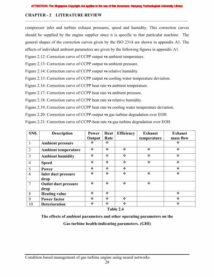
CHAPTER - 2 LITERATURE REVIEW _____________________________________________________________________________________________
compressor inlet and turbine exhaust pressures, speed and humidity. This correction curves
should be supplied by the engine supplier since it is specific to that particular machine. The
general shapes of the correction curves given by the ISO 2314 are shown in appendix A1. The
effects of individual ambient parameters are given by the following figures in appendix A1.
Figure 2.12: Correction curve of CCPP output vs ambient temperature.
Figure 2.13: Correction curve of CCPP output vs ambient pressure.
Figure 2.14: Correction curve of CCPP output vs relative humidity.
Figure 2.15: Correction curve of CCPP output vs cooling water temperature deviation.
Figure 2.16: Correction curve of CCPP heat rate vs ambient temperature.
Figure 2.17: Correction curve of CCPP heat rate vs ambient pressure.
Figure 2.18: Correction curve of CCPP heat rate vs relative humidity.
Figure 2.19: Correction curve of CCPP heat rate vs cooling water temperature deviation.
Figure 2.20: Correction curve of CCPP-output vs gas turbine degradation over EOH
Figure 2.21: Correction curve of CCPP-heat rate vs gas turbine degradation over EOH
SN0. Description Power Output
Heat Rate
Efficiency Exhaust temperature
Exhaust mass flow
1 Ambient pressure
2 Ambient temperature
3 Ambient humidity
4 Speed
5 Power 6 Inlet duct pressure
drop
7 Outlet duct pressure drop
8 Heating value
9 Power factor 10 Deterioration
Table 2.4
The effects of ambient parameters and other operating parameters on the
Gas turbine health-indicating parameters. (GHI)
Condition based management of gas turbine engine using neural networks
28
ATTENTION: The Singapore Copyright Act applies to the use of this document. Nanyang Technological University Library
CHAPTER - 2 LITERATURE REVIEW _____________________________________________________________________________________________
The effect of ambient parameters and the operating parameters like speed and fuel flow
etc on the equipment health indicating parameters like power output, heat rate, efficiency,
exhaust temperature and exhaust gas flow rate are simplified and shown in table 2.4. 2.6 Introduction to the Gas turbine controllers for CCPP
The knowledge about the gas turbine controller plays vital role to understand the
behavior of the gas turbine during various operating conditions. Figure 2.22 shows the concept
of the GT controller for combined cycle plant. The GT controller controls the following
operational states of the gas turbine engine. [Siemens (2001)]
a) Start up.
b) Synchronizing.
c) Loading / unloading.
d) Load limitation and Load rejection.
e) Shutdown.
2.6.1 Various control devices to achieve GT controller Tasks a) Startup / Runup controller.
b) Speed / Load controller
c) Temperature controller.
d) Load limit controller.
e) Lift controllers of fuel oil valves.
Apart from the above controllers, the gas turbine has the following special controllers to
protect the engine from abnormal operations.
f) Compressor outlet pressure gradient limit controller.
g) Compressor pressure ratio limit controller.
h) Compressor discharge temperature limit controller.
Condition based management of gas turbine engine using neural networks
29
ATTENTION: The Singapore Copyright Act applies to the use of this document. Nanyang Technological University Library
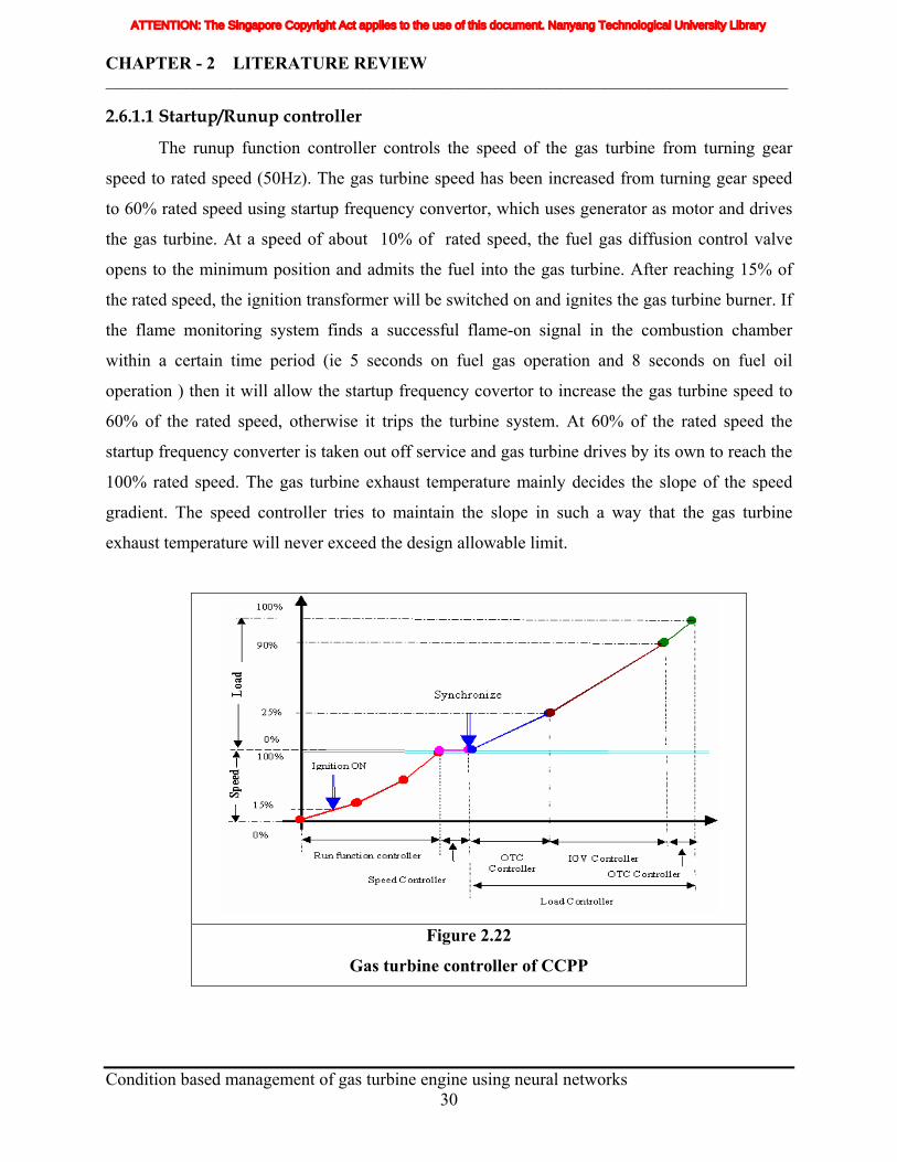
CHAPTER - 2 LITERATURE REVIEW _____________________________________________________________________________________________
2.6.1.1 Startup/Runup controller
The runup function controller controls the speed of the gas turbine from turning gear
speed to rated speed (50Hz). The gas turbine speed has been increased from turning gear speed
to 60% rated speed using startup frequency convertor, which uses generator as motor and drives
the gas turbine. At a speed of about 10% of rated speed, the fuel gas diffusion control valve
opens to the minimum position and admits the fuel into the gas turbine. After reaching 15% of
the rated speed, the ignition transformer will be switched on and ignites the gas turbine burner. If
the flame monitoring system finds a successful flame-on signal in the combustion chamber
within a certain time period (ie 5 seconds on fuel gas operation and 8 seconds on fuel oil
operation ) then it will allow the startup frequency covertor to increase the gas turbine speed to
60% of the rated speed, otherwise it trips the turbine system. At 60% of the rated speed the
startup frequency converter is taken out off service and gas turbine drives by its own to reach the
100% rated speed. The gas turbine exhaust temperature mainly decides the slope of the speed
gradient. The speed controller tries to maintain the slope in such a way that the gas turbine
exhaust temperature will never exceed the design allowable limit.
Figure 2.22
Gas turbine controller of CCPP
Condition based management of gas turbine engine using neural networks
30
ATTENTION: The Singapore Copyright Act applies to the use of this document. Nanyang Technological University Library
CHAPTER - 2 LITERATURE REVIEW _____________________________________________________________________________________________
2.6.1.2 Speed Controller
The speed controller tries to maintain the gas turbine speed by about 1% greater than the
grid speed and allows the auto or manual synchronizing device to do the synchronizing
operation.
2.6.1.3 Load Controller
After synchronizing the machine with the grid, the load controller takes over the speed
controller functions and controls the turbine load. The load controller pre-controls the fuel valve
lift. The load controller thus controls operation over the entire load range from 0% to 100%. The
other controllers like outlet temperature controller (OTC), inlet guide vane controller (IGV) and
load set point determines the function of the load controller.
2.6.1.4 OTC Controller
The turbine inlet temperature cannot be measured directly due to its high range
(i.e. 1250°C), so the turbine outlet temperature is measured by using twenty four thermocouples.
Based on the actual ambient temperature, the average outlet temperature of these twenty four
thermocouples is corrected. This corrected value is fed into the gas turbine controller, which
determines the behavior of the OTC controller. The main function of the OTC controller is to
control the gas flow rate and airflow rate to achieve the following criteria
To maintain the temperature difference between average OTC temperature and main
steam inlet temperature of the HP steam turbine less than 50°C in order to avoid thermal
stress to the boiler HP superheater tubes. (for loads 0% to 25%).
To maintain the average corrected OTC temperature less than 580°C. (for loads >90%).
2.6.1.5 IGV Controller
Once the HRSG outlet steam temperature optimized with the gas turbine exhaust
temperature, (i.e. after reaching a load of about 25%) the gas turbine controller transfers the
control from OTC to IGV controller. The main function of the IGV controller is to control the
airflow rate of the gas turbine compressor and fuel gas flow rate based on the load set point. The
inlet guide vane opening and fuel gas control valve opening are directly proportional to the load
set point, with increase in load set point the openings will be increased and vice versa. OTC of Condition based management of gas turbine engine using neural networks
31
ATTENTION: The Singapore Copyright Act applies to the use of this document. Nanyang Technological University Library
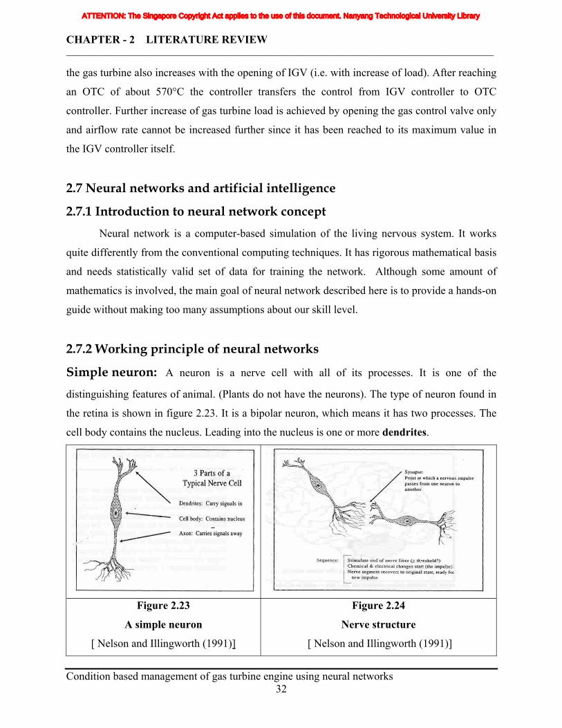
CHAPTER - 2 LITERATURE REVIEW _____________________________________________________________________________________________
the gas turbine also increases with the opening of IGV (i.e. with increase of load). After reaching
an OTC of about 570°C the controller transfers the control from IGV controller to OTC
controller. Further increase of gas turbine load is achieved by opening the gas control valve only
and airflow rate cannot be increased further since it has been reached to its maximum value in
the IGV controller itself.
2.7 Neural networks and artificial intelligence
2.7.1 Introduction to neural network concept Neural network is a computer-based simulation of the living nervous system. It works
quite differently from the conventional computing techniques. It has rigorous mathematical basis
and needs statistically valid set of data for training the network. Although some amount of
mathematics is involved, the main goal of neural network described here is to provide a hands-on
guide without making too many assumptions about our skill level.
2.7.2 Working principle of neural networks
Simple neuron: A neuron is a nerve cell with all of its processes. It is one of the
distinguishing features of animal. (Plants do not have the neurons). The type of neuron found in
the retina is shown in figure 2.23. It is a bipolar neuron, which means it has two processes. The
cell body contains the nucleus. Leading into the nucleus is one or more dendrites.
Condition based management of gas turbine engine using neural networks
32
Figure 2.23
A simple neuron
[ Nelson and Illingworth (1991)]
Figure 2.24
Nerve structure
[ Nelson and Illingworth (1991)]
ATTENTION: The Singapore Copyright Act applies to the use of this document. Nanyang Technological University Library
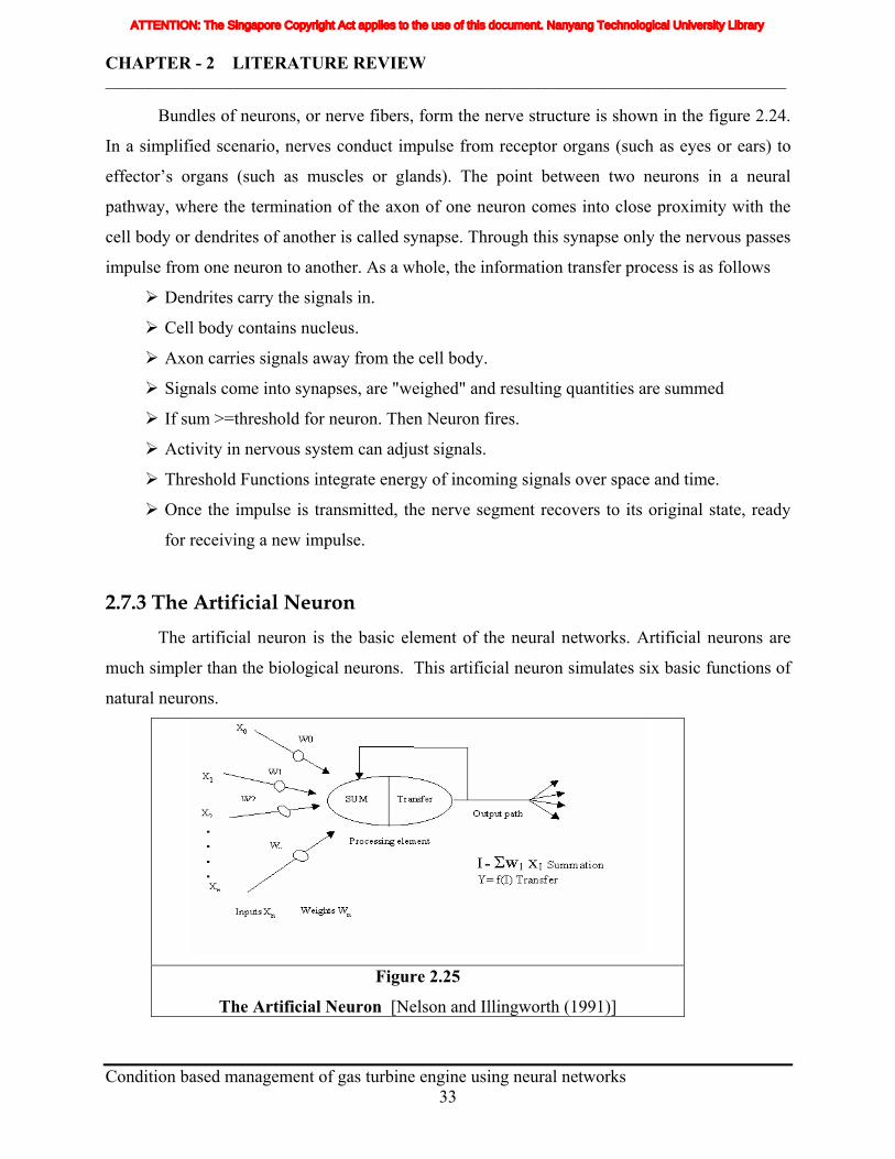
CHAPTER - 2 LITERATURE REVIEW _____________________________________________________________________________________________
Bundles of neurons, or nerve fibers, form the nerve structure is shown in the figure 2.24.
In a simplified scenario, nerves conduct impulse from receptor organs (such as eyes or ears) to
effector’s organs (such as muscles or glands). The point between two neurons in a neural
pathway, where the termination of the axon of one neuron comes into close proximity with the
cell body or dendrites of another is called synapse. Through this synapse only the nervous passes
impulse from one neuron to another. As a whole, the information transfer process is as follows
Dendrites carry the signals in.
Cell body contains nucleus.
Axon carries signals away from the cell body.
Signals come into synapses, are "weighed" and resulting quantities are summed
If sum >=threshold for neuron. Then Neuron fires.
Activity in nervous system can adjust signals.
Threshold Functions integrate energy of incoming signals over space and time.
Once the impulse is transmitted, the nerve segment recovers to its original state, ready
for receiving a new impulse.
2.7.3 The Artificial Neuron The artificial neuron is the basic element of the neural networks. Artificial neurons are
much simpler than the biological neurons. This artificial neuron simulates six basic functions of
natural neurons.
Figure 2.25
The Artificial Neuron [Nelson and Illingworth (1991)] Condition based management of gas turbine engine using neural networks
33
ATTENTION: The Singapore Copyright Act applies to the use of this document. Nanyang Technological University Library

CHAPTER - 2 LITERATURE REVIEW _____________________________________________________________________________________________
They are
behave
react
self-organize
learn
generalize
forget ……. Rather than executing the program.
Figure 2.25 shows the basics of artificial neuron. The various inputs to the network are
represented by the vectors such as X(1), X(2), X(3)…X(n). Each component of these inputs vectors
are multiplied by a corresponding vector components of connection weights, these weights are
represented by the vectors, such as W(1) W(2) W(3)…W(n). In the simplest case, the scalar result
obtained by the above multiplication are simply summed and passed through a transfer function
to generate an output. All artificial neural networks are constructed from this basic building
block with different structural arrangement depending on the need.
2.7.4.1 Neural Network Design
The neural network design is an iterative and complex process. It consists of the
following steps.
Arranging the neurons in various layers.
Deciding the type of connections among neurons for different layers as well as among the
neurons within a layer
Deciding the way a neuron receives input and produces output.
Determining the strength of connection within the network by allowing the network to
learn the appropriate values of connection weights using the training data sets.
The neural networks are the simple clustering of the artificial neurons. This clustering
occurs by creating layers, which are connected to each other. All the artificial neural networks
have a similar structure of topology.
The neurons are grouped into layers. The input layer consists of neurons that receive
input from the external environment. The output layer consists of neurons that communicate the
output of the system to the user or external environment. Figure 2.26 shows simple neural
network structure with one hidden layer, usually there will be larger number of hidden layer. Condition based management of gas turbine engine using neural networks
34
ATTENTION: The Singapore Copyright Act applies to the use of this document. Nanyang Technological University Library
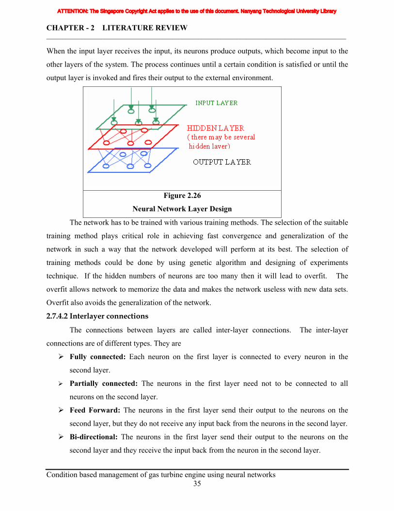
CHAPTER - 2 LITERATURE REVIEW _____________________________________________________________________________________________
When the input layer receives the input, its neurons produce outputs, which become input to the
other layers of the system. The process continues until a certain condition is satisfied or until the
output layer is invoked and fires their output to the external environment.
Figure 2.26
Neural Network Layer Design
The network has to be trained with various training methods. The selection of the suitable
training method plays critical role in achieving fast convergence and generalization of the
network in such a way that the network developed will perform at its best. The selection of
training methods could be done by using genetic algorithm and designing of experiments
technique. If the hidden numbers of neurons are too many then it will lead to overfit. The
overfit allows network to memorize the data and makes the network useless with new data sets.
Overfit also avoids the generalization of the network.
2.7.4.2 Interlayer connections
The connections between layers are called inter-layer connections. The inter-layer
connections are of different types. They are
Fully connected: Each neuron on the first layer is connected to every neuron in the
second layer.
Partially connected: The neurons in the first layer need not to be connected to all
neurons on the second layer.
Feed Forward: The neurons in the first layer send their output to the neurons on the
second layer, but they do not receive any input back from the neurons in the second layer.
Bi-directional: The neurons in the first layer send their output to the neurons on the
second layer and they receive the input back from the neuron in the second layer.
Condition based management of gas turbine engine using neural networks
35
ATTENTION: The Singapore Copyright Act applies to the use of this document. Nanyang Technological University Library
CHAPTER - 2 LITERATURE REVIEW _____________________________________________________________________________________________
Feed forward and bi-directional connections could be fully or partially connected.
Hierarchical: The neurons of a lower layer communicate with neurons on the next level
of layers.
Resonance: The layers have bi-directional connections and they continue to send
messages across the connections number of times, until a certain condition is achieved.
2.7.4.3 Intra-Layer connections
In more complex structures the neurons communicate among themselves within a layer,
this is known as intra-layer connections. There are two types of intra-layer connections.
Recurrent: The neurons within a layer are fully or partially connected to one another.
The neurons also receives input from another layer, they communicate their outputs with
one another before they are allowed to send their outputs to another layer.
On-centre/Off surround: A neuron within a layer has excitatory connections to itself,
with its immediate neighbors and has inhibitory connections to other neurons.
2.7.5.4 Learning
The brain basically learns from experience. Neural networks are sometimes called
machine learning algorithms, because changing of its connection weights (training) causes the
network to learn the solution to a problem. The strength of connection between the neurons is
stored as a weight value for the specific connection. The system learns new knowledge by
adjusting these connection weights. The learning ability of a neural network is determined by its
architecture and by the algorithmic method chosen for training. The training method usually
consists of one of three schemes.
Unsupervised learning: The hidden neurons must find a way to organize themselves
without the help from outside. In this approach, no sample outputs are provided to the
network against which it can measure its predictive performance for a given vector of
inputs.
Supervised learning: This method works on reinforcement from outside. The
connections among the neurons in the hidden layer are randomly arranged, then they
reshuffled in such a way that the network will be at its best performance level. Both
unsupervised learning and supervised learning suffer from relative slowness and
Condition based management of gas turbine engine using neural networks
36
ATTENTION: The Singapore Copyright Act applies to the use of this document. Nanyang Technological University Library
CHAPTER - 2 LITERATURE REVIEW _____________________________________________________________________________________________
inefficiency due to their dependence on the random shuffling to find the proper
connections of weights.
Back propagation: This method is proved highly successful in training the multilayered
neural nets. The network is not just given reinforcement for how it is doing on a task.
Information about errors is also filtered back through the system and is used to adjust the
connection between the layers and improves the performance of the network. It is a form
of supervised learning.
2.7.4.5 Learning Laws
There are varieties of learning laws in common use. These laws are mathematical
algorithms used to update the connection weights. The well-known Hebb's rule is main basis for
most of these laws.
Hebb's Rule: If a neuron receives an input from another neuron and if both are highly
active (mathematically have the same sign), the weight between the neuron should be
strengthened.
Hopfield Law: This law is similar to Hebb's Rule with the exception that it specifies the
magnitude of the strengthening or weakening. It states "if the desired output and the
input are both active or both inactive, increment the connection weight by the learning
rate otherwise decrement the weight by the learning rate respectively."
The Delta Rule: This rule changes the connection weights in such a way that leads to
minimizes the mean squared error of the network. The error is back propagated into
previous layer. The process of back-propagating the network errors continues until the
first layer is reached. It is also referred to as the Windrow-Hoff learning rule and the
Least mean square learning rule.
Kohonen's Learning Law: In the Kohonen's rule, the neurons compete for the
opportunity to learn or to update their weights. The processing neuron with the largest
output is declared the winner and has the capability of inhibiting its competitors as well
as exciting its neighbors. Only the winner is permitted to output and the winner plus its
neighbors are allowed to update their connection weights. This rule does not require
desired output. Therefore it is widely used in the unsupervised methods of learning.
Condition based management of gas turbine engine using neural networks
37
ATTENTION: The Singapore Copyright Act applies to the use of this document. Nanyang Technological University Library

CHAPTER - 2 LITERATURE REVIEW _____________________________________________________________________________________________
2.7.4.6 Application of Neural Networks
Neural networks are used in the areas ranging from robotics, speech, signal processing,
vision, and detection of heart malfunction etc. Basically most applications of neural networks fall
into the following five categories.
They are
Prediction: Uses input values to predict some output. e.g. pick the best stocks in the
market, predict weather, identify the people with cancer risk.
Classification: Use the input values to determine the classification. e.g. postal card
segregation based on the address.
Data association: It is similar to classification, but it also recognizes the data that
contains errors. e.g. not only identify the character that is scanned but also identify the
time when the scanner is not working properly.
Data conceptualization: Analyze the inputs so that grouping relationships can be
inferred. e.g. extract the names of a particular product from a database.
Data filtering: Smooth an input signal. e.g. removing the noise out of the telephone
signal.
2.7.5 Overview of Neural Network Structure The connectivity of a neural network determines its structure. It is broadly classified as
recurrent and non recurrent structures. Groups of neurons can be locally interconnected to form
“cluster” that are only loosely or indirectly connected to other clusters. Alternatively, neurons
can be organized into groups or layers that are connected (directionally) to other layers.
Following are the different types of neural network structures. [Schalkoff (1997)]
a. Feed Forward Neural Networks(FFNN)
b. Recurrent Neural Networks(RNN)
c. Competitive and Self-organizing Networks
d. Radial Basis Function Neural Networks (RBFNN)
e. Time Delay Neural Networks(TDNN) and
f. Fuzzy Neural Networks.
Condition based management of gas turbine engine using neural networks
38
ATTENTION: The Singapore Copyright Act applies to the use of this document. Nanyang Technological University Library
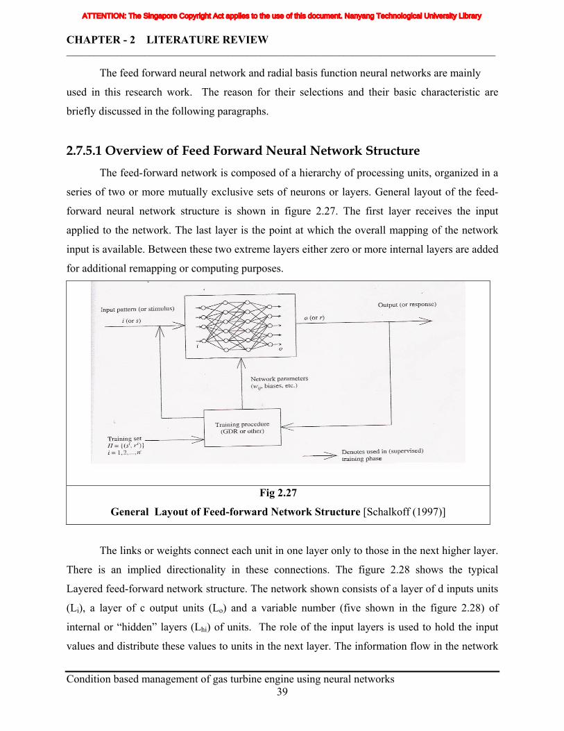
CHAPTER - 2 LITERATURE REVIEW _____________________________________________________________________________________________
The feed forward neural network and radial basis function neural networks are mainly
used in this research work. The reason for their selections and their basic characteristic are
briefly discussed in the following paragraphs.
2.7.5.1 Overview of Feed Forward Neural Network Structure The feed-forward network is composed of a hierarchy of processing units, organized in a
series of two or more mutually exclusive sets of neurons or layers. General layout of the feed-
forward neural network structure is shown in figure 2.27. The first layer receives the input
applied to the network. The last layer is the point at which the overall mapping of the network
input is available. Between these two extreme layers either zero or more internal layers are added
for additional remapping or computing purposes.
Fig 2.27
General Layout of Feed-forward Network Structure [Schalkoff (1997)]
The links or weights connect each unit in one layer only to those in the next higher layer.
There is an implied directionality in these connections. The figure 2.28 shows the typical
Layered feed-forward network structure. The network shown consists of a layer of d inputs units
(Li), a layer of c output units (Lo) and a variable number (five shown in the figure 2.28) of
internal or “hidden” layers (Lhi) of units. The role of the input layers is used to hold the input
values and distribute these values to units in the next layer. The information flow in the network
Condition based management of gas turbine engine using neural networks
39
ATTENTION: The Singapore Copyright Act applies to the use of this document. Nanyang Technological University Library
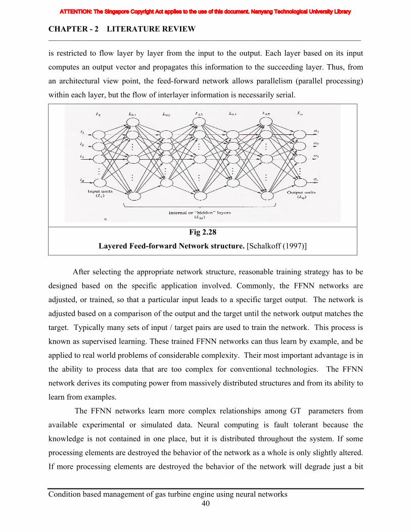
CHAPTER - 2 LITERATURE REVIEW _____________________________________________________________________________________________
is restricted to flow layer by layer from the input to the output. Each layer based on its input
computes an output vector and propagates this information to the succeeding layer. Thus, from
an architectural view point, the feed-forward network allows parallelism (parallel processing)
within each layer, but the flow of interlayer information is necessarily serial.
Fig 2.28
Layered Feed-forward Network structure. [Schalkoff (1997)]
After selecting the appropriate network structure, reasonable training strategy has to be
designed based on the specific application involved. Commonly, the FFNN networks are
adjusted, or trained, so that a particular input leads to a specific target output. The network is
adjusted based on a comparison of the output and the target until the network output matches the
target. Typically many sets of input / target pairs are used to train the network. This process is
known as supervised learning. These trained FFNN networks can thus learn by example, and be
applied to real world problems of considerable complexity. Their most important advantage is in
the ability to process data that are too complex for conventional technologies. The FFNN
network derives its computing power from massively distributed structures and from its ability to
learn from examples.
The FFNN networks learn more complex relationships among GT parameters from
available experimental or simulated data. Neural computing is fault tolerant because the
knowledge is not contained in one place, but it is distributed throughout the system. If some
processing elements are destroyed the behavior of the network as a whole is only slightly altered.
If more processing elements are destroyed the behavior of the network will degrade just a bit
Condition based management of gas turbine engine using neural networks
40
ATTENTION: The Singapore Copyright Act applies to the use of this document. Nanyang Technological University Library
CHAPTER - 2 LITERATURE REVIEW _____________________________________________________________________________________________
further, whereas traditional computing systems are rendered useless by even small amounts of
damage to the memory.
The FFNN is considered as universal approximators due to its capability of approximating
any finite function to any degree of accuracy. But still there are many practical unresolved
issues, especially those related to the effects of training or learning. However it is concluded as
follows [J.Scchalkoff (1997)].
FF ANN networks with a single hidden layer are capable of approximating the class of
“useful” functions.
Lack of success in applications must be attributable due to
a. Faulty training.
b. Faulty architecture (eg. Incorrect numbers of hidden units)
c. Lack of a functional relationship between input and output.
The mapping power of the FF ANN is not inherent of the choice of specific activation
function rather it is the multilayer feed-forward structure that leads to the general function
approximation capability.
In general, the learning rule applied to the feed-forward neural network is mainly
classified into two types
a. Error adjusting and
b. Gradient adjusting rule.
The error adjusting rule, adjust the connecting weights between nodes of adjacent layers
according to errors between the current output and their expected output. In the gradient
adjusting rule, the weights based on the gradient variation of the mean square errors between the
current output and their expected output of all training samples.
The adjusting weights for the error-adjusting rule is given in equation no.1
W t+1 = W + η. (Yt-Ot). Xi [1]
Where W is defined as weights, Xi is input vector; η is learning rate, Yt and Ot are the
expected output and current output respectively. Convergence speed of this rule is faster, but it
valid only for the single layer neural network.
δE (W) / δWji = ΣPp=1 Σ M
m=1(Ypk- Opk).Opk.(1-Opk) [ 2]
Condition based management of gas turbine engine using neural networks
41
The gradient of the mean square error to weight for the gradient adjusting rule has been
given in equation no.2; Where P is number of training samples. M is number of nodes in output
ATTENTION: The Singapore Copyright Act applies to the use of this document. Nanyang Technological University Library
CHAPTER - 2 LITERATURE REVIEW _____________________________________________________________________________________________
layer. Ypk is the expected output of sample p. Opk is the current output of the sample p. E is the
mean square error. Wji is the weight connecting layer i and j.
It is obvious that the weights adjusting equation includes three factors, (Ypk- Opk), Opk
and (1-Opk). It can be concluded that when the gradient tends to zero; we can not simply infer
that the iteration has completed and reached required accuracy of iteration. The cases may exist
that Opk or (1-Opk) tends to zero while (Ypk-Opk) is still very large. In this case, the training
process has fallen into static area where convergence speed becomes very slow. Many
improvements have been made in traditional BP algorithm to solve this problem, such as variable
iteration step length, conjugate gradient and the least square algorithm. Although these
improvements have some positive effects, the expediting convergence speed is at the cost of
complexity of iteration and net structure.
The Feed-forward Back-Propagation Network (FFBPN) has been chosen for forecasting
the various gas turbine healths indicating parameters (GHI) are due to the following reasons
a. Its ability to approximate any finite function to high accuracy level.
b. The BPN has got high ability to recognize the fault patterns despite the presence of noise.
(Some fault data would not totally destroy the network performance).
c. Its flexibility and straightforward structure makes it more suitable.
d. Success achieved by many researchers like Lorenzo et al (2002) & Neophytos et al(2002)
in the application of feed-forward neural networks for modeling the complex gas turbine
health indicating parameters has also favored the use of this BPN for forecasting various
health indicating parameters of this research work.
2.7.5.2 Overview of Radial Basis Function Neural Networks (RBFNNs)
In the nervous system of biological organisms there is evidence of neurons whose
response characteristics are “local” or “tuned” to some region of input space. Best example is the
orientation of sensitive cells of the visual cortex, whose response is sensitive to local regions of
the retina.
The RBF network is a feed-forward structure with a modified hidden layer and training
algorithm used for mapping. It consists of the input layer, a radial basis layer and the competitive
layer. When an input is presented, the radial basis layer computes distances from the input
vector to the training input vectors, and produces a vector whose elements indicate how close the Condition based management of gas turbine engine using neural networks
42
ATTENTION: The Singapore Copyright Act applies to the use of this document. Nanyang Technological University Library
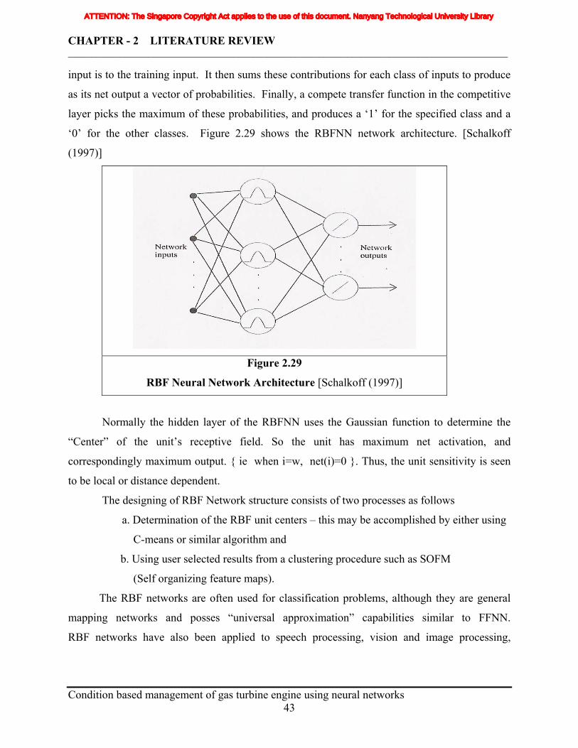
CHAPTER - 2 LITERATURE REVIEW _____________________________________________________________________________________________
input is to the training input. It then sums these contributions for each class of inputs to produce
as its net output a vector of probabilities. Finally, a compete transfer function in the competitive
layer picks the maximum of these probabilities, and produces a ‘1’ for the specified class and a
‘0’ for the other classes. Figure 2.29 shows the RBFNN network architecture. [Schalkoff
(1997)]
Figure 2.29
RBF Neural Network Architecture [Schalkoff (1997)]
Normally the hidden layer of the RBFNN uses the Gaussian function to determine the
“Center” of the unit’s receptive field. So the unit has maximum net activation, and
correspondingly maximum output. { ie when i=w, net(i)=0 }. Thus, the unit sensitivity is seen
to be local or distance dependent.
The designing of RBF Network structure consists of two processes as follows
a. Determination of the RBF unit centers – this may be accomplished by either using
C-means or similar algorithm and
b. Using user selected results from a clustering procedure such as SOFM
(Self organizing feature maps).
The RBF networks are often used for classification problems, although they are general
mapping networks and posses “universal approximation” capabilities similar to FFNN.
RBF networks have also been applied to speech processing, vision and image processing,
Condition based management of gas turbine engine using neural networks
43
ATTENTION: The Singapore Copyright Act applies to the use of this document. Nanyang Technological University Library
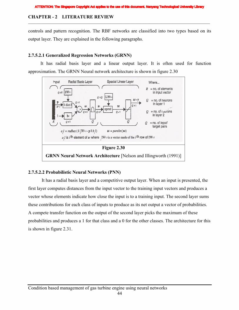
CHAPTER - 2 LITERATURE REVIEW _____________________________________________________________________________________________
controls and pattern recognition. The RBF networks are classified into two types based on its
output layer. They are explained in the following paragraphs.
2.7.5.2.1 Generalized Regression Networks (GRNN)
It has radial basis layer and a linear output layer. It is often used for function
approximation. The GRNN Neural network architecture is shown in figure 2.30
Figure 2.30
GRNN Neural Network Architecture [Nelson and Illingworth (1991)]
2.7.5.2.2 Probabilistic Neural Networks (PNN)
It has a radial basis layer and a competitive output layer. When an input is presented, the
first layer computes distances from the input vector to the training input vectors and produces a
vector whose elements indicate how close the input is to a training input. The second layer sums
these contributions for each class of inputs to produce as its net output a vector of probabilities.
A compete transfer function on the output of the second layer picks the maximum of these
probabilities and produces a 1 for that class and a 0 for the other classes. The architecture for this
is shown in figure 2.31.
Condition based management of gas turbine engine using neural networks
44
ATTENTION: The Singapore Copyright Act applies to the use of this document. Nanyang Technological University Library
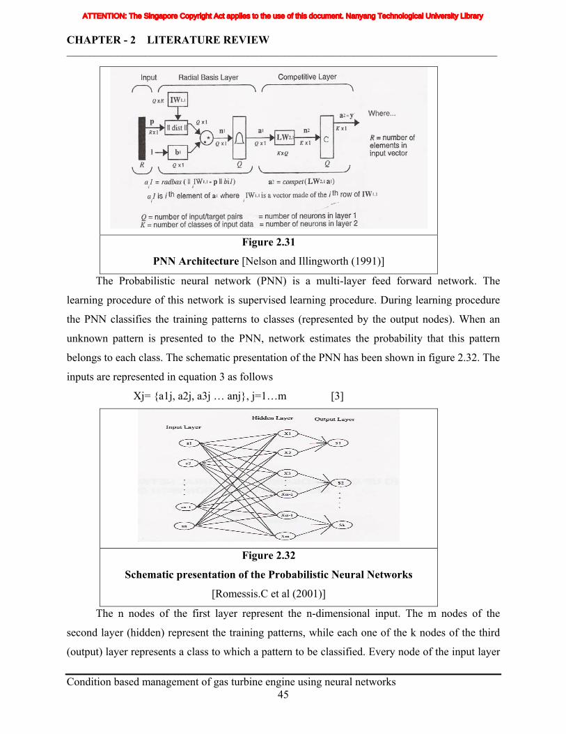
CHAPTER - 2 LITERATURE REVIEW _____________________________________________________________________________________________
Figure 2.31
PNN Architecture [Nelson and Illingworth (1991)]
The Probabilistic neural network (PNN) is a multi-layer feed forward network. The
learning procedure of this network is supervised learning procedure. During learning procedure
the PNN classifies the training patterns to classes (represented by the output nodes). When an
unknown pattern is presented to the PNN, network estimates the probability that this pattern
belongs to each class. The schematic presentation of the PNN has been shown in figure 2.32. The
inputs are represented in equation 3 as follows
Xj= {a1j, a2j, a3j … anj}, j=1…m [3]
Figure 2.32
Schematic presentation of the Probabilistic Neural Networks
[Romessis.C et al (2001)]
The n nodes of the first layer represent the n-dimensional input. The m nodes of the
second layer (hidden) represent the training patterns, while each one of the k nodes of the third
(output) layer represents a class to which a pattern to be classified. Every node of the input layer Condition based management of gas turbine engine using neural networks
45
ATTENTION: The Singapore Copyright Act applies to the use of this document. Nanyang Technological University Library
CHAPTER - 2 LITERATURE REVIEW _____________________________________________________________________________________________
of the PNN is linked to every node of the hidden layer. Each node of the hidden layer
(representing a training pattern) is linked only to the node of the output layer that represents the
class where the training pattern ‘belongs’. When a pattern x Є Rm is given as an input to the
network, the output is the probability density functions: P(Si|x), i= 1, 2, ..k. If we assume that the
probability density functions, P (x|Si) are Gaussian, It is represent in equation 4 as follows
P (Si|x) = [P (Si) / P(x).(2П)m/2.σim . |Si|] . Σ ni j=1 exp [-(x-xj
(i))T(x-xj(i)) / 2σi
2] [4].
Where, xj(i) is the j-th pattern of the training set of patterns that belong to class i, |Si|=ni is
the number of the training patterns that to class i, σi is a smoothing parameter, P(Si) is the ‘a
priori’ probability of class Si, and P(x) a normalization factor representing the ‘a priori’
probability of pattern x, which is constant assuming mutually exclusive classes, covering all
possible situations. If we assume ‘a priori’ probability is equal for all classes.
Then P(Si)= 1/k, {I = 1,2,…,k}
Selection of the PNN network for the comparison of actual gas turbine health indicating
parameter with the guaranteed and expected values provided by the manufacture is due to the
following reason
a. The PNN networks are more useful for classification problems.
b. Their design is straight forward and guaranteed to converge to a Bayesian classifier
provided it is given enough training data.
c. These networks generalize well.
d. Better suitability of probability density functions to analyze the degradation rate of the gas
turbine. It is explained in the following paragraphs.
Probabilistic based techniques utilizes the known information on how the gas turbine
health indicating parameters degrade over time to assess the current severity of the parameter
distributions shifts and project their future state. This prognostic modeling approach concept has
been shown in the figure 2.33. The parameter space is populated by two main components. These
are the current condition and expected degradation path. Both are multi-variate Probability
density function (PDFs) or 3-D statistical distributions. [Gregory et al (2001).]
Condition based management of gas turbine engine using neural networks
46
ATTENTION: The Singapore Copyright Act applies to the use of this document. Nanyang Technological University Library
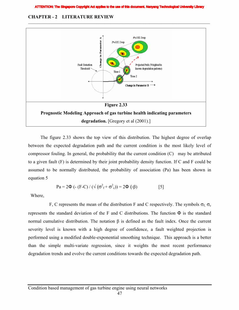
CHAPTER - 2 LITERATURE REVIEW _____________________________________________________________________________________________
Figure 2.33
Prognostic Modeling Approach of gas turbine health indicating parameters
degradation. [Gregory et al (2001).]
The figure 2.33 shows the top view of this distribution. The highest degree of overlap
between the expected degradation path and the current condition is the most likely level of
compressor fouling. In general, the probability that the current condition (C) may be attributed
to a given fault (F) is determined by their joint probability density function. If C and F could be
assumed to be normally distributed, the probability of association (Pa) has been shown in
equation 5
Pa = 2Φ (- (F-C) / (√ (σ2f + σ2
c)) = 2Φ (-β) [5]
Where,
F, C represents the mean of the distribution F and C respectively. The symbols σf, σc
represents the standard deviation of the F and C distributions. The function Φ is the standard
normal cumulative distribution. The notation β is defined as the fault index. Once the current
severity level is known with a high degree of confidence, a fault weighted projection is
performed using a modified double-exponential smoothing technique. This approach is a better
than the simple multi-variate regression, since it weights the most recent performance
degradation trends and evolve the current conditions towards the expected degradation path.
Condition based management of gas turbine engine using neural networks
47
ATTENTION: The Singapore Copyright Act applies to the use of this document. Nanyang Technological University Library
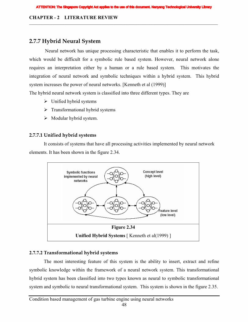
CHAPTER - 2 LITERATURE REVIEW _____________________________________________________________________________________________
2.7.7 Hybrid Neural System Neural network has unique processing characteristic that enables it to perform the task,
which would be difficult for a symbolic rule based system. However, neural network alone
requires an interpretation either by a human or a rule based system. This motivates the
integration of neural network and symbolic techniques within a hybrid system. This hybrid
system increases the power of neural networks. [Kenneth et al (1999)]
The hybrid neural network system is classified into three different types. They are
Unified hybrid systems
Transformational hybrid systems
Modular hybrid system.
2.7.7.1 Unified hybrid systems
It consists of systems that have all processing activities implemented by neural network
elements. It has been shown in the figure 2.34.
Figure 2.34
Unified Hybrid Systems [ Kenneth et al(1999) ]
2.7.7.2 Transformational hybrid systems
The most interesting feature of this system is the ability to insert, extract and refine
symbolic knowledge within the framework of a neural network system. This transformational
hybrid system has been classified into two types known as neural to symbolic transformational
system and symbolic to neural transformational system. This system is shown in the figure 2.35. Condition based management of gas turbine engine using neural networks
48
ATTENTION: The Singapore Copyright Act applies to the use of this document. Nanyang Technological University Library
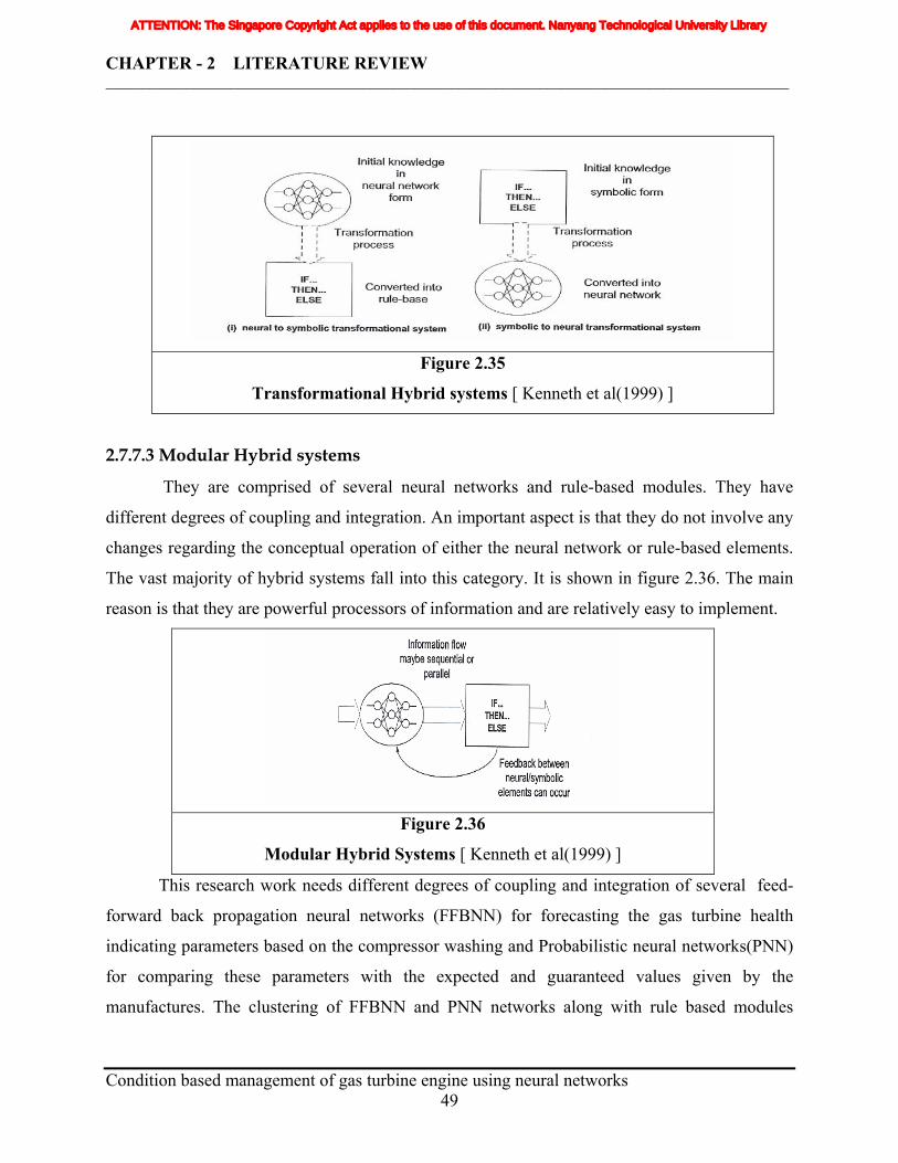
CHAPTER - 2 LITERATURE REVIEW _____________________________________________________________________________________________
Figure 2.35
Transformational Hybrid systems [ Kenneth et al(1999) ]
2.7.7.3 Modular Hybrid systems
They are comprised of several neural networks and rule-based modules. They have
different degrees of coupling and integration. An important aspect is that they do not involve any
changes regarding the conceptual operation of either the neural network or rule-based elements.
The vast majority of hybrid systems fall into this category. It is shown in figure 2.36. The main
reason is that they are powerful processors of information and are relatively easy to implement.
Figure 2.36
Modular Hybrid Systems [ Kenneth et al(1999) ]
This research work needs different degrees of coupling and integration of several feed-
forward back propagation neural networks (FFBNN) for forecasting the gas turbine health
indicating parameters based on the compressor washing and Probabilistic neural networks(PNN)
for comparing these parameters with the expected and guaranteed values given by the
manufactures. The clustering of FFBNN and PNN networks along with rule based modules
Condition based management of gas turbine engine using neural networks
49
ATTENTION: The Singapore Copyright Act applies to the use of this document. Nanyang Technological University Library

CHAPTER - 2 LITERATURE REVIEW _____________________________________________________________________________________________
without any changes in the conceptual operation systems shows the requirement of the modular
hybrid system for this research work.
2.8 Introduction to develop the neural network model using
Matlab toolbox
2.8.1. Creation of Feed Forward network using Matlab toolbox 2.8.1.1 Network creation
The function newff creates a feedforward network. It requires four inputs and returns the
network object. The first input is an R by 2 matrix of minimum and maximum values for each of
the R elements of the input vector. The second input is an array containing the sizes of each
layer. The third input is a cell array containing the names of the transfer functions to be used in
each layer. The final input contains the name of the training function to be used.
For example, the following command creates a two-layer feedforward network. There is
one input vector with two elements.
e.g. net = newff([-1 2; 0 5],[3,1],{'tansig', 'purelin'}, 'traingd');
The values for the first element of the input vector range between –1 and 2, the values of
the second element of the input vector range between 0 and 5. There are three neurons in the first
layer and one neuron in the second (output) layer. The transfer function in the first layer is tan-
sigmoid and the output layer transfer function is pure linear. The training function used is
traingd. The above command creates the network object, also initializes the weights and biases of
the network.
2.8.1.2 Training the network
The network is ready for training after initializing the weights and biases. The training
process requires a set of examples with network inputs p and target outputs t. During training the
weights and biases of the network are iteratively adjusted to minimize the network performance.
For the feed forward network the default performance function is mean square error. (MSE).
The following code is used to train the network.
[net, tr ]=train (net, p, t);
The training record tr contains information about the progress of training.
Condition based management of gas turbine engine using neural networks
50
ATTENTION: The Singapore Copyright Act applies to the use of this document. Nanyang Technological University Library
CHAPTER - 2 LITERATURE REVIEW _____________________________________________________________________________________________
Different algorithms are available for training the feed forward network. They use the
gradient of the performance function to determine the weights to minimize performance (MSE).
In the basic back-propagation algorithm, the weights are moved in the direction of the negative
gradient. There are various types of training algorithms are available. They are
Batch training (train), batch gradient descent (traingd), batch gradient descent with
momentum algorithm (traingdm), variable learning rate algorithms (traingda, traingdx), resilent
backpropagation algorithm (trainrp), conjugate gradient algorithms (traincgf, traincgp, traincgb,
trainscg) and line search routine algorithms (srchgol, srchbre, srchhyb, srchcha, srchbac), Quasi-
Newton algorithms(trainbgf, trainoss) and Levenberg-Marquardt algorithm (trainlm).
2.8.1.3 Simulation of the network
The function sim simulates a network. sim command takes the network input p, and the
network object net, and returns the network outputs a. The following command is used to
simulate the network.
a = sim(net,p)
Where a is the output, net is network and p is the input.
2.8.1.4 Preprocessing and postprocessing techniques
Neural network training would be made more efficient if certain preprocessing steps have
been performed on the network inputs and targets. This section describes various preprocessing
routines.
2.8.1.4.1 Min and Max (premnmax, postmnmx,tramnmx)
The function premnmx are used to scale the inputs and targets so that they fall in the
range of –1 to 1. The following codes illustrates the use of this function
[pn, minp, maxp,tn,mint, maxt] = premnmx(p,t);
net = train(net, pn, tn);
The original network inputs and targets are given in the matrix p and t respectively. The
normalized inputs and targets are pn and tn respectively. The values of pn and tn would be in the
range of –1 to 1. The vectors minp and maxp contain the minimum and maximum values of the
original inputs, and the vectors mint and maxt contains the minimum and maximum values of the Condition based management of gas turbine engine using neural networks
51
ATTENTION: The Singapore Copyright Act applies to the use of this document. Nanyang Technological University Library
CHAPTER - 2 LITERATURE REVIEW _____________________________________________________________________________________________
original targets. The following codes will simulate the network that is trained by using previous
codes, and normalize back the network output into the original units.
an = sim(net,pn);
a = postmnmx(an, mint, maxt);
Whenever the trained network is used with new inputs they have to be preprocessed with
the minimum and maximums computed for the training set. This is accomplished with the
routine tramnmx. The following set of codes are used to simulate the new set of inputs to the
network, which have been trained previously.
pnewn = tramnmx(pnew, minp, maxp);
anewn = sim(net, pnewn);
anew = postmnmx( anewn, mint, maxt);
2.8.1.4.2 Mean and Standard deviation ( prestd, postd, trastd)
This method normalizes the inputs and targets so that they will have zero mean and unity
standard deviation. The following code illustrates the use of prestd.
[pn,meanp,stdp,tn,meant,stdt]=prestd(p,t);
net = train (net, pn, tn);
The original network inputs and targets are given in the matrices p and t. The pn and tn
are the normalized inputs and targets respectively, they will have zero means and unity standard
deviation. The vectors meanp and stdp contains the mean and standard deviations of the original
inputs. The vectors meant and stdt contains the mean and the standard deviations of the original
targets. The following codes are used to simulate the previously trained network and then
convert the network output back into the original units.
an = sim(net,pn)
a = poststd( an, meant, stdt);
Whenever the trained network is used with new inputs they have to be preprocessed with
the means and standard deviations that were computed for the training set. This is accomplished
with the routine trastd. The following set of codes are used to simulate the new set of inputs to
the network which we have been trained previously.
Condition based management of gas turbine engine using neural networks
52
ATTENTION: The Singapore Copyright Act applies to the use of this document. Nanyang Technological University Library
CHAPTER - 2 LITERATURE REVIEW _____________________________________________________________________________________________
pnewn =trastd(pnew,meanp,stdp);
anewn=sim(net,pnewn);
anew =poststd(anew,meant,stdt);
2.8.2 Creation of Probabilistic Neural network model using Matlab
toolbox Probabilistic neural network (PNN) is used for the classification problems. Their design
is straightforward and does not solely depend on training. This network generalizes well. The
procedure for design a PNN in Matlab toolbox is briefly discussed as follows,
The inputs and targets have to be presented in the form of matrix.
e.g four input vectors and their corresponding targets are presented into the network as follows
P = [0 0; 1 1; 0 3; 1 4] ; Tc = [ 1 2 3 4 ];
The target matrix is to be provided with 1's at the right places. The function ind2vec is used to
create a matrix with 0's except at the correct spots. The following code illustrates the creation of
the required target matrix.
T = ind2vec(Tc)
The new matrix T is in the following format
T =
(1,1) 1
(2,2) 1
(3,3) 1
(4,4) 1
The function newpnn is used to create the PNN network.
net=newpnn(P,T);
sim function is used to simulate the developed network.
Y=sim(net,P);
Condition based management of gas turbine engine using neural networks
53
ATTENTION: The Singapore Copyright Act applies to the use of this document. Nanyang Technological University Library

CHAPTER - 2 LITERATURE REVIEW _____________________________________________________________________________________________
Condition based management of gas turbine engine using neural networks
54
The following code has to be used to convert the output Y into a row Yc to make the
classifications clear.
Yc =vec2ind(Y);
Final output is in the following format.
Yc = 1 2 3 4
ATTENTION: The Singapore Copyright Act applies to the use of this document. Nanyang Technological University Library
CHAPTER 3 – MODEL DEVELOPMENT _____________________________________________________________________________________________
3.1 Gas turbine degradation models development Thermodynamic degradation models for V94.3A gas turbine have been developed using
matlab programming language and then these thermodynamic models are used to train the neural
network model. These models need gas turbine operating parameters for more than 8000 EOH
(>11 months) to learn the behavior of recoverable and non-recoverable losses of the gas turbine
compressor. After training, the neural network model is used to segregate the recoverable & non-
recoverable losses of the gas turbine compressor and suggest the suitable washing plan to
minimize them after including the cost effects. These models serve as a good tool for the
reducing the long term performance degradation of gas turbine due to its compressor fouling.
3.1.1 Measured parameters available on site
The measured parameters available on the site play a crucial role in selecting a method
for calculating various gas turbine health indicating (GHI) parameters. [Bhargava Rakesh
(1992)]. Figure 3.1 shows the measured parameters available under the site conditions. These
parameters are continuously monitored by the operating systems available in the control room
and they are available in both on-line and off-line formats.
3.2 Development of thermodynamic models to assess the gas turbine
compressor performance The following parameters play very crucial role in determining the gas turbine
compressor performance.
Compressor polytropic efficiency.
Compressor isentropic efficiency.
Pressure ratio.
Power output of CCPP.
Thermal Efficiency of CCPP.
Heat rate of CCPP and
Compressor air flow rate.
Condition based management of gas turbine engine using neural networks 55
ATTENTION: The Singapore Copyright Act applies to the use of this document. Nanyang Technological University Library
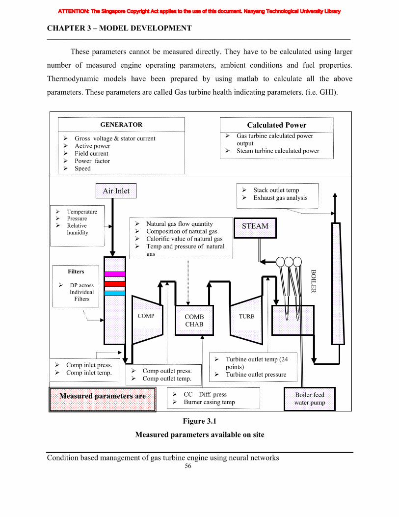
CHAPTER 3 – MODEL DEVELOPMENT _____________________________________________________________________________________________
These parameters cannot be measured directly. They have to be calculated using larger
number of measured engine operating parameters, ambient conditions and fuel properties.
Thermodynamic models have been prepared by using matlab to calculate all the above
parameters. These parameters are called Gas turbine health indicating parameters. (i.e. GHI).
Calculated Power Gas turbine calculated power
output Steam turbine calculated power
GENERATOR
Gross voltage & stator current Active power Field current Power factor Speed
BO
ILER
STEAM
Boiler feed water pump
Turbine outlet temp (24 points)
Turbine outlet pressure
TURB
Natural gas flow quantity Composition of natural gas. Calorific value of natural gas Temp and pressure of natural
gas
CC – Diff. press Burner casing temp
COMB CHAB
Comp outlet press. Comp outlet temp.
COMP
Comp inlet press. Comp inlet temp.
Filters
DP across Individual
Filters
Temperature Pressure Relative
humidity
Air Inlet Stack outlet temp Exhaust gas analysis
Co
ATTENTION: The Singapore Copyright Act applies to the use of this document. Nanyang Technological University Library
in dotted boxes Measured parameters are
Figure 3.1
Measured parameters available on site
ndition based management of gas turbine engine using neural networks 56
CHAPTER 3 – MODEL DEVELOPMENT _____________________________________________________________________________________________
3.2.1 Polytropic, Isentropic & Pressure ratio Calculation The polytropic, isentropic and pressure ratio of the gas turbine compressor are
determined by using compressor's inlet, outlet temperatures and pressures. These health-
monitoring parameters give clear indication about the cleanliness of the compressor blades.
Refer to appendix A2 for details about the procedure used for calculating these health-indicating
parameters. [IGTI (1995)].
3.2.2 Generator efficiency & coupling gross power output calculation The generator efficiency and coupling gross output are calculated using the measured
gross power output, gross generator voltage, gross current, field current, power factor. See the
appendix A3 for details about the calculation procedure used. The calculated efficiency, coupling
gross power output and net power outputs have been corrected to the generator design power
factor of 0.85. This correction helps to do the comparison of gross coupling power output and
generator efficiency under various operating conditions.
3.2.3 Determination of mass flow rate, calorific value & carbon hydrogen
ratio of fuel gas The mass flow rate, calorific value and carbon hydrogen ratio of fuel gas are the critical
parameters needed to determine the fuel gas power input to the gas turbine. The ISO 12213
standard has been used for determining fuel gas density. This calculation is very complicated, so
the free software package using AGA8-92DC method has been used to determine the density of
the fuel gas. The fuel gas composition (%mole), pressure and temperature of the fuel gas are
given as inputs to this software AGA8-92DC and it gives the density of the fuel gas composition.
The mass flow rate of the fuel gas is determined using the following formula
Fuel gas mass flow rate = Fuel gas volumetric flow rate x Density of fuel gas
composition.
The lower calorific value, higher calorific value and carbon hydrogen ratios of the fuel
gas composition are determined as per the procedure given in the appendix A4.
Condition based management of gas turbine engine using neural networks 57
ATTENTION: The Singapore Copyright Act applies to the use of this document. Nanyang Technological University Library
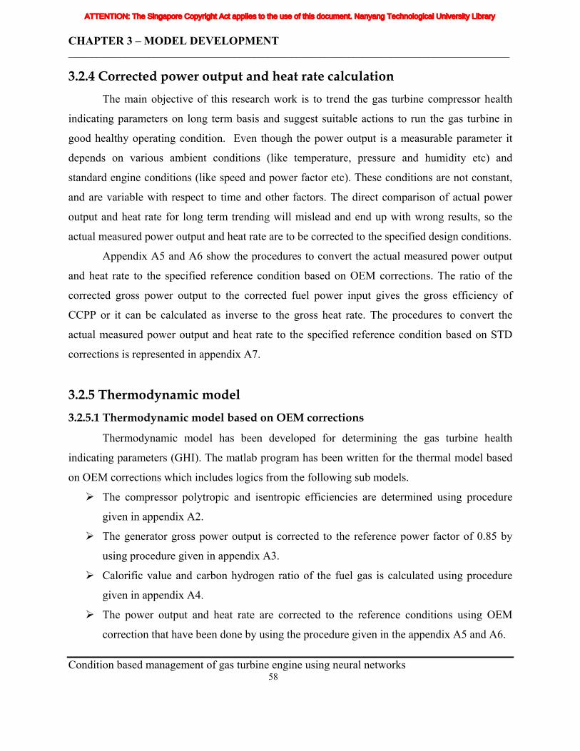
CHAPTER 3 – MODEL DEVELOPMENT _____________________________________________________________________________________________
3.2.4 Corrected power output and heat rate calculation The main objective of this research work is to trend the gas turbine compressor health
indicating parameters on long term basis and suggest suitable actions to run the gas turbine in
good healthy operating condition. Even though the power output is a measurable parameter it
depends on various ambient conditions (like temperature, pressure and humidity etc) and
standard engine conditions (like speed and power factor etc). These conditions are not constant,
and are variable with respect to time and other factors. The direct comparison of actual power
output and heat rate for long term trending will mislead and end up with wrong results, so the
actual measured power output and heat rate are to be corrected to the specified design conditions.
Appendix A5 and A6 show the procedures to convert the actual measured power output
and heat rate to the specified reference condition based on OEM corrections. The ratio of the
corrected gross power output to the corrected fuel power input gives the gross efficiency of
CCPP or it can be calculated as inverse to the gross heat rate. The procedures to convert the
actual measured power output and heat rate to the specified reference condition based on STD
corrections is represented in appendix A7.
3.2.5 Thermodynamic model 3.2.5.1 Thermodynamic model based on OEM corrections
Thermodynamic model has been developed for determining the gas turbine health
indicating parameters (GHI). The matlab program has been written for the thermal model based
on OEM corrections which includes logics from the following sub models.
The compressor polytropic and isentropic efficiencies are determined using procedure
given in appendix A2.
The generator gross power output is corrected to the reference power factor of 0.85 by
using procedure given in appendix A3.
Calorific value and carbon hydrogen ratio of the fuel gas is calculated using procedure
given in appendix A4.
The power output and heat rate are corrected to the reference conditions using OEM
correction that have been done by using the procedure given in the appendix A5 and A6. Condition based management of gas turbine engine using neural networks 58
ATTENTION: The Singapore Copyright Act applies to the use of this document. Nanyang Technological University Library
CHAPTER 3 – MODEL DEVELOPMENT _____________________________________________________________________________________________
The thermal model including all the above steps has been shown in the appendix A7.
SNo. INPUTS SNo. OUTPUTS 1 Compressor inlet temp 1 Corrected gross power output 2 Compressor outlet temp 2 Corrected heat rate 3 Compressor outlet press 3 Gross CCPP thermal efficiency 4 Ambient press 4 Compressor polytropic efficiency 5 Condensor water inlet temp 5 Compressor isentropic efficiency 6
Gen
eral
T
herm
al
Prop
ertie
s
Turbine speed 6 Compressor pressure ratio 7 Nitrogen content 7 Lower calorific value of fuel gas 8 Co2 content 8 Fuel input power 9 Methane content 9 Carbon hydrogen ratio of fuel gas
10 Ethane content 11 Propane content 12 I-Butane content 13 N-Butane content 14 I-Pentane content 15 N-Pentane content 16 N-Hexane content 17 N-Heptane content 18 N-0ctane content 19 N-Nonane content 20
Fue
l Gas
Pro
pert
ies
Fuel mass flow rate
22 Active power 10 Gross Power generator at coupling 23 Gen reactive power 11 Generator efficiency 24 Gross current 12 Gross power corrected to 0.85 pf 25 Power factor 26 Gross voltage 27
Gen
erat
or
Det
ails
Field current
Table 3.1
Inputs and Outputs for the thermodynamic model of the gas turbine engine
Appendix B1 contains details of the matlab program for the thermodynamic model based
on OEM corrections. Table 3.1 represents the input and output parameters to the
thermodynamic model. Table 3.2 in Appendix C1 represents the inputs and outputs for the
above thermodynamic model based on OEM corrections at various EOH.
Condition based management of gas turbine engine using neural networks 59
ATTENTION: The Singapore Copyright Act applies to the use of this document. Nanyang Technological University Library
CHAPTER 3 – MODEL DEVELOPMENT _____________________________________________________________________________________________
3.2.5.2 Thermodynamic model based on STD corrections
The matlab program has been written for the thermal model based on OEM corrections
which includes logics from the following sub models.
The power output and heat rate are corrected to the reference conditions using STD
corrections have been done by using the procedure given in appendix A8.
The remaining procedures are similar to the thermodynamic model based on OEM
corrections. Appendix A7 gives the details about the thermodynamic model.
The matlab programming has been written for the thermal model based on STD corrections.
Refer to appendix B2 for the details about the program. Table 3.1 represents the input and output
parameters to this thermodynamic model also. Table 3.3 in Appendix C2 represents the inputs
and outputs for the above thermodynamic model based on STD corrections at various EOH.
3.2.6 Air flow rate Calculation Most of the Industrial gas turbines used for power generation are of larger capacities, the
air flow rate through the compressor and turbine inlet temperature of gas turbines are not
measured directly due to very high amount of air flow (e.g.,> 620kg/s) into the compressor, very
high turbine inlet temperature (e.g., >1200˚C) and their higher variation inside the combustion
chamber. But these two parameters play critical role in determining the health condition of the
individual components of gas turbine and the efficiency of the engine. Various methods available
to determine the airflow rate are
a. Using compressor characteristic curve.
b. Stage stacking technique.
c. Differential pressure method.
d. Combustion analysis using exhaust dry oxygen.
e. Mass and energy balance method.
Condition based management of gas turbine engine using neural networks 60
ATTENTION: The Singapore Copyright Act applies to the use of this document. Nanyang Technological University Library
CHAPTER 3 – MODEL DEVELOPMENT _____________________________________________________________________________________________
3.2.6.1 Model compressor characteristic curve given by OEM
The model characteristic given by the manufacture is a 3D graph, which inter-relates the
airflow with respect to speed and pressure ratio of the compressor. It shows only the shape of the
curve and it does not consist of any numerical value. This curve cannot be used for determining
the accurate value of airflow, which is a must for this research work. Therefore this method is
eliminated.
3.2.6.2 Stage stacking method
Complicate compressor blade and rotor internal dimensional details are required for
using this method. Since it is very difficult to get all these details, application of this method is
also eliminated.
3.2.6.3 Differential pressure method:
In the differential pressure method a plot of the ratio of scroll differential pressure to
inlet static pressure (∆P /PIC) Vs referred speed (NRef) has to be created to find out how the
compressor air flow is getting varied with respect to time period.
∆P Measured inlet scroll differential pressure, in. H20
____ = __________________________________________
PIC Compressor inlet absolute static pressure, in H20
Referred speed, NRef = N / SQRT ((TIC)(R) / ( 540°R) (53.532 lbf-ft /lbm – °R))
The compressor inlet temperature (TIC), gas constant(R) and Speed (N) are used to find out the
referred speed (N Ref).
Concept of this method – In general the entrance to the compressor acts like a nozzle and
(∆P /PIC) is therefore an indicator of airflow. A gradual decrease in (∆P/PIC) at a given referred
speed is an indication of compressor fouling. Monitoring this information will allow a
compressor-cleaning schedule to be developed. As a rule of thumb a decrease in airflow is
proportional to the square root of the decrease in (∆P/PIC). Alternately a sudden drop in Condition based management of gas turbine engine using neural networks 61
ATTENTION: The Singapore Copyright Act applies to the use of this document. Nanyang Technological University Library
CHAPTER 3 – MODEL DEVELOPMENT _____________________________________________________________________________________________
(∆P/PIC) at a given referred speed is an indication of damaged components in a compressor flow
path. [Siemens (2001)]
Drawback of this method –This method can be used to access the variation of the air flow
rate with respect to the operating period, which is good to access the condition of the
compressor fouling and it is not able to find out the exact air flow rate value, which is needed
to determine the efficiency of the individual components of gas turbine.
3.2.6.4 Combustion analysis on volume basis: [Corn forth (1992)]
In practice, combustion is hardly ever carried out in stoichiometric conditions. Some industrial
burners may operate at air/fuel ratio which is extremely close to the stoichiometric value, but the
majority of burners require a measure of air in excess of the stoichiometric quantity to ensure the
complete combustion. Combustion is a chemical reaction in which the fuel and oxygen are
combined to produce heat and combustion products. Atmospheric air contains 21% oxygen (by
volume) and is the most convenient oxygen source. Stoichiometric combustion conditions are
those where the relative fuel and air quantities are the theoretical minimum needs to produce
complete combustion.
This analysis can be used to determine the stoichiometric air required for complete
combustion of the fuel supplied and excess air supplied can be found out from the oxygen
content in the exhaust gas (i.e., after combustion). This method has been clearly explained in
appendix A9. A thermodynamic model has been prepared by using matlab program to determine
the airflow rate using this method [Math Works Inc, (2000a)]. It has been illustrated in
appendix B3. Input, design and output parameters of this model are given in the following
table 3.4. The table 3.5 in the appendix C3 represents the inputs, design and outputs for the
above thermodynamic model at various gas turbine loads. The percentage of error between the
airflow rate value calculated by using the combustion analysis on volume basis and OEM’s value
is around 3.5% to 5.0%.
Condition based management of gas turbine engine using neural networks 62
ATTENTION: The Singapore Copyright Act applies to the use of this document. Nanyang Technological University Library
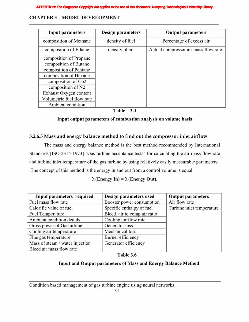
CHAPTER 3 – MODEL DEVELOPMENT _____________________________________________________________________________________________
Input parameters Design parameters Output parameters
composition of Methane density of fuel Percentage of excess air
composition of Ethane density of air Actual compressor air mass flow rate.
composition of Propane composition of Butane composition of Pentane composition of Hexane
composition of Co2 composition of N2
Exhaust Oxygen content Volumetric fuel flow rate
Ambient condition
Table – 3.4
Input output parameters of combustion analysis on volume basis
3.2.6.5 Mass and energy balance method to find out the compressor inlet airflow
The mass and energy balance method is the best method recommended by International
Standards [ISO 2314-1973] "Gas turbine acceptance tests" for calculating the air mass flow rate
and turbine inlet temperature of the gas turbine by using relatively easily measurable parameters.
The concept of this method is the energy in and out from a control volume is equal.
∑(Energy In) = ∑(Energy Out).
Input parameters required Design parameters used Output parameters Fuel mass flow rate Booster power consumption Air flow rate Calorific value of fuel Specific enthalpy of fuel Turbine inlet temperature Fuel Temperature Bleed air to comp air ratio Ambient condition details Cooling air flow rate Gross power of Gasturbine Generator loss Cooling air temperature Mechanical loss Flue gas temperature Burner efficiency Mass of steam / water injection Generator efficiency Bleed air mass flow rate
Table 3.6
Input and Output parameters of Mass and Energy Balance Method
Condition based management of gas turbine engine using neural networks 63
ATTENTION: The Singapore Copyright Act applies to the use of this document. Nanyang Technological University Library
CHAPTER 3 – MODEL DEVELOPMENT _____________________________________________________________________________________________
The data for this research work has been taken from single shaft gas turbine. The mass
and energy balance method has been tuned to suit this single shaft machine. Appendix A10
explains this method. Matlab program has been written [Math Works Inc, (2000a)] for
determining the air mass flow rate and turbine inlet temperature. It has been illustrated in
appendix B4. Input, design and output parameters of this model are given in table 3.6.
Table 3.7 in appendix C4 shows the comparison of the air inlet flow calculated using the Mass
and energy balance method with OEM’s values. These OEM’s airflow rate calculation has been
done before PAC test to set the gas turbine control functions.
The percentage of error between the airflow rate value calculated by using the mass &
energy balance method and OEM’s value is around 1.7%, which is quite low when compared to
the error of about 3.5% to 5.0% obtained in the exhaust O2 analysis method. This shows mass
and energy balance method is the best method for calculating the inlet air mass flow rate of gas
turbine by using relatively easily measurable parameters in the site. Table 3.8 in appendix C5
represents the inputs and outputs for the above thermodynamic model at various EOH.
3.3 Compressor washing details The compressor on-line washing, off-line washing and manual IGV blade cleaning
activities are noted for about 18000 EOH hours. Refer to table 3.9 in appendix A11 for details
regarding the compressor washings.
Condition based management of gas turbine engine using neural networks 64
ATTENTION: The Singapore Copyright Act applies to the use of this document. Nanyang Technological University Library
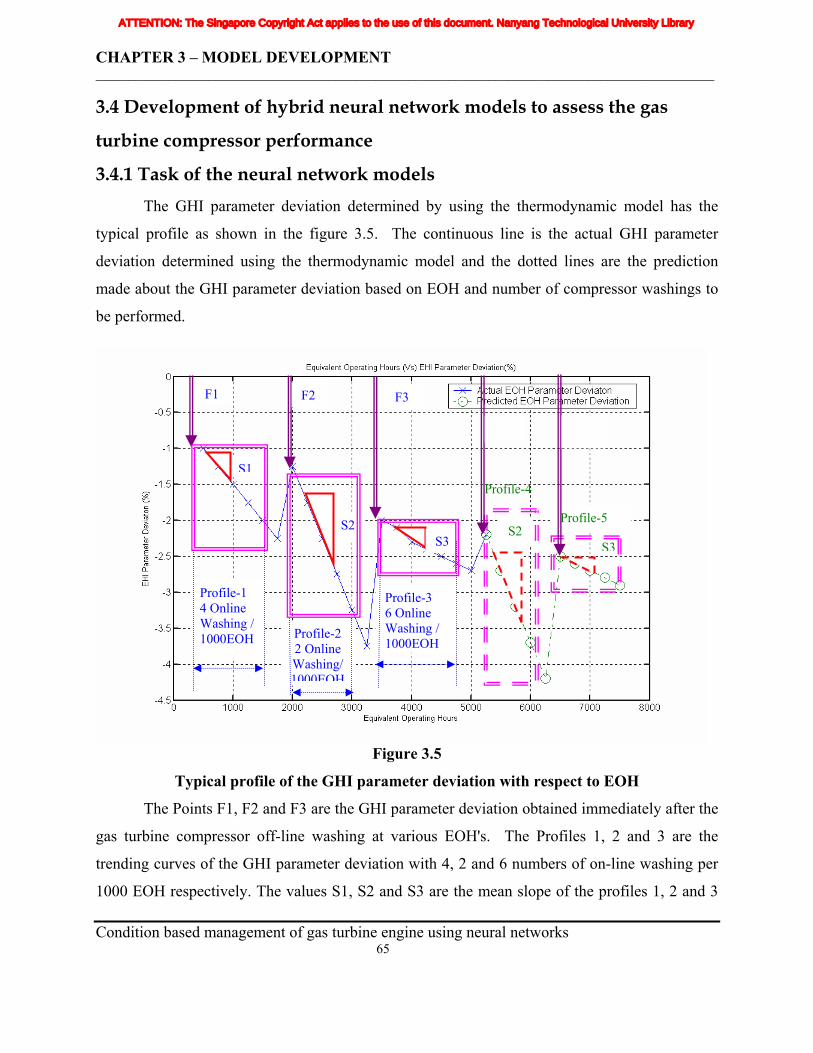
CHAPTER 3 – MODEL DEVELOPMENT _____________________________________________________________________________________________
3.4 Development of hybrid neural network models to assess the gas
turbine compressor performance
3.4.1 Task of the neural network models The GHI parameter deviation determined by using the thermodynamic model has the
typical profile as shown in the figure 3.5. The continuous line is the actual GHI parameter
deviation determined using the thermodynamic model and the dotted lines are the prediction
made about the GHI parameter deviation based on EOH and number of compressor washings to
be performed.
Profile-5
Profile-4
Profile-2 2 Online Washing/ 1000EOH
Profile-3 6 Online Washing / 1000EOH
Profile-1 4 Online Washing / 1000EOH
S3S2
S3S2
S1
F3 F2 F1
Figure 3.5
Typical profile of the GHI parameter deviation with respect to EOH
The Points F1, F2 and F3 are the GHI parameter deviation obtained immediately after the
gas turbine compressor off-line washing at various EOH's. The Profiles 1, 2 and 3 are the
trending curves of the GHI parameter deviation with 4, 2 and 6 numbers of on-line washing per
1000 EOH respectively. The values S1, S2 and S3 are the mean slope of the profiles 1, 2 and 3 Condition based management of gas turbine engine using neural networks 65
ATTENTION: The Singapore Copyright Act applies to the use of this document. Nanyang Technological University Library
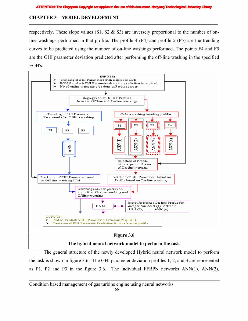
CHAPTER 3 – MODEL DEVELOPMENT _____________________________________________________________________________________________
respectively. These slope values (S1, S2 & S3) are inversely proportional to the number of on-
line washings performed in that profile. The profile 4 (P4) and profile 5 (P5) are the trending
curves to be predicted using the number of on-line washings performed. The points F4 and F5
are the GHI parameter deviation predicted after performing the off-line washing in the specified
EOH's.
Figure 3.6
The hybrid neural network model to perform the task
The general structure of the newly developed Hybrid neural network model to perform
the task is shown in figure 3.6. The GHI parameter deviation profiles 1, 2, and 3 are represented
as P1, P2 and P3 in the figure 3.6. The individual FFBPN networks ANN(1), ANN(2),
Condition based management of gas turbine engine using neural networks 66
ATTENTION: The Singapore Copyright Act applies to the use of this document. Nanyang Technological University Library
CHAPTER 3 – MODEL DEVELOPMENT _____________________________________________________________________________________________
ANN(3)… ANN(n) are developed for all the individual profiles P1, P2, P3… Pn based on
different on-line washing frequency per 1000EOH. The GHI parameter deviation obtained after
the off-line washing F1, F2, F3 are used to develop the FFBPN network ANN(0).
Based on the no of on-line washing to be performed in the prediction profile, the suitable
FFBPN network from ANN(1), ANN(2), ANN(3) … ANN(N) is selected. This selected FFBFN
network has been inputted with the range of EOH for which the prediction to be made. The
output of this network gives the GHI parameter deviation corresponding to the new EOH
inputted to the network. The time period where the new off-line washing line to performed has
to be inputted to the ANN(0) network and this ANN(0) network gives the corresponding GHI
parameter deviation after that particular of-fline washing. This prediction depends on the
trending of the points F1, F2, F3 and their EOH's. The results of the predicted GHI parameter
deviation obtained from selected ANN(n) and ANN(0) are merged together to obtained the
profiles P4 and P5. The mean slope of the predicted profiles P4 and P5 have been computed and
compared with the mean slope of the selected reference profile using PNN network. The output
of the PNN gives the details about the deviation of the predicted GHI parameter deviation from
the reference GHI parameter. [Leusden, Sorgenfrey and Lutz Dummel (2003),]
3.4.2 Gas turbine compressor performance modeling using hybrid neural networks
The Matlab neural network toolbox is equipped with a host of network structures and
neural functions, which along with the user's manual provides a very broad perspective in the art
of neural programming. The Hybrid neural network is used for the design and evaluation of the
gas turbine compressor performance model. The general structure of the newly developed
Hybrid neural network model to perform the task is shown in figure 3.6
The Inter-module communications of several FFBFN networks, PNN networks and the
expert system makes the developed hybrid network model to replicate the complex gas turbine
degradation profile. This inter-module communication by shared data structures enables faster
runtime performance and allows more sophisticated messages to be passed. The use of feedback
enables the dynamic nature of the system. All the above makes the developed hybrid neural
network model more suitable to replicate the complex gas turbine degradation profile, its
Condition based management of gas turbine engine using neural networks 67
ATTENTION: The Singapore Copyright Act applies to the use of this document. Nanyang Technological University Library
CHAPTER 3 – MODEL DEVELOPMENT _____________________________________________________________________________________________
analysis and predictions. The hybrid neural network program has been structured to perform the
following tasks.
a. Recognize the training data presented,
b. Perform the necessary pre-processing of data,
c. Perform network training based on the variants of following - Training functions,
training methods, number of iterations, mean squared error goal, number of hidden
layers and neurons within such layers.
d. Generate a mean square error versus number of iteration graph.
e. Perform an internal simulation and generation of residual graph for verification.
f. Allows the user to proceed with use of generated neural network model to simulate
other engine operating scenarios.
3.4.2.1 Flow Diagram of the Hybrid Neural network model
The flow diagram shown in figure 3.7 explains details about the logic and steps involved
in the new hybrid neural network model developed using the matlab toolbox.
The number of sets of reading for analyzing the on-line washing, off-line washing and
number of GHI parameter deviation to be monitored are given as input to the program.
Loop-A is created based on the number of on-line washing profiles to be analyzed. The
individual profiles GHI parameter deviations and their corresponding EOH are inputted in matrix
format inside this for loop. Similar approach has been followed and Loop-B is created to transfer
input regarding the off-line washing profile to be analyzed. Then the details regarding the
maximum EOH up to which prediction to be performed, frequency of the period of the
prediction, number of off-line washings to be done and when these off-line washings to be done
are inputted to the program (Loop-C1). Based on the maximum EOH upto which prediction to
made and number of off-line washings to performed, the number of off-line washing profile set
and their corresponding EOH are determined. (Loop C2).
Condition based management of gas turbine engine using neural networks 68
ATTENTION: The Singapore Copyright Act applies to the use of this document. Nanyang Technological University Library
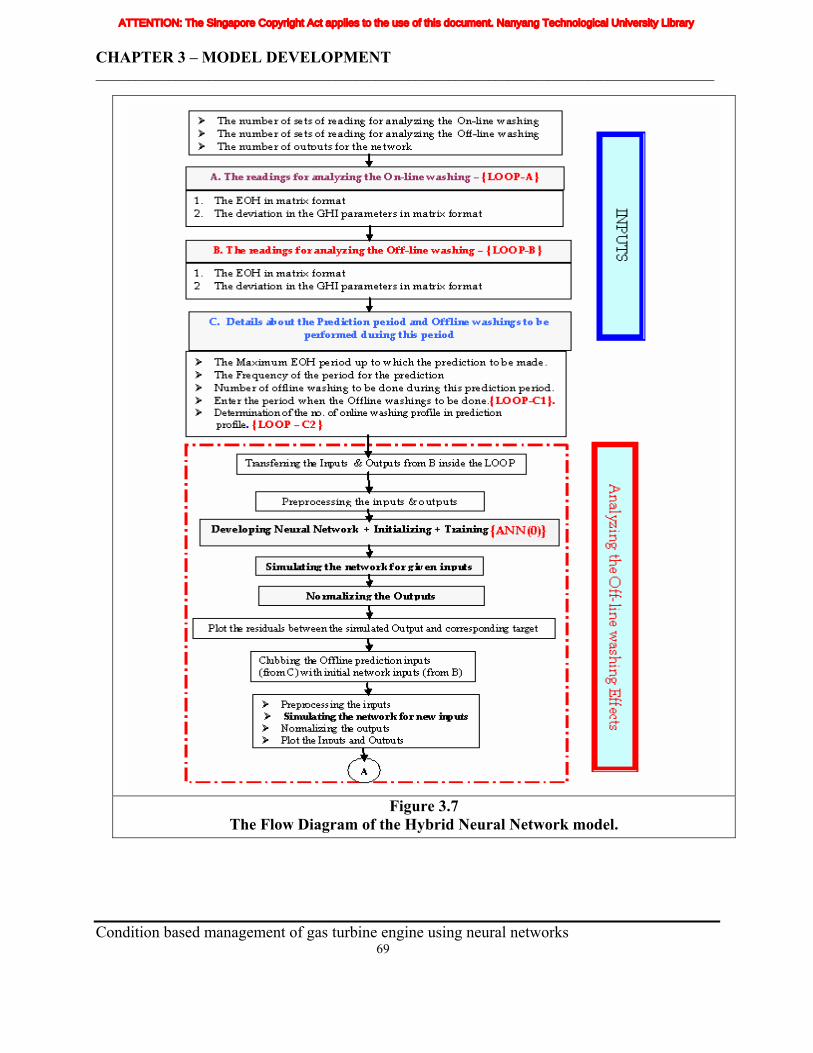
CHAPTER 3 – MODEL DEVELOPMENT _____________________________________________________________________________________________
Figure 3.7
The Flow Diagram of the Hybrid Neural Network model.
Condition based management of gas turbine engine using neural networks 69
ATTENTION: The Singapore Copyright Act applies to the use of this document. Nanyang Technological University Library
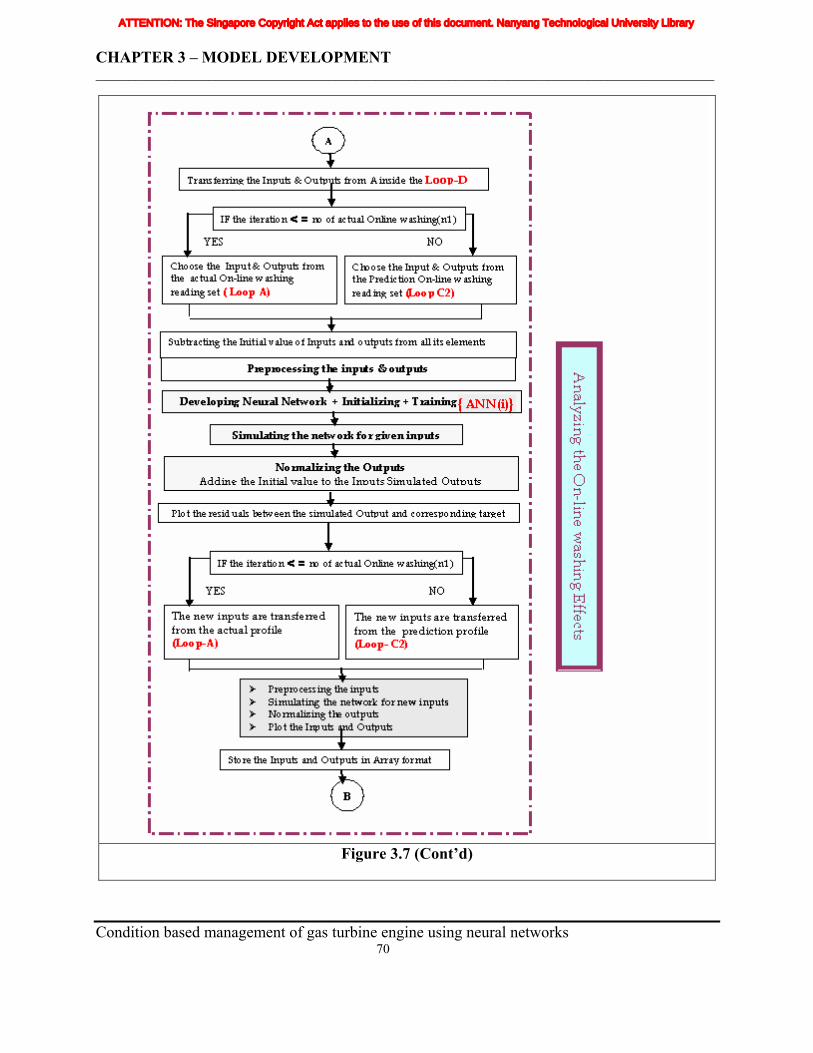
CHAPTER 3 – MODEL DEVELOPMENT _____________________________________________________________________________________________
Figure 3.7 (Cont’d)
Condition based management of gas turbine engine using neural networks 70
ATTENTION: The Singapore Copyright Act applies to the use of this document. Nanyang Technological University Library
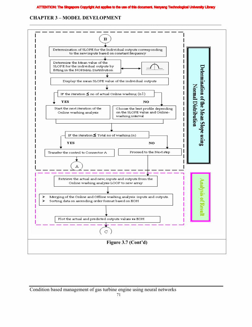
CHAPTER 3 – MODEL DEVELOPMENT _____________________________________________________________________________________________
Figure 3.7 (Cont’d)
Condition based management of gas turbine engine using neural networks 71
ATTENTION: The Singapore Copyright Act applies to the use of this document. Nanyang Technological University Library
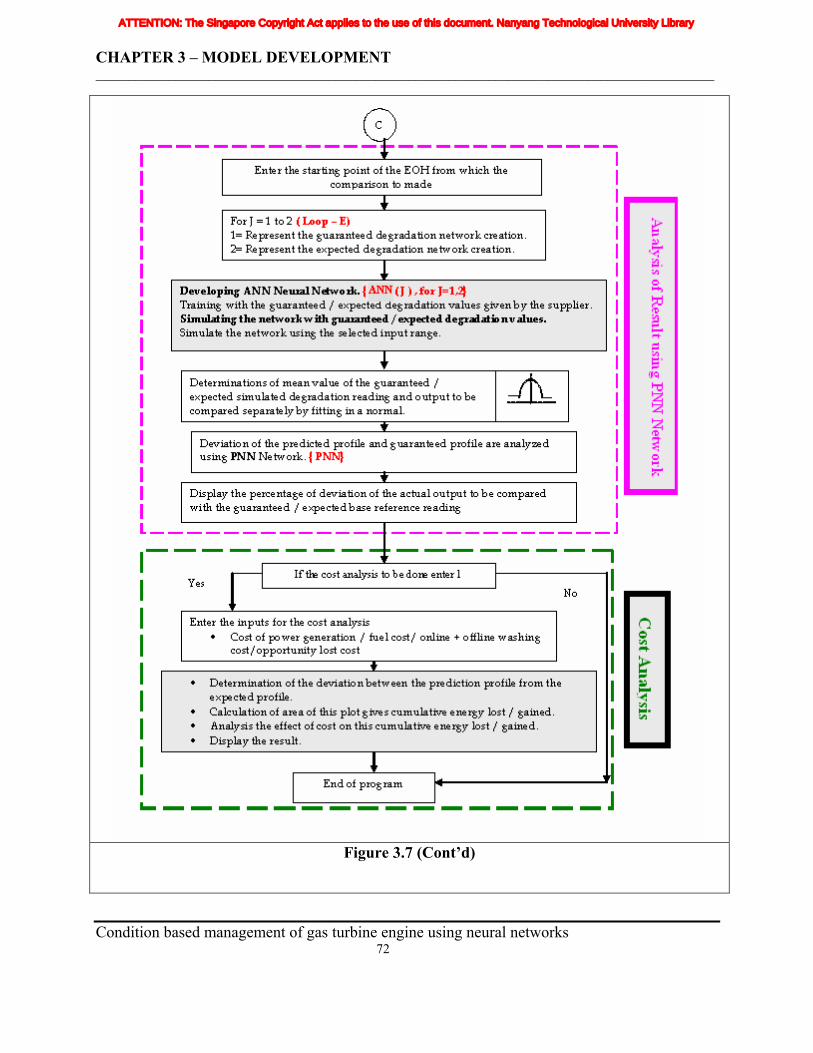
CHAPTER 3 – MODEL DEVELOPMENT _____________________________________________________________________________________________
Figure 3.7 (Cont’d)
Condition based management of gas turbine engine using neural networks 72
ATTENTION: The Singapore Copyright Act applies to the use of this document. Nanyang Technological University Library
CHAPTER 3 – MODEL DEVELOPMENT _____________________________________________________________________________________________
After receiving all the above inputs, the EOH and GHI parameter deviations
corresponding to off-line washing have been retrieved from Loop-B and used for analyzing the
off-line washing effects. These inputs and targets are preprocessed in order to make the neural
network training more efficient. A feed-forward backpropagation network ANN(0) is created by
using the function “newff” in the following manner.
eg. { net1=newff([uq2 uq4],[1,u1u],{'tansig','purelin'},'trainrp'); }
The values of the first element ranges from “uq2” ( min value of the EOH) and “uq4”
(max value of the EOH). The first layer (input) in the network has one neuron and the second
layer (output) of the network consist of “u1u” (number of GHI parameter deviations to be
monitored) neurons. The transfer function of the first layer is tan-sigmoid and the output layer is
pure linear. The training function used is Resilient back-propagation “trainrp” It is a simple
batch mode training algorithm with fast convergence and minimal storage requirements.
The ANN(0) network’s weights and biases are initialized and trained using the
normalized inputs and targets. This ANN(0) network is simulated and its outputs are normalized
using post-processing techniques. The residuals between the simulated outputs and
corresponding targets have been plotted. The off-line washing EOH period in the prediction
profile are retrieved from Loop-C1 and these inputs are normalized using the preprocessing
techniques. The network ANN(0) is simulated using the new normalized inputs and its outputs
are normalized using post-processing techniques. These outputs are stored in array format.
The EOH and GHI parameter deviations corresponding to the off-line washing have been
retrieved from Loop-A and it is used for analyzing the on-line washing effects. A new
“For Loop” (Loop-D) has been created with maximum iteration (n) equivalent to sum of actual
(n1) and prediction (n2) on-line profile sets. The conditional command “IF” is used to check the
number of iterations performed. If it is less than the actual on-line washing profile set, then the
particular actual on-line washing profile (from Loop-A) is selected as reference profile,
otherwise the particular prediction on-line washing profile (Loop-C2) is selected as reference
profile. A new feed-forward network ANN(i) is created. (where i=1 ,2 ,3 …… n {actual +
prediction profiles}). These feed-forward networks are also initialized, trained, simulated and
normalized in the same way like ANN(0) (ie feed forward created for analyzing the off-line
Condition based management of gas turbine engine using neural networks 73
ATTENTION: The Singapore Copyright Act applies to the use of this document. Nanyang Technological University Library
CHAPTER 3 – MODEL DEVELOPMENT _____________________________________________________________________________________________
washing effects). The inputs for simulating the ANN(i) network is taken based on the iteration
number. If the iteration number is less than the actual number of on-line profile set, then the
inputs are retrieved from actual on-line profile(Loop-A), otherwise inputs are taken from the
prediction on-line profile set.(Loop-C2). After simulation the outputs are normalized and stored
in array format.
The slopes of the outputs (GHI Parameter deviation) have been determined by using the
ratio of the deviation between the two successive outputs to their corresponding EOH deviations.
These slope values have been fitted in a normal distribution and its mean value is calculated. If
the current iteration is less than n1, then it transfers the control to the next step, otherwise it will
opt the user to select on-line washing profile to kept as reference for the next iteration. After
receiving the selection from the user, the program would check whether the current iteration is
less n (actual + prediction profile). If the current iteration is less n then it transfers the control to
the starting of the on-line washing effect analysis part of the program, otherwise it transfers the
control to the next part of the program. This part of the program shows the usage of several feed-
forward networks and the rule based modules without any changes regarding the conceptual
operation of either the neural network or rule based modules. It falls into the classification of
Modular hybrid neural system.
The predicted on-line washing inputs (EOH) and outputs (GHI parameter deviation) have
been retrieved from the above part of the program and merged with the predicted offline washing
inputs (EOH) and outputs (GHI parameter deviation). Sorting of the outputs in ascending order
have been done based on the EOH. The actual and predicted profile outputs (GHI parameter
deviation) have been plotted against their respective EOHs.
In this part, the EOH from which the comparison is to be made with the guaranteed
degradation value has to be inputted to the program. A new “For Loop” (Loop-E) has been
created with a maximum iteration value of 2. New feed-forward network, ANN (J) has been
created. (J=1, represent the network corresponding to the guaranteed design GHI degradation
value and J=2, represent the expected GHI degradation values.) . This network has been
initialized, trained and simulated using the predicted EOH same like previous networks. The
Condition based management of gas turbine engine using neural networks 74
ATTENTION: The Singapore Copyright Act applies to the use of this document. Nanyang Technological University Library
CHAPTER 3 – MODEL DEVELOPMENT _____________________________________________________________________________________________
GHI outputs of this network is normalized and fitted into normal distribution. The mean value of
this distribution is determined and stored.
A PNN network has been created to analysis the deviation between the predicted GHI
parameters deviation with the guaranteed and expected GHI parameters deviation.
Cost of power generation, fuel cost, on-line & off-line washing cost and opportunity lost
cost have to be inputted to the program. Refer to Table 4.18 and 4.19 in the appendix-D2 for the
details regarding the above cost. The plot has been made between expected GHI parameter
deviations with the predicted GHI parameter deviation. The algebraic sum of this curve area
gives the cumulative energy lost or gained. Effects of the cost factors on the cumulative energy
lost or gained have been done and result is displayed.
3.4.2.2 Matlab programming structure of the Hybrid Neural Network modeling
The detail logic of this hybrid neural network program has been explained in the
figure 3.7. Kindly refer the appendix B4 for the hybrid matlab programming to assess the gas
turbine engine health condition using prestd preprocessing technique. In this program the data
are processed by prestd preprocessing and postprocessing techniques.
Preprocessing [pn,meanp,stdp,tn,meant,stdt]=prestd(p,t);
Network creation
net = train (net, pn, tn);
an = sim(net,pn)
Post processing
a = poststd( an, meant, stdt);
pnewn =trastd(pnew,meanp,stdp);
Simulation with new inputs
anewn=sim(net,pnewn);
Post processing
anew =poststd(anew,meant,stdt);
Condition based management of gas turbine engine using neural networks 75
ATTENTION: The Singapore Copyright Act applies to the use of this document. Nanyang Technological University Library
CHAPTER 3 – MODEL DEVELOPMENT _____________________________________________________________________________________________
Condition based management of gas turbine engine using neural networks 76
In the same way the matlab programming has been written for processing the data using
preminmax technique also. The program structure is same like the above steps, only the
codification of preprocessing, simulation and post processing steps would be as follows,
Preprocessing
[pn, minp, maxp,tn,mint, maxt] = premnmx(p,t);
Network creation
net = train(net, pn, tn);
an = sim(net,pn);
Post processing
a = postmnmx(an, mint, maxt);
pnewn = tramnmx(pnew, minp, maxp);
Simulation with new inputs
anewn = sim(net, pnewn);
Post processing
anew = postmnmx( anewn, mint, maxt);
The matlab program for directly using the raw data has also been written in the similar
and it would not consist of any preprocessing and post processing steps.
Network creation
net = train(net, p, t);
Simulation
Anew=sim(net,pnew);
All the above three models are used for analyzing for gas turbine health assessment program.
ATTENTION: The Singapore Copyright Act applies to the use of this document. Nanyang Technological University Library
CHAPTER 4 – RESULTS & DISCUSSIONS ______________________________________________________________________________
4.1 Overview of thermodynamic model results The outputs of the thermodynamic models have been analyzed in the following manner:-
• Analysis of the general curve profile of EHI Parameters.
• Curve fitting of the PAC test results.
• Analysis of the long term trending of EHI Parameters.
• Comparison of OEM and STD correction effects on EHI parameter trending.
4.1.1 Analysis of general curve profiles of EHI Parameters The general profile of the CCPP gross efficiency has been studied under different
circumstances. It has been plotted against CCPP corrected gross load based on OEM corrections,
STD corrections, PAC test result and guaranteed curve. Figure 4.1 shows the profile of the CCPP
gross thermal efficiency under the above four different circumstances.
In the figure 4.1 the gross thermal efficiency is plotted on the ordinate and CCPP gross load
is plotted on the abscissa. The gross thermal efficiency increases with the increase of the CCPP
gross load. The gradient of the gross thermal efficiency increase is higher from 220MW (60%) to
350MW (93%) of CCPP gross load when compared with CCPP gross load of above
350MW(>93%). This difference arises due to the change in the gas turbine controller from IGV
mode to OTC mode. In the IGV mode the air flow rate is increased in proportion to the increase
of the fuel flow rate and air/fuel ratio is maintained at optimum value. When the IGV reaches its
maximum opening position the controller switches to OTC mode. In OTC control mode the fuel
flow rate alone is increased until the turbine inlet temperature reaches 1250°C. This increased
fuel flow reduces the gradient of gross thermal efficiency increase above 350MW (>93%) CCPP
gross load. The figure 4.1 shows similar behavior of gross thermal efficiency when it is plotted
against CCPP corrected gross load based on OEM corrections, STD corrections, PAC test result
and guaranteed curve. The variation of gross thermal efficiency based on OEM corrections, STD
corrections and PAC test result are within 0.5% and they are greater than 1.5% to 2.0% from the
guaranteed curve. This analysis has been done as a part of verification of the developed
thermodynamic models with actual system.
______________________________________________________________________________ Condition based management of gas turbine engine using neural networks 77
ATTENTION: The Singapore Copyright Act applies to the use of this document. Nanyang Technological University Library
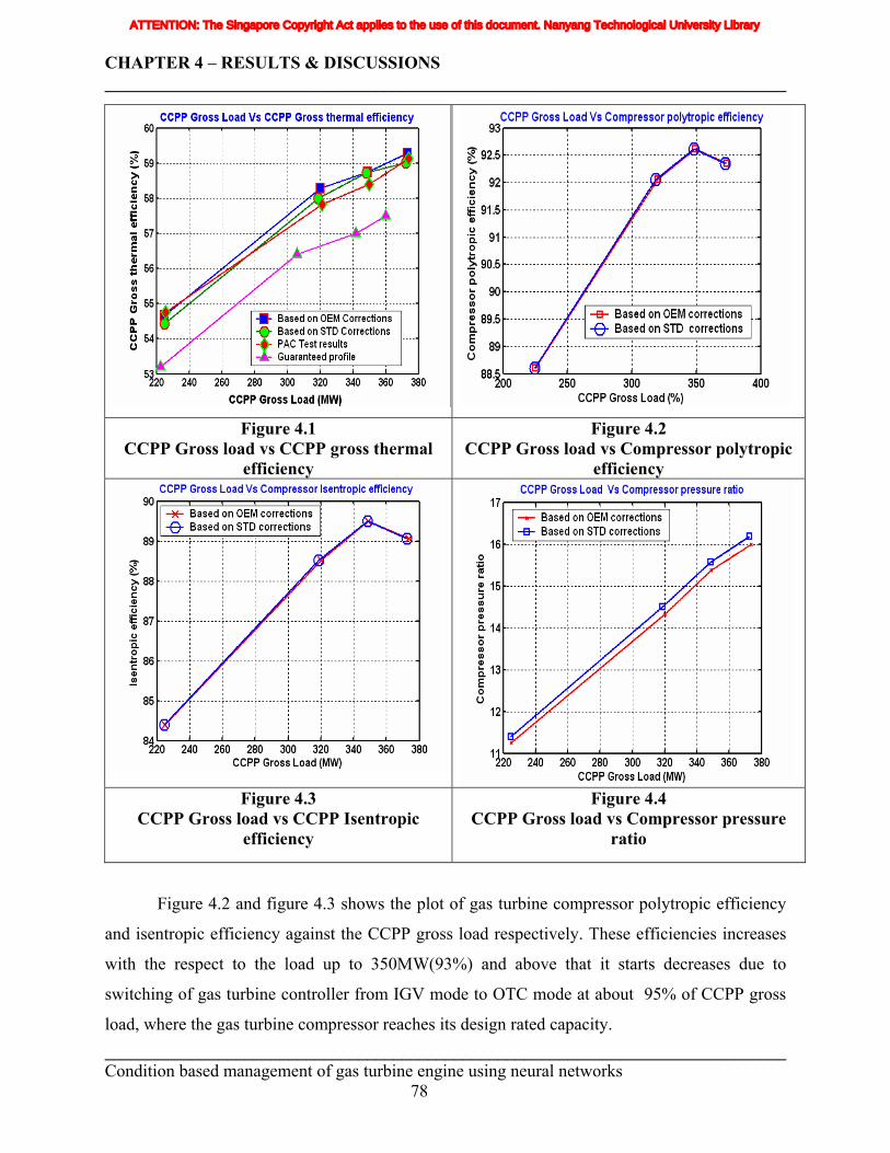
CHAPTER 4 – RESULTS & DISCUSSIONS ______________________________________________________________________________
Figure 4.1
CCPP Gross load vs CCPP gross thermal efficiency
Figure 4.2 CCPP Gross load vs Compressor polytropic
efficiency
Figure 4.3
CCPP Gross load vs CCPP Isentropic efficiency
Figure 4.4 CCPP Gross load vs Compressor pressure
ratio
Figure 4.2 and figure 4.3 shows the plot of gas turbine compressor polytropic efficiency
and isentropic efficiency against the CCPP gross load respectively. These efficiencies increases
with the respect to the load up to 350MW(93%) and above that it starts decreases due to
switching of gas turbine controller from IGV mode to OTC mode at about 95% of CCPP gross
load, where the gas turbine compressor reaches its design rated capacity. ______________________________________________________________________________ Condition based management of gas turbine engine using neural networks 78
ATTENTION: The Singapore Copyright Act applies to the use of this document. Nanyang Technological University Library
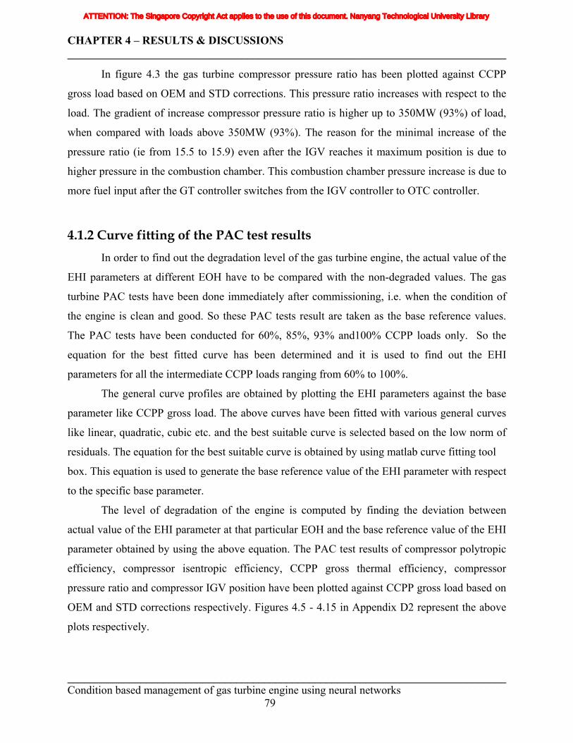
CHAPTER 4 – RESULTS & DISCUSSIONS ______________________________________________________________________________
In figure 4.3 the gas turbine compressor pressure ratio has been plotted against CCPP
gross load based on OEM and STD corrections. This pressure ratio increases with respect to the
load. The gradient of increase compressor pressure ratio is higher up to 350MW (93%) of load,
when compared with loads above 350MW (93%). The reason for the minimal increase of the
pressure ratio (ie from 15.5 to 15.9) even after the IGV reaches it maximum position is due to
higher pressure in the combustion chamber. This combustion chamber pressure increase is due to
more fuel input after the GT controller switches from the IGV controller to OTC controller.
4.1.2 Curve fitting of the PAC test results In order to find out the degradation level of the gas turbine engine, the actual value of the
EHI parameters at different EOH have to be compared with the non-degraded values. The gas
turbine PAC tests have been done immediately after commissioning, i.e. when the condition of
the engine is clean and good. So these PAC tests result are taken as the base reference values.
The PAC tests have been conducted for 60%, 85%, 93% and100% CCPP loads only. So the
equation for the best fitted curve has been determined and it is used to find out the EHI
parameters for all the intermediate CCPP loads ranging from 60% to 100%.
The general curve profiles are obtained by plotting the EHI parameters against the base
parameter like CCPP gross load. The above curves have been fitted with various general curves
like linear, quadratic, cubic etc. and the best suitable curve is selected based on the low norm of
residuals. The equation for the best suitable curve is obtained by using matlab curve fitting tool
box. This equation is used to generate the base reference value of the EHI parameter with respect
to the specific base parameter.
The level of degradation of the engine is computed by finding the deviation between
actual value of the EHI parameter at that particular EOH and the base reference value of the EHI
parameter obtained by using the above equation. The PAC test results of compressor polytropic
efficiency, compressor isentropic efficiency, CCPP gross thermal efficiency, compressor
pressure ratio and compressor IGV position have been plotted against CCPP gross load based on
OEM and STD corrections respectively. Figures 4.5 - 4.15 in Appendix D2 represent the above
plots respectively.
______________________________________________________________________________ Condition based management of gas turbine engine using neural networks 79
ATTENTION: The Singapore Copyright Act applies to the use of this document. Nanyang Technological University Library
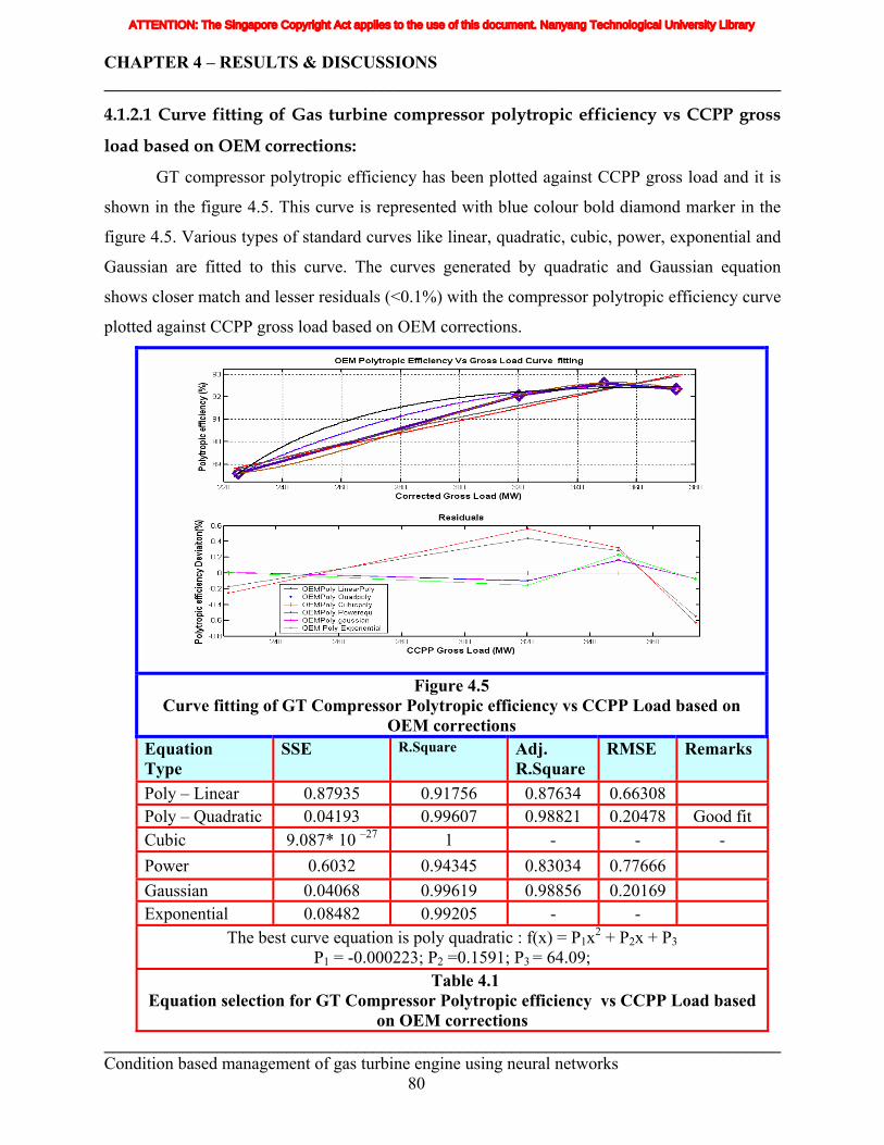
CHAPTER 4 – RESULTS & DISCUSSIONS ______________________________________________________________________________
4.1.2.1 Curve fitting of Gas turbine compressor polytropic efficiency vs CCPP gross
load based on OEM corrections:
GT compressor polytropic efficiency has been plotted against CCPP gross load and it is
shown in the figure 4.5. This curve is represented with blue colour bold diamond marker in the
figure 4.5. Various types of standard curves like linear, quadratic, cubic, power, exponential and
Gaussian are fitted to this curve. The curves generated by quadratic and Gaussian equation
shows closer match and lesser residuals (<0.1%) with the compressor polytropic efficiency curve
plotted against CCPP gross load based on OEM corrections.
______________________________________________________________________________ Condition based management of gas turbine engine using neural networks 80
Figure 4.5 Curve fitting of GT Compressor Polytropic efficiency vs CCPP Load based on
OEM corrections Equation Type
SSE R.Square Adj. R.Square
RMSE Remarks
Poly – Linear 0.87935 0.91756 0.87634 0.66308 Poly – Quadratic 0.04193 0.99607 0.98821 0.20478 Good fit Cubic 9.087* 10 –27 1 - - - Power 0.6032 0.94345 0.83034 0.77666 Gaussian 0.04068 0.99619 0.98856 0.20169 Exponential 0.08482 0.99205 - -
The best curve equation is poly quadratic : f(x) = P1x2 + P2x + P3 P1 = -0.000223; P2 =0.1591; P3 = 64.09;
Table 4.1 Equation selection for GT Compressor Polytropic efficiency vs CCPP Load based
on OEM corrections
ATTENTION: The Singapore Copyright Act applies to the use of this document. Nanyang Technological University Library
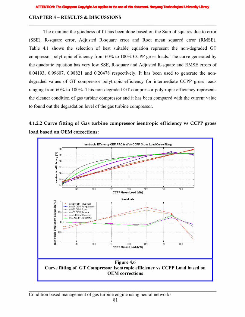
CHAPTER 4 – RESULTS & DISCUSSIONS ______________________________________________________________________________
The examine the goodness of fit has been done based on the Sum of squares due to error
(SSE), R-square error, Adjusted R-square error and Root mean squared error (RMSE).
Table 4.1 shows the selection of best suitable equation represent the non-degraded GT
compressor polytropic efficiency from 60% to 100% CCPP gross loads. The curve generated by
the quadratic equation has very low SSE, R-square and Adjusted R-square and RMSE errors of
0.04193, 0.99607, 0.98821 and 0.20478 respectively. It has been used to generate the non-
degraded values of GT compressor polytropic efficiency for intermediate CCPP gross loads
ranging from 60% to 100%. This non-degraded GT compressor polytropic efficiency represents
the cleaner condition of gas turbine compressor and it has been compared with the current value
to found out the degradation level of the gas turbine compressor.
4.1.2.2 Curve fitting of Gas turbine compressor isentropic efficiency vs CCPP gross
load based on OEM corrections:
Figure 4.6 Curve fitting of GT Compressor Isentropic efficiency vs CCPP Load based on
OEM corrections
______________________________________________________________________________ Condition based management of gas turbine engine using neural networks 81
ATTENTION: The Singapore Copyright Act applies to the use of this document. Nanyang Technological University Library
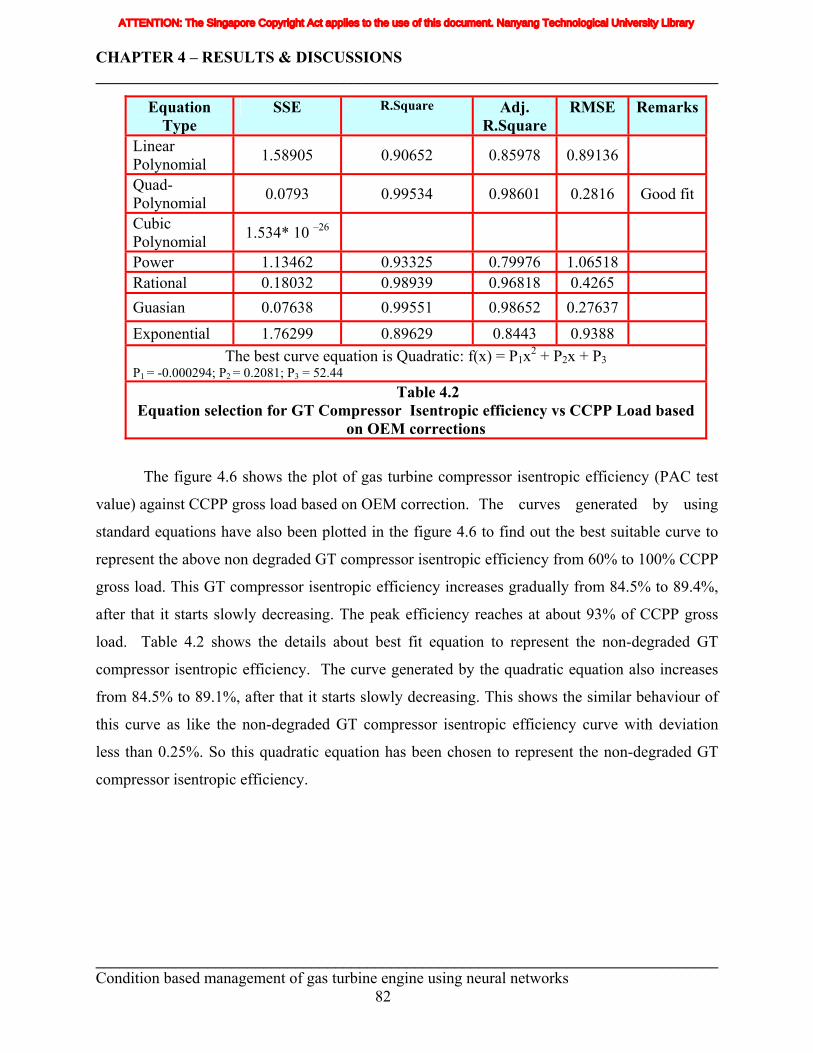
CHAPTER 4 – RESULTS & DISCUSSIONS ______________________________________________________________________________
Equation Type
SSE R.Square Adj. R.Square
RMSE Remarks
Linear Polynomial 1.58905 0.90652 0.85978 0.89136
Quad- Polynomial 0.0793 0.99534 0.98601 0.2816 Good fit
Cubic Polynomial 1.534* 10 –26
Power 1.13462 0.93325 0.79976 1.06518 Rational 0.18032 0.98939 0.96818 0.4265 Guasian 0.07638 0.99551 0.98652 0.27637 Exponential 1.76299 0.89629 0.8443 0.9388
The best curve equation is Quadratic: f(x) = P1x2 + P2x + P3 P1 = -0.000294; P2 = 0.2081; P3 = 52.44
Table 4.2 Equation selection for GT Compressor Isentropic efficiency vs CCPP Load based
on OEM corrections
The figure 4.6 shows the plot of gas turbine compressor isentropic efficiency (PAC test
value) against CCPP gross load based on OEM correction. The curves generated by using
standard equations have also been plotted in the figure 4.6 to find out the best suitable curve to
represent the above non degraded GT compressor isentropic efficiency from 60% to 100% CCPP
gross load. This GT compressor isentropic efficiency increases gradually from 84.5% to 89.4%,
after that it starts slowly decreasing. The peak efficiency reaches at about 93% of CCPP gross
load. Table 4.2 shows the details about best fit equation to represent the non-degraded GT
compressor isentropic efficiency. The curve generated by the quadratic equation also increases
from 84.5% to 89.1%, after that it starts slowly decreasing. This shows the similar behaviour of
this curve as like the non-degraded GT compressor isentropic efficiency curve with deviation
less than 0.25%. So this quadratic equation has been chosen to represent the non-degraded GT
compressor isentropic efficiency.
______________________________________________________________________________ Condition based management of gas turbine engine using neural networks 82
ATTENTION: The Singapore Copyright Act applies to the use of this document. Nanyang Technological University Library
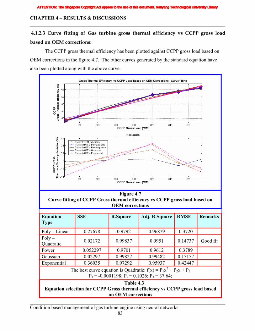
CHAPTER 4 – RESULTS & DISCUSSIONS ______________________________________________________________________________
4.1.2.3 Curve fitting of Gas turbine gross thermal efficiency vs CCPP gross load
based on OEM corrections:
The CCPP gross thermal efficiency has been plotted against CCPP gross load based on
OEM corrections in the figure 4.7. The other curves generated by the standard equation have
also been plotted along with the above curve.
______________________________________________________________________________ Condition based management of gas turbine engine using neural networks 83
Figure 4.7 Curve fitting of CCPP Gross thermal efficiency vs CCPP gross load based on
OEM corrections
Equation Type
SSE R.Square Adj. R.Square RMSE Remarks
Poly – Linear 0.27678 0.9792 0.96879 0.3720 Poly – Quadratic 0.02172 0.99837 0.9951 0.14737 Good fit
Power 0.052297 0.9701 0.9612 0.3789 Gaussian 0.02297 0.99827 0.99482 0.15157 Exponential 0.36035 0.97292 0.95937 0.42447
The best curve equation is Quadratic: f(x) = P1x2 + P2x + P3 P1 = -0.0001198; P2 = 0.1026; P3 = 37.64;
Table 4.3 Equation selection for CCPP Gross thermal efficiency vs CCPP gross load based
on OEM corrections
ATTENTION: The Singapore Copyright Act applies to the use of this document. Nanyang Technological University Library
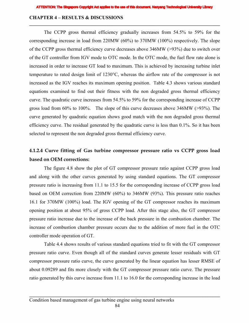
CHAPTER 4 – RESULTS & DISCUSSIONS ______________________________________________________________________________
The CCPP gross thermal efficiency gradually increases from 54.5% to 59% for the
corresponding increase in load from 220MW (60%) to 370MW (100%) respectively. The slope
of the CCPP gross thermal efficiency curve decreases above 346MW (>93%) due to switch over
of the GT controller from IGV mode to OTC mode. In the OTC mode, the fuel flow rate alone is
increased in order to increase GT load to maximum. This is achieved by increasing turbine inlet
temperature to rated design limit of 1230°C, whereas the airflow rate of the compressor is not
increased as the IGV reaches its maximum opening position. Table 4.3 shows various standard
equations examined to find out their fitness with the non degraded gross thermal efficiency
curve. The quadratic curve increases from 54.5% to 59% for the corresponding increase of CCPP
gross load from 60% to 100%. The slope of this curve decreases above 346MW (>93%). The
curve generated by quadratic equation shows good match with the non degraded gross thermal
efficiency curve. The residual generated by the quadratic curve is less than 0.1%. So it has been
selected to represent the non degraded gross thermal efficiency curve.
4.1.2.4 Curve fitting of Gas turbine compressor pressure ratio vs CCPP gross load
based on OEM corrections:
The figure 4.8 show the plot of GT compressor pressure ratio against CCPP gross load
and along with the other curves generated by using standard equations. The GT compressor
pressure ratio is increasing from 11.1 to 15.5 for the corresponding increase of CCPP gross load
based on OEM correction from 220MW (60%) to 346MW (93%). This pressure ratio reaches
16.1 for 370MW (100%) load. The IGV opening of the GT compressor reaches its maximum
opening position at about 95% of gross CCPP load. After this stage also, the GT compressor
pressure ratio increase due to the increase of the back pressure in the combustion chamber. The
increase of combustion chamber pressure occurs due to the addition of more fuel in the OTC
controller mode operation of GT.
Table 4.4 shows results of various standard equations tried to fit with the GT compressor
pressure ratio curve. Even though all of the standard curves generate lesser residuals with GT
compressor pressure ratio curve, the curve generated by the linear equation has lesser RMSE of
about 0.09289 and fits more closely with the GT compressor pressure ratio curve. The pressure
ratio generated by this curve increase from 11.1 to 16.0 for the corresponding increase in the load
______________________________________________________________________________ Condition based management of gas turbine engine using neural networks 84
ATTENTION: The Singapore Copyright Act applies to the use of this document. Nanyang Technological University Library
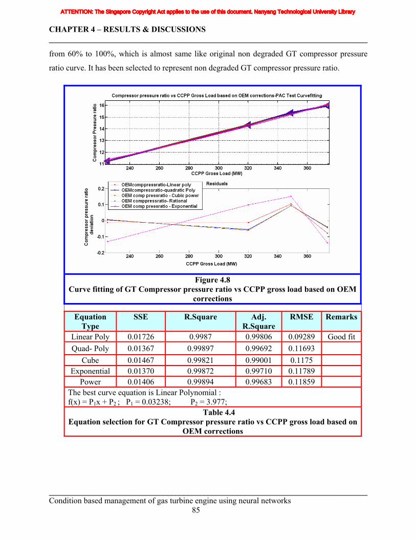
CHAPTER 4 – RESULTS & DISCUSSIONS ______________________________________________________________________________
from 60% to 100%, which is almost same like original non degraded GT compressor pressure
ratio curve. It has been selected to represent non degraded GT compressor pressure ratio.
Figure 4.8 Curve fitting of GT Compressor pressure ratio vs CCPP gross load based on OEM
corrections
Equation Type
SSE R.Square Adj. R.Square
RMSE Remarks
Linear Poly 0.01726 0.9987 0.99806 0.09289 Good fit Quad- Poly 0.01367 0.99897 0.99692 0.11693
Cube 0.01467 0.99821 0.99001 0.1175 Exponential 0.01370 0.99872 0.99710 0.11789
Power 0.01406 0.99894 0.99683 0.11859 The best curve equation is Linear Polynomial : f(x) = P1x + P2 ; P1 = 0.03238; P2 = 3.977;
Table 4.4 Equation selection for GT Compressor pressure ratio vs CCPP gross load based on
OEM corrections
______________________________________________________________________________ Condition based management of gas turbine engine using neural networks 85
ATTENTION: The Singapore Copyright Act applies to the use of this document. Nanyang Technological University Library
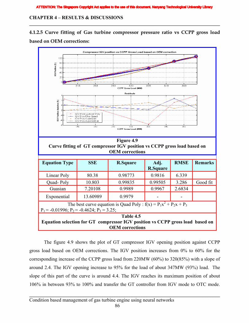
CHAPTER 4 – RESULTS & DISCUSSIONS ______________________________________________________________________________
4.1.2.5 Curve fitting of Gas turbine compressor pressure ratio vs CCPP gross load
based on OEM corrections:
Figure 4.9 Curve fitting of GT compressor IGV position vs CCPP gross load based on
OEM corrections
Equation Type SSE R.Square Adj. R.Square
RMSE Remarks
Linear Poly 80.38 0.98773 0.9816 6.339 Quad- Poly 10.803 0.99835 0.99505 3.286 Good fit
Guasian 7.20108 0.9989 0.9967 2.6834 Exponential 13.60989 0.9979 - -
The best curve equation is Quad Poly : f(x) = P1x2 + P2x + P3 P1 = -0.01996; P2 = -0.4624; P3 = 3.25;
Table 4.5 Equation selection for GT compressor IGV position vs CCPP gross load based on
OEM corrections
The figure 4.9 shows the plot of GT compressor IGV opening position against CCPP
gross load based on OEM corrections. The IGV position increases from 0% to 60% for the
corresponding increase of the CCPP gross load from 220MW (60%) to 320(85%) with a slope of
around 2.4. The IGV opening increase to 95% for the load of about 347MW (93%) load. The
slope of this part of the curve is around 4.4. The IGV reaches its maximum position of about
106% in between 93% to 100% and transfer the GT controller from IGV mode to OTC mode.
______________________________________________________________________________ Condition based management of gas turbine engine using neural networks 86
ATTENTION: The Singapore Copyright Act applies to the use of this document. Nanyang Technological University Library
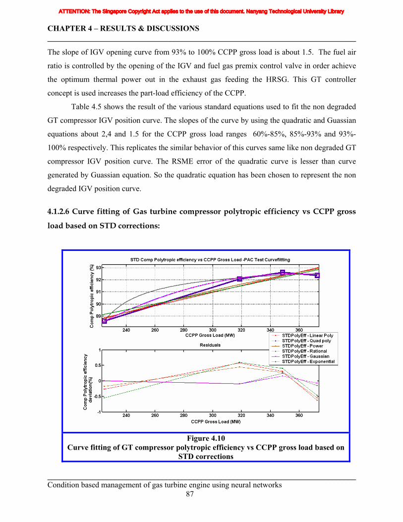
CHAPTER 4 – RESULTS & DISCUSSIONS ______________________________________________________________________________
The slope of IGV opening curve from 93% to 100% CCPP gross load is about 1.5. The fuel air
ratio is controlled by the opening of the IGV and fuel gas premix control valve in order achieve
the optimum thermal power out in the exhaust gas feeding the HRSG. This GT controller
concept is used increases the part-load efficiency of the CCPP.
Table 4.5 shows the result of the various standard equations used to fit the non degraded
GT compressor IGV position curve. The slopes of the curve by using the quadratic and Guassian
equations about 2,4 and 1.5 for the CCPP gross load ranges 60%-85%, 85%-93% and 93%-
100% respectively. This replicates the similar behavior of this curves same like non degraded GT
compressor IGV position curve. The RSME error of the quadratic curve is lesser than curve
generated by Guassian equation. So the quadratic equation has been chosen to represent the non
degraded IGV position curve.
4.1.2.6 Curve fitting of Gas turbine compressor polytropic efficiency vs CCPP gross
load based on STD corrections:
Figure 4.10 Curve fitting of GT compressor polytropic efficiency vs CCPP gross load based on
STD corrections
______________________________________________________________________________ Condition based management of gas turbine engine using neural networks 87
ATTENTION: The Singapore Copyright Act applies to the use of this document. Nanyang Technological University Library
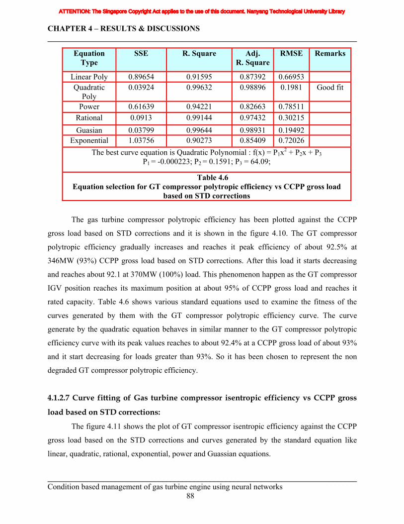
CHAPTER 4 – RESULTS & DISCUSSIONS ______________________________________________________________________________
Equation Type
SSE R. Square Adj. R. Square
RMSE Remarks
Linear Poly 0.89654 0.91595 0.87392 0.66953 Quadratic
Poly 0.03924 0.99632 0.98896 0.1981 Good fit
Power 0.61639 0.94221 0.82663 0.78511 Rational 0.0913 0.99144 0.97432 0.30215 Guasian 0.03799 0.99644 0.98931 0.19492
Exponential 1.03756 0.90273 0.85409 0.72026 The best curve equation is Quadratic Polynomial : f(x) = P1x2 + P2x + P3
P1 = -0.000223; P2 = 0.1591; P3 = 64.09;
Table 4.6 Equation selection for GT compressor polytropic efficiency vs CCPP gross load
based on STD corrections
The gas turbine compressor polytropic efficiency has been plotted against the CCPP
gross load based on STD corrections and it is shown in the figure 4.10. The GT compressor
polytropic efficiency gradually increases and reaches it peak efficiency of about 92.5% at
346MW (93%) CCPP gross load based on STD corrections. After this load it starts decreasing
and reaches about 92.1 at 370MW (100%) load. This phenomenon happen as the GT compressor
IGV position reaches its maximum position at about 95% of CCPP gross load and reaches it
rated capacity. Table 4.6 shows various standard equations used to examine the fitness of the
curves generated by them with the GT compressor polytropic efficiency curve. The curve
generate by the quadratic equation behaves in similar manner to the GT compressor polytropic
efficiency curve with its peak values reaches to about 92.4% at a CCPP gross load of about 93%
and it start decreasing for loads greater than 93%. So it has been chosen to represent the non
degraded GT compressor polytropic efficiency.
4.1.2.7 Curve fitting of Gas turbine compressor isentropic efficiency vs CCPP gross
load based on STD corrections:
The figure 4.11 shows the plot of GT compressor isentropic efficiency against the CCPP
gross load based on the STD corrections and curves generated by the standard equation like
linear, quadratic, rational, exponential, power and Guassian equations.
______________________________________________________________________________ Condition based management of gas turbine engine using neural networks 88
ATTENTION: The Singapore Copyright Act applies to the use of this document. Nanyang Technological University Library
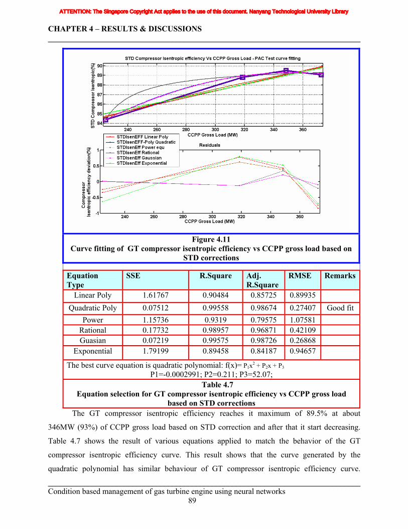
CHAPTER 4 – RESULTS & DISCUSSIONS ______________________________________________________________________________
Figure 4.11
Curve fitting of GT compressor isentropic efficiency vs CCPP gross load based on STD corrections
Equation Type
SSE R.Square Adj. R.Square
RMSE Remarks
Linear Poly 1.61767 0.90484 0.85725 0.89935 Quadratic Poly 0.07512 0.99558 0.98674 0.27407 Good fit
Power 1.15736 0.9319 0.79575 1.07581 Rational 0.17732 0.98957 0.96871 0.42109 Guasian 0.07219 0.99575 0.98726 0.26868
Exponential 1.79199 0.89458 0.84187 0.94657
The best curve equation is quadratic polynomial: f(x)= P1x2 + P2x + P3 P1=-0.0002991; P2=0.211; P3=52.07;
Table 4.7 Equation selection for GT compressor isentropic efficiency vs CCPP gross load
based on STD corrections The GT compressor isentropic efficiency reaches it maximum of 89.5% at about
346MW (93%) of CCPP gross load based on STD correction and after that it start decreasing.
Table 4.7 shows the result of various equations applied to match the behavior of the GT
compressor isentropic efficiency curve. This result shows that the curve generated by the
quadratic polynomial has similar behaviour of GT compressor isentropic efficiency curve.
______________________________________________________________________________ Condition based management of gas turbine engine using neural networks 89
ATTENTION: The Singapore Copyright Act applies to the use of this document. Nanyang Technological University Library
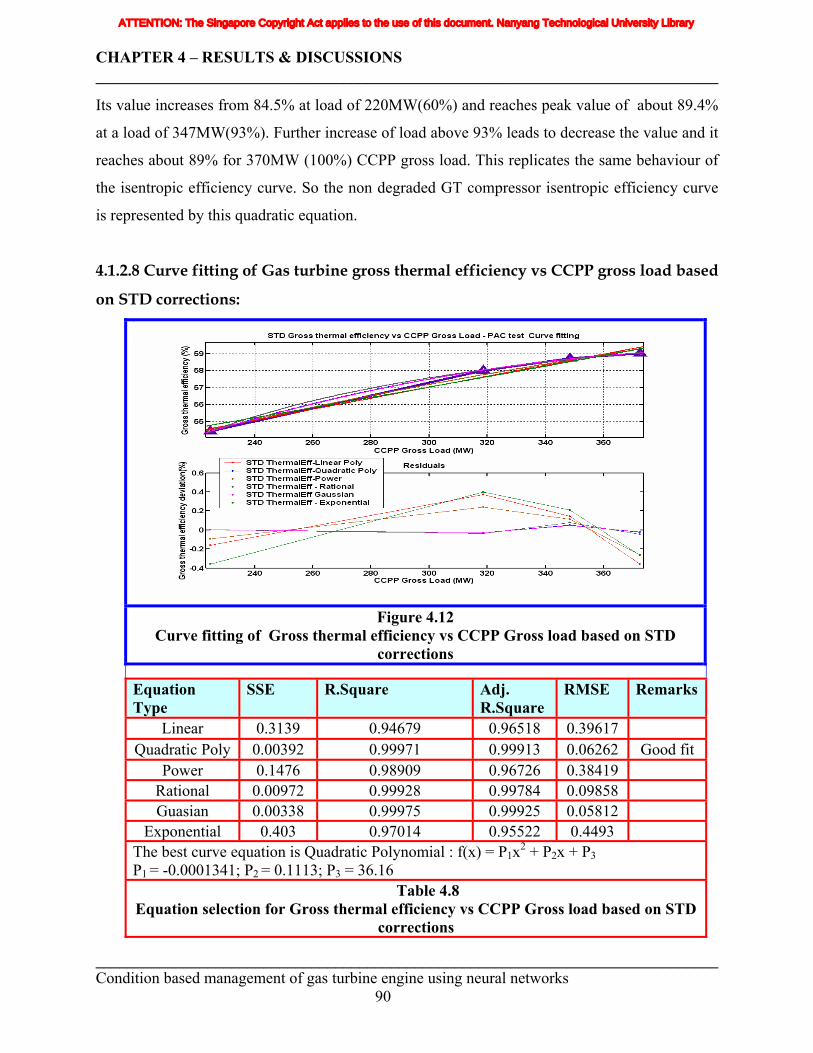
CHAPTER 4 – RESULTS & DISCUSSIONS ______________________________________________________________________________
Its value increases from 84.5% at load of 220MW(60%) and reaches peak value of about 89.4%
at a load of 347MW(93%). Further increase of load above 93% leads to decrease the value and it
reaches about 89% for 370MW (100%) CCPP gross load. This replicates the same behaviour of
the isentropic efficiency curve. So the non degraded GT compressor isentropic efficiency curve
is represented by this quadratic equation.
4.1.2.8 Curve fitting of Gas turbine gross thermal efficiency vs CCPP gross load based
on STD corrections:
Figure 4.12 Curve fitting of Gross thermal efficiency vs CCPP Gross load based on STD
corrections
Equation Type
SSE R.Square Adj. R.Square
RMSE Remarks
Linear 0.3139 0.94679 0.96518 0.39617 Quadratic Poly 0.00392 0.99971 0.99913 0.06262 Good fit
Power 0.1476 0.98909 0.96726 0.38419 Rational 0.00972 0.99928 0.99784 0.09858 Guasian 0.00338 0.99975 0.99925 0.05812
Exponential 0.403 0.97014 0.95522 0.4493 The best curve equation is Quadratic Polynomial : f(x) = P1x2 + P2x + P3 P1 = -0.0001341; P2 = 0.1113; P3 = 36.16
Table 4.8 Equation selection for Gross thermal efficiency vs CCPP Gross load based on STD
corrections
______________________________________________________________________________ Condition based management of gas turbine engine using neural networks 90
ATTENTION: The Singapore Copyright Act applies to the use of this document. Nanyang Technological University Library
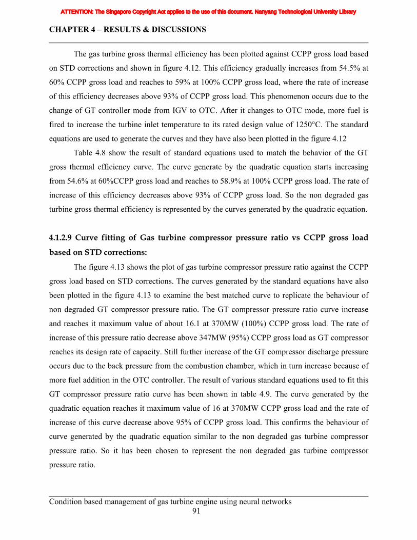
CHAPTER 4 – RESULTS & DISCUSSIONS ______________________________________________________________________________
The gas turbine gross thermal efficiency has been plotted against CCPP gross load based
on STD corrections and shown in figure 4.12. This efficiency gradually increases from 54.5% at
60% CCPP gross load and reaches to 59% at 100% CCPP gross load, where the rate of increase
of this efficiency decreases above 93% of CCPP gross load. This phenomenon occurs due to the
change of GT controller mode from IGV to OTC. After it changes to OTC mode, more fuel is
fired to increase the turbine inlet temperature to its rated design value of 1250°C. The standard
equations are used to generate the curves and they have also been plotted in the figure 4.12
Table 4.8 show the result of standard equations used to match the behavior of the GT
gross thermal efficiency curve. The curve generate by the quadratic equation starts increasing
from 54.6% at 60%CCPP gross load and reaches to 58.9% at 100% CCPP gross load. The rate of
increase of this efficiency decreases above 93% of CCPP gross load. So the non degraded gas
turbine gross thermal efficiency is represented by the curves generated by the quadratic equation.
4.1.2.9 Curve fitting of Gas turbine compressor pressure ratio vs CCPP gross load
based on STD corrections:
The figure 4.13 shows the plot of gas turbine compressor pressure ratio against the CCPP
gross load based on STD corrections. The curves generated by the standard equations have also
been plotted in the figure 4.13 to examine the best matched curve to replicate the behaviour of
non degraded GT compressor pressure ratio. The GT compressor pressure ratio curve increase
and reaches it maximum value of about 16.1 at 370MW (100%) CCPP gross load. The rate of
increase of this pressure ratio decrease above 347MW (95%) CCPP gross load as GT compressor
reaches its design rate of capacity. Still further increase of the GT compressor discharge pressure
occurs due to the back pressure from the combustion chamber, which in turn increase because of
more fuel addition in the OTC controller. The result of various standard equations used to fit this
GT compressor pressure ratio curve has been shown in table 4.9. The curve generated by the
quadratic equation reaches it maximum value of 16 at 370MW CCPP gross load and the rate of
increase of this curve decrease above 95% of CCPP gross load. This confirms the behaviour of
curve generated by the quadratic equation similar to the non degraded gas turbine compressor
pressure ratio. So it has been chosen to represent the non degraded gas turbine compressor
pressure ratio.
______________________________________________________________________________ Condition based management of gas turbine engine using neural networks 91
ATTENTION: The Singapore Copyright Act applies to the use of this document. Nanyang Technological University Library
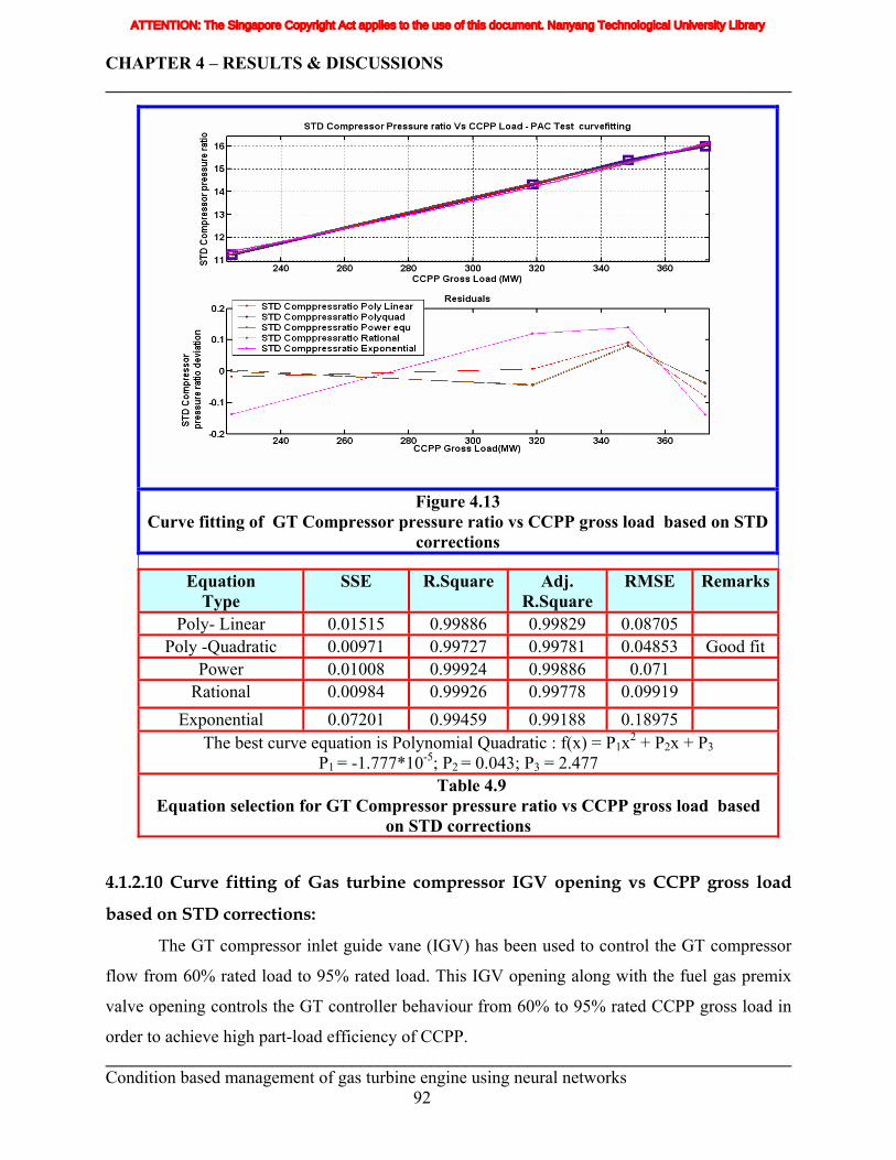
CHAPTER 4 – RESULTS & DISCUSSIONS ______________________________________________________________________________
Figure 4.13 Curve fitting of GT Compressor pressure ratio vs CCPP gross load based on STD
corrections
Equation Type
SSE R.Square Adj. R.Square
RMSE Remarks
Poly- Linear 0.01515 0.99886 0.99829 0.08705 Poly -Quadratic 0.00971 0.99727 0.99781 0.04853 Good fit
Power 0.01008 0.99924 0.99886 0.071 Rational 0.00984 0.99926 0.99778 0.09919
Exponential 0.07201 0.99459 0.99188 0.18975 The best curve equation is Polynomial Quadratic : f(x) = P1x2 + P2x + P3
P1 = -1.777*10-5; P2 = 0.043; P3 = 2.477 Table 4.9
Equation selection for GT Compressor pressure ratio vs CCPP gross load based on STD corrections
4.1.2.10 Curve fitting of Gas turbine compressor IGV opening vs CCPP gross load
based on STD corrections:
______________________________________________________________________________ Condition based management of gas turbine engine using neural networks 92
The GT compressor inlet guide vane (IGV) has been used to control the GT compressor
flow from 60% rated load to 95% rated load. This IGV opening along with the fuel gas premix
valve opening controls the GT controller behaviour from 60% to 95% rated CCPP gross load in
order to achieve high part-load efficiency of CCPP.
ATTENTION: The Singapore Copyright Act applies to the use of this document. Nanyang Technological University Library
CHAPTER 4 – RESULTS & DISCUSSIONS ______________________________________________________________________________
Figure 4.14 Curve fitting of GT Compressor IGV position vs CCPP gross load based on STD
corrections
Equation Type SSE R.Square Adj. R.Square
RMSE Remarks
Poly- Linear 72.41585 0.98895 0.98343 6.0173 Poly- Quadratic 7.8107 0.99881 0.99642 2.79476 Good fit
Guasian 9.87568 0.99849 0.99548 3.14256
Exponential 10.21845 0.99844
The best curve equation is Polynomial Quadratic: f(x) = P1x2 + P2x + P3 P1 = 0.001936; P2 = -0.4205; P3 = -2.987;
Table 4.10 Equation selection for GT Compressor IGV position vs CCPP gross load based on
STD corrections
The figure 4.14 shows the GT Compressor IGV position plot against the CCPP gross load
based on STD corrections and curves generated by the standard equation to examine their fitness
with GT Compressor IGV position curve. The IGV position increases with the increase of the
CCPP gross load based on STD correction. The rate of IGV position increase from 220MW
(60%) of CCPP gross load to 320MW (85%) of CCPP gross load is lesser when compared with
______________________________________________________________________________ Condition based management of gas turbine engine using neural networks 93
ATTENTION: The Singapore Copyright Act applies to the use of this document. Nanyang Technological University Library
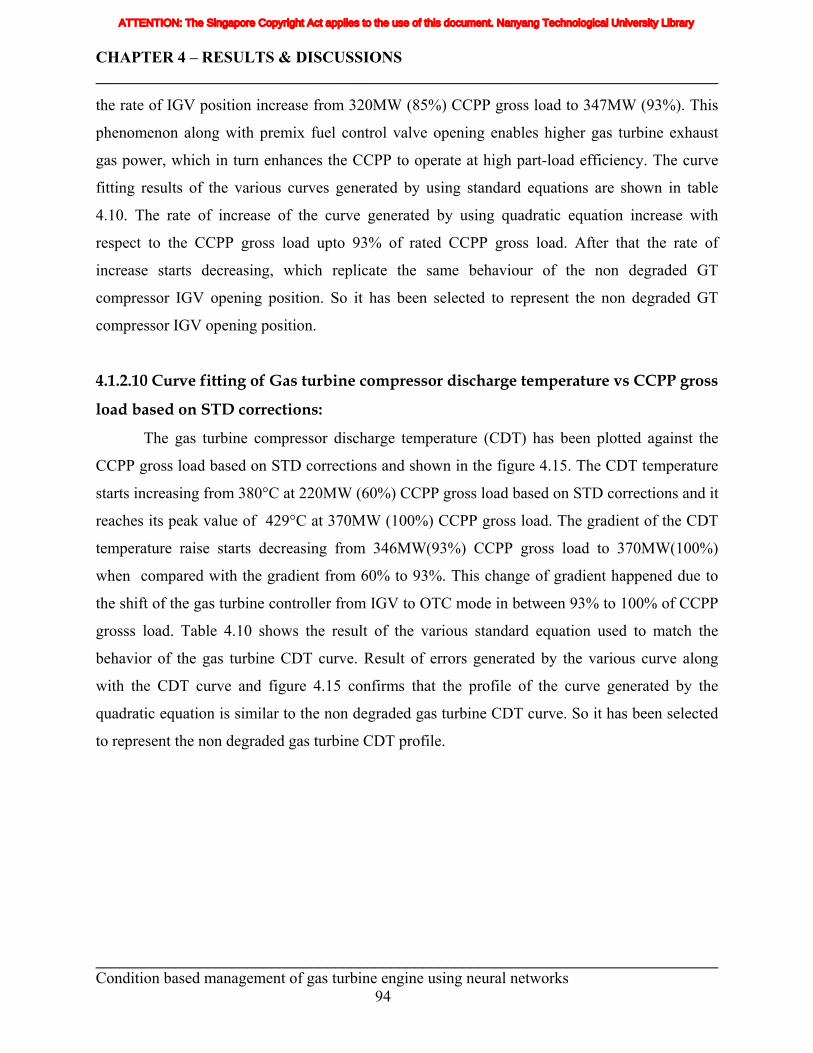
CHAPTER 4 – RESULTS & DISCUSSIONS ______________________________________________________________________________
the rate of IGV position increase from 320MW (85%) CCPP gross load to 347MW (93%). This
phenomenon along with premix fuel control valve opening enables higher gas turbine exhaust
gas power, which in turn enhances the CCPP to operate at high part-load efficiency. The curve
fitting results of the various curves generated by using standard equations are shown in table
4.10. The rate of increase of the curve generated by using quadratic equation increase with
respect to the CCPP gross load upto 93% of rated CCPP gross load. After that the rate of
increase starts decreasing, which replicate the same behaviour of the non degraded GT
compressor IGV opening position. So it has been selected to represent the non degraded GT
compressor IGV opening position.
4.1.2.10 Curve fitting of Gas turbine compressor discharge temperature vs CCPP gross
load based on STD corrections:
The gas turbine compressor discharge temperature (CDT) has been plotted against the
CCPP gross load based on STD corrections and shown in the figure 4.15. The CDT temperature
starts increasing from 380°C at 220MW (60%) CCPP gross load based on STD corrections and it
reaches its peak value of 429°C at 370MW (100%) CCPP gross load. The gradient of the CDT
temperature raise starts decreasing from 346MW(93%) CCPP gross load to 370MW(100%)
when compared with the gradient from 60% to 93%. This change of gradient happened due to
the shift of the gas turbine controller from IGV to OTC mode in between 93% to 100% of CCPP
grosss load. Table 4.10 shows the result of the various standard equation used to match the
behavior of the gas turbine CDT curve. Result of errors generated by the various curve along
with the CDT curve and figure 4.15 confirms that the profile of the curve generated by the
quadratic equation is similar to the non degraded gas turbine CDT curve. So it has been selected
to represent the non degraded gas turbine CDT profile.
______________________________________________________________________________ Condition based management of gas turbine engine using neural networks 94
ATTENTION: The Singapore Copyright Act applies to the use of this document. Nanyang Technological University Library
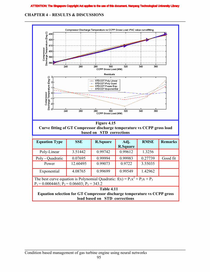
CHAPTER 4 – RESULTS & DISCUSSIONS ______________________________________________________________________________
Figure 4.15 Curve fitting of GT Compressor discharge temperature vs CCPP gross load
based on STD corrections
Equation Type SSE R.Square Adj. R.Square
RMSE Remarks
Poly-Linear 3.51442 0.99742 0.99612 1.3256 Poly - Quadratic 0.07695 0.99994 0.99983 0.27739 Good fit
Power 12.60495 0.99073 0.9722 3.55035
Exponential 4.08765 0.99699 0.99549 1.42962
The best curve equation is Polynomial Quadratic: f(x) = P1x2 + P2x + P3 P1 = 0.0004465; P2 = 0.06603; P3 = 343.2
Table 4.11 Equation selection for GT Compressor discharge temperature vs CCPP gross
load based on STD corrections ______________________________________________________________________________ Condition based management of gas turbine engine using neural networks 95
ATTENTION: The Singapore Copyright Act applies to the use of this document. Nanyang Technological University Library
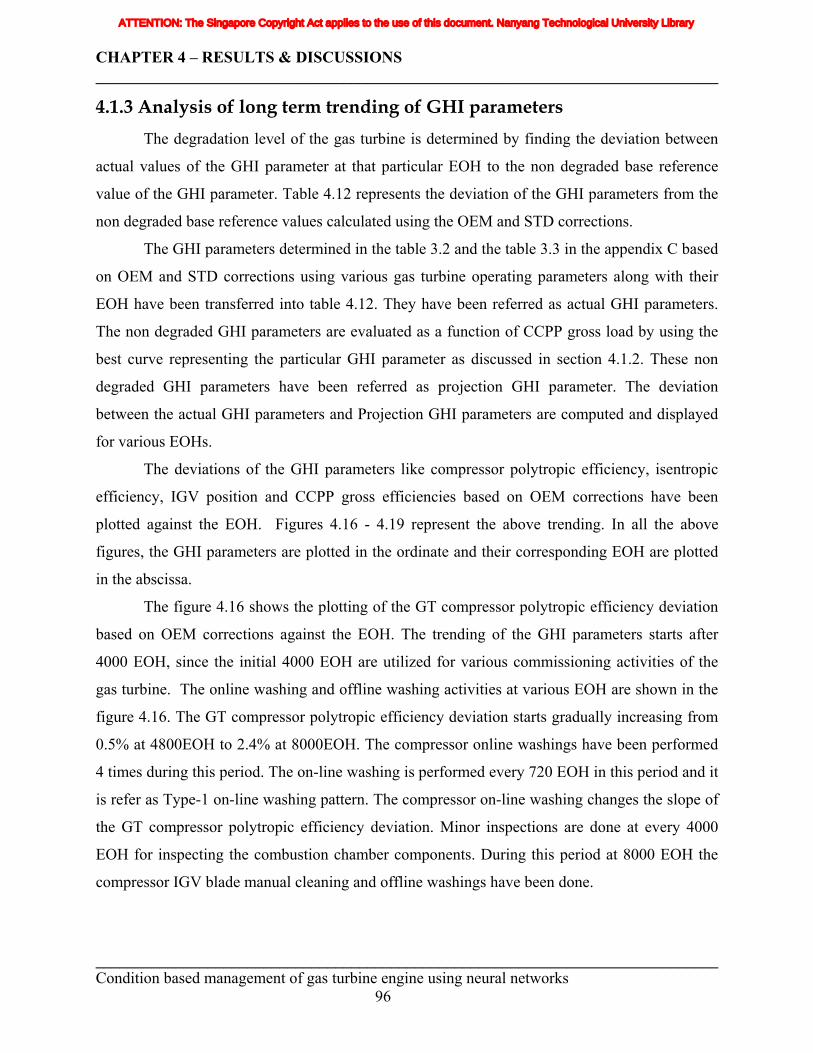
CHAPTER 4 – RESULTS & DISCUSSIONS ______________________________________________________________________________
______________________________________________________________________________ Condition based m
anagement of gas turbine engine using neural networks 96
4.1.3 Analysis of long term trending of GHI parameters The degradation level of the gas turbine is determined by finding the deviation between
actual values of the GHI parameter at that particular EOH to the non degraded base reference
value of the GHI parameter. Table 4.12 represents the deviation of the GHI parameters from the
non degraded base reference values calculated using the OEM and STD corrections.
The GHI parameters determined in the table 3.2 and the table 3.3 in the appendix C based
on OEM and STD corrections using various gas turbine operating parameters along with their
EOH have been transferred into table 4.12. They have been referred as actual GHI parameters.
The non degraded GHI parameters are evaluated as a function of CCPP gross load by using the
best curve representing the particular GHI parameter as discussed in section 4.1.2. These non
degraded GHI parameters have been referred as projection GHI parameter. The deviation
between the actual GHI parameters and Projection GHI parameters are computed and displayed
for various EOHs.
The deviations of the GHI parameters like compressor polytropic efficiency, isentropic
efficiency, IGV position and CCPP gross efficiencies based on OEM corrections have been
plotted against the EOH. Figures 4.16 - 4.19 represent the above trending. In all the above
figures, the GHI parameters are plotted in the ordinate and their corresponding EOH are plotted
in the abscissa.
The figure 4.16 shows the plotting of the GT compressor polytropic efficiency deviation
based on OEM corrections against the EOH. The trending of the GHI parameters starts after
4000 EOH, since the initial 4000 EOH are utilized for various commissioning activities of the
gas turbine. The online washing and offline washing activities at various EOH are shown in the
figure 4.16. The GT compressor polytropic efficiency deviation starts gradually increasing from
0.5% at 4800EOH to 2.4% at 8000EOH. The compressor online washings have been performed
4 times during this period. The on-line washing is performed every 720 EOH in this period and it
is refer as Type-1 on-line washing pattern. The compressor on-line washing changes the slope of
the GT compressor polytropic efficiency deviation. Minor inspections are done at every 4000
EOH for inspecting the combustion chamber components. During this period at 8000 EOH the
compressor IGV blade manual cleaning and offline washings have been done.
ATTENTION: The Singapore Copyright Act applies to the use of this document. Nanyang Technological University Library
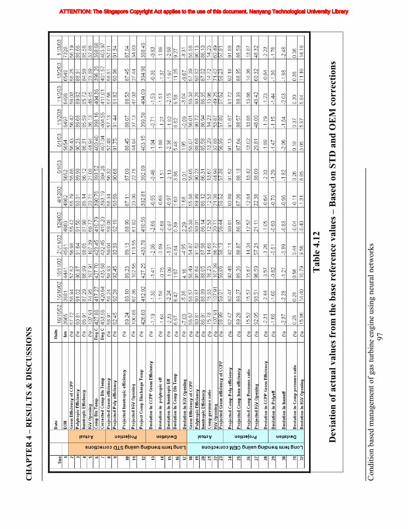
CH
APT
ER
4 –
RE
SUL
TS
& D
ISC
USS
ION
S __
____
____
____
____
____
____
____
____
____
____
____
____
____
____
____
____
____
____
____
Tab
le 4
.12
Dev
iatio
n of
act
ual v
alue
s fro
m th
e ba
se r
efer
ence
val
ues –
Bas
ed o
n ST
D a
nd O
EM
cor
rect
ions
____
____
____
____
____
____
____
____
____
____
____
____
____
____
____
____
____
____
____
__
Con
ditio
n ba
sed
man
agem
ent o
f gas
turb
ine
engi
ne u
sing
neu
ral n
etw
orks
97
ATTENTION: The Singapore Copyright Act applies to the use of this document. Nanyang Technological University Library
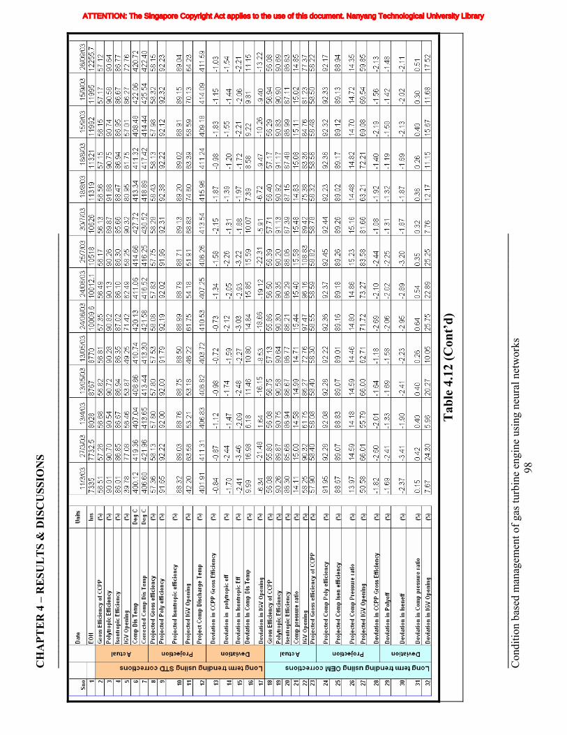
CH
APT
ER
4 –
RE
SUL
TS
& D
ISC
USS
ION
S __
____
____
____
____
____
____
____
____
____
____
____
____
____
____
____
____
____
____
____
Tab
le 4
.12
(Con
t’d)
____
____
____
____
____
____
____
____
____
____
____
____
____
____
____
____
____
____
____
__
Con
ditio
n ba
sed
man
agem
ent o
f gas
turb
ine
engi
ne u
sing
neu
ral n
etw
orks
98
ATTENTION: The Singapore Copyright Act applies to the use of this document. Nanyang Technological University Library
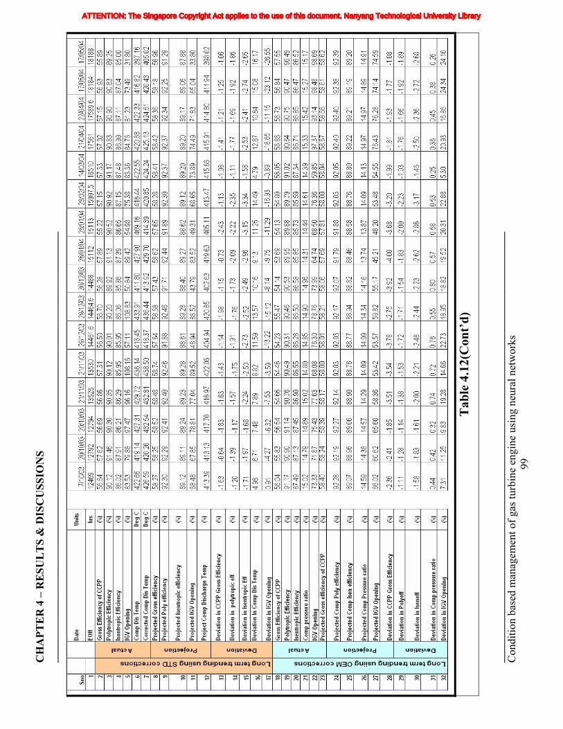
CH
APT
ER
4 –
RE
SUL
TS
& D
ISC
USS
ION
S __
____
____
____
____
____
____
____
____
____
____
____
____
____
____
____
____
____
____
____
____
____
____
____
____
____
____
____
____
____
____
____
____
____
____
____
____
____
____
__
Con
ditio
n ba
sed
m
Tab
le 4
.12(
Con
t’d)
anag
emen
t of g
as tu
rbin
e en
gine
usi
ng n
eura
l net
wor
ks
99
ATTENTION: The Singapore Copyright Act applies to the use of this document. Nanyang Technological University Library
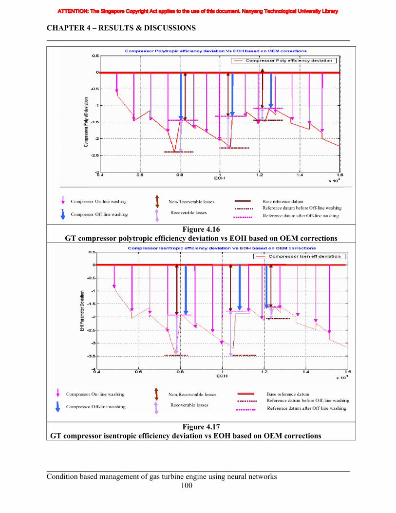
CHAPTER 4 – RESULTS & DISCUSSIONS ______________________________________________________________________________
Figure 4.16 GT compressor polytropic efficiency deviation vs EOH based on OEM corrections
Figure 4.17 GT compressor isentropic efficiency deviation vs EOH based on OEM corrections
______________________________________________________________________________ Condition based management of gas turbine engine using neural networks 100
ATTENTION: The Singapore Copyright Act applies to the use of this document. Nanyang Technological University Library
CHAPTER 4 – RESULTS & DISCUSSIONS ______________________________________________________________________________
After the IGV blade cleaning and compressor off-line washing activity the deviation of
the GT compressor polytropic efficiency decreases and reaches only about 1.4% and not to its
original value of 0%. This loss of 1.4% of GT compressor polytropic efficiency is due to non-
recoverable losses. The loss of 1.0% which is recovered by this IGV blade manual cleaning and
offline washing is considered as recoverable loss.
Three time compressor on-line washings have been done from 8000 EOH to 10518 EOH.
The on-line washing is performed every 584 EOH in this period and it is refer as Type-2 on-line
washing pattern. During this time period the GT compressor polytropic efficiency deviation
increases from 1.4% to 2.2%. Compressor IGV bade cleaning and offline washing activities have
been performed at 10626 EOH. The compressor polytropic efficiency deviation decreases to
1.4%. This confirms that loss of 1.4% of GT compressor polytropic efficiency deviation from its
original value of 0% as non recoverable losses and recovered efficiency of about 0.8% deviation
as recoverable losses.
The next compressor IGV blade cleaning and off-line washing activities have performed
during the minor inspection at 12500EOH. Two compressor on-line washings have been
performed between 11320 to 12260EOH with approximate time interval of 470 EOH. The GT
compressor polytropic efficiency deviation decreases to 1.2% after the 12500EOH. This
confirms the 1.2% is the non recoverable losses and 0.3% recovered by the manual blade
cleaning and offline washing as recoverable loss.
The GT compressor Polytropic efficiency deviation decreases to 2.3% at 16000EOH. The
compressor on-line washings have been done four times between 12500EOH and 16000EOH
with approximate time interval of 875 EOH. The recoverable loss of 0.9% deviation has been
occurred during the time period from 12500 EOH to 16000 EOH.
In order to have the easy reference of the number of on-line and time period between the
equivalent operating hours, following methods of classifications are done.
The on-line washing is classified into following types based time interval between two
successive on-line washings.
Type-1 refers that one on-line washing is performed for every 720 EOH.
Type-2 refers that one on-line washing is performed for every 584 EOH.
Type-3 refers that one on-line washing is performed for every 470 EOH.
______________________________________________________________________________ Condition based management of gas turbine engine using neural networks 101
ATTENTION: The Singapore Copyright Act applies to the use of this document. Nanyang Technological University Library
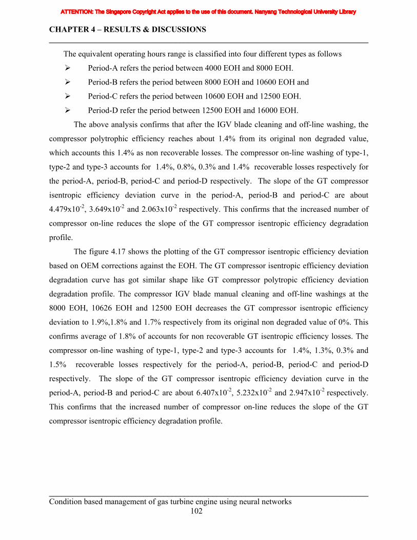
CHAPTER 4 – RESULTS & DISCUSSIONS ______________________________________________________________________________
The equivalent operating hours range is classified into four different types as follows
Period-A refers the period between 4000 EOH and 8000 EOH.
Period-B refers the period between 8000 EOH and 10600 EOH and
Period-C refers the period between 10600 EOH and 12500 EOH.
Period-D refer the period between 12500 EOH and 16000 EOH.
The above analysis confirms that after the IGV blade cleaning and off-line washing, the
compressor polytrophic efficiency reaches about 1.4% from its original non degraded value,
which accounts this 1.4% as non recoverable losses. The compressor on-line washing of type-1,
type-2 and type-3 accounts for 1.4%, 0.8%, 0.3% and 1.4% recoverable losses respectively for
the period-A, period-B, period-C and period-D respectively. The slope of the GT compressor
isentropic efficiency deviation curve in the period-A, period-B and period-C are about
4.479x10⁻², 3.649x10⁻² and 2.063x10⁻² respectively. This confirms that the increased number of
compressor on-line reduces the slope of the GT compressor isentropic efficiency degradation
profile.
The figure 4.17 shows the plotting of the GT compressor isentropic efficiency deviation
based on OEM corrections against the EOH. The GT compressor isentropic efficiency deviation
degradation curve has got similar shape like GT compressor polytropic efficiency deviation
degradation profile. The compressor IGV blade manual cleaning and off-line washings at the
8000 EOH, 10626 EOH and 12500 EOH decreases the GT compressor isentropic efficiency
deviation to 1.9%,1.8% and 1.7% respectively from its original non degraded value of 0%. This
confirms average of 1.8% of accounts for non recoverable GT isentropic efficiency losses. The
compressor on-line washing of type-1, type-2 and type-3 accounts for 1.4%, 1.3%, 0.3% and
1.5% recoverable losses respectively for the period-A, period-B, period-C and period-D
respectively. The slope of the GT compressor isentropic efficiency deviation curve in the
period-A, period-B and period-C are about 6.407x10⁻², 5.232x10⁻² and 2.947x10⁻² respectively.
This confirms that the increased number of compressor on-line reduces the slope of the GT
compressor isentropic efficiency degradation profile.
______________________________________________________________________________ Condition based management of gas turbine engine using neural networks 102
ATTENTION: The Singapore Copyright Act applies to the use of this document. Nanyang Technological University Library
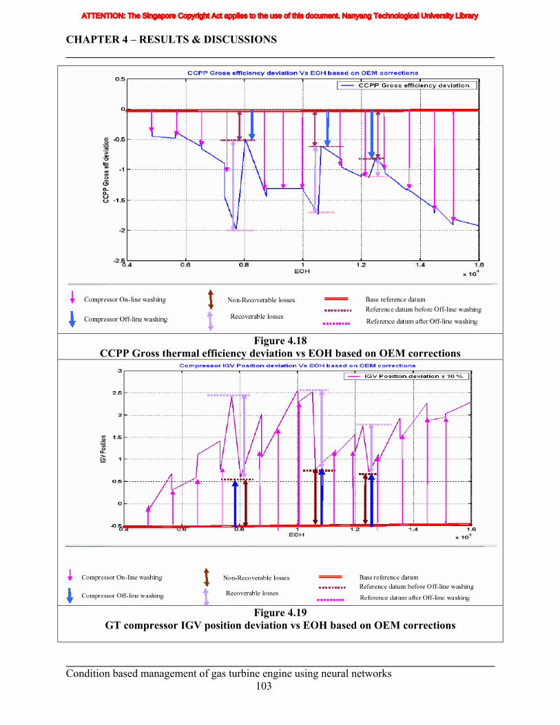
CHAPTER 4 – RESULTS & DISCUSSIONS ______________________________________________________________________________
Figure 4.18
CCPP Gross thermal efficiency deviation vs EOH based on OEM corrections
Figure 4.19
GT compressor IGV position deviation vs EOH based on OEM corrections
______________________________________________________________________________ Condition based management of gas turbine engine using neural networks 103
ATTENTION: The Singapore Copyright Act applies to the use of this document. Nanyang Technological University Library
CHAPTER 4 – RESULTS & DISCUSSIONS ______________________________________________________________________________
The CCPP gross thermal efficiency deviation from the non degraded value for various
EOH has been plotted in the figure 4.18. The analysis shows that the compressor off-line and
IGV blade manual cleaning activities reduces the CCPP gross thermal efficiency deviation to
0.5%, 0.7% and 0.8%. These are the non recoverable CCPP gross thermal efficiency at
8000 EOH, 10800 EOH and 12500 EOH respectively. The recoverable losses of about 1.5%,
1.0%, 0.4%, for the period-A, period-B, period-C are achieved with on-line washing of type-1,
type-2 and type-3 respectively. The slope of the gross thermal efficiency deviation curve in the
period-A, period-B and period-C are about 5.0 x10⁻⁴, 3.846 x10⁻⁴ and 3.421x10⁻⁴ respectively.
This shows that the increased number of on-line washing reduces the slope of the GHI parameter
deviation profile.
The gas turbine under study is always used to run at below 90% of its rated capacity due
to spinning reserve set by the power grid. The airflow rate of the gas turbine is controlled by the
IGV position from the 60% rated load to around 95% rated load. (Refer the gas turbine controller
of CCPP, figure 2.22). Under base load conditions the effect of fouling on the airflow rate and
pressure ratio can be easily determined by comparing the actual output with the base reference
value. But during part load operations the effect of fouling on the compressor airflow rate and
pressure ratio is difficult to find out, since the IGV opens more and tries to compensate the
degraded airflow rate and pressure ratio. So the effect of the airflow rate and pressure ratio can
be determined by plotting the IGV position against the CCPP gross load. The fouling of the
compressor will lead for more opening of the IGV.
The figure 4.19 shows the plot of GT compressor IGV position deviation from the non
degraded IGV compressor position for various EOH. The IGV opening deviation gradually
increases along with EOH during normal operation and reduces after the compressor IGV blade
cleaning and off-line washings. The compressor IGV blade cleaning and off-line washing
decreases the IGV opening position deviation from 2.5% to 0.5% of their non degraded value,
whereas the compressor on-line washing decrease the slope of the increase of IGV opening
deviation curve.
Figures 4.20 – 4.24 shows the plot of GT compressor polytropic efficiency deviation,
isentropic efficiency deviation, CCPP gross efficiency deviation, compressor IGV position
______________________________________________________________________________ Condition based management of gas turbine engine using neural networks 104
ATTENTION: The Singapore Copyright Act applies to the use of this document. Nanyang Technological University Library
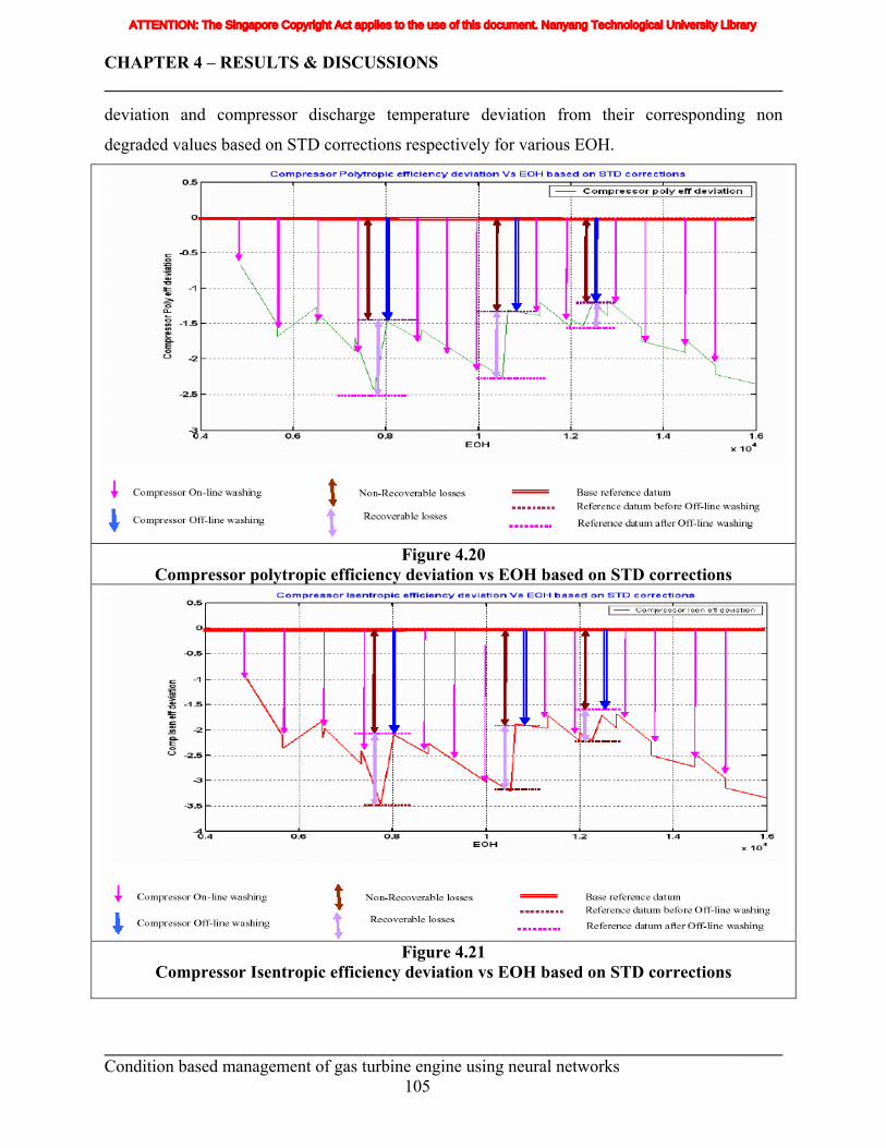
CHAPTER 4 – RESULTS & DISCUSSIONS ______________________________________________________________________________
deviation and compressor discharge temperature deviation from their corresponding non
degraded values based on STD corrections respectively for various EOH.
Figure 4.20
Compressor polytropic efficiency deviation vs EOH based on STD corrections
Figure 4.21
Compressor Isentropic efficiency deviation vs EOH based on STD corrections ______________________________________________________________________________ Condition based management of gas turbine engine using neural networks 105
ATTENTION: The Singapore Copyright Act applies to the use of this document. Nanyang Technological University Library
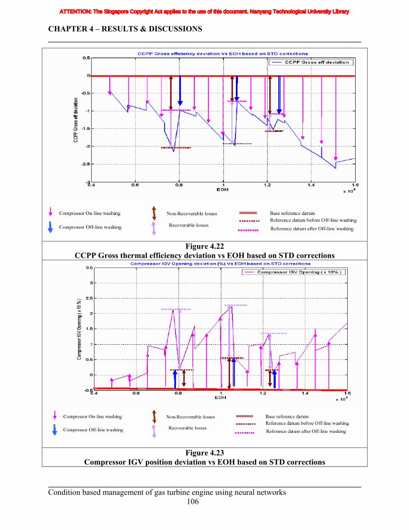
CHAPTER 4 – RESULTS & DISCUSSIONS ______________________________________________________________________________
Figure 4.22
CCPP Gross thermal efficiency deviation vs EOH based on STD corrections
Figure 4.23 Compressor IGV position deviation vs EOH based on STD corrections
______________________________________________________________________________ Condition based management of gas turbine engine using neural networks 106
ATTENTION: The Singapore Copyright Act applies to the use of this document. Nanyang Technological University Library
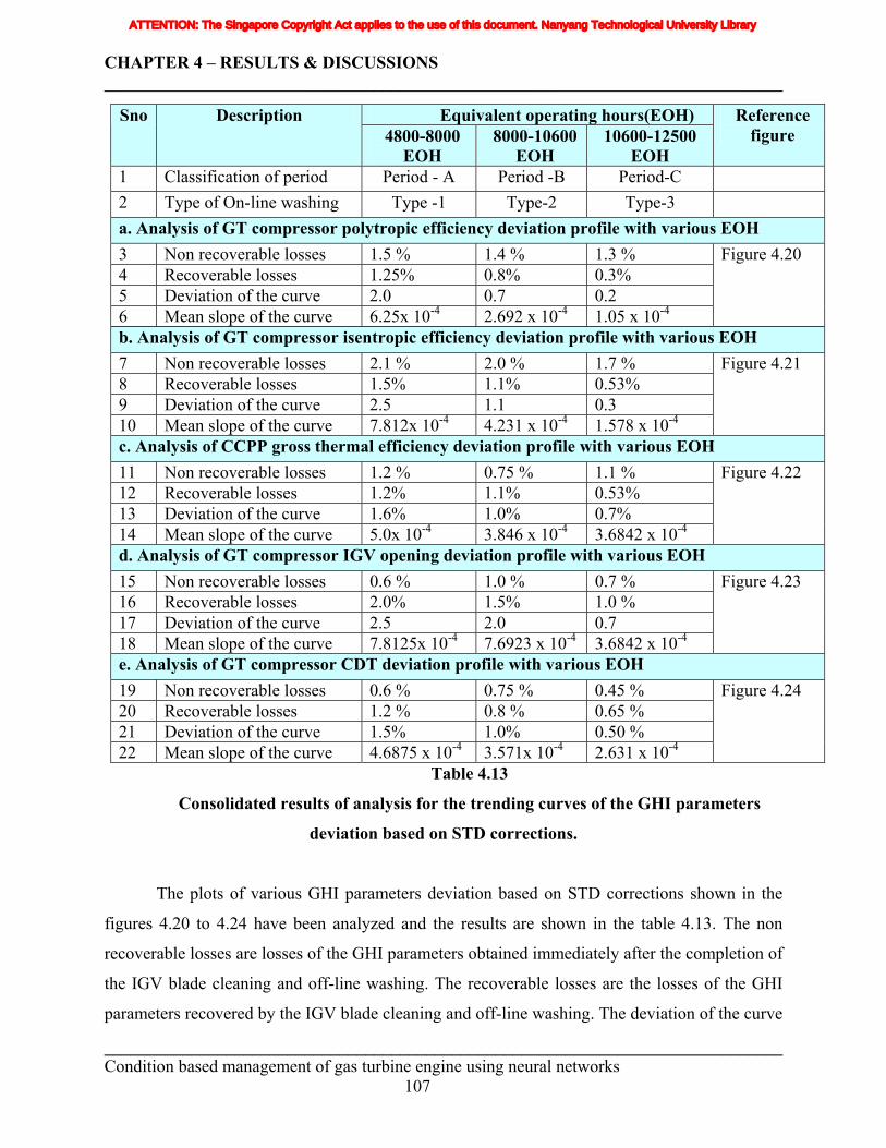
CHAPTER 4 – RESULTS & DISCUSSIONS ______________________________________________________________________________
Equivalent operating hours(EOH) Sno Description 4800-8000
EOH 8000-10600
EOH 10600-12500
EOH
Reference figure
1 Classification of period Period - A Period -B Period-C 2 Type of On-line washing Type -1 Type-2 Type-3 a. Analysis of GT compressor polytropic efficiency deviation profile with various EOH 3 Non recoverable losses 1.5 % 1.4 % 1.3 % 4 Recoverable losses 1.25% 0.8% 0.3% 5 Deviation of the curve 2.0 0.7 0.2 6 Mean slope of the curve 6.25x 10⁻⁴ 2.692 x 10⁻⁴ 1.05 x 10⁻⁴
Figure 4.20
b. Analysis of GT compressor isentropic efficiency deviation profile with various EOH 7 Non recoverable losses 2.1 % 2.0 % 1.7 % 8 Recoverable losses 1.5% 1.1% 0.53% 9 Deviation of the curve 2.5 1.1 0.3 10 Mean slope of the curve 7.812x 10⁻⁴ 4.231 x 10⁻⁴ 1.578 x 10⁻⁴
Figure 4.21
c. Analysis of CCPP gross thermal efficiency deviation profile with various EOH 11 Non recoverable losses 1.2 % 0.75 % 1.1 % 12 Recoverable losses 1.2% 1.1% 0.53% 13 Deviation of the curve 1.6% 1.0% 0.7% 14 Mean slope of the curve 5.0x 10⁻⁴ 3.846 x 10⁻⁴ 3.6842 x 10⁻⁴
Figure 4.22
d. Analysis of GT compressor IGV opening deviation profile with various EOH 15 Non recoverable losses 0.6 % 1.0 % 0.7 % 16 Recoverable losses 2.0% 1.5% 1.0 % 17 Deviation of the curve 2.5 2.0 0.7 18 Mean slope of the curve 7.8125x 10⁻⁴ 7.6923 x 10⁻⁴ 3.6842 x 10⁻⁴
Figure 4.23
e. Analysis of GT compressor CDT deviation profile with various EOH 19 Non recoverable losses 0.6 % 0.75 % 0.45 % 20 Recoverable losses 1.2 % 0.8 % 0.65 % 21 Deviation of the curve 1.5% 1.0% 0.50 % 22 Mean slope of the curve 4.6875 x 10⁻⁴ 3.571x 10⁻⁴ 2.631 x 10⁻⁴
Figure 4.24
Table 4.13
Consolidated results of analysis for the trending curves of the GHI parameters
deviation based on STD corrections.
The plots of various GHI parameters deviation based on STD corrections shown in the
figures 4.20 to 4.24 have been analyzed and the results are shown in the table 4.13. The non
recoverable losses are losses of the GHI parameters obtained immediately after the completion of
the IGV blade cleaning and off-line washing. The recoverable losses are the losses of the GHI
parameters recovered by the IGV blade cleaning and off-line washing. The deviation of the curve
______________________________________________________________________________ Condition based management of gas turbine engine using neural networks 107
ATTENTION: The Singapore Copyright Act applies to the use of this document. Nanyang Technological University Library
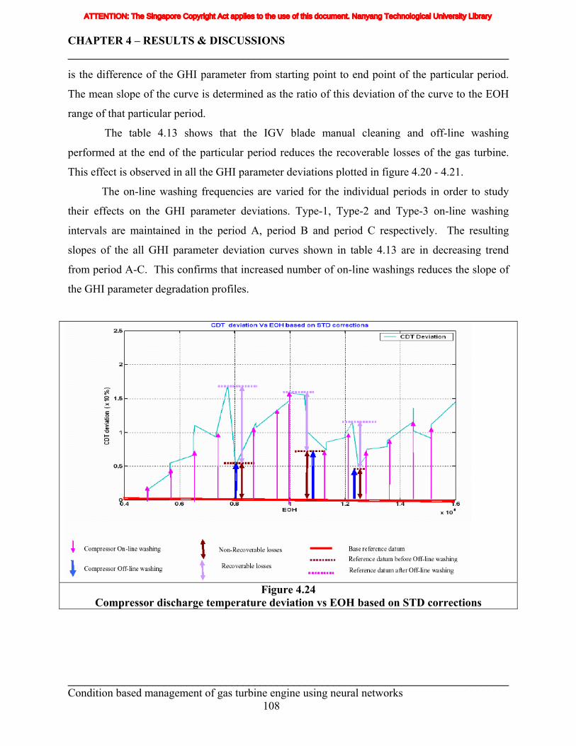
CHAPTER 4 – RESULTS & DISCUSSIONS ______________________________________________________________________________
is the difference of the GHI parameter from starting point to end point of the particular period.
The mean slope of the curve is determined as the ratio of this deviation of the curve to the EOH
range of that particular period.
The table 4.13 shows that the IGV blade manual cleaning and off-line washing
performed at the end of the particular period reduces the recoverable losses of the gas turbine.
This effect is observed in all the GHI parameter deviations plotted in figure 4.20 - 4.21.
The on-line washing frequencies are varied for the individual periods in order to study
their effects on the GHI parameter deviations. Type-1, Type-2 and Type-3 on-line washing
intervals are maintained in the period A, period B and period C respectively. The resulting
slopes of the all GHI parameter deviation curves shown in table 4.13 are in decreasing trend
from period A-C. This confirms that increased number of on-line washings reduces the slope of
the GHI parameter degradation profiles.
Figure 4.24
Compressor discharge temperature deviation vs EOH based on STD corrections
______________________________________________________________________________ Condition based management of gas turbine engine using neural networks 108
ATTENTION: The Singapore Copyright Act applies to the use of this document. Nanyang Technological University Library
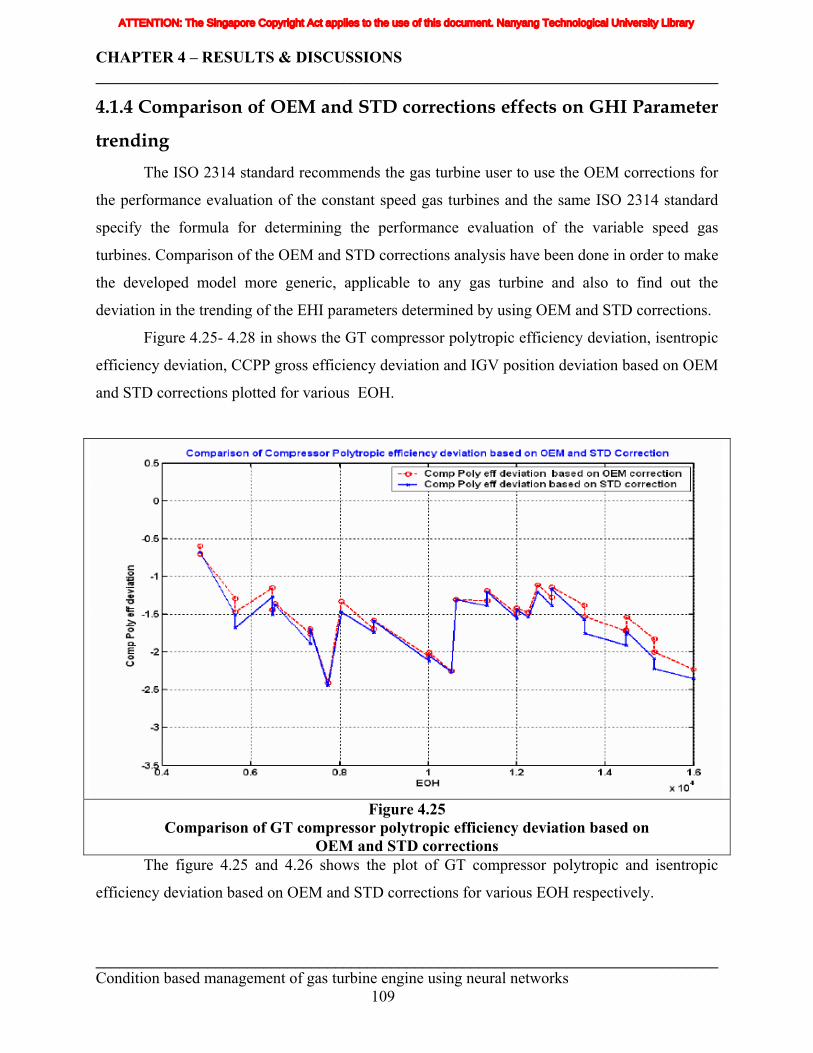
CHAPTER 4 – RESULTS & DISCUSSIONS ______________________________________________________________________________
4.1.4 Comparison of OEM and STD corrections effects on GHI Parameter
trending The ISO 2314 standard recommends the gas turbine user to use the OEM corrections for
the performance evaluation of the constant speed gas turbines and the same ISO 2314 standard
specify the formula for determining the performance evaluation of the variable speed gas
turbines. Comparison of the OEM and STD corrections analysis have been done in order to make
the developed model more generic, applicable to any gas turbine and also to find out the
deviation in the trending of the EHI parameters determined by using OEM and STD corrections.
Figure 4.25- 4.28 in shows the GT compressor polytropic efficiency deviation, isentropic
efficiency deviation, CCPP gross efficiency deviation and IGV position deviation based on OEM
and STD corrections plotted for various EOH.
Figure 4.25
Comparison of GT compressor polytropic efficiency deviation based on OEM and STD corrections
The figure 4.25 and 4.26 shows the plot of GT compressor polytropic and isentropic
efficiency deviation based on OEM and STD corrections for various EOH respectively.
______________________________________________________________________________ Condition based management of gas turbine engine using neural networks 109
ATTENTION: The Singapore Copyright Act applies to the use of this document. Nanyang Technological University Library
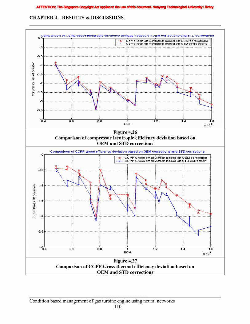
CHAPTER 4 – RESULTS & DISCUSSIONS ______________________________________________________________________________
Figure 4.26
Comparison of compressor Isentropic efficiency deviation based on OEM and STD corrections
Figure 4.27
Comparison of CCPP Gross thermal efficiency deviation based on OEM and STD corrections
______________________________________________________________________________ Condition based management of gas turbine engine using neural networks 110
ATTENTION: The Singapore Copyright Act applies to the use of this document. Nanyang Technological University Library
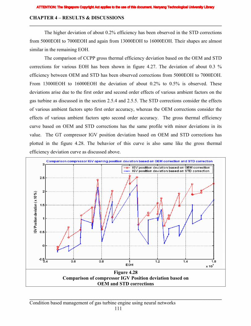
CHAPTER 4 – RESULTS & DISCUSSIONS ______________________________________________________________________________
The higher deviation of about 0.2% efficiency has been observed in the STD corrections
from 5000EOH to 7000EOH and again from 13000EOH to 16000EOH. Their shapes are almost
similar in the remaining EOH.
The comparison of CCPP gross thermal efficiency deviation based on the OEM and STD
corrections for various EOH has been shown in figure 4.27. The deviation of about 0.3 %
efficiency between OEM and STD has been observed corrections from 5000EOH to 7000EOH.
From 13000EOH to 16000EOH the deviation of about 0.2% to 0.5% is observed. These
deviations arise due to the first order and second order effects of various ambient factors on the
gas turbine as discussed in the section 2.5.4 and 2.5.5. The STD corrections consider the effects
of various ambient factors upto first order accuracy, whereas the OEM corrections consider the
effects of various ambient factors upto second order accuracy. The gross thermal efficiency
curve based on OEM and STD corrections has the same profile with minor deviations in its
value. The GT compressor IGV position deviation based on OEM and STD corrections has
plotted in the figure 4.28. The behavior of this curve is also same like the gross thermal
efficiency deviation curve as discussed above.
Figure 4.28
Comparison of compressor IGV Position deviation based on OEM and STD corrections
______________________________________________________________________________ Condition based management of gas turbine engine using neural networks 111
ATTENTION: The Singapore Copyright Act applies to the use of this document. Nanyang Technological University Library
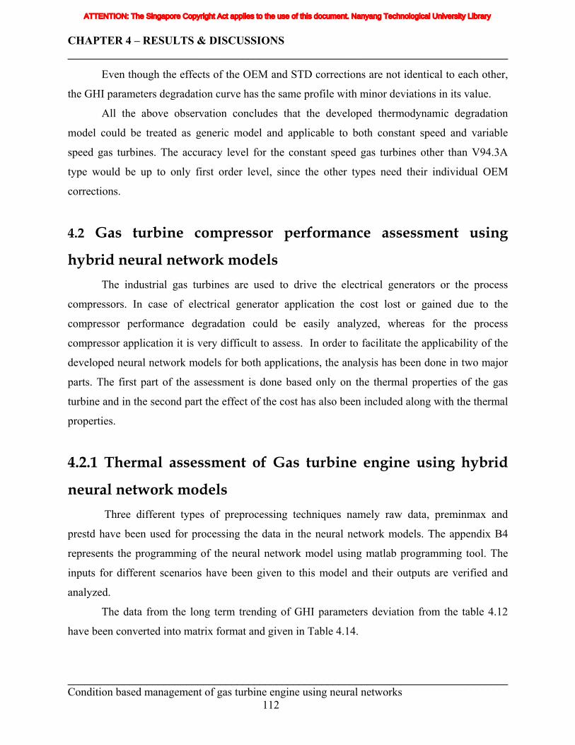
CHAPTER 4 – RESULTS & DISCUSSIONS ______________________________________________________________________________
Even though the effects of the OEM and STD corrections are not identical to each other,
the GHI parameters degradation curve has the same profile with minor deviations in its value.
All the above observation concludes that the developed thermodynamic degradation
model could be treated as generic model and applicable to both constant speed and variable
speed gas turbines. The accuracy level for the constant speed gas turbines other than V94.3A
type would be up to only first order level, since the other types need their individual OEM
corrections.
4.2 Gas turbine compressor performance assessment using
hybrid neural network models The industrial gas turbines are used to drive the electrical generators or the process
compressors. In case of electrical generator application the cost lost or gained due to the
compressor performance degradation could be easily analyzed, whereas for the process
compressor application it is very difficult to assess. In order to facilitate the applicability of the
developed neural network models for both applications, the analysis has been done in two major
parts. The first part of the assessment is done based only on the thermal properties of the gas
turbine and in the second part the effect of the cost has also been included along with the thermal
properties.
4.2.1 Thermal assessment of Gas turbine engine using hybrid
neural network models Three different types of preprocessing techniques namely raw data, preminmax and
prestd have been used for processing the data in the neural network models. The appendix B4
represents the programming of the neural network model using matlab programming tool. The
inputs for different scenarios have been given to this model and their outputs are verified and
analyzed.
The data from the long term trending of GHI parameters deviation from the table 4.12
have been converted into matrix format and given in Table 4.14.
______________________________________________________________________________ Condition based management of gas turbine engine using neural networks 112
ATTENTION: The Singapore Copyright Act applies to the use of this document. Nanyang Technological University Library
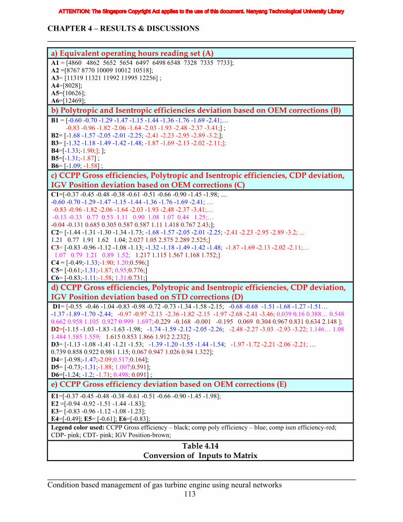
CHAPTER 4 – RESULTS & DISCUSSIONS ______________________________________________________________________________
a) Equivalent operating hours reading set (A) A1 = [4860 4862 5652 5654 6497 6498 6548 7328 7335 7733]; A2 =[8767 8770 10009 10012 10518]; A3= [11319 11321 11992 11995 12256] ; A4=[8028]; A5=[10626]; A6=[12469]; b) Polytropic and Isentropic efficiencies deviation based on OEM corrections (B) B1 = [-0.60 -0.70 -1.29 -1.47 -1.15 -1.44 -1.36 -1.76 -1.69 -2.41;… -0.83 -0.96 -1.82 -2.06 -1.64 -2.03 -1.93 -2.48 -2.37 -3.41;] ; B2= [-1.68 -1.57 -2.05 -2.01 -2.25; -2.41 -2.23 -2.95 -2.89 -3.2;]; B3= [-1.32 -1.18 -1.49 -1.42 -1.48; -1.87 -1.69 -2.13 -2.02 -2.11;]; B4=[-1.33;-1.90;]; ]; B5=[-1.31;-1.87] ; B6= [-1.09; -1.58] ; c) CCPP Gross efficiencies, Polytropic and Isentropic efficiencies, CDP deviation, IGV Position deviation based on OEM corrections (C) C1=[-0.37 -0.45 -0.48 -0.38 -0.61 -0.51 -0.66 -0.90 -1.45 -1.98; .... -0.60 -0.70 -1.29 -1.47 -1.15 -1.44 -1.36 -1.76 -1.69 -2.41; … -0.83 -0.96 -1.82 -2.06 -1.64 -2.03 -1.93 -2.48 -2.37 -3.41;… -0.13 -0.33 0.77 0.53 1.11 0.90 1.08 1.07 0.44 1.25;… -0.04 -0.131 0.685 0.305 0.587 0.587 1.11 1.418 0.767 2.43;]; C2= [-1.44 -1.31 -1.30 -1.34 -1.73; -1.68 -1.57 -2.05 -2.01 -2.25; -2.41 -2.23 -2.95 -2.89 -3.2; ... 1.21 0.77 1.91 1.62 1.04; 2.027 1.05 2.575 2.289 2.525;] C3= [-0.83 -0.96 -1.12 -1.08 -1.13; -1.32 -1.18 -1.49 -1.42 -1.48; -1.87 -1.69 -2.13 -2.02 -2.11;… 1.07 0.79 1.21 0.89 1.52; 1.217 1.115 1.567 1.168 1.752;] C4 = [-0.49;-1.33;-1.90; 1.20;0.596;] C5= [-0.61;-1.31;-1.87; 0.95;0.776;] C6= [-0.83;-1.11;-1.58; 1.31;0.731;] d) CCPP Gross efficiencies, Polytropic and Isentropic efficiencies, CDP deviation, IGV Position deviation based on STD corrections (D) D1= [-0.55 -0.46 -1.04 -0.83 -0.98 -0.72 -0.73 -1.34 -1.58 -2.15; -0.68 -0.68 -1.51 -1.68 -1.27 -1.51… -1.37 -1.89 -1.70 -2.44; -0.97 -0.97 -2.13 -2.36 -1.82 -2.15 -1.97 -2.68 -2.41 -3.46; 0.039 0.16 0.388… 0.548 0.662 0.958 1.105 0.927 0.999 1.697;-0.229 -0.168 -0.001 -0.195 0.069 0.304 0.967 0.831 0.634 2.148 ]; D2=[-1.15 -1.03 -1.83 -1.63 -1.98; -1.74 -1.59 -2.12 -2.05 -2.26; -2.48 -2.27 -3.03 -2.93 -3.22; 1.146… 1.08 1.484 1.585 1.559; 1.615 0.853 1.866 1.912 2.232]; D3= [-1.13 -1.08 -1.41 -1.21 -1.53; -1.39 -1.20 -1.55 -1.44 -1.54; -1.97 -1.72 -2.21 -2.06 -2.21; … 0.739 0.858 0.922 0.981 1.15; 0.067 0.947 1.026 0.94 1.322]; D4= [-0.98;-1.47;-2.09;0.517;0.164]; D5= [-0.73;-1.31;-1.88; 1.007;0.591]; D6=[-1.24; -1.2; -1.71; 0.498; 0.091] ; e) CCPP Gross efficiency deviation based on OEM corrections (E) E1=[-0.37 -0.45 -0.48 -0.38 -0.61 -0.51 -0.66 -0.90 -1.45 -1.98]; E2 =[-0.94 -0.92 -1.51 -1.44 -1.83]; E3= [-0.83 -0.96 -1.12 -1.08 -1.23]; E4=[-0.49]; E5= [-0.61]; E6=[-0.83]; Legend color used: CCPP Gross efficiency – black; comp poly efficiency – blue; comp isen efficiency-red; CDP- pink; CDT- pink; IGV Position-brown;
Table 4.14 Conversion of Inputs to Matrix
______________________________________________________________________________ Condition based management of gas turbine engine using neural networks 113
ATTENTION: The Singapore Copyright Act applies to the use of this document. Nanyang Technological University Library
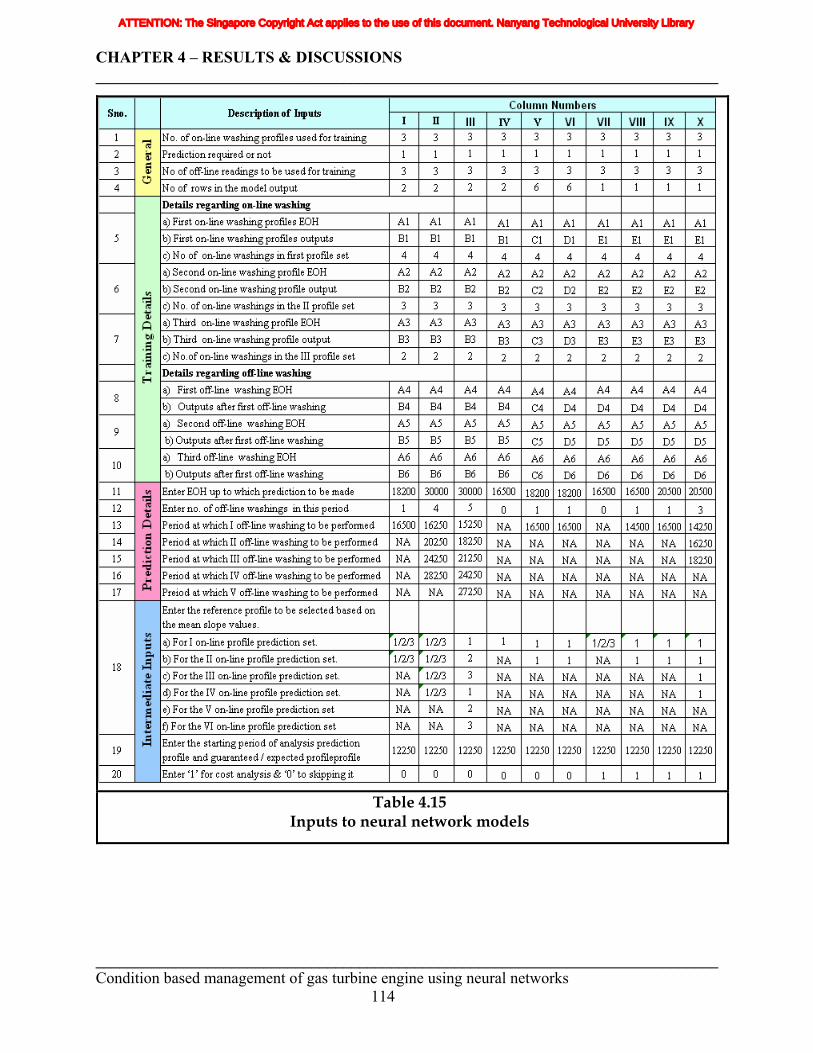
CHAPTER 4 – RESULTS & DISCUSSIONS ______________________________________________________________________________
Table 4.15 Inputs to neural network models
______________________________________________________________________________ Condition based management of gas turbine engine using neural networks 114
ATTENTION: The Singapore Copyright Act applies to the use of this document. Nanyang Technological University Library
CHAPTER 4 – RESULTS & DISCUSSIONS ______________________________________________________________________________
In the table 4.14, the value of the GHI parameters deviation and equivalent operating hours are
represented by alphanumerical symbols.
The alphabet “A” represent the matrix consist of equivalent operating hours values.
The alphabet “B” represent the matrix consist of polytropic and isentropic efficiency
deviation based on OEM corrections. In this matrix first row represent the polytropic
efficiency deviations and second row represent isentropic efficiency deviations.
The alphabet “C” represent the matrix consist of CCPP Gross, polytropic and isentropic
efficiencies, CDP deviation, IGV position deviation based on OEM corrections. The rows
of the matrix are arranged from one to five in the same sequence as mentioned as above.
The alphabet “D” represent the matrix consist of CCPP Gross, polytropic and isentropic
efficiencies, CDP deviation, IGV position deviation based on STD corrections. The rows
of the matrix are arranged from one to five in the same sequence as mentioned as above.
The alphabet “E” represent the matrix consist of CCPP gross efficiency deviation based
on OEM corrections.
The numerical values are used to classify the time interval from where the above readings
are taken. The numerical values 1, 2 and 3 represents the period-A (4800EOH to 8000EOH),
period-B (8000EOH to 10600EOH) and period-C (10600EOH to 12500EOH) respectively.
The numerical values 4, 5 and 6 represent the EOH when the first, second and third off-line
compressor washings are performed.
eg. The alphanumerical symbol “E3” represent the matrix consist of CCPP gross efficiency
deviation values from the period-C.
These alphanumerical symbols have been used to represent the input data to the various neural
network models in Table 4.15.
4.2.1.1 Analysis of the on-line washing of type 1 with off-line washing at 16500 EOH
The main objective of this analysis is to verify the developed hybrid neural network
model. The GHI parameters deviation and details about the compressor washings from 4800
EOH to 12600EOH are known and they are used for training the developed hybrid neural
network model. Even though the GHI parameters deviation and details about the compressor
washings from 12600EOH to 16800EOH are known, they have been hidden from the model. The
model outputs are generated for 12600EOH to 16800EOH for the same condition as mentioned
______________________________________________________________________________ Condition based management of gas turbine engine using neural networks 115
ATTENTION: The Singapore Copyright Act applies to the use of this document. Nanyang Technological University Library
CHAPTER 4 – RESULTS & DISCUSSIONS ______________________________________________________________________________
above. Then these outputs are compared with hidden real outputs of the gas turbine as a part
verification of the developed hybrid model.
The compressor polytropic efficiency and isentropic efficiency deviations based on OEM
corrections are analyzed by using this model. The data from the first column of the table 4.15
have been applied to the hybrid neural network model based on the Prestd technique as shown in
appendix B4.
The analysis 1.1.1 explains the internal outputs of this model. The internal outputs are
explained in steps.
Step 1
In the first step, the individual networks are developed for off-line washing
profile, first on-line washing profile, second on-line washing profile and third on-line
washing profile respectively. The individual trained networks performance (MSE) and
their residuals with the training values are shown in this step.
Step 2
The mean slopes of the three on-line washing profiles are determined in the
second step. These mean slopes indicate the rate of degradation of the EHI parameter
and they are directly proportional to the engine degradation rate. The third on-line
washing profile is having the lower mean slope value when compared with other two
profiles.
Step 3
The average time interval between the on-line washing profiles has been
determined in this step. The third on-line washing profile has the lower most time interval
between the on-line washings.
Step 4
In this step the user is allowed to select the profile which is to be used as
reference for the prediction part. The frequency of on-line washing interval maintained
from 12500 to 18500 is almost equivalent to the type-1 washing interval. So the first on-
line washing profile is selected as reference profile for the first and second prediction set.
This selection has been done in order to verify the model prediction part with the actual
machine behavior.
______________________________________________________________________________ Condition based management of gas turbine engine using neural networks 116
ATTENTION: The Singapore Copyright Act applies to the use of this document. Nanyang Technological University Library
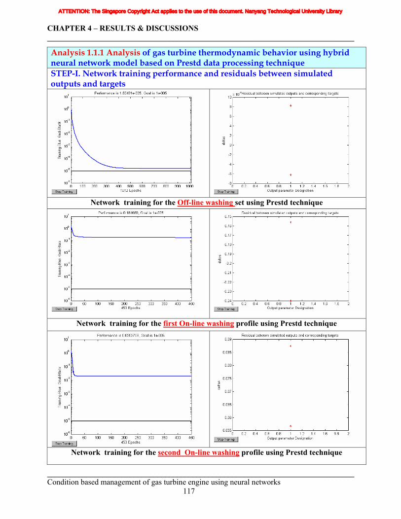
CHAPTER 4 – RESULTS & DISCUSSIONS ______________________________________________________________________________
Analysis 1.1.1 Analysis of gas turbine thermodynamic behavior using hybrid neural network model based on Prestd data processing technique STEP-I. Network training performance and residuals between simulated outputs and targets
Network training for the Off-line washing set using Prestd technique
Network training for the first On-line washing profile using Prestd technique
Network training for the second On-line washing profile using Prestd technique
______________________________________________________________________________ Condition based management of gas turbine engine using neural networks 117
ATTENTION: The Singapore Copyright Act applies to the use of this document. Nanyang Technological University Library
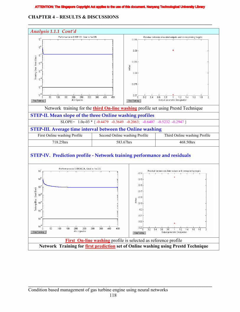
CHAPTER 4 – RESULTS & DISCUSSIONS ______________________________________________________________________________
Analysis 1.1.1 Cont’d
Network training for the third On-line washing profile set using Prestd Technique STEP-II. Mean slope of the three Online washing profiles
SLOPE= 1.0e-03 * { -0.4479 -0.3649 -0.2063; -0.6407 -0.5232 -0.2947 }
STEP-III. Average time interval between the Online washing First Online washing Profile Second Online washing Profile Third Online washing Profile
718.25hrs 583.67hrs 468.50hrs
STEP-IV. Prediction profile - Network training performance and residuals
First On-line washing profile is selected as reference profile Network Training for first prediction set of Online washing using Prestd Technique
______________________________________________________________________________ Condition based management of gas turbine engine using neural networks 118
ATTENTION: The Singapore Copyright Act applies to the use of this document. Nanyang Technological University Library
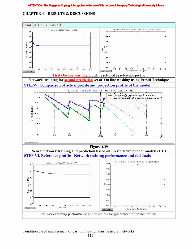
CHAPTER 4 – RESULTS & DISCUSSIONS ______________________________________________________________________________
Analysis 1.1.1 Cont’d
First On-line washing profile is selected as reference profile Network training for second prediction set of On line washing using Prestd Technique
STEP-V. Comparison of actual profile and projection profile of the model
Figure 4.29 Neural network training and prediction based on Prestd technique for analysis 1.1.1
STEP-VI. Reference profile - Network training performance and residuals
Network training performance and residuals for guaranteed reference profile
______________________________________________________________________________ Condition based management of gas turbine engine using neural networks 119
ATTENTION: The Singapore Copyright Act applies to the use of this document. Nanyang Technological University Library
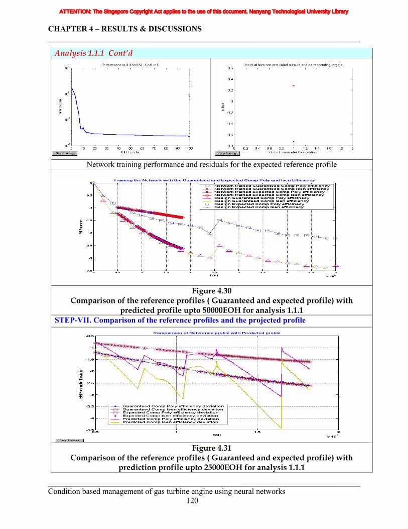
CHAPTER 4 – RESULTS & DISCUSSIONS ______________________________________________________________________________
Analysis 1.1.1 Cont’d
Network training performance and residuals for the expected reference profile
Figure 4.30 Comparison of the reference profiles ( Guaranteed and expected profile) with
predicted profile upto 50000EOH for analysis 1.1.1 STEP-VII. Comparison of the reference profiles and the projected profile
Figure 4.31
Comparison of the reference profiles ( Guaranteed and expected profile) with prediction profile upto 25000EOH for analysis 1.1.1
______________________________________________________________________________ Condition based management of gas turbine engine using neural networks 120
ATTENTION: The Singapore Copyright Act applies to the use of this document. Nanyang Technological University Library
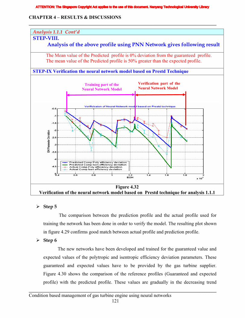
CHAPTER 4 – RESULTS & DISCUSSIONS ______________________________________________________________________________
Analysis 1.1.1 Cont’d STEP-VIII.
Analysis of the above profile using PNN Network gives following result The Mean value of the Predicted profile is 0% deviation from the guaranteed profile. The mean value of the Predicted profile is 50% greater than the expected profile. STEP-IX Verification the neural network model based on Prestd Technique
Figure 4.32
Verification of the neural network model based on Prestd technique for analysis 1.1.1
Verification part of the Neural Network Model
Training part of the Neural Network Model
Step 5
The comparison between the prediction profile and the actual profile used for
training the network has been done in order to verify the model. The resulting plot shown
in figure 4.29 confirms good match between actual profile and prediction profile.
Step 6
The new networks have been developed and trained for the guaranteed value and
expected values of the polytropic and isentropic efficiency deviation parameters. These
guaranteed and expected values have to be provided by the gas turbine supplier.
Figure 4.30 shows the comparison of the reference profiles (Guaranteed and expected
profile) with the predicted profile. These values are gradually in the decreasing trend ______________________________________________________________________________ Condition based management of gas turbine engine using neural networks 121
ATTENTION: The Singapore Copyright Act applies to the use of this document. Nanyang Technological University Library
CHAPTER 4 – RESULTS & DISCUSSIONS ______________________________________________________________________________
from 0 to 25000 EOH. At 25000 EOH the major inspection of the gas turbine is to be
done. During this inspection, some of the recoverable losses which could be retrieved
only by casing cover lift are retrieved. Therefore there is a sharp raise at this point. After
this point, it again starts to move in the gradual decrement path.
Step 7
The above network represents the values for the inputs from 0 to 50000 EOH.
From these network, the values for the operating range of the model ie 4800 EOH to
18200 EOH is simulated. Figure 4.31 shows the plot of the reference (guaranteed and
expected values) against the polytropic and isentropic efficiency deviation for the
operating range of the model. (ie from 4800 EOH to 18200 EOH).
Step 8
The predicted polytropic and isentropic efficiencies have been compared with
their respective guaranteed and expected values using PNN network. The result of the
PNN analysis indicates that the predicted profile of the polytropic and isentropic
efficiencies from 12250 EOH to 18200 EOH is almost equal to the guaranteed profile and
50% higher (adverse side) than the expected degradation profile. The above result
indicates that the gas turbine is just operating at its guaranteed profile and well above
(adverse side) the expected degradation profile.
Step 9
The verification of the neural network model has been done at this step. The
model is developed by using the actual polytropic and isentropic efficiencies degradation
values from 4800 EOH to 12250 EOH hours. The verification of the network has been
done from 12250 EOH to the 18200 EOH, in this part the actual values are fully hidden
from the model training part. The inputs to the network are given in such a way that it
will represent the actual inputs like average time interval between the on-line washing is
about 720 EOH and one off-line washing is to be carried out at 16500 EOH. The outputs
from the model and actual output from the gas turbine has been plotted in figure 4.32 as
part of model verification. The figure 4.32 shows the model is good replica of the actual
system.
______________________________________________________________________________ Condition based management of gas turbine engine using neural networks 122
ATTENTION: The Singapore Copyright Act applies to the use of this document. Nanyang Technological University Library
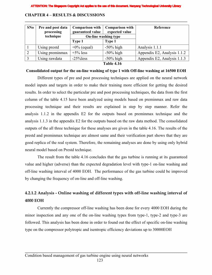
CHAPTER 4 – RESULTS & DISCUSSIONS ______________________________________________________________________________
Comparison with guaranteed value
Comparison with expected value
On-line washing type
SNo Pre and post data processing technique
Type 1 Type 1
Reference
1 Using prestd +0% (equal) -50% high Analysis 1.1.1 2 Using preminmax +5% less -50% high Appendix E2, Analysis 1.1.2 3 Using rawdata -25%less -50% high Appendix E2, Analysis 1.1.3
Table 4.16
Consolidated output for the on-line washing of type 1 with Off-line washing at 16500 EOH
Different types of pre and post processing techniques are applied on the neural network
model inputs and targets in order to make their training more efficient for getting the desired
results. In order to select the particular pre and post processing techniques, the data from the first
column of the table 4.15 have been analyzed using models based on preminmax and raw data
processing technique and their results are explained in step by step manner. Refer the
analysis 1.1.2 in the appendix E2 for the outputs based on preminmax technique and the
analysis 1.1.3 in the appendix E2 for the outputs based on the raw data method. The consolidated
outputs of the all three technique for these analyses are given in the table 4.16. The results of the
prestd and preminmax technique are almost same and their verification part shows that they are
good replica of the real system. Therefore, the remaining analyses are done by using only hybrid
neural model based on Prestd technique.
The result from the table 4.16 concludes that the gas turbine is running at its guaranteed
value and higher (adverse) than the expected degradation level with type-1 on-line washing and
off-line washing interval of 4000 EOH. The performance of the gas turbine could be improved
by changing the frequency of on-line and off-line washing.
4.2.1.2 Analysis - Online washing of different types with off-line washing interval of
4000 EOH
Currently the compressor off-line washing has been done for every 4000 EOH during the
minor inspection and any one of the on-line washing types from type-1, type-2 and type-3 are
followed. This analysis has been done in order to found out the effect of specific on-line washing
type on the compressor polytropic and isentropic efficiency deviations up to 30000EOH
______________________________________________________________________________ Condition based management of gas turbine engine using neural networks 123
ATTENTION: The Singapore Copyright Act applies to the use of this document. Nanyang Technological University Library
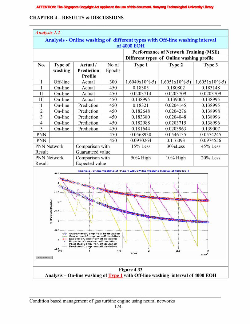
CHAPTER 4 – RESULTS & DISCUSSIONS ______________________________________________________________________________
Analysis 1.2 Analysis - Online washing of different types with Off-line washing interval
of 4000 EOH Performance of Network Training (MSE)
Different types of Online washing profile No. Type of
washing Actual /
Prediction Profile
No of Epochs
Type 1 Type 2 Type 3
I Off-line Actual 300 1.6049x10^(-5) 1.6051x10^(-5) 1.6051x10^(-5)I On-line Actual 450 0.18305 0.180802 0.183148 II On-line Actual 450 0.0203714 0.0203709 0.0203709 III On-line Actual 450 0.138995 0.139005 0.138995 1 On-line Prediction 450 0.18321 0.0204145 0.138995 2 On-line Prediction 450 0.182648 0.0204276 0.138998 3 On-line Prediction 450 0.183380 0.0204048 0.138996 4 On-line Prediction 450 0.182988 0.0203715 0.138996 5 On-line Prediction 450 0.181644 0.0203963 0.139007
PNN 450 0.0568930 0.0546135 0.0574245 PNN 450 0.0970264 0.116093 0.0974556 PNN Network Result
Comparison with Guaranteed value
15% Less 30%Less 45% Less
PNN Network Result
Comparison with Expected value
50% High 10% High 20% Less
Figure 4.33 Analysis – On-line washing of Type 1 with Off-line washing interval of 4000 EOH
______________________________________________________________________________ Condition based management of gas turbine engine using neural networks 124
ATTENTION: The Singapore Copyright Act applies to the use of this document. Nanyang Technological University Library
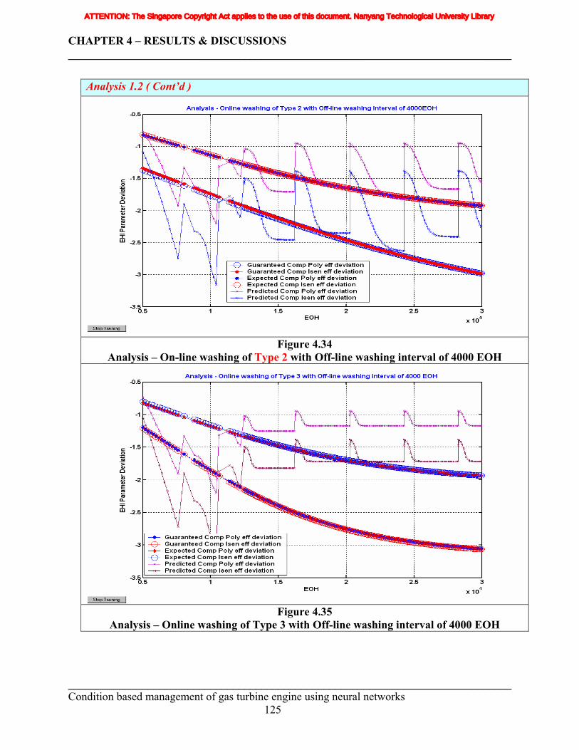
CHAPTER 4 – RESULTS & DISCUSSIONS ______________________________________________________________________________
Analysis 1.2 ( Cont’d )
Figure 4.34
Analysis – On-line washing of Type 2 with Off-line washing interval of 4000 EOH
Figure 4.35
Analysis – Online washing of Type 3 with Off-line washing interval of 4000 EOH
______________________________________________________________________________ Condition based management of gas turbine engine using neural networks 125
ATTENTION: The Singapore Copyright Act applies to the use of this document. Nanyang Technological University Library
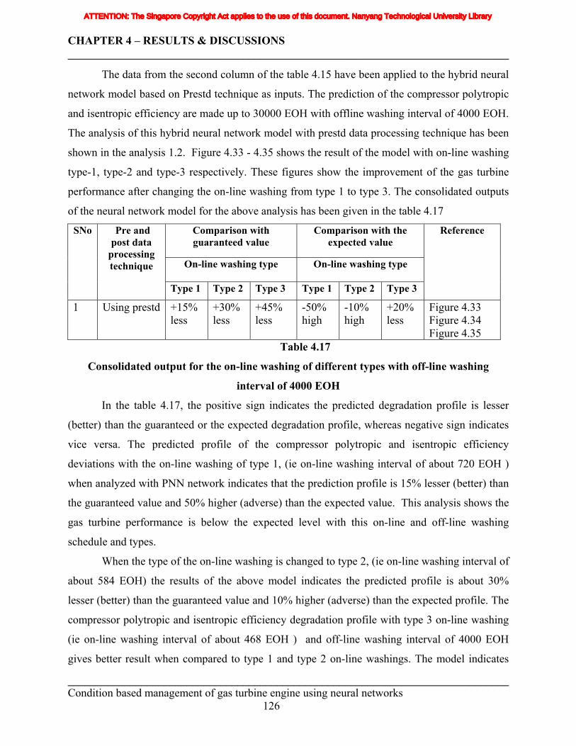
CHAPTER 4 – RESULTS & DISCUSSIONS ______________________________________________________________________________
The data from the second column of the table 4.15 have been applied to the hybrid neural
network model based on Prestd technique as inputs. The prediction of the compressor polytropic
and isentropic efficiency are made up to 30000 EOH with offline washing interval of 4000 EOH.
The analysis of this hybrid neural network model with prestd data processing technique has been
shown in the analysis 1.2. Figure 4.33 - 4.35 shows the result of the model with on-line washing
type-1, type-2 and type-3 respectively. These figures show the improvement of the gas turbine
performance after changing the on-line washing from type 1 to type 3. The consolidated outputs
of the neural network model for the above analysis has been given in the table 4.17
Comparison with guaranteed value
Comparison with the expected value
On-line washing type On-line washing type
SNo Pre and post data
processing technique
Type 1 Type 2 Type 3 Type 1 Type 2 Type 3
Reference
1 Using prestd +15% less
+30% less
+45% less
-50% high
-10% high
+20% less
Figure 4.33 Figure 4.34 Figure 4.35
Table 4.17
Consolidated output for the on-line washing of different types with off-line washing
interval of 4000 EOH
In the table 4.17, the positive sign indicates the predicted degradation profile is lesser
(better) than the guaranteed or the expected degradation profile, whereas negative sign indicates
vice versa. The predicted profile of the compressor polytropic and isentropic efficiency
deviations with the on-line washing of type 1, (ie on-line washing interval of about 720 EOH )
when analyzed with PNN network indicates that the prediction profile is 15% lesser (better) than
the guaranteed value and 50% higher (adverse) than the expected value. This analysis shows the
gas turbine performance is below the expected level with this on-line and off-line washing
schedule and types.
When the type of the on-line washing is changed to type 2, (ie on-line washing interval of
about 584 EOH) the results of the above model indicates the predicted profile is about 30%
lesser (better) than the guaranteed value and 10% higher (adverse) than the expected profile. The
compressor polytropic and isentropic efficiency degradation profile with type 3 on-line washing
(ie on-line washing interval of about 468 EOH ) and off-line washing interval of 4000 EOH
gives better result when compared to type 1 and type 2 on-line washings. The model indicates
______________________________________________________________________________ Condition based management of gas turbine engine using neural networks 126
ATTENTION: The Singapore Copyright Act applies to the use of this document. Nanyang Technological University Library
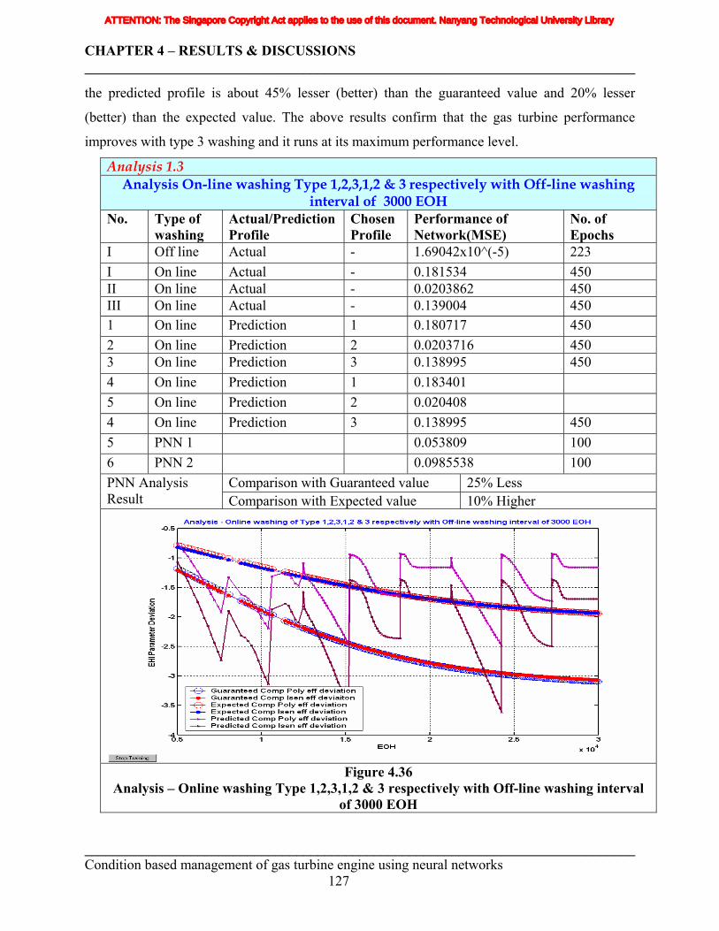
CHAPTER 4 – RESULTS & DISCUSSIONS ______________________________________________________________________________
the predicted profile is about 45% lesser (better) than the guaranteed value and 20% lesser
(better) than the expected value. The above results confirm that the gas turbine performance
improves with type 3 washing and it runs at its maximum performance level.
Analysis 1.3 Analysis On-line washing Type 1,2,3,1,2 & 3 respectively with Off-line washing
interval of 3000 EOH No. Type of
washing Actual/Prediction Profile
Chosen Profile
Performance of Network(MSE)
No. of Epochs
I Off line Actual - 1.69042x10^(-5) 223 I On line Actual - 0.181534 450 II On line Actual - 0.0203862 450 III On line Actual - 0.139004 450 1 On line Prediction 1 0.180717 450 2 On line Prediction 2 0.0203716 450 3 On line Prediction 3 0.138995 450 4 On line Prediction 1 0.183401 5 On line Prediction 2 0.020408 4 On line Prediction 3 0.138995 450 5 PNN 1 0.053809 100 6 PNN 2 0.0985538 100
Comparison with Guaranteed value 25% Less PNN Analysis Result Comparison with Expected value 10% Higher
Figure 4.36
Analysis – Online washing Type 1,2,3,1,2 & 3 respectively with Off-line washing interval of 3000 EOH
______________________________________________________________________________ Condition based management of gas turbine engine using neural networks 127
ATTENTION: The Singapore Copyright Act applies to the use of this document. Nanyang Technological University Library
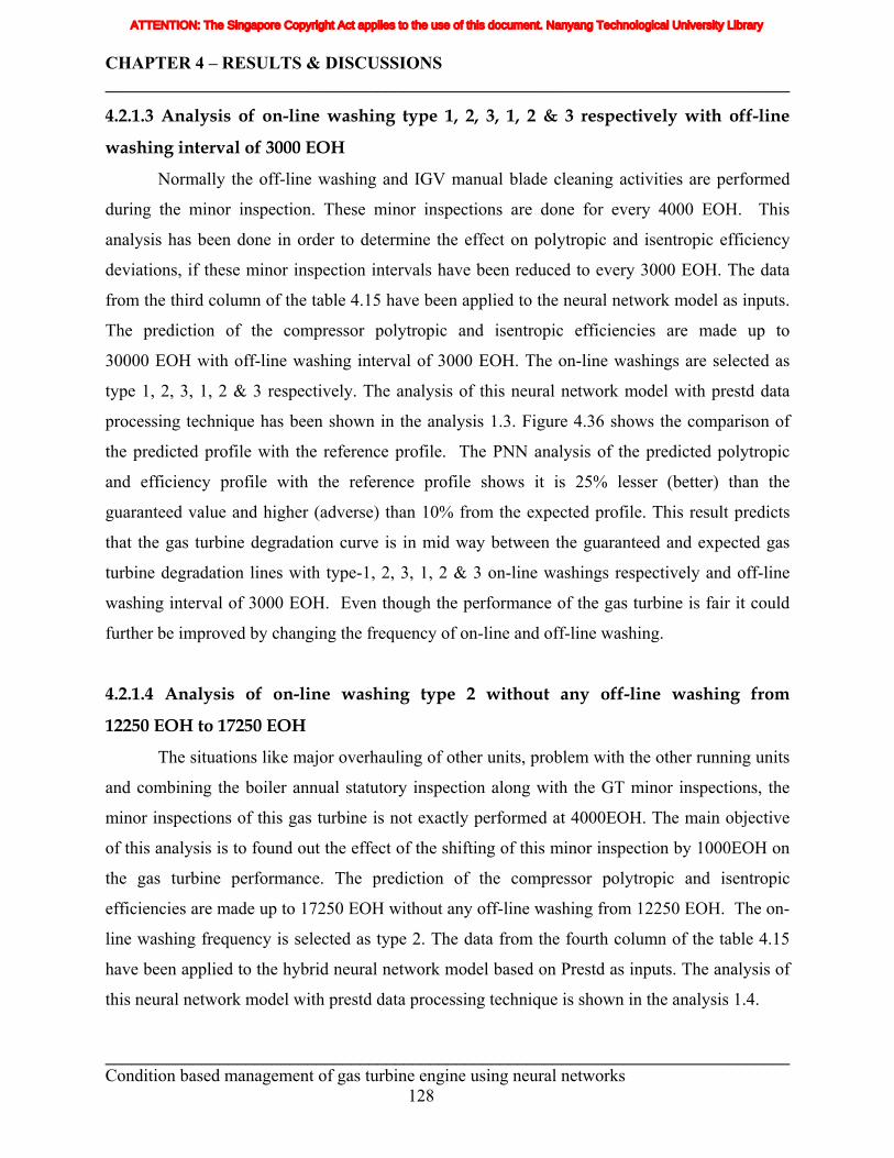
CHAPTER 4 – RESULTS & DISCUSSIONS ______________________________________________________________________________
4.2.1.3 Analysis of on-line washing type 1, 2, 3, 1, 2 & 3 respectively with off-line
washing interval of 3000 EOH
Normally the off-line washing and IGV manual blade cleaning activities are performed
during the minor inspection. These minor inspections are done for every 4000 EOH. This
analysis has been done in order to determine the effect on polytropic and isentropic efficiency
deviations, if these minor inspection intervals have been reduced to every 3000 EOH. The data
from the third column of the table 4.15 have been applied to the neural network model as inputs.
The prediction of the compressor polytropic and isentropic efficiencies are made up to
30000 EOH with off-line washing interval of 3000 EOH. The on-line washings are selected as
type 1, 2, 3, 1, 2 & 3 respectively. The analysis of this neural network model with prestd data
processing technique has been shown in the analysis 1.3. Figure 4.36 shows the comparison of
the predicted profile with the reference profile. The PNN analysis of the predicted polytropic
and efficiency profile with the reference profile shows it is 25% lesser (better) than the
guaranteed value and higher (adverse) than 10% from the expected profile. This result predicts
that the gas turbine degradation curve is in mid way between the guaranteed and expected gas
turbine degradation lines with type-1, 2, 3, 1, 2 & 3 on-line washings respectively and off-line
washing interval of 3000 EOH. Even though the performance of the gas turbine is fair it could
further be improved by changing the frequency of on-line and off-line washing.
4.2.1.4 Analysis of on-line washing type 2 without any off-line washing from
12250 EOH to 17250 EOH
The situations like major overhauling of other units, problem with the other running units
and combining the boiler annual statutory inspection along with the GT minor inspections, the
minor inspections of this gas turbine is not exactly performed at 4000EOH. The main objective
of this analysis is to found out the effect of the shifting of this minor inspection by 1000EOH on
the gas turbine performance. The prediction of the compressor polytropic and isentropic
efficiencies are made up to 17250 EOH without any off-line washing from 12250 EOH. The on-
line washing frequency is selected as type 2. The data from the fourth column of the table 4.15
have been applied to the hybrid neural network model based on Prestd as inputs. The analysis of
this neural network model with prestd data processing technique is shown in the analysis 1.4.
______________________________________________________________________________ Condition based management of gas turbine engine using neural networks 128
ATTENTION: The Singapore Copyright Act applies to the use of this document. Nanyang Technological University Library
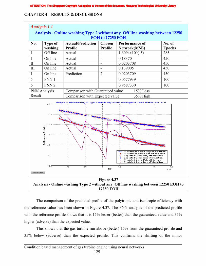
CHAPTER 4 – RESULTS & DISCUSSIONS ______________________________________________________________________________
Analysis 1.4 Analysis - Online washing Type 2 without any Off line washing between 12250
EOH to 17250 EOH No. Type of
washing Actual/Prediction Profile
Chosen Profile
Performance of Network(MSE)
No. of Epochs
I Off line Actual - 1.6094x10^(-5) 285 I On line Actual - 0.18370 450 II On line Actual - 0.0203708 450 III On line Actual - 0.139005 450 1 On line Prediction 2 0.0203709 450 5 PNN 1 0.0577939 100 6 PNN 2 0.9587330 100
Comparison with Guaranteed value 15% Less PNN Analysis Result Comparison with Expected value 35% High
Figure 4.37 Analysis - Online washing Type 2 without any Off line washing between 12250 EOH to
17250 EOH
The comparison of the predicted profile of the polytropic and isentropic efficiency with
the reference value has been shown in Figure 4.37. The PNN analysis of the predicted profile
with the reference profile shows that it is 15% lesser (better) than the guaranteed value and 35%
higher (adverse) than the expected value.
This shows that the gas turbine run above (better) 15% from the guaranteed profile and
35% below (adverse) than the expected profile. This confirms the shifting of the minor
______________________________________________________________________________ Condition based management of gas turbine engine using neural networks 129
ATTENTION: The Singapore Copyright Act applies to the use of this document. Nanyang Technological University Library
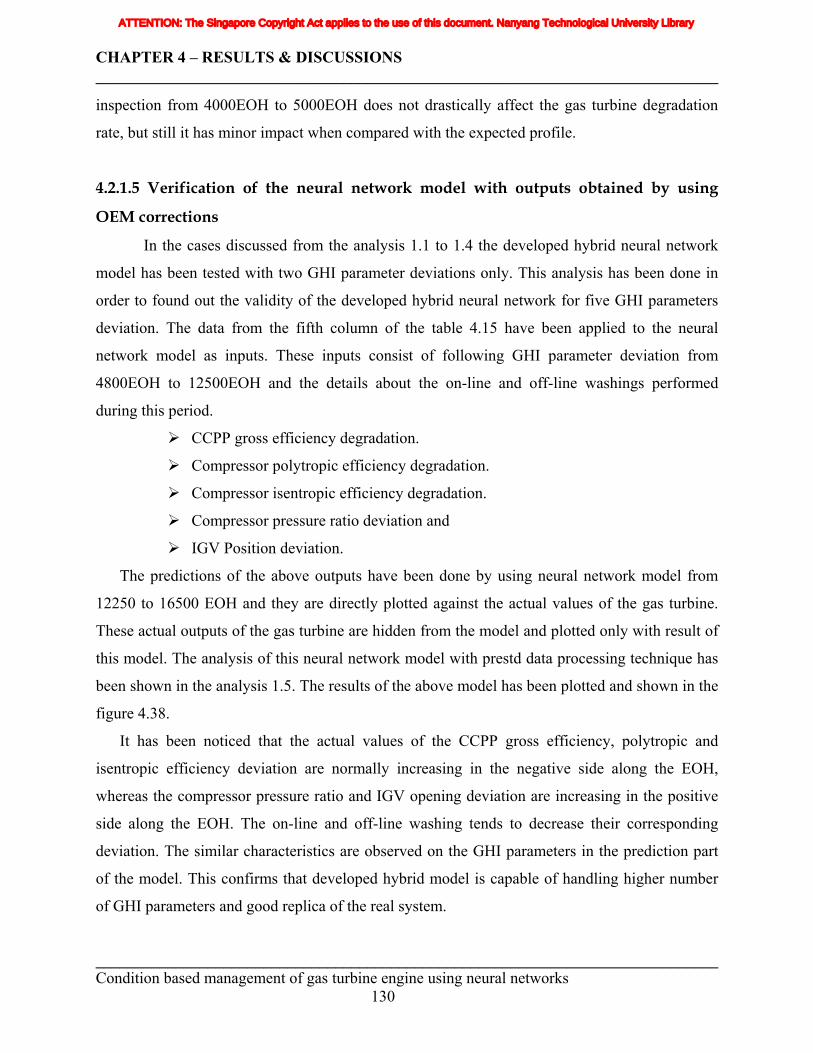
CHAPTER 4 – RESULTS & DISCUSSIONS ______________________________________________________________________________
inspection from 4000EOH to 5000EOH does not drastically affect the gas turbine degradation
rate, but still it has minor impact when compared with the expected profile.
4.2.1.5 Verification of the neural network model with outputs obtained by using
OEM corrections
In the cases discussed from the analysis 1.1 to 1.4 the developed hybrid neural network
model has been tested with two GHI parameter deviations only. This analysis has been done in
order to found out the validity of the developed hybrid neural network for five GHI parameters
deviation. The data from the fifth column of the table 4.15 have been applied to the neural
network model as inputs. These inputs consist of following GHI parameter deviation from
4800EOH to 12500EOH and the details about the on-line and off-line washings performed
during this period.
CCPP gross efficiency degradation.
Compressor polytropic efficiency degradation.
Compressor isentropic efficiency degradation.
Compressor pressure ratio deviation and
IGV Position deviation.
The predictions of the above outputs have been done by using neural network model from
12250 to 16500 EOH and they are directly plotted against the actual values of the gas turbine.
These actual outputs of the gas turbine are hidden from the model and plotted only with result of
this model. The analysis of this neural network model with prestd data processing technique has
been shown in the analysis 1.5. The results of the above model has been plotted and shown in the
figure 4.38.
It has been noticed that the actual values of the CCPP gross efficiency, polytropic and
isentropic efficiency deviation are normally increasing in the negative side along the EOH,
whereas the compressor pressure ratio and IGV opening deviation are increasing in the positive
side along the EOH. The on-line and off-line washing tends to decrease their corresponding
deviation. The similar characteristics are observed on the GHI parameters in the prediction part
of the model. This confirms that developed hybrid model is capable of handling higher number
of GHI parameters and good replica of the real system.
______________________________________________________________________________ Condition based management of gas turbine engine using neural networks 130
ATTENTION: The Singapore Copyright Act applies to the use of this document. Nanyang Technological University Library
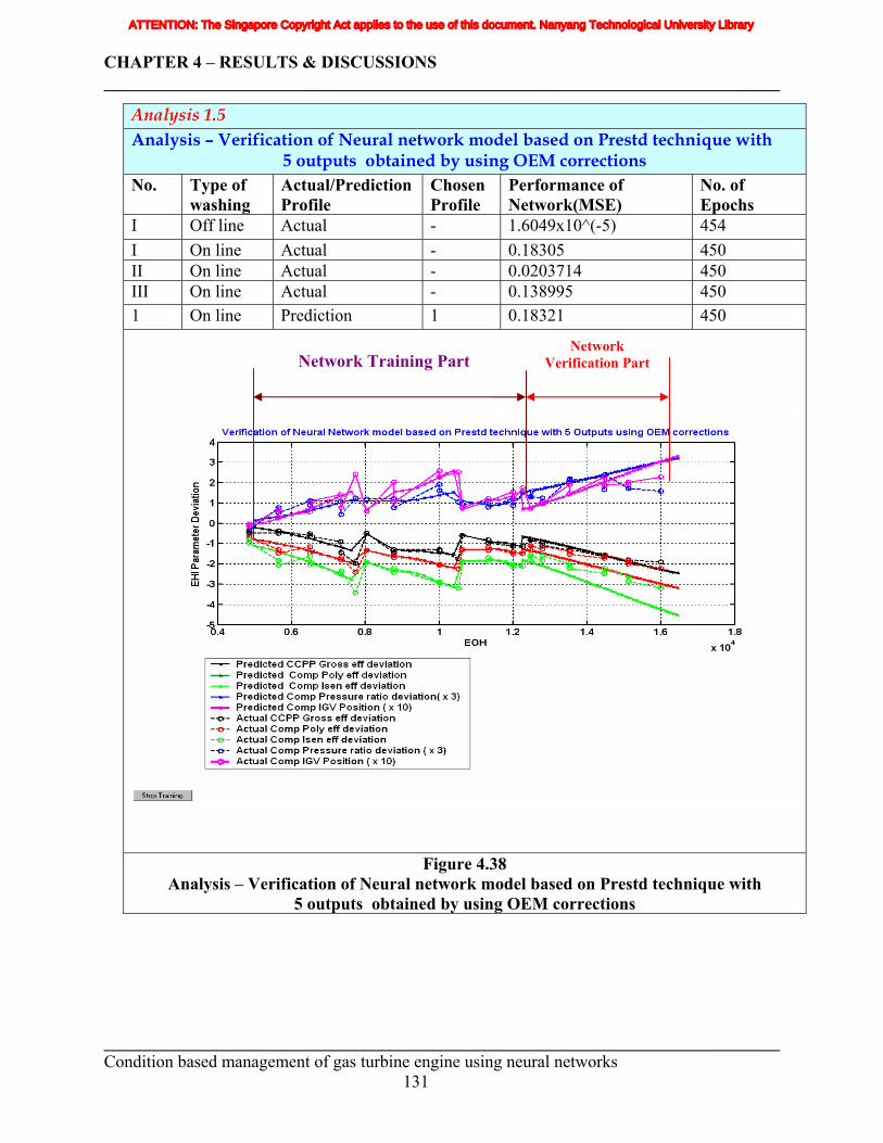
CHAPTER 4 – RESULTS & DISCUSSIONS ______________________________________________________________________________
Analysis 1.5 Analysis – Verification of Neural network model based on Prestd technique with
5 outputs obtained by using OEM corrections No. Type of
washing Actual/Prediction Profile
Chosen Profile
Performance of Network(MSE)
No. of Epochs
I Off line Actual - 1.6049x10^(-5) 454 I On line Actual - 0.18305 450 II On line Actual - 0.0203714 450 III On line Actual - 0.138995 450 1 On line Prediction 1 0.18321 450
Figure 4.38 Analysis – Verification of Neural network model based on Prestd technique with
5 outputs obtained by using OEM corrections
Network Verification Part Network Training Part
______________________________________________________________________________ Condition based management of gas turbine engine using neural networks 131
ATTENTION: The Singapore Copyright Act applies to the use of this document. Nanyang Technological University Library
CHAPTER 4 – RESULTS & DISCUSSIONS ______________________________________________________________________________
Analysis 1.6 Analysis – Verification of Neural network model based on Prestd technique with
5 outputs obtained by using STD corrections No. Type of
washing Actual/Prediction Profile
Chosen Profile
Performance of Network(MSE)
No. of Epochs
I Off line Actual - 1.6049 x 10^(-5) 326 I On line Actual - 0.18235 450 II On line Actual - 0.0192314 450 III On line Actual - 0.148794 450 1 On line Prediction 1 0.179322 450
Figure 4.39 Analysis – Verification of Neural network model based on Prestd technique with
5 outputs obtained by using STD corrections
Network Verification part Network training part
______________________________________________________________________________ Condition based management of gas turbine engine using neural networks 132
ATTENTION: The Singapore Copyright Act applies to the use of this document. Nanyang Technological University Library
CHAPTER 4 – RESULTS & DISCUSSIONS ______________________________________________________________________________
4.2.1.6 Verification of the neural network model with outputs obtained by using the
STD corrections.
The developed hybrid neural network model has applied to predict the behavior of the gas
turbine degradation rate based on OEM corrections in the analysis 1.1 to 1.5. In order to verify
the capability of this model to handling the GHI parameters deviation based on the STD
correction this analysis has been done. The input data from the sixth column of the table 4.15
have been applied to the neural network model as inputs. These inputs consist of CCPP gross,
polytropic, isentropic efficiency, CDT and IGV position deviation respectively from 4800 EOH
to 12500 EOH and corresponding on-line and off-line washings performed. The prediction of
the network has been done from 12250 EOH to 16500EOH with on-line washing of type-1 and
without any off-line washing. The outputs of this analysis are shown in the analysis 1.6. The
predicted outputs of the above analysis is plotted against the actual values of the GHI parameters
deviation and shown in Figure 4.39.
The actual outputs of the GHI parameter deviation from 12250 to 16500EOH are hidden
from the model training part and plotted only with result of the model. The figure 4.39 shows
that predicted values of GHI parameter deviation behave in similar manner like the actual values
hidden from the training of this model. This confirms the model is a good replica of the real
system and has the capability of handing the GHI parameters based on STD corrections also.
4.2.2 Thermo-Economical assessment of gas turbine engine using the
hybrid neural network models The result of the thermal analyses show that the hybrid neural network model based on
prestd and preminmax data processing techniques are the good replica of the real system. The
neural network model based on prestd data processing technique is taken for cost analysis of the
gas turbine engine degradation. The cost analysis of the system has been done using the CCPP
gross efficiency degradation alone. The guaranteed degradation curve represents the minimum
possible performance of the gas turbine and expected degradation curve represents the maximum
possible performance of the gas turbine. Even though the comparison has been made between the
guaranteed profile and predicted profile, the cost analysis has been done only based on the
comparison between the predicted profile and expected profile.
______________________________________________________________________________ Condition based management of gas turbine engine using neural networks 133
ATTENTION: The Singapore Copyright Act applies to the use of this document. Nanyang Technological University Library
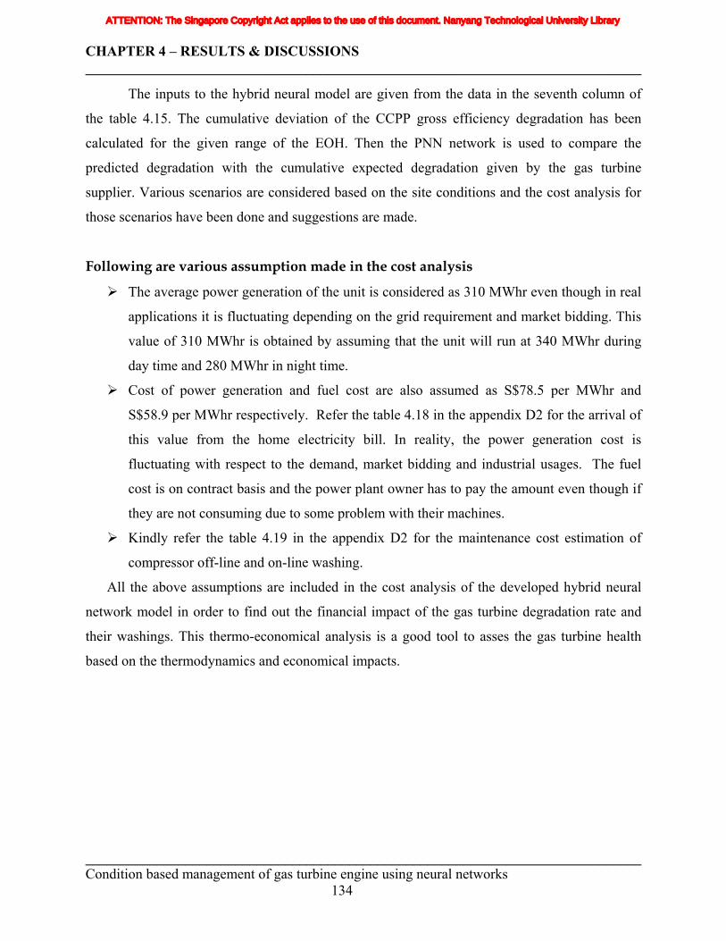
CHAPTER 4 – RESULTS & DISCUSSIONS ______________________________________________________________________________
The inputs to the hybrid neural model are given from the data in the seventh column of
the table 4.15. The cumulative deviation of the CCPP gross efficiency degradation has been
calculated for the given range of the EOH. Then the PNN network is used to compare the
predicted degradation with the cumulative expected degradation given by the gas turbine
supplier. Various scenarios are considered based on the site conditions and the cost analysis for
those scenarios have been done and suggestions are made.
Following are various assumption made in the cost analysis
The average power generation of the unit is considered as 310 MWhr even though in real
applications it is fluctuating depending on the grid requirement and market bidding. This
value of 310 MWhr is obtained by assuming that the unit will run at 340 MWhr during
day time and 280 MWhr in night time.
Cost of power generation and fuel cost are also assumed as S$78.5 per MWhr and
S$58.9 per MWhr respectively. Refer the table 4.18 in the appendix D2 for the arrival of
this value from the home electricity bill. In reality, the power generation cost is
fluctuating with respect to the demand, market bidding and industrial usages. The fuel
cost is on contract basis and the power plant owner has to pay the amount even though if
they are not consuming due to some problem with their machines.
Kindly refer the table 4.19 in the appendix D2 for the maintenance cost estimation of
compressor off-line and on-line washing.
All the above assumptions are included in the cost analysis of the developed hybrid neural
network model in order to find out the financial impact of the gas turbine degradation rate and
their washings. This thermo-economical analysis is a good tool to asses the gas turbine health
based on the thermodynamics and economical impacts.
______________________________________________________________________________ Condition based management of gas turbine engine using neural networks 134
ATTENTION: The Singapore Copyright Act applies to the use of this document. Nanyang Technological University Library
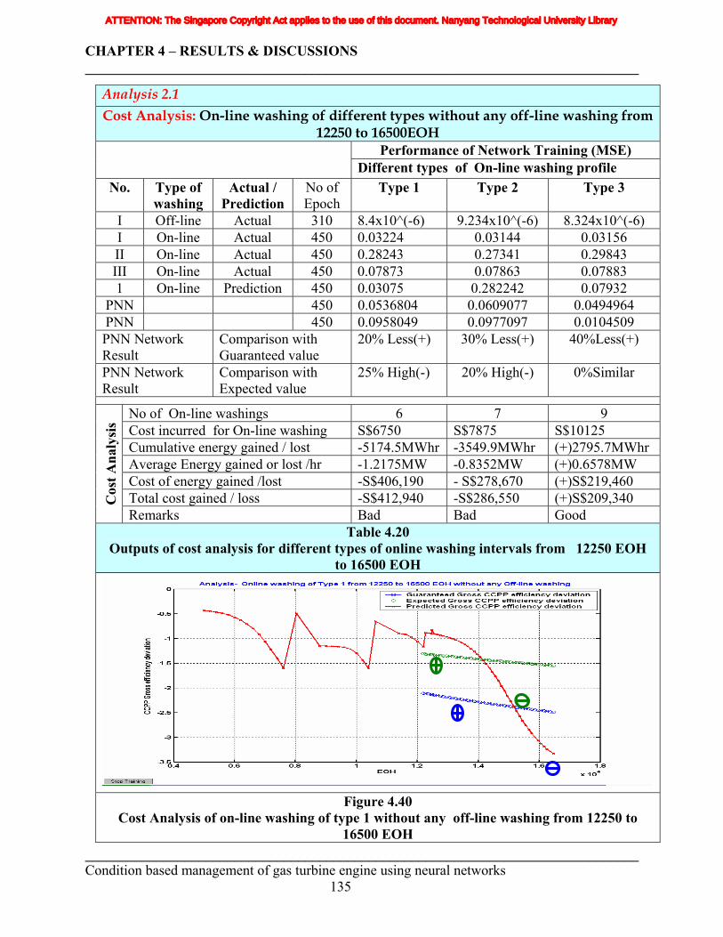
CHAPTER 4 – RESULTS & DISCUSSIONS ______________________________________________________________________________
Analysis 2.1 Cost Analysis: On-line washing of different types without any off-line washing from
12250 to 16500EOH Performance of Network Training (MSE)
Different types of On-line washing profile No. Type of
washing Actual /
Prediction No of Epoch
Type 1 Type 2 Type 3
I Off-line Actual 310 8.4x10^(-6) 9.234x10^(-6) 8.324x10^(-6) I On-line Actual 450 0.03224 0.03144 0.03156 II On-line Actual 450 0.28243 0.27341 0.29843 III On-line Actual 450 0.07873 0.07863 0.07883 1 On-line Prediction 450 0.03075 0.282242 0.07932
PNN 450 0.0536804 0.0609077 0.0494964 PNN 450 0.0958049 0.0977097 0.0104509 PNN Network Result
Comparison with Guaranteed value
20% Less(+) 30% Less(+) 40%Less(+)
PNN Network Result
Comparison with Expected value
25% High(-) 20% High(-) 0%Similar
No of On-line washings 6 7 9 Cost incurred for On-line washing S$6750 S$7875 S$10125 Cumulative energy gained / lost -5174.5MWhr -3549.9MWhr (+)2795.7MWhr Average Energy gained or lost /hr -1.2175MW -0.8352MW (+)0.6578MW Cost of energy gained /lost -S$406,190 - S$278,670 (+)S$219,460 Total cost gained / loss -S$412,940 -S$286,550 (+)S$209,340 C
ost A
naly
sis
Remarks Bad Bad Good Table 4.20
Outputs of cost analysis for different types of online washing intervals from 12250 EOH to 16500 EOH
Figure 4.40 Cost Analysis of on-line washing of type 1 without any off-line washing from 12250 to
16500 EOH ______________________________________________________________________________ Condition based management of gas turbine engine using neural networks 135
ATTENTION: The Singapore Copyright Act applies to the use of this document. Nanyang Technological University Library
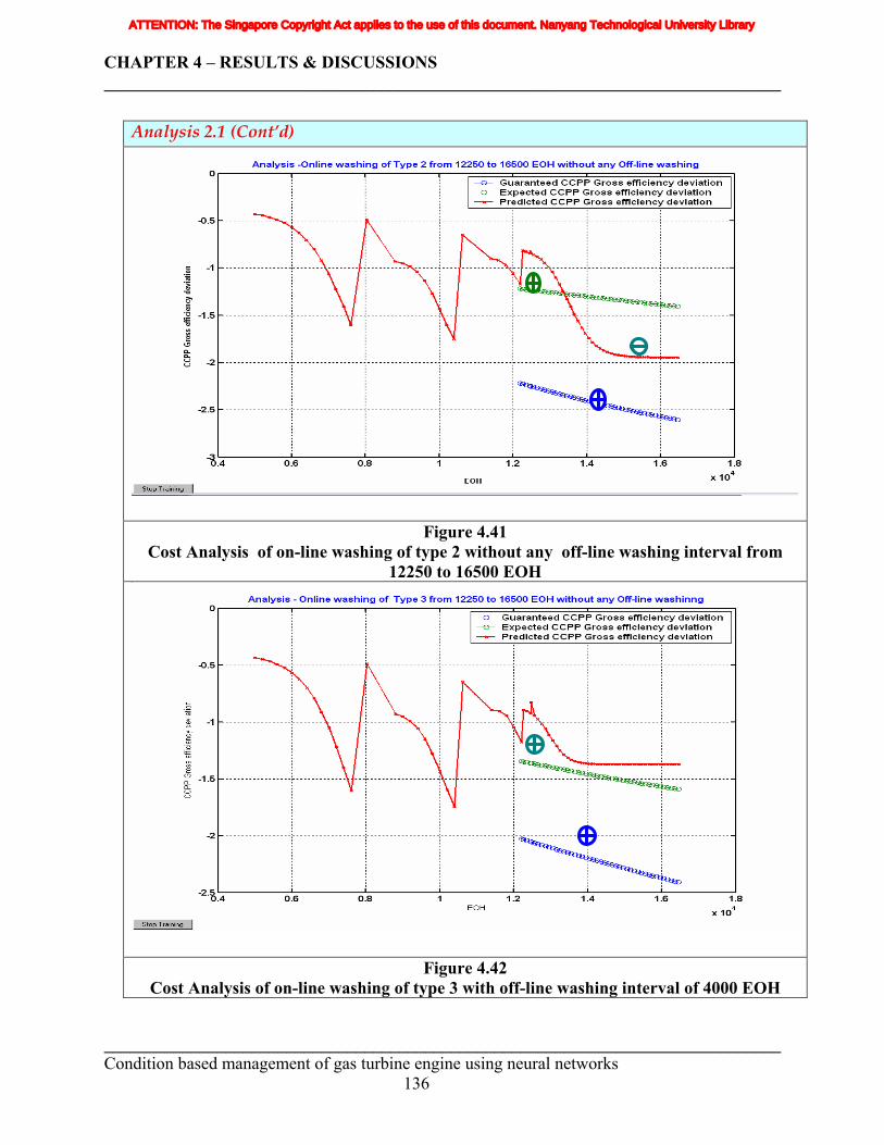
CHAPTER 4 – RESULTS & DISCUSSIONS ______________________________________________________________________________
Analysis 2.1 (Cont’d)
Figure 4.41 Cost Analysis of on-line washing of type 2 without any off-line washing interval from
12250 to 16500 EOH
Figure 4.42 Cost Analysis of on-line washing of type 3 with off-line washing interval of 4000 EOH
______________________________________________________________________________ Condition based management of gas turbine engine using neural networks 136
ATTENTION: The Singapore Copyright Act applies to the use of this document. Nanyang Technological University Library
CHAPTER 4 – RESULTS & DISCUSSIONS ______________________________________________________________________________
4.2.2.1 Cost analysis of different types of on-line washing without any off-line
washing from 12250 to 16250 EOH
Normally the minor inspection of the gas turbine is done for every 4000 EOH.
(Approximately 5.5 months). So the cost analysis has been done for this scenario considering
various types of on-line washing frequency.
Type-1 refers that one on-line washing is performed for every 720 EOH.
Type-2 refers that one on-line washing is performed for every 584 EOH.
Type-3 refers that one on-line washing is performed for every 470 EOH
The data from the seventh column of the table 4.15 have been given as input to the hybrid
neural network model based on prestd technique. These consists of CCPP gross efficiency
deviation based on OEM corrections from 4800 EOH to 12500 EOH and various on-line & off-
line washing performed during this period. The outputs of this model are shown in the
analysis 2.1.
The intersection point of the predicted CCPP gross efficiency degradation profile with the
expected efficiency degradation profile is the ideal period for doing the off-line washing.
Figures 4.40 and 4.41 in the analysis 2.1 shows that if on-line washing frequency is followed as
type 1 and type 2 intervals, the offline washing to be done at 14250 EOH without considering the
power generation opportunity cost lost. If the lost of opportunity cost is considered the position
would be shifted, this analysis has been done in the later scenarios.
Figure 4.42 in the analysis 2.1 shows that the type 3 online-washing interval maintains
the degradation profile in-line with the expected degradation profile without any off-line
washing. The table 4.20 in the analysis shows that the type 3 on-line washing interval gives
better result when compared with the type 1 and type 2. This cost analysis also shows that the
average energy lost per hour is of very small range from -1.2 MW to +0.65MW, but their
cumulative cost effect for the overall period is very high.
______________________________________________________________________________ Condition based management of gas turbine engine using neural networks 137
ATTENTION: The Singapore Copyright Act applies to the use of this document. Nanyang Technological University Library
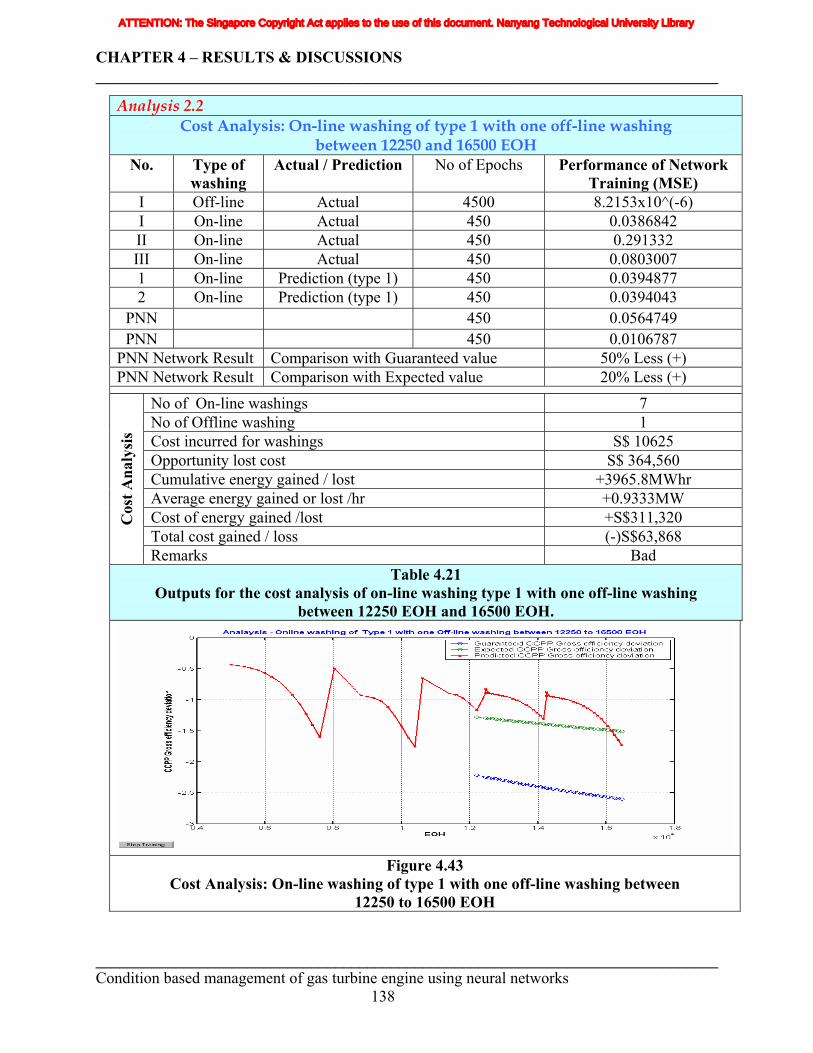
CHAPTER 4 – RESULTS & DISCUSSIONS ______________________________________________________________________________
Analysis 2.2 Cost Analysis: On-line washing of type 1 with one off-line washing
between 12250 and 16500 EOH No. Type of
washing Actual / Prediction No of Epochs Performance of Network
Training (MSE) I Off-line Actual 4500 8.2153x10^(-6) I On-line Actual 450 0.0386842 II On-line Actual 450 0.291332 III On-line Actual 450 0.0803007 1 On-line Prediction (type 1) 450 0.0394877 2 On-line Prediction (type 1) 450 0.0394043
PNN 450 0.0564749 PNN 450 0.0106787
PNN Network Result Comparison with Guaranteed value 50% Less (+) PNN Network Result Comparison with Expected value 20% Less (+)
No of On-line washings 7 No of Offline washing 1 Cost incurred for washings S$ 10625 Opportunity lost cost S$ 364,560 Cumulative energy gained / lost +3965.8MWhr Average energy gained or lost /hr +0.9333MW Cost of energy gained /lost +S$311,320 Total cost gained / loss (-)S$63,868
Cos
t Ana
lysi
s
Remarks Bad Table 4.21
Outputs for the cost analysis of on-line washing type 1 with one off-line washing between 12250 EOH and 16500 EOH.
Figure 4.43
Cost Analysis: On-line washing of type 1 with one off-line washing between 12250 to 16500 EOH
______________________________________________________________________________ Condition based management of gas turbine engine using neural networks 138
ATTENTION: The Singapore Copyright Act applies to the use of this document. Nanyang Technological University Library
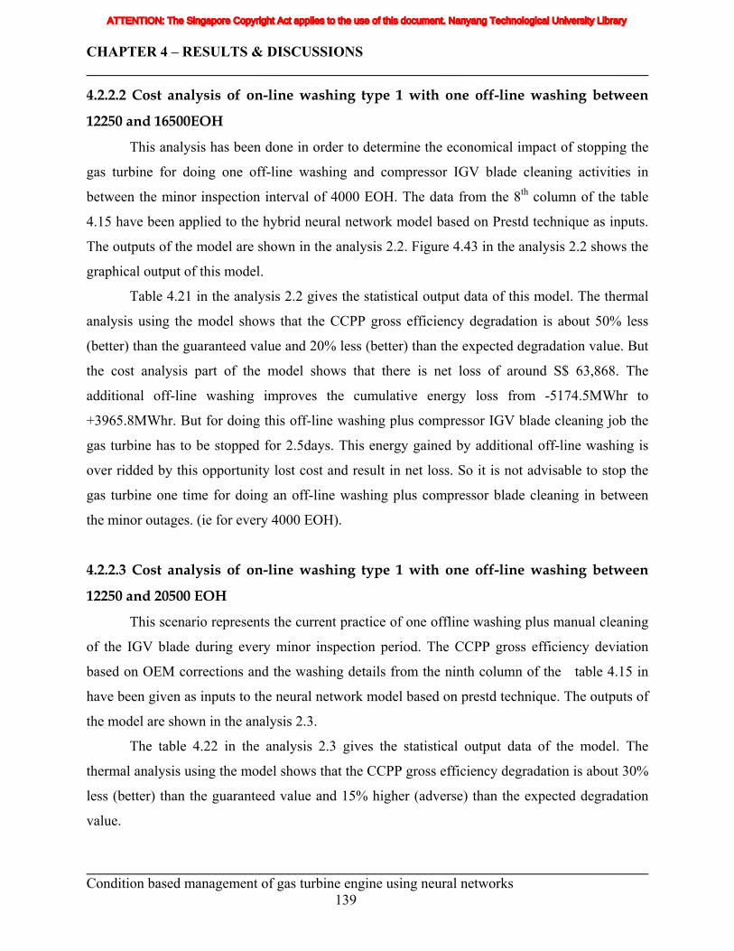
CHAPTER 4 – RESULTS & DISCUSSIONS ______________________________________________________________________________
4.2.2.2 Cost analysis of on-line washing type 1 with one off-line washing between
12250 and 16500EOH
This analysis has been done in order to determine the economical impact of stopping the
gas turbine for doing one off-line washing and compressor IGV blade cleaning activities in
between the minor inspection interval of 4000 EOH. The data from the 8th column of the table
4.15 have been applied to the hybrid neural network model based on Prestd technique as inputs.
The outputs of the model are shown in the analysis 2.2. Figure 4.43 in the analysis 2.2 shows the
graphical output of this model.
Table 4.21 in the analysis 2.2 gives the statistical output data of this model. The thermal
analysis using the model shows that the CCPP gross efficiency degradation is about 50% less
(better) than the guaranteed value and 20% less (better) than the expected degradation value. But
the cost analysis part of the model shows that there is net loss of around S$ 63,868. The
additional off-line washing improves the cumulative energy loss from -5174.5MWhr to
+3965.8MWhr. But for doing this off-line washing plus compressor IGV blade cleaning job the
gas turbine has to be stopped for 2.5days. This energy gained by additional off-line washing is
over ridded by this opportunity lost cost and result in net loss. So it is not advisable to stop the
gas turbine one time for doing an off-line washing plus compressor blade cleaning in between
the minor outages. (ie for every 4000 EOH).
4.2.2.3 Cost analysis of on-line washing type 1 with one off-line washing between
12250 and 20500 EOH
This scenario represents the current practice of one offline washing plus manual cleaning
of the IGV blade during every minor inspection period. The CCPP gross efficiency deviation
based on OEM corrections and the washing details from the ninth column of the table 4.15 in
have been given as inputs to the neural network model based on prestd technique. The outputs of
the model are shown in the analysis 2.3.
The table 4.22 in the analysis 2.3 gives the statistical output data of the model. The
thermal analysis using the model shows that the CCPP gross efficiency degradation is about 30%
less (better) than the guaranteed value and 15% higher (adverse) than the expected degradation
value.
______________________________________________________________________________ Condition based management of gas turbine engine using neural networks 139
ATTENTION: The Singapore Copyright Act applies to the use of this document. Nanyang Technological University Library
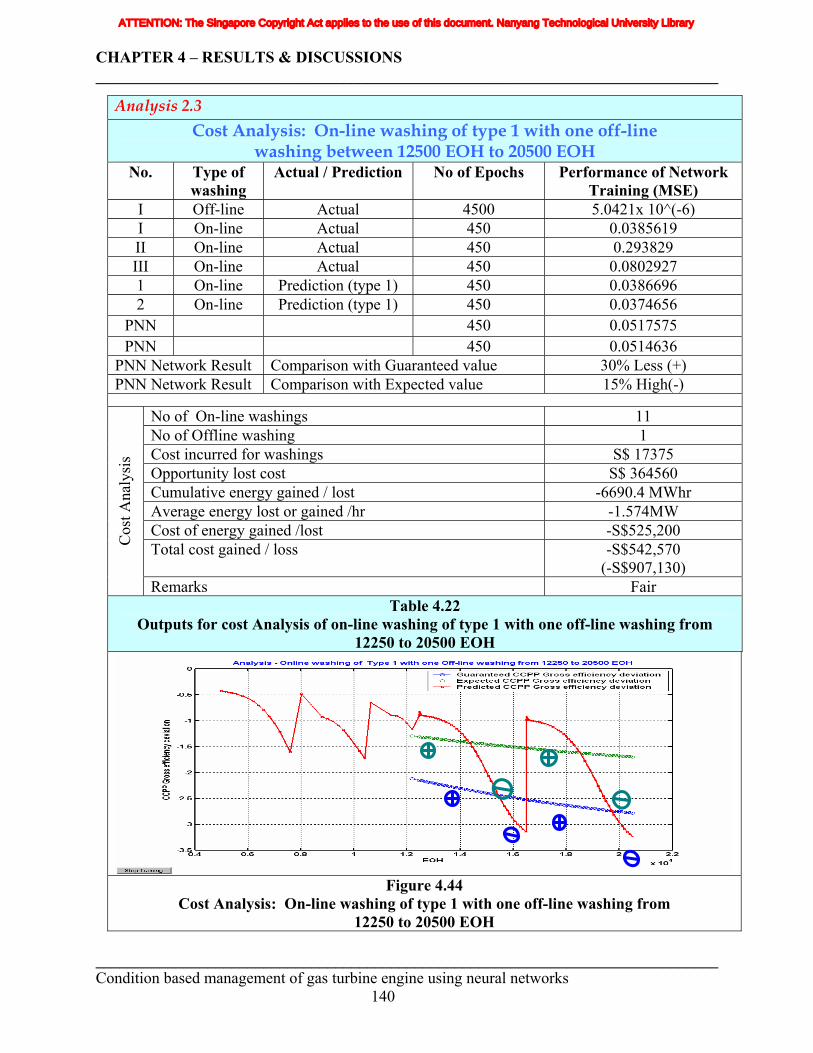
CHAPTER 4 – RESULTS & DISCUSSIONS ______________________________________________________________________________
Analysis 2.3 Cost Analysis: On-line washing of type 1 with one off-line
washing between 12500 EOH to 20500 EOH No. Type of
washing Actual / Prediction No of Epochs Performance of Network
Training (MSE) I Off-line Actual 4500 5.0421x 10^(-6) I On-line Actual 450 0.0385619 II On-line Actual 450 0.293829 III On-line Actual 450 0.0802927 1 On-line Prediction (type 1) 450 0.0386696 2 On-line Prediction (type 1) 450 0.0374656
PNN 450 0.0517575 PNN 450 0.0514636
PNN Network Result Comparison with Guaranteed value 30% Less (+) PNN Network Result Comparison with Expected value 15% High(-)
No of On-line washings 11 No of Offline washing 1 Cost incurred for washings S$ 17375 Opportunity lost cost S$ 364560 Cumulative energy gained / lost -6690.4 MWhr Average energy lost or gained /hr -1.574MW Cost of energy gained /lost -S$525,200 Total cost gained / loss -S$542,570
(-S$907,130)
Cos
t Ana
lysi
s
Remarks Fair Table 4.22
Outputs for cost Analysis of on-line washing of type 1 with one off-line washing from 12250 to 20500 EOH
Figure 4.44
Cost Analysis: On-line washing of type 1 with one off-line washing from 12250 to 20500 EOH
______________________________________________________________________________ Condition based management of gas turbine engine using neural networks 140
ATTENTION: The Singapore Copyright Act applies to the use of this document. Nanyang Technological University Library
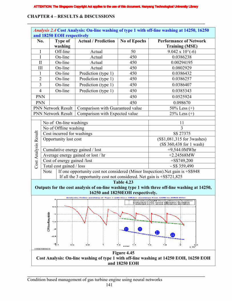
CHAPTER 4 – RESULTS & DISCUSSIONS ______________________________________________________________________________
Analysis 2.4 Cost Analysis: On-line washing of type 1 with off-line washing at 14250, 16250 and 18250 EOH respectively
No. Type of washing
Actual / Prediction No of Epochs Performance of Network Training (MSE)
I Off-line Actual 50 9.042 x 10^(-6) I On-line Actual 450 0.0386238 II On-line Actual 450 0.00294195 III On-line Actual 450 0.0802929 1 On-line Prediction (type 1) 450 0.0386432 2 On-line Prediction (type 1) 450 0.0386257 3 On-line Prediction (type 1) 450 0.0386407 4 On-line Prediction (type 1) 450 0.0385343
PNN 450 0.0525924 PNN 450 0.098670
PNN Network Result Comparison with Guaranteed value 50% Less (+) PNN Network Result Comparison with Expected value 25% Less (+)
No of On-line washings 11 No of Offline washing 3 Cost incurred for washings S$ 27375 Opportunity lost cost (S$1,081,315 for 3washes)
(S$ 360,438 for 1 wash) Cumulative energy gained / lost +9,544.0MWhr Average energy gained or lost / hr +2.24568MW Cost of energy gained /lost +S$749,200 Total cost gained / loss - S$ 359,490 C
ost A
naly
sis R
esul
t
Note If all the 3 opportunity cost not considered. Net gain is +S$721,825
Table 4.23 Outputs for the cost analysis of on-line washing type 1 with three off-line washing at 14250,
16250 and 18250EOH respectively.
Figure 4.45
Cost Analysis: On-line washing of type 1 with off-line washing at 14250 EOH, 16250 EOH and 18250 EOH
If one opportunity cost not considered (Minor Inspection).Net gain is +S$948
______________________________________________________________________________ Condition based management of gas turbine engine using neural networks 141
ATTENTION: The Singapore Copyright Act applies to the use of this document. Nanyang Technological University Library
CHAPTER 4 – RESULTS & DISCUSSIONS ______________________________________________________________________________
______________________________________________________________________________ Condition based management of gas turbine engine using neural networks 142
The graphical output of this model is shown Figure 4.44. The cost analysis part of the
model shows that with opportunity lost consideration, there is net loss of around S$ 907,130 per
year. It is recommended by the gas turbine supplier that for every 4000 EOH, the gas turbine hot
sections to be inspected compulsorily. Normally the offline washing and compressor blade
cleaning activities are done during this period. So by deleting the opportunity lost cost, the net
loss is around S$542,570. (Approximately equal to 1.08% of the annual profit of gained by
running this gas turbine). The net loss can be further minimized by using type 2 and type 3 on-
line washing intervals.
4.2.2.4 Cost analysis of on-line washing type 1 with three off-line washing at 14250,
16250, 18250 EOH respectively
Normally two minor inspections are performed every year. In this scenario one additional
off-line washing has been performed between this two minor inspection and their effects are
analyzed in annual basis. The CCPP gross efficiency deviation based on OEM corrections and
corresponding washing details from the tenth column of the table 4.15 have been given as input
to the hybrid neural network model based on prestd technique. The outputs of the model are
shown in Analysis 2.4.
Table 4.23 in the analysis 2.4 gives the statistical output data of the model. The graphical
output of the thermal analysis using this model has been shown in Figure 4.45. It shows that the
CCPP gross efficiency degradation is about 50% lesser (better) than the guaranteed value and
25% lesser (better) than the expected degradation value.
The cost analysis part of the model shows as follows,
Net loss of around S$ 359,490 per year. (All the three off-line washing plus
compressor IGV blade cleaning opportunity cost lost are included).
Net loss of around S$949 per year. (The two off-line washing plus compressor IGV
blade cleaning opportunity cost lost are included and remaining one off-line washing
plus IGV blade cleaning opportunity is covered under the minor inspection).
Net gain of around S$ 721,825 per year. (All the three off-line washing plus
compressor IGV blade cleaning opportunity cost lost are not included).
ATTENTION: The Singapore Copyright Act applies to the use of this document. Nanyang Technological University Library
CHAPTER 5 – CONCLUSION AND RECOMMENDATIONS ______________________________________________________________________________
5.1 Conclusion The evaluation of different variants of the steady state network model revealed that the
hybrid neural network model has the ability to replicate the complicate gas turbine compressor
degradation with great accuracy. The accuracy largely depends on the extended and variety of
training data available, the type of pre-processing carried out, the choice of training method and
the transfer function used.
The model possesses good flexibility in both training and prediction. This leads to the
high adaptive nature of the model to the real system. The degradation rates vary and very
specific to each plant depending on their site location, surrounding environment, climatic
conditions and plant layout. The adaptive nature of the neural network model allows the user to
tune the model specific to that engine. The decisions are taken based on the history of the engine
and not from the standard recommendations. The training of the model is very easy, since it
does not require any sophisticated geometrical details of the gas turbine internals. It is more user
friendly and fast enough to be used.
The gas turbine GHI parameters degradation determination using OEM and STD
corrections for the long term trending shows that degradation curve has the same profile with
minor deviations in its value. This proves that the developed model is a good tool to asses the
health of gas turbine compressor of both constant and variable speed types. The accuracy level
for the constant speed gas turbines other than V94.3A type would be up to only first order level,
since the other types need their individual OEM corrections.
The cost analysis of the model explains that even 1MWhr of energy loss per hour due to
improper washing schedule leads to approximately half million dollar loss per annum.
All the above concludes that the developed hybrid neural network model is user friendly
and very effective tool for analyzing the gas turbine compressor health monitoring.
5.2 Recommendations on scheduling of compressor washing: The main findings and recommendations related to the hybrid neural network model
developed for assessing the gas turbine compressor health are as follows:
Currently the on-line washings are done as preventive maintenance on monthly basis. (ie
about every 720 EOH). Instead if the interval of on-line washing is decreased to 600 EOH the
______________________________________________________________________________ Condition based management of gas turbine engine using neural networks 143
ATTENTION: The Singapore Copyright Act applies to the use of this document. Nanyang Technological University Library
CHAPTER 5 – CONCLUSION AND RECOMMENDATIONS ______________________________________________________________________________
energy lost could be reduced from 5175MWhr to 3550MWhr for a period of 4000 EOH. It could
be reduced further by decreasing the on-line washing interval to 470EOH.
But frequent on-line washing using chemicals would have adverse effect on the blade
coating and blade cooling holes blockage. To overcome the above problem, more frequent on-
line washing could be done by using de-mineralized water. The profiles of the first stage vane
play critical roles in deciding the airflow rate through the gas turbine compressor and it tends to
be most heavily fouled. These deposits become more difficult to remove if left untreated and the
aging process bonds them more firmly to the airfoil. The frequent on-line washing is most
effective in removing the deposits on the first two or three compressor stages and significantly
decreases the fouling rate and maintains good performance level. Its effects can be analyzed
using the developed hybrid neural network model.
Normally the off-line washing plus compressor IGV blade cleaning are done during the
minor outages. (ie every 4000 EOH) . If one additional off-line washing plus compressor blade
cleaning is performed in between this period, it results in good amount of energy saving
(3960MWhr per 4000EOH). But the lost of power generation opportunity cost overrides the
energy saved.
The power selling prices are very low during week ends and holidays. If the two and half
days required for the washing is covered in one of these days it will leads to good amount
of energy and cost saving.
The gas turbine availability is around 92% (336days) per annum and planned minor
inspection time is about 3% (11 days) per annum. The remaining (5%) 18 days are due to
the unplanned breakdowns of the engine and auxiliary system. If 2.5 days from this
unplanned breakdown slot is utilized for doing the compressor off-line washing it will
lead to savings of about 8000MWhr per year.
The compressor off-line washing and IGV blade cleaning are combined during minor
outage times. These two activities together take 2.5 days. The time duration of the compressor
IGV blade cleaning and off-line washing are 2.25 days and two hours respectively. Even though
the off-line washing needs only 2 hours, it requires gas turbine to be shutdown condition. The
shutting down plus starting of the gas turbine and steam turbine takes roughly four hours. So far
______________________________________________________________________________ Condition based management of gas turbine engine using neural networks 144
ATTENTION: The Singapore Copyright Act applies to the use of this document. Nanyang Technological University Library

CHAPTER 5 – CONCLUSION AND RECOMMENDATIONS ______________________________________________________________________________
the effect of the off-line washing alone is not tested at the site. At least one trial attempt could be
done and the effect of off-line washing alone can be analyzed using the hybrid neural model
developed and based on the result, further decision could be made.
5.3 Challenges and Recommendations for Future Work
5.3.1 Extension to the present work In this research work, main focus has been given to asses the effect of compressor fouling
on the gas turbine performance by using the hybrid neural network model and recommendations
are made to reduce the losses by proper planning of washing schedules. Further investigation
should be devoted to the application of the developed hybrid neural network model in the
following areas.
Assessments of the recoverable and non-recoverable losses of the gas turbine based on
the fouling of its combustor and turbine.
The effects of fouling on the HRSG tube’s internal surface, external surface, passing
valves and steam traps could be assessed and recommendation regarding acid washing
frequency of HRSG tubes internal surfaces, air jet cleaning of the HRSG tube’s external
surfaces, renewal of passing valves and steam traps could be made.
Further works to be done in order to assess the fouling effects on the steam turbine
performance and recommendations like silica washing of turbine could also be done.
The hybrid neural network model could also used to investigate and study the following
fouling inter effects in a CCPP and Cogeneration plant
a. The effects of the gas turbine fouling on the HRSG and the steam turbine
performance.
b. The effects of the HRSG fouling on the gas turbine and steam turbine
performance.
At least 3 years of operating data are required for training the developed model for all
the above cases, but it is worth to proceed with the further research work in the above areas
considering the 25 years of expected life from the CCPP.
______________________________________________________________________________ Condition based management of gas turbine engine using neural networks 145
ATTENTION: The Singapore Copyright Act applies to the use of this document. Nanyang Technological University Library
CHAPTER 5 – CONCLUSION AND RECOMMENDATIONS ______________________________________________________________________________
______________________________________________________________________________ Condition based management of gas turbine engine using neural networks 146
5.3.2 Improvements to the present work: Neural network modeling is an empirical modeling. The result from this model depends
on the data used for training it. So the training data should be representative of what an actual
engine will produce. The present hybrid neural network model developed uses the base line
reference data taken from the PAC test result. This PAC test is performed for 60%, 85%, 93%
and 100% loads only, so the curve fitting technique has been used to derive the GHI values for
the intermediate load values. If the data from the gas turbine simulator are used for generating
this intermediate load values then the accuracy of this model would be further improved.
The thermo-economical analysis of the currently developed model has been done based
on the average power generation of the unit, even though in real application it is fluctuating
depending on the grid requirements and market bidding. Normally the market bidding is done
every half an hour, it is very fluctuating due to the sudden raise in demand (other machines
tripping), peak demand periods ( Day times when the industries need more power) and off peak
periods ( like Sundays and public holidays). The SIMULINK software has got good
compatibility with neural networks, so it could be used to generate output wave forms
representing the fluctuating nature of cost and inputted to the developed hybrid neural network
model. The outputs from this model would be useful the power plant operators in the real
applications.
ATTENTION: The Singapore Copyright Act applies to the use of this document. Nanyang Technological University Library
REFERENCES _____________________________________________________________________________________________
1. Bernard Becker (2002), Robust gas turbine design,
ASME Turbo Expo 2002, Paper No.2002-GT-30159.
2. Bhargava Rakesh(1992), On-site performance evaluation of critical components in a
cogeneration plant, ASME COGEN-TURBO 1992 – IGTI - Vol 7.
3. British standard (1989), Specification for gas turbine acceptance tests – BS 3135, ISO2314,
UK, British standards.
4. Brooks F.J., GE Turbine Performance Characteristics, GE Reference Library, publication
GER 3567H.
5. Cohen.H , Rogers.G.F.C . & Saravanamutto.H.I.H. (1982),Gas turbine theory , Essex, U.K,
Longman Group Limited.
6. Cornforth. J.R (1992), Combustion engineering and gas utilization, London, British gas
E & FN SPON.
7. Giampaolo Tony(1997), The gas turbine handbook- principles and practices, Lilburn, GA,
The fairmont press, Inc.
8. Gregory J.Kacprzynski & Daniel E.Caguiat (2001). A prognostic modeling approach for
predicting recurring maintenance for shipboard propulsion system,
ASME Paper No. 2001-GT-0218.
9. Hanselman Duane& Littlefield Bruce.(2001). Mastering of Matlab 6.0,
New Jersey, Prentice-Hall.
10. Horlock. J.H(1992), Combined power plants- including combined cycle gas turbines
(CCGT), England/USA/Seoul/Tokyo, Pergamon Press Ltd.
11. IGTI (1996), Home study of gas turbine applications and economics, Atlanta, ASME
International Gas Turbine Institute.
Condition based management of gas turbine engine using neural networks
147
ATTENTION: The Singapore Copyright Act applies to the use of this document. Nanyang Technological University Library
REFERENCES _____________________________________________________________________________________________
12. Irvine.F. Thomas, Jr & Peter E.Liley (1984), Steam and gas tables with computer
equations, Londan, Acadamic Press, Inc Ltd.
13. Jean-Pierre Stalder (1998). Gas turbine compressor washing state of art – field experiences.
ASME Paper No 98-GT-420.
14. Kenneth McGarry, Stefan Wermter and John Maclntyre(1999) , Hybrid neural systems: From
simple coupling to fully integrated neural networks, Sunderland, School of computing,
University of Sunderland.
15. Leusden, Sorgenfrey and Lutz Dummel (2003), Performance benefits using Siemens
Advanced compressor-cleaning system, ASME Turbo Expo Paper No. 2003-GT-38184.
16. Lorenzo Dambrosio, Marco Bombo, Sergio M.Camporeale and Bernardo Fortunato (2002),
Feedforward neural network based diagnostic tool for gas turbine power plant, ASME Turbo
Expo Paper No-2002-GT-30019.
17. Math Works Inc, (2000a), Matlab 6.0 User's guide, Natick, MA.
18. Mathioudakis.K (2002), Gas turbine parameters corrections including operation with water
injection, ASME Turbo Expo Paper No. GT-2002-30466.
19. Michael J. Roemer, Gregory J. Kacprzynski, Michael Gumina, Daniel E. Caguait, Thomas
R. Galie and Jack J. McGroarty (2001), A prognostic modeling approach for predicting
recurring maintenance for shipboard propulsion system, ASME Turbo Expo Paper No –
2001-GT-0218.
20. Neophytos Chiras, Ceriv Evans and David Rees (2002), Non linear Gas turbine modeling
using Feedforward Neural Networks, ASME Turbo Expo Paper No. GT-2002-30035.
21. Robert J. Schalkoff (1997), Artificial Neural Networks, Singapore, McGraw –Hill
Companies.
Condition based management of gas turbine engine using neural networks
148
ATTENTION: The Singapore Copyright Act applies to the use of this document. Nanyang Technological University Library
REFERENCES _____________________________________________________________________________________________
Condition based management of gas turbine engine using neural networks
149
22. Romessis.C , Stamatis.A and Mathioudakis.K (2001). A parametric investigation of the
diagnostic ability of probabilistic neural network on turbofan engines,
ASME Paper No. 2001-GT-0011.
23. Sawyer W. John (1985), Sawyer's gas turbine engineering handbook –Volume I, II & III,
Norwalk, Connecticut, Turbomachinery International publications.
24. Singh, Ranjeet (2001), Application of Steady state data in aircraft engine modeling,
monitoring and diagnosis, final year project report, School of Mechanical and Production
Engineering, Nanyang Technological University, Singapore.
25. Sun Bon and Zhang Jin (2000), An Investigation of Artificial Neural Network (ANN) in
quantitative fault diagnosis for turbo engine, International Gas turbine Institute -
Turbo Expo Paper No. 2000-GT-32.
26. Siemens (2001), Plant Course – Overview to design and operation of the Siemens combined
cycle power plant (CCPP), Germany, Siemens.
27. Philp P. Wash and Paul Fletcher(2004), Gas turbine performance, New jersey/ USA,
Blackwell science Ltd and ASME.
28. Wolfgang Menapace, Matthias Frankle and Bert Rukes(2003), Combined cycle power plant
concepts meeting the demand for operational flexibility, Siemens AG Power Generation,
POWER-GEN ASIA -2003 Paper No. ID 203.
ATTENTION: The Singapore Copyright Act applies to the use of this document. Nanyang Technological University Library

Appendix A
ATTENTION: The Singapore Copyright Act applies to the use of this document. Nanyang Technological University Library
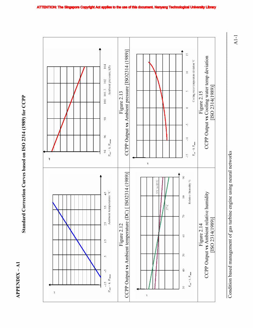
APP
EN
DIX
– A
1 St
anda
rd C
orre
ctio
n C
urve
s bas
ed o
n IS
O 2
314
(198
9) fo
r C
CPP
Figu
re 2
.12
CC
PP O
utpu
t vs A
mbi
ent t
empe
ratu
re (D
C) [
ISO
2314
(198
9)]
Figu
re 2
.13
CC
PP O
utpu
t vs A
mbi
ent p
ress
ure
[ISO
2314
(198
9)]
Figu
re 2
.14
CC
PP O
utpu
t vs A
mbi
ent r
elat
ive
hum
idity
[I
SO 2
314(
1989
)]
Figu
re 2
.15
CC
PP O
utpu
t vs C
oolin
g w
ater
tem
p de
viat
ion
[ISO
231
4(19
89)]
____
____
____
____
____
____
____
____
____
____
____
____
____
____
____
____
____
____
____
____
____
____
____
____
____
____
___
Con
ditio
n ba
sed
man
agem
ent o
f gas
turb
ine
engi
ne u
sing
neu
ral n
etw
orks
A1-
1
ATTENTION: The Singapore Copyright Act applies to the use of this document. Nanyang Technological University Library
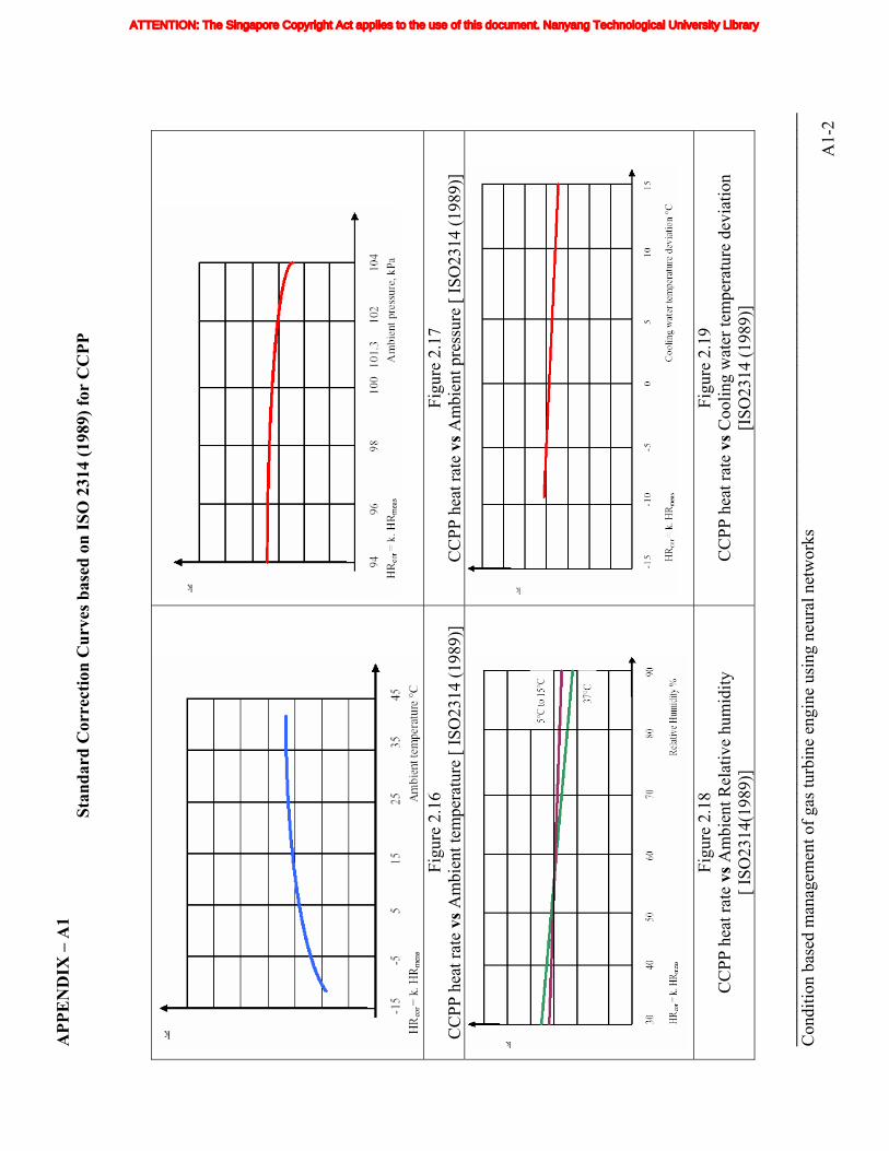
APP
EN
DIX
– A
1 St
anda
rd C
orre
ctio
n C
urve
s bas
ed o
n IS
O 2
314
(198
9) fo
r C
CPP
Figu
re 2
.16
CC
PP h
eat r
ate
vs A
mbi
ent t
empe
ratu
re [
ISO
2314
(198
9)]
Figu
re 2
.17
CC
PP h
eat r
ate
vs A
mbi
ent p
ress
ure
[ ISO
2314
(198
9)]
Figu
re 2
.18
CC
PP h
eat r
ate
vs A
mbi
ent R
elat
ive
hum
idity
[ I
SO23
14(1
989)
]
Figu
re 2
.19
CC
PP h
eat r
ate
vs C
oolin
g w
ater
tem
pera
ture
dev
iatio
n
[ISO
2314
(198
9)]
____
____
____
____
____
____
____
____
____
____
____
____
____
____
____
____
____
____
____
____
____
____
____
____
____
____
___
Con
ditio
n ba
sed
man
agem
ent o
f gas
turb
ine
engi
ne u
sing
neu
ral n
etw
orks
A1-
2
ATTENTION: The Singapore Copyright Act applies to the use of this document. Nanyang Technological University Library
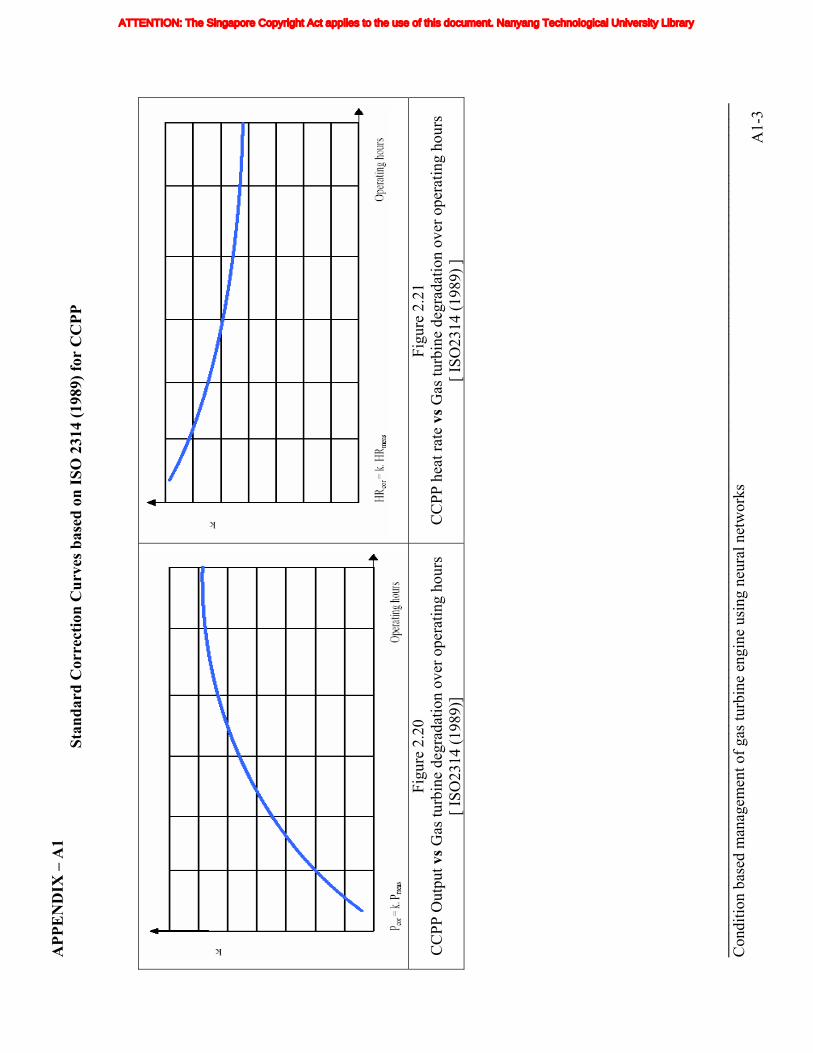
APP
EN
DIX
– A
1 St
anda
rd C
orre
ctio
n C
urve
s bas
ed o
n IS
O 2
314
(198
9) fo
r C
CPP
____
____
____
____
____
____
____
____
____
____
____
____
____
____
____
____
____
____
____
____
____
____
____
____
____
____
___
Con
ditio
n ba
sed
man
agem
ent o
f gas
turb
ine
engi
ne u
sing
neu
ral n
etw
orks
A1-
3
Figu
re 2
.20
CC
PP O
utpu
t vs G
as tu
rbin
e de
grad
atio
n ov
er o
pera
ting
hour
s [ I
SO23
14 (1
989)
]
Figu
re 2
.21
CC
PP h
eat r
ate
vs G
as tu
rbin
e de
grad
atio
n ov
er o
pera
ting
hour
s [ I
SO23
14 (1
989)
]
ATTENTION: The Singapore Copyright Act applies to the use of this document. Nanyang Technological University Library
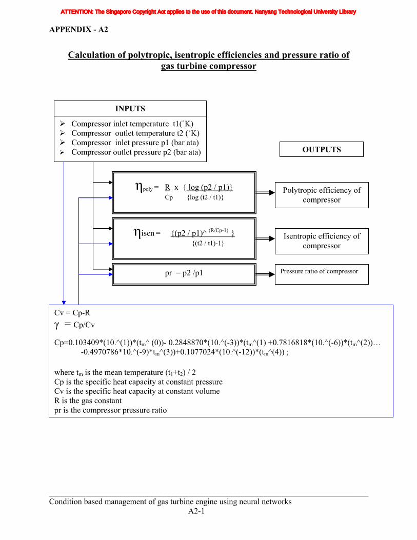
APPENDIX - A2
Calculation of polytropic, isentropic efficiencies and pressure ratio of gas turbine compressor
OUTPUTS
INPUTS
Pressure ratio of compressor
Isentropic efficiency of compressor
Polytropic efficiency of compressor
Cv = Cp-R γ = Cp/Cv Cp=0.103409*(10.^(1))*(tm^ (0))- 0.2848870*(10.^(-3))*(tm^(1) +0.7816818*(10.^(-6))*(tm^(2))… -0.4970786*10.^(-9)*tm^(3))+0.1077024*(10.^(-12))*(tm^(4)) ; where tm is the mean temperature (t1+t2) / 2 Cp is the specific heat capacity at constant pressure Cv is the specific heat capacity at constant volume R is the gas constant pr is the compressor pressure ratio
pr = p2 /p1
ηisen = {(p2 / p1)^ (R/Cp-1) } {(t2 / t1)-1}
ηpoly = R x { log (p2 / p1)} Cp {log (t2 / t1)}
Compressor inlet temperature t1(˚K) Compressor outlet temperature t2 (˚K) Compressor inlet pressure p1 (bar ata) Compressor outlet pressure p2 (bar ata)
______________________________________________________________________________ Condition based management of gas turbine engine using neural networks A2-1
ATTENTION: The Singapore Copyright Act applies to the use of this document. Nanyang Technological University Library
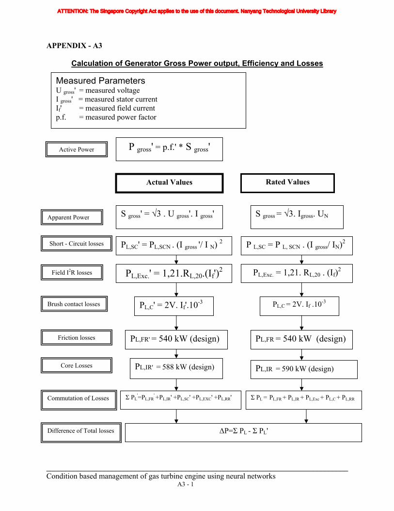
APPENDIX - A3
Co
Calculation of Generator Gross Power output, Efficiency and Losses
Measured Parameters U gross' = measured voltage I gross' = measured stator current If' = measured field current p.f. = measured power factor
P gross' = p.f.' * S gross' r
__
Ap
Sh
F
Bru
Co
Dif
ATTENTION: The Singapore Copyright Act applies to the use of this document. Nanyang Technological University Library
Active Powe
ndition based management of gas turbine engine using neural networks A3 - 1
Actual Values Rated Values
____________________________________________________________________________
P L,SC = P L, SCN . (I gross/ IN)2 PL,SC' = PL,SCN . (I gross '/ I N) 2
S gross = √3. Igross. UN
S gross' = √3 . U gross'. I gross'
parent Power
ort - Circuit losses
PL,Exc.' = 1,21.RL,20.(If')2 PL,Exc. = 1,21. RL,20 . (If)2 ield I2R losses
PL,C' = 2V. If'.10-3 PL,C = 2V. If .10-3 sh contact losses
PL,FR' = 540 kW (design) PL,FR = 540 kW (design) Friction losses
PL,IR' = 588 kW (design) Core Losses PL,IR = 590 kW (design)
Σ PL'=PL,FR
' +PL,IR' +PL,SC' +PL,EXC' +PL,RR'
Σ PL = PL,FR + PL,IR + PL,Exc + PL,C + PL,RR mmutation of Losses
∆P=Σ PL - Σ PL' ference of Total losses
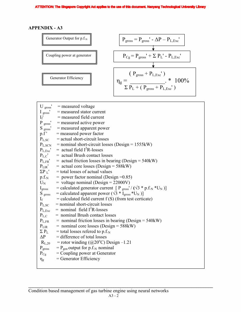
APPENDIX - A3
______________________________________________________________________________ Condition based management of gas turbine engine using neural networks A3 - 2
Generator Efficiency
Generator Output for p.f.N
( Pgross + PL,Exc' ) ηg = ___________. * 100% Σ PL + ( Pgross + PL,Exc' )
PCg = Pgross' + Σ PL' - PL,Exc' Coupling power at generator
Pgross = Pgross' - ∆P – PL,Exc'
U gross' = measured voltage I gross' = measured stator current If' = measured field current P gross' = measured active power S gross' = measured apparent power p.f ' = measured power factor PL,SC = actual short-circuit losses PL,SCN = nominal short-circuit losses (Design = 1555kW) PL,Exc' = actual field I2R-losses PL,C' = actual Brush contact losses PL,FR' = actual friction losses in bearing (Design = 540kW) PLIR' = actual core losses (Design = 588kW) ΣP L' = total losses of actual values p.f.N = power factor nominal (Design =0.85) UN = voltage nominal (Design = 22000V) Igross = calculated generator current [ P gross' / (√3 * p.f.N *UN )] S gross = calculated apparent power (√3 * Igross *UN )] If = calculated field current f (S) (from test certicate) PL,SC = nominal short-circuit losses PL,Exc = nominal field I2R-losses PL,C = nominal Brush contact losses PL,FR = nominal friction losses in bearing (Design = 540kW) PLIR = nominal core losses (Design = 588kW) Σ PL = total losses refered to p.f.N ∆P = difference of total losses RL,20 = rotor winding (@20oC) Design –1.21 Pgross = Pgen output for p.f.N nominal PCg = Coupling power at Generator ηg = Generator Efficiency
ATTENTION: The Singapore Copyright Act applies to the use of this document. Nanyang Technological University Library
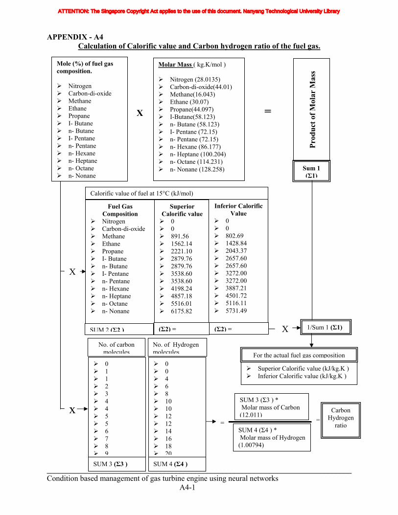
APPENDIX - A4
Calculation of Calorific value and Carbon hydrogen ratio of the fuel gas.
Mole (%) of fuel gas composition.
Nitrogen Carbon-di-oxide Methane Ethane Propane I- Butane n- Butane I- Pentane n- Pentane n- Hexane n- Heptane n- Octane n- Nonane
Molar Mass ( kg.K/mol )
Nitrogen (28.0135) Carbon-di-oxide(44.01) Methane(16.043) Ethane (30.07) Propane(44.097) I-Butane(58.123) n- Butane (58.123) I- Pentane (72.15) n- Pentane (72.15) n- Hexane (86.177) n- Heptane (100.204) n- Octane (114.231) n- Nonane (128.258)
Pr
oduc
t of M
olar
Mas
s
= X
Sum 1 (Σ1)
Calorific value of fuel at 15°C (kJ/mol)
Inferior Calorific Value
0 0 802.69 1428.84 2043.37 2657.60 2657.60 3272.00 3272.00 3887.21 4501.72 5116.11 5731.49
Fuel Gas Composition
Nitrogen Carbon-di-oxide Methane Ethane Propane I- Butane n- Butane I- Pentane n- Pentane n- Hexane n- Heptane n- Octane n- Nonane
Superior Calorific value 0 0 891.56 1562.14 2221.10 2879.76 2879.76 3538.60 3538.60 4198.24 4857.18 5516.01 6175.82
X
1/Sum 1 (Σ1) X (Σ2) = (Σ2) =SUM 2 (Σ2 )
No. of carbon molecules
No. of Hydrogen molecules For the actual fuel gas composition
______________________________________________________________________________ Condition based management of gas turbine engine using neural networks A4-1
0 0 4 6 8 10 10 12 12 14 16 18
20SUM 4 (Σ4 )
0 1 1 2 3 4 4 5 5 6 7 8
9SUM 3 (Σ3 )
Superior Calorific value (kJ/kg.K ) Inferior Calorific value (kJ/kg.K )
SUM 3 (Σ3 ) * Molar mass of Carbon (12.011)x Carbon
Hydrogen ratio
= =SUM 4 (Σ4 ) * Molar mass of Hydrogen (1.00794)
ATTENTION: The Singapore Copyright Act applies to the use of this document. Nanyang Technological University Library
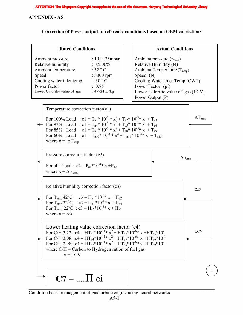
APPENDIX - A5
Correction of Power output to reference conditions based on OEM corrections
______________________________________________________________________________ Condition based management of gas turbine engine using neural networks A5-1
C7 = I =1 to 4 Π ci
1
LCV
Ư
∆pamp
∆Tamp
Lower heating value correction factor (c4) For C/H 3.22: c4 = HTa1*10-11* x2 + HTa2*10-6* x +HTa3*10-1 For C/H 3.08: c4 = HTa4*10-11* x2 + HTa5*10-6* x +HTa6*10-1 For C/H 2.98: c4 = HTa7*10-11* x2 + HTa8*10-6* x +HTa9*10-1 where C/H = Carbon to Hydrogen ration of fuel gas x = LCV
Relative humidity correction factor(c3) For Tamp 42oC : c3 = Ha1*10-4* x + Ha2 For Tamp 32oC : c3 = Ha3*10-4* x + Ha4 For Tamp 22oC : c3 = Ha5*10-4* x + Ha6 where x = Ư
Pressure correction factor (c2) For all Load : c2 = Pa1*10-4* x +Pa2 where x = ∆p amb
Temperature correction factor(c1) For 100% Load : c1 = Ta1* 10-5 * x2 + Ta2* 10-3* x + Ta3 For 93% Load : c1 = Ta4* 10-5 * x2 + Ta5* 10-3* x + Ta6 For 85% Load : c1 = Ta7* 10-5 * x2 + Ta8* 10-3* x + Ta9 For 60% Load : c1 = Ta10* 10-5 * x2 + Ta11* 10-3* x + Ta13 where x = ∆Tamp
Actual Conditions Ambient pressure (pamp) Relative Humidity (Ø) Ambient Temperature (Tamp) Speed (N) Cooling Water Inlet Temp (CWT) Power Factor (pf) Lower Calorific value of gas (LCV) Power Output (P)
Rated Conditions Ambient pressure : 1013.25mbar Relative humidity : 85.00% Ambient temperature : 32 º C Speed : 3000 rpm Cooling water inlet temp : 30 º C Power factor : 0.85 Lower Calorific value of gas : 45724 kJ/kg
ATTENTION: The Singapore Copyright Act applies to the use of this document. Nanyang Technological University Library
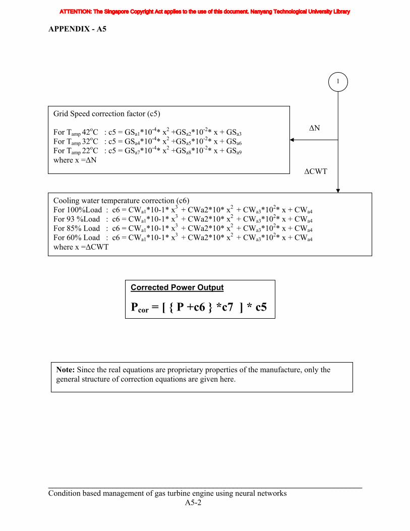
APPENDIX - A5
______________________________________________________________________________ Condition based management of gas turbine engine using neural networks A5-2
Corrected Power Output
Pcor = [ { P +c6 } *c7 ] * c5
∆CWT
∆N
1
Cooling water temperature correction (c6) For 100%Load : c6 = CWa1*10-1* x3 + CWa2*10* x2 + CWa3*102* x + CWa4 For 93 %Load : c6 = CWa1*10-1* x3 + CWa2*10* x2 + CWa3*102* x + CWa4 For 85% Load : c6 = CWa1*10-1* x3 + CWa2*10* x2 + CWa3*102* x + CWa4 For 60% Load : c6 = CWa1*10-1* x3 + CWa2*10* x2 + CWa3*102* x + CWa4 where x =∆CWT
Grid Speed correction factor (c5) For Tamp 42oC : c5 = GSa1*10-4* x2 +GSa2*10-2* x + GSa3 For Tamp 32oC : c5 = GSa4*10-4* x2 +GSa5*10-2* x + GSa6 For Tamp 22oC : c5 = GSa7*10-4* x2 +GSa8*10-2* x + GSa9 where x =∆N
Note: Since the real equations are proprietary properties of the manufacture, only the general structure of correction equations are given here.
ATTENTION: The Singapore Copyright Act applies to the use of this document. Nanyang Technological University Library
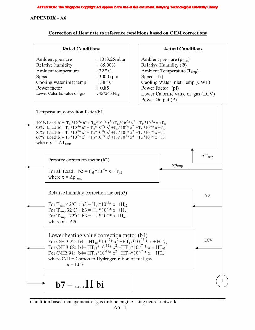
APPENDIX - A6
Correction of Heat rate to reference conditions based on OEM corrections
b7 = I =1 to 4 Π bi 1
LCV
Ư
∆pamp
∆Tamp
Lower heating value correction factor (b4) For C/H 3.22: b4 = HTa1*10-12* x2 +HTa2*10-07 * x + HTa3 For C/H 3.08: b4= HTa1*10-12* x2 +HTa2*10-07 * x + HTa3 For C/H2.98: b4= HTa1*10-12* x2 +HTa2*10-07 * x + HTa3 where C/H = Carbon to Hydrogen ration of fuel gas x = LCV
Relative humidity correction factor(b3) For Tamp 42oC : b3 = Ha1*10-5* x +Ha2 For Tamp 32oC : b3 = Ha1*10-5* x +Ha2 For Tamp 22oC: b3 = Ha1*10-7* x +Ha2 where x = Ư
Pressure correction factor (b2) For all Load : b2 = Pa1*10-6* x + Pa2 where x = ∆p amb
Temperature correction factor(b1) 100% Load: b1= Ta1*10-8* x4 + Ta2*10-7* x3 +Ta3*10-5* x2 +Ta4*10-5* x +Ta5 93% Load :b1= Ta1*10-8* x4 + Ta2*10-7* x3 +Ta3*10-6* x2 +Ta4*10-4* x +Ta5 85% Load :b1= Ta1*10-9* x4 + Ta2*10-8* x3 +Ta3*10-6* x2 +Ta4*10-4* x +Ta5 60% Load :b1= Ta1*10-9* x4 + Ta2*10-7* x3 +Ta3*10-6* x2 +Ta4*10-4* x +Ta5
where x = ∆Tamp
Actual Conditions Ambient pressure (pamp) Relative Humidity (Ø) Ambient Temperature (Tamp) Speed (N) Cooling Water Inlet Temp (CWT) Power Factor (pf) Lower Calorific value of gas (LCV) Power Output (P)
Rated Conditions Ambient pressure : 1013.25mbar Relative humidity : 85.00% Ambient temperature : 32 º C Speed : 3000 rpm Cooling water inlet temp : 30 º C Power factor : 0.85 Lower Calorific value of gas : 45724 kJ/kg
______________________________________________________________________________ Condition based management of gas turbine engine using neural networks A6 - 1
ATTENTION: The Singapore Copyright Act applies to the use of this document. Nanyang Technological University Library
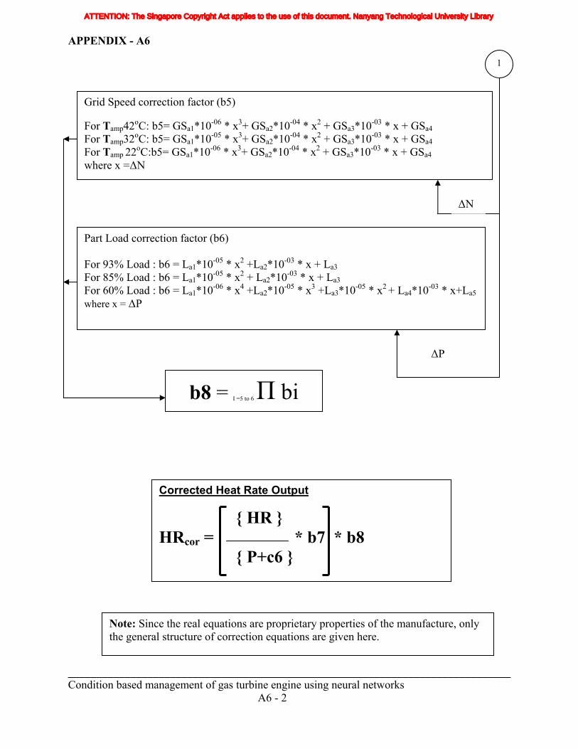
APPENDIX - A6
_______Conditio
Corrected Heat Rate Output
{ HR } HRcor = * b7 * b8
{ P+c6 }
∆P
b8 = I =5 to 6 Π bi
Part Load correction factor (b6) For 93% Load : b6 = La1*10-05 * x2 +La2*10-03 * x + La3 For 85% Load : b6 = La1*10-05 * x2 + La2*10-03 * x + La3 For 60% Load : b6 = La1*10-06 * x4 +La2*10-05 * x3 +La3*10-05 * x2 + La4*10-03 * x+La5 where x = ∆P
∆N
1
Grid Speed correction factor (b5) For Tamp42oC: b5= GSa1*10-06 * x3+ GSa2*10-04 * x2 + GSa3*10-03 * x + GSa4 For Tamp32oC: b5= GSa1*10-05 * x3+ GSa2*10-04 * x2 + GSa3*10-03 * x + GSa4 For Tamp 22oC:b5= GSa1*10-06 * x3+ GSa2*10-04 * x2 + GSa3*10-03 * x + GSa4 where x =∆N
ATTENTION: The Singapore Copyright Act applies to the use of this document. Nanyang Technological University Library
Note: Since the real equations are proprietary properties of the manufacture, onlythe general structure of correction equations are given here.
_______________________________________________________________________ n based management of gas turbine engine using neural networks
A6 - 2
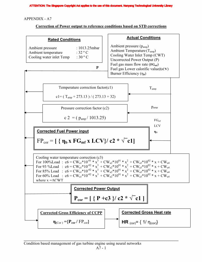
APPENDIX - A7
Correction of Power output to reference conditions based on STD corrections
Corrected Gross Heat rate HR (cor)= { 1/ η(cor)}
Corrected Gross Efficiency of CCPP
η(Cor ) ={Pcor / FPcor}
P
FGmf
LCV
ηB Corrected Fuel Power input
FPcor = [ { ηb x FGmf x LCV}/ c2 * √¯c1]
Corrected Power Output
Pcor = [ { P +c3 }/ c2 * √¯c1 ]
Cooling water temperature correction (c3) For 100%Load : c6 = CWa1*10-01 * x3 + CWa2*1001 * x2 + CWa3*1002 * x + CWa4 For 93 %Load : c6 = CWa1*10-02 * x3 + CWa2*1001 * x2 + CWa3*1002 * x + CWa4 For 85% Load : c6 = CWa1*10-02 * x3 + CWa2*1001 * x2 + CWa3*1002 * x + CWa4 For 60% Load : c6 = CWa1*10-02 * x3 + CWa2*1001 * x2 + CWa3*1002 * x + CWa4 where x =∆CWT
pamp
Tamp
Pressure correction factor (c2)
c 2 = ( pamp / 1013.25)
Temperature correction factor(c1)
c1= ( Tamp + 273.13 ) / ( 273.13 + 32)
Actual Conditions Ambient pressure (pamp) Ambient Temperature (Tamp) Cooling Water Inlet Temp (CWT) Uncorrected Power Output (P) Fuel gas mass flow rate (FGmf) Fuel gas Lower calorific value(LCV) Burner Efficiency (ηB)
Rated Conditions Ambient pressure : 1013.25mbar Ambient temperature : 32 º C Cooling water inlet Temp : 30 º C
______________________________________________________________________________ Condition based management of gas turbine engine using neural networks
A7 - 1
ATTENTION: The Singapore Copyright Act applies to the use of this document. Nanyang Technological University Library
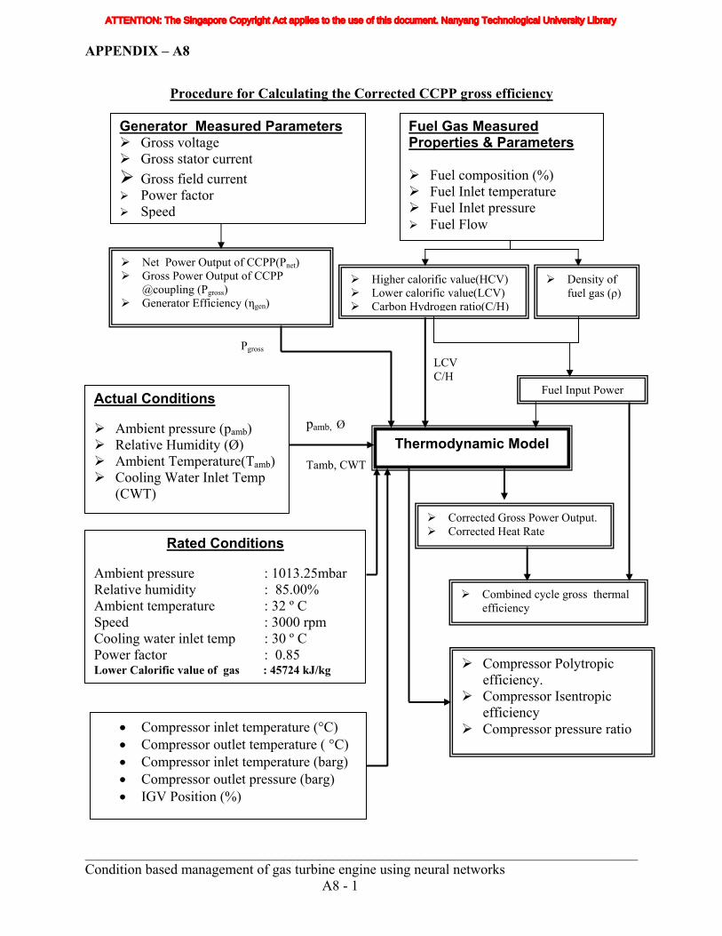
APPENDIX – A8
Procedure for Calculating the Corrected CCPP gross efficiency
Compressor Polytropic efficiency.
Compressor Isentropic efficiency
Compressor pressure ratio • Compressor inlet temperature (°C) • Compressor outlet temperature ( °C) • Compressor inlet temperature (barg) • Compressor outlet pressure (barg) • IGV Position (%)
Combined cycle gross thermal efficiency
Corrected Gross Power Output. Corrected Heat Rate
Rated Conditions Ambient pressure : 1013.25mbar Relative humidity : 85.00% Ambient temperature : 32 º C Speed : 3000 rpm Cooling water inlet temp : 30 º C Power factor : 0.85 Lower Calorific value of gas : 45724 kJ/kg
Thermodynamic Model Tamb, CWT
pamb, Ø
LCV C/H
Pgross
Actual Conditions
Ambient pressure (pamb) Relative Humidity (Ø) Ambient Temperature(Tamb) Cooling Water Inlet Temp
(CWT)
Fuel Input Power
Density of fuel gas (ρ)
Higher calorific value(HCV) Lower calorific value(LCV)
Carbon Hydrogen ratio(C/H)
Fuel Gas Measured Properties & Parameters
Fuel composition (%) Fuel Inlet temperature Fuel Inlet pressure Fuel Flow
Net Power Output of CCPP(Pnet) Gross Power Output of CCPP
@coupling (Pgross) Generator Efficiency (ηgen)
Generator Measured Parameters Gross voltage Gross stator current Gross field current
Power factor Speed
______________________________________________________________________________ Condition based management of gas turbine engine using neural networks A8 - 1
ATTENTION: The Singapore Copyright Act applies to the use of this document. Nanyang Technological University Library
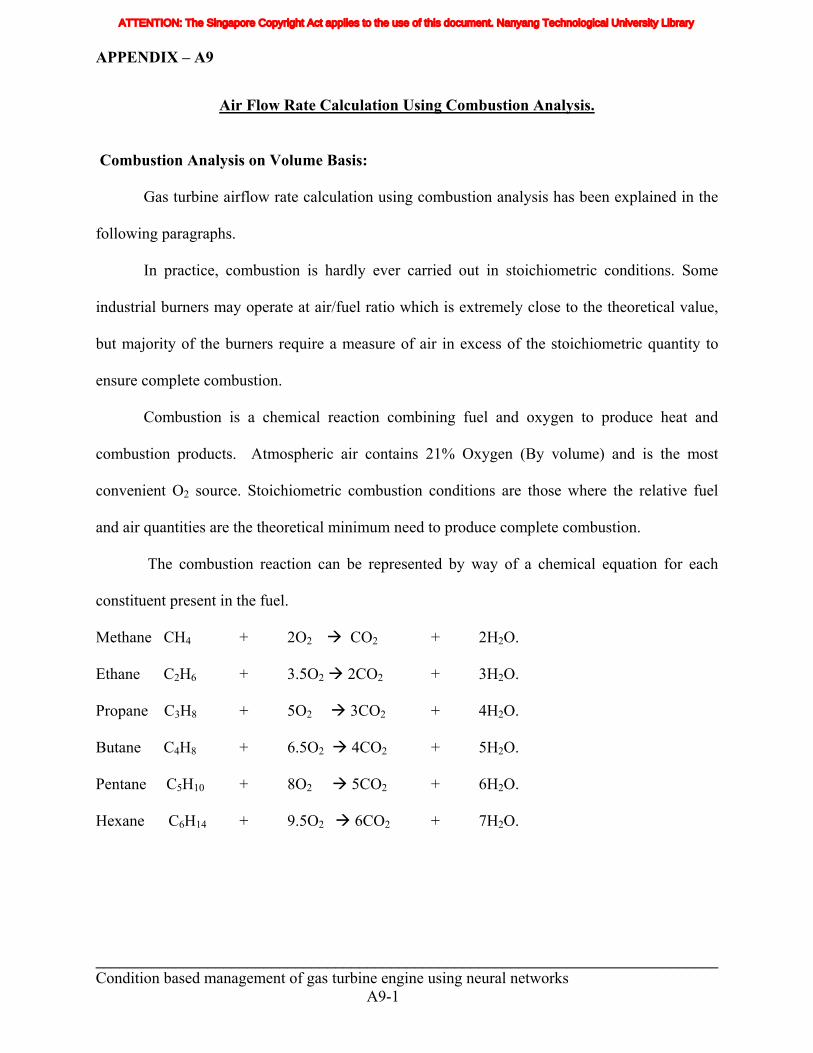
APPENDIX – A9
Air Flow Rate Calculation Using Combustion Analysis.
Combustion Analysis on Volume Basis:
Gas turbine airflow rate calculation using combustion analysis has been explained in the
following paragraphs.
In practice, combustion is hardly ever carried out in stoichiometric conditions. Some
industrial burners may operate at air/fuel ratio which is extremely close to the theoretical value,
but majority of the burners require a measure of air in excess of the stoichiometric quantity to
ensure complete combustion.
Combustion is a chemical reaction combining fuel and oxygen to produce heat and
combustion products. Atmospheric air contains 21% Oxygen (By volume) and is the most
convenient O2 source. Stoichiometric combustion conditions are those where the relative fuel
and air quantities are the theoretical minimum need to produce complete combustion.
The combustion reaction can be represented by way of a chemical equation for each
constituent present in the fuel.
Methane CH4 + 2O2 CO2 + 2H2O.
Ethane C2H6 + 3.5O2 2CO2 + 3H2O.
Propane C3H8 + 5O2 3CO2 + 4H2O.
Butane C4H8 + 6.5O2 4CO2 + 5H2O.
Pentane C5H10 + 8O2 5CO2 + 6H2O.
Hexane C6H14 + 9.5O2 6CO2 + 7H2O.
______________________________________________________________________________ Condition based management of gas turbine engine using neural networks A9-1
ATTENTION: The Singapore Copyright Act applies to the use of this document. Nanyang Technological University Library
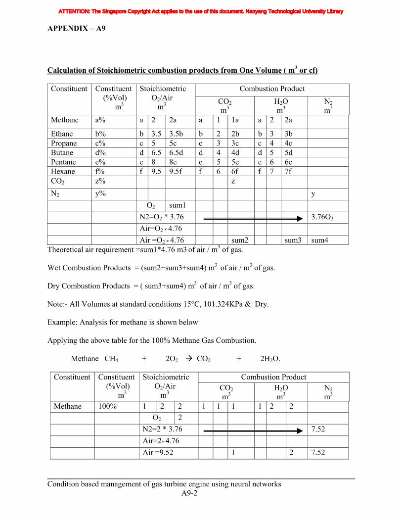
APPENDIX – A9
Calculation of Stoichiometric combustion products from One Volume ( m3 or cf)
Combustion Product Constituent Constituent (%Vol) m3
Stoichiometric O2/Air m3
CO2 m3
H2O m3
N2 m3
Methane a% a 2 2a a 1 1a a 2 2a
Ethane b% b 3.5 3.5b b 2 2b b 3 3b Propane c% c 5 5c c 3 3c c 4 4c Butane d% d 6.5 6.5d d 4 4d d 5 5d Pentane e% e 8 8e e 5 5e e 6 6e Hexane f% f 9.5 9.5f f 6 6f f 7 7f CO2 z% z N2 y% y O2 sum1 N2=O2 * 3.76 3.76O2 Air=O2 * 4.76 Air =O2 * 4.76 sum2 sum3 sum4
Theoretical air requirement =sum1*4.76 m3 of air / m3 of gas.
Wet Combustion Products = (sum2+sum3+sum4) m3 of air / m3 of gas.
Dry Combustion Products = ( sum3+sum4) m3 of air / m3 of gas.
Note:- All Volumes at standard conditions 15°C, 101.324KPa & Dry.
Example: Analysis for methane is shown below
Applying the above table for the 100% Methane Gas Combustion.
Methane CH4 + 2O2 CO2 + 2H2O.
Combustion Product Constituent Constituent (%Vol) m3
Stoichiometric O2/Air m3
CO2 m3
H2O m3
N2 m3
Methane 100% 1 2 2 1 1 1 1 2 2 O2 2 N2=2 * 3.76 7.52 Air=2* 4.76 Air =9.52 1 2 7.52
______________________________________________________________________________ Condition based management of gas turbine engine using neural networks A9-2
ATTENTION: The Singapore Copyright Act applies to the use of this document. Nanyang Technological University Library
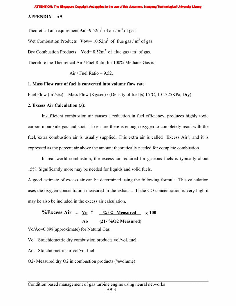
APPENDIX – A9
Theoretical air requirement Ao =9.52m3 of air / m3 of gas.
Wet Combustion Products Vow= 10.52m3 of flue gas / m3 of gas.
Dry Combustion Products Vod= 8.52m3 of flue gas / m3 of gas.
Therefore the Theoretical Air / Fuel Ratio for 100% Methane Gas is
Air / Fuel Ratio = 9.52.
1. Mass Flow rate of fuel is converted into volume flow rate
Fuel Flow (m3/sec) = Mass Flow (Kg/sec) / (Density of fuel @ 15°C, 101.325KPa, Dry)
2. Excess Air Calculation (λ):
Insufficient combustion air causes a reduction in fuel efficiency, produces highly toxic
carbon monoxide gas and soot. To ensure there is enough oxygen to completely react with the
fuel, extra combustion air is usually supplied. This extra air is called "Excess Air", and it is
expressed as the percent air above the amount theoretically needed for complete combustion.
In real world combustion, the excess air required for gaseous fuels is typically about
15%. Significantly more may be needed for liquids and solid fuels.
A good estimate of excess air can be determined using the following formula. This calculation
uses the oxygen concentration measured in the exhaust. If the CO concentration is very high it
may be also be included in the excess air calculation.
%Excess Air = Vo * % 02 Measured X 100
Ao (21- %O2 Measured)
Vo/Ao=0.898(approximate) for Natural Gas
Vo – Stoichiometric dry combustion products vol/vol. fuel.
Ao – Stoichiometric air vol/vol fuel
O2- Measured dry O2 in combustion products (%volume)
______________________________________________________________________________ Condition based management of gas turbine engine using neural networks A9-3
ATTENTION: The Singapore Copyright Act applies to the use of this document. Nanyang Technological University Library

APPENDIX – A9
______________________________________________________________________________ Condition based management of gas turbine engine using neural networks A9-4
The above formula is used to find out the excess air percentage by measuring the Dry O2
percentage in the exhaust gas. Then the actual air supplied for combustion has been determined
using the following procedure.
An expression of excess air is referred to as Lambda (λ). The relationship between % Excess air
and Lambda is shown below.
λ = % Excess Air + 1
100
3. Actual Air flow Rate calculation ( @ 15°C ,101.325KPa, Dry )
Air Flow Rate (m3/sec) V1= Fuel Flow (m3/Sec) * A/F * λ
4. Converting this Volume Air Flow Rate (m3/sec) to the Volume at the given compressor air
inlet condition.
P1V1/T1= P2V2/T2
Air inlet Flow rate = V2
5. Converting this Volume air flow to mass flow rate using the air density
(@ 015°C, 101.325KPa, Dry)
Mass flow Rate of air (kg/s) Ma = V2 * ρair (1.224 kg/m3)
By using this method the air flow rate of the compressor has been determined at various known
design conditions.
ATTENTION: The Singapore Copyright Act applies to the use of this document. Nanyang Technological University Library
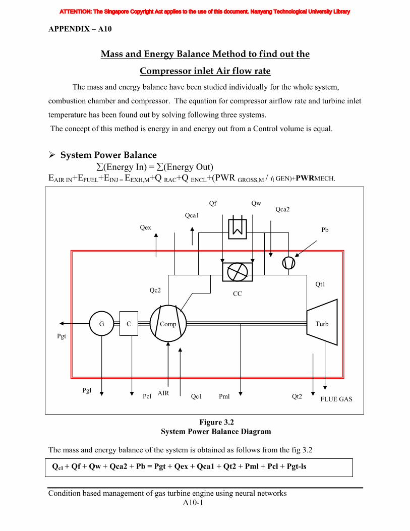
APPENDIX – A10
Mass and Energy Balance Method to find out the
Compressor inlet Air flow rate The mass and energy balance have been studied individually for the whole system,
combustion chamber and compressor. The equation for compressor airflow rate and turbine inlet
temperature has been found out by solving following three systems.
The concept of this method is energy in and energy out from a Control volume is equal.
System Power Balance ∑(Energy In) = ∑(Energy Out)
EAIR IN+EFUEL+EINJ = EEXH,M+Q RAC+Q ENCL+(PWR GROSS,M / ή GEN)+PWRMECH.
Pb
Qc2 Qt1
FLUE GASAIR
Qf Qca2
Qw
Qca1
Qex
Qt2 Qc1 Pml Pcl
Pgt
Pgl
CC
C Turb Comp G
Figure 3.2 System Power Balance Diagram The mass and energy balance of the system is obtained as follows from the fig 3.2
ATTENTION: The Singapore Copyright Act applies to the use of this document. Nanyang Technological University Library
Qc1 + Qf + Qw + Qca2 + Pb = Pgt + Qex + Qca1 + Qt2 + Pml + Pcl + Pgt-ls
Condition based management of gas turbine engine using neural networks A10-1
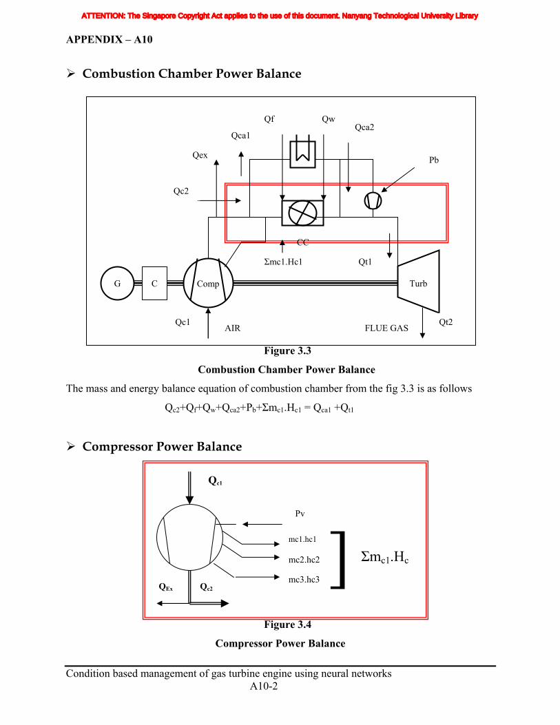
APPENDIX – A10
Combustion Chamber Power Balance
Figure 3.3
Qt2 Qc1
Qex
FLUE GAS AIR
Qt1 Σmc1.Hc1
Qc2
Pb
Qf Qca2
Qw
Qca1
CC
C Turb Comp G
Combustion Chamber Power Balance
The mass and energy balance equation of combustion chamber from the fig 3.3 is as follows
Qc2+Qf+Qw+Qca2+Pb+Σmc1.Hc1 = Qca1 +Qt1
Compressor Power Balance
Figure 3.4
QEx Qc2
Qc1
Σmc1.Hc]Pv
mc3.hc3
mc2.hc2
mc1.hc1
Compressor Power Balance Condition based management of gas turbine engine using neural networks A10-2
ATTENTION: The Singapore Copyright Act applies to the use of this document. Nanyang Technological University Library
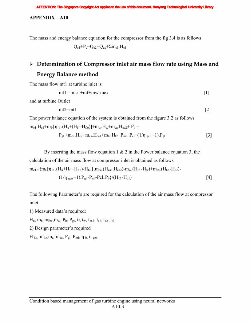
APPENDIX – A10
Condition based management of gas turbine engine using neural networks A10-3
The mass and energy balance equation for the compressor from the fig 3.4 is as follows
Qc1+Pc=Qc2+Qex+Σmc1.Hc1
Determination of Compressor inlet air mass flow rate using Mass and
Energy Balance method
The mass flow mt1 at turbine inlet is
mt1 = mc1+mf+mw-mex [1]
and at turbine Outlet
mt2=mt1 [2]
The power balance equation of the system is obtained from the figure 3.2 as follows
mc1.Hc1+mf.[η b .(Hu+(Hf –Hf,o)]+mw.Hw+mca.Hca2+ Pb =
Pgt +mex.Hc2+mca.Hca1+mt2.Ht2+Pml+Pcl+(1/η gen –1).Pgt [3]
By inserting the mass flow equation 1 & 2 in the Power balance equation 3, the
calculation of the air mass flow at compressor inlet is obtained as follows
mc1 ={mf.[η b .(Hu+Hf –Hf,o)-Ht2 ] -mca.(Hca1-Hca2)-mw.(Ht2 -Hw)+mex.(Ht2 -Hc2)-
(1/η gen –1).Pgt -Pml-Pcl+Pb}/(Ht2 -Hc1) [4]
The following Parameter’s are required for the calculation of the air mass flow at compressor
inlet
1) Measured data’s required:
Hu, mf, mEx ,mw, Pb, Pgt, tf, tw, tca2, tc1, tc2 , tt2
2) Design parameter’s required .
H f,o, mEn/mc, mca, Pgl, Pml, η b, η gen
ATTENTION: The Singapore Copyright Act applies to the use of this document. Nanyang Technological University Library
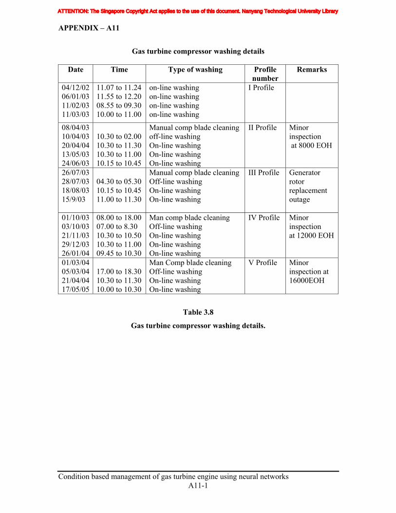
APPENDIX – A11
Gas turbine compressor washing details
Date Time Type of washing Profile number
Remarks
04/12/02 06/01/03 11/02/03 11/03/03
11.07 to 11.24 11.55 to 12.20 08.55 to 09.30 10.00 to 11.00
on-line washing on-line washing on-line washing on-line washing
I Profile
08/04/03 10/04/03 20/04/04 13/05/03 24/06/03
10.30 to 02.00 10.30 to 11.30 10.30 to 11.00 10.15 to 10.45
Manual comp blade cleaning off-line washing On-line washing On-line washing On-line washing
II Profile Minor inspection at 8000 EOH
26/07/03 28/07/03 18/08/03 15/9/03
04.30 to 05.30 10.15 to 10.45 11.00 to 11.30
Manual comp blade cleaning Off-line washing On-line washing On-line washing
III Profile Generator rotor replacement outage
01/10/03 03/10/03 21/11/03 29/12/03 26/01/04
08.00 to 18.00 07.00 to 8.30 10.30 to 10.50 10.30 to 11.00 09.45 to 10.30
Man comp blade cleaning Off-line washing On-line washing On-line washing On-line washing
IV Profile Minor inspection at 12000 EOH
01/03/04 05/03/04 21/04/04 17/05/05
17.00 to 18.30 10.30 to 11.30 10.00 to 10.30
Man Comp blade cleaning Off-line washing On-line washing On-line washing
V Profile Minor inspection at 16000EOH
Table 3.8
Gas turbine compressor washing details.
Condition based management of gas turbine engine using neural networks
A11-1
ATTENTION: The Singapore Copyright Act applies to the use of this document. Nanyang Technological University Library

Appendix B
ATTENTION: The Singapore Copyright Act applies to the use of this document. Nanyang Technological University Library
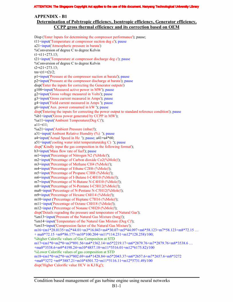
APPENDIX - B1 Determination of Polytropic efficiency, Isentropic efficiency, Generator efficiency,
CCPP gross thermal efficiency and its correction based on OEM Disp ('Enter Inputs for determining the compressor performance'); pause; t11=input('Temperature at compressor suction deg c'); pause a21=input('Atmospheric pressure in barata') %Conversion of degree C to degree Kelvin t1=t11+273.13; t21=input('Temperature at compressor discharge deg c'); pause %Conversion of degree C to degree Kelvin t2=t21+273.13; tm=(t1+t2)/2; p1=input('Pressure at the compressor suction at barata'); pause p2=input('Pressure at the compressor discharge at barata'); pause disp('Enter the inputs for correcting the Generator outputs') g100=input('Measured active power in MW'); pause g2=input('Gross voltage measured in Volts'); pause g3=input('Gross current measured in Amps'); pause g4=input('Field current measured in Amps '); pause g6=input('Aux. power consumed in kW '); pause disp('Entering the inputs for correcting the power output to standard reference condition'); pause %b1=input('Gross power generated by CCPP in MW'); %a11=input('Ambient Temperature(Deg C)'); a11=t11; %a21=input('Ambient Pressure (mbar)'); a31=input('Ambient Relative Humdity (%) '); pause a4=input('Actual Speed in Hz '); pause; a41=a4*60; a51=input('cooling water inlet temperature(deg C) '); pause disp(' Kindly input the gas composition in the following format'); b3=input('Mass flow rate of fuel'); pause m1=input('Percentage of Nitrogen N2 (%Mole)'); m2=input('Percentage of Carbon dioxide Co2(%Mole)'); m3=input('Percentage of Methane CH4 (%Mole)'); m4=input('Percentage of Ethane C2H6 (%Mole)'); m5=input('Percentage of Propane C3H8 (%Mole)'); m6=input('Percentage of I-Butane I-C4H10 (%Mole)'); m7=input('Percentage of N-Butane N-C4H10 (%Mole)'); m8=input('Percentage of N-Pentane I-C5H12(%Mole)'); ma8=input('Percentage of N-Pentane N-C5H12(%Mole)'); m9=input('Percentage of Hexane C6H14 (%Mole)'); m10=input ('Percentage of Heptane C7H16 (%Mole)'); m11=input('Percentage of Octane C8H18 (%Mole)'); m12=input ('Percentage of Nonane C9H20 (%Mole)'); disp('Details regrading the pressure and temperature of Natural Gas'); %m13=input('Pressure of the Natural Gas Mixture (barg)'); %m14=input('Temperature of the Natural Gas Mixture (Deg C)'); %m15=input('Compression factor of the Natural Gas Mixture'); m16=(m1*28.0135+m2*44.01+m3*16.043+m4*30.07+m5*44.097+m6*58.123+m7*58.123+m8*72.15 … + ma8*72.15 +m9*86.177+m10*100.204+m11*114.231+m12*128.258)/100; %higher Calorific values of Gas Compositon at STD m17=(m1*0+m2*0+m3*891.56+m4*1562.14+m5*2219.17+m6*2879.76+m7*2879.76+m8*3538.6 … +ma8*3538.6+m9*4198.24+m10*4857.18+m11*5516.01+m12*6175.82)/100 %Lower Calorific values of gas composition at STD m18=(m1*0+m2*0+m3*802.69+m4*1428.84+m5*2043.37+m6*2657.6+m7*2657.6+m8*3272 +ma8*3272 +m9*3887.21+m10*4501.72+m11*5116.11+m12*5731.49)/100 disp('Higher Calorific value HCV in KJ/Kg');
Condition based management of gas turbine engine using neural networks
B1-1
ATTENTION: The Singapore Copyright Act applies to the use of this document. Nanyang Technological University Library
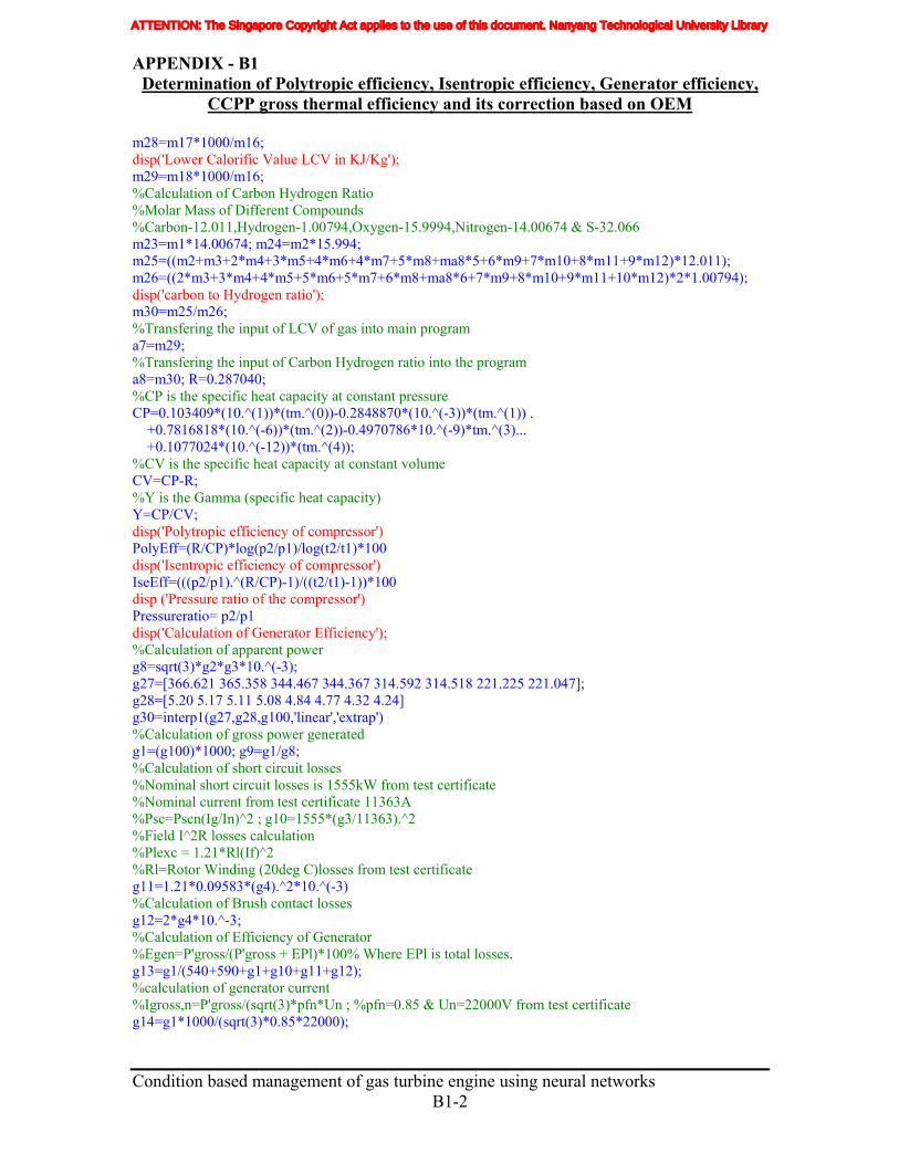
APPENDIX - B1 Determination of Polytropic efficiency, Isentropic efficiency, Generator efficiency,
CCPP gross thermal efficiency and its correction based on OEM m28=m17*1000/m16; disp('Lower Calorific Value LCV in KJ/Kg'); m29=m18*1000/m16; %Calculation of Carbon Hydrogen Ratio %Molar Mass of Different Compounds %Carbon-12.011,Hydrogen-1.00794,Oxygen-15.9994,Nitrogen-14.00674 & S-32.066 m23=m1*14.00674; m24=m2*15.994; m25=((m2+m3+2*m4+3*m5+4*m6+4*m7+5*m8+ma8*5+6*m9+7*m10+8*m11+9*m12)*12.011); m26=((2*m3+3*m4+4*m5+5*m6+5*m7+6*m8+ma8*6+7*m9+8*m10+9*m11+10*m12)*2*1.00794); disp('carbon to Hydrogen ratio'); m30=m25/m26; %Transfering the input of LCV of gas into main program a7=m29; %Transfering the input of Carbon Hydrogen ratio into the program a8=m30; R=0.287040; %CP is the specific heat capacity at constant pressure CP=0.103409*(10.^(1))*(tm.^(0))-0.2848870*(10.^(-3))*(tm.^(1)) . +0.7816818*(10.^(-6))*(tm.^(2))-0.4970786*10.^(-9)*tm.^(3)... +0.1077024*(10.^(-12))*(tm.^(4)); %CV is the specific heat capacity at constant volume CV=CP-R; %Y is the Gamma (specific heat capacity) Y=CP/CV; disp('Polytropic efficiency of compressor') PolyEff=(R/CP)*log(p2/p1)/log(t2/t1)*100 disp('Isentropic efficiency of compressor') IseEff=(((p2/p1).^(R/CP)-1)/((t2/t1)-1))*100 disp ('Pressure ratio of the compressor') Pressureratio= p2/p1 disp('Calculation of Generator Efficiency'); %Calculation of apparent power g8=sqrt(3)*g2*g3*10.^(-3); g27=[366.621 365.358 344.467 344.367 314.592 314.518 221.225 221.047]; g28=[5.20 5.17 5.11 5.08 4.84 4.77 4.32 4.24] g30=interp1(g27,g28,g100,'linear','extrap') %Calculation of gross power generated g1=(g100)*1000; g9=g1/g8; %Calculation of short circuit losses %Nominal short circuit losses is 1555kW from test certificate %Nominal current from test certificate 11363A %Psc=Pscn(Ig/In)^2 ; g10=1555*(g3/11363).^2 %Field I^2R losses calculation %Plexc = 1.21*Rl(If)^2 %Rl=Rotor Winding (20deg C)losses from test certificate g11=1.21*0.09583*(g4).^2*10.^(-3) %Calculation of Brush contact losses g12=2*g4*10.^-3; %Calculation of Efficiency of Generator %Egen=P'gross/(P'gross + EPl)*100% Where EPl is total losses. g13=g1/(540+590+g1+g10+g11+g12); %calculation of generator current %Igross,n=P'gross/(sqrt(3)*pfn*Un ; %pfn=0.85 & Un=22000V from test certificate g14=g1*1000/(sqrt(3)*0.85*22000);
Condition based management of gas turbine engine using neural networks
B1-2
ATTENTION: The Singapore Copyright Act applies to the use of this document. Nanyang Technological University Library
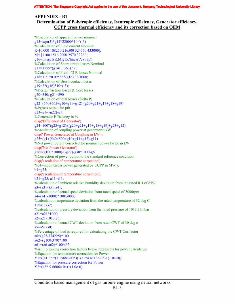
APPENDIX - B1 Determination of Polytropic efficiency, Isentropic efficiency, Generator efficiency,
CCPP gross thermal efficiency and its correction based on OEM %Caculation of apparent power nominal g15=sqrt(3)*g14*22000*10.^(-3) %Calculation of Field current Nominal R=[0.000 108250 216500 324750 433000]; M= [1100 1516 2000 2570 3226 ]; g16=interp1(R,M,g15,'linear','extrap') %Calculation of Short circuit losses Nominal g17=1555*(g14/11363).^2; %Calculation of Field I^2 R losses Nominal g18=1.21*0.09583*(g16).^2/1000; %Calculation of Brush contact losses g19=2*(g16)*10^(-3); %Design friction losses & Core losses g20=540; g21=590 %Calculation of total losses (Delta P) g22=(540+565+g10+g11+g12)-(g20+g21+g17+g18+g19) %Pgross output for pfn g23=g1-(-g22)-g11 %Generator Efficiency in % disp('Efficiency of Generator') g24=100*(g23+g12)/((g20+g21+g17+g18+g19)+g23+g12) %caculation of coupling power at generatorin kW disp(' Power Generated at Coupling in kW'); g25=(g1+(540+590+g10+g11+g12)-g11) %Net power output corrected for nominal power factor in kW disp('Net Power Generator') g26=(g100*1000)-(-g22)-g30*1000-g6 %Correction of power output to the standard reference condition disp('caculation of temperature correction'); %b1=input('Gross power generated by CCPP in MW'); b1=g25; disp('caculation of temperature correction'); b21=g25; a11=t11; %calculation of ambient relative humidity deviation from the rated RH of 85% a3=(a31-85); a41; %calculation of actual speed deviation from rated speed of 3000rpm a4=(a41-3000)*100/3000; %calculation temperature deviation from the rated temperature of 32 deg C a1=a11-32; %calculation of pressure deviation from the rated pressure of 1013.25mbar a21=a21*1000; a2=a21-1013.25; %calculation of actual CWT deviation from rated CWT of 30 deg c a5=a51-30; %Percentage of load is required for calculating the CWT Cor.factor a6=(g25/374225)*100 a62=(g100/370)*100 a61=(a6-a62)*100/a62; %All Following correction factors below represents for power calculation %Equation for temperature correction for Power Y1=((a1.^2 *(1.1568e-005))+(a1*4.4113e-03)+(1.0e-0)); %Equation for pressure correction for Power Y2=(a2*-9.6606e-04)+(1.0e-0);
Condition based management of gas turbine engine using neural networks
B1-3
ATTENTION: The Singapore Copyright Act applies to the use of this document. Nanyang Technological University Library
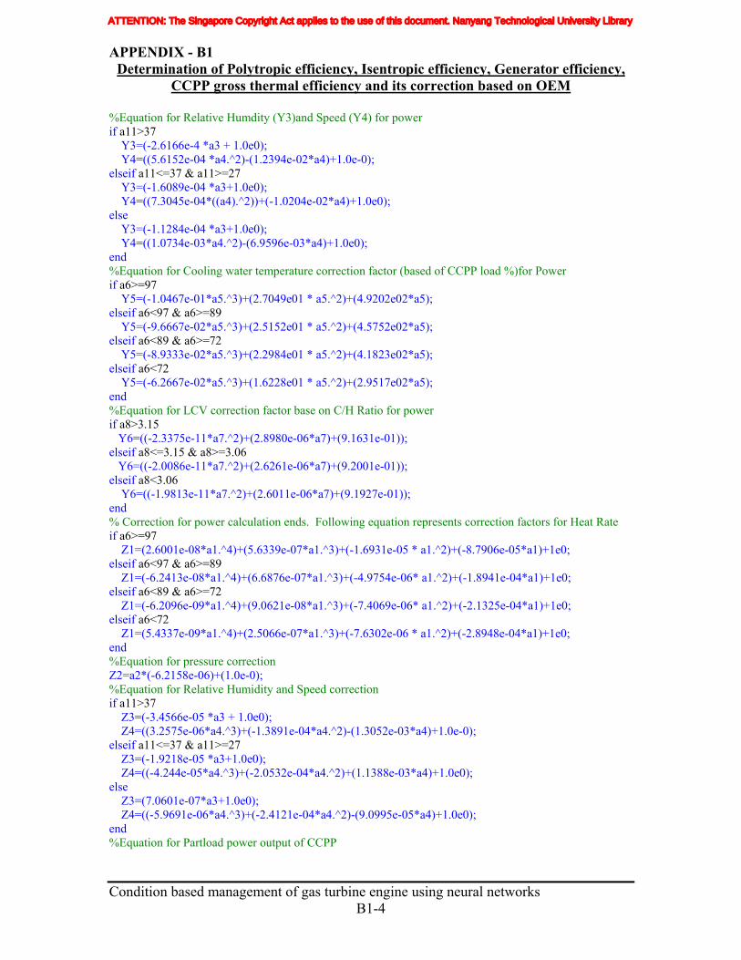
APPENDIX - B1 Determination of Polytropic efficiency, Isentropic efficiency, Generator efficiency,
CCPP gross thermal efficiency and its correction based on OEM %Equation for Relative Humdity (Y3)and Speed (Y4) for power if a11>37 Y3=(-2.6166e-4 *a3 + 1.0e0); Y4=((5.6152e-04 *a4.^2)-(1.2394e-02*a4)+1.0e-0); elseif a11<=37 & a11>=27 Y3=(-1.6089e-04 *a3+1.0e0); Y4=((7.3045e-04*((a4).^2))+(-1.0204e-02*a4)+1.0e0); else Y3=(-1.1284e-04 *a3+1.0e0); Y4=((1.0734e-03*a4.^2)-(6.9596e-03*a4)+1.0e0); end %Equation for Cooling water temperature correction factor (based of CCPP load %)for Power if a6>=97 Y5=(-1.0467e-01*a5.^3)+(2.7049e01 * a5.^2)+(4.9202e02*a5); elseif a6<97 & a6>=89 Y5=(-9.6667e-02*a5.^3)+(2.5152e01 * a5.^2)+(4.5752e02*a5); elseif a6<89 & a6>=72 Y5=(-8.9333e-02*a5.^3)+(2.2984e01 * a5.^2)+(4.1823e02*a5); elseif a6<72 Y5=(-6.2667e-02*a5.^3)+(1.6228e01 * a5.^2)+(2.9517e02*a5); end %Equation for LCV correction factor base on C/H Ratio for power if a8>3.15 Y6=((-2.3375e-11*a7.^2)+(2.8980e-06*a7)+(9.1631e-01)); elseif a8<=3.15 & a8>=3.06 Y6=((-2.0086e-11*a7.^2)+(2.6261e-06*a7)+(9.2001e-01)); elseif a8<3.06 Y6=((-1.9813e-11*a7.^2)+(2.6011e-06*a7)+(9.1927e-01)); end % Correction for power calculation ends. Following equation represents correction factors for Heat Rate if a6>=97 Z1=(2.6001e-08*a1.^4)+(5.6339e-07*a1.^3)+(-1.6931e-05 * a1.^2)+(-8.7906e-05*a1)+1e0; elseif a6<97 & a6>=89 Z1=(-6.2413e-08*a1.^4)+(6.6876e-07*a1.^3)+(-4.9754e-06* a1.^2)+(-1.8941e-04*a1)+1e0; elseif a6<89 & a6>=72 Z1=(-6.2096e-09*a1.^4)+(9.0621e-08*a1.^3)+(-7.4069e-06* a1.^2)+(-2.1325e-04*a1)+1e0; elseif a6<72 Z1=(5.4337e-09*a1.^4)+(2.5066e-07*a1.^3)+(-7.6302e-06 * a1.^2)+(-2.8948e-04*a1)+1e0; end %Equation for pressure correction Z2=a2*(-6.2158e-06)+(1.0e-0); %Equation for Relative Humidity and Speed correction if a11>37 Z3=(-3.4566e-05 *a3 + 1.0e0); Z4=((3.2575e-06*a4.^3)+(-1.3891e-04*a4.^2)-(1.3052e-03*a4)+1.0e-0); elseif a11<=37 & a11>=27 Z3=(-1.9218e-05 *a3+1.0e0); Z4=((-4.244e-05*a4.^3)+(-2.0532e-04*a4.^2)+(1.1388e-03*a4)+1.0e0); else Z3=(7.0601e-07*a3+1.0e0); Z4=((-5.9691e-06*a4.^3)+(-2.4121e-04*a4.^2)-(9.0995e-05*a4)+1.0e0); end %Equation for Partload power output of CCPP
Condition based management of gas turbine engine using neural networks
B1-4
ATTENTION: The Singapore Copyright Act applies to the use of this document. Nanyang Technological University Library
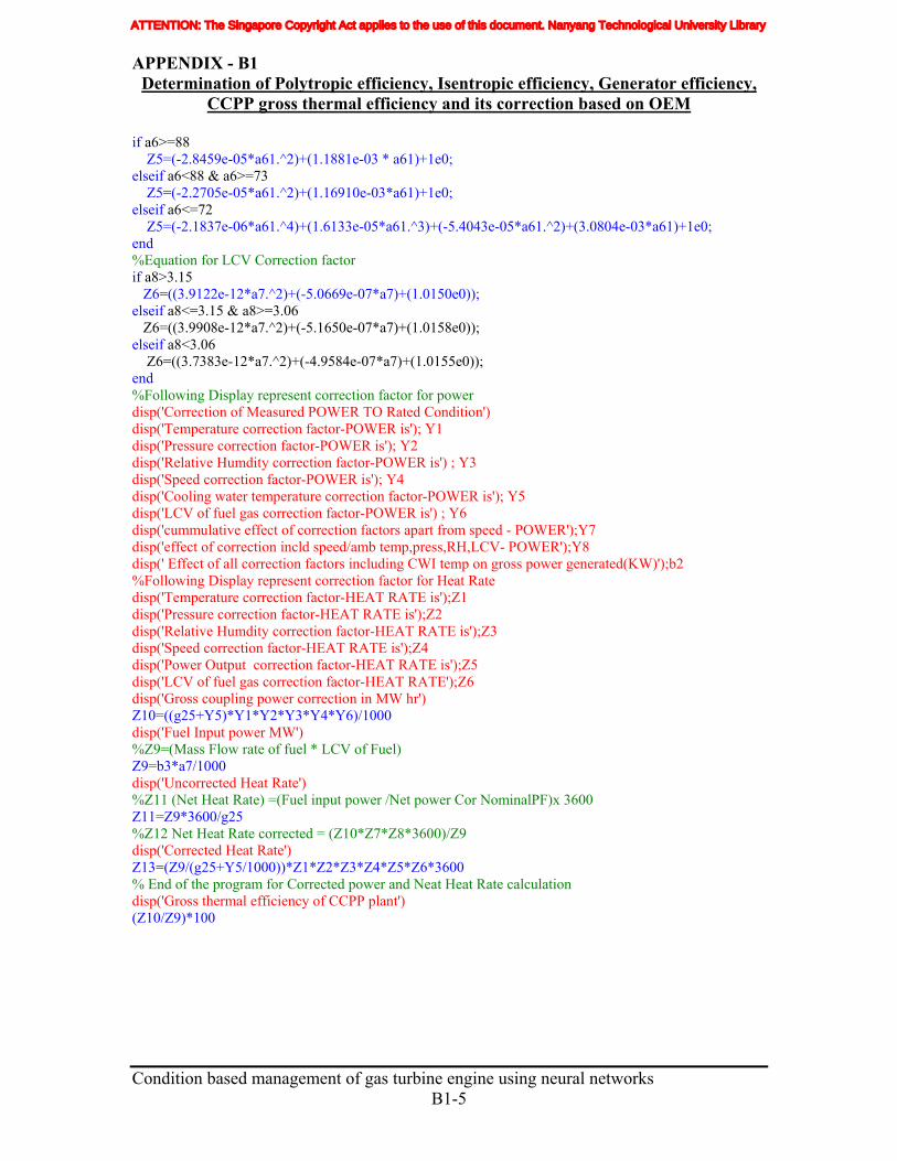
APPENDIX - B1 Determination of Polytropic efficiency, Isentropic efficiency, Generator efficiency,
CCPP gross thermal efficiency and its correction based on OEM
Condition based management of gas turbine engine using neural networks
B1-5
if a6>=88 Z5=(-2.8459e-05*a61.^2)+(1.1881e-03 * a61)+1e0; elseif a6<88 & a6>=73 Z5=(-2.2705e-05*a61.^2)+(1.16910e-03*a61)+1e0; elseif a6<=72 Z5=(-2.1837e-06*a61.^4)+(1.6133e-05*a61.^3)+(-5.4043e-05*a61.^2)+(3.0804e-03*a61)+1e0; end %Equation for LCV Correction factor if a8>3.15 Z6=((3.9122e-12*a7.^2)+(-5.0669e-07*a7)+(1.0150e0)); elseif a8<=3.15 & a8>=3.06 Z6=((3.9908e-12*a7.^2)+(-5.1650e-07*a7)+(1.0158e0)); elseif a8<3.06 Z6=((3.7383e-12*a7.^2)+(-4.9584e-07*a7)+(1.0155e0)); end %Following Display represent correction factor for power disp('Correction of Measured POWER TO Rated Condition') disp('Temperature correction factor-POWER is'); Y1 disp('Pressure correction factor-POWER is'); Y2 disp('Relative Humdity correction factor-POWER is') ; Y3 disp('Speed correction factor-POWER is'); Y4 disp('Cooling water temperature correction factor-POWER is'); Y5 disp('LCV of fuel gas correction factor-POWER is') ; Y6 disp('cummulative effect of correction factors apart from speed - POWER');Y7 disp('effect of correction incld speed/amb temp,press,RH,LCV- POWER');Y8 disp(' Effect of all correction factors including CWI temp on gross power generated(KW)');b2 %Following Display represent correction factor for Heat Rate disp('Temperature correction factor-HEAT RATE is');Z1 disp('Pressure correction factor-HEAT RATE is');Z2 disp('Relative Humdity correction factor-HEAT RATE is');Z3 disp('Speed correction factor-HEAT RATE is');Z4 disp('Power Output correction factor-HEAT RATE is');Z5 disp('LCV of fuel gas correction factor-HEAT RATE');Z6 disp('Gross coupling power correction in MW hr') Z10=((g25+Y5)*Y1*Y2*Y3*Y4*Y6)/1000 disp('Fuel Input power MW') %Z9=(Mass Flow rate of fuel * LCV of Fuel) Z9=b3*a7/1000 disp('Uncorrected Heat Rate') %Z11 (Net Heat Rate) =(Fuel input power /Net power Cor NominalPF)x 3600 Z11=Z9*3600/g25 %Z12 Net Heat Rate corrected = (Z10*Z7*Z8*3600)/Z9 disp('Corrected Heat Rate') Z13=(Z9/(g25+Y5/1000))*Z1*Z2*Z3*Z4*Z5*Z6*3600 % End of the program for Corrected power and Neat Heat Rate calculation disp('Gross thermal efficiency of CCPP plant') (Z10/Z9)*100
ATTENTION: The Singapore Copyright Act applies to the use of this document. Nanyang Technological University Library
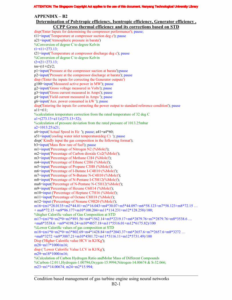
APPENDIX – B2 Determination of Polytropic efficiency, Isentropic efficiency, Generator efficiency ,
CCPP Gross thermal efficiency and its corrections based on STD disp('Enter Inputs for determining the compressor performance'); pause; t11=input('Temperature at compressor suction deg c'); pause a21=input('Atmospheric pressure in barata') %Conversion of degree C to degree Kelvin t1=t11+273.13; t21=input('Temperature at compressor discharge deg c'); pause %Conversion of degree C to degree Kelvin t2=t21+273.13; tm=(t1+t2)/2; p1=input('Pressure at the compressor suction at barata');pause p2=input('Pressure at the compressor discharge at barata'); pause disp ('Enter the inputs for correcting the Generator outputs') g100=input('Measured active power in MW'); pause g2=input('Gross voltage measured in Volts'); pause g3=input('Gross current measured in Amps'); pause g4=input('Field current measured in Amps '); pause g6=input('Aux. power consumed in kW '); pause disp('Entering the inputs for correcting the power output to standard reference condition'); pause a11=t11; %calculation temperature correction from the rated temperature of 32 deg C a1=(273.13+a11)/(273.13+32); %calculation of pressure deviation from the rated pressure of 1013.25mbar a2=1013.25/a21; a4=input('Actual Speed in Hz '); pause; a41=a4*60; a51=input('cooling water inlet temperature(deg C) '); pause disp(' Kindly input the gas composition in the following format'); b3=input('Mass flow rate of fuel'); pause m1=input('Percentage of Nitrogen N2 (%Mole)'); m2=input('Percentage of Carbon dioxide Co2(%Mole)'); m3=input('Percentage of Methane CH4 (%Mole)'); m4=input('Percentage of Ethane C2H6 (%Mole)'); m5=input('Percentage of Propane C3H8 (%Mole)'); m6=input('Percentage of I-Butane I-C4H10 (%Mole)'); m7=input('Percentage of N-Butane N-C4H10 (%Mole)'); m8=input('Percentage of N-Pentane I-C5H12(%Mole)'); ma8=input('Percentage of N-Pentane N-C5H12(%Mole)'); m9=input('Percentage of Hexane C6H14 (%Mole)'); m10=input ('Percentage of Heptane C7H16 (%Mole)'); m11=input('Percentage of Octane C8H18 (%Mole)'); m12=input ('Percentage of Nonane C9H20 (%Mole)'); m16=(m1*28.0135+m2*44.01+m3*16.043+m4*30.07+m5*44.097+m6*58.123+m7*58.123+m8*72.15 … + ma8*72.15 +m9*86.177+m10*100.204+m11*114.231+m12*128.258)/100; %higher Calorific values of Gas Composition at STD m17=(m1*0+m2*0+m3*891.56+m4*1562.14+m5*2219.17+m6*2879.76+m7*2879.76+m8*3538.6 … +ma8*3538.6 +m9*4198.24+m10*4857.18+m11*5516.01+m12*6175.82)/100 %Lower Calorific values of gas composition at STD m18=(m1*0+m2*0+m3*802.69+m4*1428.84+m5*2043.37+m6*2657.6+m7*2657.6+m8*3272 … +ma8*3272 +m9*3887.21+m10*4501.72+m11*5116.11+m12*5731.49)/100 Disp ('Higher Calorific value HCV in KJ/Kg'); m28=m17*1000/m16; disp ( 'Lower Calorific Value LCV in KJ/Kg'); m29=m18*1000/m16; %Calculation of Carbon Hydrogen Ratio andMolar Mass of Different Compounds %Carbon-12.011,Hydrogen-1.00794,Oxygen-15.9994,Nitrogen-14.00674 & S-32.066; m23=m1*14.00674; m24=m2*15.994;
________________________________________________________________________ Condition based management of gas turbine engine using neural networks
B2-1
ATTENTION: The Singapore Copyright Act applies to the use of this document. Nanyang Technological University Library
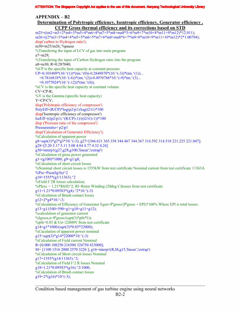
APPENDIX – B2 Determination of Polytropic efficiency, Isentropic efficiency, Generator efficiency ,
CCPP Gross thermal efficiency and its corrections based on STD m25=((m2+m3+2*m4+3*m5+4*m6+4*m7+5*m8+ma8*5+6*m9+7*m10+8*m11+9*m12)*12.011); m26=((2*m3+3*m4+4*m5+5*m6+5*m7+6*m8+ma8*6+7*m9+8*m10+9*m11+10*m12)*2*1.00794); disp('carbon to Hydrogen ratio'); m30=m25/m26; %pause %Transfering the input of LCV of gas into main program a7=m29; %Transfering the input of Carbon Hydrogen ratio into the program a8=m30; R=0.287040; %CP is the specific heat capacity at constant pressure CP=0.103409*(10.^(1))*(tm.^(0))-0.2848870*(10.^(-3))*(tm.^(1))... +0.7816818*(10.^(-6))*(tm.^(2))-0.4970786*10.^(-9)*tm.^(3)... +0.1077024*(10.^(-12))*(tm.^(4)); %CV is the specific heat capacity at constant volume CV=CP-R; %Y is the Gamma (specific heat capacity) Y=CP/CV; disp('Polytropic efficiency of compressor') PolyEff=(R/CP)*log(p2/p1)/log(t2/t1)*100 disp('Isentropic efficiency of compressor') IseEff=(((p2/p1).^(R/CP)-1)/((t2/t1)-1))*100 disp ('Pressure ratio of the compressor') Pressureratio= p2/p1 disp('Calculation of Generator Efficiency'); %Calculation of apparent power g8=sqrt(3)*g2*g3*10.^(-3); g27=[366.621 365.358 344.467 344.367 314.592 314.518 221.225 221.047]; g28=[5.20 5.17 5.11 5.08 4.84 4.77 4.32 4.24] g30=interp1(g27,g28,g100,'linear','extrap') %Calculation of gross power generated g1=(g100)*1000; g9=g1/g8; %Calculation of short circuit losses %Nominal short circuit losses is 1555kW from test certificate Nominal current from test certificate 11363A %Psc=Pscn(Ig/In)^2 g10=1555*(g3/11363).^2 %Field I^2R losses calculation; %Plexc = 1.21*Rl(If)^2; Rl=Rotor Winding (20deg C)losses from test certificate g11=1.21*0.09583*(g4).^2*10.^(-3) %Calculation of Brush contact losses g12=2*g4*10.^-3; %Calculation of Efficiency of Generator Egen=P'gross/(P'gross + EPl)*100% Where EPl is total losses. g13=g1/(540+590+g1+g10+g11+g12); %calculation of generator current %Igross,n=P'gross/(sqrt(3)*pfn*Un %pfn=0.85 & Un=22000V from test certificate g14=g1*1000/(sqrt(3)*0.85*22000); %Caculation of apparent power nominal g15=sqrt(3)*g14*22000*10.^(-3) %Calculation of Field current Nominal R=[0.000 108250 216500 324750 433000]; M= [1100 1516 2000 2570 3226 ]; g16=interp1(R,M,g15,'linear','extrap') %Calculation of Short circuit losses Nominal g17=1555*(g14/11363).^2; %Calculation of Field I^2 R losses Nominal g18=1.21*0.09583*(g16).^2/1000; %Calculation of Brush contact losses g19=2*(g16)*10^(-3);
________________________________________________________________________ Condition based management of gas turbine engine using neural networks
B2-2
ATTENTION: The Singapore Copyright Act applies to the use of this document. Nanyang Technological University Library
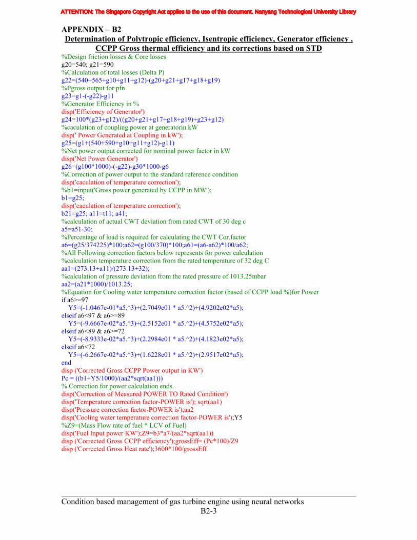
APPENDIX – B2 Determination of Polytropic efficiency, Isentropic efficiency, Generator efficiency ,
CCPP Gross thermal efficiency and its corrections based on STD
________________________________________________________________________ Condition based management of gas turbine engine using neural networks
B2-3
%Design friction losses & Core losses g20=540; g21=590 %Calculation of total losses (Delta P) g22=(540+565+g10+g11+g12)-(g20+g21+g17+g18+g19) %Pgross output for pfn g23=g1-(-g22)-g11 %Generator Efficiency in % disp('Efficiency of Generator') g24=100*(g23+g12)/((g20+g21+g17+g18+g19)+g23+g12) %caculation of coupling power at generatorin kW disp(' Power Generated at Coupling in kW'); g25=(g1+(540+590+g10+g11+g12)-g11) %Net power output corrected for nominal power factor in kW disp('Net Power Generator') g26=(g100*1000)-(-g22)-g30*1000-g6 %Correction of power output to the standard reference condition disp('caculation of temperature correction'); %b1=input('Gross power generated by CCPP in MW'); b1=g25; disp('caculation of temperature correction'); b21=g25; a11=t11; a41; %calculation of actual CWT deviation from rated CWT of 30 deg c a5=a51-30; %Percentage of load is required for calculating the CWT Cor.factor a6=(g25/374225)*100;a62=(g100/370)*100;a61=(a6-a62)*100/a62; %All Following correction factors below represents for power calculation %calculation temperature correction from the rated temperature of 32 deg C aa1=(273.13+a11)/(273.13+32); %calculation of pressure deviation from the rated pressure of 1013.25mbar aa2=(a21*1000)/1013.25; %Equation for Cooling water temperature correction factor (based of CCPP load %)for Power if a6>=97 Y5=(-1.0467e-01*a5.^3)+(2.7049e01 * a5.^2)+(4.9202e02*a5); elseif a6<97 & a6>=89 Y5=(-9.6667e-02*a5.^3)+(2.5152e01 * a5.^2)+(4.5752e02*a5); elseif a6<89 & a6>=72 Y5=(-8.9333e-02*a5.^3)+(2.2984e01 * a5.^2)+(4.1823e02*a5); elseif a6<72 Y5=(-6.2667e-02*a5.^3)+(1.6228e01 * a5.^2)+(2.9517e02*a5); end disp ('Corrected Gross CCPP Power output in KW') Pc = ((b1+Y5/1000)/(aa2*sqrt(aa1))) % Correction for power calculation ends. disp('Correction of Measured POWER TO Rated Condition') disp('Temperature correction factor-POWER is'); sqrt(aa1) disp('Pressure correction factor-POWER is');aa2 disp('Cooling water temperature correction factor-POWER is');Y5 %Z9=(Mass Flow rate of fuel * LCV of Fuel) disp('Fuel Input power KW');Z9=b3*a7/(aa2*sqrt(aa1)) disp ('Corrected Gross CCPP efficiency');grossEff= (Pc*100)/Z9 disp ('Corrected Gross Heat rate');3600*100/grossEff
ATTENTION: The Singapore Copyright Act applies to the use of this document. Nanyang Technological University Library
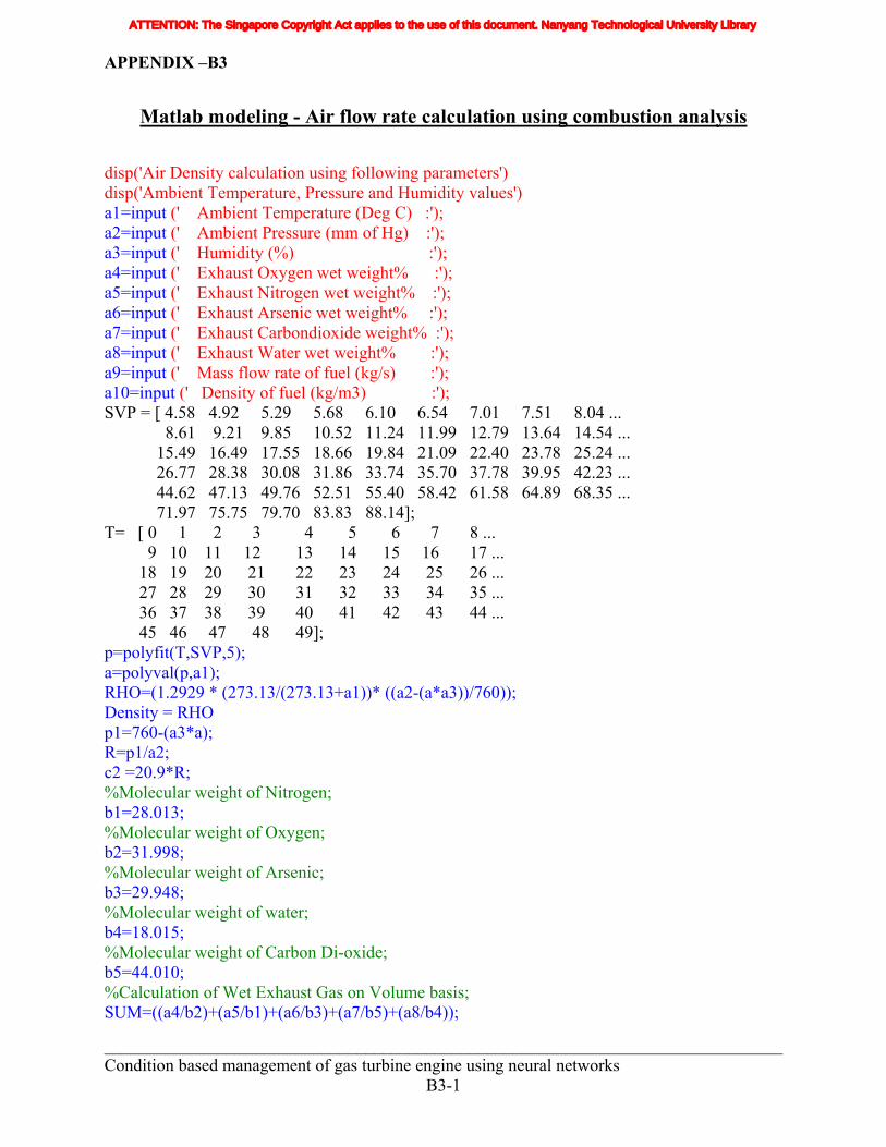
APPENDIX –B3
Matlab modeling - Air flow rate calculation using combustion analysis
disp('Air Density calculation using following parameters') disp('Ambient Temperature, Pressure and Humidity values') a1=input (' Ambient Temperature (Deg C) :'); a2=input (' Ambient Pressure (mm of Hg) :'); a3=input (' Humidity (%) :'); a4=input (' Exhaust Oxygen wet weight% :'); a5=input (' Exhaust Nitrogen wet weight% :'); a6=input (' Exhaust Arsenic wet weight% :'); a7=input (' Exhaust Carbondioxide weight% :'); a8=input (' Exhaust Water wet weight% :'); a9=input (' Mass flow rate of fuel (kg/s) :'); a10=input (' Density of fuel (kg/m3) :'); SVP = [ 4.58 4.92 5.29 5.68 6.10 6.54 7.01 7.51 8.04 ... 8.61 9.21 9.85 10.52 11.24 11.99 12.79 13.64 14.54 ... 15.49 16.49 17.55 18.66 19.84 21.09 22.40 23.78 25.24 ... 26.77 28.38 30.08 31.86 33.74 35.70 37.78 39.95 42.23 ... 44.62 47.13 49.76 52.51 55.40 58.42 61.58 64.89 68.35 ... 71.97 75.75 79.70 83.83 88.14]; T= [ 0 1 2 3 4 5 6 7 8 ... 9 10 11 12 13 14 15 16 17 ... 18 19 20 21 22 23 24 25 26 ... 27 28 29 30 31 32 33 34 35 ... 36 37 38 39 40 41 42 43 44 ... 45 46 47 48 49]; p=polyfit(T,SVP,5); a=polyval(p,a1); RHO=(1.2929 * (273.13/(273.13+a1))* ((a2-(a*a3))/760)); Density = RHO p1=760-(a3*a); R=p1/a2; c2 =20.9*R; %Molecular weight of Nitrogen; b1=28.013; %Molecular weight of Oxygen; b2=31.998; %Molecular weight of Arsenic; b3=29.948; %Molecular weight of water; b4=18.015; %Molecular weight of Carbon Di-oxide; b5=44.010; %Calculation of Wet Exhaust Gas on Volume basis; SUM=((a4/b2)+(a5/b1)+(a6/b3)+(a7/b5)+(a8/b4));
______________________________________________________________________________ Condition based management of gas turbine engine using neural networks
B3-1
ATTENTION: The Singapore Copyright Act applies to the use of this document. Nanyang Technological University Library
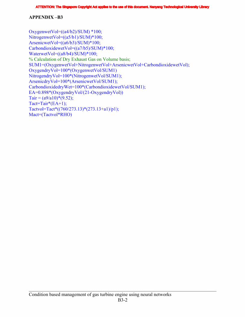
APPENDIX –B3
______________________________________________________________________________ Condition based management of gas turbine engine using neural networks
B3-2
OxygenwetVol=((a4/b2)/SUM) *100; NitrogenwetVol=((a5/b1)/SUM)*100; ArsenicwetVol=((a6/b3)/SUM)*100; CarbondioxidewetVol=((a7/b5)/SUM)*100; WaterwetVol=((a8/b4)/SUM)*100; % Calculation of Dry Exhaust Gas on Volume basis; SUM1=(OxygenwetVol+NitrogenwetVol+ArsenicwetVol+CarbondioxidewetVol); OxygendryVol=100*(OxygenwetVol/SUM1) NitrogendryVol=100*(NitrogenwetVol/SUM1); ArsenicdryVol=100*(ArsenicwetVol/SUM1); CarbondioxidedryWet=100*(CarbondioxidewetVol/SUM1); EA=0.898*(OxygendryVol/(21-OxygendryVol)) Tair = (a9/a10)*(9.52); Tact=Tair*(EA+1); Tactvol=Tact*((760/273.13)*(273.13+a1)/p1); Mact=(Tactvol*RHO)
ATTENTION: The Singapore Copyright Act applies to the use of this document. Nanyang Technological University Library
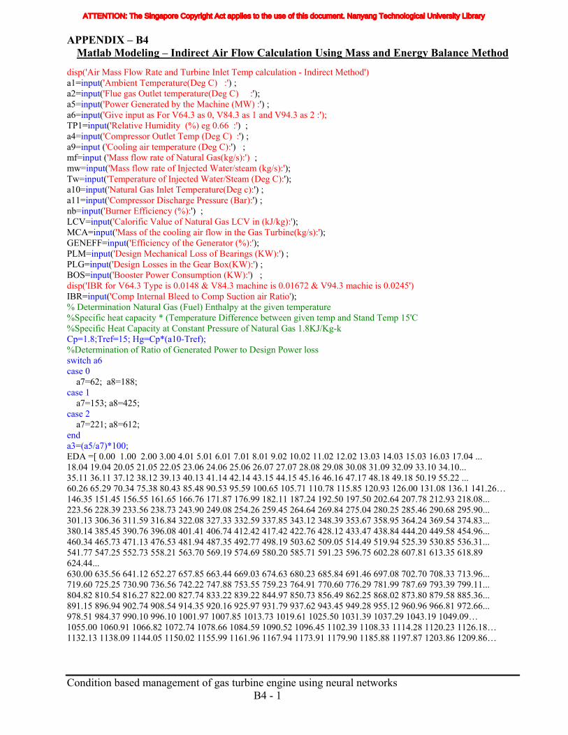
APPENDIX – B4 Matlab Modeling – Indirect Air Flow Calculation Using Mass and Energy Balance Method
disp('Air Mass Flow Rate and Turbine Inlet Temp calculation - Indirect Method') a1=input('Ambient Temperature(Deg C) :') ; a2=input('Flue gas Outlet temperature(Deg C) :'); a5=input('Power Generated by the Machine (MW) :') ; a6=input('Give input as For V64.3 as 0, V84.3 as 1 and V94.3 as 2 :'); TP1=input('Relative Humidity (%) eg 0.66 :') ; a4=input('Compressor Outlet Temp (Deg C) :') ; a9=input ('Cooling air temperature (Deg C):') ; mf=input ('Mass flow rate of Natural Gas(kg/s):') ; mw=input('Mass flow rate of Injected Water/steam (kg/s):'); Tw=input('Temperature of Injected Water/Steam (Deg C):'); a10=input('Natural Gas Inlet Temperature(Deg c):') ; a11=input('Compressor Discharge Pressure (Bar):') ; nb=input('Burner Efficiency (%):') ; LCV=input('Calorific Value of Natural Gas LCV in (kJ/kg):'); MCA=input('Mass of the cooling air flow in the Gas Turbine(kg/s):'); GENEFF=input('Efficiency of the Generator (%):'); PLM=input('Design Mechanical Loss of Bearings (KW):') ; PLG=input('Design Losses in the Gear Box(KW):') ; BOS=input('Booster Power Consumption (KW):') ; disp('IBR for V64.3 Type is 0.0148 & V84.3 machine is 0.01672 & V94.3 machie is 0.0245') IBR=input('Comp Internal Bleed to Comp Suction air Ratio'); % Determination Natural Gas (Fuel) Enthalpy at the given temperature %Specific heat capacity * (Temperature Difference between given temp and Stand Temp 15'C %Specific Heat Capacity at Constant Pressure of Natural Gas 1.8KJ/Kg-k Cp=1.8;Tref=15; Hg=Cp*(a10-Tref); %Determination of Ratio of Generated Power to Design Power loss switch a6 case 0 a7=62; a8=188; case 1 a7=153; a8=425; case 2 a7=221; a8=612; end a3=(a5/a7)*100; EDA =[ 0.00 1.00 2.00 3.00 4.01 5.01 6.01 7.01 8.01 9.02 10.02 11.02 12.02 13.03 14.03 15.03 16.03 17.04 ... 18.04 19.04 20.05 21.05 22.05 23.06 24.06 25.06 26.07 27.07 28.08 29.08 30.08 31.09 32.09 33.10 34.10... 35.11 36.11 37.12 38.12 39.13 40.13 41.14 42.14 43.15 44.15 45.16 46.16 47.17 48.18 49.18 50.19 55.22 ... 60.26 65.29 70.34 75.38 80.43 85.48 90.53 95.59 100.65 105.71 110.78 115.85 120.93 126.00 131.08 136.1 141.26… 146.35 151.45 156.55 161.65 166.76 171.87 176.99 182.11 187.24 192.50 197.50 202.64 207.78 212.93 218.08... 223.56 228.39 233.56 238.73 243.90 249.08 254.26 259.45 264.64 269.84 275.04 280.25 285.46 290.68 295.90... 301.13 306.36 311.59 316.84 322.08 327.33 332.59 337.85 343.12 348.39 353.67 358.95 364.24 369.54 374.83... 380.14 385.45 390.76 396.08 401.41 406.74 412.42 417.42 422.76 428.12 433.47 438.84 444.20 449.58 454.96... 460.34 465.73 471.13 476.53 481.94 487.35 492.77 498.19 503.62 509.05 514.49 519.94 525.39 530.85 536.31... 541.77 547.25 552.73 558.21 563.70 569.19 574.69 580.20 585.71 591.23 596.75 602.28 607.81 613.35 618.89 624.44... 630.00 635.56 641.12 652.27 657.85 663.44 669.03 674.63 680.23 685.84 691.46 697.08 702.70 708.33 713.96... 719.60 725.25 730.90 736.56 742.22 747.88 753.55 759.23 764.91 770.60 776.29 781.99 787.69 793.39 799.11... 804.82 810.54 816.27 822.00 827.74 833.22 839.22 844.97 850.73 856.49 862.25 868.02 873.80 879.58 885.36... 891.15 896.94 902.74 908.54 914.35 920.16 925.97 931.79 937.62 943.45 949.28 955.12 960.96 966.81 972.66... 978.51 984.37 990.10 996.10 1001.97 1007.85 1013.73 1019.61 1025.50 1031.39 1037.29 1043.19 1049.09… 1055.00 1060.91 1066.82 1072.74 1078.66 1084.59 1090.52 1096.45 1102.39 1108.33 1114.28 1120.23 1126.18… 1132.13 1138.09 1144.05 1150.02 1155.99 1161.96 1167.94 1173.91 1179.90 1185.88 1197.87 1203.86 1209.86…
Condition based management of gas turbine engine using neural networks B4 - 1
ATTENTION: The Singapore Copyright Act applies to the use of this document. Nanyang Technological University Library

APPENDIX – B4 Matlab Modeling – Indirect Air Flow Calculation Using Mass and Energy Balance Method
1215.86 1221.86 1227.87 1233.88 1239.89 1245.91 1251.93 1257.95 1263.98 1270.01 1276.04 1282.07 1288.11… 1294.15 1300.19 1306.23 1312.28 1318.33 1324.38]; T=[ 0 1 2 3 4 5 6 7 8 9 10 11 12 13 14 15 16 17 18 19 20 21 22 23 24 25 26 27 28 29 30 31 32 33… 34 35 36 37 38 39 40 41 42 43 44 45 46 47 48 49 50 55 60 65 70 75 80 85 90 95 100 105 110 115 120 125… 130 135 140 145 150 155 160 165 170 175 180 185 190 195 200 205 210 215 220 225 230 235 240 245 250 255… 260 265 270 275 280 285 290 295 300 305 310 315 320 325 330 335 340 345 350 355 360 365 370 375 380 385… 390 395 400 405 410 415 420 425 430 435 440 445 450 455 460 465 470 475 480 485 490 495 500 505 510 515… 520 525 530 535 540 545 550 560 565 570 575 580 585 590 595 600 605 610 615 620 625 630 635 640 645 650… 655 660 665 670 675 680 685 690 695 700 705 710 715 720 725 730 735 740 745 750 755 760 765 770 775 780 … 785 790 795 800 805 810 815 820 825 830 835 840 845 850 855 860 865 870 875 880 885 890 895 900 905 910… 915 920 925 930 935 940 945 950 955 960 965 970 975 980 990 995 1000 1005 1010 1015 1020 1025 1030… 1035 1040 1045 1050 1055 1060 1065 1070 1075 1080 1085 1090 1095 1100 1105 1110 1115 1120 1125 1130… 1135 1140 1145 1150 1155 1160 1165 1170 1175 1180 1185 1190 1195]; p=polyfit(T,EDA,7); B=polyval(p,a1) EWV = [0.00 1.86 3.72 5.58 7.44 9.30 11.16 13.02 14.88 16.74 18.60 20.47 22.33 24.19 26.05 27.92 29.78 31.64… 33.51 35.37 37.24 39.10 40.97 42.83 44.70 46.57 48.43 50.30 52.17 54.30 55.90 57.77 59.64 61.51 63.38 65.25… 67.12 68.99 70.866 72.73 74.60 76.47 78.34 80.21 82.09 83.96 85.83 87.71 89.58 91.45 93.33 102.71 112.09… 121.49 130.90 140.31 149.74 159.17 168.61 178.07 187.53 197.01 206.49 215.99 225.50 235.02 244.55 254.09… 263.64 273.20 282.78 292.37 301.96 311.58 321.20 330.84 340.49 350.15 359.82 369.51 379.21 388.92 398.65… 408.39 418.14 427.91 437.69 447.49 457.29 467.12 476.95 486.80 496.67 506.55 516.44 526.35 536.28 546.22… 556.17 566.14 576.12 586.12 596.14 606.17 616.21 626.27 636.35 646.44 656.55 666.67 676.81 686.97 697.14… 707.33 717.54 727.76 737.99 748.25 758.52 768.80 779.11 789.43 799.76 810.12 820.49 830.87 841.28 851.70… 862.14 872.59 883.06 893.55 904.06 914.58 925.13 935.69 946.26 956.85 967.47 978.09 988.74 999.40 1010.09… 1020.78 1031.50 1042.24 1052.99 1063.76 1074.55 1085.35 1096.17 1107.02 1117.87 1128.75 1139.65 1150.56… 1161.49 1172.44 1183.40 1194.39 1205.39 1216.41 1227.45 1238.51 1249.58 1260.68 1271.79 1282.91 1294.06… 1305.23 1316.41 1327.61 1338.83 1350.07 1361.32 1372.60 1383.89 1395.20 1406.52 1417.87 1429.23 1440.61… 1452.01 1463.43 1474.87 1486.32 1497.79 1509.28 1520.79 1532.31 1543.86 1555.42 1567.00 1578.59 1590.21... 1601.84 1613.84 1625.16 1636.85 1648.55 1660.27 1672.01 1683.77 1695.54 1707.33 1719.14 1730.97 1742.81… 1754.67 1766.55 1778.45 1790.36 1802.30 1814.24 1826.21 1838.19 1850.19 1862.21 1874.25 1886.30 1898.37… 1910.45 1922.56 1934.68 1946.81 1958.97 1971.14 1983.33 1995.53 2007.75 2019.99 2032.24 2044.51 2056.80… 2069.11 2081.43 2093.76 2106.12 2118.49 2130.87 2143.27 2155.69 2168.13 2180.58 2193.04 2205.52 2218.02… 2230.54 2243.07 2255.61 2268.17 2280.75 2293.34 2305.95 2318.58 2331.22 2343.87 2356.54 2369.23 2381.93… 2394.64 2407.38 2420.12 2432.88 2445.66 2458.08 2471.26 2484.08 2496.91 2509.76 2522.63 2535.51 2548.40… 2561.31 2574.31 2587.17 2600.12 2613.09 2626.07 2639.07 ]; T1=[ 0 1 2 3 4 5 6 7 8 9 10 11 12 13 14 15 16 17 18 19 20 21 22 23 24 25 26 27 28 29 30 31 32 33 34… 35 36 37 38 39 40 41 42 43 44 45 46 47 48 49 50 55 60 65 70 75 80 85 90 95 100 105 110 115 120 125 130… 135 140 145 150 155 160 165 170 175 180 185 190 195 200 205 210 215 220 225 230 235 240 245 250 255… 260 265 270 275 280 285 290 295 300 305 310 315 320 325 330 335 340 345 350 355 360 365 370 375 380… 385 390 395 400 405 410 415 420 425 430 435 440 445 450 455 460 465 470 475 480 485 490 495 500 505 510… 515 520 525 530 535 540 545 550 555 560 565 570 575 580 585 590 595 600 605 610 615 620 625 630 635 640… 645 650 655 660 665 670 675 680 685 690 695 700 705 710 715 720 725 730 735 740 745 750 755 760 765 770… 775 780 785 790 795 800 805 810 815 820 825 830 835 840 845 850 855 860 865 870 875 880 885 890 895 900… 905 910 915 920 925 930 935 940 945 950 955 960 965 970 975 980 990 995 1000 1005 1010 1015 1020 1025… 1030 1035 1040 1045 1050 1055 1060 1065 1070 1075 1080 1085 1090 1095 1100 1105 1110 1115 1120 1125… 1130 1135 1140 1145 1150 1155 1160 1165 1170 1175 1180 1185 1190 1195 1200 ] ; p1=polyfit(T1,EWV,7); B1=polyval(p1,a1) EMG = [ 520.95 527.07 533.20 539.34 545.48 551.63 557.79 563.95 570.12 576.31 582.49 588.69 594.89 601.10… 607.32 613.55 619.78 626.03 632.27 638.53 644.80 651.07 657.35 663.63 669.93 676.23 682.54 688.86 695.18… 701.51 707.85 714.20 720.55 726.92 733.28 739.66 746.05 752.44 758.84 765.24 771.65 778.08 784.50 790.94… 797.94 803.83 810.29 816.75 823.22 829.70 836.19 842.19 849.18 855.68 862.20 868.72 875.25 881.78 888.32… 894.87 901.43 907.99 914.56 921.14 927.72 934.31 940.91 947.51 954.12 960.74 967.36 973.99 980.63 987.27… 993.93 1000.58 1007.25 1013.92 1020.59 1027.28 1033.96 1040.66 1047.36 1054.07 1060.79 1067.51 1074.24… 1080.97 1087.71 1094.46 1101.21 1107.97 1114.73 1121.50 1128.28 1135.06 1141.85 1148.65 1155.45 1162.25…
Condition based management of gas turbine engine using neural networks B4 - 2
ATTENTION: The Singapore Copyright Act applies to the use of this document. Nanyang Technological University Library
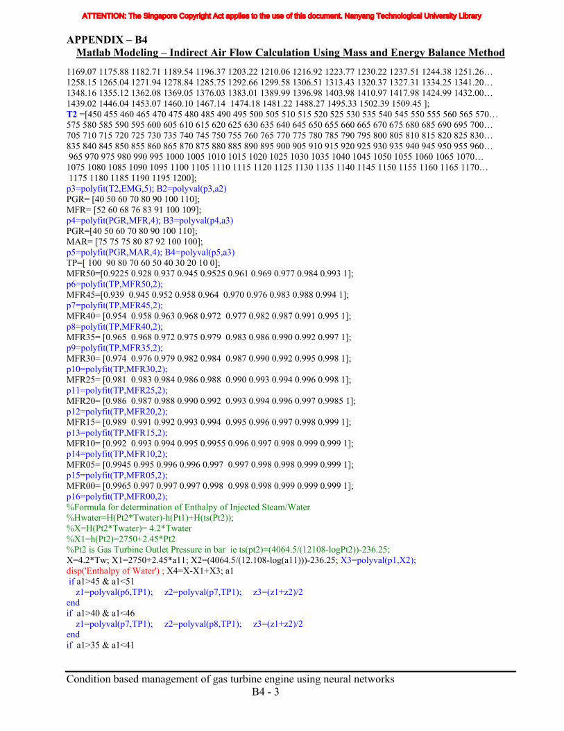
APPENDIX – B4 Matlab Modeling – Indirect Air Flow Calculation Using Mass and Energy Balance Method
1169.07 1175.88 1182.71 1189.54 1196.37 1203.22 1210.06 1216.92 1223.77 1230.22 1237.51 1244.38 1251.26… 1258.15 1265.04 1271.94 1278.84 1285.75 1292.66 1299.58 1306.51 1313.43 1320.37 1327.31 1334.25 1341.20… 1348.16 1355.12 1362.08 1369.05 1376.03 1383.01 1389.99 1396.98 1403.98 1410.97 1417.98 1424.99 1432.00… 1439.02 1446.04 1453.07 1460.10 1467.14 1474.18 1481.22 1488.27 1495.33 1502.39 1509.45 ]; T2 =[450 455 460 465 470 475 480 485 490 495 500 505 510 515 520 525 530 535 540 545 550 555 560 565 570… 575 580 585 590 595 600 605 610 615 620 625 630 635 640 645 650 655 660 665 670 675 680 685 690 695 700… 705 710 715 720 725 730 735 740 745 750 755 760 765 770 775 780 785 790 795 800 805 810 815 820 825 830… 835 840 845 850 855 860 865 870 875 880 885 890 895 900 905 910 915 920 925 930 935 940 945 950 955 960… 965 970 975 980 990 995 1000 1005 1010 1015 1020 1025 1030 1035 1040 1045 1050 1055 1060 1065 1070… 1075 1080 1085 1090 1095 1100 1105 1110 1115 1120 1125 1130 1135 1140 1145 1150 1155 1160 1165 1170… 1175 1180 1185 1190 1195 1200]; p3=polyfit(T2,EMG,5); B2=polyval(p3,a2) PGR= [40 50 60 70 80 90 100 110]; MFR= [52 60 68 76 83 91 100 109]; p4=polyfit(PGR,MFR,4); B3=polyval(p4,a3) PGR=[40 50 60 70 80 90 100 110]; MAR= [75 75 75 80 87 92 100 100]; p5=polyfit(PGR,MAR,4); B4=polyval(p5,a3) TP=[ 100 90 80 70 60 50 40 30 20 10 0]; MFR50=[0.9225 0.928 0.937 0.945 0.9525 0.961 0.969 0.977 0.984 0.993 1]; p6=polyfit(TP,MFR50,2); MFR45=[0.939 0.945 0.952 0.958 0.964 0.970 0.976 0.983 0.988 0.994 1]; p7=polyfit(TP,MFR45,2); MFR40= [0.954 0.958 0.963 0.968 0.972 0.977 0.982 0.987 0.991 0.995 1]; p8=polyfit(TP,MFR40,2); MFR35= [0.965 0.968 0.972 0.975 0.979 0.983 0.986 0.990 0.992 0.997 1]; p9=polyfit(TP,MFR35,2); MFR30= [0.974 0.976 0.979 0.982 0.984 0.987 0.990 0.992 0.995 0.998 1]; p10=polyfit(TP,MFR30,2); MFR25= [0.981 0.983 0.984 0.986 0.988 0.990 0.993 0.994 0.996 0.998 1]; p11=polyfit(TP,MFR25,2); MFR20= [0.986 0.987 0.988 0.990 0.992 0.993 0.994 0.996 0.997 0.9985 1]; p12=polyfit(TP,MFR20,2); MFR15= [0.989 0.991 0.992 0.993 0.994 0.995 0.996 0.997 0.998 0.999 1]; p13=polyfit(TP,MFR15,2); MFR10= [0.992 0.993 0.994 0.995 0.9955 0.996 0.997 0.998 0.999 0.999 1]; p14=polyfit(TP,MFR10,2); MFR05= [0.9945 0.995 0.996 0.996 0.997 0.997 0.998 0.998 0.999 0.999 1]; p15=polyfit(TP,MFR05,2); MFR00= [0.9965 0.997 0.997 0.997 0.998 0.998 0.998 0.999 0.999 0.999 1]; p16=polyfit(TP,MFR00,2); %Formula for determination of Enthalpy of Injected Steam/Water %Hwater=H(Pt2*Twater)-h(Pt1)+H(ts(Pt2)); %X=H(Pt2*Twater)= 4.2*Twater %X1=h(Pt2)=2750+2.45*Pt2 %Pt2 is Gas Turbine Outlet Pressure in bar ie ts(pt2)=(4064.5/(12108-logPt2))-236.25; X=4.2*Tw; X1=2750+2.45*a11; X2=(4064.5/(12.108-log(a11)))-236.25; X3=polyval(p1,X2); disp('Enthalpy of Water') ; X4=X-X1+X3; a1 if a1>45 & a1<51 z1=polyval(p6,TP1); z2=polyval(p7,TP1); z3=(z1+z2)/2 end if a1>40 & a1<46 z1=polyval(p7,TP1); z2=polyval(p8,TP1); z3=(z1+z2)/2 end if a1>35 & a1<41
Condition based management of gas turbine engine using neural networks B4 - 3
ATTENTION: The Singapore Copyright Act applies to the use of this document. Nanyang Technological University Library
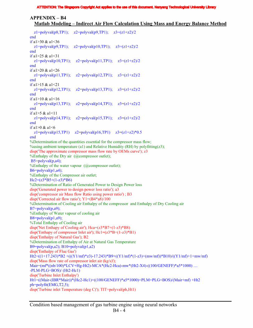
APPENDIX – B4 Matlab Modeling – Indirect Air Flow Calculation Using Mass and Energy Balance Method
Condition based management of gas turbine engine using neural networks B4 - 4
z1=polyval(p8,TP1); z2=polyval(p9,TP1); z3=(z1+z2)/2 end if a1>30 & a1<36 z1=polyval(p9,TP1); z2=polyval(p10,TP1); z3=(z1+z2)/2 end if a1>25 & a1<31 z1=polyval(p10,TP1); z2=polyval(p11,TP1); z3=(z1+z2)/2 end if a1>20 & a1<26 z1=polyval(p11,TP1); z2=polyval(p12,TP1); z3=(z1+z2)/2 end if a1>15 & a1<21 z1=polyval(p12,TP1); z2=polyval(p13,TP1); z3=(z1+z2)/2 end if a1>10 & a1<16 z1=polyval(p13,TP1); z2=polyval(p14,TP1); z3=(z1+z2)/2 end if a1>5 & a1<11 z1=polyval(p14,TP1); z2=polyval(p15,TP1); z3=(z1+z2)/2 end if a1>0 & a1<6 z1=polyval(p15,TP1) z2=polyval(p16,TP1) z3=(z1+z2)*0.5 end %Determination of the quantities essential for the compressor mass flow; %using ambient temperature (a1) and Relative Humidity (RH) by polyfitting(z3); disp('The approximate compressor mass flow rate by OEMs curve'); z3 %Enthalpy of the Dry air (@compressor outlet); B5=polyval(p,a4); %Enthalpy of the water vapour (@compressor outlet); B6=polyval(p1,a4); %Enthalpy of the Compressor air outlet; Hc2=(z3*B5+(1-z3)*B6) %Determination of Ratio of Generated Power to Design Power loss disp('Generated power to design power loss ratio'); a3 disp('compressor air Mass flow Ratio using power ratio') ; B3 disp('Corrected air flow ratio'); Y1=(B4*a8)/100 %Determination of Cooling air Enthalpy of the compressor and Enthalpy of Dry Cooling air B7=polyval(p,a9); %Enthalpy of Water vapour of cooling air B8=polyval(p1,a9); %Total Enthalpy of Cooling air disp('Net Enthapy of Cooling air'); Hca=(z3*B7+(1-z3)*B8) disp('Enthapy of compressor Inlet air'); Hc1=(z3*B+(1-z3)*B1) disp('Enthalpy of Natural Gas'); B2 %Determination of Enthalpy of Air at Natural Gas Temperature B9=polyval(p,a2); B10=polyval(p1,a2) disp('Enthalpy of Flue Gas') Ht2=((1+17.243)*B2 +(((Y1/mf)*z3)-17.243)*B9+((Y1/mf)*(1-z3)+(mw/mf))*B10)/((Y1/mf)+1+mw/mf) disp('Mass flow rate of compressor inlet air (kg/s)'); Mair=(mf*((nb/100)*LCV+Hg-Ht2)-MCA*(Hc2-Hca)-mw*(Ht2-X4)-((100/GENEFF)*a5*1000) … -PLM-PLG+BOS)/ (Ht2-Hc1) disp('Turbine Inlet Enthalpy') Ht1=((Mair-(IBR*Mair))*(Hc2-Hc1)+((100/GENEFF)*a5*1000)+PLM+PLG+BOS)/(Mair+mf) +Ht2 ph=polyfit(EMG,T2,5); disp('Turbine inlet Temperature (deg C)'); TIT=polyval(ph,Ht1)
ATTENTION: The Singapore Copyright Act applies to the use of this document. Nanyang Technological University Library
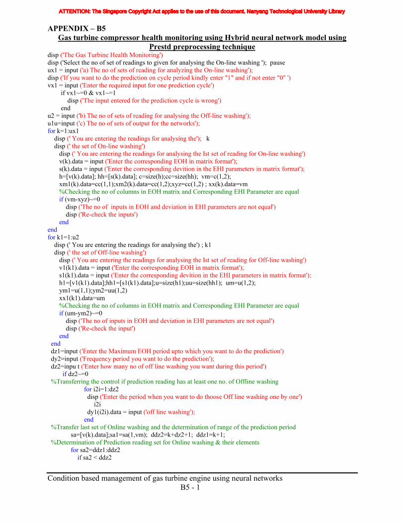
APPENDIX – B5 Gas turbine compressor health monitoring using Hybrid neural network model using
Prestd preprocessing technique disp ('The Gas Turbine Health Monitoring') disp ('Select the no of set of readings to given for analysing the On-line washing '); pause ux1 = input ('a) The no of sets of reading for analyzing the On-line washing'); disp ('If you want to do the prediction on cycle period kindly enter "1" and if not enter "0" ') vx1 = input ('Enter the required input for one prediction cycle') if vx1~=0 & vx1~=1 disp ('The input entered for the prediction cycle is wrong') end u2 = input ('b) The no of sets of reading for analysing the Off-line washing'); u1u=input ('c) The no of sets of output for the networks'); for k=1:ux1 disp (' You are entering the readings for analysing the'); k disp (' the set of On-line washing') disp (' You are entering the readings for analysing the Ist set of reading for On-line washing') v(k).data = input ('Enter the corresponding EOH in matrix format'); s(k).data = input ('Enter the corresponding devition in the EHI parameters in matrix format'); h=[v(k).data]; hh=[s(k).data]; c=size(h);cc=size(hh); vm=c(1,2); xm1(k).data=cc(1,1);xm2(k).data=cc(1,2);xyz=cc(1,2) ; xx(k).data=vm %Checking the no of columns in EOH matrix and Corresponding EHI Parameter are equal if (vm-xyz)~=0 disp ('The no of inputs in EOH and deviation in EHI parameters are not equal') disp ('Re-check the inputs') end end for k1=1:u2 disp (' You are entering the readings for analysing the') ; k1 disp (' the set of Off-line washing') disp (' You are entering the readings for analysing the Ist set of reading for Off-line washing') v1(k1).data = input ('Enter the corresponding EOH in matrix format'); s1(k1).data = input ('Enter the corresponding devition in the EHI parameters in matrix format'); h1=[v1(k1).data];hh1=[s1(k1).data];u=size(h1);uu=size(hh1); um=u(1,2); ym1=u(1,1);ym2=uu(1,2) xx1(k1).data=um %Checking the no of columns in EOH matrix and Corresponding EHI Parameter are equal if (um-ym2)~=0 disp ('The no of inputs in EOH and deviation in EHI parameters are not equal') disp ('Re-check the input') end end dz1=input ('Enter the Maximum EOH period upto which you want to do the prediction') dy2=input ('Frequency period you want to do the prediction'); dz2=inpu t ('Enter how many no of off line washing you want during this period') if dz2~=0 %Transferring the control if prediction reading has at least one no. of Offline washing for i2i=1:dz2 disp ('Enter the period when you want to do thoose Off line washing one by one') i2i dy1(i2i).data = input ('off line washing'); end %Transfer last set of Online washing and the determination of range of the prediction period sa=[v(k).data];sa1=sa(1,vm); ddz2=k+dz2+1; ddz1=k+1; %Determination of Prediction reading set for Online washing & their elements for sa2=ddz1:ddz2 if sa2 < ddz2 Condition based management of gas turbine engine using neural networks B5 - 1
ATTENTION: The Singapore Copyright Act applies to the use of this document. Nanyang Technological University Library
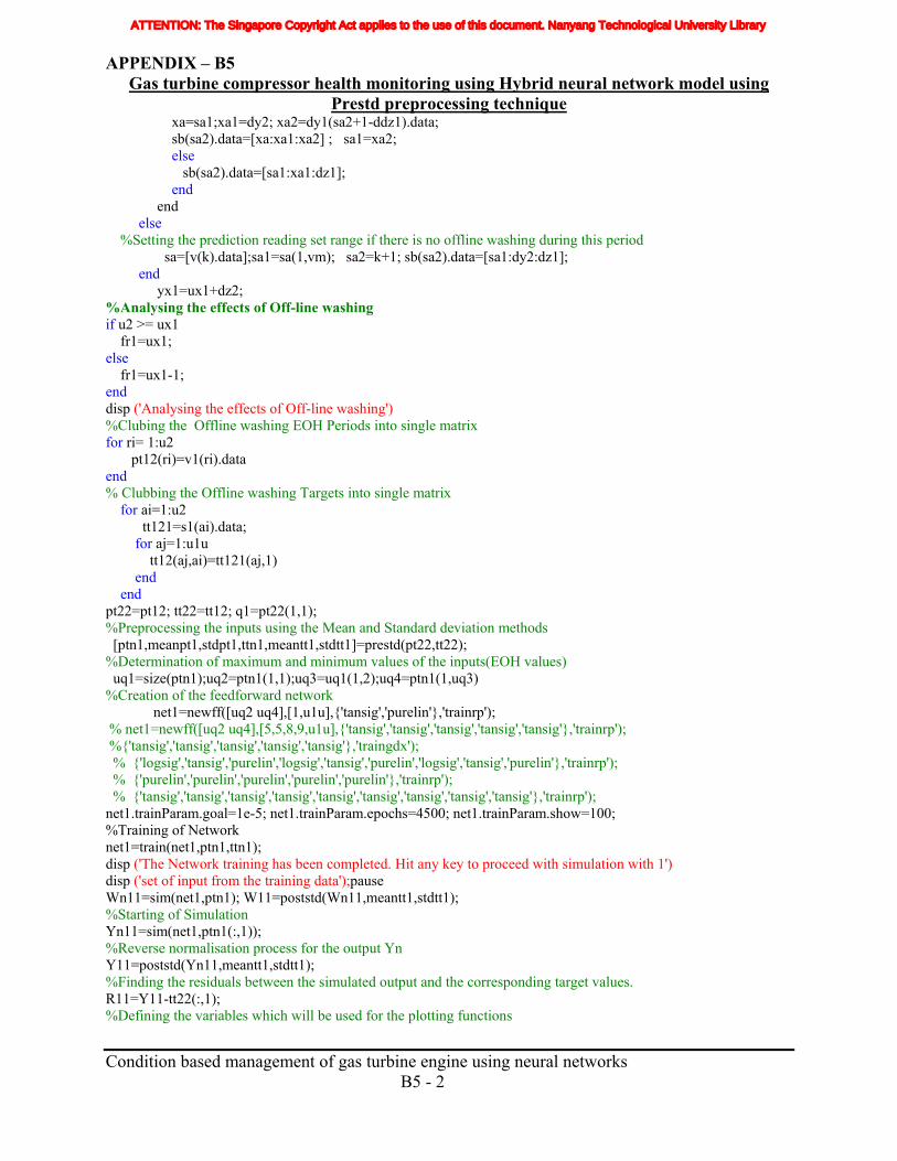
APPENDIX – B5 Gas turbine compressor health monitoring using Hybrid neural network model using
Prestd preprocessing technique xa=sa1;xa1=dy2; xa2=dy1(sa2+1-ddz1).data; sb(sa2).data=[xa:xa1:xa2] ; sa1=xa2; else sb(sa2).data=[sa1:xa1:dz1]; end end else %Setting the prediction reading set range if there is no offline washing during this period sa=[v(k).data];sa1=sa(1,vm); sa2=k+1; sb(sa2).data=[sa1:dy2:dz1]; end yx1=ux1+dz2; %Analysing the effects of Off-line washing if u2 >= ux1 fr1=ux1; else fr1=ux1-1; end disp ('Analysing the effects of Off-line washing') %Clubing the Offline washing EOH Periods into single matrix for ri= 1:u2 pt12(ri)=v1(ri).data end % Clubbing the Offline washing Targets into single matrix for ai=1:u2 tt121=s1(ai).data; for aj=1:u1u tt12(aj,ai)=tt121(aj,1) end end pt22=pt12; tt22=tt12; q1=pt22(1,1); %Preprocessing the inputs using the Mean and Standard deviation methods [ptn1,meanpt1,stdpt1,ttn1,meantt1,stdtt1]=prestd(pt22,tt22); %Determination of maximum and minimum values of the inputs(EOH values) uq1=size(ptn1);uq2=ptn1(1,1);uq3=uq1(1,2);uq4=ptn1(1,uq3) %Creation of the feedforward network net1=newff([uq2 uq4],[1,u1u],{'tansig','purelin'},'trainrp'); % net1=newff([uq2 uq4],[5,5,8,9,u1u],{'tansig','tansig','tansig','tansig','tansig'},'trainrp'); %{'tansig','tansig','tansig','tansig','tansig'},'traingdx'); % {'logsig','tansig','purelin','logsig','tansig','purelin','logsig','tansig','purelin'},'trainrp'); % {'purelin','purelin','purelin','purelin','purelin'},'trainrp'); % {'tansig','tansig','tansig','tansig','tansig','tansig','tansig','tansig','tansig'},'trainrp'); net1.trainParam.goal=1e-5; net1.trainParam.epochs=4500; net1.trainParam.show=100; %Training of Network net1=train(net1,ptn1,ttn1); disp ('The Network training has been completed. Hit any key to proceed with simulation with 1') disp ('set of input from the training data');pause Wn11=sim(net1,ptn1); W11=poststd(Wn11,meantt1,stdtt1); %Starting of Simulation Yn11=sim(net1,ptn1(:,1)); %Reverse normalisation process for the output Yn Y11=poststd(Yn11,meantt1,stdtt1); %Finding the residuals between the simulated output and the corresponding target values. R11=Y11-tt22(:,1); %Defining the variables which will be used for the plotting functions Condition based management of gas turbine engine using neural networks B5 - 2
ATTENTION: The Singapore Copyright Act applies to the use of this document. Nanyang Technological University Library
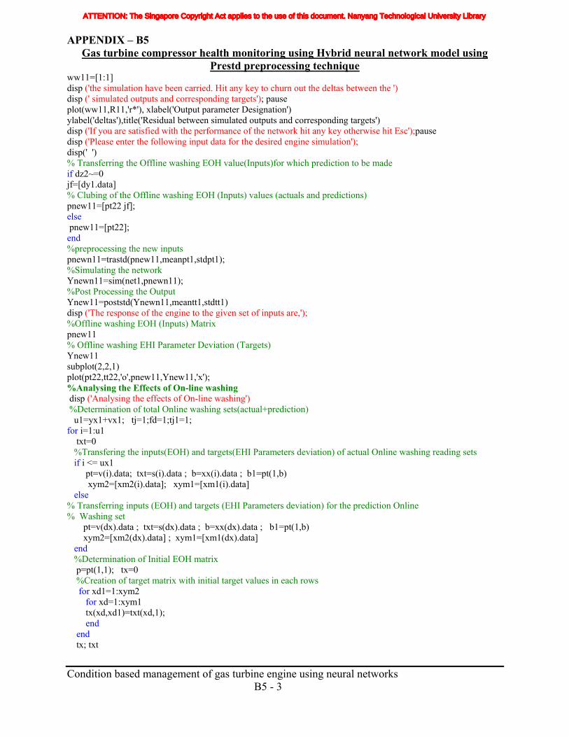
APPENDIX – B5 Gas turbine compressor health monitoring using Hybrid neural network model using
Prestd preprocessing technique ww11=[1:1] disp ('the simulation have been carried. Hit any key to churn out the deltas between the ') disp (' simulated outputs and corresponding targets'); pause plot(ww11,R11,'r*'), xlabel('Output parameter Designation') ylabel('deltas'),title('Residual between simulated outputs and corresponding targets') disp ('If you are satisfied with the performance of the network hit any key otherwise hit Esc');pause disp ('Please enter the following input data for the desired engine simulation'); disp(' ') % Transferring the Offline washing EOH value(Inputs)for which prediction to be made if dz2~=0 jf=[dy1.data] % Clubing of the Offline washing EOH (Inputs) values (actuals and predictions) pnew11=[pt22 jf]; else pnew11=[pt22]; end %preprocessing the new inputs pnewn11=trastd(pnew11,meanpt1,stdpt1); %Simulating the network Ynewn11=sim(net1,pnewn11); %Post Processing the Output Ynew11=poststd(Ynewn11,meantt1,stdtt1) disp ('The response of the engine to the given set of inputs are,'); %Offline washing EOH (Inputs) Matrix pnew11 % Offline washing EHI Parameter Deviation (Targets) Ynew11 subplot(2,2,1) plot(pt22,tt22,'o',pnew11,Ynew11,'x'); %Analysing the Effects of On-line washing disp ('Analysing the effects of On-line washing') %Determination of total Online washing sets(actual+prediction) u1=yx1+vx1; tj=1;fd=1;tj1=1; for i=1:u1 txt=0 %Transfering the inputs(EOH) and targets(EHI Parameters deviation) of actual Online washing reading sets if i <= ux1 pt=v(i).data; txt=s(i).data ; b=xx(i).data ; b1=pt(1,b) xym2=[xm2(i).data]; xym1=[xm1(i).data] else % Transferring inputs (EOH) and targets (EHI Parameters deviation) for the prediction Online % Washing set pt=v(dx).data ; txt=s(dx).data ; b=xx(dx).data ; b1=pt(1,b) xym2=[xm2(dx).data] ; xym1=[xm1(dx).data] end %Determination of Initial EOH matrix p=pt(1,1); tx=0 %Creation of target matrix with initial target values in each rows for xd1=1:xym2 for xd=1:xym1 tx(xd,xd1)=txt(xd,1); end end tx; txt Condition based management of gas turbine engine using neural networks B5 - 3
ATTENTION: The Singapore Copyright Act applies to the use of this document. Nanyang Technological University Library
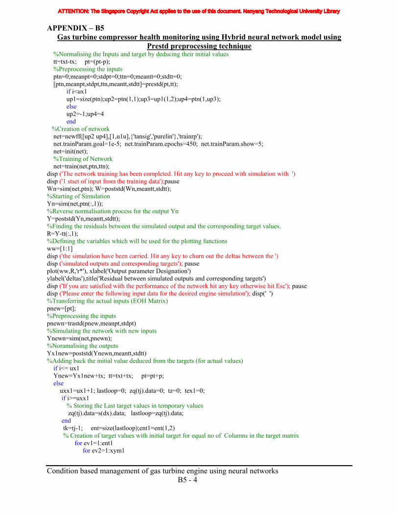
APPENDIX – B5 Gas turbine compressor health monitoring using Hybrid neural network model using
Prestd preprocessing technique %Normalising the Inputs and target by deducing their initial values tt=txt-tx; pt=(pt-p); %Preprocessing the inputs ptn=0;meanpt=0;stdpt=0;ttn=0;meantt=0;stdtt=0; [ptn,meanpt,stdpt,ttn,meantt,stdtt]=prestd(pt,tt); if i<ux1 up1=size(ptn);up2=ptn(1,1);up3=up1(1,2);up4=ptn(1,up3); else up2=-1;up4=4 end %Creation of network net=newff([up2 up4],[1,u1u],{'tansig','purelin'},'trainrp'); net.trainParam.goal=1e-5; net.trainParam.epochs=450; net.trainParam.show=5; net=init(net); %Training of Network net=train(net,ptn,ttn); disp ('The network training has been completed. Hit any key to proceed with simulation with ') disp ('1 stset of input from the training data');pause Wn=sim(net,ptn); W=poststd(Wn,meantt,stdtt); %Starting of Simulation Yn=sim(net,ptn(:,1)); %Reverse normalisation process for the output Yn Y=poststd(Yn,meantt,stdtt); %Finding the residuals between the simulated output and the corresponding target values. R=Y-tt(:,1); %Defining the variables which will be used for the plotting functions ww=[1:1] disp ('the simulation have been carried. Hit any key to churn out the deltas between the ') disp ('simulated outputs and corresponding targets'); pause plot(ww,R,'r*'), xlabel('Output parameter Designation') ylabel('deltas'),title('Residual between simulated outputs and corresponding targets') disp ('If you are satisfied with the performance of the network hit any key otherwise hit Esc'); pause disp ('Please enter the following input data for the desired engine simulation'); disp(' ') %Transferring the actual inputs (EOH Matrix) pnew=[pt]; %Preprocessing the inputs pnewn=trastd(pnew,meanpt,stdpt) %Simulating the network with new inputs Ynewn=sim(net,pnewn); %Noramalising the outputs Yx1new=poststd(Ynewn,meantt,stdtt) %Adding back the initial value deduced from the targets (for actual values) if i<= ux1 Ynew=Yx1new+tx; tt=txt+tx; pt=pt+p; else uxx1=ux1+1; lastloop=0; zq(tj).data=0; tz=0; tex1=0; if i>=uxx1 % Storing the Last target values in temporary values zq(tj).data=s(dx).data; lastloop=zq(tj).data; end tk=tj-1; ent=size(lastloop);ent1=ent(1,2) % Creation of target values with initial target for equal no of Columns in the target matrix for ev1=1:ent1 for ev2=1:xym1 Condition based management of gas turbine engine using neural networks B5 - 4
ATTENTION: The Singapore Copyright Act applies to the use of this document. Nanyang Technological University Library
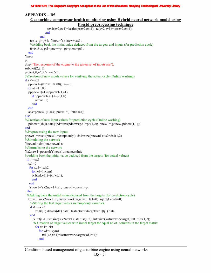
APPENDIX – B5 Gas turbine compressor health monitoring using Hybrid neural network model using
Prestd preprocessing technique tex1(ev2,ev1)=lastloop(ev2,ent1); tz(ev2,ev1)=txt(ev2,ent1); end end tex1; tj=tj+1; Ynew=Yx1new+tex1; %Adding back the initial value deduced from the targets and inputs (for prediction cycle) tt=txt+tx; pt1=pnew+p; pt=pnew+pt1; end Ynew pt disp ('The response of the engine to the given set of inputs are,'); subplot(2,2,1) plot(pt,tt,'o',pt,Ynew,'x'); %Creation of new inputs values for verifying the actual cycle (Online washing) if i <= ux1 ppnew1=(0:200:10000); aa=0; for a1=1:100 pppnew1(a1)=ppnew1(1,a1); if pppnew1(a1)<=pt(1,b) aa=aa+1; end end aaa=ppnew1(1,aa); pnew1=(0:200:aaa); else %Creation of new input values for prediction cycle (Online washing) pdnew=[sb(i).data]; pd=size(pdnew);pd1=pd(1,2); pnew1=(pdnew-pdnew(1,1)); end %Preprocessing the new inputs pnewn1=trastd(pnew1,meanpt,stdpt); ds1=size(pnewn1);ds2=ds1(1,2) %Simulating the network Ynewn1=sim(net,pnewn1); %Normalising the network Yx2new1=poststd(Ynewn1,meantt,stdtt); %Adding back the initial value deduced from the targets (for actual values) if i<=ux1 tx1=0 for xd1=1:ds2 for xd=1:xym1 tx1(xd,xd1)=txt(xd,1); end end Ynew1=Yx2new1+tx1; pnew1=pnew1+p; else %Adding back the initial value deduced from the targets (for prediction cycle) tx1=0; uxx2=ux1+1; lastnetworktarget=0; tx1=0; zq1(tj1).data=0; %Storing the last target values in temporary variables if i>=uxx2 zq1(tj1).data=s(dx).data; lastnetworktarget=zq1(tj1).data; end tk1=tj1-1; lst=size(Yx2new1);lst1=lst(1,2); lnt=size(lastnetworktarget);lnt1=lnt(1,2); % Creation of target values with initial target for equal no of columns in the target matrix for xd1=1:lst1 for xd=1:xym1 tx1(xd,xd1)=lastnetworktarget(xd,lnt1); end Condition based management of gas turbine engine using neural networks B5 - 5
ATTENTION: The Singapore Copyright Act applies to the use of this document. Nanyang Technological University Library
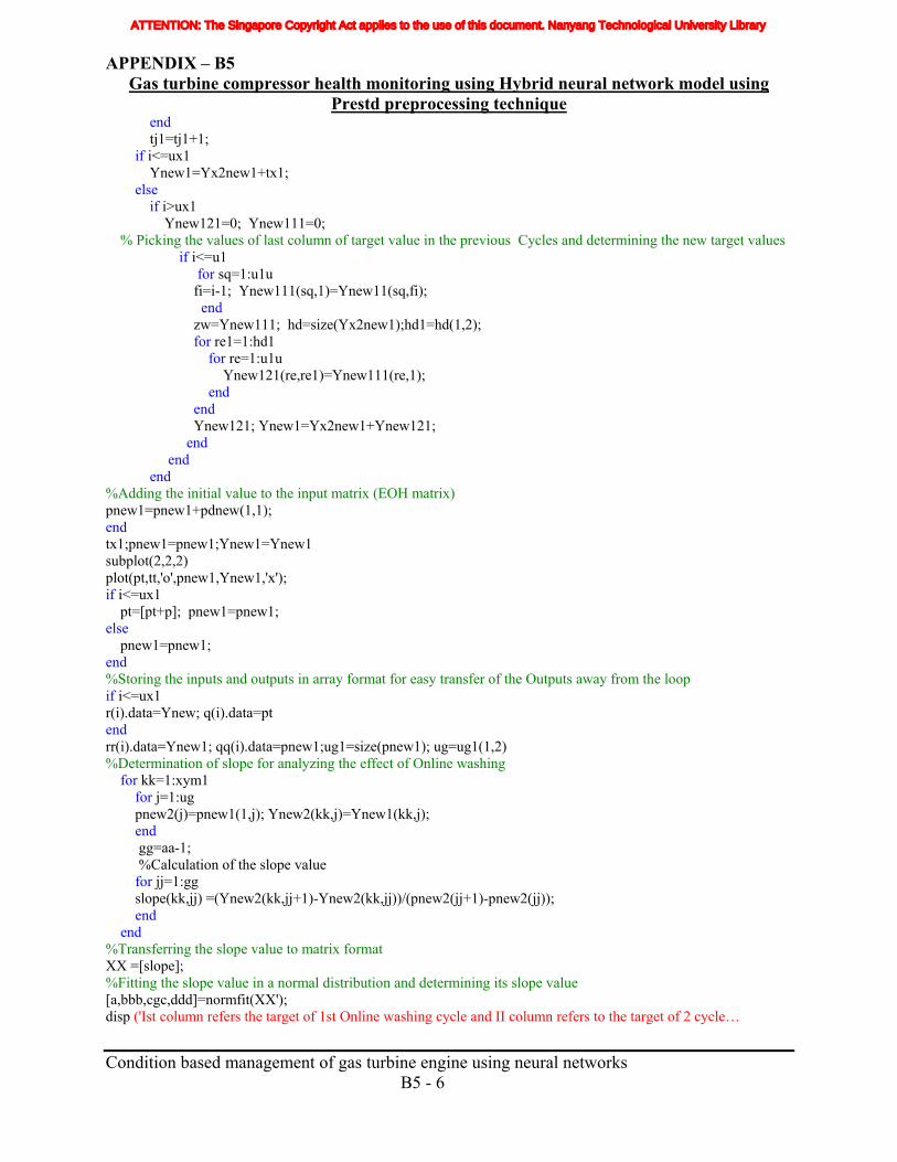
APPENDIX – B5 Gas turbine compressor health monitoring using Hybrid neural network model using
Prestd preprocessing technique end tj1=tj1+1; if i<=ux1 Ynew1=Yx2new1+tx1; else if i>ux1 Ynew121=0; Ynew111=0; % Picking the values of last column of target value in the previous Cycles and determining the new target values if i<=u1 for sq=1:u1u fi=i-1; Ynew111(sq,1)=Ynew11(sq,fi); end zw=Ynew111; hd=size(Yx2new1);hd1=hd(1,2); for re1=1:hd1 for re=1:u1u Ynew121(re,re1)=Ynew111(re,1); end end Ynew121; Ynew1=Yx2new1+Ynew121; end end end %Adding the initial value to the input matrix (EOH matrix) pnew1=pnew1+pdnew(1,1); end tx1;pnew1=pnew1;Ynew1=Ynew1 subplot(2,2,2) plot(pt,tt,'o',pnew1,Ynew1,'x'); if i<=ux1 pt=[pt+p]; pnew1=pnew1; else pnew1=pnew1; end %Storing the inputs and outputs in array format for easy transfer of the Outputs away from the loop if i<=ux1 r(i).data=Ynew; q(i).data=pt end rr(i).data=Ynew1; qq(i).data=pnew1;ug1=size(pnew1); ug=ug1(1,2) %Determination of slope for analyzing the effect of Online washing for kk=1:xym1 for j=1:ug pnew2(j)=pnew1(1,j); Ynew2(kk,j)=Ynew1(kk,j); end gg=aa-1; %Calculation of the slope value for jj=1:gg slope(kk,jj) =(Ynew2(kk,jj+1)-Ynew2(kk,jj))/(pnew2(jj+1)-pnew2(jj)); end end %Transferring the slope value to matrix format XX =[slope]; %Fitting the slope value in a normal distribution and determining its slope value [a,bbb,cgc,ddd]=normfit(XX'); disp ('Ist column refers the target of 1st Online washing cycle and II column refers to the target of 2 cycle… Condition based management of gas turbine engine using neural networks B5 - 6
ATTENTION: The Singapore Copyright Act applies to the use of this document. Nanyang Technological University Library
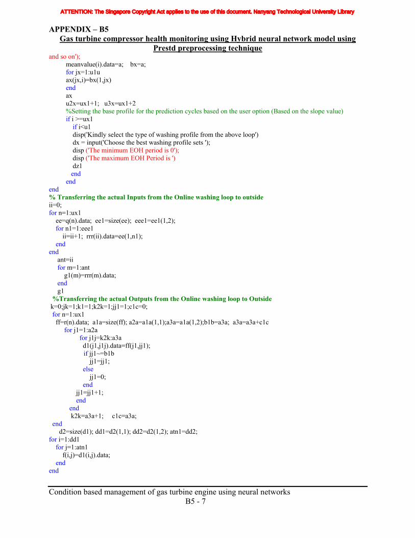
APPENDIX – B5 Gas turbine compressor health monitoring using Hybrid neural network model using
Prestd preprocessing technique and so on'); meanvalue(i).data=a; bx=a; for jx=1:u1u ax(jx,i)=bx(1,jx) end ax u2x=ux1+1; u3x=ux1+2 %Setting the base profile for the prediction cycles based on the user option (Based on the slope value) if i >=ux1 if i<u1 disp('Kindly select the type of washing profile from the above loop') dx = input('Choose the best washing profile sets '); disp ('The minimum EOH period is 0'); disp ('The maximum EOH Period is ') dz1 end end end % Transferring the actual Inputs from the Online washing loop to outside ii=0; for n=1:ux1 ee=q(n).data; ee1=size(ee); eee1=ee1(1,2); for n1=1:eee1 ii=ii+1; rrr(ii).data=ee(1,n1); end end ant=ii for m=1:ant g1(m)=rrr(m).data; end g1 %Transferring the actual Outputs from the Online washing loop to Outside k=0;jk=1;k1=1;k2k=1;jj1=1;c1c=0; for n=1:ux1 ff=r(n).data; a1a=size(ff); a2a=a1a(1,1);a3a=a1a(1,2);b1b=a3a; a3a=a3a+c1c for j1=1:a2a for j1j=k2k:a3a d1(j1,j1j).data=ff(j1,jj1);
if jj1~=b1b jj1=jj1; else jj1=0; end jj1=jj1+1; end end k2k=a3a+1; c1c=a3a; end d2=size(d1); dd1=d2(1,1); dd2=d2(1,2); atn1=dd2; for i=1:dd1 for j=1:atn1 f(i,j)=d1(i,j).data; end end Condition based management of gas turbine engine using neural networks B5 - 7
ATTENTION: The Singapore Copyright Act applies to the use of this document. Nanyang Technological University Library
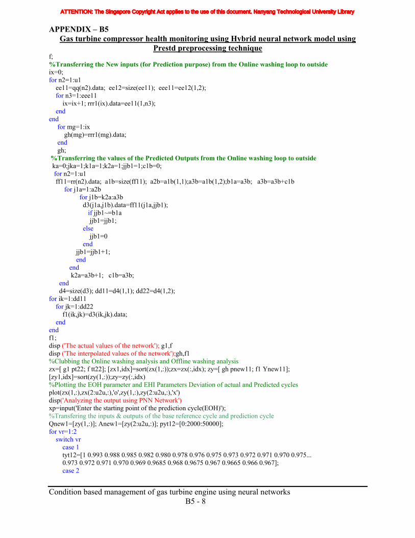
APPENDIX – B5 Gas turbine compressor health monitoring using Hybrid neural network model using
Prestd preprocessing technique f; %Transferring the New inputs (for Prediction purpose) from the Online washing loop to outside ix=0; for n2=1:u1 ee11=qq(n2).data; ee12=size(ee11); eee11=ee12(1,2); for n3=1:eee11 ix=ix+1; rrr1(ix).data=ee11(1,n3); end end for mg=1:ix gh(mg)=rrr1(mg).data; end gh; %Transferring the values of the Predicted Outputs from the Online washing loop to outside ka=0;jka=1;k1a=1;k2a=1;jjb1=1;c1b=0; for n2=1:u1 ff11=rr(n2).data; a1b=size(ff11); a2b=a1b(1,1);a3b=a1b(1,2);b1a=a3b; a3b=a3b+c1b for j1a=1:a2b for j1b=k2a:a3b d3(j1a,j1b).data=ff11(j1a,jjb1); if jjb1~=b1a jjb1=jjb1; else jjb1=0 end jjb1=jjb1+1; end end k2a=a3b+1; c1b=a3b; end d4=size(d3); dd11=d4(1,1); dd22=d4(1,2); for ik=1:dd11 for jk=1:dd22 f1(ik,jk)=d3(ik,jk).data; end end f1; disp ('The actual values of the network'); g1,f disp ('The interpolated values of the network');gh,f1 %Clubbing the Online washing analysis and Offline washing analysis zx=[ g1 pt22; f tt22]; [zx1,idx]=sort(zx(1,:));zx=zx(:,idx); zy=[ gh pnew11; f1 Ynew11]; [zy1,idx]=sort(zy(1,:));zy=zy(:,idx) %Plotting the EOH parameter and EHI Parameters Deviation of actual and Predicted cycles plot(zx(1,:),zx(2:u2u,:),'o',zy(1,:),zy(2:u2u,:),'x') disp('Analyzing the output using PNN Network') xp=input('Enter the starting point of the prediction cycle(EOH)'); %Transfering the inputs & outputs of the base reference cycle and prediction cycle Qnew1=[zy(1,:)]; Anew1=[zy(2:u2u,:)]; pyt12=[0:2000:50000]; for vr=1:2 switch vr case 1 tyt12=[1 0.993 0.988 0.985 0.982 0.980 0.978 0.976 0.975 0.973 0.972 0.971 0.970 0.975... 0.973 0.972 0.971 0.970 0.969 0.9685 0.968 0.9675 0.967 0.9665 0.966 0.967]; case 2 Condition based management of gas turbine engine using neural networks B5 - 8
ATTENTION: The Singapore Copyright Act applies to the use of this document. Nanyang Technological University Library
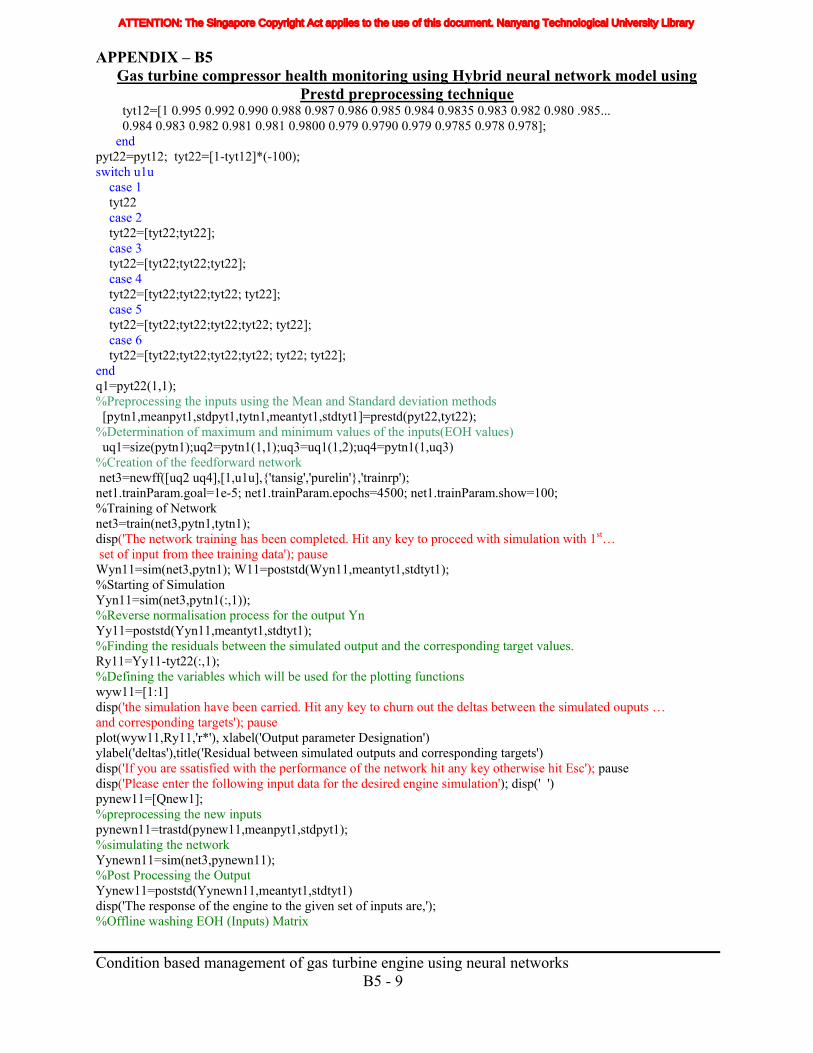
APPENDIX – B5 Gas turbine compressor health monitoring using Hybrid neural network model using
Prestd preprocessing technique tyt12=[1 0.995 0.992 0.990 0.988 0.987 0.986 0.985 0.984 0.9835 0.983 0.982 0.980 .985... 0.984 0.983 0.982 0.981 0.981 0.9800 0.979 0.9790 0.979 0.9785 0.978 0.978]; end pyt22=pyt12; tyt22=[1-tyt12]*(-100); switch u1u case 1 tyt22 case 2 tyt22=[tyt22;tyt22]; case 3 tyt22=[tyt22;tyt22;tyt22]; case 4 tyt22=[tyt22;tyt22;tyt22; tyt22]; case 5 tyt22=[tyt22;tyt22;tyt22;tyt22; tyt22]; case 6 tyt22=[tyt22;tyt22;tyt22;tyt22; tyt22; tyt22]; end q1=pyt22(1,1); %Preprocessing the inputs using the Mean and Standard deviation methods [pytn1,meanpyt1,stdpyt1,tytn1,meantyt1,stdtyt1]=prestd(pyt22,tyt22); %Determination of maximum and minimum values of the inputs(EOH values) uq1=size(pytn1);uq2=pytn1(1,1);uq3=uq1(1,2);uq4=pytn1(1,uq3) %Creation of the feedforward network net3=newff([uq2 uq4],[1,u1u],{'tansig','purelin'},'trainrp'); net1.trainParam.goal=1e-5; net1.trainParam.epochs=4500; net1.trainParam.show=100; %Training of Network net3=train(net3,pytn1,tytn1); disp('The network training has been completed. Hit any key to proceed with simulation with 1st… set of input from thee training data'); pause Wyn11=sim(net3,pytn1); W11=poststd(Wyn11,meantyt1,stdtyt1); %Starting of Simulation Yyn11=sim(net3,pytn1(:,1)); %Reverse normalisation process for the output Yn Yy11=poststd(Yyn11,meantyt1,stdtyt1); %Finding the residuals between the simulated output and the corresponding target values. Ry11=Yy11-tyt22(:,1); %Defining the variables which will be used for the plotting functions wyw11=[1:1] disp('the simulation have been carried. Hit any key to churn out the deltas between the simulated ouputs … and corresponding targets'); pause plot(wyw11,Ry11,'r*'), xlabel('Output parameter Designation') ylabel('deltas'),title('Residual between simulated outputs and corresponding targets') disp('If you are ssatisfied with the performance of the network hit any key otherwise hit Esc'); pause disp('Please enter the following input data for the desired engine simulation'); disp(' ') pynew11=[Qnew1]; %preprocessing the new inputs pynewn11=trastd(pynew11,meanpyt1,stdpyt1); %simulating the network Yynewn11=sim(net3,pynewn11); %Post Processing the Output Yynew11=poststd(Yynewn11,meantyt1,stdtyt1) disp('The response of the engine to the given set of inputs are,'); %Offline washing EOH (Inputs) Matrix Condition based management of gas turbine engine using neural networks B5 - 9
ATTENTION: The Singapore Copyright Act applies to the use of this document. Nanyang Technological University Library
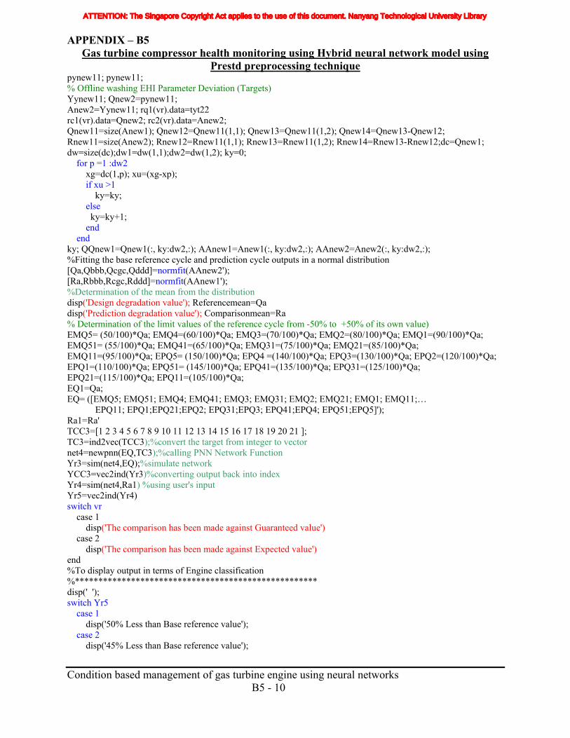
APPENDIX – B5 Gas turbine compressor health monitoring using Hybrid neural network model using
Prestd preprocessing technique pynew11; pynew11; % Offline washing EHI Parameter Deviation (Targets) Yynew11; Qnew2=pynew11; Anew2=Yynew11; rq1(vr).data=tyt22 rc1(vr).data=Qnew2; rc2(vr).data=Anew2; Qnew11=size(Anew1); Qnew12=Qnew11(1,1); Qnew13=Qnew11(1,2); Qnew14=Qnew13-Qnew12; Rnew11=size(Anew2); Rnew12=Rnew11(1,1); Rnew13=Rnew11(1,2); Rnew14=Rnew13-Rnew12;dc=Qnew1; dw=size(dc);dw1=dw(1,1);dw2=dw(1,2); ky=0; for p =1 :dw2 xg=dc(1,p); xu=(xg-xp); if xu >1 ky=ky; else ky=ky+1; end end ky; QQnew1=Qnew1(:, ky:dw2,:); AAnew1=Anew1(:, ky:dw2,:); AAnew2=Anew2(:, ky:dw2,:); %Fitting the base reference cycle and prediction cycle outputs in a normal distribution [Qa,Qbbb,Qcgc,Qddd]=normfit(AAnew2'); [Ra,Rbbb,Rcgc,Rddd]=normfit(AAnew1'); %Determination of the mean from the distribution disp('Design degradation value'); Referencemean=Qa disp('Prediction degradation value'); Comparisonmean=Ra % Determination of the limit values of the reference cycle from -50% to +50% of its own value) EMQ5= (50/100)*Qa; EMQ4=(60/100)*Qa; EMQ3=(70/100)*Qa; EMQ2=(80/100)*Qa; EMQ1=(90/100)*Qa; EMQ51= (55/100)*Qa; EMQ41=(65/100)*Qa; EMQ31=(75/100)*Qa; EMQ21=(85/100)*Qa; EMQ11=(95/100)*Qa; EPQ5= (150/100)*Qa; EPQ4 =(140/100)*Qa; EPQ3=(130/100)*Qa; EPQ2=(120/100)*Qa; EPQ1=(110/100)*Qa; EPQ51= (145/100)*Qa; EPQ41=(135/100)*Qa; EPQ31=(125/100)*Qa; EPQ21=(115/100)*Qa; EPQ11=(105/100)*Qa; EQ1=Qa; EQ= ([EMQ5; EMQ51; EMQ4; EMQ41; EMQ3; EMQ31; EMQ2; EMQ21; EMQ1; EMQ11;… EPQ11; EPQ1;EPQ21;EPQ2; EPQ31;EPQ3; EPQ41;EPQ4; EPQ51;EPQ5]'); Ra1=Ra' TCC3=[1 2 3 4 5 6 7 8 9 10 11 12 13 14 15 16 17 18 19 20 21 ]; TC3=ind2vec(TCC3);%convert the target from integer to vector net4=newpnn(EQ,TC3);%calling PNN Network Function Yr3=sim(net4,EQ);%simulate network YCC3=vec2ind(Yr3)%converting output back into index Yr4=sim(net4,Ra1) %using user's input Yr5=vec2ind(Yr4) switch vr case 1 disp('The comparison has been made against Guaranteed value') case 2 disp('The comparison has been made against Expected value') end %To display output in terms of Engine classification %**************************************************** disp(' '); switch Yr5 case 1 disp('50% Less than Base reference value'); case 2 disp('45% Less than Base reference value'); Condition based management of gas turbine engine using neural networks B5 - 10
ATTENTION: The Singapore Copyright Act applies to the use of this document. Nanyang Technological University Library
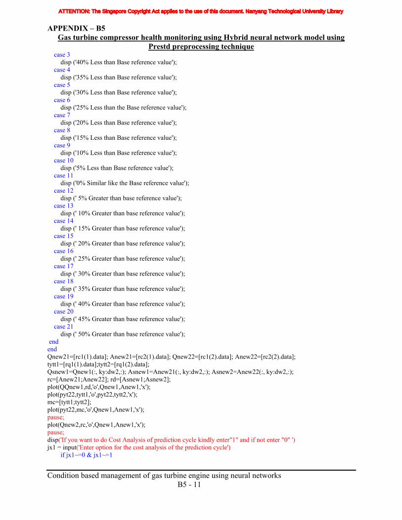
APPENDIX – B5 Gas turbine compressor health monitoring using Hybrid neural network model using
Prestd preprocessing technique case 3 disp ('40% Less than Base reference value'); case 4 disp ('35% Less than Base reference value'); case 5 disp ('30% Less than Base reference value'); case 6 disp ('25% Less than the Base reference value'); case 7 disp ('20% Less than Base reference value'); case 8 disp ('15% Less than Base reference value'); case 9 disp ('10% Less than Base reference value'); case 10 disp ('5% Less than Base reference value'); case 11 disp ('0% Similar like the Base reference value'); case 12 disp (' 5% Greater than base reference value'); case 13 disp (' 10% Greater than base reference value'); case 14 disp (' 15% Greater than base reference value'); case 15 disp (' 20% Greater than base reference value'); case 16 disp (' 25% Greater than base reference value'); case 17 disp (' 30% Greater than base reference value'); case 18 disp (' 35% Greater than base reference value'); case 19 disp (' 40% Greater than base reference value'); case 20 disp (' 45% Greater than base reference value'); case 21 disp (' 50% Greater than base reference value'); end end Qnew21=[rc1(1).data]; Anew21=[rc2(1).data]; Qnew22=[rc1(2).data]; Anew22=[rc2(2).data]; tytt1=[rq1(1).data];tytt2=[rq1(2).data]; Qsnew1=Qnew1(:, ky:dw2,:); Asnew1=Anew21(:, ky:dw2,:); Asnew2=Anew22(:, ky:dw2,:); rc=[Anew21;Anew22]; rd=[Asnew1;Asnew2]; plot(QQnew1,rd,'o',Qnew1,Anew1,'x'); plot(pyt22,tytt1,'o',pyt22,tytt2,'x'); mc=[tytt1;tytt2]; plot(pyt22,mc,'o',Qnew1,Anew1,'x'); pause; plot(Qnew2,rc,'o',Qnew1,Anew1,'x'); pause; disp('If you want to do Cost Analysis of prediction cycle kindly enter"1" and if not enter "0" ') jx1 = input('Enter option for the cost analysis of the prediction cycle') if jx1~=0 & jx1~=1 Condition based management of gas turbine engine using neural networks B5 - 11
ATTENTION: The Singapore Copyright Act applies to the use of this document. Nanyang Technological University Library

APPENDIX – B5 Gas turbine compressor health monitoring using Hybrid neural network model using
Prestd preprocessing technique
Condition based management of gas turbine engine using neural networks B5 - 12
disp('The input entered for the prediction cycle is wrong') end if jx1 > 0 mj=input('Kindly enter the average load per hour(MWhr'); uj1 = input('Enter the cost(S$/MWhr) of the production for the power generation'); uj2 = input('Enter the cost(S$/MWhr of Energy production)of the Fuel- Natural gas') uj3=input('Enter the cost(S$) of the Online washing=Chemical cost+ Manpower cost'); uj4=input('Enter the cost(S$)of the Offline washing + Manual Cleaning of IGV Blade -Chemical cost + Manpower cost'); disp('The Opportunity lost cost(S$) due to Offline washing + Manual Cleaning of IGV Blade'); uy1=input('The no of days the power generation has been lost because of IGV Blade cleaning and Offline washing'); disp( 'Two days of power generation were lost because of Manual Cleaning of IGV Blade+Offline washing'); uj5=(uj1-uj2)*24*uy1*mj disp('Net cost spend(S$) by doing Offline + IGV Blade cleaning'); uj6=uj5+uj4 disp('Net cost (S$)spent for doing Online washing'); uj3 disp('No of Online washing performed in the prediction period'); rf7=round(rf6) disp('No of Offline washing performed in the prediction period') ;dz2 disp('Total Cost(S$) spent for Online washing');hf1=rf7*uj3 disp('Total Cost(S$) spent for Offline washing'); hf2=dz2*(uj4+uj5) disp('Total Cost(S$) spent for both Online washing + Offline washing');hf=hf1+hf2 er1=Qnew1(:, ky:dw2,:); er2=Anew1(:, ky:dw2,:); er3=Anew22(:, ky:dw2,:); er4=-(er3-er2); plot(Qsnew1,rd,'o',Qnew1,Anew1,'x'); %Conversion of % Deviation to actual value er5=mj*dy2*er4/100; wr1=size(er5);wr2=wr1(1,2); qr1=[er1];qr2=[er2;er3;er4]; wr=0; for as=1:wr2 wr = wr+er5(1,as); end disp('Cummulative (MWhr) of energy wasted with reference to the reference washing… profile');wr disp('Cummulative amount(S$)of cost wasted(-) or cost gained(+) because of the energy lost');wq1=wr*uj1 disp('Net amount of money(S$) profitted(+) or Lost(-)due to the washing profile selected in the... prediction part'); wq2=wq1-hf disp(' The end of the program'); end
ATTENTION: The Singapore Copyright Act applies to the use of this document. Nanyang Technological University Library

Appendix C
ATTENTION: The Singapore Copyright Act applies to the use of this document. Nanyang Technological University Library
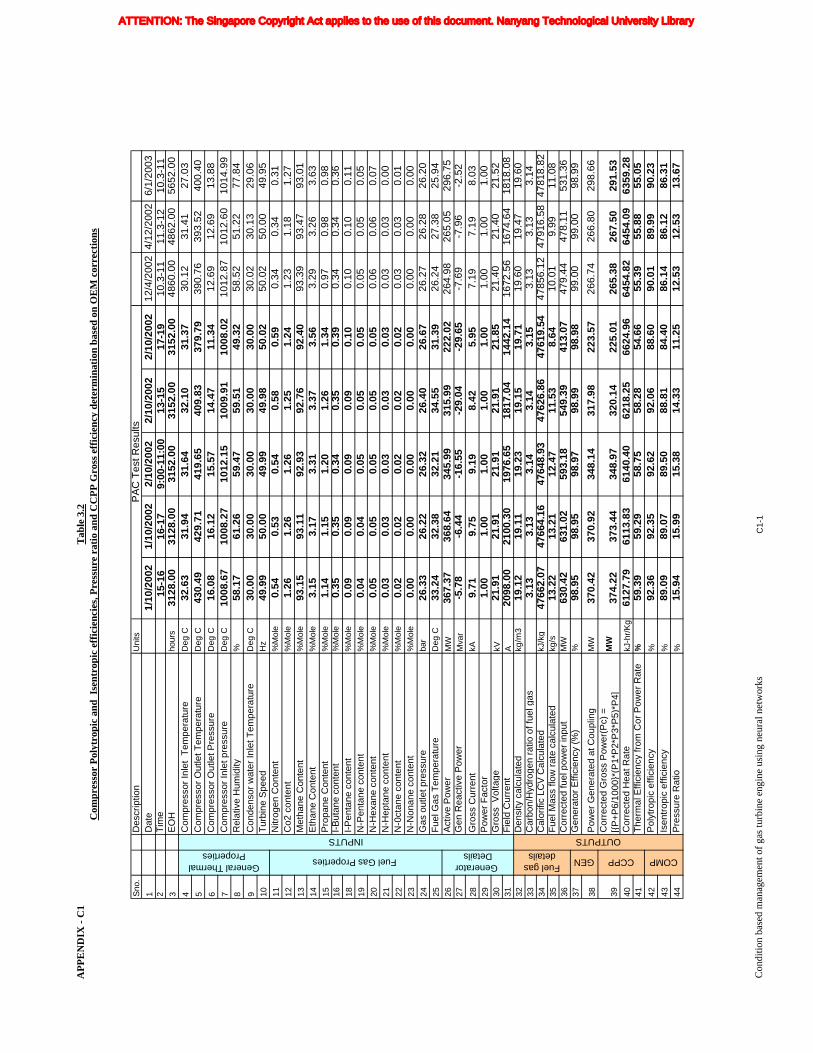
AP
PE
ND
IX -
C1
Tab
le 3
.2C
ompr
esso
r P
olyt
ropi
c an
d I
sent
ropi
c ef
fici
enci
es, P
ress
ure
rati
o an
d C
CP
P G
ross
eff
icie
ncy
dete
rmin
atio
n ba
sed
on O
EM
cor
rect
ions
Sno
.D
escr
iptio
nU
nits
1D
ate
1/10
/200
21/
10/2
002
2/10
/200
22/
10/2
002
2/10
/200
212
/4/2
002
4/12
/200
26/
1/20
032
Tim
e
15-1
616
-17
9:00
-11:
0013
-15
17-1
910
.3-1
111
.3-1
210
.3-1
13
EO
Hho
urs
3128
.00
3128
.00
3152
.00
3152
.00
3152
.00
4860
.00
4862
.00
5652
.00
4C
ompr
esso
r Inl
et T
empe
ratu
reD
eg C
32.6
331
.94
31.6
432
.10
31.3
730
.12
31.4
127
.03
5C
ompr
esso
r O
utle
t Tem
pera
ture
Deg
C43
0.49
429.
7141
9.65
409.
8337
9.79
390.
7639
3.52
400.
406
Com
pres
sor
Out
let P
ress
ure
Deg
C16
.08
16.1
215
.57
14.4
711
.34
12.6
912
.69
13.8
87
Com
pres
sor
Inle
t pre
ssur
eD
eg C
1008
.67
1008
.27
1012
.15
1009
.91
1008
.02
1012
.87
1012
.60
1014
.99
8R
elat
ive
Hum
idity
%58
.17
61.2
659
.47
59.5
149
.32
58.5
251
.22
77.8
49
Con
dens
or w
ater
Inle
t Tem
pera
ture
Deg
C30
.00
30.0
030
.00
30.0
030
.00
30.0
230
.13
29.0
610
Tur
bine
Spe
edH
z49
.99
50.0
049
.99
49.9
850
.02
50.0
250
.00
49.9
511
Nitr
ogen
Con
tent
%M
ole
0.54
0.53
0.54
0.58
0.59
0.34
0.34
0.31
12C
o2 c
onte
nt%
Mol
e1.
261.
261.
261.
251.
241.
231.
181.
2713
Met
hane
Con
tent
%M
ole
93.1
593
.11
92.9
392
.76
92.4
093
.39
93.4
793
.01
14E
than
e C
onte
nt%
Mol
e3.
153.
173.
313.
373.
563.
293.
263.
6315
Pro
pane
Con
tent
%M
ole
1.14
1.15
1.20
1.26
1.34
0.97
0.98
0.98
16I-
But
ane
cont
ent
%M
ole
0.35
0.35
0.34
0.35
0.39
0.34
0.34
0.36
18I-
Pen
tane
con
tent
%M
ole
0.09
0.09
0.09
0.09
0.10
0.10
0.10
0.11
19N
-Pen
tane
con
tent
%M
ole
0.04
0.04
0.05
0.05
0.05
0.05
0.05
0.05
20N
-Hex
ane
cont
ent
%M
ole
0.05
0.05
0.05
0.05
0.05
0.06
0.06
0.07
21N
-Hep
tane
con
tent
%M
ole
0.03
0.03
0.03
0.03
0.03
0.03
0.03
0.00
22N
-0ct
ane
cont
ent
%M
ole
0.02
0.02
0.02
0.02
0.02
0.03
0.03
0.01
23N
-Non
ane
cont
ent
%M
ole
0.00
0.00
0.00
0.00
0.00
0.00
0.00
0.00
24G
as o
utle
t pre
ssur
eba
r26
.33
26.2
226
.32
26.4
026
.67
26.2
726
.28
26.2
025
Fue
l Gas
Tem
pera
ture
Deg
C33
.24
32.3
832
.21
34.5
531
.39
26.2
427
.38
25.9
426
Act
ive
Pow
erM
W36
7.37
368.
6434
5.99
315.
9922
2.02
264.
9826
5.05
296.
7527
Gen
Rea
ctiv
e P
ower
Mva
r-5
.78
-6.4
4-1
6.55
-29.
04-2
9.65
-7.6
9-7
.96
-2.5
228
Gro
ss C
urre
ntkA
9.71
9.75
9.19
8.42
5.95
7.19
7.19
8.03
29P
ower
Fac
tor
1.00
1.00
1.00
1.00
1.00
1.00
1.00
1.00
30G
ross
Vol
tage
kV21
.91
21.9
121
.91
21.9
121
.85
21.4
021
.40
21.5
231
Fie
ld C
urre
ntA
2098
.00
2100
.30
1976
.65
1817
.04
1442
.14
1672
.56
1674
.64
1818
.08
32D
ensi
ty c
alcu
late
d kg
/m3
19.1
219
.11
19.2
319
.15
19.7
119
.60
19.4
719
.60
33C
arbo
n/H
ydro
gen
ratio
of f
uel g
as
3.13
3.13
3.14
3.14
3.15
3.13
3.13
3.14
34C
alor
ific
LCV
Cal
cula
ted
kJ/k
g47
662.
0747
664.
1647
648.
9347
626.
8647
619.
5447
856.
1247
916.
5847
818.
8235
Fue
l Mas
s flo
w r
ate
calc
ulat
edkg
/s13
.22
13.2
112
.47
11.5
38.
6410
.01
9.99
11.0
836
Cor
rect
ed fu
el p
ower
inpu
tM
W63
0.42
631.
0259
3.18
549.
3941
3.07
479.
4447
8.11
531.
3637
Gen
erat
or E
ffici
ency
(%)
%98
.95
98.9
598
.97
98.9
998
.98
99.0
099
.00
98.9
9
38P
ower
Gen
erat
ed a
t Cou
plin
gM
W37
0.42
370.
9234
8.14
317.
9822
3.57
266.
7426
6.80
298.
66
39C
orre
cted
Gro
ss P
ower
(Pc)
=
[{P
+P6/
1000
}*(P
1*P
2*P
3*P
5)*P
4]M
W37
4.22
373.
4434
8.97
320.
1422
5.01
265.
3826
7.50
291.
5340
Cor
rect
ed H
eat R
ate
kJ-h
r/K
g61
27.7
961
13.8
361
40.4
062
18.2
566
24.9
664
54.8
264
54.0
963
59.2
841
The
rmal
Effi
cien
cy fr
om C
or P
ower
Rat
e%
59.3
959
.29
58.7
558
.28
54.6
655
.39
55.8
855
.05
42P
olyt
ropi
c ef
ficie
ncy
%92
.36
92.3
592
.62
92.0
688
.60
90.0
189
.99
90.2
343
Isen
trop
ic e
ffici
ency
%89
.09
89.0
789
.50
88.8
184
.40
86.1
486
.12
86.3
144
Pre
ssur
e R
atio
%15
.94
15.9
915
.38
14.3
311
.25
12.5
312
.53
13.6
7
COMP
OUTPUTS
PA
C T
est R
esul
ts
Fuel gas details
GEN CCPP
INPUTS
General Thermal Properties
Fuel Gas Properties Generator
Details
Con
ditio
n ba
sed
man
agem
ent o
f gas
turb
ine
engi
ne u
sing
neu
ral n
etw
orks
C1-
1
ATTENTION: The Singapore Copyright Act applies to the use of this document. Nanyang Technological University Library
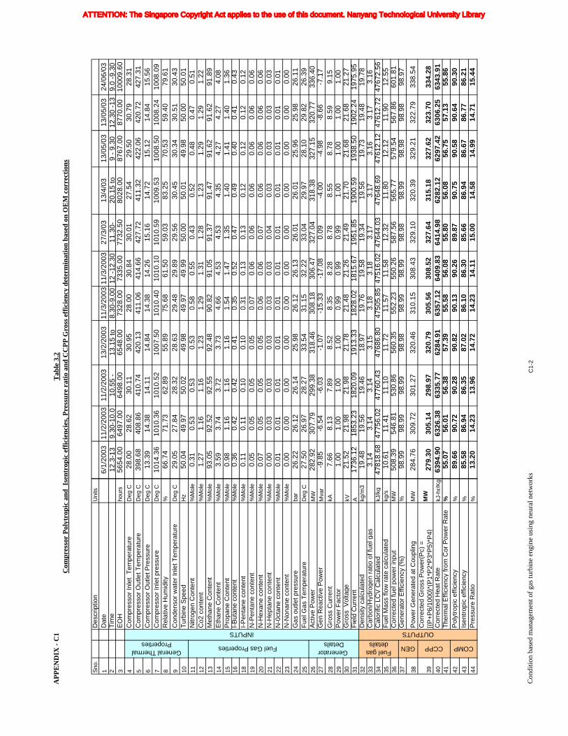
AP
PE
ND
IX -
C1
Tab
le 3
.2C
ompr
esso
r P
olyt
ropi
c an
d I
sent
ropi
c ef
fici
enci
es, P
ress
ure
rati
o an
d C
CP
P G
ross
eff
icie
ncy
dete
rmin
atio
n ba
sed
on O
EM
cor
rect
ions
Sno
.D
escr
iptio
nU
nits
1D
ate
2T
ime
3E
OH
hour
s
4C
ompr
esso
r Inl
et T
empe
ratu
reD
eg C
5C
ompr
esso
r O
utle
t Tem
pera
ture
Deg
C
6C
ompr
esso
r O
utle
t Pre
ssur
eD
eg C
7C
ompr
esso
r In
let p
ress
ure
Deg
C
8R
elat
ive
Hum
idity
%
9C
onde
nsor
wat
er In
let T
empe
ratu
reD
eg C
10T
urbi
ne S
peed
Hz
11N
itrog
en C
onte
nt%
Mol
e
12C
o2 c
onte
nt%
Mol
e
13M
etha
ne C
onte
nt%
Mol
e
14E
than
e C
onte
nt%
Mol
e
15P
ropa
ne C
onte
nt%
Mol
e16
I-B
utan
e co
nten
t%
Mol
e
18I-
Pen
tane
con
tent
%M
ole
19N
-Pen
tane
con
tent
%M
ole
20N
-Hex
ane
cont
ent
%M
ole
21N
-Hep
tane
con
tent
%M
ole
22N
-0ct
ane
cont
ent
%M
ole
23N
-Non
ane
cont
ent
%M
ole
24G
as o
utle
t pre
ssur
eba
r
25F
uel G
as T
empe
ratu
reD
eg C
26A
ctiv
e P
ower
MW
27G
en R
eact
ive
Pow
erM
var
28G
ross
Cur
rent
kA29
Pow
er F
acto
r30
Gro
ss V
olta
gekV
31F
ield
Cur
rent
A32
Den
sity
cal
cula
ted
kg/m
333
Car
bon/
Hyd
roge
n ra
tio o
f fue
l gas
34
Cal
orifi
c LC
V C
alcu
late
dkJ
/kg
35F
uel M
ass
flow
rat
e ca
lcul
ated
kg/s
36C
orre
cted
fuel
pow
er in
put
MW
37G
ener
ator
Effi
cien
cy (%
)%
38P
ower
Gen
erat
ed a
t Cou
plin
gM
W
39C
orre
cted
Gro
ss P
ower
(Pc)
=
[{P
+P6/
1000
}*(P
1*P
2*P
3*P
5)*P
4]M
W
40C
orre
cted
Hea
t Rat
ekJ
-hr/
Kg
41T
herm
al E
ffici
ency
from
Cor
Pow
er R
ate
%
42P
olyt
ropi
c ef
ficie
ncy
%
43Is
entr
opic
effi
cien
cy%
44P
ress
ure
Rat
io%
COMP
OUTPUTS
Fuel gas details
GEN CCPP
INPUTS
General Thermal Properties
Fuel Gas Properties Generator
Details
6/1/
2003
11/2
/200
311
/2/2
003
13/2
/200
311
/3/2
003
11/3
/200
327
/3/0
313
/4/0
313
/05/
0313
/05/
0324
/06/
0312
.3-1
39.
30-1
0.0
10.5
5 -
13.1
5 to
8.
30-9
.00
12 -
12.3
011
.30-
20.1
5 to
9
- 9.
3012
.30
-13
9.0
-9.3
056
54.0
064
97.0
064
98.0
065
48.0
073
28.0
073
35.0
077
32.5
080
28.0
087
67.0
087
70.0
010
009.
6028
.00
28.6
230
.11
30.9
528
.00
30.8
430
.01
27.5
429
.50
30.7
928
.31
398.
6840
8.86
410.
7442
0.13
411.
0641
4.66
427.
7241
1.32
422.
0642
0.72
427.
3113
.39
14.3
814
.11
14.8
414
.38
14.2
615
.16
14.7
215
.12
14.8
415
.56
1014
.36
1010
.36
1010
.52
1007
.50
1010
.40
1010
.10
1010
.59
1009
.53
1008
.50
1008
.24
1008
.09
66.7
471
.73
62.8
955
.89
75.6
861
.50
59.0
383
.25
70.5
359
.40
79.6
129
.05
27.8
428
.32
28.6
329
.48
29.8
929
.56
30.4
530
.34
30.5
130
.43
50.0
449
.97
50.0
249
.98
49.9
749
.99
50.0
050
.01
49.9
850
.00
50.0
10.
310.
530.
530.
530.
580.
550.
430.
520.
480.
470.
511.
271.
161.
161.
231.
291.
311.
281.
231.
291.
291.
2293
.05
92.5
292
.55
92.4
890
.82
91.0
591
.37
91.4
791
.62
91.6
291
.89
3.59
3.74
3.72
3.73
4.66
4.53
4.53
4.35
4.27
4.27
4.08
0.98
1.16
1.16
1.16
1.54
1.47
1.35
1.40
1.41
1.40
1.36
0.36
0.42
0.42
0.41
0.35
0.52
0.47
0.49
0.40
0.41
0.43
0.11
0.11
0.10
0.10
0.31
0.13
0.13
0.12
0.12
0.12
0.12
0.05
0.05
0.05
0.05
0.07
0.06
0.06
0.06
0.06
0.06
0.06
0.07
0.05
0.05
0.05
0.06
0.06
0.07
0.06
0.06
0.06
0.06
0.00
0.03
0.03
0.03
0.03
0.03
0.04
0.03
0.03
0.03
0.03
0.01
0.01
0.01
0.01
0.01
0.01
0.01
0.01
0.01
0.01
0.01
0.00
0.00
0.00
0.00
0.00
0.00
0.00
0.00
0.00
0.00
0.00
26.2
226
.12
26.1
425
.98
26.1
226
.13
26.0
126
.01
25.9
625
.98
26.1
127
.50
26.9
728
.27
33.5
431
.15
32.2
233
.04
29.9
728
.10
29.8
226
.39
282.
9230
7.79
299.
3831
8.46
308.
1830
6.47
327.
0431
8.38
327.
1532
0.77
336.
40-9
.85
-6.5
4-6
.03
-1.0
7-1
5.33
-17.
080.
09-4
.00
-4.9
8-8
.66
-7.1
77.
668.
137.
898.
528.
358.
288.
788.
558.
788.
599.
151.
001.
001.
001.
000.
990.
990.
991.
001.
001.
001.
0021
.52
21.9
821
.98
21.7
821
.48
21.2
621
.49
21.7
021
.68
21.6
821
.27
1736
.12
1853
.23
1820
.09
1913
.33
1828
.02
1815
.67
1951
.85
1900
.59
1938
.50
1902
.24
1975
.95
19.4
819
.56
19.4
618
.97
19.7
619
.58
19.3
419
.56
19.7
319
.48
19.7
83.
143.
143.
143.
153.
183.
183.
173.
173.
163.
173.
1647
818.
6847
756.
0247
760.
4347
686.
8047
505.
8547
516.
0247
644.
0347
648.
6947
612.
1247
612.
7247
672.
5610
.61
11.4
111
.10
11.7
211
.57
11.5
812
.32
11.8
012
.12
11.9
012
.55
508.
3954
6.81
530.
8656
0.35
552.
2355
0.26
587.
5656
5.77
579.
5456
7.86
601.
8198
.99
98.9
998
.99
98.9
898
.99
98.9
998
.98
98.9
998
.98
98.9
898
.97
284.
7630
9.72
301.
2732
0.46
310.
1530
8.43
329.
1032
0.39
329.
2132
2.79
338.
54
279.
3030
5.14
298.
9732
0.79
305.
5630
8.52
327.
6431
5.18
327.
6232
3.70
334.
2863
94.9
063
26.3
863
35.7
762
84.9
163
57.1
264
09.8
364
14.9
862
82.1
262
97.4
263
06.2
563
43.9
155
.07
56.0
156
.38
57.3
955
.58
56.0
855
.80
56.0
856
.75
57.1
355
.86
89.6
690
.72
90.2
890
.82
90.1
390
.26
89.8
790
.75
90.5
890
.64
90.3
085
.58
86.9
486
.35
87.0
286
.10
86.3
085
.66
86.9
486
.67
86.7
786
.21
13.2
014
.23
13.9
614
.72
14.2
314
.11
15.0
014
.58
14.9
914
.71
15.4
4
Con
ditio
n ba
sed
man
agem
ent o
f gas
turb
ine
engi
ne u
sing
neu
ral n
etw
orks
C1-
2
ATTENTION: The Singapore Copyright Act applies to the use of this document. Nanyang Technological University Library
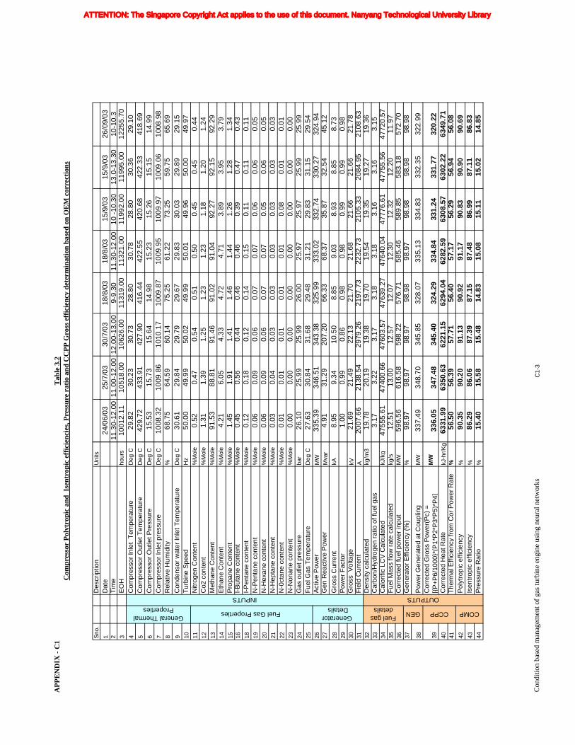
AP
PE
ND
IX -
C1
Tab
le 3
.2C
ompr
esso
r P
olyt
ropi
c an
d I
sent
ropi
c ef
fici
enci
es, P
ress
ure
rati
o an
d C
CP
P G
ross
eff
icie
ncy
dete
rmin
atio
n ba
sed
on O
EM
cor
rect
ions
Sno
.D
escr
iptio
nU
nits
1D
ate
2T
ime
3E
OH
hour
s
4C
ompr
esso
r Inl
et T
empe
ratu
reD
eg C
5C
ompr
esso
r O
utle
t Tem
pera
ture
Deg
C
6C
ompr
esso
r O
utle
t Pre
ssur
eD
eg C
7C
ompr
esso
r In
let p
ress
ure
Deg
C
8R
elat
ive
Hum
idity
%
9C
onde
nsor
wat
er In
let T
empe
ratu
reD
eg C
10T
urbi
ne S
peed
Hz
11N
itrog
en C
onte
nt%
Mol
e
12C
o2 c
onte
nt%
Mol
e
13M
etha
ne C
onte
nt%
Mol
e
14E
than
e C
onte
nt%
Mol
e
15P
ropa
ne C
onte
nt%
Mol
e16
I-B
utan
e co
nten
t%
Mol
e
18I-
Pen
tane
con
tent
%M
ole
19N
-Pen
tane
con
tent
%M
ole
20N
-Hex
ane
cont
ent
%M
ole
21N
-Hep
tane
con
tent
%M
ole
22N
-0ct
ane
cont
ent
%M
ole
23N
-Non
ane
cont
ent
%M
ole
24G
as o
utle
t pre
ssur
eba
r
25F
uel G
as T
empe
ratu
reD
eg C
26A
ctiv
e P
ower
MW
27G
en R
eact
ive
Pow
erM
var
28G
ross
Cur
rent
kA29
Pow
er F
acto
r30
Gro
ss V
olta
gekV
31F
ield
Cur
rent
A32
Den
sity
cal
cula
ted
kg/m
333
Car
bon/
Hyd
roge
n ra
tio o
f fue
l gas
34
Cal
orifi
c LC
V C
alcu
late
dkJ
/kg
35F
uel M
ass
flow
rat
e ca
lcul
ated
kg/s
36C
orre
cted
fuel
pow
er in
put
MW
37G
ener
ator
Effi
cien
cy (%
)%
38P
ower
Gen
erat
ed a
t Cou
plin
gM
W
39C
orre
cted
Gro
ss P
ower
(Pc)
=
[{P
+P6/
1000
}*(P
1*P
2*P
3*P
5)*P
4]M
W
40C
orre
cted
Hea
t Rat
ekJ
-hr/
Kg
41T
herm
al E
ffici
ency
from
Cor
Pow
er R
ate
%
42P
olyt
ropi
c ef
ficie
ncy
%
43Is
entr
opic
effi
cien
cy%
44P
ress
ure
Rat
io%
COMP
OUTPUTS
Fuel gas details
GEN CCPP
INPUTS
General Thermal Properties
Fuel Gas Properties Generator
Details
24/0
6/03
25/7
/03
30/7
/03
18/8
/03
18/8
/03
15/9
/03
15/9
/03
26/0
9/03
11.3
0-12
.00
11.0
0-12
.00
12.0
0-13
.00
9-9.
3011
.30-
12.0
010
-10
.30
13.0
-13.
3010
-10.
310
012.
1110
518.
0010
626.
0011
319.
0011
321.
0011
992.
0011
995.
0012
255.
7029
.82
30.2
330
.73
28.8
030
.78
28.8
030
.36
29.1
042
9.72
433.
9142
7.90
416.
4442
2.55
420.
6842
2.33
418.
6915
.53
15.7
315
.64
14.9
815
.23
15.2
615
.15
14.9
910
08.3
210
09.8
610
10.1
710
09.8
710
09.9
510
09.9
710
09.0
610
08.9
868
.75
64.5
960
.14
75.2
561
.22
73.2
559
.75
65.6
930
.61
29.8
429
.79
29.6
729
.83
30.0
329
.89
29.1
550
.00
49.9
950
.02
49.9
950
.01
49.9
650
.00
49.9
70.
520.
470.
540.
510.
500.
450.
450.
441.
311.
391.
251.
231.
231.
181.
201.
2491
.53
88.8
191
.46
91.0
291
.04
92.2
792
.15
92.2
94.
216.
054.
334.
724.
713.
893.
953.
791.
451.
911.
411.
461.
441.
261.
281.
340.
450.
560.
440.
460.
460.
390.
470.
430.
120.
180.
120.
140.
150.
110.
110.
110.
060.
090.
060.
070.
070.
060.
060.
050.
060.
090.
060.
070.
070.
050.
060.
050.
030.
040.
030.
030.
030.
030.
030.
030.
010.
010.
010.
010.
010.
080.
010.
010.
000.
000.
000.
000.
000.
000.
000.
0026
.10
25.9
925
.99
26.0
025
.97
25.9
725
.99
25.9
927
.63
30.8
431
.68
29.4
831
.21
29.8
331
.15
29.5
433
5.39
346.
5134
3.38
325.
9933
3.02
332.
7433
0.27
324.
944.
9131
.29
207.
2066
.33
68.3
735
.87
32.5
445
.12
8.95
9.34
10.5
08.
859.
038.
938.
858.
731.
000.
990.
860.
980.
980.
990.
990.
9821
.69
21.4
922
.13
21.7
021
.68
21.6
621
.66
21.7
820
07.6
621
38.5
429
79.2
621
97.7
322
32.7
321
05.3
320
84.9
521
08.6
319
.78
20.1
919
.38
19.7
019
.54
19.3
519
.27
19.3
63.
173.
223.
173.
183.
183.
163.
163.
1547
555.
6147
400.
6647
603.
5747
639.
2747
640.
0447
776.
6147
755.
5647
720.
5712
.51
13.0
012
.57
12.0
712
.30
12.3
212
.20
11.9
759
6.56
616.
5859
8.22
576.
7158
5.46
589.
8558
3.18
572.
7098
.97
98.9
798
.97
98.9
898
.97
98.9
898
.98
98.9
8
337.
4934
8.70
345.
8532
8.07
335.
1333
4.83
332.
3532
2.99
336.
0534
7.48
345.
4032
4.29
334.
8433
1.24
331.
7732
0.22
6331
.99
6350
.63
6221
.15
6294
.04
6282
.59
6308
.57
6302
.22
6349
.71
56.5
056
.39
57.7
156
.40
57.1
756
.29
56.9
456
.08
90.3
590
.20
91.1
390
.92
91.1
790
.83
90.9
090
.69
86.2
986
.06
87.3
987
.15
87.4
886
.99
87.1
186
.83
15.4
015
.58
15.4
814
.83
15.0
815
.11
15.0
214
.85
Con
ditio
n ba
sed
man
agem
ent o
f gas
turb
ine
engi
ne u
sing
neu
ral n
etw
orks
C1-
3
ATTENTION: The Singapore Copyright Act applies to the use of this document. Nanyang Technological University Library
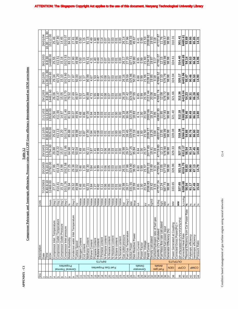
AP
PE
ND
IX -
C1
Tab
le 3
.2C
ompr
esso
r P
olyt
ropi
c an
d I
sent
ropi
c ef
fici
enci
es, P
ress
ure
rati
o an
d C
CP
P G
ross
eff
icie
ncy
dete
rmin
atio
n ba
sed
on O
EM
cor
rect
ions
Sno
.D
escr
iptio
nU
nits
1D
ate
2T
ime
3E
OH
hour
s
4C
ompr
esso
r Inl
et T
empe
ratu
reD
eg C
5C
ompr
esso
r O
utle
t Tem
pera
ture
Deg
C
6C
ompr
esso
r O
utle
t Pre
ssur
eD
eg C
7C
ompr
esso
r In
let p
ress
ure
Deg
C
8R
elat
ive
Hum
idity
%
9C
onde
nsor
wat
er In
let T
empe
ratu
reD
eg C
10T
urbi
ne S
peed
Hz
11N
itrog
en C
onte
nt%
Mol
e
12C
o2 c
onte
nt%
Mol
e
13M
etha
ne C
onte
nt%
Mol
e
14E
than
e C
onte
nt%
Mol
e
15P
ropa
ne C
onte
nt%
Mol
e16
I-B
utan
e co
nten
t%
Mol
e
18I-
Pen
tane
con
tent
%M
ole
19N
-Pen
tane
con
tent
%M
ole
20N
-Hex
ane
cont
ent
%M
ole
21N
-Hep
tane
con
tent
%M
ole
22N
-0ct
ane
cont
ent
%M
ole
23N
-Non
ane
cont
ent
%M
ole
24G
as o
utle
t pre
ssur
eba
r
25F
uel G
as T
empe
ratu
reD
eg C
26A
ctiv
e P
ower
MW
27G
en R
eact
ive
Pow
erM
var
28G
ross
Cur
rent
kA29
Pow
er F
acto
r30
Gro
ss V
olta
gekV
31F
ield
Cur
rent
A32
Den
sity
cal
cula
ted
kg/m
333
Car
bon/
Hyd
roge
n ra
tio o
f fue
l gas
34
Cal
orifi
c LC
V C
alcu
late
dkJ
/kg
35F
uel M
ass
flow
rat
e ca
lcul
ated
kg/s
36C
orre
cted
fuel
pow
er in
put
MW
37G
ener
ator
Effi
cien
cy (%
)%
38P
ower
Gen
erat
ed a
t Cou
plin
gM
W
39C
orre
cted
Gro
ss P
ower
(Pc)
=
[{P
+P6/
1000
}*(P
1*P
2*P
3*P
5)*P
4]M
W
40C
orre
cted
Hea
t Rat
ekJ
-hr/
Kg
41T
herm
al E
ffici
ency
from
Cor
Pow
er R
ate
%
42P
olyt
ropi
c ef
ficie
ncy
%
43Is
entr
opic
effi
cien
cy%
44P
ress
ure
Rat
io%
COMP
OUTPUTS
Fuel gas details
GEN CCPP
INPUTS
General Thermal Properties
Fuel Gas Properties Generator
Details7/
10/2
003
20/1
0/03
20/1
0/03
21/1
1/03
21/1
1/03
29/1
2/03
29/1
2/03
30/1
2/03
26/0
1/04
8.40
-9.1
09.
3-10
.011
.3-1
2.0
8:00
-8:3
013
-13:
308-
8:30
11.0
0-11
.30
8-8:
3010
.30
- 11
.30
1246
9.00
1279
2.00
1279
4.00
1352
6.00
1353
0.00
1446
1.60
1446
4.60
1448
8.00
1511
2.00
27.3
727
.96
29.8
825
.62
25.5
626
.06
29.3
425
.55
25.4
641
4.41
414.
1841
8.22
413.
1341
1.66
414.
4742
1.20
413.
5140
7.80
15.1
914
.98
15.0
715
.20
14.9
715
.05
15.1
015
.16
14.4
510
11.2
610
12.5
810
11.9
510
11.6
210
11.4
010
13.7
010
13.6
010
13.5
310
10.0
778
.94
77.2
564
.98
85.8
881
.93
79.5
261
.17
83.1
284
.91
29.5
229
.38
29.4
230
.01
30.0
727
.69
27.8
727
.80
27.8
149
.98
50.0
250
.04
49.9
849
.95
49.9
750
.00
49.9
949
.96
0.46
0.46
0.49
0.51
0.48
0.52
0.51
0.50
0.50
1.20
1.20
1.20
0.87
0.86
1.17
1.17
1.13
1.15
92.3
192
.30
92.1
197
.00
97.0
090
.88
90.9
991
.61
91.1
53.
843.
843.
870.
940.
944.
734.
674.
314.
491.
271.
311.
410.
430.
441.
551.
531.
401.
600.
420.
390.
390.
180.
180.
480.
470.
440.
460.
110.
110.
120.
030.
030.
150.
150.
140.
140.
060.
060.
060.
010.
010.
080.
080.
070.
070.
050.
050.
060.
010.
010.
070.
070.
070.
070.
030.
030.
030.
010.
010.
030.
030.
030.
030.
010.
010.
010.
000.
000.
010.
010.
010.
010.
000.
000.
000.
000.
000.
000.
000.
000.
0025
.98
26.0
125
.98
26.1
526
.18
26.1
826
.16
26.1
726
.14
28.2
727
.98
29.3
728
.45
30.0
627
.42
29.5
927
.20
27.9
633
1.55
324.
9032
7.25
329.
0032
3.35
324.
5932
5.96
327.
5130
8.33
18.5
936
.55
35.8
423
.16
18.8
347
.55
50.2
050
.80
45.6
78.
958.
808.
848.
888.
748.
858.
888.
958.
411.
000.
991.
001.
001.
000.
990.
990.
990.
9921
.54
21.5
721
.57
21.5
021
.50
21.5
621
.56
21.6
021
.53
2036
.83
2070
.22
2077
.83
2039
.27
2002
.66
2111
.44
2128
.12
2134
.52
2038
.60
19.4
219
.49
19.4
118
.25
18.1
620
.08
19.8
519
.87
19.9
33.
153.
153.
163.
043.
053.
183.
183.
173.
1847
757.
2447
759.
0047
719.
8048
337.
8348
362.
3047
691.
7447
696.
5247
781.
0747
727.
8712
.24
12.0
512
.13
12.0
511
.85
12.0
812
.10
12.1
511
.76
587.
7357
7.02
578.
9058
6.99
577.
8357
8.72
576.
7958
3.98
566.
5798
.98
98.9
898
.98
98.9
898
.98
98.9
898
.98
98.9
898
.99
333.
6532
6.96
329.
3332
8.08
321.
4032
1.66
324.
0432
4.61
310.
31
327.
6532
1.16
327.
1531
8.38
312.
1831
2.36
320.
1731
4.40
301.
4162
85.6
863
16.7
063
12.1
763
66.0
363
82.6
864
19.0
464
03.9
664
08.6
964
85.6
156
.04
55.8
356
.54
54.6
654
.46
54.2
355
.47
54.1
453
.69
91.1
790
.90
91.1
490
.76
90.4
990
.31
90.4
690
.53
89.9
587
.49
87.1
387
.45
86.9
086
.55
86.2
886
.50
86.5
885
.85
15.0
214
.79
14.8
915
.02
14.8
014
.85
14.9
014
.96
14.3
1
Con
ditio
n ba
sed
man
agem
ent o
f gas
turb
ine
engi
ne u
sing
neu
ral n
etw
orks
C1-
4
ATTENTION: The Singapore Copyright Act applies to the use of this document. Nanyang Technological University Library
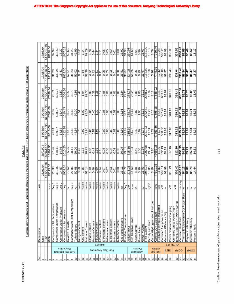
AP
PE
ND
IX -
C1
Tab
le 3
.2C
ompr
esso
r P
olyt
ropi
c an
d I
sent
ropi
c ef
fici
enci
es, P
ress
ure
rati
o an
d C
CP
P G
ross
eff
icie
ncy
dete
rmin
atio
n ba
sed
on O
EM
cor
rect
ions
Sno
.D
escr
iptio
nU
nits
1D
ate
2T
ime
3E
OH
hour
s
4C
ompr
esso
r Inl
et T
empe
ratu
reD
eg C
5C
ompr
esso
r O
utle
t Tem
pera
ture
Deg
C
6C
ompr
esso
r O
utle
t Pre
ssur
eD
eg C
7C
ompr
esso
r In
let p
ress
ure
Deg
C
8R
elat
ive
Hum
idity
%
9C
onde
nsor
wat
er In
let T
empe
ratu
reD
eg C
10T
urbi
ne S
peed
Hz
11N
itrog
en C
onte
nt%
Mol
e
12C
o2 c
onte
nt%
Mol
e
13M
etha
ne C
onte
nt%
Mol
e
14E
than
e C
onte
nt%
Mol
e
15P
ropa
ne C
onte
nt%
Mol
e16
I-B
utan
e co
nten
t%
Mol
e
18I-
Pen
tane
con
tent
%M
ole
19N
-Pen
tane
con
tent
%M
ole
20N
-Hex
ane
cont
ent
%M
ole
21N
-Hep
tane
con
tent
%M
ole
22N
-0ct
ane
cont
ent
%M
ole
23N
-Non
ane
cont
ent
%M
ole
24G
as o
utle
t pre
ssur
eba
r
25F
uel G
as T
empe
ratu
reD
eg C
26A
ctiv
e P
ower
MW
27G
en R
eact
ive
Pow
erM
var
28G
ross
Cur
rent
kA29
Pow
er F
acto
r30
Gro
ss V
olta
gekV
31F
ield
Cur
rent
A32
Den
sity
cal
cula
ted
kg/m
333
Car
bon/
Hyd
roge
n ra
tio o
f fue
l gas
34
Cal
orifi
c LC
V C
alcu
late
dkJ
/kg
35F
uel M
ass
flow
rat
e ca
lcul
ated
kg/s
36C
orre
cted
fuel
pow
er in
put
MW
37G
ener
ator
Effi
cien
cy (%
)%
38P
ower
Gen
erat
ed a
t Cou
plin
gM
W
39C
orre
cted
Gro
ss P
ower
(Pc)
=
[{P
+P6/
1000
}*(P
1*P
2*P
3*P
5)*P
4]M
W
40C
orre
cted
Hea
t Rat
ekJ
-hr/
Kg
41T
herm
al E
ffici
ency
from
Cor
Pow
er R
ate
%
42P
olyt
ropi
c ef
ficie
ncy
%
43Is
entr
opic
effi
cien
cy%
44P
ress
ure
Rat
io%
COMP
OUTPUTS
Fuel gas details
GEN CCPP
INPUTS
General Thermal Properties
Fuel Gas Properties Generator
Details
26/0
1/04
28/0
2/04
14/0
3/04
21/0
4/04
22/0
4/04
17/0
5/04
17/0
5/04
12.0
0-12
.30
10.0
0-10
.30
10.0
0-10
.30
10.0
0-10
.30
15.3
0-16
.30
10.0
0-10
.30
14.0
0-14
.30
1511
3.00
1599
7.50
1651
0.00
1756
1.00
1758
9.64
1818
4.00
1818
8.00
26.3
327
.96
28.9
430
.39
28.7
431
.23
32.9
941
2.02
418.
4140
9.97
428.
2742
5.25
430.
2643
2.50
14.5
714
.76
14.5
615
.49
15.5
015
.41
15.2
710
09.0
410
10.2
010
12.2
810
10.4
310
04.6
610
09.3
010
07.1
879
.62
65.2
667
.13
60.7
968
.55
67.5
159
.66
27.8
628
.41
28.8
330
.43
30.7
031
.23
31.2
650
.08
50.0
049
.97
50.0
049
.98
50.0
249
.99
0.50
0.49
0.75
0.51
0.49
0.52
0.52
1.15
1.18
0.97
1.02
1.04
1.14
1.14
91.1
490
.75
89.9
592
.37
92.3
092
.39
92.2
94.
494.
855.
053.
843.
933.
723.
780.
460.
480.
570.
400.
390.
420.
441.
601.
551.
971.
301.
291.
311.
340.
140.
150.
150.
120.
120.
110.
110.
070.
080.
090.
060.
060.
050.
050.
070.
080.
060.
060.
060.
050.
050.
030.
030.
020.
020.
030.
030.
020.
010.
010.
010.
010.
010.
010.
010.
000.
000.
000.
000.
000.
000.
0026
.11
26.0
925
.99
25.9
125
.94
25.9
125
.92
28.7
229
.51
29.9
230
.15
29.2
030
.67
31.9
331
1.21
315.
1631
5.19
338.
0533
8.73
334.
3633
0.98
44.5
027
.94
44.7
519
.67
23.2
858
.25
51.5
88.
488.
498.
428.
878.
899.
068.
940.
991.
000.
991.
001.
000.
990.
9921
.53
21.5
921
.79
22.1
522
.15
21.6
721
.67
2042
.36
2002
.68
2061
.83
2062
.61
2078
.77
2188
.99
2151
.09
19.8
519
.84
19.9
419
.22
19.3
219
.18
19.1
33.
193.
203.
223.
163.
163.
163.
7647
691.
2547
656.
3847
663.
8647
898.
1847
888.
0247
749.
9147
750.
4611
.83
11.9
611
.74
12.4
712
.49
12.4
212
.28
569.
1157
2.19
560.
5859
7.70
603.
8059
3.06
586.
2098
.99
98.9
998
.99
98.9
798
.97
98.9
798
.98
313.
2131
7.16
317.
1834
0.13
340.
8233
6.48
333.
08
305.
4031
2.26
313.
6233
9.62
339.
4533
7.04
337.
5564
60.7
064
51.9
563
35.7
563
11.3
663
07.5
663
33.4
363
36.4
354
.13
54.8
056
.05
56.8
656
.73
56.8
457
.55
89.8
889
.79
91.0
290
.64
90.7
590
.47
90.4
985
.73
85.5
987
.34
86.7
186
.85
86.4
786
.52
14.4
414
.61
14.3
915
.33
15.4
215
.27
15.1
7
Con
ditio
n ba
sed
man
agem
ent o
f gas
turb
ine
engi
ne u
sing
neu
ral n
etw
orks
C1-
5
ATTENTION: The Singapore Copyright Act applies to the use of this document. Nanyang Technological University Library
AP
PE
ND
IX-C
2T
able
3.3
Com
pres
sor
Pol
ytro
pic,
Ise
ntro
pic
effi
cien
cies
, Pre
ssur
e r
atio
and
CC
PP
Gro
ss e
ffic
ienc
y de
term
inat
ion
usin
g ST
D C
orre
ctio
ns
Sno
.D
escr
iptio
nU
nits
1D
ate
1/10
/200
21/
10/2
002
2/10
/200
22/
10/2
002
2/10
/200
212
/4/2
002
4/12
/200
22
Tim
e
15-1
616
-17
9:00
-11:
0013
-15
17-1
910
.3-1
111
.3-1
23
EO
Hho
urs
3128
.00
3128
.00
3152
.00
3152
.00
3152
.00
4860
.00
4862
.00
4C
ompr
esso
r In
let
Tem
pera
ture
Deg
C32
.63
31.9
431
.64
32.1
031
.37
30.1
231
.41
5C
ompr
esso
r O
utle
t Tem
pera
ture
Deg
C43
0.49
429.
7141
9.65
409.
8337
9.79
390.
7639
3.52
6C
ompr
esso
r O
utle
t Pre
ssur
eD
eg C
16.0
816
.12
15.5
714
.47
11.3
412
.69
12.6
97
Am
bien
t Pre
ssur
eD
eg C
1009
.77
1009
.38
1013
.22
1010
.89
1008
.78
1013
.62
1013
.35
8C
onde
nsor
wat
er In
let T
empe
ratu
reD
eg C
30.0
030
.00
30.0
030
.00
30.0
030
.02
30.1
39
Tur
bine
Spe
edH
z49
.99
50.0
049
.99
49.9
850
.02
50.0
250
.00
10N
itrog
en C
onte
nt%
Mol
e0.
540.
530.
540.
580.
590.
340.
3411
Co2
con
tent
%M
ole
1.26
1.26
1.26
1.25
1.24
1.23
1.18
12M
etha
ne C
onte
nt%
Mol
e93
.15
93.1
192
.93
92.7
692
.40
93.3
993
.47
13E
than
e C
onte
nt%
Mol
e3.
153.
173.
313.
373.
563.
293.
2614
Pro
pane
Con
tent
%M
ole
1.14
1.15
1.20
1.26
1.34
0.97
0.98
15I-
But
ane
cont
ent
%M
ole
0.35
0.35
0.34
0.35
0.39
0.34
0.34
16N
-But
ane
cont
ent
%M
ole
0.19
0.20
0.18
0.20
0.24
0.18
0.18
17I-
Pen
tane
con
tent
%M
ole
0.09
0.09
0.09
0.09
0.10
0.10
0.10
18N
-Pen
tane
con
tent
%M
ole
0.04
0.04
0.05
0.05
0.05
0.05
0.05
19N
-Hex
ane
cont
ent
%M
ole
0.05
0.05
0.05
0.05
0.05
0.06
0.06
20N
-Hep
tane
con
tent
%M
ole
0.03
0.03
0.03
0.03
0.03
0.03
0.03
21N
-0ct
ane
cont
ent
%M
ole
0.02
0.02
0.02
0.02
0.02
0.03
0.03
22N
-Non
ane
cont
ent
%M
ole
0.00
0.00
0.00
0.00
0.00
0.00
0.00
23G
as o
utle
t pre
ssur
eba
r26
.33
26.2
226
.32
26.4
026
.67
26.2
726
.28
24F
uel G
as T
empe
ratu
reD
eg C
33.2
432
.38
32.2
134
.55
31.3
926
.24
27.3
825
Act
ive
Pow
erM
W36
7.37
368.
6434
5.99
315.
9922
2.02
264.
9826
5.05
26G
en R
eact
ive
Pow
erM
var
-5.7
8-6
.44
-16.
55-2
9.04
-29.
65-7
.69
-7.9
627
Gro
ss C
urre
ntkA
9.71
9.75
9.19
8.42
5.95
7.19
7.19
28P
ower
Fac
tor
1.00
1.00
1.00
1.00
1.00
1.00
1.00
29G
ross
Vol
tage
kV21
.91
21.9
121
.91
21.9
121
.85
21.4
021
.40
30F
ield
Cur
rent
A20
98.0
021
00.3
019
76.6
518
17.0
414
42.1
416
72.5
616
74.6
431
Den
sity
cal
cula
ted
kg/m
319
.12
19.1
119
.23
19.1
519
.71
19.6
019
.47
32C
arbo
n/H
ydro
gen
ratio
of f
uel g
as
3.13
3.13
3.14
3.14
3.15
3.13
3.13
33C
alor
ific
LCV
Cal
cula
ted
kJ/k
g47
662.
0747
664.
1647
648.
9347
626.
8647
619.
5447
856.
1247
916.
5834
Fue
l Mas
s flo
w r
ate
calc
ulat
edkg
/s13
.22
13.2
112
.47
11.5
38.
6410
.01
9.99
35C
orre
cted
fuel
pow
er in
put
MW
630.
4263
1.02
593.
1854
9.39
413.
0747
9.44
478.
1136
Gen
erat
or E
ffici
ency
(%
)%
98.9
598
.95
98.9
798
.99
98.9
899
.00
99.0
037
Pow
er G
ener
ated
at C
oupl
ing
MW
370.
4237
0.92
348.
1431
7.98
223.
5726
6.74
266.
8038
Cor
rect
ed G
ross
Pow
er O
utpu
tM
W37
1.31
372.
3834
8.36
318.
6722
4.79
267.
4826
7.09
39C
orre
cted
Hea
t Rat
ekJ
-hr/
Kg
6112
.09
6100
.43
6140
.40
6218
.25
6624
.96
6454
.82
6454
.09
40T
herm
al E
ffici
ency
from
Cor
Pow
er
%58
.90
59.0
158
.73
58.0
054
.42
55.7
955
.86
41P
olyt
ropi
c ef
ficie
ncy
%92
.36
92.3
592
.62
92.0
688
.60
90.0
189
.99
42Is
entr
opic
effi
cien
cy%
89.0
989
.07
89.5
088
.81
84.4
086
.14
86.1
243
Pre
ssur
e R
atio
%15
.94
15.9
915
.38
14.3
311
.25
12.5
312
.53
Fuel gas details
OUTPUTS
Gen CCPP Comp
PA
C T
est
Res
ult
s
General Thermal
Properties
INPUTS
Fuel Gas Properties Generator
Details
Con
ditio
n ba
sed
man
agem
ent o
f gas
turb
ine
engi
ne u
sing
neu
ral n
etw
orks
C2-
1
ATTENTION: The Singapore Copyright Act applies to the use of this document. Nanyang Technological University Library
AP
PE
ND
IX-C
2T
able
3.3
Com
pres
sor
Pol
ytro
pic,
Ise
ntro
pic
effi
cien
cies
, Pre
ssur
e r
atio
and
CC
PP
Gro
ss e
ffic
ienc
y de
term
inat
ion
usin
g ST
D C
orre
ctio
ns
Sno
.D
escr
iptio
nU
nits
1D
ate
2T
ime
3E
OH
hour
s4
Com
pres
sor
Inle
t T
empe
ratu
reD
eg C
5C
ompr
esso
r O
utle
t Tem
pera
ture
Deg
C6
Com
pres
sor
Out
let P
ress
ure
Deg
C7
Am
bien
t Pre
ssur
eD
eg C
8C
onde
nsor
wat
er In
let T
empe
ratu
reD
eg C
9T
urbi
ne S
peed
Hz
10N
itrog
en C
onte
nt%
Mol
e11
Co2
con
tent
%M
ole
12M
etha
ne C
onte
nt%
Mol
e13
Eth
ane
Con
tent
%M
ole
14P
ropa
ne C
onte
nt%
Mol
e15
I-B
utan
e co
nten
t%
Mol
e16
N-B
utan
e co
nten
t%
Mol
e17
I-P
enta
ne c
onte
nt%
Mol
e18
N-P
enta
ne c
onte
nt%
Mol
e19
N-H
exan
e co
nten
t%
Mol
e20
N-H
epta
ne c
onte
nt%
Mol
e21
N-0
ctan
e co
nten
t%
Mol
e22
N-N
onan
e co
nten
t%
Mol
e23
Gas
out
let p
ress
ure
bar
24F
uel G
as T
empe
ratu
reD
eg C
25A
ctiv
e P
ower
MW
26G
en R
eact
ive
Pow
erM
var
27G
ross
Cur
rent
kA28
Pow
er F
acto
r29
Gro
ss V
olta
gekV
30F
ield
Cur
rent
A31
Den
sity
cal
cula
ted
kg/m
332
Car
bon/
Hyd
roge
n ra
tio o
f fue
l gas
33
Cal
orifi
c LC
V C
alcu
late
dkJ
/kg
34F
uel M
ass
flow
rat
e ca
lcul
ated
kg/s
35C
orre
cted
fuel
pow
er in
put
MW
36G
ener
ator
Effi
cien
cy (
%)
%37
Pow
er G
ener
ated
at C
oupl
ing
MW
38C
orre
cted
Gro
ss P
ower
Out
put
MW
39C
orre
cted
Hea
t Rat
ekJ
-hr/
Kg
40T
herm
al E
ffici
ency
from
Cor
Pow
er
%41
Pol
ytro
pic
effic
ienc
y%
42Is
entr
opic
effi
cien
cy%
43P
ress
ure
Rat
io%
Fuel gas details
OUTPUTS
Gen CCPP CompGeneral Thermal
Properties
INPUTS
Fuel Gas Properties Generator
Details
6/1/
2003
6/1/
2003
11/2
/200
311
/2/2
003
13/2
/03
11/3
/200
311
/3/2
003
27/3
/03
13/4
/03
10.3
-11
12.3
-13
9.30
-10.
010
.55
- 13
.15
to
8.30
-9.0
012
-12
.30
11.3
0-12
.00
20.1
5 to
22.
3056
52.0
056
54.0
064
97.0
064
98.0
065
48.0
073
28.0
073
35.0
077
32.5
080
28.0
027
.03
28.0
028
.62
30.1
130
.95
28.0
030
.84
30.0
127
.54
400.
4039
8.68
408.
8641
0.74
420.
1341
1.06
414.
6642
7.72
411.
3213
.88
13.3
914
.38
14.1
114
.84
14.3
814
.26
15.1
614
.72
1016
.20
1015
.46
1013
.10
1013
.21
1010
.46
1013
.32
1012
.94
1013
.84
1011
.99
29.0
629
.05
27.8
428
.32
28.6
329
.48
29.8
929
.56
30.4
549
.95
50.0
449
.97
50.0
249
.98
49.9
749
.99
50.0
050
.01
0.31
0.31
0.53
0.53
0.53
0.58
0.55
0.43
0.52
1.27
1.27
1.16
1.16
1.23
1.29
1.31
1.28
1.23
93.0
193
.05
92.5
292
.55
92.4
890
.82
91.0
591
.37
91.4
73.
633.
593.
743.
723.
734.
664.
534.
534.
350.
980.
981.
161.
161.
161.
541.
471.
351.
400.
360.
360.
420.
420.
410.
350.
520.
470.
490.
190.
190.
220.
220.
230.
290.
280.
260.
270.
110.
110.
110.
100.
100.
310.
130.
130.
120.
050.
050.
050.
050.
050.
070.
060.
060.
060.
070.
070.
050.
050.
050.
060.
060.
070.
060.
000.
000.
030.
030.
030.
030.
030.
040.
030.
010.
010.
010.
010.
010.
010.
010.
010.
010.
000.
000.
000.
000.
000.
000.
000.
000.
0026
.20
26.2
226
.12
26.1
425
.98
26.1
226
.13
26.0
126
.01
25.9
427
.50
26.9
728
.27
33.5
431
.15
32.2
233
.04
29.9
729
6.75
282.
9230
7.79
299.
3831
8.46
308.
1830
6.47
327.
0431
8.38
-2.5
2-9
.85
-6.5
4-6
.03
-1.0
7-1
5.33
-17.
080.
09-4
.00
8.03
7.66
8.13
7.89
8.52
8.35
8.28
8.78
8.55
1.00
1.00
1.00
1.00
1.00
0.99
0.99
0.99
1.00
21.5
221
.52
21.9
821
.98
21.7
821
.48
21.2
621
.49
21.7
018
18.0
817
36.1
218
53.2
318
20.0
919
13.3
318
28.0
218
15.6
719
51.8
519
00.5
919
.60
19.4
819
.56
19.4
618
.97
19.7
619
.58
19.3
419
.56
3.14
3.14
3.14
3.14
3.15
3.18
3.18
3.17
3.17
4781
8.82
4781
8.68
4775
6.02
4776
0.43
4768
6.80
4750
5.85
4751
6.02
4764
4.03
4764
8.69
11.0
810
.61
11.4
111
.10
11.7
211
.57
11.5
812
.32
11.8
053
1.36
508.
3954
6.81
530.
8656
0.35
552.
2355
0.26
587.
5656
5.77
98.9
998
.99
98.9
998
.99
98.9
898
.99
98.9
998
.98
98.9
929
8.66
284.
7630
9.72
301.
2732
0.46
310.
1530
8.43
329.
1032
0.39
299.
8728
5.64
310.
7030
1.58
321.
3731
1.97
309.
0732
9.81
323.
3563
59.2
863
94.9
063
26.3
863
35.7
762
84.9
163
57.1
264
09.8
364
14.9
862
82.1
256
.43
56.1
956
.82
56.8
157
.35
56.4
956
.17
56.1
357
.15
90.2
389
.66
90.7
290
.28
90.8
290
.13
90.2
689
.87
90.7
586
.31
85.5
886
.94
86.3
587
.02
86.1
086
.30
85.6
686
.94
13.6
713
.20
14.2
313
.96
14.7
214
.23
14.1
115
.00
14.5
8
Con
ditio
n ba
sed
man
agem
ent o
f gas
turb
ine
engi
ne u
sing
neu
ral n
etw
orks
C2-
2
ATTENTION: The Singapore Copyright Act applies to the use of this document. Nanyang Technological University Library

AP
PE
ND
IX-C
2T
able
3.3
Com
pres
sor
Pol
ytro
pic,
Ise
ntro
pic
effi
cien
cies
, Pre
ssur
e r
atio
and
CC
PP
Gro
ss e
ffic
ienc
y de
term
inat
ion
usin
g ST
D C
orre
ctio
ns
Sno
.D
escr
iptio
nU
nits
1D
ate
2T
ime
3E
OH
hour
s4
Com
pres
sor
Inle
t T
empe
ratu
reD
eg C
5C
ompr
esso
r O
utle
t Tem
pera
ture
Deg
C6
Com
pres
sor
Out
let P
ress
ure
Deg
C7
Am
bien
t Pre
ssur
eD
eg C
8C
onde
nsor
wat
er In
let T
empe
ratu
reD
eg C
9T
urbi
ne S
peed
Hz
10N
itrog
en C
onte
nt%
Mol
e11
Co2
con
tent
%M
ole
12M
etha
ne C
onte
nt%
Mol
e13
Eth
ane
Con
tent
%M
ole
14P
ropa
ne C
onte
nt%
Mol
e15
I-B
utan
e co
nten
t%
Mol
e16
N-B
utan
e co
nten
t%
Mol
e17
I-P
enta
ne c
onte
nt%
Mol
e18
N-P
enta
ne c
onte
nt%
Mol
e19
N-H
exan
e co
nten
t%
Mol
e20
N-H
epta
ne c
onte
nt%
Mol
e21
N-0
ctan
e co
nten
t%
Mol
e22
N-N
onan
e co
nten
t%
Mol
e23
Gas
out
let p
ress
ure
bar
24F
uel G
as T
empe
ratu
reD
eg C
25A
ctiv
e P
ower
MW
26G
en R
eact
ive
Pow
erM
var
27G
ross
Cur
rent
kA28
Pow
er F
acto
r29
Gro
ss V
olta
gekV
30F
ield
Cur
rent
A31
Den
sity
cal
cula
ted
kg/m
332
Car
bon/
Hyd
roge
n ra
tio o
f fue
l gas
33
Cal
orifi
c LC
V C
alcu
late
dkJ
/kg
34F
uel M
ass
flow
rat
e ca
lcul
ated
kg/s
35C
orre
cted
fuel
pow
er in
put
MW
36G
ener
ator
Effi
cien
cy (
%)
%37
Pow
er G
ener
ated
at C
oupl
ing
MW
38C
orre
cted
Gro
ss P
ower
Out
put
MW
39C
orre
cted
Hea
t Rat
ekJ
-hr/
Kg
40T
herm
al E
ffici
ency
from
Cor
Pow
er
%41
Pol
ytro
pic
effic
ienc
y%
42Is
entr
opic
effi
cien
cy%
43P
ress
ure
Rat
io%
Fuel gas details
OUTPUTS
Gen CCPP CompGeneral Thermal
Properties
INPUTS
Fuel Gas Properties Generator
Details13
/05/
0313
/05/
0324
/06/
0324
/06/
0325
/7/0
330
/7/0
318
/8/0
318
/8/0
315
/9/0
39
- 9.
3012
.30
-13
9.0
-9.3
011
.30-
12.0
011
.00-
12.0
012
.00-
13.0
09-
9.30
11.3
0-12
.00
10 -
10.3
087
67.0
087
70.0
010
009.
6010
012.
1110
518.
0010
626.
0011
319.
0011
321.
0011
992.
0029
.50
30.7
928
.31
29.8
230
.23
30.7
328
.80
30.7
828
.80
422.
0642
0.72
427.
3142
9.72
433.
9142
7.90
416.
4442
2.55
420.
6815
.12
14.8
415
.56
15.5
315
.73
15.6
414
.98
15.2
315
.26
1011
.42
1011
.05
1011
.65
1011
.90
1013
.60
1013
.90
1013
.47
1013
.73
1014
.09
30.3
430
.51
30.4
330
.61
29.8
429
.79
29.6
729
.83
30.0
349
.98
50.0
050
.01
50.0
049
.99
50.0
249
.99
50.0
149
.96
0.48
0.47
0.51
0.52
0.47
0.54
0.51
0.50
0.45
1.29
1.29
1.22
1.31
1.39
1.25
1.23
1.23
1.18
91.6
291
.62
91.8
991
.53
88.8
191
.46
91.0
291
.04
92.2
74.
274.
274.
084.
216.
054.
334.
724.
713.
891.
411.
401.
361.
451.
911.
411.
461.
441.
260.
400.
410.
430.
450.
560.
440.
460.
460.
390.
240.
250.
240.
260.
400.
290.
300.
300.
240.
120.
120.
120.
120.
180.
120.
140.
150.
110.
060.
060.
060.
060.
090.
060.
070.
070.
060.
060.
060.
060.
060.
090.
060.
070.
070.
050.
030.
030.
030.
030.
040.
030.
030.
030.
030.
010.
010.
010.
010.
010.
010.
010.
010.
080.
000.
000.
000.
000.
000.
000.
000.
000.
0025
.96
25.9
826
.11
26.1
025
.99
25.9
926
.00
25.9
725
.97
28.1
029
.82
26.3
927
.63
30.8
431
.68
29.4
831
.21
29.8
332
7.15
320.
7733
6.40
335.
3934
6.51
343.
3832
5.99
333.
0233
2.74
-4.9
8-8
.66
-7.1
74.
9131
.29
207.
2066
.33
68.3
735
.87
8.78
8.59
9.15
8.95
9.34
10.5
08.
859.
038.
931.
001.
001.
001.
000.
990.
860.
980.
980.
9921
.68
21.6
821
.27
21.6
921
.49
22.1
321
.70
21.6
821
.66
1938
.50
1902
.24
1975
.95
2007
.66
2138
.54
2979
.26
2197
.73
2232
.73
2105
.33
19.7
319
.48
19.7
819
.78
20.1
919
.38
19.7
019
.54
19.3
53.
163.
173.
163.
173.
223.
173.
183.
183.
1647
612.
1247
612.
7247
672.
5647
555.
6147
400.
6647
603.
5747
639.
2747
640.
0447
776.
6112
.12
11.9
012
.55
12.5
113
.00
12.5
712
.07
12.3
012
.32
579.
5456
7.86
601.
8159
6.56
616.
5859
8.22
576.
7158
5.46
589.
8598
.98
98.9
898
.97
98.9
798
.97
98.9
798
.98
98.9
798
.98
329.
2132
2.79
338.
5433
7.49
348.
7034
5.85
328.
0733
5.13
334.
8333
1.31
324.
3634
1.17
339.
1934
9.59
346.
3432
9.60
335.
6433
6.32
6297
.42
6306
.25
6343
.91
6331
.99
6350
.63
6221
.15
6294
.04
6282
.59
6308
.57
57.1
757
.12
56.6
956
.86
56.7
057
.89
57.1
557
.33
57.0
290
.58
90.6
490
.30
90.3
590
.20
91.1
390
.92
91.1
790
.83
86.6
786
.77
86.2
186
.29
86.0
687
.39
87.1
587
.48
86.9
914
.99
14.7
115
.44
15.4
015
.58
15.4
814
.83
15.0
815
.11
Con
ditio
n ba
sed
man
agem
ent o
f gas
turb
ine
engi
ne u
sing
neu
ral n
etw
orks
C2-
3
ATTENTION: The Singapore Copyright Act applies to the use of this document. Nanyang Technological University Library
AP
PE
ND
IX-C
2T
able
3.3
Com
pres
sor
Pol
ytro
pic,
Ise
ntro
pic
effi
cien
cies
, Pre
ssur
e r
atio
and
CC
PP
Gro
ss e
ffic
ienc
y de
term
inat
ion
usin
g ST
D C
orre
ctio
ns
Sno
.D
escr
iptio
nU
nits
1D
ate
2T
ime
3E
OH
hour
s4
Com
pres
sor
Inle
t T
empe
ratu
reD
eg C
5C
ompr
esso
r O
utle
t Tem
pera
ture
Deg
C6
Com
pres
sor
Out
let P
ress
ure
Deg
C7
Am
bien
t Pre
ssur
eD
eg C
8C
onde
nsor
wat
er In
let T
empe
ratu
reD
eg C
9T
urbi
ne S
peed
Hz
10N
itrog
en C
onte
nt%
Mol
e11
Co2
con
tent
%M
ole
12M
etha
ne C
onte
nt%
Mol
e13
Eth
ane
Con
tent
%M
ole
14P
ropa
ne C
onte
nt%
Mol
e15
I-B
utan
e co
nten
t%
Mol
e16
N-B
utan
e co
nten
t%
Mol
e17
I-P
enta
ne c
onte
nt%
Mol
e18
N-P
enta
ne c
onte
nt%
Mol
e19
N-H
exan
e co
nten
t%
Mol
e20
N-H
epta
ne c
onte
nt%
Mol
e21
N-0
ctan
e co
nten
t%
Mol
e22
N-N
onan
e co
nten
t%
Mol
e23
Gas
out
let p
ress
ure
bar
24F
uel G
as T
empe
ratu
reD
eg C
25A
ctiv
e P
ower
MW
26G
en R
eact
ive
Pow
erM
var
27G
ross
Cur
rent
kA28
Pow
er F
acto
r29
Gro
ss V
olta
gekV
30F
ield
Cur
rent
A31
Den
sity
cal
cula
ted
kg/m
332
Car
bon/
Hyd
roge
n ra
tio o
f fue
l gas
33
Cal
orifi
c LC
V C
alcu
late
dkJ
/kg
34F
uel M
ass
flow
rat
e ca
lcul
ated
kg/s
35C
orre
cted
fuel
pow
er in
put
MW
36G
ener
ator
Effi
cien
cy (
%)
%37
Pow
er G
ener
ated
at C
oupl
ing
MW
38C
orre
cted
Gro
ss P
ower
Out
put
MW
39C
orre
cted
Hea
t Rat
ekJ
-hr/
Kg
40T
herm
al E
ffici
ency
from
Cor
Pow
er
%41
Pol
ytro
pic
effic
ienc
y%
42Is
entr
opic
effi
cien
cy%
43P
ress
ure
Rat
io%
Fuel gas details
OUTPUTS
Gen CCPP CompGeneral Thermal
Properties
INPUTS
Fuel Gas Properties Generator
Details15
/9/0
326
/09/
037/
10/2
003
20/1
0/03
20/1
0/03
21/1
1/03
21/1
1/03
29/1
2/03
29/1
2/03
13.0
-13.
3010
-10.
38.
40-9
.10
9.3-
10.0
11.3
-12.
08:
00-8
:30
13-1
3:30
8-8:
3011
.00-
11.3
011
995.
0012
255.
7012
469.
0012
792.
0012
794.
0013
526.
0013
530.
0014
461.
6014
464.
6030
.36
29.1
027
.37
27.9
629
.88
25.6
225
.56
26.0
629
.34
422.
3341
8.69
414.
4141
4.18
418.
2241
3.13
411.
6641
4.47
421.
2015
.15
14.9
915
.19
14.9
815
.07
15.2
014
.97
15.0
515
.10
1013
.13
1013
.03
1013
.72
1014
.88
1014
.27
1014
.14
1013
.87
1016
.41
1016
.46
29.8
929
.15
29.5
229
.38
29.4
230
.01
30.0
727
.69
27.8
750
.00
49.9
749
.98
50.0
250
.04
49.9
849
.95
49.9
750
.00
0.45
0.44
0.46
0.46
0.49
0.51
0.48
0.52
0.51
1.20
1.24
1.20
1.20
1.20
0.87
0.86
1.17
1.17
92.1
592
.29
92.3
192
.30
92.1
197
.00
97.0
090
.88
90.9
93.
953.
793.
843.
843.
870.
940.
944.
734.
671.
281.
341.
271.
311.
410.
430.
441.
551.
530.
470.
430.
420.
390.
390.
180.
180.
480.
470.
240.
230.
240.
250.
260.
040.
040.
350.
340.
110.
110.
110.
110.
120.
030.
030.
150.
150.
060.
050.
060.
060.
060.
010.
010.
080.
080.
060.
050.
050.
050.
060.
010.
010.
070.
070.
030.
030.
030.
030.
030.
010.
010.
030.
030.
010.
010.
010.
010.
010.
000.
000.
010.
010.
000.
000.
000.
000.
000.
000.
000.
000.
0025
.99
25.9
925
.98
26.0
125
.98
26.1
526
.18
26.1
826
.16
31.1
529
.54
28.2
727
.98
29.3
728
.45
30.0
627
.42
29.5
933
0.27
324.
9433
1.55
324.
9032
7.25
329.
0032
3.35
324.
5932
5.96
32.5
445
.12
18.5
936
.55
35.8
423
.16
18.8
347
.55
50.2
08.
858.
738.
958.
808.
848.
888.
748.
858.
880.
990.
981.
000.
991.
001.
001.
000.
990.
9921
.66
21.7
821
.54
21.5
721
.57
21.5
021
.50
21.5
621
.56
2084
.95
2108
.63
2036
.83
2070
.22
2077
.83
2039
.27
2002
.66
2111
.44
2128
.12
19.2
719
.36
19.4
219
.49
19.4
118
.25
18.1
620
.08
19.8
53.
163.
153.
153.
153.
163.
043.
053.
183.
1847
755.
5647
720.
5747
757.
2447
759.
0047
719.
8048
337.
8348
362.
3047
691.
7447
696.
5212
.20
11.9
712
.24
12.0
512
.13
12.0
511
.85
12.0
812
.10
583.
1857
2.70
587.
7357
7.02
578.
9058
6.99
577.
8357
8.72
576.
7998
.98
98.9
898
.98
98.9
898
.98
98.9
898
.98
98.9
898
.98
332.
3532
2.99
333.
6532
6.96
329.
3332
8.08
321.
4032
1.66
324.
0433
3.28
324.
2733
6.04
328.
3733
0.13
331.
2832
4.68
322.
9832
3.65
6302
.22
6349
.71
6285
.68
6316
.70
6312
.17
6366
.03
6382
.68
6419
.04
6403
.96
57.1
556
.62
57.1
856
.91
57.0
356
.44
56.1
955
.81
56.1
190
.90
90.6
991
.17
90.9
091
.14
90.7
690
.49
90.3
190
.46
87.1
186
.83
87.4
987
.13
87.4
586
.90
86.5
586
.28
86.5
015
.02
14.8
515
.02
14.7
914
.89
15.0
214
.80
14.8
514
.90
Con
ditio
n ba
sed
man
agem
ent o
f gas
turb
ine
engi
ne u
sing
neu
ral n
etw
orks
C2-
4
ATTENTION: The Singapore Copyright Act applies to the use of this document. Nanyang Technological University Library
AP
PE
ND
IX-C
2T
able
3.3
Com
pres
sor
Pol
ytro
pic,
Ise
ntro
pic
effi
cien
cies
, Pre
ssur
e r
atio
and
CC
PP
Gro
ss e
ffic
ienc
y de
term
inat
ion
usin
g ST
D C
orre
ctio
ns
Sno
.D
escr
iptio
nU
nits
1D
ate
2T
ime
3E
OH
hour
s4
Com
pres
sor
Inle
t T
empe
ratu
reD
eg C
5C
ompr
esso
r O
utle
t Tem
pera
ture
Deg
C6
Com
pres
sor
Out
let P
ress
ure
Deg
C7
Am
bien
t Pre
ssur
eD
eg C
8C
onde
nsor
wat
er In
let T
empe
ratu
reD
eg C
9T
urbi
ne S
peed
Hz
10N
itrog
en C
onte
nt%
Mol
e11
Co2
con
tent
%M
ole
12M
etha
ne C
onte
nt%
Mol
e13
Eth
ane
Con
tent
%M
ole
14P
ropa
ne C
onte
nt%
Mol
e15
I-B
utan
e co
nten
t%
Mol
e16
N-B
utan
e co
nten
t%
Mol
e17
I-P
enta
ne c
onte
nt%
Mol
e18
N-P
enta
ne c
onte
nt%
Mol
e19
N-H
exan
e co
nten
t%
Mol
e20
N-H
epta
ne c
onte
nt%
Mol
e21
N-0
ctan
e co
nten
t%
Mol
e22
N-N
onan
e co
nten
t%
Mol
e23
Gas
out
let p
ress
ure
bar
24F
uel G
as T
empe
ratu
reD
eg C
25A
ctiv
e P
ower
MW
26G
en R
eact
ive
Pow
erM
var
27G
ross
Cur
rent
kA28
Pow
er F
acto
r29
Gro
ss V
olta
gekV
30F
ield
Cur
rent
A31
Den
sity
cal
cula
ted
kg/m
332
Car
bon/
Hyd
roge
n ra
tio o
f fue
l gas
33
Cal
orifi
c LC
V C
alcu
late
dkJ
/kg
34F
uel M
ass
flow
rat
e ca
lcul
ated
kg/s
35C
orre
cted
fuel
pow
er in
put
MW
36G
ener
ator
Effi
cien
cy (
%)
%37
Pow
er G
ener
ated
at C
oupl
ing
MW
38C
orre
cted
Gro
ss P
ower
Out
put
MW
39C
orre
cted
Hea
t Rat
ekJ
-hr/
Kg
40T
herm
al E
ffici
ency
from
Cor
Pow
er
%41
Pol
ytro
pic
effic
ienc
y%
42Is
entr
opic
effi
cien
cy%
43P
ress
ure
Rat
io%
Fuel gas details
OUTPUTS
Gen CCPP CompGeneral Thermal
Properties
INPUTS
Fuel Gas Properties Generator
Details30
/12/
0326
/01/
0426
/01/
0428
/02/
0414
/03/
0421
/04/
0422
/04/
0417
/05/
0417
/05/
048-
8:30
10.3
0 -
12.0
0-12
.30
10.0
0-10
.30
10.0
0-10
.30
10.0
0-10
.30
15.3
0-16
.30
10.0
0-10
.30
14.0
0-14
.30
1448
8.00
1511
2.00
1511
3.00
1599
7.50
1651
0.00
1756
1.00
1758
9.64
1818
4.00
1818
8.00
25.5
525
.46
26.3
327
.96
28.9
430
.39
28.7
431
.23
32.9
941
3.51
407.
8041
2.02
418.
4140
9.97
428.
2742
5.25
430.
2643
2.50
15.1
614
.45
14.5
714
.76
14.5
615
.49
15.5
015
.41
15.2
710
16.3
010
12.8
910
11.9
010
13.6
810
14.4
210
13.2
110
07.4
410
12.3
210
10.2
327
.80
27.8
127
.86
28.4
128
.83
30.4
330
.70
31.2
331
.26
49.9
949
.96
50.0
850
.00
49.9
750
.00
49.9
850
.02
49.9
90.
500.
500.
500.
490.
750.
510.
490.
520.
521.
131.
151.
151.
180.
971.
021.
041.
141.
1491
.61
91.1
591
.14
90.7
589
.95
92.3
792
.30
92.3
992
.29
4.31
4.49
4.49
4.85
5.05
3.84
3.93
3.72
3.78
1.40
1.60
0.46
0.48
0.57
0.40
0.39
0.42
0.44
0.44
0.46
1.60
1.55
1.97
1.30
1.29
1.31
1.34
0.31
0.33
0.33
0.35
0.43
0.29
0.29
0.25
0.25
0.14
0.14
0.14
0.15
0.15
0.12
0.12
0.11
0.11
0.07
0.07
0.07
0.08
0.09
0.06
0.06
0.05
0.05
0.07
0.07
0.07
0.08
0.06
0.06
0.06
0.05
0.05
0.03
0.03
0.03
0.03
0.02
0.02
0.03
0.03
0.02
0.01
0.01
0.01
0.01
0.01
0.01
0.01
0.01
0.01
0.00
0.00
0.00
0.00
0.00
0.00
0.00
0.00
0.00
26.1
726
.14
26.1
126
.09
25.9
925
.91
25.9
425
.91
25.9
227
.20
27.9
628
.72
29.5
129
.92
30.1
529
.20
30.6
731
.93
327.
5130
8.33
311.
2131
5.16
315.
1933
8.05
338.
7333
4.36
330.
9850
.80
45.6
744
.50
27.9
444
.75
19.6
723
.28
58.2
551
.58
8.95
8.41
8.48
8.49
8.42
8.87
8.89
9.06
8.94
0.99
0.99
0.99
1.00
0.99
1.00
1.00
0.99
0.99
21.6
021
.53
21.5
321
.59
21.7
922
.15
22.1
521
.67
21.6
721
34.5
220
38.6
020
42.3
620
02.6
820
61.8
320
62.6
120
78.7
721
88.9
921
51.0
919
.87
19.9
319
.85
19.8
419
.94
19.2
219
.32
19.1
819
.13
3.17
3.18
3.19
3.20
3.22
3.16
3.16
3.16
3.76
4778
1.07
4772
7.87
4769
1.25
4765
6.38
4766
3.86
4789
8.18
4788
8.02
4774
9.91
4775
0.46
12.1
511
.76
11.8
311
.96
11.7
412
.47
12.4
912
.42
12.2
858
3.98
566.
5756
9.11
572.
1956
0.58
597.
7060
3.80
593.
0658
6.20
98.9
898
.99
98.9
998
.99
98.9
998
.97
98.9
798
.97
98.9
832
4.61
310.
3131
3.21
317.
1631
7.18
340.
1334
0.82
336.
4833
3.08
326.
3031
2.99
315.
7931
8.54
317.
9634
1.07
344.
6833
7.31
333.
6364
08.6
964
85.6
164
60.7
064
51.9
563
35.7
563
11.3
663
07.5
663
33.4
363
36.4
355
.87
55.2
455
.49
55.6
756
.72
57.0
657
.09
56.8
856
.92
90.5
389
.95
89.8
889
.79
91.0
290
.64
90.7
590
.47
90.4
986
.58
85.8
585
.73
85.5
987
.34
86.7
186
.85
86.4
786
.52
14.9
614
.31
14.4
414
.61
14.3
915
.33
15.4
215
.27
15.1
7
Con
ditio
n ba
sed
man
agem
ent o
f gas
turb
ine
engi
ne u
sing
neu
ral n
etw
orks
C2-
5
ATTENTION: The Singapore Copyright Act applies to the use of this document. Nanyang Technological University Library
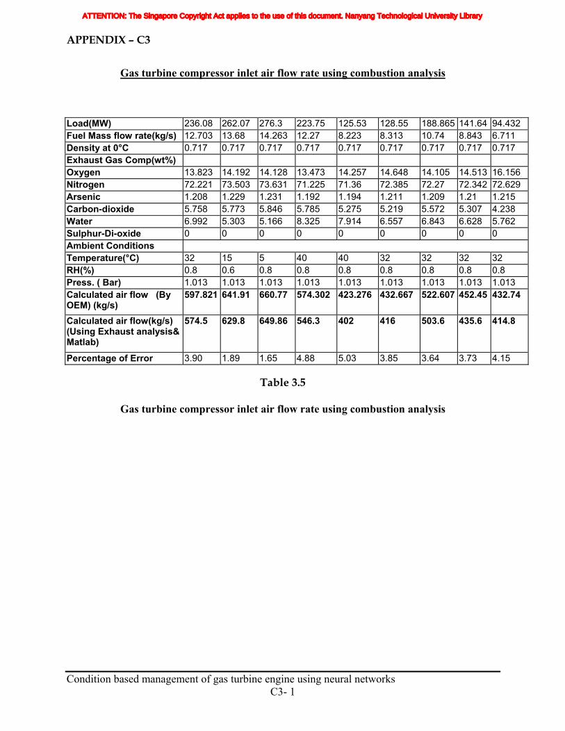
APPENDIX – C3
Gas turbine compressor inlet air flow rate using combustion analysis
Load(MW) 236.08 262.07 276.3 223.75 125.53 128.55 188.865 141.64 94.432 Fuel Mass flow rate(kg/s) 12.703 13.68 14.263 12.27 8.223 8.313 10.74 8.843 6.711 Density at 0°C 0.717 0.717 0.717 0.717 0.717 0.717 0.717 0.717 0.717 Exhaust Gas Comp(wt%) Oxygen 13.823 14.192 14.128 13.473 14.257 14.648 14.105 14.513 16.156 Nitrogen 72.221 73.503 73.631 71.225 71.36 72.385 72.27 72.342 72.629 Arsenic 1.208 1.229 1.231 1.192 1.194 1.211 1.209 1.21 1.215 Carbon-dioxide 5.758 5.773 5.846 5.785 5.275 5.219 5.572 5.307 4.238 Water 6.992 5.303 5.166 8.325 7.914 6.557 6.843 6.628 5.762 Sulphur-Di-oxide 0 0 0 0 0 0 0 0 0 Ambient Conditions Temperature(°C) 32 15 5 40 40 32 32 32 32 RH(%) 0.8 0.6 0.8 0.8 0.8 0.8 0.8 0.8 0.8 Press. ( Bar) 1.013 1.013 1.013 1.013 1.013 1.013 1.013 1.013 1.013 Calculated air flow (By OEM) (kg/s)
597.821 641.91 660.77 574.302 423.276 432.667 522.607 452.45 432.74
Calculated air flow(kg/s) (Using Exhaust analysis& Matlab)
574.5 629.8 649.86 546.3 402 416 503.6 435.6 414.8
Percentage of Error 3.90 1.89 1.65 4.88 5.03 3.85 3.64 3.73 4.15
Table 3.5
Gas turbine compressor inlet air flow rate using combustion analysis
Condition based management of gas turbine engine using neural networks
C3- 1
ATTENTION: The Singapore Copyright Act applies to the use of this document. Nanyang Technological University Library
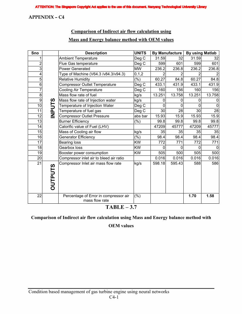
APPENDIX – C4
Comparison of Indirect air flow calculation using
Mass and Energy balance method with OEM values
Sno Description UNITS By Manufacture By using Matlab
1 Ambient Temperature Deg C 31.59 32 31.59 322 Flue Gas temperature Deg C 599 601 599 6013 Power Generated MW 236.2 236.8 236.2 236.84 Type of Machine (V64.3 /v84.3/v94.3) 0,1,2 2 2 2 25 Relative Humidity (%) 60.27 84.8 60.27 84.86 Compressor Outlet Temperature Deg C 433.1 431.9 433.1 431.97 Cooling Air Temperature Deg C 160 156 160 1568 Mass flow rate of fuel kg/s 13.251 13.758 13.251 13.7589 Mass flow rate of Injection water kg/s 0 0 0 0
10 Temperature of Injection Water Deg C 0 0 0 011 Temperature of fuel gas Deg C 30 28 30 2812 Compressor Outlet Pressure abs bar 15.93 15.9 15.93 15.913 Burner Efficiency (%) 99.8 99.8 99.8 99.814 Calorific value of Fuel (LHV) 47209 45777 47209 4577715 Mass of Cooling air flow kg/s 35 35 35 3516 Generator Efficiency (%) 98.4 98.4 98.4 98.417 Bearing loss KW 772 771 772 77118 Gearbox loss KW 0 0 0 019 Booster power consumption KW 505 500 505 50020
IN
PUTS
Compressor inlet air to bleed air ratio 0.016 0.016 0.016 0.01621
O
UTP
UTS
Compressor Inlet air mass flow rate kg/s 598.18 595.43 588 586
22 Percentage of Error in compressor air mass flow rate
(%) 1.70 1.58
TABLE – 3.7
Comparison of Indirect air flow calculation using Mass and Energy balance method with
OEM values
Condition based management of gas turbine engine using neural networks C4-1
ATTENTION: The Singapore Copyright Act applies to the use of this document. Nanyang Technological University Library
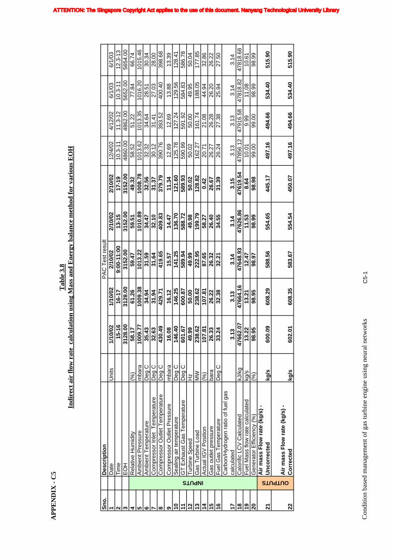
AP
PE
ND
IX -
C5
Tab
le 3
.8In
dire
ct a
ir fl
ow r
ate
cal
cula
tion
usi
ng M
ass
and
Ene
rgy
bala
nce
met
hod
for
vari
ous
EO
H
Sno
.D
escr
ipti
on
1
Dat
eU
nits
1/10
/02
1/10
/02
2/10
/02
2/10
/02
2/10
/02
12/4
/02
4/12
/02
6/1/
036/
1/03
2T
ime
15
-16
16-1
79:
00-1
1:00
13-1
517
-19
10.3
-11
11.3
-12
10.3
-11
12.3
-13
3E
OH
3128
.00
3128
.00
3152
.00
3152
.00
3152
.00
4860
.00
4862
.00
5652
.00
5654
.00
4R
elat
ive
Hum
idity
(%)
58.1
761
.26
59.4
759
.51
49.3
258
.52
51.2
277
.84
66.7
45
Am
bien
t Pre
ssur
em
bara
1009
.77
1009
.38
1013
.22
1010
.89
1008
.78
1013
.62
1013
.35
1016
.20
1015
.46
6A
mbi
ent T
empe
ratu
reD
eg C
35.4
334
.94
31.5
934
.47
32.5
632
.32
34.6
428
.51
30.3
47
Com
pres
sor
Inle
t T
empe
ratu
reD
eg C
32.6
331
.94
31.6
432
.10
31.3
730
.12
31.4
127
.03
28.0
08
Com
pres
sor
Out
let T
empe
ratu
reD
eg C
430.
4942
9.71
419.
6540
9.83
379.
7939
0.76
393.
5240
0.40
398.
689
Com
pres
sor
Out
let P
ress
ure
mba
ra16
.08
16.1
215
.57
14.4
711
.34
12.6
912
.69
13.8
813
.39
10S
ealin
g ai
r te
mpe
ratu
reD
eg C
146.
4014
6.25
141.
2513
6.70
121.
6012
5.78
127.
2412
9.56
128.
4111
GT
Exh
aust
Gas
Tem
pera
ture
Deg
C60
1.67
600.
8758
9.94
588.
7258
9.93
590.
9959
1.92
584.
8358
6.78
12T
urbi
ne S
peed
Hz
49.9
950
.00
49.9
949
.98
50.0
250
.02
50.0
049
.95
50.0
413
Gas
Tur
bine
Loa
dM
W23
8.62
238.
6222
2.95
199.
7912
8.82
162.
2716
1.74
188.
0517
7.85
14A
ctua
l IG
V P
ositi
on(%
)10
7.81
107.
8187
.65
58.2
70.
4220
.71
21.0
844
.94
32.8
615
Gas
out
let p
ress
ure
bara
26.3
326
.22
26.3
226
.40
26.6
726
.27
26.2
826
.20
26.2
216
Fue
l Gas
Tem
pera
ture
Deg
C33
.24
32.3
832
.21
34.5
531
.39
26.2
427
.38
25.9
427
.50
17C
arbo
n/H
ydro
gen
ratio
of f
uel g
as
calc
ulat
ed3.
133.
133.
143.
143.
153.
133.
133.
143.
1418
Cal
orifi
c LC
V C
alcu
late
dkJ
/kg
4766
2.07
4766
4.16
4764
8.93
4762
6.86
4761
9.54
4785
6.12
4791
6.58
4781
8.82
4781
8.68
19F
uel M
ass
flow
rat
e ca
lcul
ated
kg/s
13.2
213
.21
12.4
711
.53
8.64
10.0
19.
9911
.08
10.6
120
Gen
erat
or E
ffici
ency
(%
)(%
)98
.95
98.9
598
.97
98.9
998
.98
99.0
099
.00
98.9
998
.99
21A
ir m
ass
Flo
w r
ate
(kg
/s)
- U
nco
rrec
ted
kg/s
600.
0960
8.29
588.
5655
4.65
445.
1749
7.16
494.
6653
4.40
515.
90
22A
ir m
ass
Flo
w r
ate
(kg
/s)
- C
orr
ecte
dkg
/s60
2.01
608.
3558
3.67
554.
5445
0.07
497.
1649
4.66
534.
4051
5.90
OUTPUTSINPUTS
PA
C T
est r
esul
t
Con
ditio
n ba
sed
man
agem
ent o
f gas
turb
ine
engi
ne u
sing
neu
ral n
etw
orks
C5-
1
ATTENTION: The Singapore Copyright Act applies to the use of this document. Nanyang Technological University Library
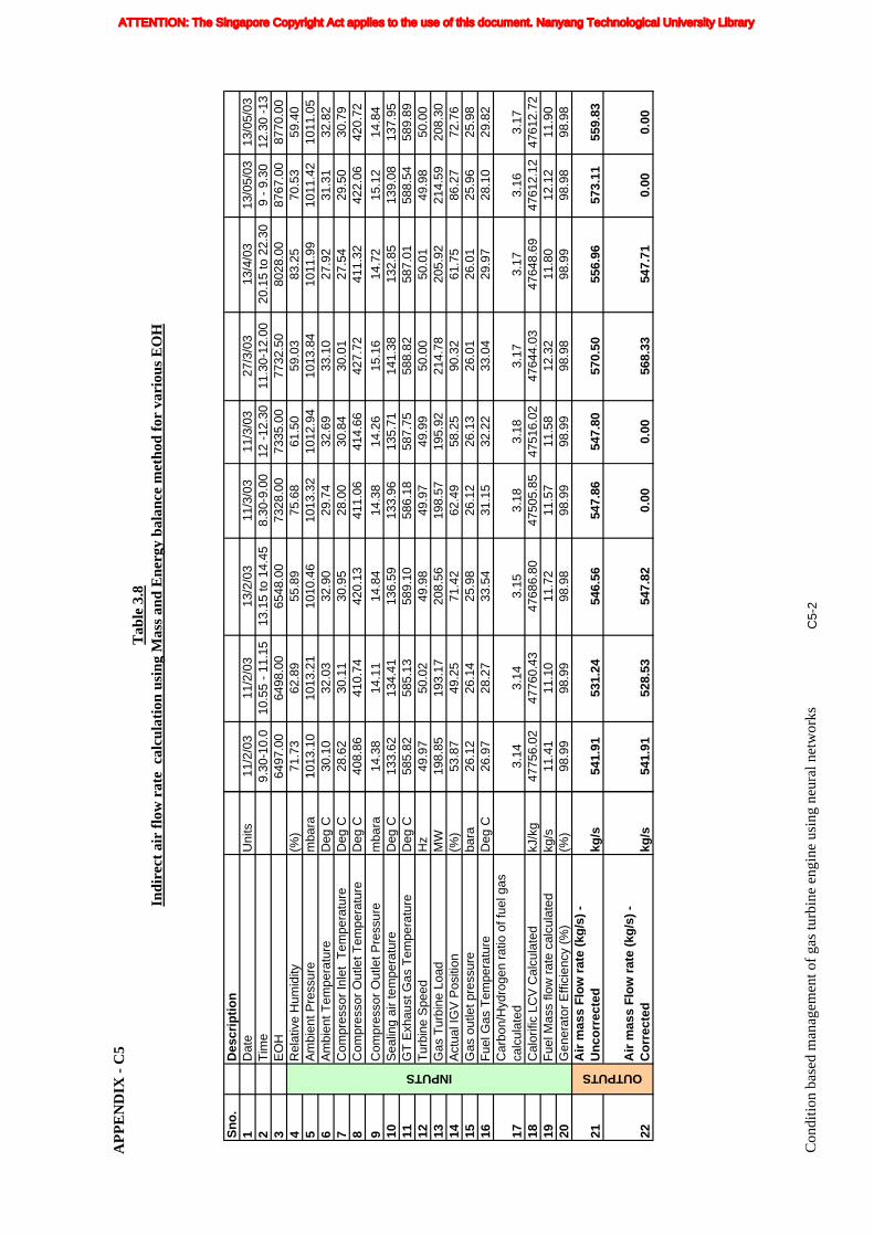
AP
PE
ND
IX -
C5
Tab
le 3
.8In
dire
ct a
ir fl
ow r
ate
cal
cula
tion
usi
ng M
ass
and
Ene
rgy
bala
nce
met
hod
for
vari
ous
EO
H
Sno
.D
escr
ipti
on
1
Dat
eU
nits
2T
ime
3E
OH
4R
elat
ive
Hum
idity
(%)
5A
mbi
ent P
ress
ure
mba
ra6
Am
bien
t Tem
pera
ture
Deg
C7
Com
pres
sor
Inle
t T
empe
ratu
reD
eg C
8C
ompr
esso
r O
utle
t Tem
pera
ture
Deg
C9
Com
pres
sor
Out
let P
ress
ure
mba
ra10
Sea
ling
air
tem
pera
ture
Deg
C11
GT
Exh
aust
Gas
Tem
pera
ture
Deg
C12
Tur
bine
Spe
edH
z13
Gas
Tur
bine
Loa
dM
W14
Act
ual I
GV
Pos
ition
(%)
15G
as o
utle
t pre
ssur
eba
ra16
Fue
l Gas
Tem
pera
ture
Deg
C
17C
arbo
n/H
ydro
gen
ratio
of f
uel g
as
calc
ulat
ed18
Cal
orifi
c LC
V C
alcu
late
dkJ
/kg
19F
uel M
ass
flow
rat
e ca
lcul
ated
kg/s
20G
ener
ator
Effi
cien
cy (
%)
(%)
21A
ir m
ass
Flo
w r
ate
(kg
/s)
- U
nco
rrec
ted
kg/s
22A
ir m
ass
Flo
w r
ate
(kg
/s)
- C
orr
ecte
dkg
/s
OUTPUTSINPUTS
11/2
/03
11/2
/03
13/2
/03
11/3
/03
11/3
/03
27/3
/03
13/4
/03
13/0
5/03
13/0
5/03
9.30
-10.
010
.55
- 11
.15
13.1
5 to
14.
458.
30-9
.00
12 -
12.3
011
.30-
12.0
020
.15
to 2
2.30
9 -
9.30
12.3
0 -1
364
97.0
064
98.0
065
48.0
073
28.0
073
35.0
077
32.5
080
28.0
087
67.0
087
70.0
071
.73
62.8
955
.89
75.6
861
.50
59.0
383
.25
70.5
359
.40
1013
.10
1013
.21
1010
.46
1013
.32
1012
.94
1013
.84
1011
.99
1011
.42
1011
.05
30.1
032
.03
32.9
029
.74
32.6
933
.10
27.9
231
.31
32.8
228
.62
30.1
130
.95
28.0
030
.84
30.0
127
.54
29.5
030
.79
408.
8641
0.74
420.
1341
1.06
414.
6642
7.72
411.
3242
2.06
420.
7214
.38
14.1
114
.84
14.3
814
.26
15.1
614
.72
15.1
214
.84
133.
6213
4.41
136.
5913
3.96
135.
7114
1.38
132.
8513
9.08
137.
9558
5.82
585.
1358
9.10
586.
1858
7.75
588.
8258
7.01
588.
5458
9.89
49.9
750
.02
49.9
849
.97
49.9
950
.00
50.0
149
.98
50.0
019
8.85
193.
1720
8.56
198.
5719
5.92
214.
7820
5.92
214.
5920
8.30
53.8
749
.25
71.4
262
.49
58.2
590
.32
61.7
586
.27
72.7
626
.12
26.1
425
.98
26.1
226
.13
26.0
126
.01
25.9
625
.98
26.9
728
.27
33.5
431
.15
32.2
233
.04
29.9
728
.10
29.8
2
3.14
3.14
3.15
3.18
3.18
3.17
3.17
3.16
3.17
4775
6.02
4776
0.43
4768
6.80
4750
5.85
4751
6.02
4764
4.03
4764
8.69
4761
2.12
4761
2.72
11.4
111
.10
11.7
211
.57
11.5
812
.32
11.8
012
.12
11.9
098
.99
98.9
998
.98
98.9
998
.99
98.9
898
.99
98.9
898
.98
541.
9153
1.24
546.
5654
7.86
547.
8057
0.50
556.
9657
3.11
559.
83
541.
9152
8.53
547.
820.
000.
0056
8.33
547.
710.
000.
00
Con
ditio
n ba
sed
man
agem
ent o
f gas
turb
ine
engi
ne u
sing
neu
ral n
etw
orks
C5-
2
ATTENTION: The Singapore Copyright Act applies to the use of this document. Nanyang Technological University Library
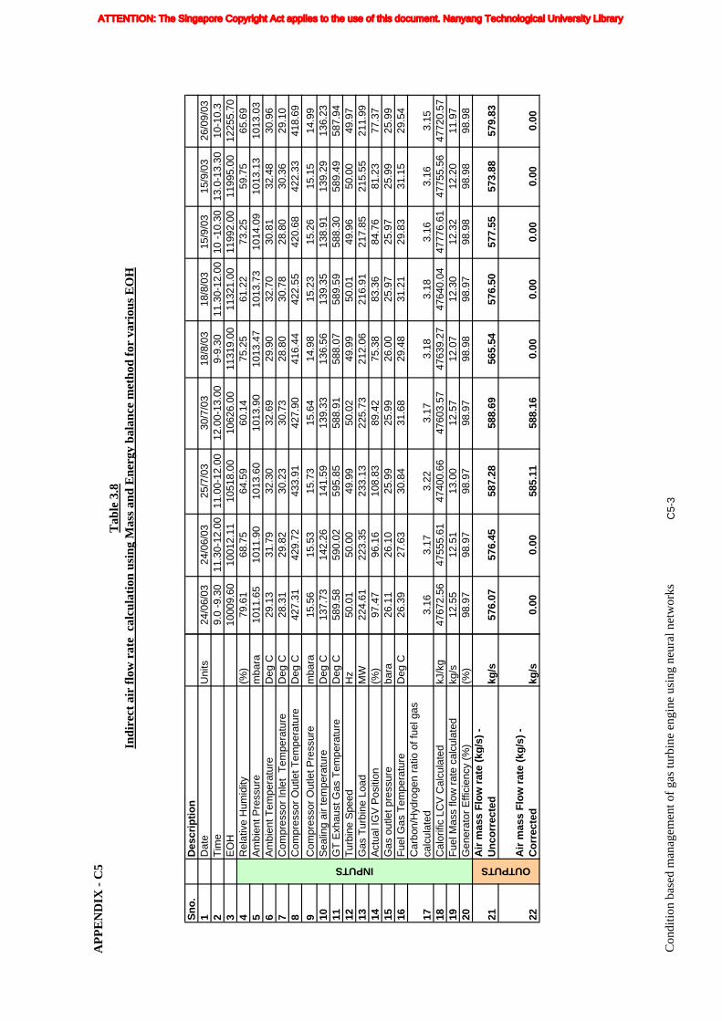
AP
PE
ND
IX -
C5
Tab
le 3
.8In
dire
ct a
ir fl
ow r
ate
cal
cula
tion
usi
ng M
ass
and
Ene
rgy
bala
nce
met
hod
for
vari
ous
EO
H
Sno
.D
escr
ipti
on
1
Dat
eU
nits
2T
ime
3E
OH
4R
elat
ive
Hum
idity
(%)
5A
mbi
ent P
ress
ure
mba
ra6
Am
bien
t Tem
pera
ture
Deg
C7
Com
pres
sor
Inle
t T
empe
ratu
reD
eg C
8C
ompr
esso
r O
utle
t Tem
pera
ture
Deg
C9
Com
pres
sor
Out
let P
ress
ure
mba
ra10
Sea
ling
air
tem
pera
ture
Deg
C11
GT
Exh
aust
Gas
Tem
pera
ture
Deg
C12
Tur
bine
Spe
edH
z13
Gas
Tur
bine
Loa
dM
W14
Act
ual I
GV
Pos
ition
(%)
15G
as o
utle
t pre
ssur
eba
ra16
Fue
l Gas
Tem
pera
ture
Deg
C
17C
arbo
n/H
ydro
gen
ratio
of f
uel g
as
calc
ulat
ed18
Cal
orifi
c LC
V C
alcu
late
dkJ
/kg
19F
uel M
ass
flow
rat
e ca
lcul
ated
kg/s
20G
ener
ator
Effi
cien
cy (
%)
(%)
21A
ir m
ass
Flo
w r
ate
(kg
/s)
- U
nco
rrec
ted
kg/s
22A
ir m
ass
Flo
w r
ate
(kg
/s)
- C
orr
ecte
dkg
/s
OUTPUTSINPUTS
24/0
6/03
24/0
6/03
25/7
/03
30/7
/03
18/8
/03
18/8
/03
15/9
/03
15/9
/03
26/0
9/03
9.0
-9.3
011
.30-
12.0
011
.00-
12.0
012
.00-
13.0
09-
9.30
11.3
0-12
.00
10 -
10.3
013
.0-1
3.30
10-1
0.3
1000
9.60
1001
2.11
1051
8.00
1062
6.00
1131
9.00
1132
1.00
1199
2.00
1199
5.00
1225
5.70
79.6
168
.75
64.5
960
.14
75.2
561
.22
73.2
559
.75
65.6
910
11.6
510
11.9
010
13.6
010
13.9
010
13.4
710
13.7
310
14.0
910
13.1
310
13.0
329
.13
31.7
932
.30
32.6
929
.90
32.7
030
.81
32.4
830
.96
28.3
129
.82
30.2
330
.73
28.8
030
.78
28.8
030
.36
29.1
042
7.31
429.
7243
3.91
427.
9041
6.44
422.
5542
0.68
422.
3341
8.69
15.5
615
.53
15.7
315
.64
14.9
815
.23
15.2
615
.15
14.9
913
7.73
142.
2614
1.59
139.
3313
6.56
139.
3513
8.91
139.
2913
6.23
589.
5859
0.02
595.
8558
8.91
588.
0758
9.59
588.
3058
9.49
587.
9450
.01
50.0
049
.99
50.0
249
.99
50.0
149
.96
50.0
049
.97
224.
6122
3.35
233.
1322
5.73
212.
0621
6.91
217.
8521
5.55
211.
9997
.47
96.1
610
8.83
89.4
275
.38
83.3
684
.76
81.2
377
.37
26.1
126
.10
25.9
925
.99
26.0
025
.97
25.9
725
.99
25.9
926
.39
27.6
330
.84
31.6
829
.48
31.2
129
.83
31.1
529
.54
3.16
3.17
3.22
3.17
3.18
3.18
3.16
3.16
3.15
4767
2.56
4755
5.61
4740
0.66
4760
3.57
4763
9.27
4764
0.04
4777
6.61
4775
5.56
4772
0.57
12.5
512
.51
13.0
012
.57
12.0
712
.30
12.3
212
.20
11.9
798
.97
98.9
798
.97
98.9
798
.98
98.9
798
.98
98.9
898
.98
576.
0757
6.45
587.
2858
8.69
565.
5457
6.50
577.
5557
3.88
579.
83
0.00
0.00
585.
1158
8.16
0.00
0.00
0.00
0.00
0.00
Con
ditio
n ba
sed
man
agem
ent o
f gas
turb
ine
engi
ne u
sing
neu
ral n
etw
orks
C5-
3
ATTENTION: The Singapore Copyright Act applies to the use of this document. Nanyang Technological University Library
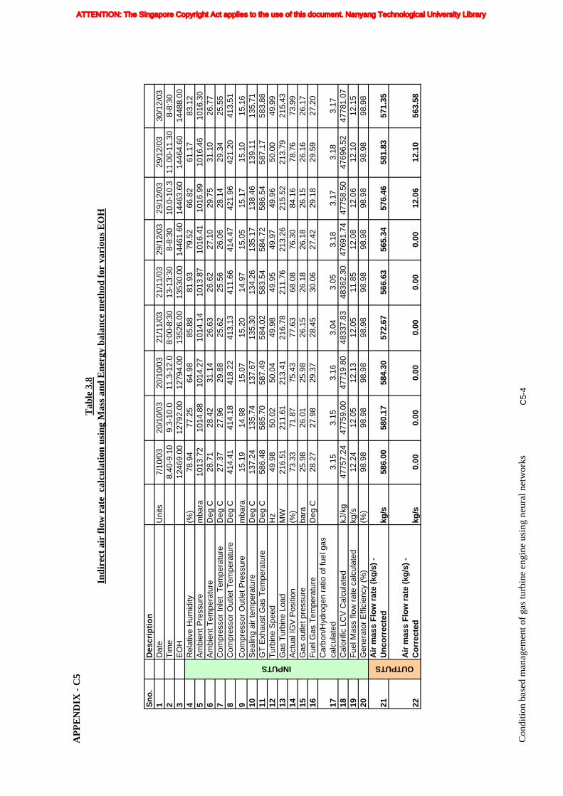
AP
PE
ND
IX -
C5
Tab
le 3
.8In
dire
ct a
ir fl
ow r
ate
cal
cula
tion
usi
ng M
ass
and
Ene
rgy
bala
nce
met
hod
for
vari
ous
EO
H
Sno
.D
escr
ipti
on
1
Dat
eU
nits
2T
ime
3E
OH
4R
elat
ive
Hum
idity
(%)
5A
mbi
ent P
ress
ure
mba
ra6
Am
bien
t Tem
pera
ture
Deg
C7
Com
pres
sor
Inle
t T
empe
ratu
reD
eg C
8C
ompr
esso
r O
utle
t Tem
pera
ture
Deg
C9
Com
pres
sor
Out
let P
ress
ure
mba
ra10
Sea
ling
air
tem
pera
ture
Deg
C11
GT
Exh
aust
Gas
Tem
pera
ture
Deg
C12
Tur
bine
Spe
edH
z13
Gas
Tur
bine
Loa
dM
W14
Act
ual I
GV
Pos
ition
(%)
15G
as o
utle
t pre
ssur
eba
ra16
Fue
l Gas
Tem
pera
ture
Deg
C
17C
arbo
n/H
ydro
gen
ratio
of f
uel g
as
calc
ulat
ed18
Cal
orifi
c LC
V C
alcu
late
dkJ
/kg
19F
uel M
ass
flow
rat
e ca
lcul
ated
kg/s
20G
ener
ator
Effi
cien
cy (
%)
(%)
21A
ir m
ass
Flo
w r
ate
(kg
/s)
- U
nco
rrec
ted
kg/s
22A
ir m
ass
Flo
w r
ate
(kg
/s)
- C
orr
ecte
dkg
/s
OUTPUTSINPUTS
7/10
/03
20/1
0/03
20/1
0/03
21/1
1/03
21/1
1/03
29/1
2/03
29/1
2/03
29/1
2/03
30/1
2/03
8.40
-9.1
09.
3-10
.011
.3-1
2.0
8:00
-8:3
013
-13:
308-
8:30
10.0
-10.
311
.00-
11.3
08-
8:30
1246
9.00
1279
2.00
1279
4.00
1352
6.00
1353
0.00
1446
1.60
1446
3.60
1446
4.60
1448
8.00
78.9
477
.25
64.9
885
.88
81.9
379
.52
66.8
261
.17
83.1
210
13.7
210
14.8
810
14.2
710
14.1
410
13.8
710
16.4
110
16.9
910
16.4
610
16.3
028
.71
28.4
231
.14
26.6
326
.62
27.1
029
.75
31.1
026
.77
27.3
727
.96
29.8
825
.62
25.5
626
.06
28.1
429
.34
25.5
541
4.41
414.
1841
8.22
413.
1341
1.66
414.
4742
1.96
421.
2041
3.51
15.1
914
.98
15.0
715
.20
14.9
715
.05
15.1
715
.10
15.1
613
7.24
135.
7413
7.67
135.
3013
4.26
135.
1713
8.46
139.
1113
5.71
586.
4858
5.70
587.
4958
4.02
583.
5458
4.72
586.
5458
7.17
583.
8849
.98
50.0
250
.04
49.9
849
.95
49.9
749
.96
50.0
049
.99
216.
5121
1.61
213.
4121
6.78
211.
7621
3.26
215.
5221
3.79
215.
4373
.33
71.8
775
.43
77.6
368
.08
76.3
084
.16
78.7
673
.99
25.9
826
.01
25.9
826
.15
26.1
826
.18
26.1
526
.16
26.1
728
.27
27.9
829
.37
28.4
530
.06
27.4
229
.18
29.5
927
.20
3.15
3.15
3.16
3.04
3.05
3.18
3.17
3.18
3.17
4775
7.24
4775
9.00
4771
9.80
4833
7.83
4836
2.30
4769
1.74
4775
8.50
4769
6.52
4778
1.07
12.2
412
.05
12.1
312
.05
11.8
512
.08
12.0
612
.10
12.1
598
.98
98.9
898
.98
98.9
898
.98
98.9
898
.98
98.9
898
.98
586.
0058
0.17
584.
3057
2.67
566.
6356
5.34
576.
4658
1.83
571.
35
0.00
0.00
0.00
0.00
0.00
0.00
12.0
612
.10
563.
58
Con
ditio
n ba
sed
man
agem
ent o
f gas
turb
ine
engi
ne u
sing
neu
ral n
etw
orks
C5-
4
ATTENTION: The Singapore Copyright Act applies to the use of this document. Nanyang Technological University Library
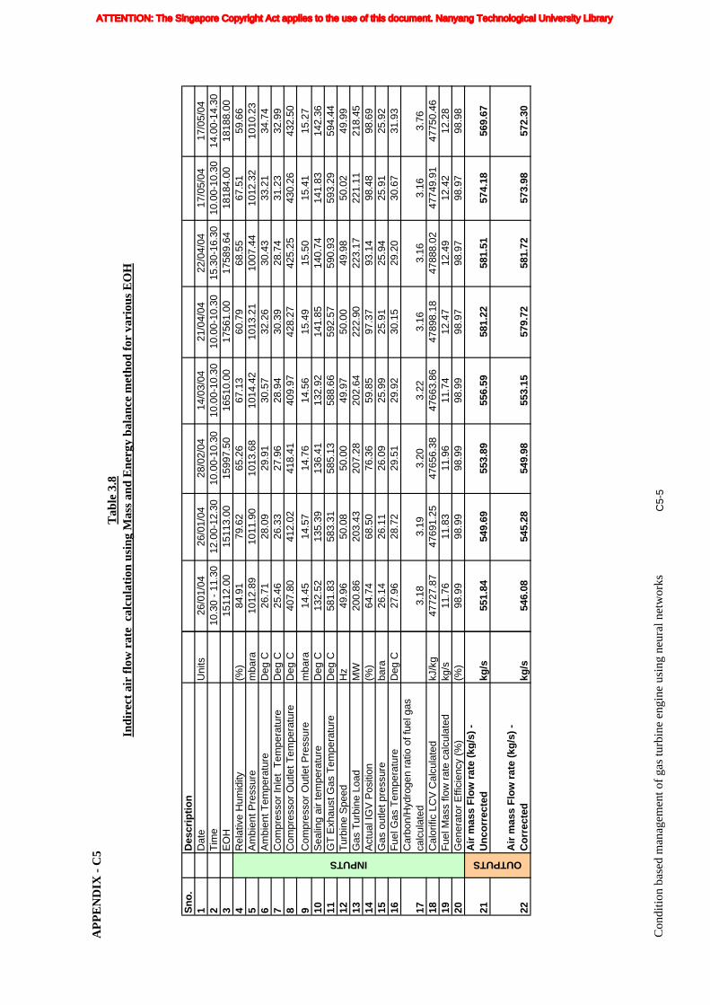
AP
PE
ND
IX -
C5
Tab
le 3
.8In
dire
ct a
ir fl
ow r
ate
cal
cula
tion
usi
ng M
ass
and
Ene
rgy
bala
nce
met
hod
for
vari
ous
EO
H
Sno
.D
escr
ipti
on
1
Dat
eU
nits
2T
ime
3E
OH
4R
elat
ive
Hum
idity
(%)
5A
mbi
ent P
ress
ure
mba
ra6
Am
bien
t Tem
pera
ture
Deg
C7
Com
pres
sor
Inle
t T
empe
ratu
reD
eg C
8C
ompr
esso
r O
utle
t Tem
pera
ture
Deg
C9
Com
pres
sor
Out
let P
ress
ure
mba
ra10
Sea
ling
air
tem
pera
ture
Deg
C11
GT
Exh
aust
Gas
Tem
pera
ture
Deg
C12
Tur
bine
Spe
edH
z13
Gas
Tur
bine
Loa
dM
W14
Act
ual I
GV
Pos
ition
(%)
15G
as o
utle
t pre
ssur
eba
ra16
Fue
l Gas
Tem
pera
ture
Deg
C
17C
arbo
n/H
ydro
gen
ratio
of f
uel g
as
calc
ulat
ed18
Cal
orifi
c LC
V C
alcu
late
dkJ
/kg
19F
uel M
ass
flow
rat
e ca
lcul
ated
kg/s
20G
ener
ator
Effi
cien
cy (
%)
(%)
21A
ir m
ass
Flo
w r
ate
(kg
/s)
- U
nco
rrec
ted
kg/s
22A
ir m
ass
Flo
w r
ate
(kg
/s)
- C
orr
ecte
dkg
/s
OUTPUTSINPUTS
26/0
1/04
26/0
1/04
28/0
2/04
14/0
3/04
21/0
4/04
22/0
4/04
17/0
5/04
17/0
5/04
10.3
0 -
11.3
012
.00-
12.3
010
.00-
10.3
010
.00-
10.3
010
.00-
10.3
015
.30-
16.3
010
.00-
10.3
014
.00-
14.3
015
112.
0015
113.
0015
997.
5016
510.
0017
561.
0017
589.
6418
184.
0018
188.
0084
.91
79.6
265
.26
67.1
360
.79
68.5
567
.51
59.6
610
12.8
910
11.9
010
13.6
810
14.4
210
13.2
110
07.4
410
12.3
210
10.2
326
.71
28.0
929
.91
30.5
732
.26
30.4
333
.21
34.7
425
.46
26.3
327
.96
28.9
430
.39
28.7
431
.23
32.9
940
7.80
412.
0241
8.41
409.
9742
8.27
425.
2543
0.26
432.
5014
.45
14.5
714
.76
14.5
615
.49
15.5
015
.41
15.2
713
2.52
135.
3913
6.41
132.
9214
1.85
140.
7414
1.83
142.
3658
1.83
583.
3158
5.13
588.
6659
2.57
590.
9359
3.29
594.
4449
.96
50.0
850
.00
49.9
750
.00
49.9
850
.02
49.9
920
0.86
203.
4320
7.28
202.
6422
2.90
223.
1722
1.11
218.
4564
.74
68.5
076
.36
59.8
597
.37
93.1
498
.48
98.6
926
.14
26.1
126
.09
25.9
925
.91
25.9
425
.91
25.9
227
.96
28.7
229
.51
29.9
230
.15
29.2
030
.67
31.9
3
3.18
3.19
3.20
3.22
3.16
3.16
3.16
3.76
4772
7.87
4769
1.25
4765
6.38
4766
3.86
4789
8.18
4788
8.02
4774
9.91
4775
0.46
11.7
611
.83
11.9
611
.74
12.4
712
.49
12.4
212
.28
98.9
998
.99
98.9
998
.99
98.9
798
.97
98.9
798
.98
551.
8454
9.69
553.
8955
6.59
581.
2258
1.51
574.
1856
9.67
546.
0854
5.28
549.
9855
3.15
579.
7258
1.72
573.
9857
2.30
Con
ditio
n ba
sed
man
agem
ent o
f gas
turb
ine
engi
ne u
sing
neu
ral n
etw
orks
C5-
5
ATTENTION: The Singapore Copyright Act applies to the use of this document. Nanyang Technological University Library
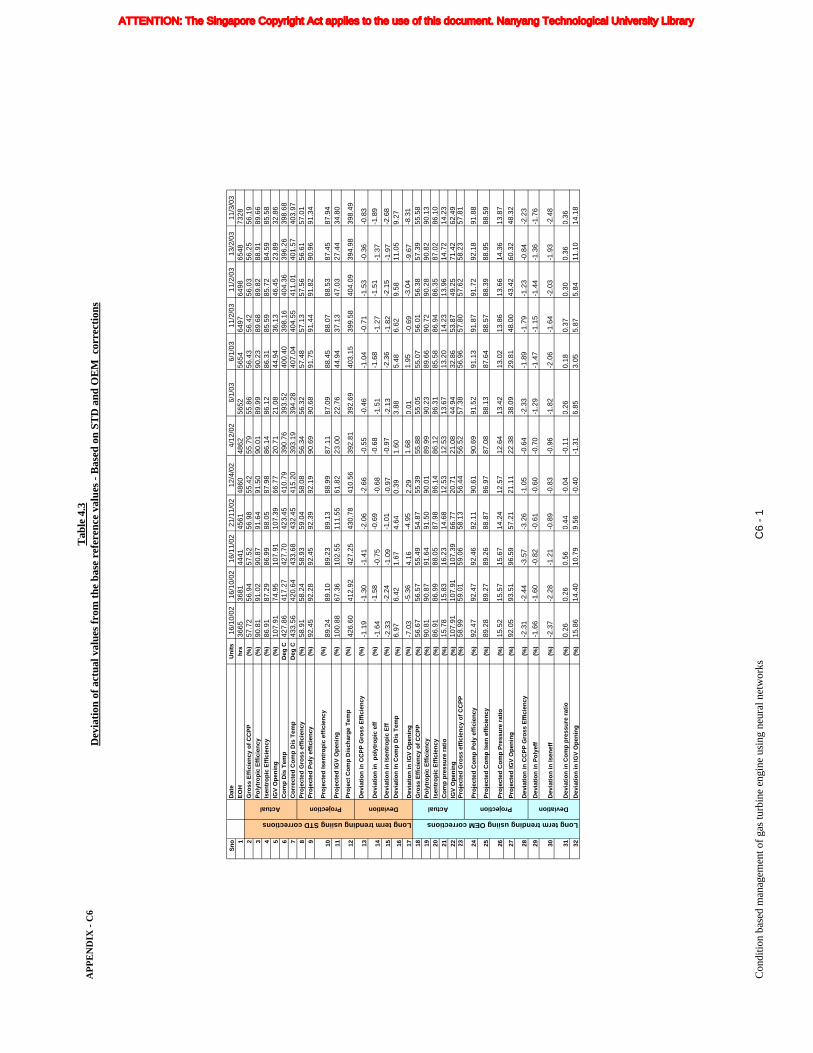
AP
PE
ND
IX -
C6
Tab
le 4
.3D
evia
tion
of a
ctua
l val
ues
from
the
base
ref
eren
ce v
alue
s - B
ased
on
STD
and
OE
M c
orre
ctio
ns
Sno
Dat
eU
nit
s16
/10/
0216
/10/
0216
/11/
0221
/11/
0212
/4/0
24/
12/0
26/
1/03
6/1/
0311
/2/0
311
/2/0
313
/2/0
311
/3/0
31
EO
Hh
rs36
6536
8144
4145
6148
6048
6256
5256
5464
9764
9865
4873
282
Gro
ss E
ffic
ien
cy o
f C
CP
P(%
)57
.72
56.9
457
.52
56.9
855
.42
55.7
955
.86
56.4
356
.42
56.0
356
.25
56.1
93
Po
lytr
op
ic E
ffic
ien
cy(%
)90
.81
91.0
290
.87
91.6
491
.50
90.0
189
.99
90.2
389
.68
89.8
288
.91
89.6
64
Isen
tro
pic
Eff
icie
ncy
(%)
86.9
187
.29
86.9
988
.05
87.9
886
.14
86.1
286
.31
85.5
985
.72
84.5
985
.58
5IG
V O
pen
ing
(%)
107.
9174
.95
107.
9110
7.39
66.7
720
.71
21.0
844
.94
36.1
346
.45
23.8
932
.86
6C
om
p D
is T
emp
Deg
C42
7.86
417.
2742
7.70
423.
4541
0.79
390.
7639
3.52
400.
4039
8.16
404.
3639
6.26
398.
687
Co
rrec
ted
Co
mp
Dis
Tem
pD
eg C
433.
5642
0.64
433.
6843
2.45
415.
2039
3.19
394.
2840
7.04
404.
5541
1.01
401.
5740
3.97
8P
roje
cted
Gro
ss e
ffic
ien
cy(%
)58
.91
58.2
458
.93
59.0
458
.08
56.3
456
.32
57.4
857
.13
57.5
656
.61
57.0
19
Pro
ject
ed P
oly
eff
icie
ncy
(%)
92.4
592
.28
92.4
592
.39
92.1
990
.69
90.6
891
.75
91.4
491
.82
90.9
691
.34
10P
roje
cted
Isen
tro
pic
eff
icie
ncy
(%)
89.2
489
.10
89.2
389
.13
88.9
987
.11
87.0
988
.45
88.0
788
.53
87.4
587
.94
11P
roje
cted
IGV
Op
enin
g(%
)10
0.88
67.3
610
2.55
111.
5561
.82
23.0
022
.76
44.9
437
.13
47.0
327
.44
34.8
0
12P
roje
ct C
om
p D
isch
arg
e T
emp
(%)
426.
6041
2.92
427.
2543
0.78
410.
5639
2.81
392.
6940
3.15
399.
5840
4.09
394.
9839
8.49
13D
evia
tio
n in
CC
PP
Gro
ss E
ffic
ien
cy(%
)-1
.19
-1.3
0-1
.41
-2.0
6-2
.66
-0.5
5-0
.46
-1.0
4-0
.71
-1.5
3-0
.36
-0.8
3
14D
evia
tio
n in
po
lytr
op
ic e
ff(%
)-1
.64
-1.5
8-0
.75
-0.6
9-0
.68
-0.6
8-1
.51
-1.6
8-1
.27
-1.5
1-1
.37
-1.8
9
15D
evia
tio
n in
Isen
tro
pic
Eff
(%)
-2.3
3-2
.24
-1.0
9-1
.01
-0.9
7-0
.97
-2.1
3-2
.36
-1.8
2-2
.15
-1.9
7-2
.68
16D
evia
tio
n In
Co
mp
Dis
Tem
p(%
)6.
976.
421.
674.
640.
391.
603.
885.
486.
629.
5811
.05
9.27
17D
evia
tio
n in
IGV
Op
enin
g(%
)-7
.03
-5.3
64.
16-4
.95
2.29
1.68
0.01
1.95
-0.6
9-3
.04
-9.6
7-8
.31
18G
ross
Eff
icie
ncy
of
CC
PP
(%)
56.6
756
.57
55.4
954
.87
55.3
955
.88
55.0
555
.07
56.0
156
.38
57.3
955
.58
19P
oly
tro
pic
Eff
icie
ncy
(%)
90.8
190
.87
91.6
491
.50
90.0
189
.99
90.2
389
.66
90.7
290
.28
90.8
290
.13
20Is
entr
op
ic E
ffic
ien
cy(%
)86
.91
86.9
988
.05
87.9
886
.14
86.1
286
.31
85.5
886
.94
86.3
587
.02
86.1
021
Co
mp
pre
ssu
re r
atio
(%)
15.7
815
.83
16.2
314
.68
12.5
312
.53
13.6
713
.20
14.2
313
.96
14.7
214
.23
22IG
V O
pen
ing
(%)
107.
9110
7.91
107.
3966
.77
20.7
121
.08
44.9
432
.86
53.8
749
.25
71.4
262
.49
23P
roje
cted
Gro
ss e
ffic
ien
cy o
f C
CP
P(%
)58
.99
59.0
159
.06
58.1
356
.44
56.5
257
.38
56.9
657
.80
57.6
258
.23
57.8
1
24P
roje
cted
Co
mp
Po
ly e
ffic
ien
cy(%
)92
.47
92.4
792
.46
92.1
190
.61
90.6
991
.52
91.1
391
.87
91.7
292
.18
91.8
8
25P
roje
cted
Co
mp
Isen
eff
icie
ncy
(%)
89.2
889
.27
89.2
688
.87
86.9
787
.08
88.1
387
.64
88.5
788
.39
88.9
588
.59
26P
roje
cted
Co
mp
Pre
ssu
re r
atio
(%)
15.5
215
.57
15.6
714
.24
12.5
712
.64
13.4
213
.02
13.8
613
.66
14.3
613
.87
27P
roje
cted
IGV
Op
enin
g(%
)92
.05
93.5
196
.59
57.2
121
.11
22.3
838
.09
29.8
148
.00
43.4
260
.32
48.3
2
28D
evia
tio
n in
CC
PP
Gro
ss E
ffic
ien
cy(%
)-2
.31
-2.4
4-3
.57
-3.2
6-1
.05
-0.6
4-2
.33
-1.8
9-1
.79
-1.2
3-0
.84
-2.2
3
29D
evia
tio
n in
Po
lyef
f(%
)-1
.66
-1.6
0-0
.82
-0.6
1-0
.60
-0.7
0-1
.29
-1.4
7-1
.15
-1.4
4-1
.36
-1.7
6
30D
evia
tio
n in
Isen
eff
(%)
-2.3
7-2
.28
-1.2
1-0
.89
-0.8
3-0
.96
-1.8
2-2
.06
-1.6
4-2
.03
-1.9
3-2
.48
31D
evia
tio
n in
Co
mp
pre
ssu
re r
atio
(%)
0.26
0.26
0.56
0.44
-0.0
4-0
.11
0.26
0.18
0.37
0.30
0.36
0.36
32D
evia
tio
n in
IGV
Op
enin
g(%
)15
.86
14.4
010
.79
9.56
-0.4
0-1
.31
6.85
3.05
5.87
5.84
11.1
014
.18
Long term trending usiing STD corrections Long term trending usiing OEM corrections
Actual Projection DeviationActual Projection Deviation
Con
ditio
n ba
sed
man
agem
ent o
f gas
turb
ine
engi
ne u
sing
neu
ral n
etw
orks
C6
- 1
ATTENTION: The Singapore Copyright Act applies to the use of this document. Nanyang Technological University Library
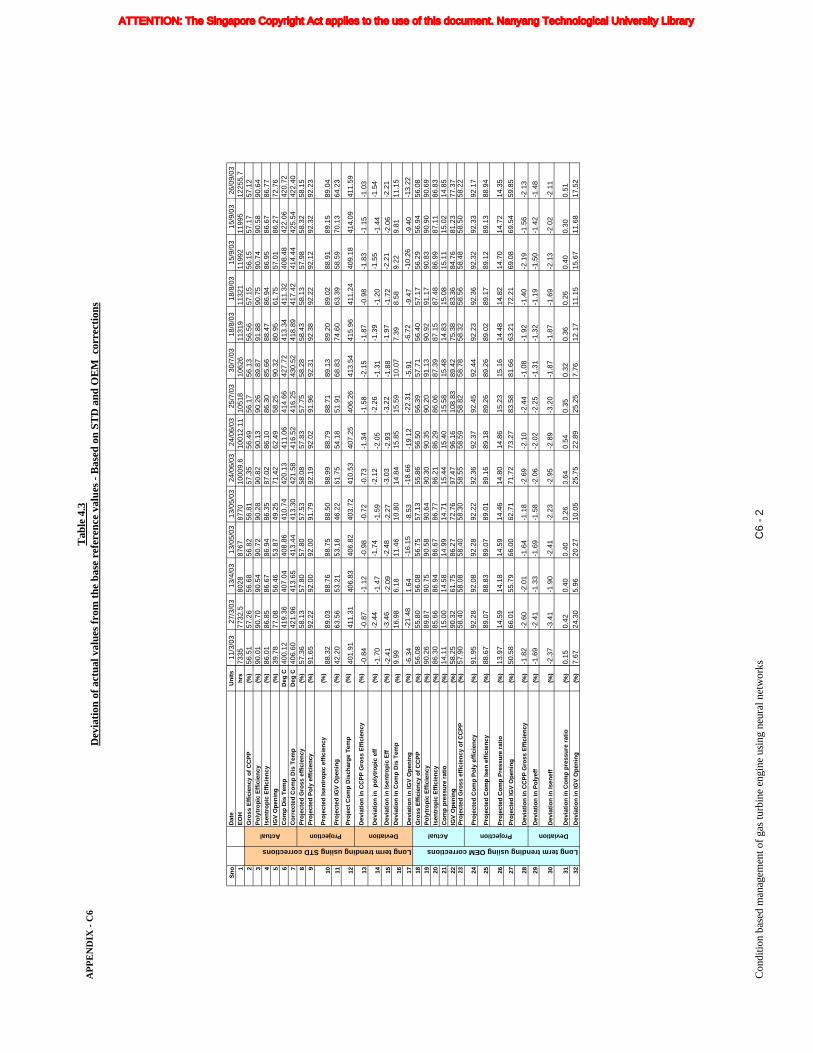
AP
PE
ND
IX -
C6
Tab
le 4
.3D
evia
tion
of a
ctua
l val
ues
from
the
base
ref
eren
ce v
alue
s - B
ased
on
STD
and
OE
M c
orre
ctio
ns
Sno
Dat
eU
nit
s
1E
OH
hrs
2G
ross
Eff
icie
ncy
of
CC
PP
(%)
3P
oly
tro
pic
Eff
icie
ncy
(%)
4Is
entr
op
ic E
ffic
ien
cy(%
)
5IG
V O
pen
ing
(%)
6C
om
p D
is T
emp
Deg
C
7C
orr
ecte
d C
om
p D
is T
emp
Deg
C
8P
roje
cted
Gro
ss e
ffic
ien
cy(%
)
9P
roje
cted
Po
ly e
ffic
ien
cy(%
)
10P
roje
cted
Isen
tro
pic
eff
icie
ncy
(%)
11P
roje
cted
IGV
Op
enin
g(%
)
12P
roje
ct C
om
p D
isch
arg
e T
emp
(%)
13D
evia
tio
n in
CC
PP
Gro
ss E
ffic
ien
cy(%
)
14D
evia
tio
n in
po
lytr
op
ic e
ff(%
)
15D
evia
tio
n in
Isen
tro
pic
Eff
(%)
16D
evia
tio
n In
Co
mp
Dis
Tem
p(%
)
17D
evia
tio
n in
IGV
Op
enin
g(%
)
18G
ross
Eff
icie
ncy
of
CC
PP
(%)
19P
oly
tro
pic
Eff
icie
ncy
(%)
20Is
entr
op
ic E
ffic
ien
cy(%
)21
Co
mp
pre
ssu
re r
atio
(%)
22IG
V O
pen
ing
(%)
23P
roje
cted
Gro
ss e
ffic
ien
cy o
f C
CP
P(%
)
24P
roje
cted
Co
mp
Po
ly e
ffic
ien
cy(%
)
25P
roje
cted
Co
mp
Isen
eff
icie
ncy
(%)
26P
roje
cted
Co
mp
Pre
ssu
re r
atio
(%)
27P
roje
cted
IGV
Op
enin
g(%
)
28D
evia
tio
n in
CC
PP
Gro
ss E
ffic
ien
cy(%
)
29D
evia
tio
n in
Po
lyef
f(%
)
30D
evia
tio
n in
Isen
eff
(%)
31D
evia
tio
n in
Co
mp
pre
ssu
re r
atio
(%)
32D
evia
tio
n in
IGV
Op
enin
g(%
)
Long term trending usiing STD corrections Long term trending usiing OEM corrections
Actual Projection DeviationActual Projection Deviation
11/3
/03
27/3
/03
13/4
/03
13/0
5/03
13/0
5/03
24/0
6/03
24/0
6/03
25/7
/03
30/7
/03
18/8
/03
18/8
/03
15/9
/03
15/9
/03
26/0
9/03
7335
7732
.580
2887
6787
7010
009.
610
012.
1110
518
1062
611
319
1132
111
992
1199
512
255.
756
.51
57.2
656
.68
56.8
256
.81
57.3
556
.49
56.1
756
.13
56.5
657
.15
56.1
557
.17
57.1
290
.01
90.7
090
.54
90.7
290
.28
90.8
290
.13
90.2
689
.87
91.8
890
.75
90.7
490
.58
90.6
486
.01
86.8
586
.67
86.9
486
.35
87.0
286
.10
86.3
085
.66
88.4
786
.94
86.9
586
.67
86.7
739
.78
77.0
856
.46
53.8
749
.25
71.4
262
.49
58.2
590
.32
80.9
561
.75
57.0
186
.27
72.7
640
0.12
419.
3640
7.04
408.
8641
0.74
420.
1341
1.06
414.
6642
7.72
413.
3441
1.32
408.
4842
2.06
420.
7240
6.60
421.
9641
3.65
413.
4441
3.30
421.
5841
6.52
416.
2543
0.52
418.
8941
7.42
414.
4442
5.54
422.
4057
.36
58.1
357
.80
57.8
057
.53
58.0
857
.83
57.7
558
.28
58.4
358
.13
57.9
858
.32
58.1
591
.65
92.2
292
.00
92.0
091
.79
92.1
992
.02
91.9
692
.31
92.3
892
.22
92.1
292
.32
92.2
3
88.3
289
.03
88.7
688
.75
88.5
088
.99
88.7
988
.71
89.1
389
.20
89.0
288
.91
89.1
589
.04
42.2
063
.56
53.2
153
.18
46.2
261
.75
54.1
851
.91
68.8
374
.60
63.3
958
.59
70.1
364
.23
401.
9141
1.31
406.
8340
6.82
403.
7241
0.53
407.
2540
6.26
413.
5441
5.96
411.
2440
9.18
414.
0941
1.59
-0.8
4-0
.87
-1.1
2-0
.98
-0.7
2-0
.73
-1.3
4-1
.58
-2.1
5-1
.87
-0.9
8-1
.83
-1.1
5-1
.03
-1.7
0-2
.44
-1.4
7-1
.74
-1.5
9-2
.12
-2.0
5-2
.26
-1.3
1-1
.39
-1.2
0-1
.55
-1.4
4-1
.54
-2.4
1-3
.46
-2.0
9-2
.48
-2.2
7-3
.03
-2.9
3-3
.22
-1.8
8-1
.97
-1.7
2-2
.21
-2.0
6-2
.21
9.99
16.9
86.
1811
.46
10.8
014
.84
15.8
515
.59
10.0
77.
398.
589.
229.
8111
.15
-6.3
4-2
1.48
1.64
-16.
15-8
.53
-18.
66-1
9.12
-22.
31-5
.91
-6.7
2-9
.47
-10.
26-9
.40
-13.
2256
.08
55.8
056
.08
56.7
557
.13
55.8
656
.50
56.3
957
.71
56.4
057
.17
56.2
956
.94
56.0
890
.26
89.8
790
.75
90.5
890
.64
90.3
090
.35
90.2
091
.13
90.9
291
.17
90.8
390
.90
90.6
986
.30
85.6
686
.94
86.6
786
.77
86.2
186
.29
86.0
687
.39
87.1
587
.48
86.9
987
.11
86.8
314
.11
15.0
014
.58
14.9
914
.71
15.4
415
.40
15.5
815
.48
14.8
315
.08
15.1
115
.02
14.8
558
.25
90.3
261
.75
86.2
772
.76
97.4
796
.16
108.
8389
.42
75.3
883
.36
84.7
681
.23
77.3
757
.90
58.4
058
.08
58.4
058
.30
58.5
558
.59
58.8
258
.78
58.3
258
.56
58.4
858
.50
58.2
2
91.9
592
.28
92.0
892
.28
92.2
292
.36
92.3
792
.45
92.4
492
.23
92.3
692
.32
92.3
392
.17
88.6
789
.07
88.8
389
.07
89.0
189
.16
89.1
889
.26
89.2
689
.02
89.1
789
.12
89.1
388
.94
13.9
714
.59
14.1
814
.59
14.4
614
.80
14.8
615
.23
15.1
614
.48
14.8
214
.70
14.7
214
.35
50.5
866
.01
55.7
966
.00
62.7
171
.72
73.2
783
.58
81.6
663
.21
72.2
169
.08
69.5
459
.85
-1.8
2-2
.60
-2.0
1-1
.64
-1.1
8-2
.69
-2.1
0-2
.44
-1.0
8-1
.92
-1.4
0-2
.19
-1.5
6-2
.13
-1.6
9-2
.41
-1.3
3-1
.69
-1.5
8-2
.06
-2.0
2-2
.25
-1.3
1-1
.32
-1.1
9-1
.50
-1.4
2-1
.48
-2.3
7-3
.41
-1.9
0-2
.41
-2.2
3-2
.95
-2.8
9-3
.20
-1.8
7-1
.87
-1.6
9-2
.13
-2.0
2-2
.11
0.15
0.42
0.40
0.40
0.26
0.64
0.54
0.35
0.32
0.36
0.26
0.40
0.30
0.51
7.67
24.3
05.
9620
.27
10.0
525
.75
22.8
925
.25
7.76
12.1
711
.15
15.6
711
.68
17.5
2
Con
ditio
n ba
sed
man
agem
ent o
f gas
turb
ine
engi
ne u
sing
neu
ral n
etw
orks
C6
- 2
ATTENTION: The Singapore Copyright Act applies to the use of this document. Nanyang Technological University Library
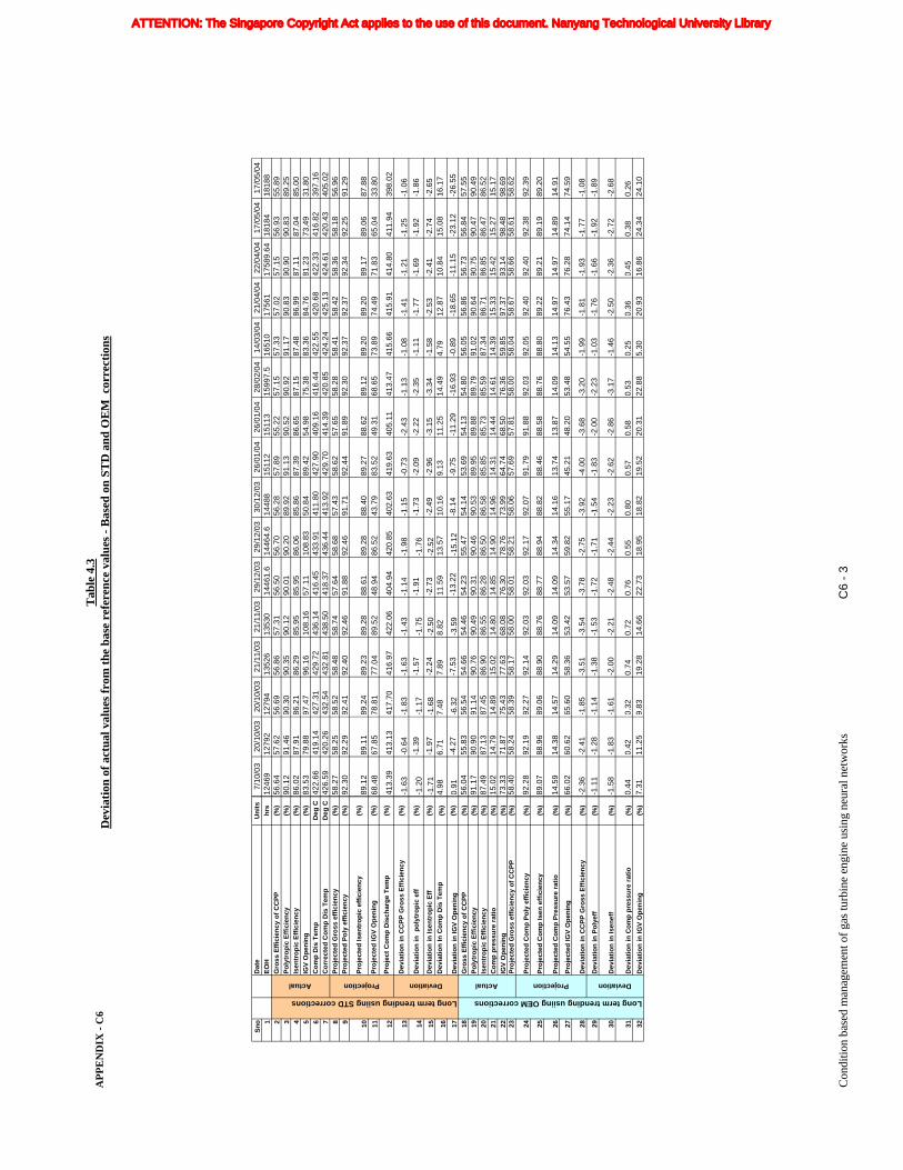
AP
PE
ND
IX -
C6
Tab
le 4
.3D
evia
tion
of a
ctua
l val
ues
from
the
base
ref
eren
ce v
alue
s - B
ased
on
STD
and
OE
M c
orre
ctio
ns
Sno
Dat
eU
nit
s
1E
OH
hrs
2G
ross
Eff
icie
ncy
of
CC
PP
(%)
3P
oly
tro
pic
Eff
icie
ncy
(%)
4Is
entr
op
ic E
ffic
ien
cy(%
)
5IG
V O
pen
ing
(%)
6C
om
p D
is T
emp
Deg
C
7C
orr
ecte
d C
om
p D
is T
emp
Deg
C
8P
roje
cted
Gro
ss e
ffic
ien
cy(%
)
9P
roje
cted
Po
ly e
ffic
ien
cy(%
)
10P
roje
cted
Isen
tro
pic
eff
icie
ncy
(%)
11P
roje
cted
IGV
Op
enin
g(%
)
12P
roje
ct C
om
p D
isch
arg
e T
emp
(%)
13D
evia
tio
n in
CC
PP
Gro
ss E
ffic
ien
cy(%
)
14D
evia
tio
n in
po
lytr
op
ic e
ff(%
)
15D
evia
tio
n in
Isen
tro
pic
Eff
(%)
16D
evia
tio
n In
Co
mp
Dis
Tem
p(%
)
17D
evia
tio
n in
IGV
Op
enin
g(%
)
18G
ross
Eff
icie
ncy
of
CC
PP
(%)
19P
oly
tro
pic
Eff
icie
ncy
(%)
20Is
entr
op
ic E
ffic
ien
cy(%
)21
Co
mp
pre
ssu
re r
atio
(%)
22IG
V O
pen
ing
(%)
23P
roje
cted
Gro
ss e
ffic
ien
cy o
f C
CP
P(%
)
24P
roje
cted
Co
mp
Po
ly e
ffic
ien
cy(%
)
25P
roje
cted
Co
mp
Isen
eff
icie
ncy
(%)
26P
roje
cted
Co
mp
Pre
ssu
re r
atio
(%)
27P
roje
cted
IGV
Op
enin
g(%
)
28D
evia
tio
n in
CC
PP
Gro
ss E
ffic
ien
cy(%
)
29D
evia
tio
n in
Po
lyef
f(%
)
30D
evia
tio
n in
Isen
eff
(%)
31D
evia
tio
n in
Co
mp
pre
ssu
re r
atio
(%)
32D
evia
tio
n in
IGV
Op
enin
g(%
)
Long term trending usiing STD corrections Long term trending usiing OEM corrections
Actual Projection DeviationActual Projection Deviation
7/10
/03
20/1
0/03
20/1
0/03
21/1
1/03
21/1
1/03
29/1
2/03
29/1
2/03
30/1
2/03
26/0
1/04
26/0
1/04
28/0
2/04
14/0
3/04
21/0
4/04
22/0
4/04
17/0
5/04
17/0
5/04
1246
912
792
1279
413
526
1353
014
461.
614
464.
614
488
1511
215
113
1599
7.5
1651
017
561
1758
9.64
1818
418
188
56.6
457
.62
56.6
956
.86
57.3
156
.50
56.7
056
.28
57.8
955
.22
57.1
557
.33
57.0
257
.15
56.9
355
.89
90.1
291
.46
90.3
090
.35
90.1
290
.01
90.2
089
.92
91.1
390
.52
90.9
291
.17
90.8
390
.90
90.8
389
.25
86.0
287
.91
86.2
186
.29
85.9
585
.95
86.0
685
.86
87.3
986
.65
87.1
587
.48
86.9
987
.11
87.0
485
.00
83.5
379
.88
97.4
796
.16
108.
1657
.11
108.
8350
.84
89.4
254
.98
75.3
883
.36
84.7
681
.23
73.4
931
.80
422.
6641
9.14
427.
3142
9.72
436.
1441
6.45
433.
9141
1.80
427.
9040
9.16
416.
4442
2.55
420.
6842
2.33
416.
8239
7.16
426.
5942
0.26
432.
5443
2.81
438.
5041
8.37
436.
4441
3.92
429.
7041
4.39
420.
8542
4.24
425.
1342
4.61
420.
4340
5.02
58.2
758
.25
58.5
258
.48
58.7
457
.64
58.6
857
.43
58.6
257
.65
58.2
858
.41
58.4
258
.36
58.1
856
.96
92.3
092
.29
92.4
192
.40
92.4
691
.88
92.4
691
.71
92.4
491
.89
92.3
092
.37
92.3
792
.34
92.2
591
.29
89.1
289
.11
89.2
489
.23
89.2
888
.61
89.2
888
.40
89.2
788
.62
89.1
289
.20
89.2
089
.17
89.0
687
.88
68.4
867
.85
78.8
177
.04
89.5
248
.94
86.5
243
.79
83.5
249
.31
68.6
573
.89
74.4
971
.83
65.0
433
.80
413.
3941
3.13
417.
7041
6.97
422.
0640
4.94
420.
8540
2.63
419.
6340
5.11
413.
4741
5.66
415.
9141
4.80
411.
9439
8.02
-1.6
3-0
.64
-1.8
3-1
.63
-1.4
3-1
.14
-1.9
8-1
.15
-0.7
3-2
.43
-1.1
3-1
.08
-1.4
1-1
.21
-1.2
5-1
.06
-1.2
0-1
.39
-1.1
7-1
.57
-1.7
5-1
.91
-1.7
6-1
.73
-2.0
9-2
.22
-2.3
5-1
.11
-1.7
7-1
.69
-1.9
2-1
.86
-1.7
1-1
.97
-1.6
8-2
.24
-2.5
0-2
.73
-2.5
2-2
.49
-2.9
6-3
.15
-3.3
4-1
.58
-2.5
3-2
.41
-2.7
4-2
.65
4.98
6.71
7.48
7.89
8.82
11.5
913
.57
10.1
69.
1311
.25
14.4
94.
7912
.87
10.8
415
.08
16.1
7
0.91
-4.2
7-6
.32
-7.5
3-3
.59
-13.
22-1
5.12
-8.1
4-9
.75
-11.
29-1
6.93
-0.8
9-1
8.65
-11.
15-2
3.12
-26.
5556
.04
55.8
356
.54
54.6
654
.46
54.2
355
.47
54.1
453
.69
54.1
354
.80
56.0
556
.86
56.7
356
.84
57.5
591
.17
90.9
091
.14
90.7
690
.49
90.3
190
.46
90.5
389
.95
89.8
889
.79
91.0
290
.64
90.7
590
.47
90.4
987
.49
87.1
387
.45
86.9
086
.55
86.2
886
.50
86.5
885
.85
85.7
385
.59
87.3
486
.71
86.8
586
.47
86.5
215
.02
14.7
914
.89
15.0
214
.80
14.8
514
.90
14.9
614
.31
14.4
414
.61
14.3
915
.33
15.4
215
.27
15.1
773
.33
71.8
775
.43
77.6
368
.08
76.3
078
.76
73.9
964
.74
68.5
076
.36
59.8
597
.37
93.1
498
.48
98.6
958
.40
58.2
458
.39
58.1
758
.00
58.0
158
.21
58.0
657
.69
57.8
158
.00
58.0
458
.67
58.6
658
.61
58.6
2
92.2
892
.19
92.2
792
.14
92.0
392
.03
92.1
792
.07
91.7
991
.88
92.0
392
.05
92.4
092
.40
92.3
892
.39
89.0
788
.96
89.0
688
.90
88.7
688
.77
88.9
488
.82
88.4
688
.58
88.7
688
.80
89.2
289
.21
89.1
989
.20
14.5
914
.38
14.5
714
.29
14.0
914
.09
14.3
414
.16
13.7
413
.87
14.0
914
.13
14.9
714
.97
14.8
914
.91
66.0
260
.62
65.6
058
.36
53.4
253
.57
59.8
255
.17
45.2
148
.20
53.4
854
.55
76.4
376
.28
74.1
474
.59
-2.3
6-2
.41
-1.8
5-3
.51
-3.5
4-3
.78
-2.7
5-3
.92
-4.0
0-3
.68
-3.2
0-1
.99
-1.8
1-1
.93
-1.7
7-1
.08
-1.1
1-1
.28
-1.1
4-1
.38
-1.5
3-1
.72
-1.7
1-1
.54
-1.8
3-2
.00
-2.2
3-1
.03
-1.7
6-1
.66
-1.9
2-1
.89
-1.5
8-1
.83
-1.6
1-2
.00
-2.2
1-2
.48
-2.4
4-2
.23
-2.6
2-2
.86
-3.1
7-1
.46
-2.5
0-2
.36
-2.7
2-2
.68
0.44
0.42
0.32
0.74
0.72
0.76
0.55
0.80
0.57
0.58
0.53
0.25
0.36
0.45
0.38
0.26
7.31
11.2
59.
8319
.28
14.6
622
.73
18.9
518
.82
19.5
220
.31
22.8
85.
3020
.93
16.8
624
.34
24.1
0
Con
ditio
n ba
sed
man
agem
ent o
f gas
turb
ine
engi
ne u
sing
neu
ral n
etw
orks
C6
- 3
ATTENTION: The Singapore Copyright Act applies to the use of this document. Nanyang Technological University Library

Appendix D
ATTENTION: The Singapore Copyright Act applies to the use of this document. Nanyang Technological University Library
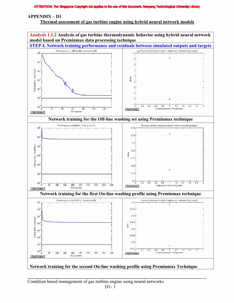
APPENDIX – D1 Thermal assessment of gas turbine engine using hybrid neural network models
Analysis 1.1.2 Analysis of gas turbine thermodynamic behavior using hybrid neural network model based on Preminmax data processing technique STEP-I. Network training performance and residuals between simulated outputs and targets
Network training for the Off-line washing set using Preminmax technique
Network training for the first On-line washing profile using Preminmax technique
Network training for the second On-line washing profile using Preminmax Technique
______________________________________________________________________________ Condition based management of gas turbine engine using neural networks D1- 1
ATTENTION: The Singapore Copyright Act applies to the use of this document. Nanyang Technological University Library
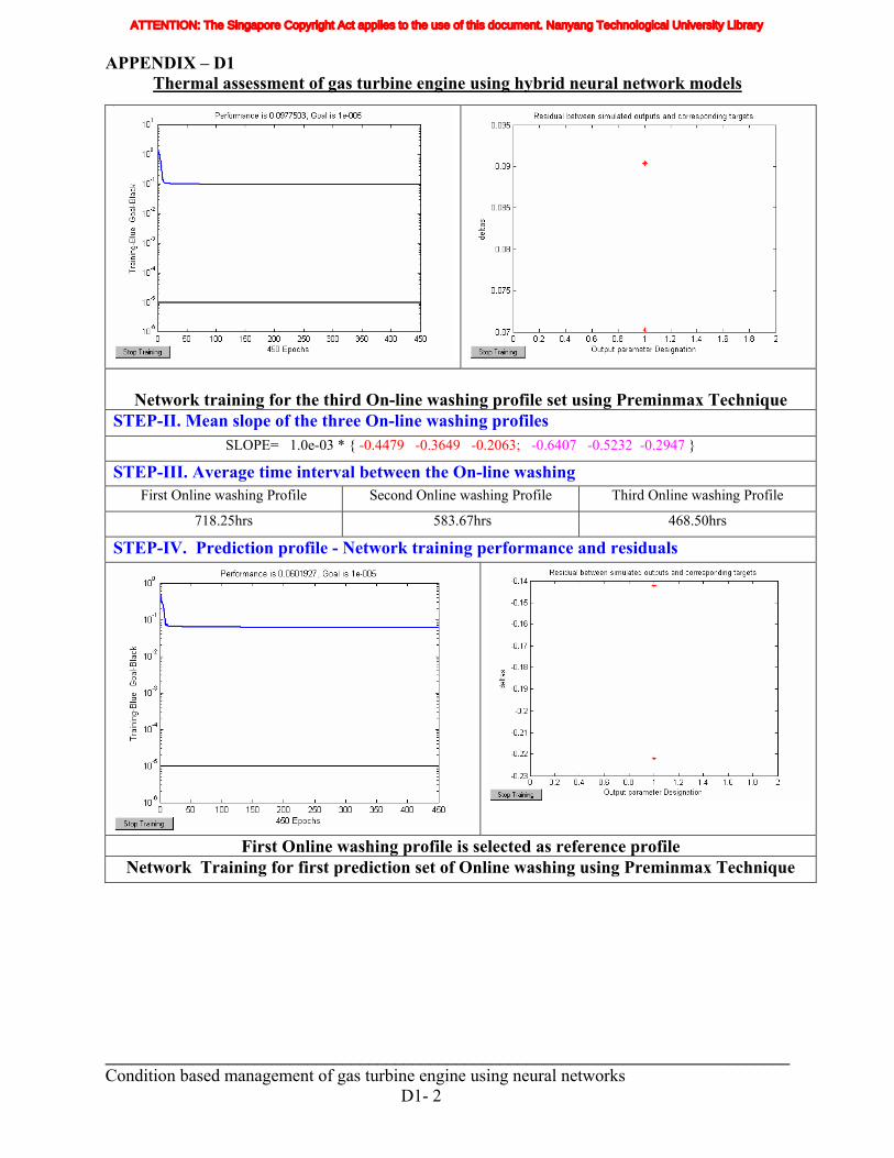
APPENDIX – D1 Thermal assessment of gas turbine engine using hybrid neural network models
Network training for the third On-line washing profile set using Preminmax Technique
STEP-II. Mean slope of the three On-line washing profiles SLOPE= 1.0e-03 * { -0.4479 -0.3649 -0.2063; -0.6407 -0.5232 -0.2947 }
STEP-III. Average time interval between the On-line washing First Online washing Profile Second Online washing Profile Third Online washing Profile
718.25hrs 583.67hrs 468.50hrs
STEP-IV. Prediction profile - Network training performance and residuals
First Online washing profile is selected as reference profile Network Training for first prediction set of Online washing using Preminmax Technique
______________________________________________________________________________ Condition based management of gas turbine engine using neural networks D1- 2
ATTENTION: The Singapore Copyright Act applies to the use of this document. Nanyang Technological University Library
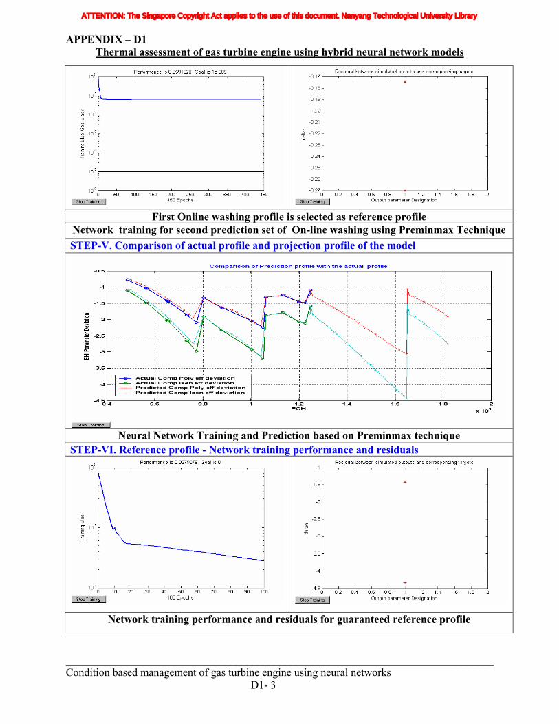
APPENDIX – D1 Thermal assessment of gas turbine engine using hybrid neural network models
First Online washing profile is selected as reference profile
Network training for second prediction set of On-line washing using Preminmax Technique STEP-V. Comparison of actual profile and projection profile of the model
Neural Network Training and Prediction based on Preminmax technique
STEP-VI. Reference profile - Network training performance and residuals
Network training performance and residuals for guaranteed reference profile
______________________________________________________________________________ Condition based management of gas turbine engine using neural networks D1- 3
ATTENTION: The Singapore Copyright Act applies to the use of this document. Nanyang Technological University Library
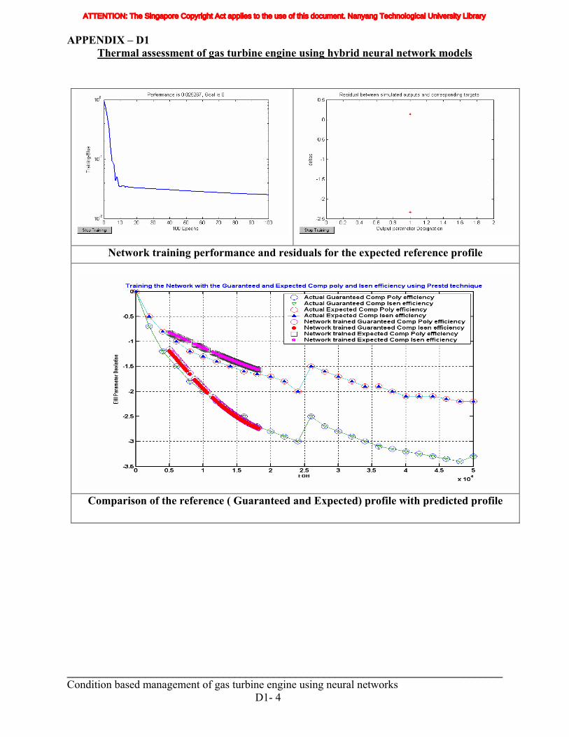
APPENDIX – D1 Thermal assessment of gas turbine engine using hybrid neural network models
Network training performance and residuals for the expected reference profile
Comparison of the reference ( Guaranteed and Expected) profile with predicted profile
______________________________________________________________________________ Condition based management of gas turbine engine using neural networks D1- 4
ATTENTION: The Singapore Copyright Act applies to the use of this document. Nanyang Technological University Library
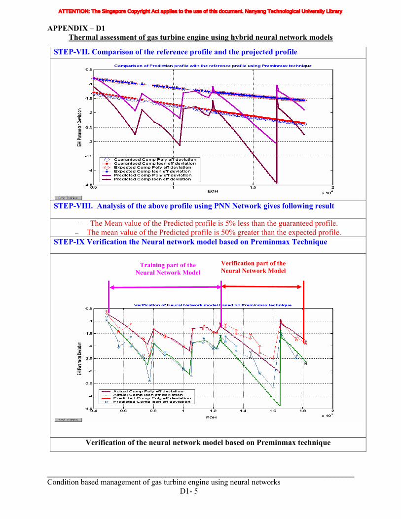
APPENDIX – D1 Thermal assessment of gas turbine engine using hybrid neural network models
STEP-VII. Comparison of the reference profile and the projected profile
STEP-VIII. Analysis of the above profile using PNN Network gives following result
The Mean value of the Predicted profile is 5% less than the guaranteed profile. The mean value of the Predicted profile is 50% greater than the expected profile.
STEP-IX Verification the Neural network model based on Preminmax Technique
Verification of the neural network model based on Preminmax technique
– –
Verification part of the Neural Network Model
Training part of the Neural Network Model
______________________________________________________________________________ Condition based management of gas turbine engine using neural networks D1- 5
ATTENTION: The Singapore Copyright Act applies to the use of this document. Nanyang Technological University Library
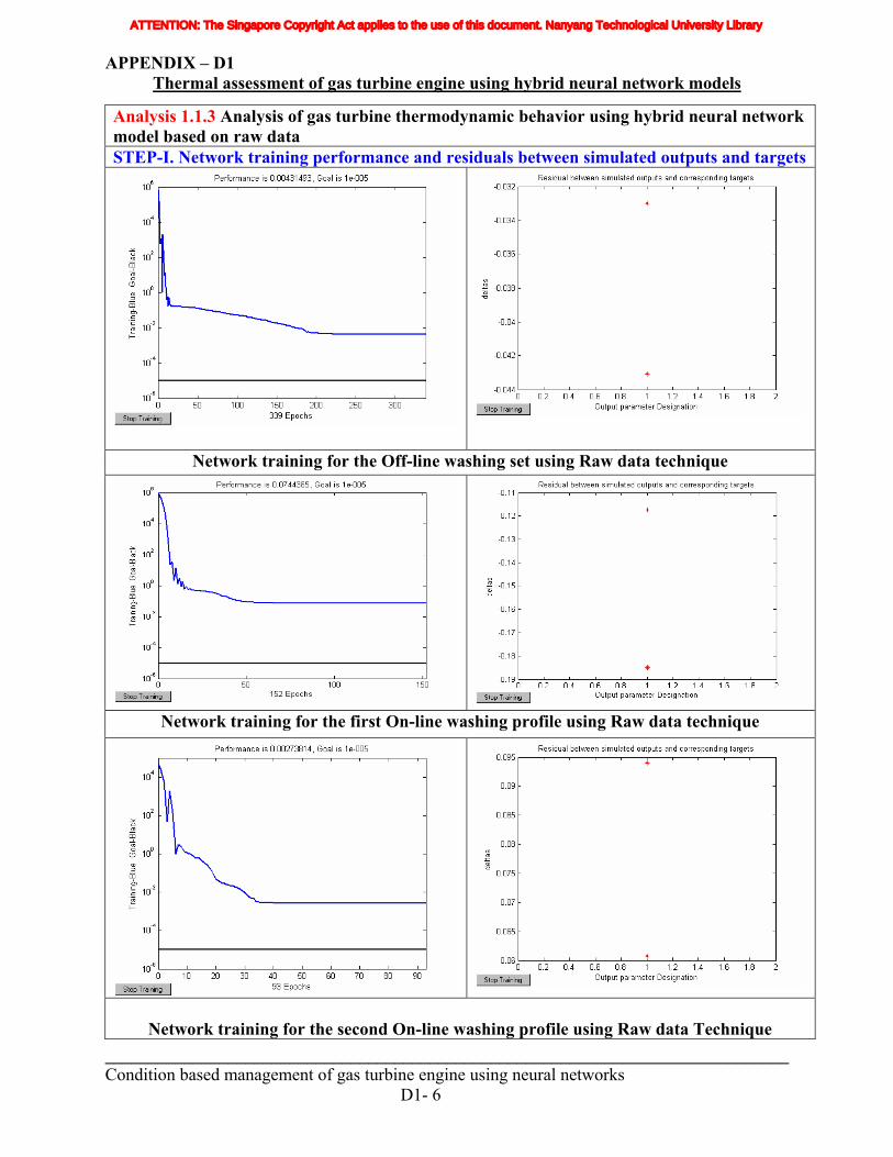
APPENDIX – D1 Thermal assessment of gas turbine engine using hybrid neural network models
Analysis 1.1.3 Analysis of gas turbine thermodynamic behavior using hybrid neural network model based on raw data STEP-I. Network training performance and residuals between simulated outputs and targets
Network training for the Off-line washing set using Raw data technique
Network training for the first On-line washing profile using Raw data technique
Network training for the second On-line washing profile using Raw data Technique
______________________________________________________________________________ Condition based management of gas turbine engine using neural networks D1- 6
ATTENTION: The Singapore Copyright Act applies to the use of this document. Nanyang Technological University Library
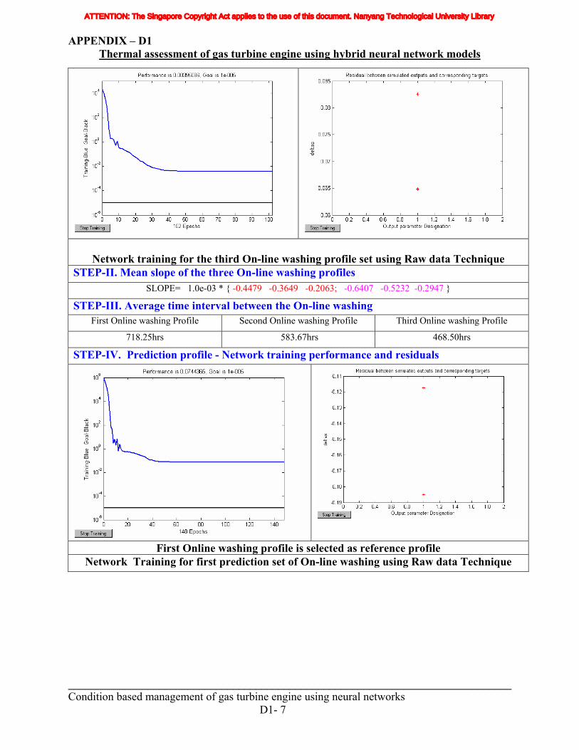
APPENDIX – D1 Thermal assessment of gas turbine engine using hybrid neural network models
Network training for the third On-line washing profile set using Raw data Technique
STEP-II. Mean slope of the three On-line washing profiles SLOPE= 1.0e-03 * { -0.4479 -0.3649 -0.2063; -0.6407 -0.5232 -0.2947 }
STEP-III. Average time interval between the On-line washing First Online washing Profile Second Online washing Profile Third Online washing Profile
718.25hrs 583.67hrs 468.50hrs
STEP-IV. Prediction profile - Network training performance and residuals
First Online washing profile is selected as reference profile Network Training for first prediction set of On-line washing using Raw data Technique
______________________________________________________________________________ Condition based management of gas turbine engine using neural networks D1- 7
ATTENTION: The Singapore Copyright Act applies to the use of this document. Nanyang Technological University Library
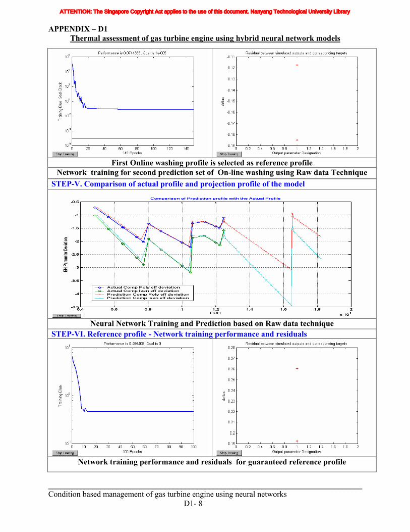
APPENDIX – D1 Thermal assessment of gas turbine engine using hybrid neural network models
First Online washing profile is selected as reference profile
Network training for second prediction set of On-line washing using Raw data Technique STEP-V. Comparison of actual profile and projection profile of the model
Neural Network Training and Prediction based on Raw data technique
STEP-VI. Reference profile - Network training performance and residuals
Network training performance and residuals for guaranteed reference profile
______________________________________________________________________________ Condition based management of gas turbine engine using neural networks D1- 8
ATTENTION: The Singapore Copyright Act applies to the use of this document. Nanyang Technological University Library
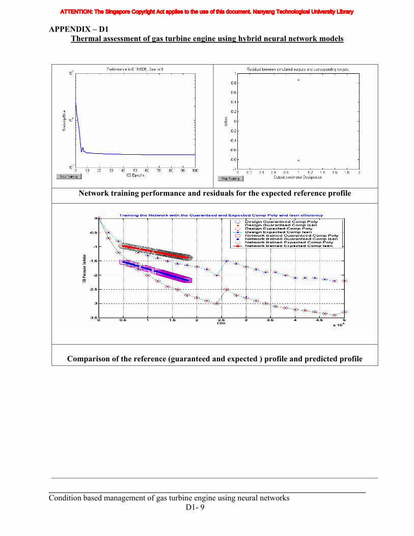
APPENDIX – D1 Thermal assessment of gas turbine engine using hybrid neural network models
Network training performance and residuals for the expected reference profile
Comparison of the reference (guaranteed and expected ) profile and predicted profile
______________________________________________________________________________ Condition based management of gas turbine engine using neural networks D1- 9
ATTENTION: The Singapore Copyright Act applies to the use of this document. Nanyang Technological University Library
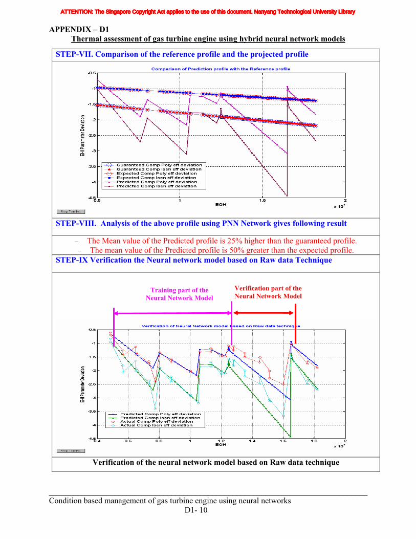
APPENDIX – D1 Thermal assessment of gas turbine engine using hybrid neural network models
______________________________________________________________________________ Condition based management of gas turbine engine using neural networks D1- 10
STEP-VII. Comparison of the reference profile and the projected profile
STEP-VIII. Analysis of the above profile using PNN Network gives following result
The Mean value of the Predicted profile is 25% higher than the guaranteed profile. The mean value of the Predicted profile is 50% greater than the expected profile.
STEP-IX Verification the Neural network model based on Raw data Technique
Verification of the neural network model based on Raw data technique
– –
Verification part of the Neural Network Model
Training part of the Neural Network Model
ATTENTION: The Singapore Copyright Act applies to the use of this document. Nanyang Technological University Library
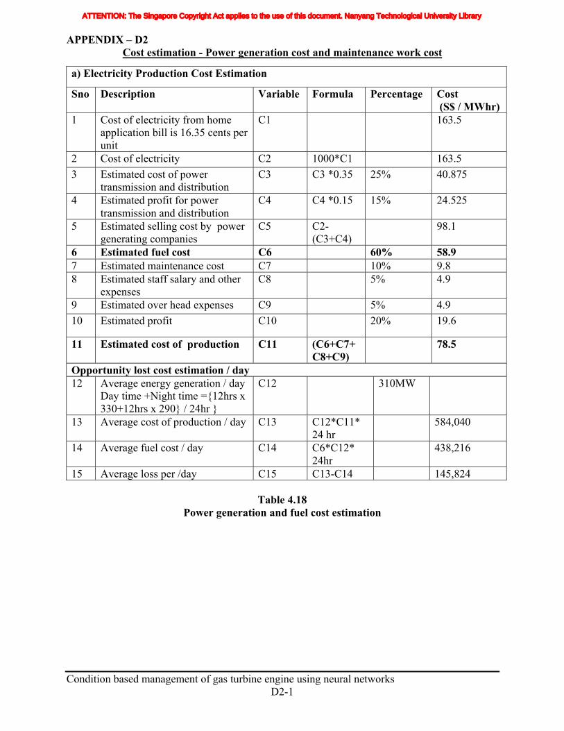
APPENDIX – D2 Cost estimation - Power generation cost and maintenance work cost
a) Electricity Production Cost Estimation
Sno Description Variable Formula Percentage Cost (S$ / MWhr)
1 Cost of electricity from home application bill is 16.35 cents per unit
C1 163.5
2 Cost of electricity C2 1000*C1 163.5 3 Estimated cost of power
transmission and distribution C3 C3 *0.35 25% 40.875
4 Estimated profit for power transmission and distribution
C4 C4 *0.15 15% 24.525
5 Estimated selling cost by power generating companies
C5 C2-(C3+C4)
98.1
6 Estimated fuel cost C6 60% 58.9 7 Estimated maintenance cost C7 10% 9.8 8 Estimated staff salary and other
expenses C8 5% 4.9
9 Estimated over head expenses C9 5% 4.9 10 Estimated profit C10 20% 19.6
11 Estimated cost of production C11 (C6+C7+C8+C9)
78.5
Opportunity lost cost estimation / day 12 Average energy generation / day
Day time +Night time ={12hrs x 330+12hrs x 290} / 24hr }
C12 310MW
13 Average cost of production / day
C13 C12*C11* 24 hr
584,040
14 Average fuel cost / day C14 C6*C12* 24hr
438,216
15 Average loss per /day C15 C13-C14 145,824
Table 4.18 Power generation and fuel cost estimation
Condition based management of gas turbine engine using neural networks
D2-1
ATTENTION: The Singapore Copyright Act applies to the use of this document. Nanyang Technological University Library
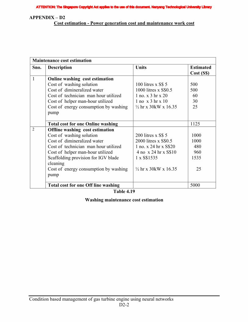
APPENDIX – D2 Cost estimation - Power generation cost and maintenance work cost
Condition based management of gas turbine engine using neural networks
D2-2
Maintenance cost estimation Sno. Description Units Estimated
Cost (S$) Online washing cost estimation Cost of washing solution Cost of dimineralized water Cost of technician man hour utilized Cost of helper man-hour utilized Cost of energy consumption by washing pump
100 litres x S$ 5 1000 litres x S$0.5 1 no. x 3 hr x 20 1 no x 3 hr x 10 ½ hr x 30kW x 16.35
500 500 60 30 25
1
Total cost for one Online washing 1125 Offline washing cost estimation Cost of washing solution Cost of dimineralized water Cost of technician man hour utilized Cost of helper man-hour utilized Scaffolding provision for IGV blade cleaning Cost of energy consumption by washing pump
200 litres x S$ 5 2000 litres x S$0.5 1 no. x 24 hr x S$20 4 no x 24 hr x S$10 1 x S$1535 ½ hr x 30kW x 16.35
1000 1000 480 960 1535 25
2
Total cost for one Off line washing 5000 Table 4.19
Washing maintenance cost estimation
ATTENTION: The Singapore Copyright Act applies to the use of this document. Nanyang Technological University Library