Concepts in

Edge Detection

Dr. Sukhendu DasDeptt. of Computer Science and Engg.,Indian Institute of Technology, Madras

Chennai – 600036, India.

http://www.cs.iitm.ernet.in/~sdasEmail: sdas@iitm.ac.in

Edge DetectionEdge is a boundary between two homogeneous regions. The

gray level properties of the two regions on either side of an edge are distinct and exhibit some local uniformity or homogeneity among themselves.

An edge is typically extracted by computing the derivative of the image intensity function. This consists of two parts:

• Magnitude of the derivative: measure of the strength/contrast ofthe edge

• Direction of the derivative vector: edge orientation

Ideal Step edge in 1-D Step edge in 2-D

Computing the derivative: Finite difference in 1-D

22

2 )()(2)(

2)()()()(

dxdxxfxfdxxf

xdfd

dxdxxfdxxf

dxxfdxxf

dxdf

−+−+≈

−−+≈

−+≈

x-dx x x+dx X

F(x)

Computing the derivative: Finite differences in 2-D

dydyyxfdyyxf

dyyxfdyyxf

yf

dxdydxxfdydxxf

dxyxfydxxf

xf

2),(),(),(),(

2),(),(),(),(

−−+≈

−+≈

∂∂

−−+≈

−+≈

∂∂

Original Image Horizontal derivative Vertical derivative

Differentiation using convolution:

δf/δx = [-1 1]; δf/δy = [-1 1]T ;

δ2f/δx2 = [1 -2 1]; δ2f/δy2 = [1 -2 1]T ;

Need to use wider masks to add an element of smoothing and better response. The traditional derivative operators used were:

Roberts

Prewitt

Sobel

⎥⎥⎥

⎦

⎤

⎢⎢⎢

⎣

⎡

−⎥⎥⎥

⎦

⎤

⎢⎢⎢

⎣

⎡

−−−

⎥⎥⎥

⎦

⎤

⎢⎢⎢

⎣

⎡

−−−⎥⎥⎥

⎦

⎤

⎢⎢⎢

⎣

⎡

−−−

⎥⎦

⎤⎢⎣

⎡−⎥

⎦

⎤⎢⎣

⎡−

121000121

,101202101

111000111

,101101101

1001

,0110

Laplacian

⎥⎥⎥

⎦

⎤

⎢⎢⎢

⎣

⎡−

010141010

Most of these partial derivative operators are sensitive to noise. Use of these masks resulted in thick edges or boundaries, in addition to spurious edge pixels due to noise.

Laplacian mask is highly sensitive to spike noise. Use of noise smoothing became mandatory before edge detection, specifically for noisy images. But noise smoothing, typically by the use of a Gaussianfunction, caused a blurring or smearing of the edge information or gradient values.

Two components of the edge values computed are:

Gradient values: Gx = δf/δx; Gy = δf/δy.

The magnitude of the edge is calculated as:

|G| = [Gx2 + Gy

2]1/2

and orientation as:

θ = arctan(Gy/Gx)

Gx, Gy

Gaussian Function

2

2

2

21)( σ

σπ

x

exg−

=

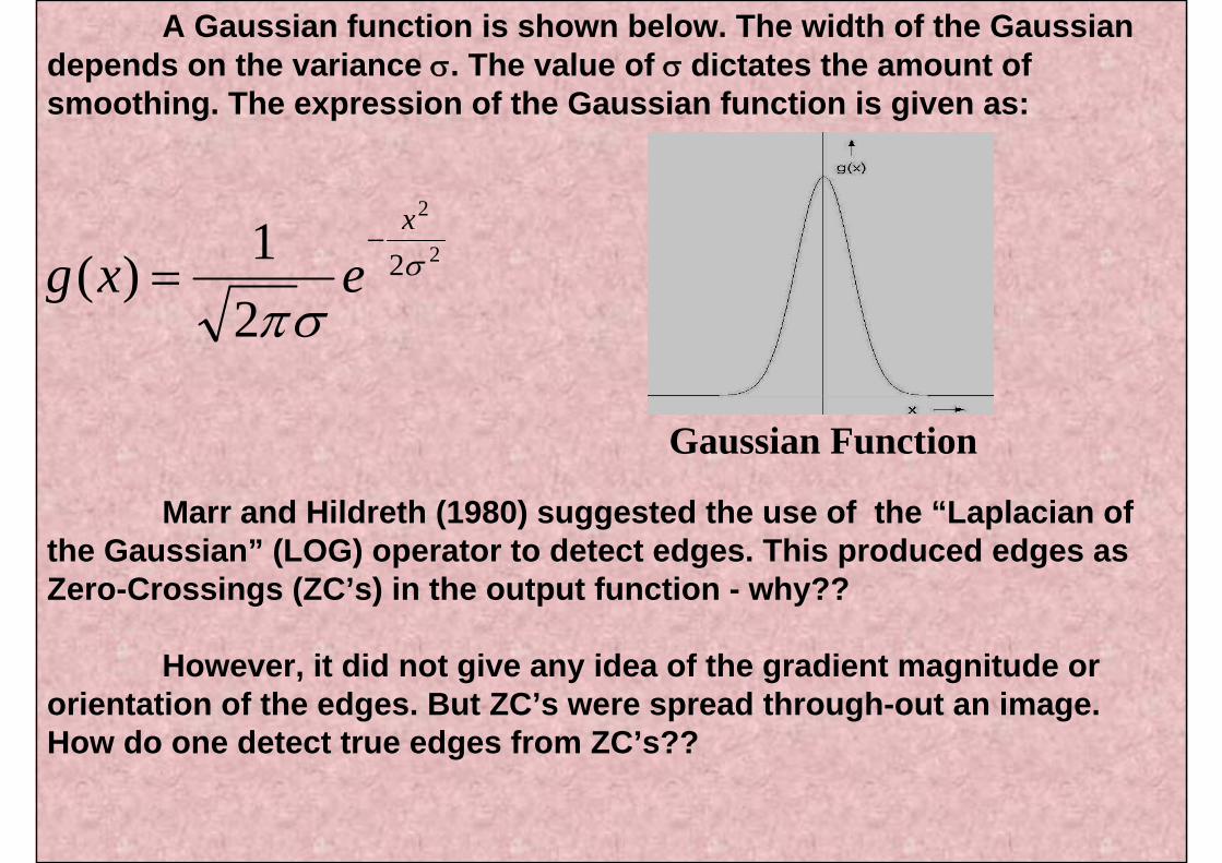
A Gaussian function is shown below. The width of the Gaussian depends on the variance σ. The value of σ dictates the amount of smoothing. The expression of the Gaussian function is given as:

Marr and Hildreth (1980) suggested the use of the “Laplacian of the Gaussian” (LOG) operator to detect edges. This produced edges as Zero-Crossings (ZC’s) in the output function - why??

However, it did not give any idea of the gradient magnitude or orientation of the edges. But ZC’s were spread through-out an image. How do one detect true edges from ZC’s??

LOG operator in 1-D

LOG operator in 2-D

First Derivative

IdealStepEdge

SmoothedStepEdge

G:Gaussian Function

Images

HorizontalIntensityProfiles

FirstDerivative

Second Derivative

Edge NoisyEdge

First Derivative Second Derivative

)2

exp()2

()(')( 2

2

3 σσπyyygyc −−

==

Canny in 1986 suggested an optimal operator, which uses the Gaussian smoothing and the derivative function together. He proved that the first derivative of the Gaussian function, as shown below, is a good approximation to his optimal operator.

It combines both the derivative and smoothing properties in a nice way to obtain good edges. Canny also talks of a hysteresis basedthresholding strategy for marking the edges from the gradient values.

Smoothing and derivative when applied separately, were not producing good results under noisy conditions. This is because, one opposes the other. Whereas, when combined together produces the desired output.

Expression of Canny (1-D operator is):

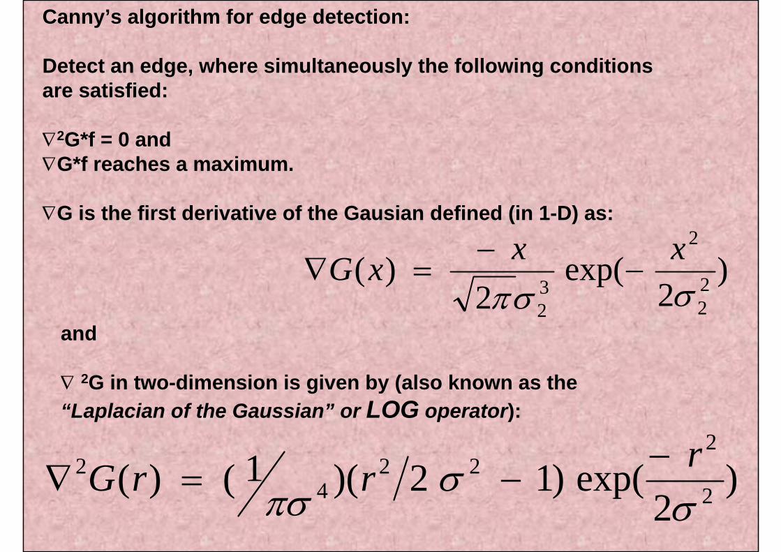
Canny’s algorithm for edge detection:

Detect an edge, where simultaneously the following conditions are satisfied:

∇2G*f = 0 and ∇G*f reaches a maximum.

∇G is the first derivative of the Gausian defined (in 1-D) as:

)2

exp(2

)( 22

2

32 σσπ

xxxG −−

=∇

and

∇ 2G in two-dimension is given by (also known as the“Laplacian of the Gaussian” or LOG operator):

)2

exp()12)(1()( 2

222

42

σσπσ

rrrG −−=∇

NoisyEdge, Sn

G:Gaussian Function

δG δG * Sn

δG

δ2G

δG * Sn

δ2G * Sn

NoisyEdge, Sn

δG

δ2G

δG * Sn

δ2G * Sn

Original Gray scale Image X-gradient Y-gradient Total Gradient

MagnitudeBi level

Thresholding

Original Grey level Image After Laplace Operator After Zero-crossing

Lena

LOG

Sobel

Canny

Venice

LOG

Sobel

Canny

BIRD SOBEL

LOG Canny

Multi-scale Edge detection

• Our goal is to simultaneously extract edges of all lengths

• Edges are well localized across the scale-space

Problem definition

Input image Edge map generated by scale space Combination

Edge map generated by single scale

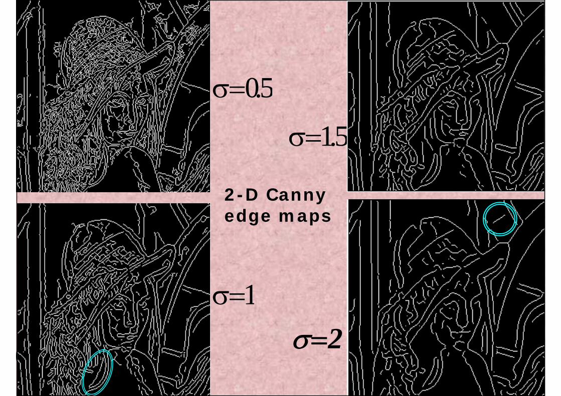
5.0=σ

2=σ1=σ

5.1=σ

2-D Canny edge maps

• Real-world objects are composed of different structures at different scales

Motivation

• Connectivity of an object depends on the scale at which it is observed

• In real-world images the edges may not be ideal

• Variation of the response over different scales is important

• A step edge is sensed at various points by cells of the retinal array

Optimal Edge Detection in Two-Dimensional Images

NES: Normalized Edge Strength

NESS: Normalized Edge Strength of sub-segment

LT: Low Threshold

HT: High threshold

MT: Medium Threshold

Compute the gradient map of Gaussian blurred image.

Assign the magnitude of the gradient as edge strength to all edge pixels.

Edge strength is equalized (HEQ) to full scale of intensity.

Compute the normalized edge strength (NES) for all edge segments as sum of strengths of all the edge points divided by length of the segment.

Compute the histogram for the edge segment strengths.

Fit a Gaussian to the low intensity part of the histogram and compute three threshold (Low, medium and high) based on mean and variance of Gaussian.

NES > MT

Salient edge Map

yes

No yes

Compute edge subsegments and compute NESS for each subsegment.

NESS >LT

NESS > HT yes

SALIENCY TEST

Histogram of the normalised edge strengths and fitted Gaussian distribution

5.0=σ

5.1=σ

5.0=σ 2=σ1=σ

Salient Edge maps

5.1=σ

2-D Canny edge map

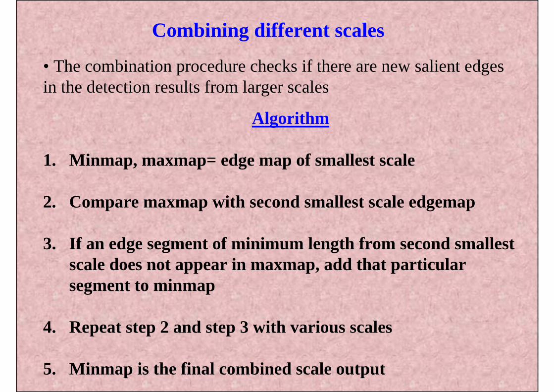
• The combination procedure checks if there are new salient edgesin the detection results from larger scales

Algorithm

1. Minmap, maxmap= edge map of smallest scale

2. Compare maxmap with second smallest scale edgemap

3. If an edge segment of minimum length from second smallest scale does not appear in maxmap, add that particular segment to minmap

4. Repeat step 2 and step 3 with various scales

5. Minmap is the final combined scale output

Combining different scales

Scale space combination2-D Canny edge model

Scale space combinationof Qian & Huang

edge model

Lena256x256

REFERENCES

“Digital Image Processing and Computer Vision”; Robert J. Schallkoff; John Wiley and Sons; 1989+.

“Digital Image Processing”; R. C. Gonzalez and R. E. Woods; Addison Wesley; 1992+.

Optimal Edge Detection in Two-Dimensional Images, Richard J. Qian and Thomas S. Huang, IEEE TRANSACTIONS ON IMAGE PROCESSING, VOL. 5, NO. 7, JULY 1996, 1215-1220.

A Two-Dimensional Edge Detection Scheme for General Visual Processing , Qian, R.J. and Huang, T.S, ICPR-94, YEAR = "1994", "595-598".