Embed Size (px)
Citation preview
CSE 252A, Fall 2019 Computer Vision I
Edge Detection and Corner Detection
Computer Vision ICSE 252ALecture 7

CSE 252A, Fall 2019 Computer Vision I
Announcements• Homework 2 is due Oct 22, 11:59 PM• Homework 3 will be assigned on Oct 22• Reading:
– Chapter 5: Local Image Features
CSE 252A, Fall 2019 Computer Vision I
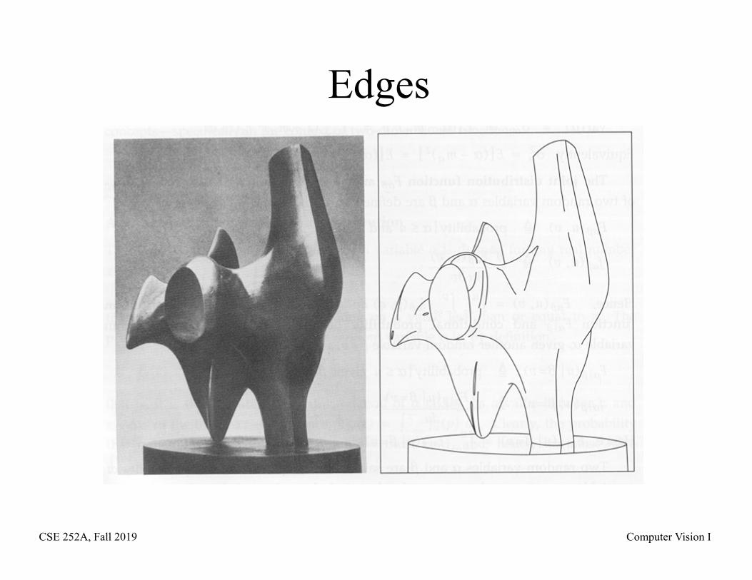
Edges
CSE 252A, Fall 2019 Computer Vision I
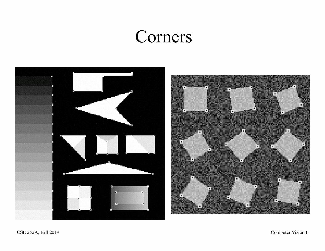
Corners
CSE 252A, Fall 2019 Computer Vision I
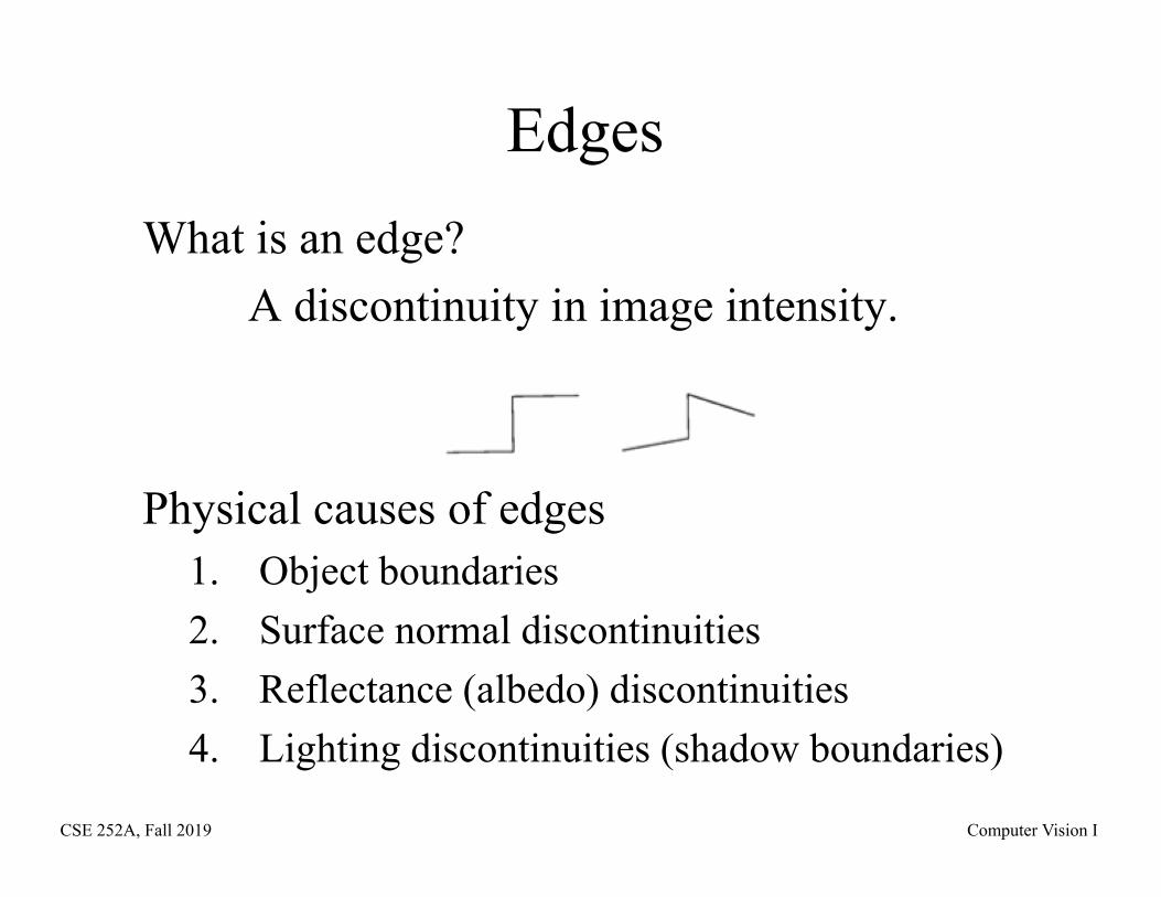
EdgesWhat is an edge?
A discontinuity in image intensity.
Physical causes of edges1. Object boundaries2. Surface normal discontinuities3. Reflectance (albedo) discontinuities4. Lighting discontinuities (shadow boundaries)
CSE 252A, Fall 2019 Computer Vision I
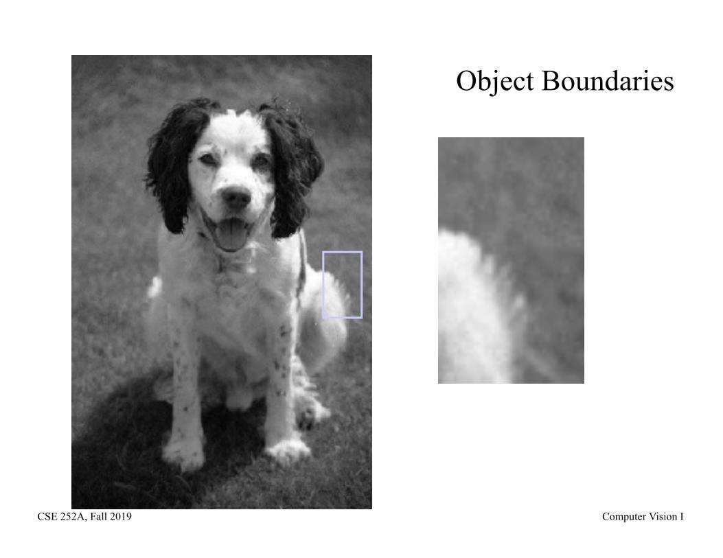
Object Boundaries
CSE 252A, Fall 2019 Computer Vision I
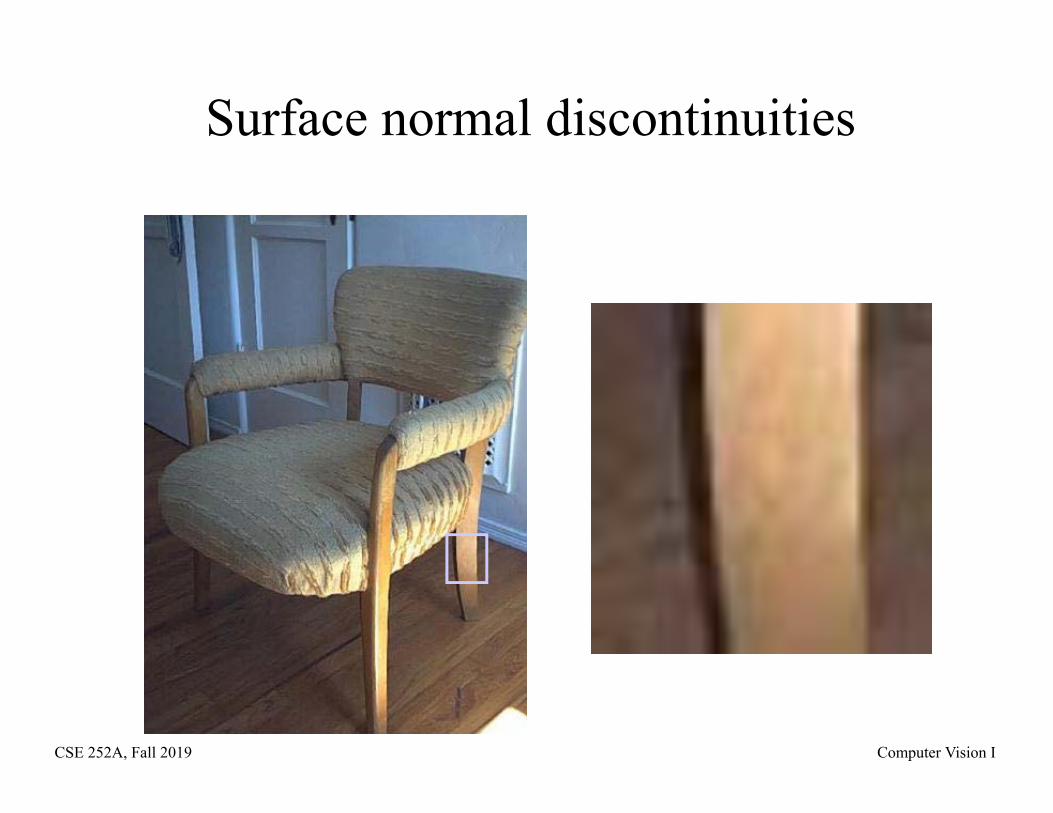
Surface normal discontinuities
CSE 252A, Fall 2019 Computer Vision I
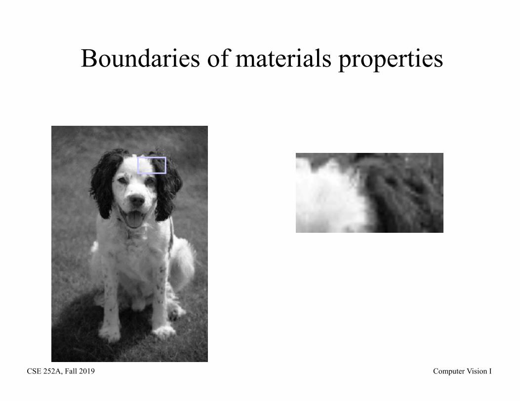
Boundaries of materials properties
CSE 252A, Fall 2019 Computer Vision I
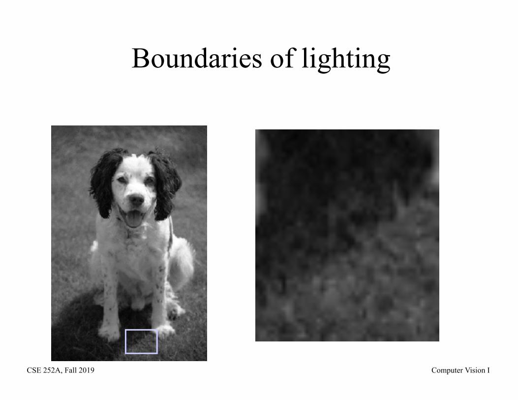
Boundaries of lighting
CSE 252A, Fall 2019 Computer Vision I
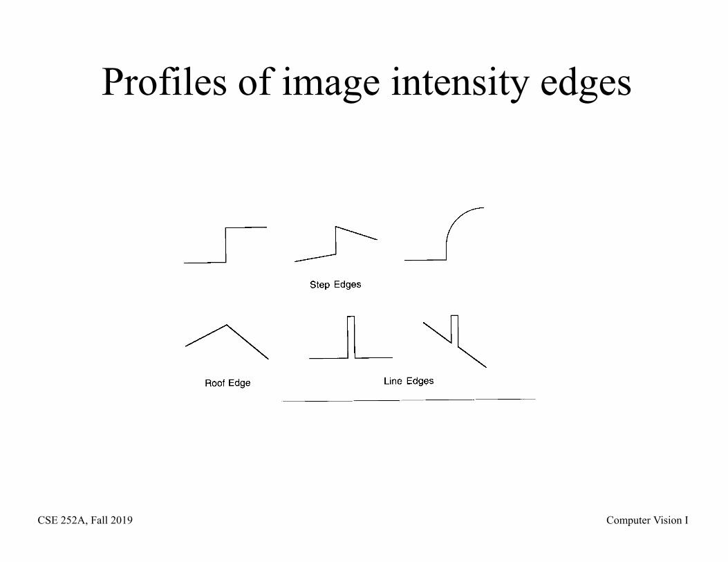
Profiles of image intensity edges
CSE 252A, Fall 2019 Computer Vision I
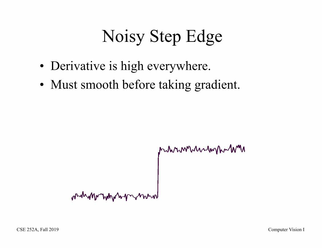
Noisy Step Edge• Derivative is high everywhere.• Must smooth before taking gradient.
CSE 252A, Fall 2019 Computer Vision I
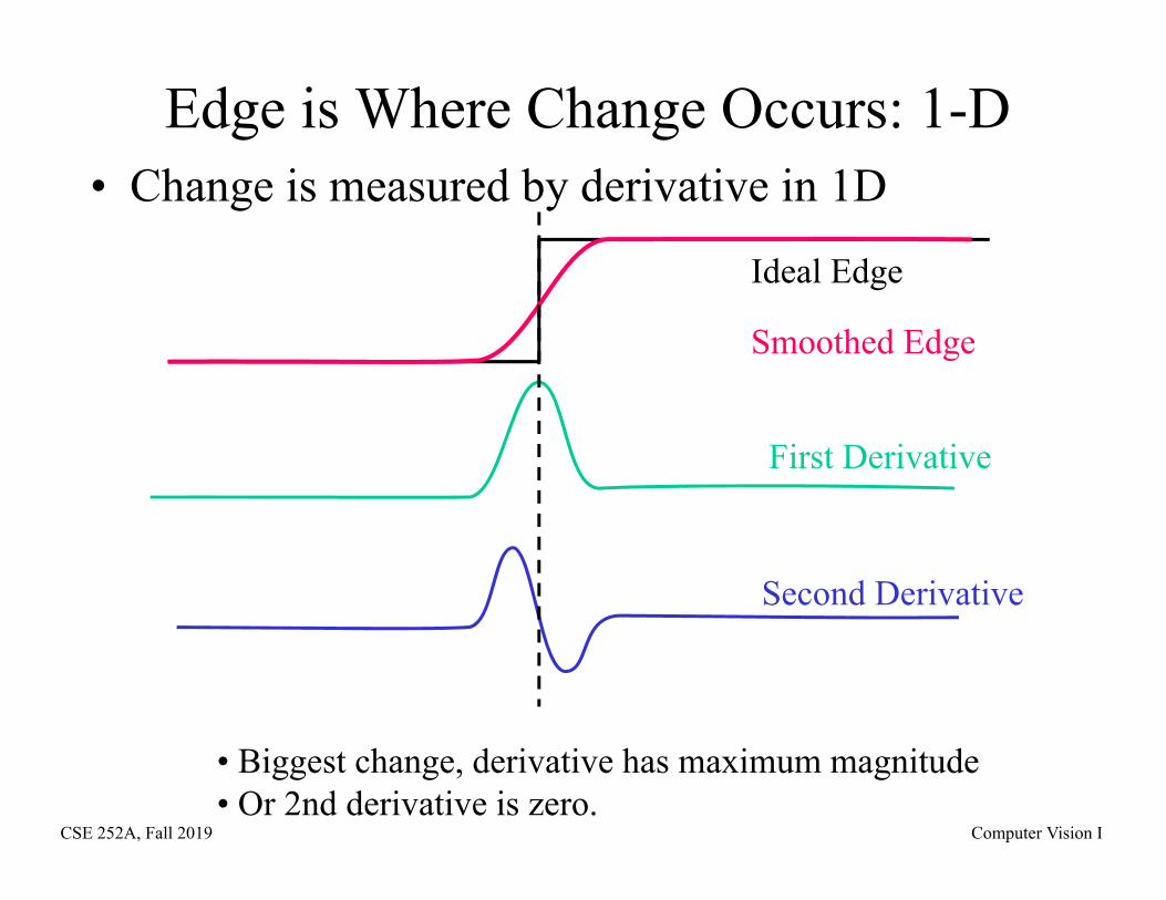
Edge is Where Change Occurs: 1-D• Change is measured by derivative in 1D
Smoothed Edge
First Derivative
Second Derivative
Ideal Edge
• Biggest change, derivative has maximum magnitude• Or 2nd derivative is zero.
CSE 252A, Fall 2019 Computer Vision I
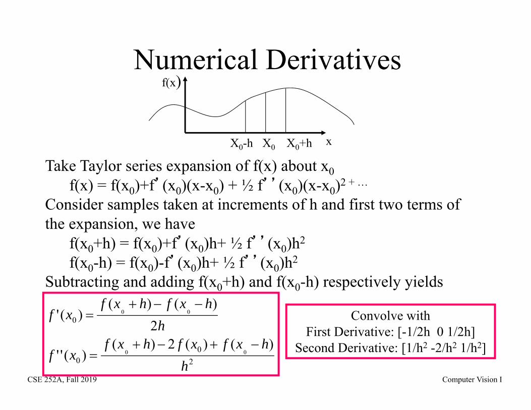
Numerical Derivativesf(x)
xX0 X0+hX0-h
Take Taylor series expansion of f(x) about x0f(x) = f(x0)+f’(x0)(x-x0) + ½ f’’(x0)(x-x0)2 + …
Consider samples taken at increments of h and first two terms of the expansion, we have
f(x0+h) = f(x0)+f’(x0)h+ ½ f’’(x0)h2
f(x0-h) = f(x0)-f’(x0)h+ ½ f’’(x0)h2
Subtracting and adding f(x0+h) and f(x0-h) respectively yields
20
0
0
)()(2)()(''
2)()(
)('
00
00
hhxfxfhxf
xf
hhxfhxf
xf
Convolve with
First Derivative: [-1/2h 0 1/2h]Second Derivative: [1/h2 -2/h2 1/h2]
CSE 252A, Fall 2019 Computer Vision I
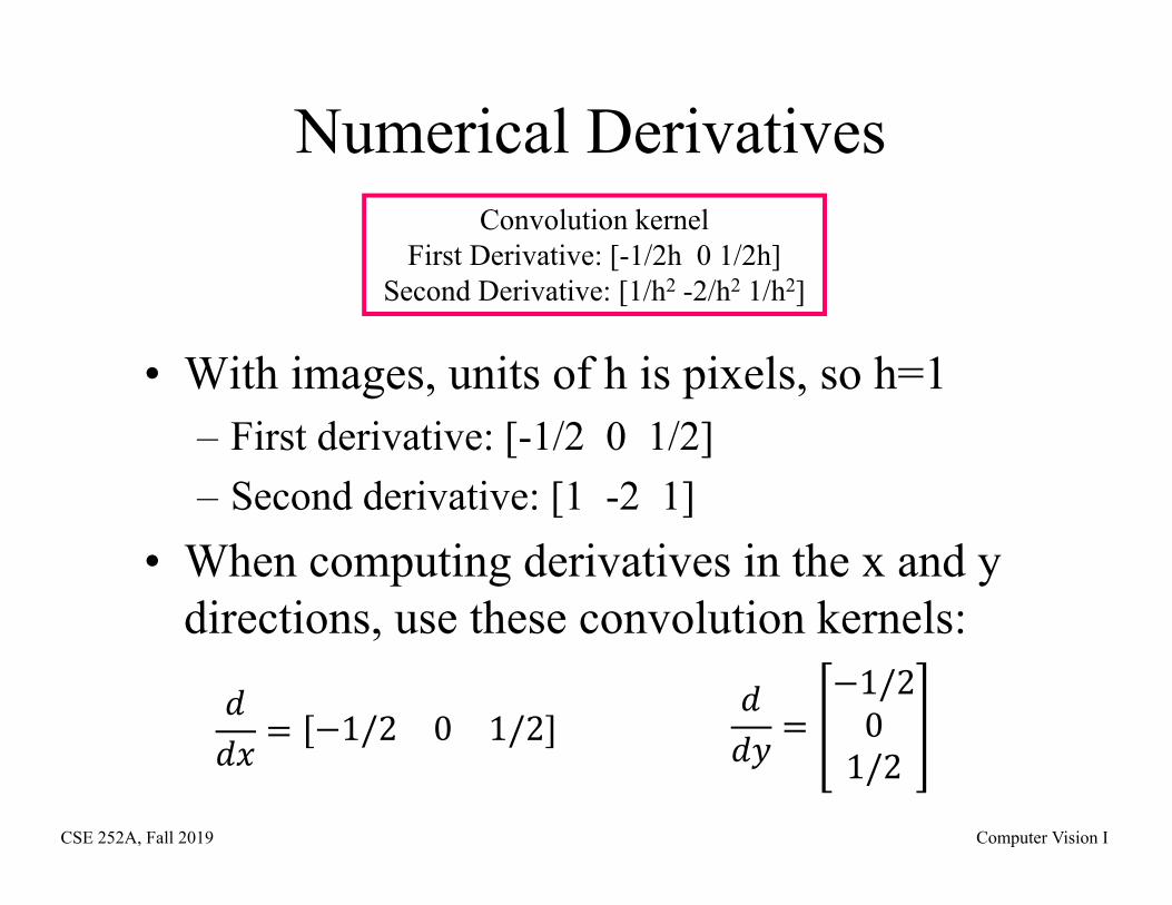
Numerical Derivatives
• With images, units of h is pixels, so h=1– First derivative: [-1/2 0 1/2]– Second derivative: [1 -2 1]
• When computing derivatives in the x and y directions, use these convolution kernels:
Convolution kernelFirst Derivative: [-1/2h 0 1/2h]
Second Derivative: [1/h2 -2/h2 1/h2]
𝑑𝑑𝑦
1/201/2
𝑑𝑑𝑥
1/2 0 1/2
CSE 252A, Fall 2019 Computer Vision I
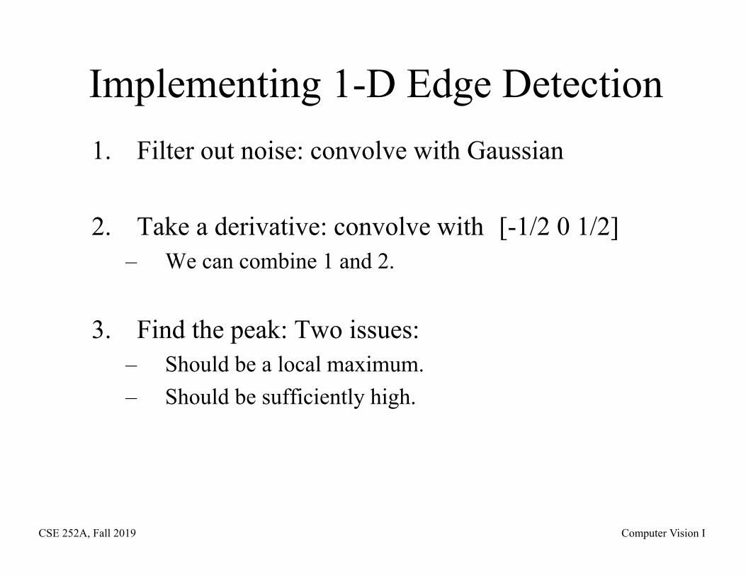
Implementing 1-D Edge Detection1. Filter out noise: convolve with Gaussian
2. Take a derivative: convolve with [-1/2 0 1/2]– We can combine 1 and 2.
3. Find the peak: Two issues:– Should be a local maximum.– Should be sufficiently high.
CSE 252A, Fall 2019 Computer Vision I
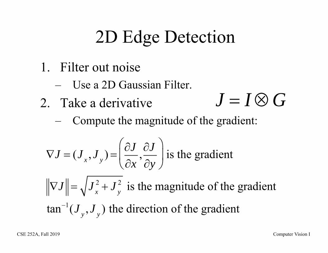
2D Edge Detection1. Filter out noise
– Use a 2D Gaussian Filter.2. Take a derivative
– Compute the magnitude of the gradient:J I G
J (J x , J y ) Jx
,Jy
is the gradient
J J x2 J y
2 is the magnitude of the gradient
tan1(J y , J y ) the direction of the gradient
CSE 252A, Fall 2019 Computer Vision I
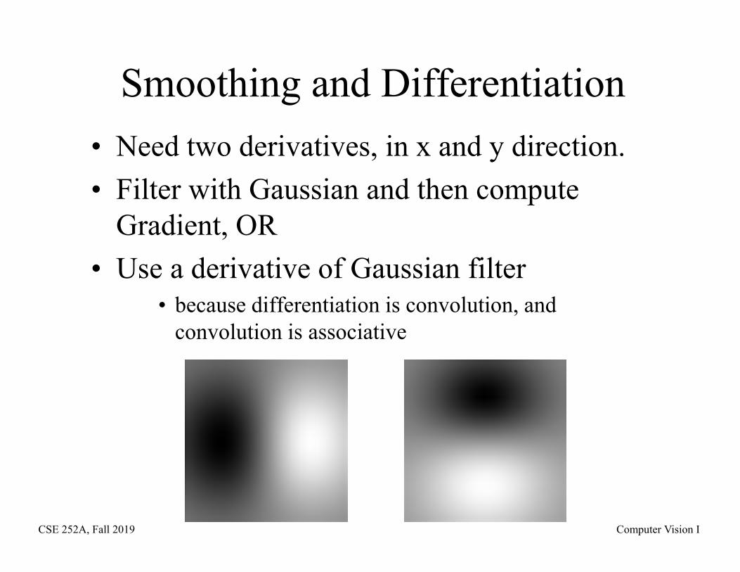
Smoothing and Differentiation• Need two derivatives, in x and y direction. • Filter with Gaussian and then compute
Gradient, OR• Use a derivative of Gaussian filter
• because differentiation is convolution, and convolution is associative
CSE 252A, Fall 2019 Computer Vision I
xG
yG
yG
xG
sincos
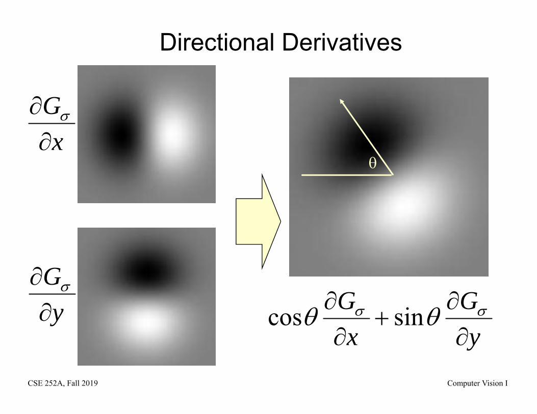
Directional Derivatives
CSE 252A, Fall 2019 Computer Vision I
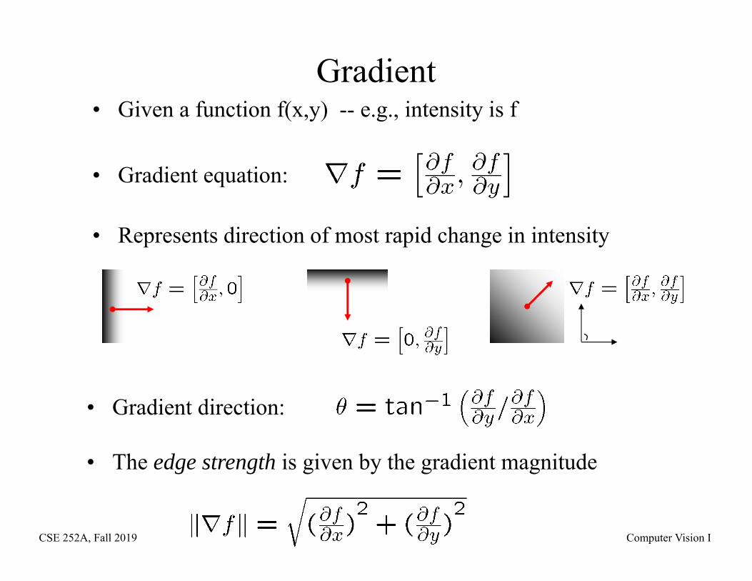
Gradient• Given a function f(x,y) -- e.g., intensity is f
• Gradient equation:
• Represents direction of most rapid change in intensity
• Gradient direction:
• The edge strength is given by the gradient magnitude
CSE 252A, Fall 2019 Computer Vision I
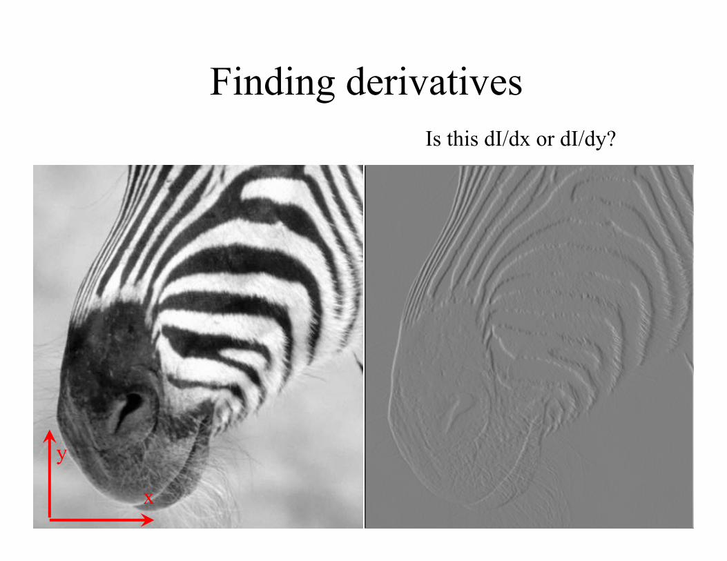
Finding derivatives
x
y
Is this dI/dx or dI/dy?
CSE 252A, Fall 2019 Computer Vision I
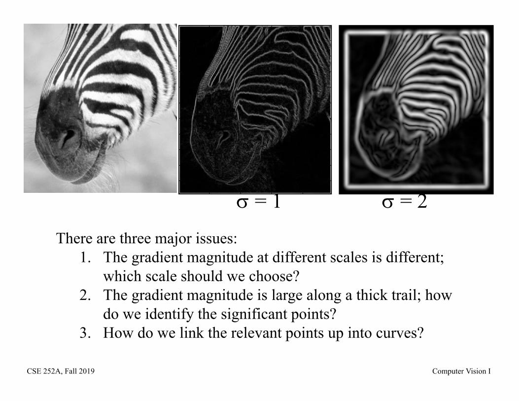
There are three major issues:1. The gradient magnitude at different scales is different;
which scale should we choose?2. The gradient magnitude is large along a thick trail; how
do we identify the significant points?3. How do we link the relevant points up into curves?
= 1 = 2
CSE 252A, Fall 2019 Computer Vision I
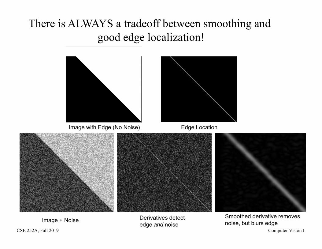
There is ALWAYS a tradeoff between smoothing and good edge localization!
Image with Edge (No Noise) Edge Location
Image + Noise Derivatives detect edge and noise
Smoothed derivative removes noise, but blurs edge
CSE 252A, Fall 2019 Computer Vision I
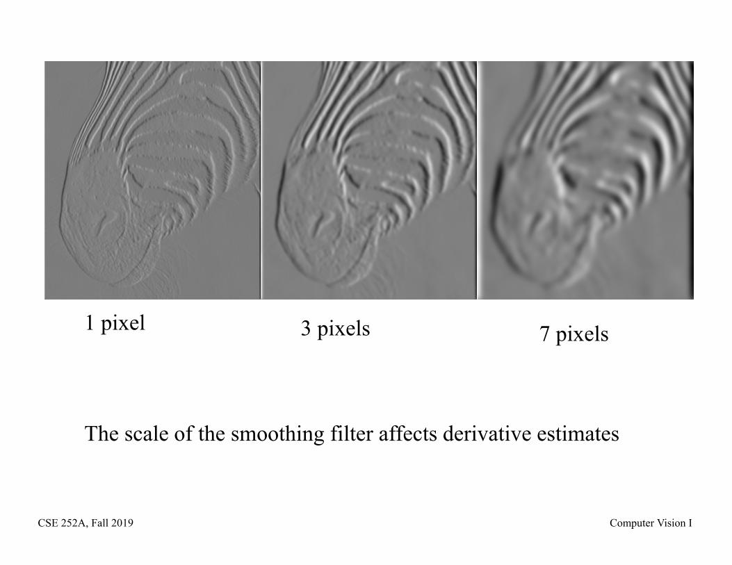
The scale of the smoothing filter affects derivative estimates
1 pixel 3 pixels 7 pixels
CSE 252A, Fall 2019 Computer Vision I
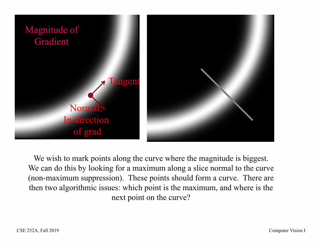
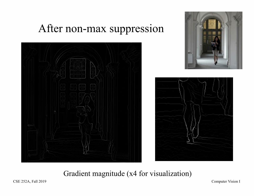
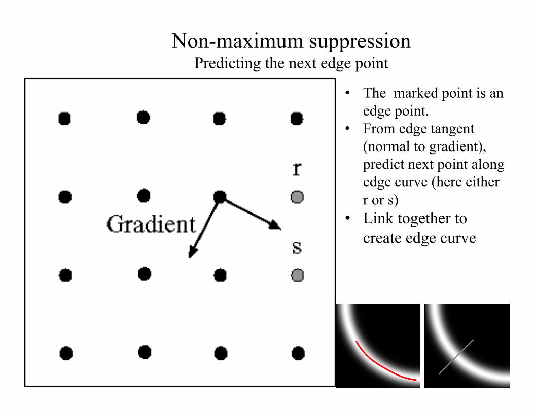
We wish to mark points along the curve where the magnitude is biggest.We can do this by looking for a maximum along a slice normal to the curve(non-maximum suppression). These points should form a curve. There arethen two algorithmic issues: which point is the maximum, and where is the
next point on the curve?
Magnitude ofGradient
Normal: In direction
of grad
Tangent
CSE 252A, Fall 2019 Computer Vision I
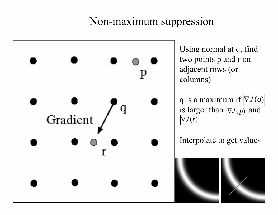
Non-maximum suppression
Using normal at q, find two points p and r on adjacent rows (or columns)
q is a maximum if is larger than and
Interpolate to get values
J (q)
J (r)J ( p)
CSE 252A, Fall 2019 Computer Vision I
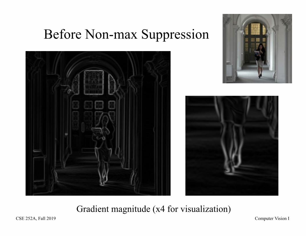
Before Non-max Suppression
Gradient magnitude (x4 for visualization)
CSE 252A, Fall 2019 Computer Vision I
After non-max suppression
Gradient magnitude (x4 for visualization)
CSE 252A, Fall 2019 Computer Vision I
• The marked point is an edge point.
• From edge tangent (normal to gradient), predict next point along edge curve (here either r or s)
• Link together to create edge curve
Non-maximum suppressionPredicting the next edge point
CSE 252A, Fall 2019 Computer Vision I
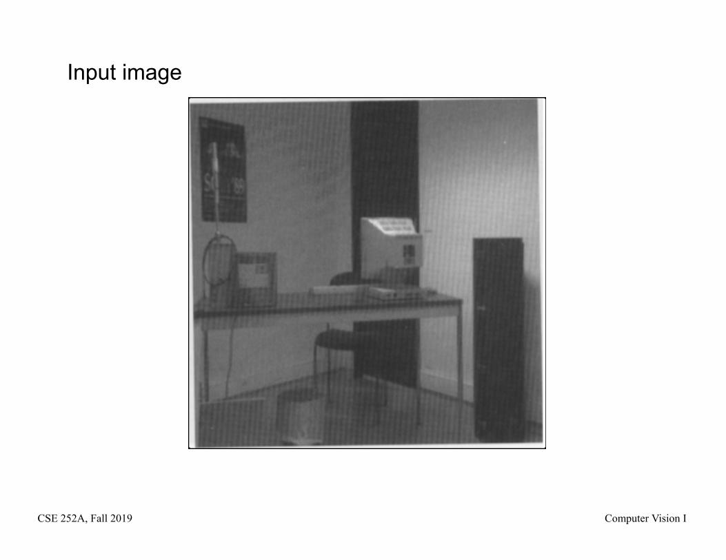
Input image
CSE 252A, Fall 2019 Computer Vision I
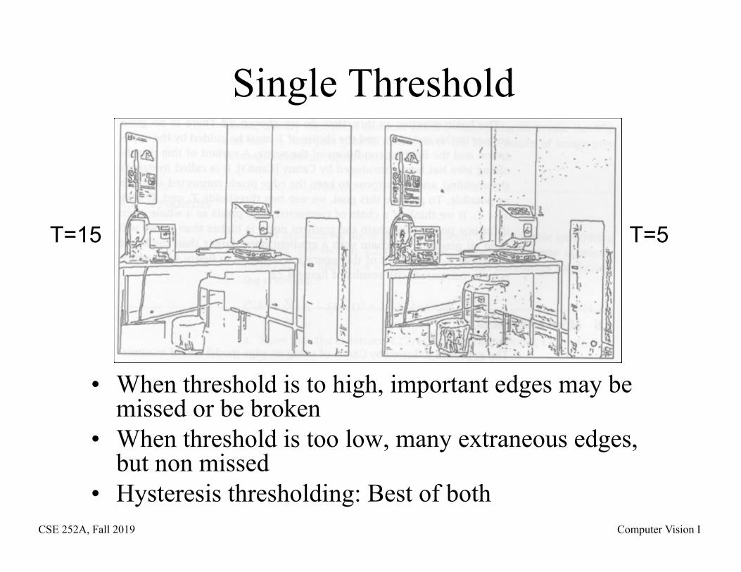
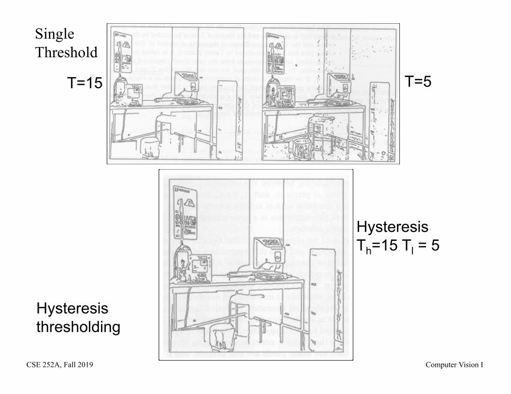
Single Threshold
• When threshold is to high, important edges may be missed or be broken
• When threshold is too low, many extraneous edges, but non missed
• Hysteresis thresholding: Best of both
T=15 T=5
CSE 252A, Fall 2019 Computer Vision I
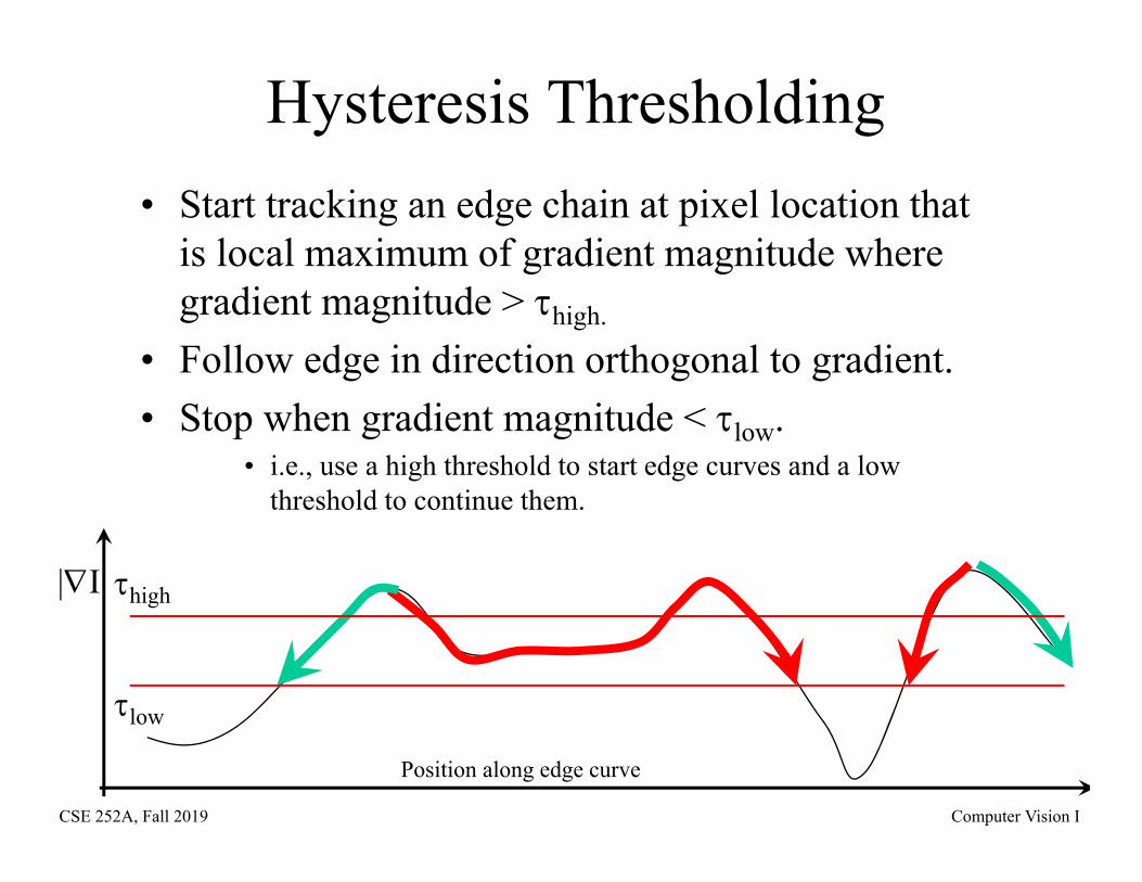
Hysteresis Thresholding• Start tracking an edge chain at pixel location that
is local maximum of gradient magnitude where gradient magnitude > high.
• Follow edge in direction orthogonal to gradient.• Stop when gradient magnitude < low.
• i.e., use a high threshold to start edge curves and a low threshold to continue them.
high
low
Position along edge curve
|I|
CSE 252A, Fall 2019 Computer Vision I
T=15 T=5
HysteresisTh=15 Tl = 5
Hysteresis thresholding
SingleThreshold
CSE 252A, Fall 2019 Computer Vision I
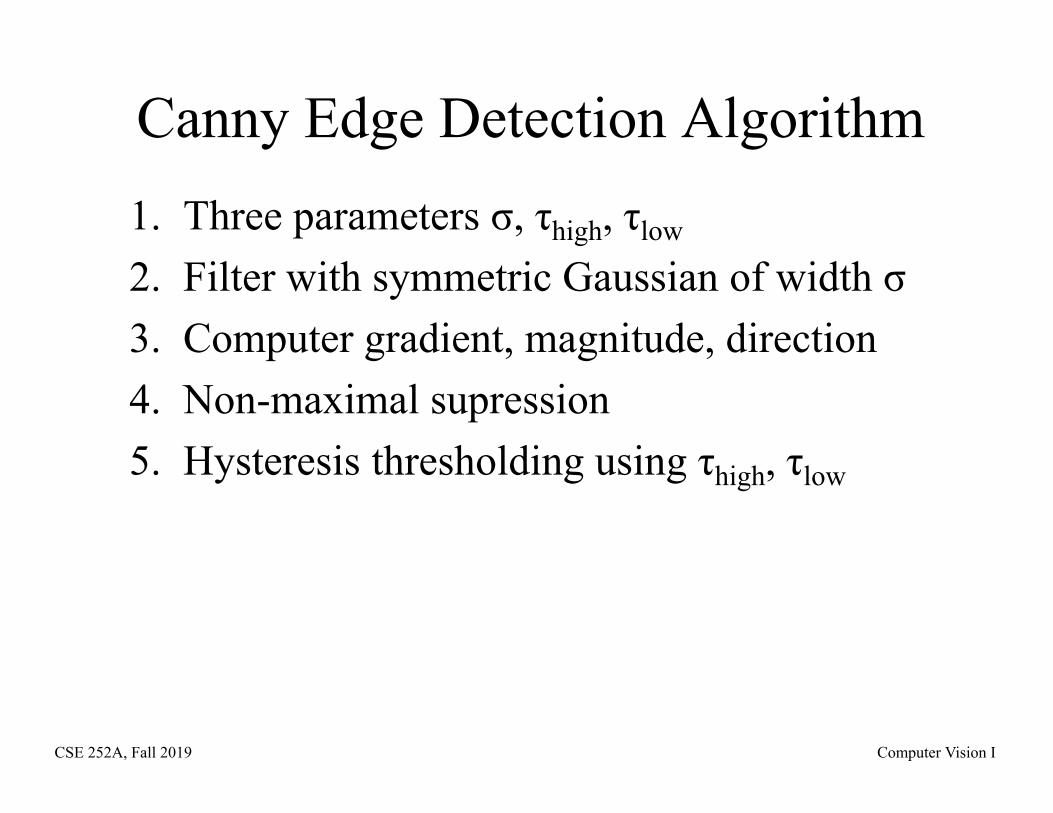
Canny Edge Detection Algorithm1. Three parameters σ, τhigh, τlow
2. Filter with symmetric Gaussian of width σ3. Computer gradient, magnitude, direction4. Non-maximal supression5. Hysteresis thresholding using τhigh, τlow
CSE 252A, Fall 2019 Computer Vision I
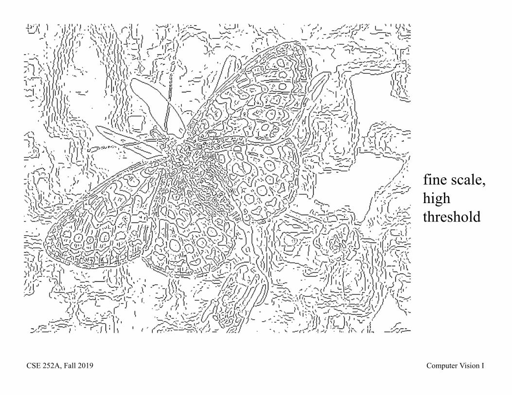
CSE 252A, Fall 2019 Computer Vision I
fine scale,high threshold
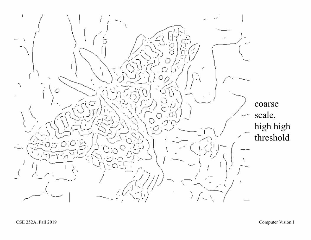
CSE 252A, Fall 2019 Computer Vision I
coarse scale,high highthreshold
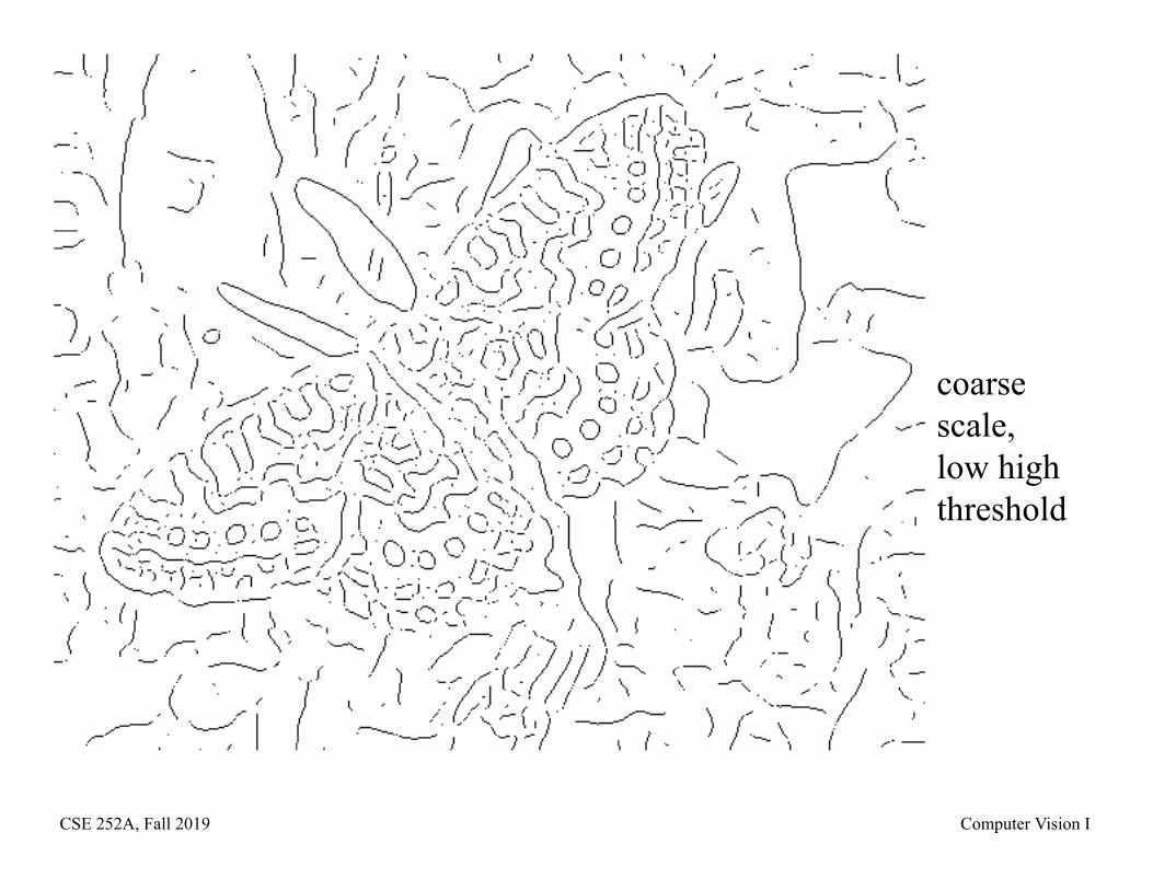
CSE 252A, Fall 2019 Computer Vision I
coarsescale,low highthreshold
CSE 252A, Fall 2019 Computer Vision I
Why is Canny so Dominant• Widely used for 30 years.• Theory is nice • Details are good
• Magnitude of gradient, • Non-max supression• Hysteresis thresholding
• Most subsequent detectors weren’t much better until learning-based detectors came along
• Code was distributed
CSE 252A, Fall 2019 Computer Vision I
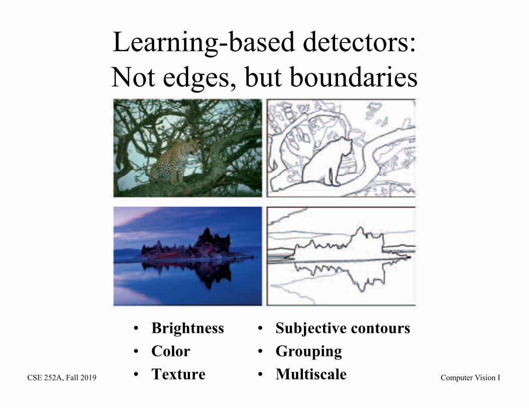
Learning-based detectors:Not edges, but boundaries
• Brightness• Color• Texture
• Subjective contours• Grouping• Multiscale
CSE 252A, Fall 2019 Computer Vision I
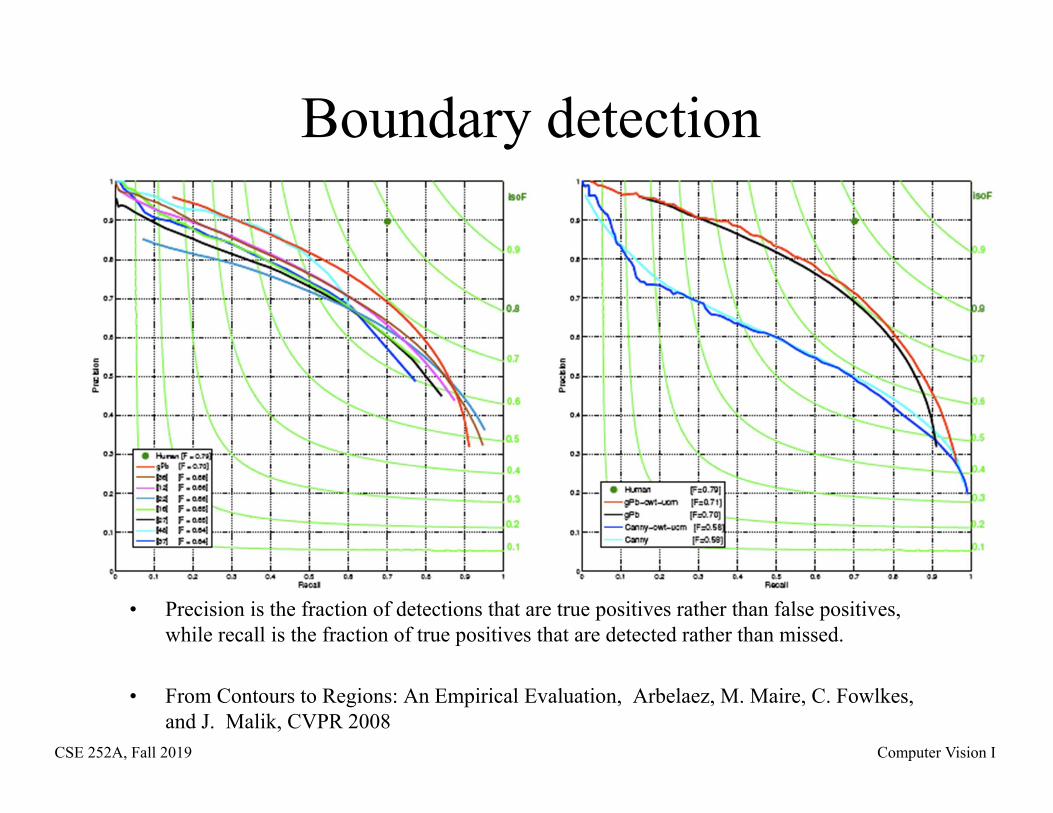
Boundary detection
• Precision is the fraction of detections that are true positives rather than false positives, while recall is the fraction of true positives that are detected rather than missed.
• From Contours to Regions: An Empirical Evaluation, Arbelaez, M. Maire, C. Fowlkes, and J. Malik, CVPR 2008
CSE 252A, Fall 2019 Computer Vision I
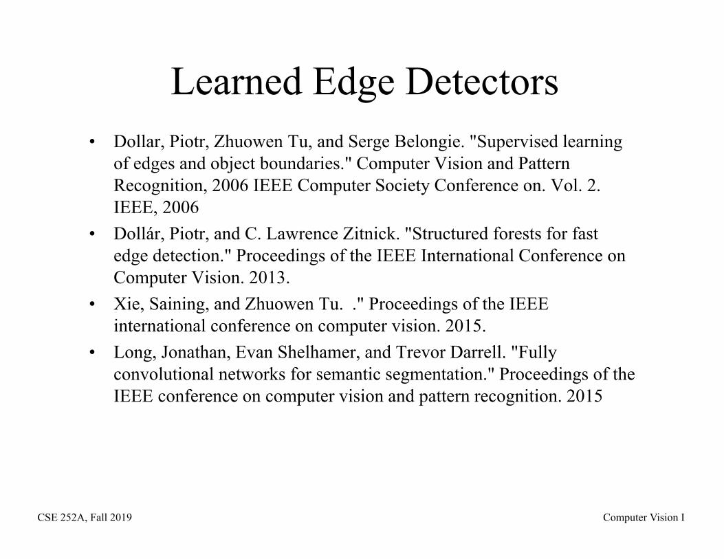
Learned Edge Detectors• Dollar, Piotr, Zhuowen Tu, and Serge Belongie. "Supervised learning
of edges and object boundaries." Computer Vision and Pattern Recognition, 2006 IEEE Computer Society Conference on. Vol. 2. IEEE, 2006
• Dollár, Piotr, and C. Lawrence Zitnick. "Structured forests for fast edge detection." Proceedings of the IEEE International Conference on Computer Vision. 2013.
• Xie, Saining, and Zhuowen Tu. ." Proceedings of the IEEE international conference on computer vision. 2015.
• Long, Jonathan, Evan Shelhamer, and Trevor Darrell. "Fully convolutional networks for semantic segmentation." Proceedings of the IEEE conference on computer vision and pattern recognition. 2015
CSE 252A, Fall 2019 Computer Vision I
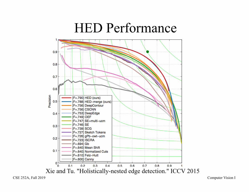
HED Performance
Xie and Tu. "Holistically-nested edge detection." ICCV 2015
CSE 252A, Fall 2019 Computer Vision I
Corner Detection
CSE 252A, Fall 2019 Computer Vision I
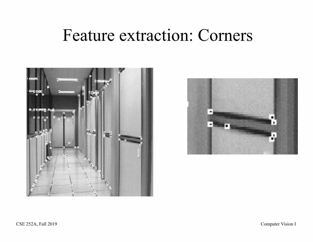
Feature extraction: Corners
CSE 252A, Fall 2019 Computer Vision I
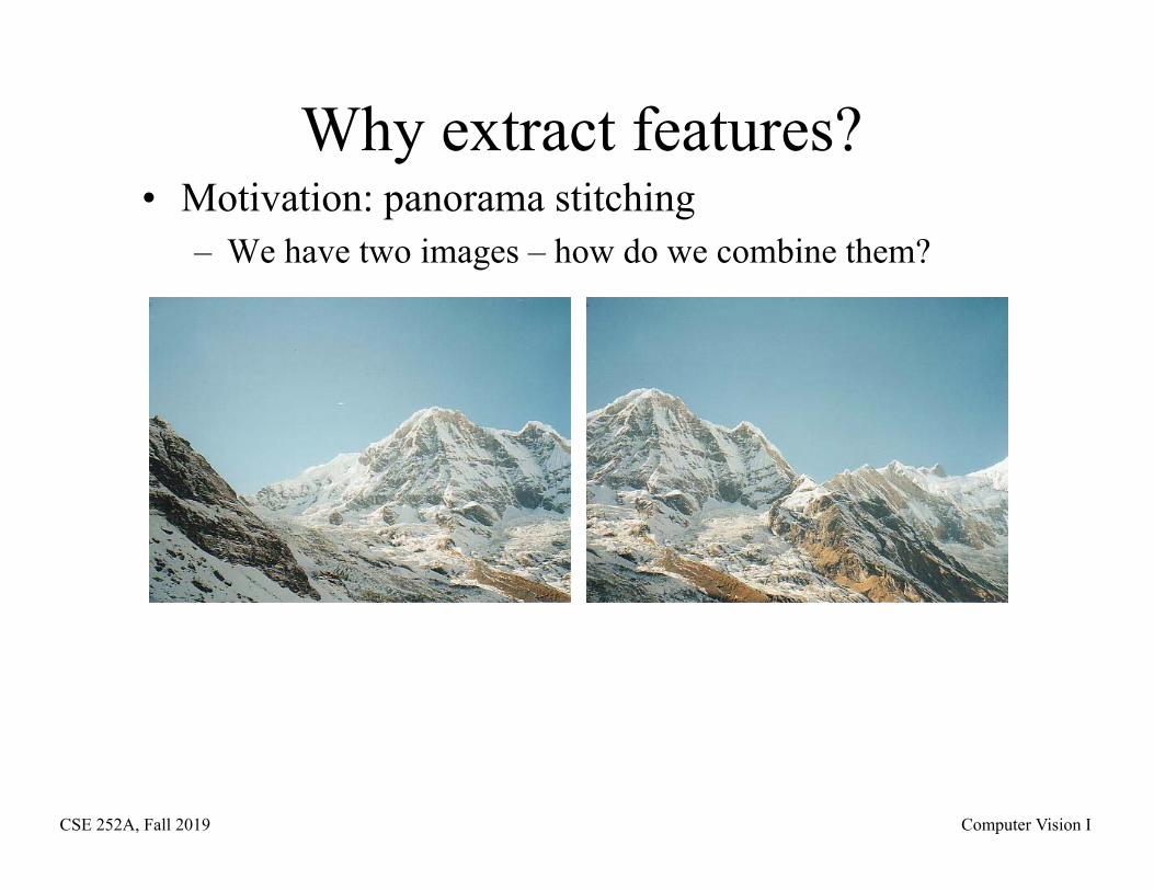
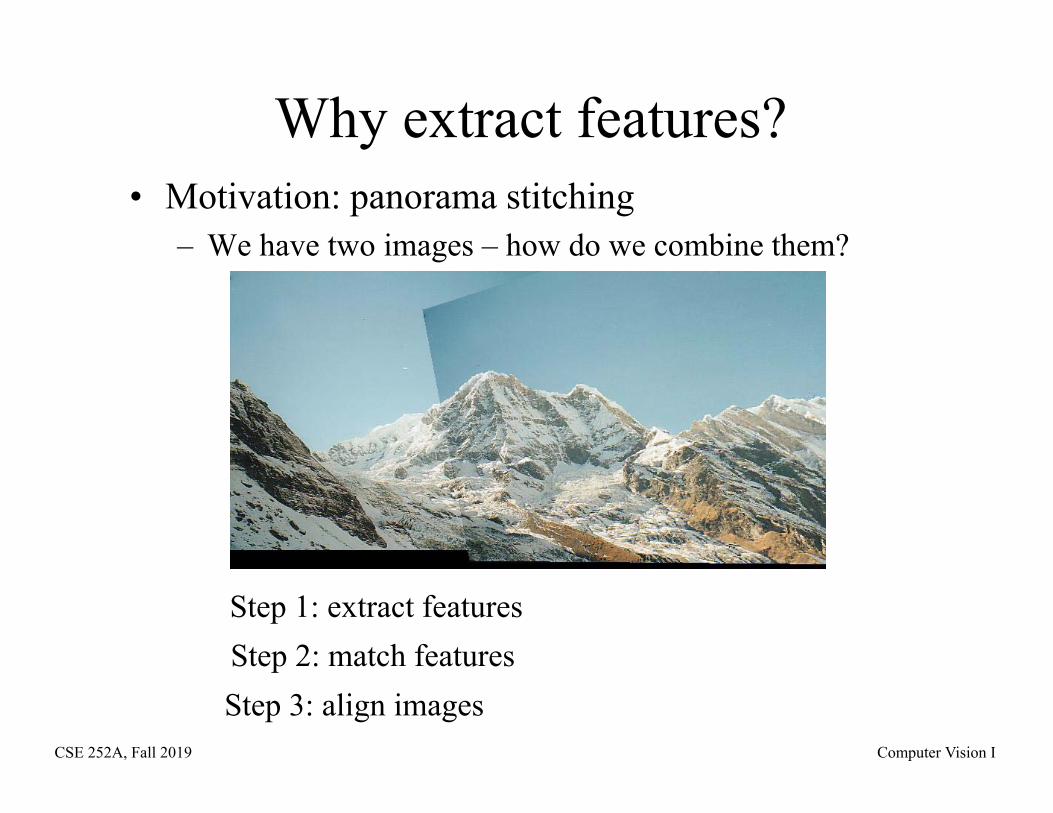
Why extract features?• Motivation: panorama stitching
– We have two images – how do we combine them?
CSE 252A, Fall 2019 Computer Vision I
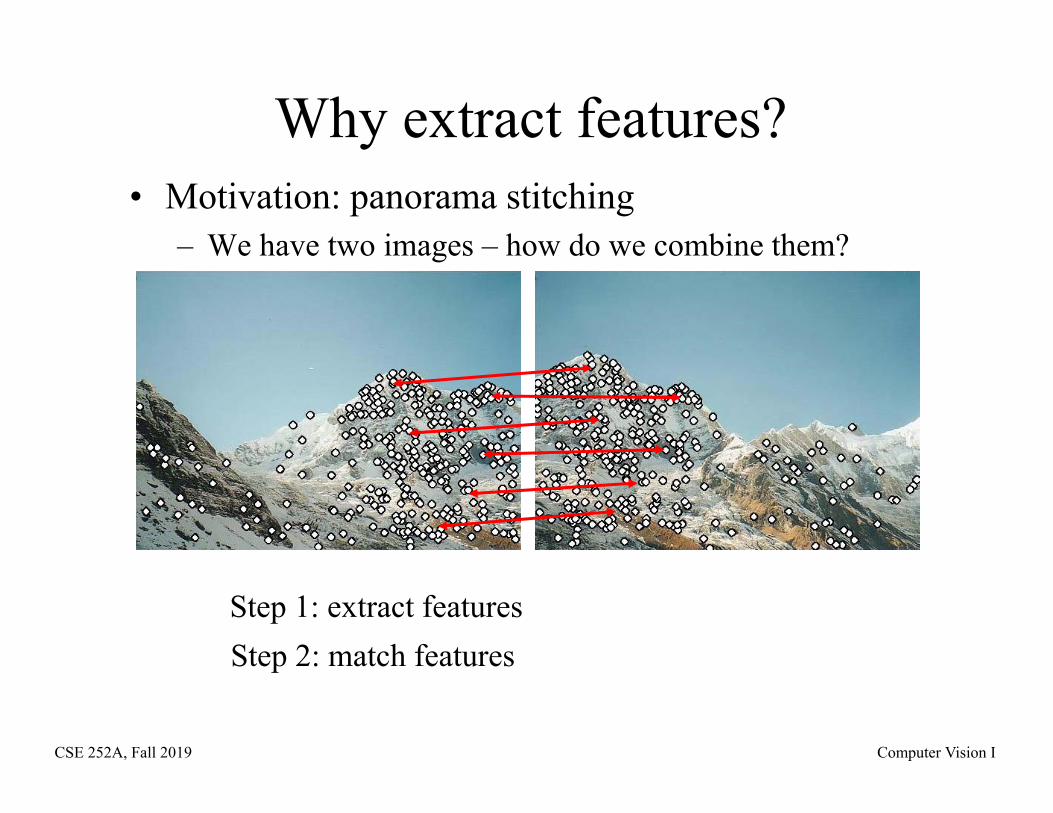
Why extract features?• Motivation: panorama stitching
– We have two images – how do we combine them?
Step 1: extract featuresStep 2: match features
CSE 252A, Fall 2019 Computer Vision I
Why extract features?• Motivation: panorama stitching
– We have two images – how do we combine them?
Step 1: extract featuresStep 2: match featuresStep 3: align images
CSE 252A, Fall 2019 Computer Vision I
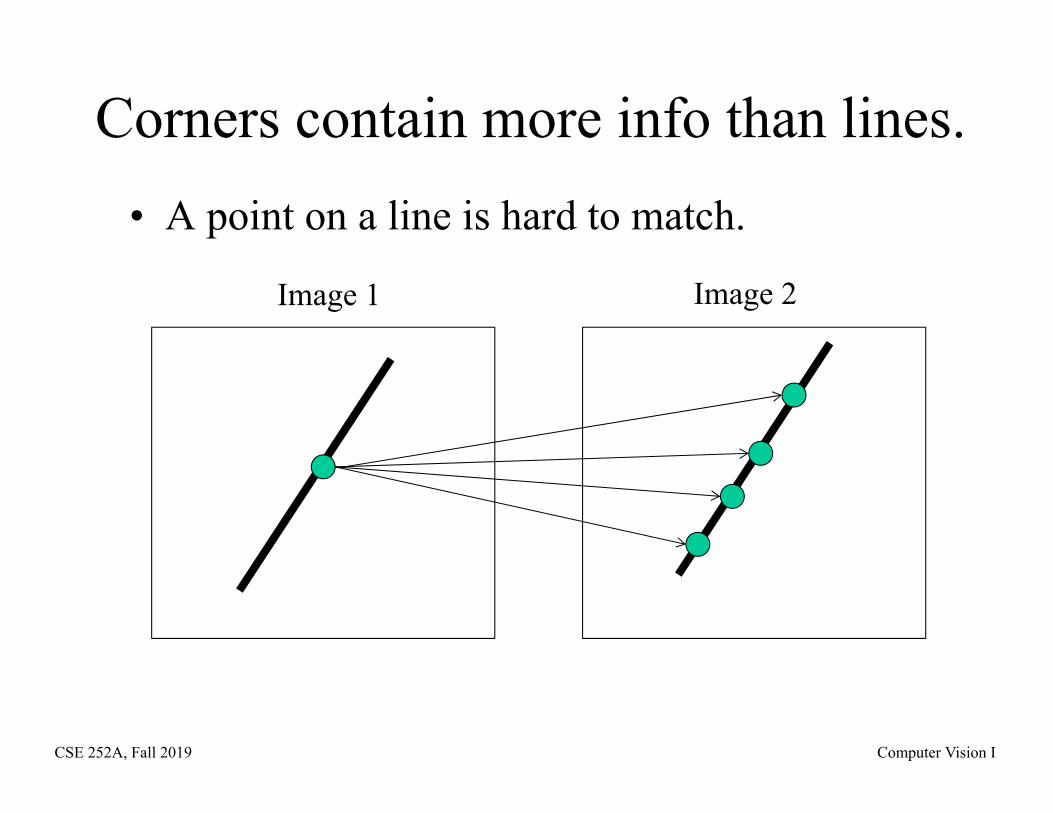
Corners contain more info than lines.• A point on a line is hard to match.
Image 1 Image 2
CSE 252A, Fall 2019 Computer Vision I
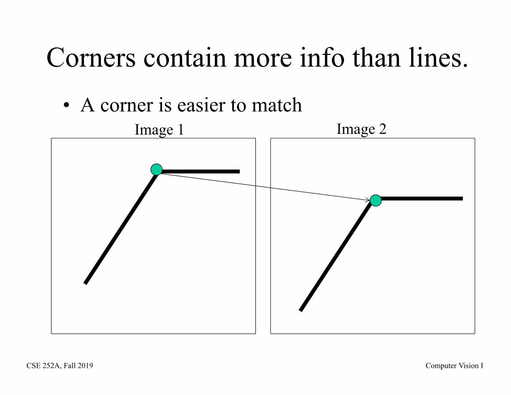
Corners contain more info than lines.• A corner is easier to match
Image 1 Image 2
CSE 252A, Fall 2019 Computer Vision I
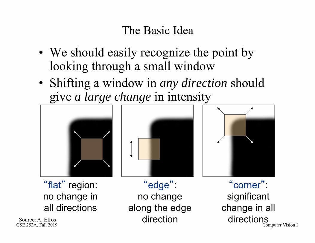
The Basic Idea
• We should easily recognize the point by looking through a small window
• Shifting a window in any direction should give a large change in intensity
“edge”:no change
along the edge direction
“corner”:significant
change in all directions
“flat” region:no change in all directions
Source: A. Efros
CSE 252A, Fall 2019 Computer Vision I
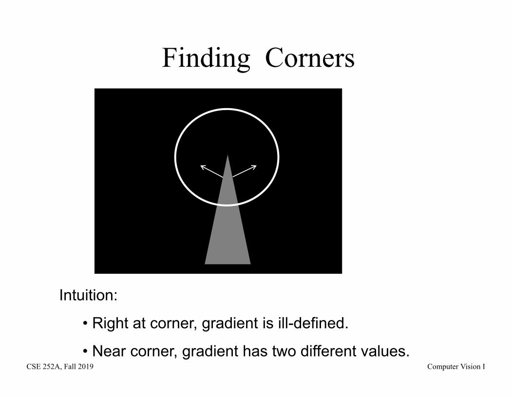
Finding Corners
Intuition:
• Right at corner, gradient is ill-defined.
• Near corner, gradient has two different values.
CSE 252A, Fall 2019 Computer Vision I
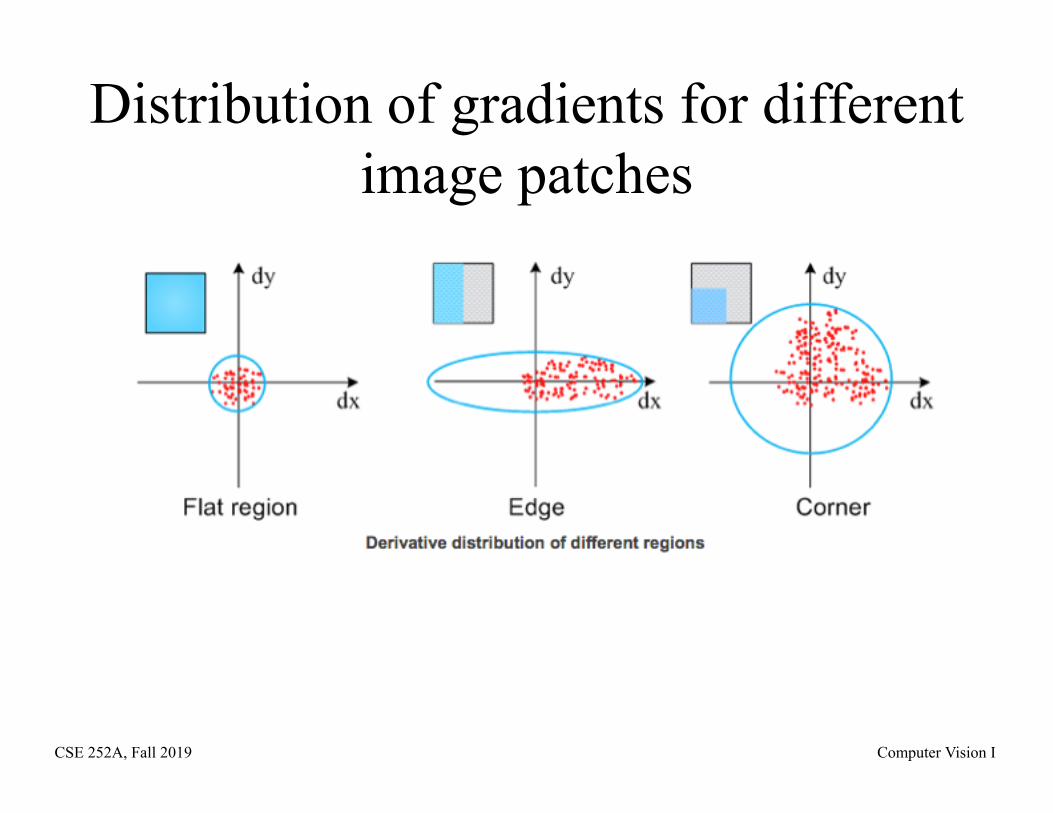
Distribution of gradients for different image patches
CSE 252A, Fall 2019 Computer Vision I
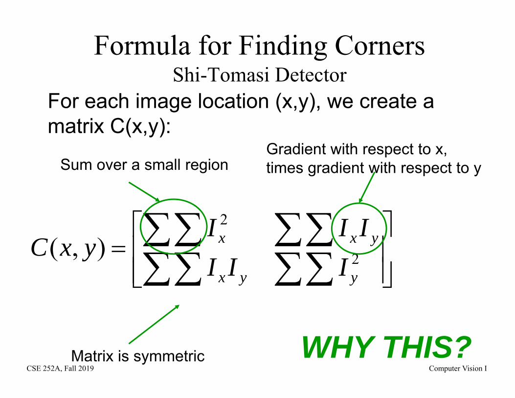
Formula for Finding CornersShi-Tomasi Detector
2
2
),(yyx
yxx
IIIIII
yxC
For each image location (x,y), we create a matrix C(x,y):
Sum over a small regionGradient with respect to x, times gradient with respect to y
Matrix is symmetric WHY THIS?
CSE 252A, Fall 2019 Computer Vision I
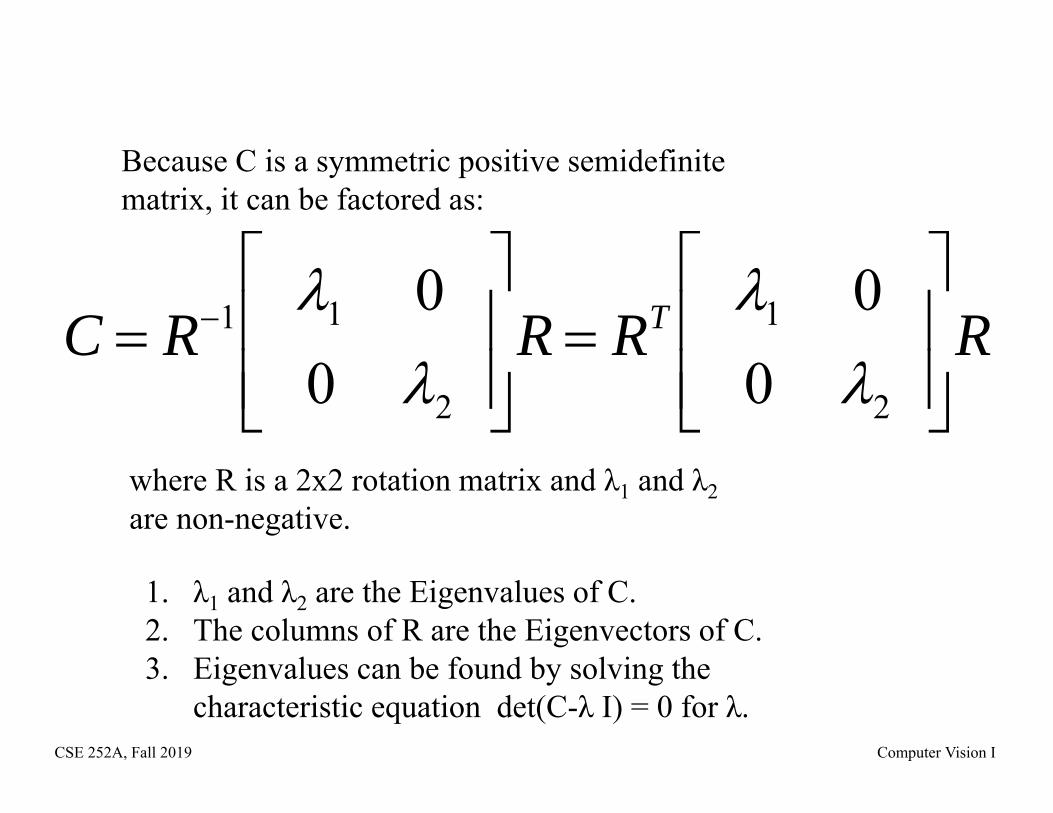
Because C is a symmetric positive semidefinite matrix, it can be factored as:
C R1 1 00 2
R RT 1 0
0 2
R
where R is a 2x2 rotation matrix and λ1 and λ2 are non-negative.
1. λ1 and λ2 are the Eigenvalues of C. 2. The columns of R are the Eigenvectors of C.3. Eigenvalues can be found by solving the
characteristic equation det(C-λ I) = 0 for λ.
CSE 252A, Fall 2019 Computer Vision I
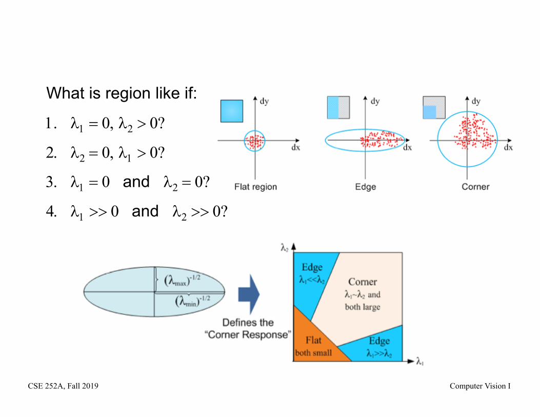
What is region like if:
and
and
CSE 252A, Fall 2019 Computer Vision I
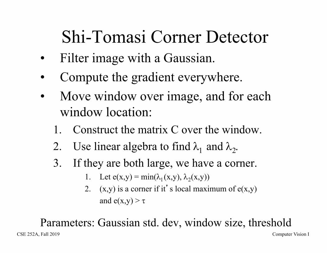
Shi-Tomasi Corner Detector• Filter image with a Gaussian.• Compute the gradient everywhere.• Move window over image, and for each
window location:1. Construct the matrix C over the window.2. Use linear algebra to find and 3. If they are both large, we have a corner.
1. Let e(x,y) = min((x,y), (x,y)2. (x,y) is a corner if it’s local maximum of e(x,y)
and e(x,y) >
Parameters: Gaussian std. dev, window size, threshold
CSE 252A, Fall 2019 Computer Vision I
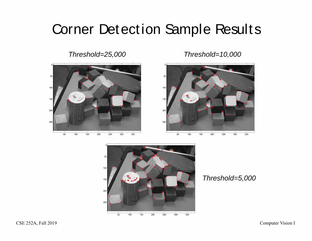
Corner Detection Sample Results
Threshold=25,000 Threshold=10,000
Threshold=5,000
CSE 252A, Fall 2019 Computer Vision I
Next Lecture• Early vision: multiple images
– Stereo• Reading:
– Chapter 7: Stereopsis


![EDGE DETECTION AND SKELETONIZATION USING QUANTIZED LOCALIZED PHASE · 2009-08-07 · edge and corner detection and segmentation and in comple-menting magnitude information [5],[6]](https://img.pdfslide.us/doc/110x75/5ec99bd002f2c14ba77679b8/edge-detection-and-skeletonization-using-quantized-localized-phase-2009-08-07.jpg)