Embed Size (px)
Citation preview
Concentration inequalities and martingale
inequalities — a survey
Fan Chung ∗† Linyuan Lu ‡†
May 28, 2006
Abstract
We examine a number of generalized and extended versions of concen-tration inequalities and martingale inequalities. These inequalities are ef-fective for analyzing processes with quite general conditions as illustratedin an example for an infinite Polya process and webgraphs.
1 Introduction
One of the main tools in probabilistic analysis is the concentration inequalities.Basically, the concentration inequalities are meant to give a sharp predictionof the actual value of a random variable by bounding the error term (from theexpected value) with an associated probability. The classical concentration in-equalities such as those for the binomial distribution have the best possible errorestimates with exponentially small probabilistic bounds. Such concentration in-equalities usually require certain independence assumptions (i.e., the randomvariable can be decomposed as a sum of independent random variables).
When the independence assumptions do not hold, it is still desirable to havesimilar, albeit slightly weaker, inequalities at our disposal. One approach isthe martingale method. If the random variable and the associated probabilityspace can be organized into a chain of events with modified probability spacesand if the incremental changes of the value of the event is “small”, then themartingale inequalities provide very good error estimates. The reader is referredto numerous textbooks [5, 17, 20] on this subject.
In the past few years, there has been a great deal of research in analyzinggeneral random graph models for realistic massive graphs which have unevendegree distribution such as the power law [1, 2, 3, 4, 6]. The usual concentrationinequalities and martingale inequalities have often been found to be inadequateand in many cases not feasible. The reasons are multi-fold: Due to unevendegree distribution, the error bound of those very large degrees offset the delicate
∗University of California, San Diego, [email protected]†Research supported in part by NSF Grants DMS 0100472 and ITR 0205061‡University of South Carolina, [email protected]
1
analysis in the sparse part of the graph. For the setup of the martingales, auniform upper bound for the incremental changes are often too poor to be ofany use. Furthermore, the graph is dynamically evolving and therefore theprobability space is changing at each tick of the time.
In spite of these difficulties, it is highly desirable to extend the classical con-centration inequalities and martingale inequalities so that rigorous analysis forrandom graphs with general degree distributions can be carried out. Indeed, inthe course of studying general random graphs, a number of variations and gen-eralizations of concentration inequalities and martingale inequalities have beenscattered around. It is the goal of this survey to put together these extensionsand generalizations to present a more complete picture. We will examine andcompare these inequalities and complete proofs will be given. Needless to saythat this survey is far from complete since all the work is quite recent and theselection is heavily influenced by our personal learning experience on this topic.Indeed, many of these inequalities have been included in our previous papers[9, 10, 11, 12].
In addition to numerous variations of the inequalities, we also include anexample of an application on a generalization of Polya’s urn problem. Dueto the fundamental nature of these concentration inequalities and martingaleinequalities, they may be useful for many other problems as well.
This paper is organized as follows:
1. Introduction — overview, recent developments and summary.
2. Binomial distribution and its asymptotic behavior — the normalized bi-nomial distribution and Poisson distribution,
3. General Chernoff inequalities — sums of independent random variables infive different concentration inequalities.
4. More concentration inequalities — five more variations of the concentra-tion inequalities.
5. Martingales and Azuma’s inequality — basics for martingales and proofsfor Azuma’s inequality.
6. General martingale inequalities — four general versions of martingale in-equalities with proofs.
7. Supermartingales and submartingales — modifying the definitions formartingale and still preserving the effectiveness of the martingale inequal-ities.
8. The decision tree and relaxed concentration inequalities — instead of theworst case incremental bound (the Lipschitz condition), only certain ‘local’conditions are required.
9. A generalized Polya’s urn problem — An application for an infinite Polyaprocess by using these general concentration and martingale inequalities.
2
For webgraphs generated by the preferential attachment scheme, the con-centration for the power law degree distribution can be derived in a similarway.
2 The binomial distribution and its asymptotic
behavior
Bernoulli trials, named after James Bernoulli, can be thought of as a sequenceof coin flips. For some fixed value p, where 0 ≤ p ≤ 1, the outcome of thecoin tossing process has probability p of getting a “head”. Let Sn denote thenumber of heads after n tosses. We can write Sn as a sum of independentrandom variables Xi as follows:
Sn = X1 + X2 + · · · + Xn
where, for each i, the random variable X satisfies
Pr(Xi = 1) = p,
Pr(Xi = 0) = 1 − p. (1)
A classical question is to determine the distribution of Sn. It is not too difficultto see that Sn has the binomial distribution B(n, p):
Pr(Sn = k) =(
n
k
)pk(1 − p)n−k, for k = 0, 1, 2, . . . , n.
The expectation and variance of B(n, p) are
E(Sn) = np, Var(Sn) = np(1 − p).
To better understand the asymptotic behavior of the binomial distribution,we compare it with the normal distribution N(α, σ), whose density function isgiven by
f(x) =1√2πσ
e−(x−α)2
2σ2 , −∞ < x < ∞
where α denotes the expectation and σ2 is the variance.The case N(0, 1) is called the standard normal distribution whose density
function is given by
f(x) =1√2π
e−x2/2, −∞ < x < ∞.
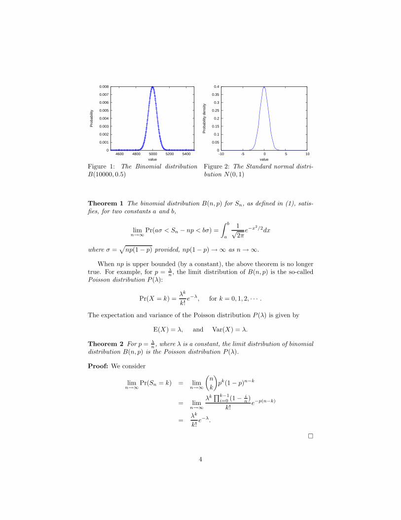
When p is a constant, the limit of the binomial distribution, after scaling,is the standard normal distribution and can be viewed as a special case of theCentral-Limit Theorem, sometimes called the DeMoivre-Laplace limit Theorem[15].
3
0
0.001
0.002
0.003
0.004
0.005
0.006
0.007
0.008
4600 4800 5000 5200 5400
Pro
babi
lity
value
0
0.05
0.1
0.15
0.2
0.25
0.3
0.35
0.4
-10 -5 0 5 10
Pro
babi
lity
dens
ity
value
Figure 1: The Binomial distributionB(10000, 0.5)
Figure 2: The Standard normal distri-bution N(0, 1)
Theorem 1 The binomial distribution B(n, p) for Sn, as defined in (1), satis-fies, for two constants a and b,
limn→∞ Pr(aσ < Sn − np < bσ) =
∫ b
a
1√2π
e−x2/2dx
where σ =√
np(1 − p) provided, np(1 − p) → ∞ as n → ∞.
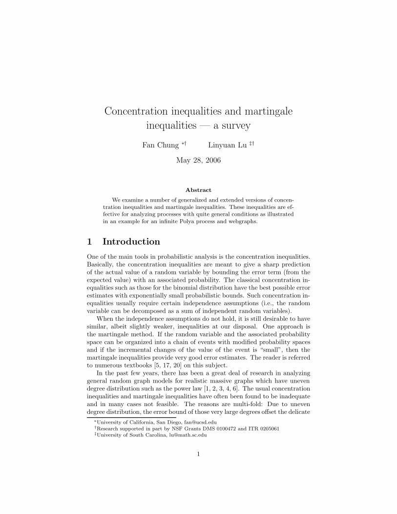
When np is upper bounded (by a constant), the above theorem is no longertrue. For example, for p = λ
n , the limit distribution of B(n, p) is the so-calledPoisson distribution P (λ):
Pr(X = k) =λk
k!e−λ, for k = 0, 1, 2, · · · .
The expectation and variance of the Poisson distribution P (λ) is given by
E(X) = λ, and Var(X) = λ.
Theorem 2 For p = λn , where λ is a constant, the limit distribution of binomial
distribution B(n, p) is the Poisson distribution P (λ).
Proof: We consider
limn→∞ Pr(Sn = k) = lim
n→∞
(n
k
)pk(1 − p)n−k
= limn→∞
λk∏k−1
i=0 (1 − in )
k!e−p(n−k)
=λk
k!e−λ.
4
0
0.05
0.1
0.15
0.2
0.25
0 5 10 15 20
Pro
babi
lity
value
0
0.05
0.1
0.15
0.2
0.25
0 5 10 15 20
Pro
babi
lity
value
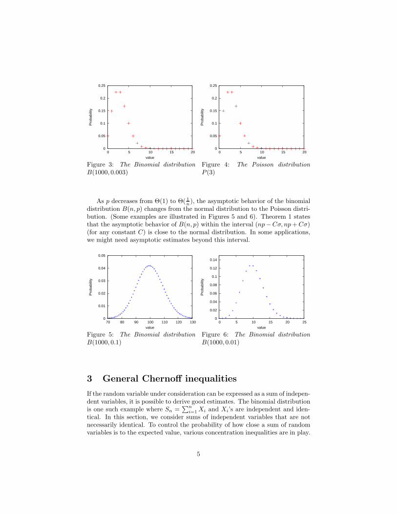
Figure 3: The Binomial distributionB(1000, 0.003)
Figure 4: The Poisson distributionP (3)
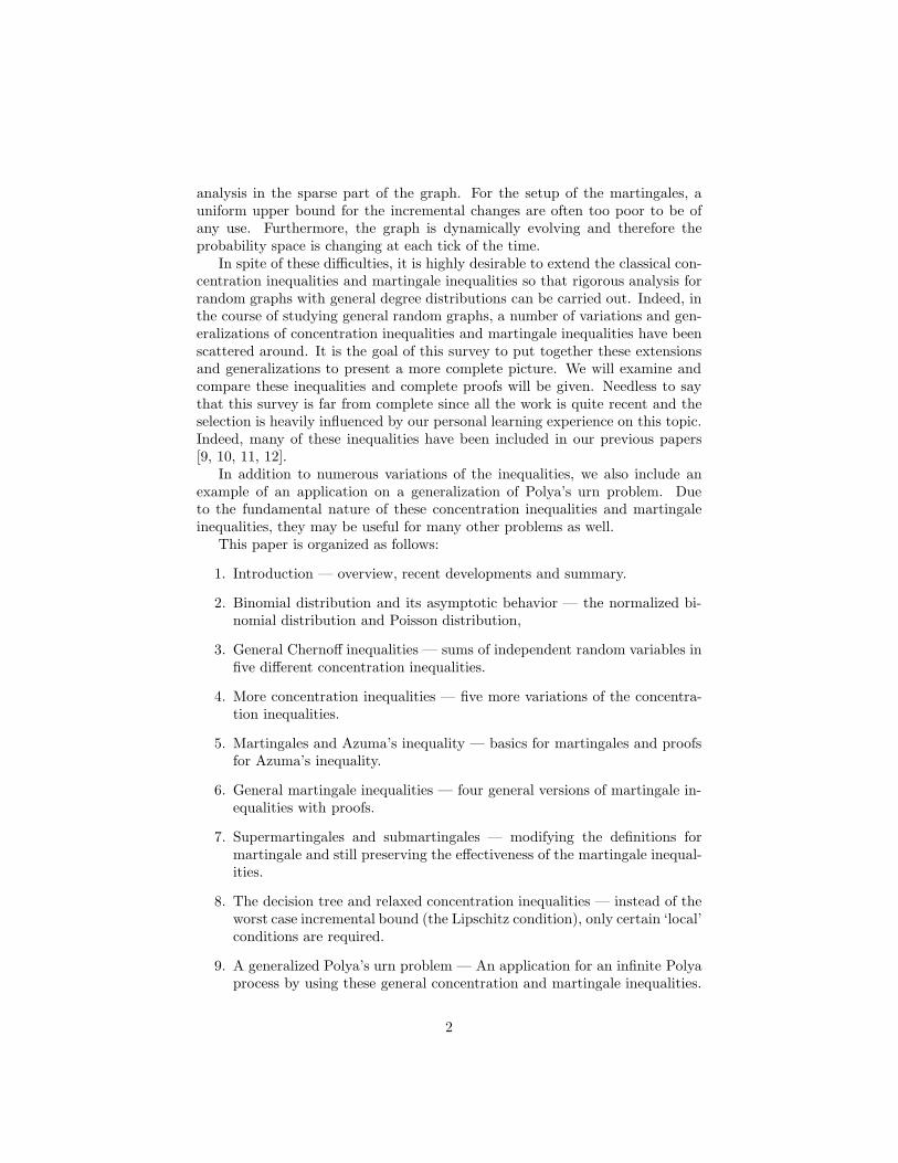
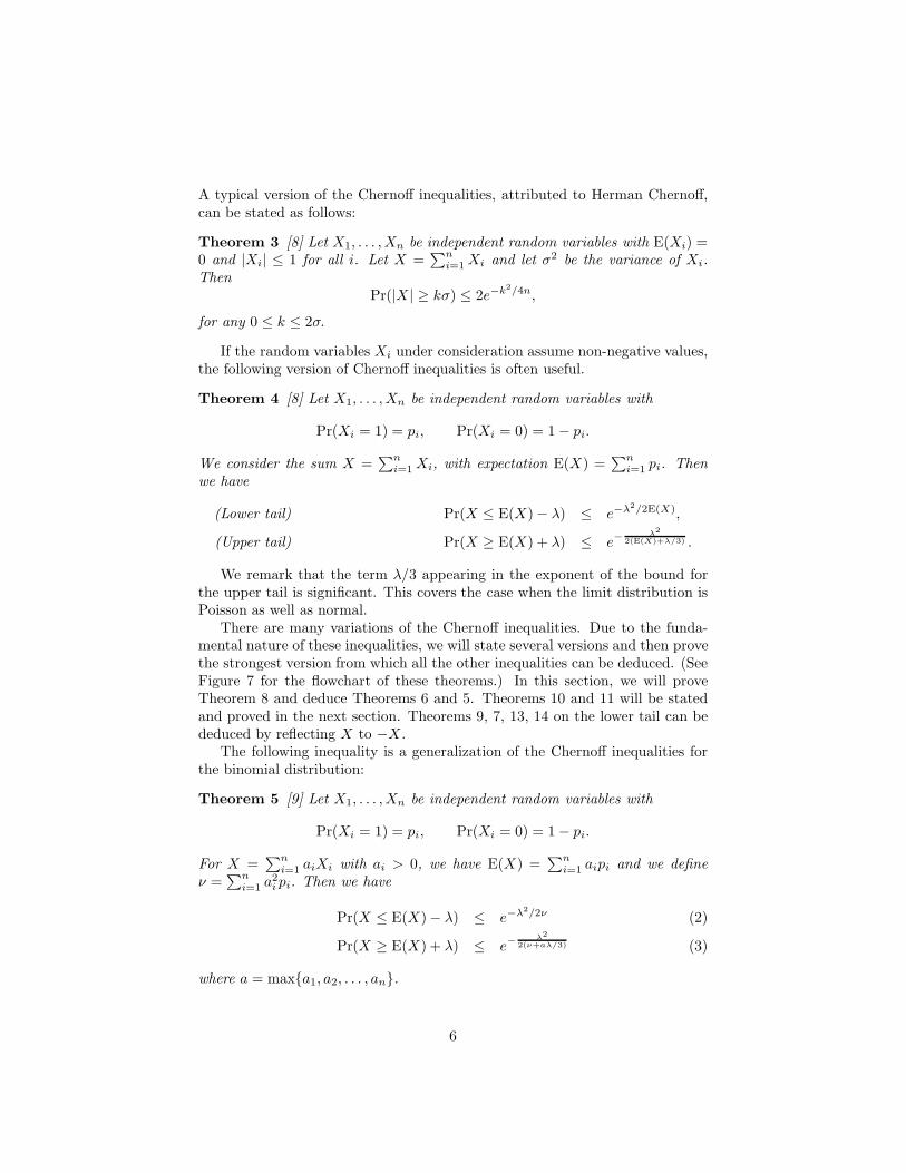
As p decreases from Θ(1) to Θ( 1n ), the asymptotic behavior of the binomial
distribution B(n, p) changes from the normal distribution to the Poisson distri-bution. (Some examples are illustrated in Figures 5 and 6). Theorem 1 statesthat the asymptotic behavior of B(n, p) within the interval (np−Cσ, np + Cσ)(for any constant C) is close to the normal distribution. In some applications,we might need asymptotic estimates beyond this interval.
0
0.01
0.02
0.03
0.04
0.05
70 80 90 100 110 120 130
Pro
babi
lity
value
0
0.02
0.04
0.06
0.08
0.1
0.12
0.14
0 5 10 15 20 25
Pro
babi
lity
value
Figure 5: The Binomial distributionB(1000, 0.1)
Figure 6: The Binomial distributionB(1000, 0.01)
3 General Chernoff inequalities
If the random variable under consideration can be expressed as a sum of indepen-dent variables, it is possible to derive good estimates. The binomial distributionis one such example where Sn =
∑ni=1 Xi and Xi’s are independent and iden-
tical. In this section, we consider sums of independent variables that are notnecessarily identical. To control the probability of how close a sum of randomvariables is to the expected value, various concentration inequalities are in play.
5
A typical version of the Chernoff inequalities, attributed to Herman Chernoff,can be stated as follows:
Theorem 3 [8] Let X1, . . . , Xn be independent random variables with E(Xi) =0 and |Xi| ≤ 1 for all i. Let X =
∑ni=1 Xi and let σ2 be the variance of Xi.
ThenPr(|X | ≥ kσ) ≤ 2e−k2/4n,
for any 0 ≤ k ≤ 2σ.
If the random variables Xi under consideration assume non-negative values,the following version of Chernoff inequalities is often useful.
Theorem 4 [8] Let X1, . . . , Xn be independent random variables with
Pr(Xi = 1) = pi, Pr(Xi = 0) = 1 − pi.
We consider the sum X =∑n
i=1 Xi, with expectation E(X) =∑n
i=1 pi. Thenwe have
(Lower tail) Pr(X ≤ E(X) − λ) ≤ e−λ2/2E(X),
(Upper tail) Pr(X ≥ E(X) + λ) ≤ e−λ2
2(E(X)+λ/3) .
We remark that the term λ/3 appearing in the exponent of the bound forthe upper tail is significant. This covers the case when the limit distribution isPoisson as well as normal.
There are many variations of the Chernoff inequalities. Due to the funda-mental nature of these inequalities, we will state several versions and then provethe strongest version from which all the other inequalities can be deduced. (SeeFigure 7 for the flowchart of these theorems.) In this section, we will proveTheorem 8 and deduce Theorems 6 and 5. Theorems 10 and 11 will be statedand proved in the next section. Theorems 9, 7, 13, 14 on the lower tail can bededuced by reflecting X to −X .
The following inequality is a generalization of the Chernoff inequalities forthe binomial distribution:
Theorem 5 [9] Let X1, . . . , Xn be independent random variables with
Pr(Xi = 1) = pi, Pr(Xi = 0) = 1 − pi.
For X =∑n
i=1 aiXi with ai > 0, we have E(X) =∑n
i=1 aipi and we defineν =
∑ni=1 a2
i pi. Then we have
Pr(X ≤ E(X) − λ) ≤ e−λ2/2ν (2)
Pr(X ≥ E(X) + λ) ≤ e−λ2
2(ν+aλ/3) (3)
where a = maxa1, a2, . . . , an.
6
Theorem 8 Theorem 9
Theorem 6 Theorem 7
Theorem 5
Theorem 4
Theorem 10 Theorem 13 Theorem 14Theorem 11
Upper tails Lower tails
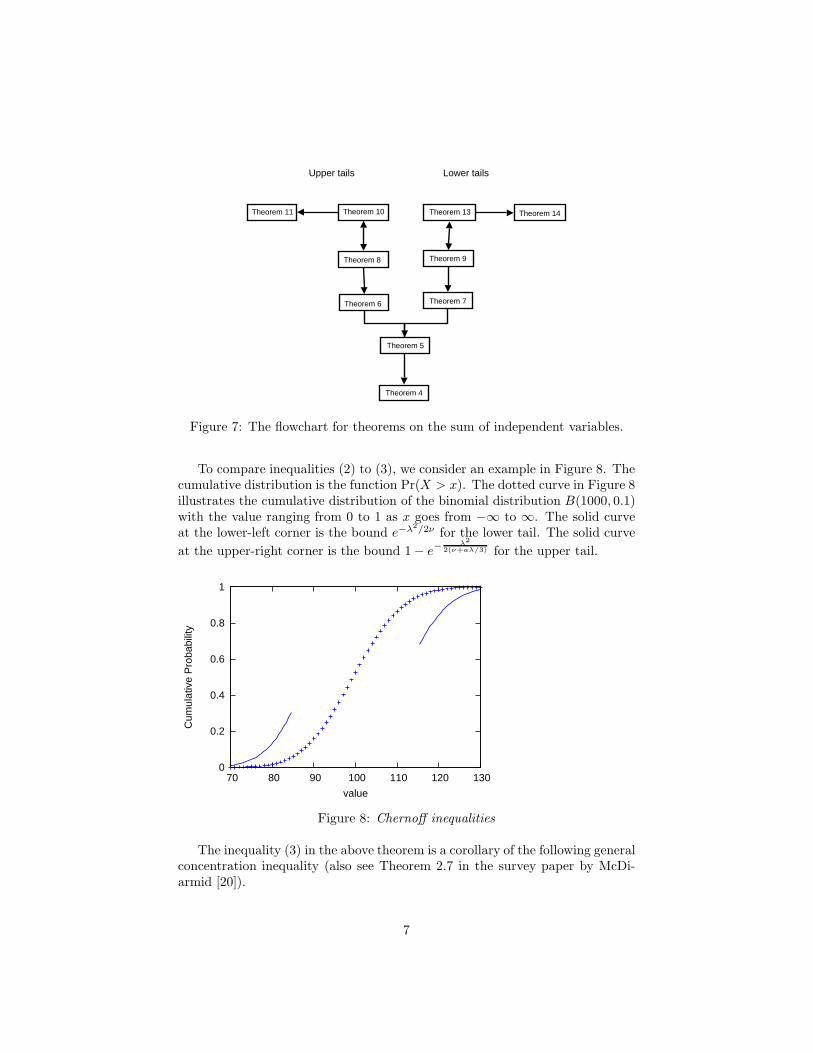
Figure 7: The flowchart for theorems on the sum of independent variables.
To compare inequalities (2) to (3), we consider an example in Figure 8. Thecumulative distribution is the function Pr(X > x). The dotted curve in Figure 8illustrates the cumulative distribution of the binomial distribution B(1000, 0.1)with the value ranging from 0 to 1 as x goes from −∞ to ∞. The solid curveat the lower-left corner is the bound e−λ2/2ν for the lower tail. The solid curveat the upper-right corner is the bound 1 − e−
λ22(ν+aλ/3) for the upper tail.
0
0.2
0.4
0.6
0.8
1
70 80 90 100 110 120 130
Cum
ulat
ive
Pro
babi
lity
value
Figure 8: Chernoff inequalities
The inequality (3) in the above theorem is a corollary of the following generalconcentration inequality (also see Theorem 2.7 in the survey paper by McDi-armid [20]).
7
Theorem 6 [20] Let Xi (1 ≤ i ≤ n) be independent random variables satisfyingXi ≤ E(Xi) + M , for 1 ≤ i ≤ n. We consider the sum X =
∑ni=1 Xi with
expectation E(X) =∑n
i=1 E(Xi) and variance Var(X) =∑n
i=1 Var(Xi). Thenwe have
Pr(X ≥ E(X) + λ) ≤ e−λ2
2(Var(X)+Mλ/3) .
In the other direction, we have the following inequality.
Theorem 7 If X1, X2, . . . , Xn are non-negative independent random variables,we have the following bounds for the sum X =
∑ni=1 Xi:
Pr(X ≤ E(X) − λ) ≤ e− λ2
2Pn
i=1 E(X2i) .
A strengthened version of the above theorem is as follows:
Theorem 8 Suppose Xi are independent random variables satisfying Xi ≤ M ,for 1 ≤ i ≤ n. Let X =
∑ni=1 Xi and ‖X‖ =
√∑ni=1 E(X2
i ). Then we have
Pr(X ≥ E(X) + λ) ≤ e− λ2
2(‖X‖2+Mλ/3) .
Replacing X by −X in the proof of Theorem 8, we have the following theoremfor the lower tail.
Theorem 9 Let Xi be independent random variables satisfying Xi ≥ −M , for1 ≤ i ≤ n. Let X =
∑ni=1 Xi and ‖X‖ =
√∑ni=1 E(X2
i ). Then we have
Pr(X ≤ E(X) − λ) ≤ e− λ2
2(‖X‖2+Mλ/3) .
Before we give the proof of Theorems 8, we will first show the implicationsof Theorems 8 and 9. Namely, we will show that the other concentration in-equalities can be derived from Theorems 8 and 9.
Fact: Theorem 8 =⇒ Theorem 6:
Proof: Let X ′i = Xi − E(Xi) and X ′ =
∑ni=1 X ′
i = X − E(X). We have
X ′i ≤ M for 1 ≤ i ≤ n.
We also have
‖X ′‖2 =n∑
i=1
E(X ′2i )
=n∑
i=1
Var(Xi)
= Var(X).
8
Applying Theorem 8, we get
Pr(X ≥ E(X) + λ) = Pr(X ′ ≥ λ)
≤ e− λ2
2(‖X′‖2+Mλ/3)
≤ e− λ2
2(Var(X)+Mλ/3) .
Fact: Theorem 9 =⇒ Theorem 7The proof is straightforward by choosing M = 0.
Fact: Theorem 6 and 7 =⇒ Theorem 5Proof: We define Yi = aiXi. Note that
‖X‖2 =n∑
i=1
E(Y 2i ) =
n∑i=1
a2i pi = ν.
Equation (2) follows from Theorem 7 since Yi’s are non-negatives.For the other direction, we have
Yi ≤ ai ≤ a ≤ E(Yi) + a.
Equation (3) follows from Theorem 6.
Fact: Theorem 8 and Theorem 9 =⇒ Theorem 3The proof is by choosing Y = X − E(X), M = 1 and applying Theorems 8 andTheorem 9 to Y .
Fact: Theorem 5 =⇒ Theorem 4The proof follows by choosing a1 = a2 = · · · = an = 1.
Finally, we give the complete proof of Theorem 8 and thus finish the proofsfor all the above theorems on Chernoff inequalities.Proof of Theorem 8: We consider
E(etX) = E(etP
i Xi) =n∏
i=1
E(etXi)
since the Xi’s are independent.We define g(y) = 2
∑∞k=2
yk−2
k! = 2(ey−1−y)y2 , and use the following facts about
g:
• g(0) = 1.
• g(y) ≤ 1, for y < 0.
• g(y) is monotone increasing, for y ≥ 0.
9
• For y < 3, we have
g(y) = 2∞∑
k=2
yk−2
k!≤
∞∑k=2
yk−2
3k−2=
11 − y/3
since k! ≥ 2 · 3k−2.
Then we have, for k ≥ 2,
E(etX) =n∏
i=1
E(etXi)
=n∏
i=1
E(∞∑
k=0
tkXki
k!)
=n∏
i=1
E(1 + tE(Xi) +12t2X2
i g(tXi))
≤n∏
i=1
(1 + tE(Xi) +12t2E(X2
i )g(tM))
≤n∏
i=1
etE(Xi)+12 t2E(X2
i )g(tM)
= etE(X)+ 12 t2g(tM)
Pni=1 E(X2
i )
= etE(X)+ 12 t2g(tM)‖X‖2
.
Hence, for t satisfying tM < 3, we have
Pr(X ≥ E(X) + λ) = Pr(etX ≥ etE(X)+tλ)≤ e−tE(X)−tλE(etX)
≤ e−tλ+ 12 t2g(tM)‖X‖2
≤ e−tλ+ 12 t2‖X‖2 1
1−tM/3 .
To minimize the above expression, we choose t = λ‖X‖2+Mλ/3 . Therefore, tM <
3 and we have
Pr(X ≥ E(X) + λ) ≤ e−tλ+ 12 t2‖X‖2 1
1−tM/3
= e− λ2
2(‖X‖2+Mλ/3) .
The proof is complete.
4 More concentration inequalities
Here we state several variations and extensions of the concentration inequalitiesin Theorem 8. We first consider the upper tail.
10
Theorem 10 Let Xi denote independent random variables satisfying Xi ≤E(Xi) + ai + M , for 1 ≤ i ≤ n. For, X =
∑ni=1 Xi, we have
Pr(X ≥ E(X) + λ) ≤ e− λ2
2(Var(X)+Pn
i=1 a2i+Mλ/3) .
Proof: Let X ′i = Xi − E(Xi) − ai and X ′ =
∑ni=1 X ′
i. We have
X ′i ≤ M for 1 ≤ i ≤ n.
X ′ − E(X ′) =n∑
i=1
(X ′i − E(X ′
i))
=n∑
i=1
(X ′i + ai)
=n∑
i=1
(Xi − E(Xi))
= X − E(X).
Thus,
‖X ′‖2 =n∑
i=1
E(X ′2i )
=n∑
i=1
E((Xi − E(Xi) − ai)2)
=n∑
i=1
E((Xi − E(Xi))2 + a2i
= Var(X) +n∑
i=1
a2i .
By applying Theorem 8, the proof is finished.
Theorem 11 Suppose Xi are independent random variables satisfying Xi ≤E(Xi) + Mi, for 0 ≤ i ≤ n. We order the Xi’s so that the Mi are in increasingorder. Let X =
∑ni=1 Xi. Then for any 1 ≤ k ≤ n, we have
Pr(X ≥ E(X) + λ) ≤ e− λ2
2(Var(X)+Pn
i=k(Mi−Mk)2+Mkλ/3) .
Proof: For fixed k, we choose M = Mk and
ai =
0 if 1 ≤ i ≤ k,Mi − Mk if k ≤ i ≤ n.
We haveXi − E(Xi) ≤ Mi ≤ ai + Mk for 1 ≤ k ≤ n,
11
n∑i=1
a2i =
n∑i=k
(Mi − Mk)2.
Using Theorem 10, we have
Pr(Xi ≥ E(X) + λ) ≤ e− λ2
2(Var(X)+Pn
i=k(Mi−Mk)2+Mkλ/3) .
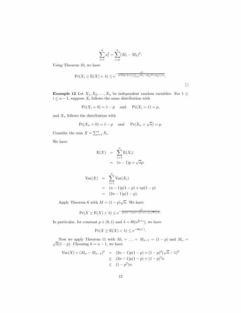
Example 12 Let X1, X2, . . . , Xn be independent random variables. For 1 ≤i ≤ n − 1, suppose Xi follows the same distribution with
Pr(Xi = 0) = 1 − p and Pr(Xi = 1) = p,
and Xn follows the distribution with
Pr(Xn = 0) = 1 − p and Pr(Xn =√
n) = p.
Consider the sum X =∑n
i=1 Xi.
We have
E(X) =n∑
i=1
E(Xi)
= (n − 1)p +√
np.
Var(X) =n∑
i=1
Var(Xi)
= (n − 1)p(1 − p) + np(1 − p)= (2n − 1)p(1 − p).
Apply Theorem 6 with M = (1 − p)√
n. We have
Pr(X ≥ E(X) + λ) ≤ e− λ2
2((2n−1)p(1−p)+(1−p)√
nλ/3) .
In particular, for constant p ∈ (0, 1) and λ = Θ(n12 +ε), we have
Pr(X ≥ E(X) + λ) ≤ e−Θ(nε).
Now we apply Theorem 11 with M1 = . . . = Mn−1 = (1 − p) and Mn =√n(1 − p). Choosing k = n − 1, we have
Var(X) + (Mn − Mn−1)2 = (2n − 1)p(1 − p) + (1 − p)2(√
n − 1)2
≤ (2n − 1)p(1 − p) + (1 − p)2n≤ (1 − p2)n.
12
Thus,
Pr(Xi ≥ E(X) + λ) ≤ e− λ2
2((1−p2)n+(1−p)2λ/3) .
For constant p ∈ (0, 1) and λ = Θ(n12+ε), we have
Pr(X ≥ E(X) + λ) ≤ e−Θ(n2ε).
From the above examples, we note that Theorem 11 gives a significantlybetter bound than that in Theorem 6 if the random variables Xi have verydifferent upper bounds.
For completeness, we also list the corresponding theorems for the lower tails.(These can be derived by replacing X by −X .)
Theorem 13 Let Xi denote independent random variables satisfying Xi ≥E(Xi) − ai − M , for 0 ≤ i ≤ n. For X =
∑ni=1 Xi, we have
Pr(X ≤ E(X) − λ) ≤ e− λ2
2(Var(X)+Pn
i=1 a2i+Mλ/3) .
Theorem 14 Let Xi denote independent random variables satisfying Xi ≥E(Xi) − Mi, for 0 ≤ i ≤ n. We order the Xi’s so that the Mi are in increasingorder. Let X =
∑ni=1 Xi. Then for any 1 ≤ k ≤ n, we have
Pr(X ≤ E(X) − λ) ≤ e− λ2
2(Var(X)+Pn
i=k(Mi−Mk)2+Mkλ/3) .
Continuing the above example, we choose M1 = M2 = . . . = Mn−1 = p, andMn =
√np. We choose k = n − 1, so we have
Var(X) + (Mn − Mn−1)2 = (2n − 1)p(1 − p) + p2(√
n − 1)2
≤ (2n − 1)p(1 − p) + p2n
≤ p(2 − p)n.
Using Theorem 14, we have
Pr(X ≤ E(X) − λ) ≤ e− λ2
2(p(2−p)n+p2λ/3) .
For a constant p ∈ (0, 1) and λ = Θ(n12 +ε), we have
Pr(X ≤ E(X) − λ) ≤ e−Θ(n2ε).
5 Martingales and Azuma’s inequality
A martingale is a sequence of random variables X0, X1, . . . with finite meanssuch that the conditional expectation of Xn+1 given X0, X1, . . . , Xn is equal toXn.
The above definition is given in the classical book of Feller [15], p. 210.However, the conditional expectation depends on the random variables under
13
consideration and can be difficult to deal with in various cases. In this surveywe will use the following definition which is concise and basically equivalent forthe finite cases.
Suppose that Ω is a probability space with a probability distribution p. LetF denote a σ-field on Ω. (A σ-field on Ω is a collection of subsets of Ω whichcontains ∅ and Ω, and is closed under unions, intersections, and complementa-tion.) In a σ-field F of Ω, the smallest set in F containing an element x is theintersection of all sets in F containing x. A function f : Ω → R is said to beF -measurable if f(x) = f(y) for any y in the smallest set containing x. (Formore terminology on martingales, the reader is referred to [17].)
If f : Ω → R is a function, we define the expectation E(f) = E(f(x) | x ∈ Ω)by
E(f) = E(f(x) | x ∈ Ω) :=∑x∈Ω
f(x)p(x).
If F is a σ-field on Ω, we define the conditional expectation E(f | F) : Ω → R
by the formula
E(f | F)(x) :=1∑
y∈F(x) p(y)
∑y∈F(x)
f(y)p(y)
where F(x) is the smallest element of F which contains x.A filter F is an increasing chain of σ-subfields
0, Ω = F0 ⊂ F1 ⊂ · · · ⊂ Fn = F .
A martingale (obtained from) X is associated with a filter F and a sequence ofrandom variables X0, X1, . . . , Xn satisfying Xi = E(X | Fi) and, in particular,X0 = E(X) and Xn = X .
Example 15 For given independent random variables Y1, Y2, . . . , Yn, we candefine a martingale X = Y1 + Y2 + · · · + Yn as follows. Let Fi be the σ-fieldgenerated by Y1, . . . , Yi. (In other words, Fi is the minimum σ-field so thatY1, . . . , Yi are Fi-measurable.) We have a natural filter F:
0, Ω = F0 ⊂ F1 ⊂ · · · ⊂ Fn = F .
Let Xi =∑i
j=1 Yj +∑n
j=i+1 E(Yj). Then, X0, X1, X2, . . . , Xn forms a martin-gale corresponding to the filter F.
For c = (c1, c2, . . . , cn) a vector with positive entries, the martingale X issaid to be c-Lipschitz if
|Xi − Xi−1| ≤ ci (4)
for i = 1, 2, . . . , n. A powerful tool for controlling martingales is the following:
14
Theorem 16 (Azuma’s inequality) If a martingale X is c-Lipschitz, then
Pr(|X − E(X)| ≥ λ) ≤ 2e− λ2
2Pn
i=1 c2i , (5)
where c = (c1, . . . , cn).
Theorem 17 Let X1, X2, . . . , Xn be independent random variables satisfying
|Xi − E(Xi)| ≤ ci for 1 ≤ i ≤ n.
Then we have the following bound for the sum X =∑n
i=1 Xi.
Pr(|X − E(X)| ≥ λ) ≤ 2e− λ2
2Pn
i=1 c2i .
Proof of Azuma’s inequality: For a fixed t, we consider the convex functionf(x) = etx. For any |x| ≤ c, f(x) is below the line segment from (−c, f(−c)) to(c, f(c)). In other words, we have
etx ≤ 12c
(etc − e−tc)x +12
(etc + e−tc).
Therefore, we can write
E(et(Xi−Xi−1)|Fi−1) ≤ E(1
2ci(etci − e−tci)(Xi − Xi−1) +
12
(etci + e−tci)|Fi−1)
=12
(etci + e−tci)
≤ et2c2i /2.
Here we apply the conditions E(Xi − Xi−1|Fi−1) = 0 and |Xi − Xi−1| ≤ ci.Hence,
E(etXi |Fi−1) ≤ et2c2i /2etXi−1 .
Inductively, we have
E(etX) = E(E(etXn |Fn−1))
≤ et2c2n/2E(etXn−1)
≤ · · ·
≤n∏
i=1
et2c2i /2E(etX0)
= e12 t2Pn
i=1 c2i etE(X).
Therefore,
Pr(X ≥ E(X) + λ) = Pr(et(X−E(X)) ≥ etλ)≤ e−tλE(et(X−E(X)))
≤ e−tλe12 t2Pn
i=1 c2i
= e−tλ+ 12 t2Pn
i=1 c2i .
15
We choose t = λPni=1 c2
i(in order to minimize the above expression). We have
Pr(X ≥ E(X) + λ) ≤ e−tλ+ 12 t2Pn
i=1 c2i
= e− λ2
2Pn
i=1 c2i .
To derive a similar lower bound, we consider −Xi instead of Xi in the precedingproof. Then we obtain the following bound for the lower tail.
Pr(X ≤ E(X) − λ) ≤ e− λ2
2Pn
i=1 c2i .
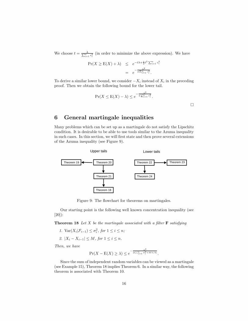
6 General martingale inequalities
Many problems which can be set up as a martingale do not satisfy the Lipschitzcondition. It is desirable to be able to use tools similar to the Azuma inequalityin such cases. In this section, we will first state and then prove several extensionsof the Azuma inequality (see Figure 9).
Theorem 20
Theorem 21
Theorem 18
Theorem 19 Theorem 22
Theorem 24
Theorem 23
Upper tails Lower tails
Figure 9: The flowchart for theorems on martingales.
Our starting point is the following well known concentration inequality (see[20]):
Theorem 18 Let X be the martingale associated with a filter F satisfying
1. Var(Xi|Fi−1) ≤ σ2i , for 1 ≤ i ≤ n;
2. |Xi − Xi−1| ≤ M , for 1 ≤ i ≤ n.
Then, we have
Pr(X − E(X) ≥ λ) ≤ e− λ2
2(Pn
i=1 σ2i+Mλ/3) .
Since the sum of independent random variables can be viewed as a martingale(see Example 15), Theorem 18 implies Theorem 6. In a similar way, the followingtheorem is associated with Theorem 10.
16
Theorem 19 Let X be the martingale associated with a filter F satisfying
1. Var(Xi|Fi−1) ≤ σ2i , for 1 ≤ i ≤ n;
2. Xi − Xi−1 ≤ Mi, for 1 ≤ i ≤ n.
Then, we have
Pr(X − E(X) ≥ λ) ≤ e− λ2
2Pn
i=1(σ2i+M2
i) .
The above theorem can be further generalized:
Theorem 20 Let X be the martingale associated with a filter F satisfying
1. Var(Xi|Fi−1) ≤ σ2i , for 1 ≤ i ≤ n;
2. Xi − Xi−1 ≤ ai + M , for 1 ≤ i ≤ n.
Then, we have
Pr(X − E(X) ≥ λ) ≤ e− λ2
2(Pn
i=1(σ2i+a2
i)+Mλ/3) .
Theorem 20 implies Theorem 18 by choosing a1 = a2 = · · · = an = 0.We also have the following theorem corresponding to Theorem 11.
Theorem 21 Let X be the martingale associated with a filter F satisfying
1. Var(Xi|Fi−1) ≤ σ2i , for 1 ≤ i ≤ n;
2. Xi − Xi−1 ≤ Mi, for 1 ≤ i ≤ n.
Then, for any M , we have
Pr(X − E(X) ≥ λ) ≤ e− λ2
2(Pn
i=1 σ2i+P
Mi>M (Mi−M)2+Mλ/3) .
Theorem 20 implies Theorem 21 by choosing
ai =
0 if Mi ≤ M,Mi − M if Mi ≥ M.
It suffices to prove Theorem 20 so that all the above stated theorems hold.Proof of Theorem 20:
Recall that g(y) = 2∑∞
k=2yk−2
k! satisfies the following properties:
• g(y) ≤ 1, for y < 0.
• limy→0 g(y) = 1.
• g(y) is monotone increasing, for y ≥ 0.
• When b < 3, we have g(b) ≤ 11−b/3 .
17
Since E(Xi|Fi−1) = Xi−1 and Xi − Xi−1 − ai ≤ M , we have
E(et(Xi−Xi−1−ai)|Fi−1) = E(∞∑
k=0
tk
k!(Xi − Xi−1 − ai)k|Fi−1)
= 1 − tai + E(∞∑
k=2
tk
k!(Xi − Xi−1 − ai)k|Fi−1)
≤ 1 − tai + E(t2
2(Xi − Xi−1 − ai)2g(tM)|Fi−1)
= 1 − tai +t2
2g(tM)E((Xi − Xi−1 − ai)2|Fi−1)
= 1 − tai +t2
2g(tM)(E((Xi − Xi−1)2|Fi−1) + a2
i )
≤ 1 − tai +t2
2g(tM)(σ2
i + a2i )
≤ e−tai+t22 g(tM)(σ2
i +a2i ).
Thus,
E(etXi |Fi−1) = E(et(Xi−Xi−1−ai)|Fi−1)etXi−1+tai
≤ e−tai+t22 g(tM)(σ2
i +a2i )etXi−1+tai
= et22 g(tM)(σ2
i +a2i )etXi−1 .
Inductively, we have
E(etX) = E(E(etXn |Fn−1))
≤ et22 g(tM)(σ2
n+a2n)E(etXn−1)
≤ · · ·
≤n∏
i=1
et22 g(tM)(σ2
i +a2i )E(etX0)
= e12 t2g(tM)
Pni=1(σ2
i +a2i )etE(X).
Then for t satisfying tM < 3, we have
Pr(X ≥ E(X) + λ) = Pr(etX ≥ etE(X)+tλ)≤ e−tE(X)−tλE(etX)
≤ e−tλe12 t2g(tM)
Pni=1(σ
2i +a2
i )
= e−tλ+ 12 t2g(tM)
Pni=1(σ
2i +a2
i )
≤ e−tλ+ 12
t21−tM/3
Pni=1(σ
2i +a2
i )
18
We choose t = λPni=1(σ2
i +a2i )+Mλ/3
. Clearly tM < 3 and
Pr(X ≥ E(X) + λ) ≤ e−tλ+ 12
t21−tM/3
Pni=1(σ
2i +a2
i )
= e− λ2
2(Pn
i=1(σ2i+a2
i)+Mλ/3) .
The proof of the theorem is complete. For completeness, we state the following theorems for the lower tails. The
proofs are almost identical and will be omitted.
Theorem 22 Let X be the martingale associated with a filter F satisfying
1. Var(Xi|Fi−1) ≤ σ2i , for 1 ≤ i ≤ n;
2. Xi−1 − Xi ≤ ai + M , for 1 ≤ i ≤ n.
Then, we have
Pr(X − E(X) ≤ −λ) ≤ e− λ2
2(Pn
i=1(σ2i+a2
i)+Mλ/3) .
Theorem 23 Let X be the martingale associated with a filter F satisfying
1. Var(Xi|Fi−1) ≤ σ2i , for 1 ≤ i ≤ n;
2. Xi−1 − Xi ≤ Mi, for 1 ≤ i ≤ n.
Then, we have
Pr(X − E(X) ≤ −λ) ≤ e− λ2
2Pn
i=1(σ2i+M2
i) .
Theorem 24 Let X be the martingale associated with a filter F satisfying
1. Var(Xi|Fi−1) ≤ σ2i , for 1 ≤ i ≤ n;
2. Xi−1 − Xi ≤ Mi, for 1 ≤ i ≤ n.
Then, for any M , we have
Pr(X − E(X) ≤ −λ) ≤ e− λ2
2(Pn
i=1 σ2i+P
Mi>M (Mi−M)2+Mλ/3) .
7 Supermartingales and Submartingales
In this section, we consider further strengthened versions of the martingaleinequalities that were mentioned so far. Instead of a fixed upper bound for thevariance, we will assume that the variance Var(Xi|Fi−1) is upper bounded by alinear function of Xi−1. Here we assume this linear function is non-negative forall values that Xi−1 takes. We first need some terminology.
For a filter F:∅, Ω = F0 ⊂ F1 ⊂ · · · ⊂ Fn = F ,
19
a sequence of random variables X0, X1, . . . , Xn is called a submartingale if Xi isFi-measurable (i.e., Xi(a) = Xi(b) if all elements of Fi containing a also containb and vice versa) then E(Xi | Fi−1) ≤ Xi−1, for 1 ≤ i ≤ n.
A sequence of random variables X0, X1, . . . , Xn is said to be a supermartin-gale if Xi is Fi-measurable and E(Xi | Fi−1) ≥ Xi−1, for 1 ≤ i ≤ n.
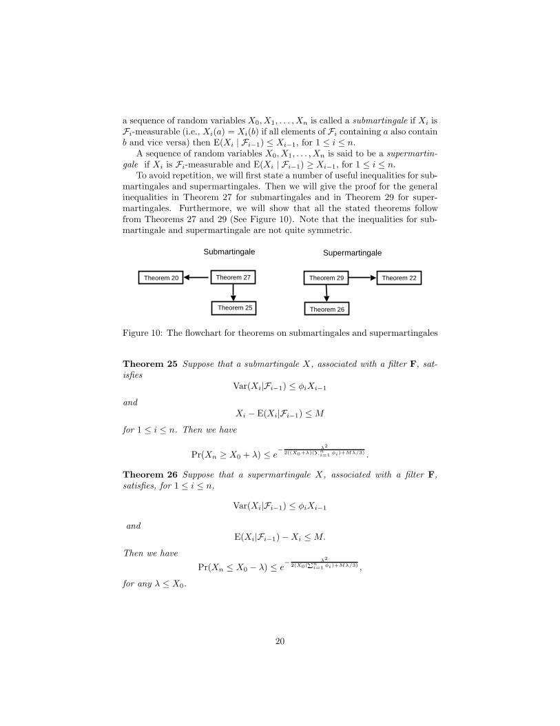
To avoid repetition, we will first state a number of useful inequalities for sub-martingales and supermartingales. Then we will give the proof for the generalinequalities in Theorem 27 for submartingales and in Theorem 29 for super-martingales. Furthermore, we will show that all the stated theorems followfrom Theorems 27 and 29 (See Figure 10). Note that the inequalities for sub-martingale and supermartingale are not quite symmetric.
Theorem 27
Theorem 25
Theorem 20 Theorem 29
Theorem 26
Theorem 22
Submartingale Supermartingale
Figure 10: The flowchart for theorems on submartingales and supermartingales
Theorem 25 Suppose that a submartingale X, associated with a filter F, sat-isfies
Var(Xi|Fi−1) ≤ φiXi−1
andXi − E(Xi|Fi−1) ≤ M
for 1 ≤ i ≤ n. Then we have
Pr(Xn ≥ X0 + λ) ≤ e− λ2
2((X0+λ)(Pn
i=1 φi)+Mλ/3) .
Theorem 26 Suppose that a supermartingale X, associated with a filter F,satisfies, for 1 ≤ i ≤ n,
Var(Xi|Fi−1) ≤ φiXi−1
andE(Xi|Fi−1) − Xi ≤ M.
Then we have
Pr(Xn ≤ X0 − λ) ≤ e− λ2
2(X0(Pn
i=1 φi)+Mλ/3) ,
for any λ ≤ X0.
20
Theorem 27 Suppose that a submartingale X, associated with a filter F, sat-isfies
Var(Xi|Fi−1) ≤ σ2i + φiXi−1
andXi − E(Xi|Fi−1) ≤ ai + M
for 1 ≤ i ≤ n. Here σi, ai, φi and M are non-negative constants. Then we have
Pr(Xn ≥ X0 + λ) ≤ e− λ2
2(Pn
i=1(σ2i+a2
i)+(X0+λ)(
Pni=1 φi)+Mλ/3) .
Remark 28 Theorem 27 implies Theorem 25 by setting all σi’s and ai’s tozero. Theorem 27 also implies Theorem 20 by choosing φ1 = · · · = φn = 0.
The theorem for a supermartingale is slightly different due to the asymmetryof the condition on the variance.
Theorem 29 Suppose a supermartingale X, associated with a filter F, satisfies,for 1 ≤ i ≤ n,
Var(Xi|Fi−1) ≤ σ2i + φiXi−1
andE(Xi|Fi−1) − Xi ≤ ai + M,
where M , ai’s, σi’s, and φi’s are non-negative constants. Then we have
Pr(Xn ≤ X0 − λ) ≤ e− λ2
2(Pn
i=1(σ2i+a2
i)+X0(
Pni=1 φi)+Mλ/3) ,
for any λ ≤ 2X0 +Pn
i=1(σ2i +a2
i )Pni=1 φi
.
Remark 30 Theorem 29 implies Theorem 26 by setting all σi’s and ai’s tozero. Theorem 29 also implies Theorem 22 by choosing φ1 = · · · = φn = 0.
Proof of Theorem 27:For a positive t (to be chosen later), we consider
E(etXi |Fi−1) = etE(Xi|Fi−1)+taiE(et(Xi−E(Xi|Fi−1)−ai)|Fi−1)
= etE(Xi|Fi−1)+tai
∞∑k=0
tk
k!E((Xi − E(Xi|Fi−1) − ai)k|Fi−1)
≤ etE(Xi|Fi−1)+P∞
k=2tk
k! E((Xi−E(Xi|Fi−1)−ai)k|Fi−1)
Recall that g(y) = 2∑∞
k=2yk−2
k! satisfies
g(y) ≤ g(b) <1
1 − b/3
for all y ≤ b and 0 ≤ b ≤ 3.
21
Since Xi − E(Xi|Fi−1) − ai ≤ M , we have
∞∑k=2
tk
k!E((Xi − E(Xi|Fi−1) − ai)k|Fi−1) ≤ g(tM)
2t2E((Xi − E(Xi|Fi−1) − ai)2|Fi−1)
=g(tM)
2t2(Var(Xi|Fi−1) + a2
i )
≤ g(tM)2
t2(σ2i + φiXi−1 + a2
i ).
Since E(Xi|Fi−1) ≤ Xi−1, we have
E(etXi |Fi−1) ≤ etE(Xi|Fi−1)+P∞
k=2tk
k! E((Xi−E(Xi|Fi−1−)−ai)k|Fi−1)
≤ etXi−1+g(tM)
2 t2(σ2i +φiXi−1+a2
i )
= e(t+ g(tM)2 φit
2)Xi−1et22 g(tM)(σ2
i +a2i ).
We define ti ≥ 0 for 0 < i ≤ n, satisfying
ti−1 = ti +g(t0M)
2φit
2i ,
while t0 will be chosen later. Then
tn ≤ tn−1 ≤ · · · ≤ t0,
and
E(etiXi |Fi−1) ≤ e(ti+g(tiM)
2 φit2i )Xi−1e
t2i2 g(tiM)(σ2
i +a2i )
≤ e(ti+g(t0M)
2 t2i φi)Xi−1et2i2 g(tiM)(σ2
i +a2i )
= eti−1Xi−1et2i2 g(tiM)(σ2
i +a2i )
since g(y) is increasing for y > 0.By Markov’s inequality, we have
Pr(Xn ≥ X0 + λ) ≤ e−tn(X0+λ)E(etnXn)= e−tn(X0+λ)E(E(etnXn |Fn−1))
≤ e−tn(X0+λ)E(etn−1Xn−1)et2i2 g(tiM)(σ2
i +a2i )
≤ · · ·≤ e−tn(X0+λ)E(et0X0)e
Pni=1
t2i2 g(tiM)(σ2
i +a2i )
≤ e−tn(X0+λ)+t0X0+t202 g(t0M)
Pni=1(σ
2i +a2
i ).
22
Note that
tn = t0 −n∑
i=1
(ti−1 − ti)
= t0 −n∑
i=1
g(t0M)2
φit2i
≥ t0 − g(t0M)2
t20
n∑i=1
φi.
Hence
Pr(Xn ≥ X0 + λ) ≤ e−tn(X0+λ)+t0X0+t202 g(t0M)
Pni=1(σ2
i +a2i )
≤ e−(t0− g(t0M)2 t20
Pni=1 φi)(X0+λ)+t0X0+
t202 g(t0M)
Pni=1(σ2
i +a2i )
= e−t0λ+g(t0M)
2 t20(Pn
i=1(σ2i +a2
i )+(X0+λ)Pn
i=1 φi)
Now we choose t0 = λPni=1(σ
2i +a2
i )+(X0+λ)(Pn
i=1 φi)+Mλ/3. Using the fact that
t0M < 3, we have
Pr(Xn ≥ X0 + λ) ≤ e−t0λ+t20(
Pni=1(σ2
i +a2i )+(X0+λ)
Pni=1 φi)
12(1−t0M/3)
= e− λ2
2(Pn
i=1(σ2i+a2
i)+(X0+λ)(
Pni=1 φi)+Mλ/3) .
The proof of the theorem is complete. Proof of Theorem 29:
The proof is quite similar to that of Theorem 27. The following inequalitystill holds.
E(e−tXi |Fi−1) = e−tE(Xi|Fi−1)+taiE(e−t(Xi−E(Xi|Fi−1)+ai)|Fi−1)
= e−tE(Xi|Fi−1)+tai
∞∑k=0
tk
k!E((E(Xi|Fi−1) − Xi − ai)k|Fi−1)
≤ e−tE(Xi|Fi−1)+P∞
k=2tk
k! E((E(Xi|Fi−1)−Xi−ai)k|Fi−1)
≤ e−tE(Xi|Fi−1)+g(tM)
2 t2E((Xi−E(Xi|Fi−1)−ai)2)
≤ e−tE(Xi|Fi−1)+g(tM)
2 t2(Var(Xi|Fi−1)+a2i )
≤ e−(t− g(tM)2 t2φi)Xi−1e
g(tM)2 t2(σ2
i +a2i ).
We now define ti ≥ 0, for 0 ≤ i < n satisfying
ti−1 = ti − g(tnM)2
φit2i .
tn will be defined later. Then we have
t0 ≤ t1 ≤ · · · ≤ tn,
23
and
E(e−tiXi |Fi−1) ≤ e−(ti− g(tiM)2 t2i φi)Xi−1e
g(tiM)2 t2i (σ2
i +a2i )
≤ e−(ti− g(tnM)2 t2i φi)Xi−1e
g(tnM)2 t2i (σ2
i +a2i )
= e−ti−1Xi−1eg(tnM)
2 t2i (σ2i +a2
i ).
By Markov’s inequality, we have
Pr(Xn ≤ X0 − λ) = Pr(−tnXn ≥ −tn(X0 − λ))≤ etn(X0−λ)E(e−tnXn)= etn(X0−λ)E(E(e−tnXn |Fn−1))
≤ etn(X0−λ)E(e−tn−1Xn−1)eg(tnM)
2 t2n(σ2n+a2
n)
≤ · · ·≤ etn(X0−λ)E(e−t0X0)e
Pni=1
g(tnM)2 t2i (σ2
i +a2i )
≤ etn(X0−λ)−t0X0+t2n2 g(tnM)
Pni=1(σ2
i +a2i ).
We note
t0 = tn +n∑
i=1
(ti−1 − ti)
= tn −n∑
i=1
g(tnM)2
φit2i
≥ tn − g(tnM)2
t2n
n∑i=1
φi.
Thus, we have
Pr(Xn ≤ X0 − λ) ≤ etn(X0−λ)−t0X0+t2n2 g(tnM)
Pni=1(σ
2i +a2
i )
≤ etn(X0−λ)−(tn− g(tnM)2 t2n)X0+
t2n2 g(tnM)
Pni=1(σ2
i +a2i )
= e−tnλ+ g(tnM)2 t2n(
Pni=1(σ
2i +a2
i )+(Pn
i=1 φi)X0)
We choose tn = λPni=1(σ
2i +a2
i )+(P
ni=1 φi)X0+Mλ/3
. We have tnM < 3 and
Pr(Xn ≤ X0 − λ) ≤ e−tnλ+t2n(Pn
i=1(σ2i +a2
i )+(Pn
i=1 φi)X0) 12(1−tnM/3)
≤ e− λ2
2(Pn
i=1(σ2i+a2
i)+X0(
Pni=1 φi)+Mλ/3) .
24
It remains to verify that all ti’s are non-negative. Indeed,
ti ≥ t0
≥ tn − g(tnM)2
t2n
n∑i=1
φi
≥ tn(1 − 12(1 − tnM/3)
tn
n∑i=1
φi)
= tn(1 − λ
2X0 +P
ni=1(σ
2i +a2
i )Pn
i=1 φi
)
≥ 0.
The proof of the theorem is complete.
8 The decision tree and relaxed concentrationinequalities
In this section, we will extend and generalize previous theorems to a martingalewhich is not strictly Lipschitz but is nearly Lipschitz. Namely, the (Lipschitz-like) assumptions are allowed to fail for relatively small subsets of the probabilityspace and we can still have similar but weaker concentration inequalities. Similartechniques have been introduced by Kim and Vu [19] in their important workon deriving concentration inequalities for multivariate polynomials. The basicsetup for decision trees can be found in [5] and has been used in the work ofAlon, Kim and Spencer [7]. Wormald [22] considers martingales with a ‘stoppingtime’ that has a similar flavor. Here we use a rather general setting and we shallgive a complete proof here.
We are only interested in finite probability spaces and we use the followingcomputational model. The random variable X can be evaluated by a sequenceof decisions Y1, Y2, . . . , Yn. Each decision has finitely many outputs. The proba-bility that an output is chosen depends on the previous history. We can describethe process by a decision tree T , a complete rooted tree with depth n. Eachedge uv of T is associated with a probability puv depending on the decisionmade from u to v. Note that for any node u, we have
∑v
pu,v = 1.
We allow puv to be zero and thus include the case of having fewer than r outputs,for some fixed r. Let Ωi denote the probability space obtained after the first idecisions. Suppose Ω = Ωn and X is the random variable on Ω. Let πi : Ω → Ωi
be the projection mapping each point to the subset of points with the samefirst i decisions. Let Fi be the σ-field generated by Y1, Y2, . . . , Yi. (In fact,Fi = π−1
i (2Ωi) is the full σ-field via the projection πi.) The Fi form a natural
25
filter:∅, Ω = F0 ⊂ F1 ⊂ · · · ⊂ Fn = F .
The leaves of the decision tree are exactly the elements of Ω. Let X0, X1, . . . , Xn =X denote the sequence of decisions to evaluate X . Note that Xi is Fi-measurable,and can be interpreted as a labeling on nodes at depth i.
There is one-to-one correspondence between the following:
• A sequence of random variables X0, X1, . . . , Xn satisfying Xi is Fi-measurable,for i = 0, 1, . . . , n.
• A vertex labeling of the decision tree T , f : V (T ) → R.
In order to simplify and unify the proofs for various general types of mar-tingales, here we introduce a definition for a function f : V (T ) → R. We say fsatisfies an admissible condition P if P = Pv holds for every vertex v.Examples of admissible conditions:
1. Supermartingale: For 1 ≤ i ≤ n, we have
E(Xi|Fi−1) ≥ Xi−1.
Thus the admissible condition Pu holds if
f(u) ≤∑
v∈C(u)
puvf(v)
where Cu is the set of all children nodes of u and puv is the transitionprobability at the edge uv.
2. Submartingale: For 1 ≤ i ≤ n, we have
E(Xi|Fi−1) ≤ Xi−1.
In this case, the admissible condition of the submartingale is
f(u) ≥∑
v∈C(u)
puvf(v).
3. Martingale: For 1 ≤ i ≤ n, we have
E(Xi|Fi−1) = Xi−1.
The admissible condition of the martingale is then:
f(u) =∑
v∈C(u)
puvf(v).
26
4. c-Lipschitz: For 1 ≤ i ≤ n, we have
|Xi − Xi−1| ≤ ci.
The admissible condition of the c-Lipschitz property can be described asfollows:
|f(u) − f(v)| ≤ ci, for any child v ∈ C(u)
where the node u is at level i of the decision tree.
5. Bounded Variance: For 1 ≤ i ≤ n, we have
Var(Xi|Fi−1) ≤ σ2i
for some constants σi.The admissible condition of the bounded variance property can be de-scribed as: ∑
v∈C(u)
puvf2(v) − (
∑v∈C(u)
puvf(v))2 ≤ σ2i .
6. General Bounded Variance: For 1 ≤ i ≤ n, we have
Var(Xi|Fi−1) ≤ σ2i + φiXi−1
where σi, φi are non-negative constants, and Xi ≥ 0. The admissiblecondition of the general bounded variance property can be described asfollows:∑
v∈C(u)
puvf2(v) − (
∑v∈C(u)
puvf(v))2 ≤ σ2i + φif(u), and f(u) ≥ 0
where i is the depth of the node u.
7. Upper-bound: For 1 ≤ i ≤ n, we have
Xi − E(Xi|Fi−1) ≤ ai + M
where ai’s, and M are non-negative constants. The admissible conditionof the upper bounded property can be described as follows:
f(v) −∑
v∈C(u)
puvf(v) ≤ ai + M, for any child v ∈ C(u)
where i is the depth of the node u.
8. Lower-bound: For 1 ≤ i ≤ n, we have
E(Xi|Fi−1) − Xi ≤ ai + M
where ai’s, and M are non-negative constants. The admissible conditionof the lower bounded property can be described as follows:
(∑
v∈C(u)
puvf(v)) − f(v) ≤ ai + M, for any child v ∈ C(u)
where i is the depth of the node u.
27
For any labeling f on T and fixed vertex r, we can define a new labeling fr
as follows:
fr(u) =
f(r) if u is a descedant of r.f(u) otherwise.
A property P is said to be invariant under subtree-unification if for any treelabeling f satisfying P , and a vertex r, fr satisfies P .
We have the following theorem.
Theorem 31 The eight properties as stated in the preceding examples — super-martingale, submartingale, martingale, c-Lipschitz, bounded variance, generalbounded variance, upper-bounded, and lower-bounded properties are all invari-ant under subtree-unification.
Proof: We note that these properties are all admissible conditions. Let Pdenote any one of these. For any node u, if u is not a descendant of r, then fr
and f have the same value on v and its children nodes. Hence, Pu holds for fr
since Pu does for f .If u is a descendant of r, then fr(u) takes the same value as f(r) as well as
its children nodes. We verify Pu in each case. Assume that u is at level i of thedecision tree T .
1. For supermartingale, submartingale, and martingale properties, we have∑
v∈C(u)
puvfr(v) =∑
v∈C(u)
puvf(r)
= f(r)∑
v∈C(u)
puv
= f(r)= fr(u).
Hence, Pu holds for fr.
2. For c-Lipschitz property, we have
|fr(u) − fr(v)| = 0 ≤ ci, for any child v ∈ C(u).
Again, Pu holds for fr.
3. For the bounded variance property, we have∑
v∈C(u)
puvf2r (v) − (
∑v∈C(u)
puvfr(v))2 =∑
v∈C(u)
puvf2(r) − (∑
v∈C(u)
puvf(r))2
= f2(r) − f2(r)= 0≤ σ2
i .
28

4. For the second bounded variance property, we have
fr(u) = f(r) ≥ 0.
∑v∈C(u)
puvf2r (v) − (
∑v∈C(u)
puvfr(v))2 =∑
v∈C(u)
puvf2(r) − (∑
v∈C(u)
puvf(r))2
= f2(r) − f2(r)= 0≤ σ2
i + φifr(u).
5. For upper-bounded property, we have
fr(v) −∑
v∈C(u)
puvfr(v) = f(r) −∑
v∈C(u)
puvf(r)
= f(r) − f(r)= 0≤ ai + M.
for any child v of u.
6. For the lower-bounded property, we have∑v∈C(u)
puvfr(v) − fr(v) =∑
v∈C(u)
puvf(r) − f(r)
= f(r) − f(r)= 0≤ ai + M,
for any child v of u.
Therefore, Pv holds for fr and any vertex v. .For two admissible conditions P and Q, we define PQ to be the property,
which is only true when both P and Q are true. If both admissible conditions Pand Q are invariant under subtree-unification, then PQ is also invariant undersubtree-unification.
For any vertex u of the tree T , an ancestor of u is a vertex lying on theunique path from the root to u. For an admissible condition P , the associatedbad set Bi over Xi’s is defined to be
Bi = v| the depth of v is i, and Pu does not hold for some ancestor u of v.Lemma 1 For a filter F
∅, Ω = F0 ⊂ F1 ⊂ · · · ⊂ Fn = F ,
suppose each random variable Xi is Fi-measurable, for 0 ≤ i ≤ n. For anyadmissible condition P , let Bi be the associated bad set of P over Xi. There arerandom variables Y0, . . . , Yn satisfying:
29
1. Yi is Fi-measurable.
2. Y0, . . . , Yn satisfy condition P .
3. x : Yi(x) 6= Xi(x) ⊂ Bi, for 0 ≤ i ≤ n.
Proof: We modify f and define f ′ on T as follows. For any vertex u,
f ′(u) =
f(u) if f satisfies Pv for every ancestor v of u including u itself,f(v) v is the ancestor with smallest depth so that f fails Pv.
Let S be the set of vertices u satisfying
• f fails Pu,
• f satisfies Pv for every ancestor v of u.
It is clear that f ′ can be obtained from f by a sequence of subtree-unifications,where S is the set of the roots of subtrees. Furthermore, the order of subtree-unifications does not matter. Since P is invariant under subtree-unifications,the number of vertices that P fails decreases. Now we will show f ′ satisfies P .
Suppose to the contrary that f ′ fails Pu for some vertex u. Since P isinvariant under subtree-unifications, f also fails Pu. By the definition, there isan ancestor v (of u) in S. After the subtree-unification on subtree rooted at v,Pu is satisfied. This is a contradiction.
Let Y0, Y1, . . . , Yn be the random variables corresponding to the labeling f ′.Yi’s satisfy the desired properties in (1)-(3).
The following theorem generalizes Azuma’s inequality. A similar but morerestricted version can be found in [19].
Theorem 32 For a filter F
∅, Ω = F0 ⊂ F1 ⊂ · · · ⊂ Fn = F ,
suppose the random variable Xi is Fi-measurable, for 0 ≤ i ≤ n. Let B = Bn
denote the bad set associated with the following admissible condition:
E(Xi|Fi−1) = Xi−1
|Xi − Xi−1| ≤ ci
for 1 ≤ i ≤ n where c1, c2, . . . , cn are non-negative numbers. Then we have
Pr(|Xn − X0| ≥ λ) ≤ 2e− λ2
2Pn
i=1 c2i + Pr(B),
Proof: We use Lemma 1 which gives random variables Y0, Y1, . . . , Yn satisfyingproperties (1)-(3) in the statement of Lemma 1. Then it satisfies
E(Yi|Fi−1) = Yi−1
|Yi − Yi−1| ≤ ci.
30
In other words, Y0, . . . , Yn form a martingale which is (c1, . . . , cn)-Lipschitz. ByAzuma’s inequality, we have
Pr(|Yn − Y0| ≥ λ) ≤ 2e− λ2
2Pn
i=1 c2i .
Since Y0 = X0 and x : Yn(x) 6= Xn(x) ⊂ Bn = B, we have
Pr(|Xn − X0| ≥ λ) ≤ Pr(|Yn − Y0| ≥ λ) + Pr(Xn 6= Yn)
≤ 2e− λ2
2Pn
i=1 c2i + Pr(B).
For c = (c1, c2, . . . , cn) a vector with positive entries, a martingale is said to
be near-c-Lipschitz with an exceptional probability η if∑
i
Pr(|Xi − Xi−1| ≥ ci) ≤ η. (6)
Theorem 32 can be restated as follows:
Theorem 33 For non-negative values, c1, c2, . . . , cn, suppose a martingale Xis near-c-Lipschitz with an exceptional probability η. Then X satisfies
Pr(|X − E(X)| < a) ≤ 2e− a2
2Pn
i=1 c2i + η.
Now, we can apply the same technique to relax all the theorems in theprevious sections.
Here are the relaxed versions of Theorems 20, 25, and 27.
Theorem 34 For a filter F
∅, Ω = F0 ⊂ F1 ⊂ · · · ⊂ Fn = F ,
suppose a random variable Xi is Fi-measurable, for 0 ≤ i ≤ n. Let B be thebad set associated with the following admissible conditions:
E(Xi | Fi−1) ≤ Xi−1
Var(Xi|Fi−1) ≤ σ2i
Xi − E(Xi|Fi−1) ≤ ai + M
for some non-negative constants σi and ai. Then we have
Pr(Xn ≥ X0 + λ) ≤ e− λ2
2(Pn
i=1(σ2i+a2
i)+Mλ/3) + Pr(B).
Theorem 35 For a filter F
∅, Ω = F0 ⊂ F1 ⊂ · · · ⊂ Fn = F ,
31
suppose a non-negative random variable Xi is Fi-measurable, for 0 ≤ i ≤ n.Let B be the bad set associated with the following admissible conditions:
E(Xi | Fi−1) ≤ Xi−1
Var(Xi|Fi−1) ≤ φiXi−1
Xi − E(Xi|Fi−1) ≤ M
for some non-negative constants φi and M . Then we have
Pr(Xn ≥ X0 + λ) ≤ e− λ2
2((X0+λ)(Pn
i=1 φi)+Mλ/3) + Pr(B).
Theorem 36 For a filter F
∅, Ω = F0 ⊂ F1 ⊂ · · · ⊂ Fn = F ,
suppose a non-negative random variable Xi is Fi-measurable, for 0 ≤ i ≤ n.Let B be the bad set associated with the following admissible conditions:
E(Xi | Fi−1) ≤ Xi−1
Var(Xi|Fi−1) ≤ σ2i + φiXi−1
Xi − E(Xi|Fi−1) ≤ ai + M
for some non-negative constants σi, φi, ai and M . Then we have
Pr(Xn ≥ X0 + λ) ≤ e− λ2
2(Pn
i=1(σ2i+a2
i)+(X0+λ)(
Pni=1 φi)+Mλ/3) + Pr(B).
For supermartingales, we have the following relaxed versions of Theorem 22,26, and 29.
Theorem 37 For a filter F
∅, Ω = F0 ⊂ F1 ⊂ · · · ⊂ Fn = F ,
suppose a random variable Xi is Fi-measurable, for 0 ≤ i ≤ n. Let B be thebad set associated with the following admissible conditions:
E(Xi | Fi−1) ≥ Xi−1
Var(Xi|Fi−1) ≤ σ2i
E(Xi|Fi−1) − Xi ≤ ai + M
for some non-negative constants σi, ai and M . Then we have
Pr(Xn ≤ X0 − λ) ≤ e− λ2
2(Pn
i=1(σ2i+a2
i)+Mλ/3) + Pr(B).
Theorem 38 For a filter F
∅, Ω = F0 ⊂ F1 ⊂ · · · ⊂ Fn = F ,
32

suppose a random variable Xi is Fi-measurable, for 0 ≤ i ≤ n. Let B be thebad set associated with the following admissible conditions:
E(Xi | Fi−1) ≥ Xi−1
Var(Xi|Fi−1) ≤ φiXi−1
E(Xi|Fi−1) − Xi ≤ M
for some non-negative constants φi and M . Then we have
Pr(Xn ≤ X0 − λ) ≤ e− λ2
2(X0(Pn
i=1 φi)+Mλ/3) + Pr(B).
for all λ ≤ X0.
Theorem 39 For a filter F
∅, Ω = F0 ⊂ F1 ⊂ · · · ⊂ Fn = F ,
suppose a non-negative random variable Xi is Fi-measurable, for 0 ≤ i ≤ n.Let B be the bad set associated with the following admissible conditions:
E(Xi | Fi−1) ≥ Xi−1
Var(Xi|Fi−1) ≤ σ2i + φiXi−1
E(Xi|Fi−1) − Xi ≤ ai + M
for some non-negative constants σi,φi, ai and M . Then we have
Pr(Xn ≤ X0 − λ) ≤ e− λ2
2(Pn
i=1(σ2i+a2
i)+X0(
Pni=1 φi)+Mλ/3) + Pr(B),
for λ < X0.
9 A generalized Polya’s urn problem
To see the powerful effect of the concentration and martingale inequalities inthe previous sections, the best way is to check out some interesting applications.In the this section we give the probabilistic analysis of the following processinvolving balls and bins:
For a fixed 0 ≤ p < 1 and a positive integer κ > 1, begin with κ bins,each containing one ball and then introduce balls one at a time. Foreach new ball, with probability p, create a new bin and place theball in that bin; otherwise, place the ball in an existing bin, suchthat the probability the ball is placed in a bin is proportional to thenumber of balls in that bin.
Polya’s urn problem (see [18]) is a special case of the above process withp = 0 so new bins are never created. For the case of p > 0, this infinite Polya
33
process has a similar flavor as the preferential attachment scheme, one of themain models for generating the webgraph among other information networks(see Barabasi et al [4, 6]).
In Subsection 9.1, we will show that the infinite Polya process generatesa power law distribution so that the expected fraction of bins having k ballsis asymptotic to ck−β , where β = 1 + 1/(1 − p) and c is a constant. Thenthe concentration result on the probabilistic error estimates for the power lawdistribution will be given in Subsection 9.2.
9.1 The expected number of bins with k balls
To analyze the infinite Polya process, we let nt denote the number of bins attime t and let et denote the number of balls at time t. We have
et = t + κ.
The number of bins nt, however, is a sum of t random indicator variables,
nt = κ +t∑
i=1
st
where
Pr(sj = 1) = p,
Pr(sj = 0) = 1 − p.
It follows thatE(nt) = κ + pt.
To get a handle on the actual value of nt, we use the binomial concentrationinequality as described in Theorem 4. Namely,
Pr(|nt − E(nt)| > a) ≤ e−a2/(2pt+2a/3).
Thus, nt is exponentially concentrated around E(nt).The problem of interest is the distribution of sizes of bins in the infinite
Polya process.Let mk,t denote the number of bins with k balls at time t. First we note
thatm1,0 = κ, and m0,k = 0.
We wish to derive the recurrence for the expected value E(mk,t). Note thata bin with k balls at time t could have come from two cases, either it was a binwith k balls at time t− 1 and no ball was added to it, or it was a bin with k− 1balls at time t−1 and a new ball was put in. Let Ft be the σ-algebra generatedby all the possible outcomes at time t.
E(mk,t|Ft−1) = mk,t−1(1 − (1 − p)kt + κ
) + mk−1,t−1((1 − p)(k − 1)
t + κ − 1)
E(mk,t) = E(mk,t−1)(1 − (1 − p)kt + κ − 1
) + E(mk−1,t−1)((1 − p)(k − 1)
t + κ − 1).(7)
34
For t > 0 and k = 1, we have
E(m1,t|Ft−1) = m1,t−1(1 − (1 − p)t + κ − 1
) + p.
E(m1,t) = E(m1,t−1)(1 − (1 − p)t + κ − 1
) + p. (8)
To solve this recurrence, we use the following fact (see [12]):For a sequence at satisfying the recursive relation at+1 = (1 − bt
t )at + ct,limt→∞ at
t exists and
limt→∞
at
t=
c
1 + b
provided that limt→∞ bt = b > 0 and limt→∞ ct = c.We proceed by induction on k to show that limt→∞ E(mk,t)/t has a limit
Mk for each k.The first case is k = 1. In this case, we apply the above fact with bt = b =
1 − p and ct = c = p to deduce that limt→∞ E(m1,t)/t exists and
M1 = limt→∞
E(m1,t)t
=p
2 − p.
Now we assume that limt→∞ E(mk−1,t)/t exists and we apply the fact againwith bt = b = k(1 − p) and ct = E(mk−1,t−1)(1 − p)(k − 1)/(t + κ − 1), soc = Mk−1(1− p)(k− 1). Thus the limit limt→∞ E(mk,t)/t exists and is equal to
Mk = Mk−1(1 − p)(k − 1)1 + k(1 − p)
= Mk−1k − 1
k + 11−p
. (9)
Thus we can write
Mk =p
2 − p
k∏j=2
j − 1j + 1
1−p
=p
2 − p
Γ(k)Γ(2 + 11−p )
Γ(k + 1 + 11−p )
where Γ(k) is the Gamma function.We wish to show that the distribution of the bin sizes follows a power law
with Mk ∝ k−β (where ∝ means “is proportional to”) for large k. If Mk ∝ k−β ,then
Mk
Mk−1=
k−β
(k − 1)−β= (1 − 1
k)β = 1 − β
k+ O(
1k2
).
From (9) we have
Mk
Mk−1=
k − 1k + 1
1−p
= 1 − 1 + 11−p
k + 11−p
= 1 − 1 + 11−p
k+ O(
1k2
).
Thus we have an approximate power-law with
β = 1 +1
1 − p= 2 +
p
1 − p.
35
9.2 Concentration on the number of bins with k balls
Since the expected value can be quite different from the actual number of binswith k balls at time t, we give a (probabilistic) estimate of the difference.
We will prove the following theorem.
Theorem 40 For the infinite Polya process, asymptotically almost surely thenumber of bins with k balls at time t is
Mk(t + κ) + O(2√
k3(t + κ) ln(t + κ)).
Recall M1 = p2−p and Mk = p
2−p
Γ(k)Γ(2+ 11−p )
Γ(k+1+ 11−p )
= O(k−(2+ p1−p )), for k ≥ 2. In
other words, almost surely the distribution of the bin sizes for the infinite Polyaprocess follows a power law with the exponent β = 1 + 1
1−p .
Proof: We have shown that
limt→∞
E(mk,t)t
= Mk,
where Mk is defined recursively in (9). It is sufficient to show mk,t concentrateson the expected value.
We shall prove the following claim.
Claim: For any fixed k ≥ 1, for any c > 0, with probability at least 1 − 2(t +κ + 1)k−1e−c2
, we have
|mk,t − Mk(t + κ)| ≤ 2kc√
t + κ.
To see that the claim implies Theorem 40, we choose c =√
k ln(t + κ). Notethat
2(t + κ)k−1e−c2= 2(t + κ + 1)k−1(t + κ)−k = o(1).
From the claim, with probability 1 − o(1), we have
|mk,t − Mk(t + κ)| ≤ 2√
k3(t + κ) ln(t + κ),
as desired.It remains to prove the claim.
Proof of the Claim: We shall prove it by induction on k.
The base case of k = 1:For k = 1, from equation (8), we have
E(m1,t − M1(t + κ)|Ft−1)= E(m1,t|Ft−1) − M1(t + κ)
= m1,t−1(1 − 1 − p
t + κ − 1) + p − M1(t + κ − 1) − M1
= (m1,t−1 − M1(t + κ − 1))(1 − 1 − p
t + κ − 1) + p − M1(1 − p) − M1
= (m1,t−1 − M1(t + κ − 1))(1 − 1 − p
t + κ − 1)
36
since p − M1(1 − p) − M1 = 0.Let X1,t = m1,t−M1(t+κ)
Qtj=1(1− 1−p
j+κ−1 ). We consider the martingale formed by 1 =
X1,0, X1,1, . . . , X1,t. We have
X1,t − X1,t−1
=m1,t − M1(t + κ)∏t
j=1(1 − 1−pj+κ−1 )
− m1,t−1 − M1(t + κ − 1)∏t−1j=1(1 − 1−p
j+κ−1 )
=1∏t
j=1(1 − 1−pj+κ−1 )
[(m1,t − M1(t + κ)) − (m1,t−1 − M1(t + κ − 1))(1 − 1 − p
t + κ − 1)]
=1∏t
j=1(1 − 1−pj+κ−1 )
[(m1,t − m1,t−1) +1 − p
t + κ − 1(m1,t−1 − M1(t + κ − 1)) − M1].
We note that |m1,t − m1,t−1| ≤ 1, m1,t−1 ≤ t, and M1 = p2−p < 1. We have
|X1,t − X1,t−1| ≤ 1∏tj=1(1 − 1−p
j+κ−1 ). (10)
Since |m1,t − m1,t−1| ≤ 1, we have
Var(m1,t|Ft−1) ≤ E((m1,t − m1,t−1)2|Ft−1)≤ 1.
Therefore, we have the following upper bound for Var(X1,t|Ft−1).
Var(X1,t|Ft−1) = Var((m1,t − M1(t + κ))
1∏tj=1(1 − 1−p
j+κ−1 )
∣∣Ft−1
)
=1∏t
j=1(1 − 1−pj+κ−1 )2
Var(m1,t − M1(t + κ)|Ft−1)
=1∏t
j=1(1 − 1−pj+κ−1 )2
Var(m1,t|Ft−1)
≤ 1∏tj=1(1 − 1−p
j+κ−1 )2. (11)
We apply Theorem 19 on the martingale X1,t with σ2i = 4Q
ij=1(1− 1−p
j+κ−1 )2,
M = 4Qtj=1(1− 1−p
j+κ−1 )and ai = 0. We have
Pr(X1,t ≥ E(X1,t) + λ) ≤ e− λ2
2(Pt
i=1 σ2i+Mλ/3) .
37
Here E(X1,t) = X1,0 = 1. We will use the following approximation.
i∏j=1
(1 − 1 − p
j + κ − 1) =
i∏j=1
j + κ − 2 + p
j + κ − 1
=Γ(κ)Γ(i + κ − 1 + p)Γ(κ − 1 + p)Γ(i + κ)
≈ C(i + κ)−1+p
where C = Γ(κ)Γ(κ−1+p) is a constant depending only on p and κ.
For any c > 0, we choose λ = 4c√
t+κQ
tj=1(1− 1−p
j )≈ 4C−1ct3/2−p. We have
t∑i=1
σ2i =
t∑i=1
4∏ij=1(1 − 1−p
j )2
≈t∑
i=1
4C−2(i + κ)2−2p
≈ 4C−2
3 − 2p(t + κ)3−2p
< 4C−2(t + κ)3−2p.
We note thatMλ/3 ≈ 8
3C−2ct5/2−2p < 2C−2t3−2p
provided 4c/3 <√
t + κ. We have
Pr(X1,t ≥ 1 + λ) ≤ e− λ2
2(Pt
i=1 σ2i+Mλ/3)
< e− 16C−2c2t3−2p
8C−2t3−2p+2C−2(t+κ)3−2p
< e−c2.
Since 1 is much smaller than λ, we can replace 1 + λ by 1 without loss ofgenerality. Thus, with probability at least 1 − e−c2
, we have
X1,t ≤ λ.
Similarly, with probability at least 1 − e−c2, we have
m1,t − M1(t + κ) ≤ 2c√
t + κ. (12)
We remark that inequality (12) holds for any c > 0. In fact, it is trivial when4c/3 >
√t + κ since |m1,t − M1(t + κ)| ≤ 2t always holds.
Similarly, by applying Theorem 23 on the martingale, the following lowerbound
m1,t − M1(t + κ) ≥ −2c√
t + κ (13)
38
holds with probability at least 1 − e−c2.
We have proved the claim for k = 1.The inductive step:
Suppose the claim holds for k − 1. For k, we define
Xk,t =mk,t − Mk(t + κ) − 2(k − 1)c
√t + κ∏t
j=1(1 − (1−p)kj+κ−1 )
.
We have
E(mk,t − Mk(t + κ) − 2(k − 1)c√
t + κ|Ft−1)= E(mk,t|Ft−1) − Mk(t + κ) − 2(k − 1)c
√t + κ
= mk,t−1(1 − (1 − p)kt + κ − 1
) + mk−1,t−1((1 − p)(k − 1)
t + κ − 1)
−Mk(t + κ) − 2(k − 1)c√
t + κ.
By the induction hypothesis, with probability at least 1− 2tk−2e−c2, we have
|mk−1,t−1 − Mk−1(t + κ)| ≤ 2(k − 1)c√
t + κ.
By using this estimate, with probability at least 1 − 2tk−2e−c2, we have
E(mk,t − Mk(t + κ) − 2(k − 1)c√
t + κ|Ft−1)
≤ (1 − (1 − p)kt
)(mk,t−1 − Mk(t + κ − 1) − 2(k − 1)c√
t + κ − 1)
from the fact that Mk ≤ Mk−1 as seen in (9).Therefore, 0 = Xk,0, Xk,1, · · · , Xk,t forms a submartingale with failure prob-
ability at most 2tk−2e−c2.
Similar to inequalities (10) and (11), it can be easily shown that
|Xk,t − Xk,t−1| ≤ 4∏tj=1(1 − (1−p)k
j+κ−1 )(14)
and
Var(Xk,t|Ft−1) ≤ 4∏tj=1(1 − (1−p)k
j+κ−1 )2.
We apply Theorem 35 on the submartingale with σ2i = 4
Qij=1(1− (1−p)k
j+κ−1 )2,
M = 4Qt
j=1(1− (1−p)κj+κ−1 )
and ai = 0. We have
Pr(Xk,t ≥ E(Xk,t) + λ) ≤ e− λ2
2(Pt
i=1 σ2i+Mλ/3) + Pr(B),
where Pr(B) ≤ tk−1e−c2by induction hypothesis.
39
Here E(Xk,t) = Xk,0 = 0. We will use the following approximation.
i∏j=1
(1 − (1 − p)kj + κ − 1
) =i∏
j=1
j − (1 − p)kj + κ − 1
=Γ(κ)
Γ(1 − (1 − p)k)Γ(i + 1 − (1 − p)k)
Γ(i + κ)
≈ Ck(i + κ)−(1−p)k
where Ck = Γ(κ)Γ(1−(1−p)k) is a constant depending only on k, p and κ.
For any c > 0, we choose λ = 4c√
t+κQt
j=1(1− (1−p)kj )
≈ 4C−1k ct3/2−p. We have
t∑i=1
σ2i =
t∑i=1
4∏ij=1(1 − (1−p)k
j )2
≈t∑
i=1
4C−2k (i + κ)2k(1−p)
≈ 4C−2k
1 + 2k(1 − p)(t + κ)1+2k(1−p)
< 4C−2k (t + κ)1+2k(1−p).
We note that
Mλ/3 ≈ 83C−2
k c(t + κ)1/2+2(1−p) < 2C−2k (t + κ)1+2(1−p)
provided 4c/3 <√
t + κ. We have
Pr(Xk,t ≥ λ) ≤ e− λ2
2(Pt
i=1 σ2i+Mλ/3) + Pr(B)
< e− 16C
−2k
c2(t+κ)1+2k(1−p)
8C−2k
(t+κ)1+2(1−p)+2C−2k
(t+κ)1+2(1−p) + Pr(B)
< e−c2+ (t + κ)k−1e−c2
≤ (t + κ + 1)k−1e−c2.
With probability at least 1 − (t + κ + 1)k−1e−c2, we have
Xk,t ≤ λ.
Equivalently, with probability at least 1 − (t + κ + 1)k−1e−c2, we have
mk,t − Mk(t + κ) ≤ 2ck√
t + κ. (15)
We remark that inequality (15) holds for any c > 0. In fact, it is trivial when4c/3 >
√t + κ since |mk,t − Mk(t + κ)| ≤ 2(t + κ) always holds.
40
To obtain the lower bound, we consider
X ′k,t =
mk,t − Mk(t + κ) + 2(k − 1)c√
t + κ∏tj=1(1 − (1−p)k
j+κ−1 ).
It can be easily shown that X ′k,t is nearly a supermartingale. Similarly, if ap-
plying Theorem 38 to X ′k,t, the following lower bound
mk,t − Mk(t + κ) ≥ −2kc√
t + κ (16)
holds with probability at least 1 − (t + κ + 1)k−1e−c2.
Together these prove the statement for k. The proof of Theorem 40 iscomplete.
The above methods for proving concentration of the power law distributionfor the infinite Polya process can be easily carried out for many other problems.One of the most popular models for generating random graphs (which simu-late webgraphs and various information networks) is the so-called preferentialattachment scheme. The problem on the degree distribution of the preferentialattachment scheme can be viewed as a variation of the Polya process as we willsee. Before we proceed, we first give a short description for the preferentialattachment scheme [3, 21]:
• With probability p, for some fixed p, add a new vertex v, and add an edgeu, v from v by randomly and independently choosing u in proportion tothe degree of u in the current graph. The initial graph, say, is one singlevertex with a loop.
• Otherwise, add a new edge r, s by independently choosing vertices r ands with probability proportional to their degrees. Here r and s could bethe same vertex.
The above preferential attachment scheme can be rewritten as the followingvariation of the Polya process:
• Start with one bin containing one ball.
• At each step, with probability p, add two balls, one to a new bin andone to an existing bin with probability proportional to the bin size. withprobability 1 − p, add two balls, each of which is independently placed toan existing bin with probability proportional to the bin size.
As we can see, the bins are the vertices; at each time step the bins thatthe two balls are placed are associated with an edge; the bin size is exactly thedegree of the vertex.
It is not difficult to show the expected degrees of the preferential attachmentmodel satisfy a power law distribution with exponent 1 + 2/(2 − p) (see [3,21]). The concentration results for the power law degree distribution of thepreferential attachment scheme can be proved in a very similar way as what wehave done in this section for the Polya process. The details of the proof can befound in a forthcoming book [13].
41
References
[1] J. Abello, A. Buchsbaum, and J. Westbrook, A functional approach toexternal graph algorithms, Proc. 6th European Symposium on Algorithms,pp. 332–343, 1998.
[2] W. Aiello, F. Chung and L. Lu, A random graph model for massive graphs,Proceedings of the Thirty-Second Annual ACM Symposium on Theory ofComputing, (2000) 171-180.
[3] W. Aiello, F. Chung and L. Lu, Random evolution in massive graphs,Extended abstract appeared in The 42th Annual Symposium on Foundationof Computer Sciences, October, 2001. Paper version appeared in Handbookof Massive Data Sets, (Eds. J. Abello, et. al.), Kluwer Academic Publishers(2002), 97-122.
[4] R. Albert and A.-L. Barabasi, Statistical mechanics of complex networks,Review of Modern Physics 74 (2002), 47-97.
[5] N. Alon and J. H. Spencer, The Probabilistic Method, Wiley and Sons, NewYork, 1992.
[6] A.-L. Barabasi and R. Albert, Emergence of scaling in random networks,Science 286 (1999) 509-512.
[7] N. Alon, J.-H. Kim and J. H. Spencer, Nearly perfect matchings in regularsimple hypergraphs, Israel J. Math. 100 (1997), 171-187.
[8] H. Chernoff, A note on an inequality involving the normal distribution,Ann. Probab., 9, (1981), 533-535.
[9] F. Chung and L. Lu, Connected components in random graphs with givenexpected degree sequences, Annals of Combinatorics 6, (2002), 125–145.
[10] F. Chung and L. Lu, The average distances in random graphs with givenexpected degrees, Proceeding of National Academy of Science 99, (2002),15879–15882.
[11] F. Chung, L. Lu and V. Vu, The spectra of random graphs with givenexpected degrees, Proceedings of National Academy of Sciences, 100, no.11, (2003), 6313-6318.
[12] F. Chung and L. Lu, Coupling online and offline analyses for random powerlaw graphs, Internet Mathematics, 1 (2004), 409-461.
[13] F. Chung and L. Lu, Complex Graphs and Networks, CBMS Lecture Notes,in preparation.
[14] F. Chung, S. Handjani and D. Jungreis, Generalizations of Polya’s urnproblem, Annals of Combinatorics, 7, (2003), 141-153.
42
[15] W. Feller, Martingales, An Introduction to Probability Theory and its Ap-plications, Vol. 2, New York, Wiley, 1971.
[16] R. L. Graham, D. E. Knuth and O. Patashnik, Concrete Mathematics,Second edition, Addison-Wesley Publishing Company, Reading, MA, 1994.
[17] S. Janson, T. Luczak, and A. Rucınski, Random Graphs, Wiley-Interscience, New York, 2000.
[18] N. Johnson and S. Kotz, Urn Models and their Applications: An approachto Modern Discrete Probability Theory, Wiley, New York, 1977.
[19] J. H. Kim and V. Vu, Concentration of multivariate polynomials and itsapplications, Combinatorica, 20 (3) (2000), 417-434.
[20] C. McDiarmid, Concentration, Probabilistic methods for algorithmic dis-crete mathematics, 195–248, Algorithms Combin., 16, Springer, Berlin,1998.
[21] M. Mitzenmacher, A brief history of generative models for power law andlognormal distribution, Internet Mathematics, 1, (2004), 226-251.
[22] N. C. Wormald, The differential equation method for random processesand greedy algorithms, in Lectures on Approximation and Randomized Al-gorithms, (M. Karonski and H. J. Proemel, eds), pp. 73-155, PWN, Warsaw,1999.
43


![Martingale techniques · 2014-10-28 · 3.1.3 Martingales 3.1.4 . Percolation on trees: critical regime To be written. See [Per09, Sections 2 and 3]. 3.2 Concentration for martingales](https://img.pdfslide.us/doc/110x75/5f519c630eb6cb08b030e5ce/martingale-techniques-2014-10-28-313-martingales-314-percolation-on-trees.jpg)