Embed Size (px)
Citation preview

6. Martingales
• For casino gamblers, a martingale is a betting
strategy where (at even odds) the stake doubled
each time the player loses. Players follow this
strategy because, since they will eventually win,
they argue they are guaranteed to make money!
• A stochastic process {Zn, n ≥ 1} is a
martingale if E[
|Zn|]
< ∞ and
E[
Zn+1 |Z1, . . . , Zn
]
= Zn.
• Think of Zn+1 as being a gambler’s earnings
after n+ 1 games. If the game if fair, then
E[
Zn+1 |Zn
]
= Zn. This is true whatever stake
the gambler places-the stake at game n+ 1 can
depend on Z1, . . . , Zn.
• We will show that no strategy can guarantee
success at a fair game. This is a generalization of
Wald’s equation.
1

• Since martingales can have rather general
dependence (the only constraint is an conditional
expectations), they are a powerful tool for
dependent stochastic processes.
• Identifying an embedded martingale can lead to
elegant solutions.
Examples
(i) Suppose X1, X2, . . . are iid, mean µ. Then
Zn =∑n
i=1(Xi − µ) is a Martingale. Why?
(ii) Product martingale. If X1, X2, . . . are iid
with mean 1, then Zn =∏n
i=1 Xi is a martingale.
Why?
2

(iii) Martingale differences. Let X1, X2, . . . be
arbitrary dependent random variables with
E[
|Xi|]
< ∞ and E[
Xk |X1, . . . , Xk−1
]
= 0.
Then Zn =∑n
i=1 Xi is a martingale. Why?
• Correspondingly, for any martingale {Zn} we
can construct martingale differences
Xk = Zk − Zk−1
• In particular, for any sequence X1, X2, . . .,
Zn =∑n
i=1
{
Xi − E[
Xi |X1, . . . Xi−1
]}
is a
martingale. Why?
3

(iv) Let E[
|X|]
< ∞ and take Y1, Y2, . . . to be
arbitrary random variables. Set
Zn = E[
X |Y1, . . . , Yn
]
. Then Zn is a Martingale.
Why?
(v) Continuous-time martingales. Z(t) is a
martingale in continuous time if E[
|Z(t)|]
< ∞
and E[
Z(t) |Z(u), 0 ≤ u ≤ s]
= Z(s) for s < t.
We will not study the continuous time case
thoroughly, but similar results apply.
• If N(t) is a rate λ Poisson counting process,
Z(t) = N(t)− λt is a martingale.
4

• If N(t) is a general renewal process, then
N(t)−m(t) is not a Martingale. Why? Find a
related process which is a Martingale.
• Identify a Martingale corresponding to a
continuous time birth-death process, X(t), with
rates λn and µn.
5
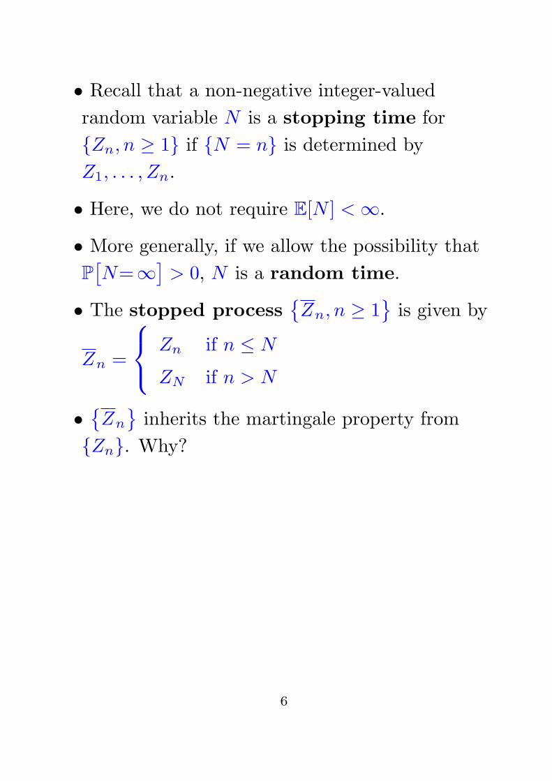
• Recall that a non-negative integer-valued
random variable N is a stopping time for
{Zn, n ≥ 1} if {N = n} is determined by
Z1, . . . , Zn.
• Here, we do not require E[N ] < ∞.
• More generally, if we allow the possibility that
P[
N=∞]
> 0, N is a random time.
• The stopped process{
Zn, n ≥ 1}
is given by
Zn =
Zn if n ≤ N
ZN if n > N
•{
Zn
}
inherits the martingale property from
{Zn}. Why?
6

Solution continued
7

Theorem (Martingale Stopping Theorem)
If N is a stopping time for a martingale {Zn}
then E[
ZN
]
= E[
Z1
]
, provided one of the
following conditions is satisfied:
(i) Zn is uniformly bounded (i.e., there exist a
and b with a< Zn<b whenever n ≤ N).
(ii) N is bounded.
(iii) E[N ] < ∞ and, for some M < ∞,
E[
|Zn+1 − Zn|∣
∣Z1, . . . , Zn
]
< M .
Proof
8

Example: What does the stopping theorem
imply about the “martingale” betting strategy
(keep doubling the stakes until you win, then
eventually you are guaranteed to make a profit).
Example: A gambler plays a fair game at even
odds, each play results in winning/losing $1 with
probability 1/2. The gambler starts with $ a and
stops when he goes broke or reaches $ b. Find the
chance of reaching $ b.
9

Example: Expected time to see a given pattern.
A monkey hits random letters on a keyboard.
What is the expected number of hits until typing
ABRACADABRA.
Solution
10

Convergence of Martingales
• A useful property of martingales is that, if their
expected absolute value is uniformly bounded,
they converge with probability 1.
• To develop these ideas, we first study some
inequalities.
Definition If {Zn, n ≥ 1} is a stochastic process
with E[
|Zn|]
< ∞ then it is a
submartingale if E[
Zn+1 |Z1, . . . , Zn
]
≥ Zn
supermartingale if E[
Zn+1 |Z1, . . . , Zn
]
≤ Zn
• Most casino games are super martingales, as far
as the player is concerned, i.e., subfair. Allegedly,
there are systems to make the player’s winnings
at blackjack a submartingale, i.e., superfair.
• Note that the definition implies
E[
Zn+1
]
≥ E[
Zn
]
for a submartingale.
E[
Zn+1
]
≤ E[
Zn
]
for a supermartingale.
11

Example: If f is a convex function and {Zn} is
a martingale, then {f(Zn)} is a submartingale.
Proof. We need to use Jensen’s inequality: If
f is a convex function, then E[f(X)] ≥ f(E[X]).
12

Stopping for Sub(Super) Martingales
If N is a stopping time for {Zn} satisfying any of
the conditions for the martingale stopping
theorem,
E[
ZN
]
≥ E[
Z1
]
for a submartingale
E[
ZN
]
≤ E[
Z1
]
for a supermartingale
(1)
If furthermore, N is bounded, say N ≤ n, then
E[
Zn
]
≥ E[
ZN
]
≥ E[
Z1
]
submartingale
E[
Zn
]
≤ E[
ZN
]
≤ E[
Z1
]
supermartingale
(2)
Proof. For the submartingale case, how does (1)
follow from the martingale stopping theorem?
How does (2) follow from (1)?
13

Proof continued
14

Kolmogorov’s submartingale inequality
If {Zn} is a non-negative submartingale, then
P[
max(Z1, . . . , Zn) ≥ a]
≤ E[Zn]a
for a > 0.
• Note that Jensen’s inequality then gives, for any
martingale {Zn},
P[
max( |Z1| , . . . , |Zn| ) ≥ a]
≤ E[
|Zn|]/
a
and
P[
max( |Z1| , . . . , |Zn| ) ≥ a]
≤ E[
Z2n
]/
a2.
Proof of the submartingale inequality
15

Example: An urn initially contains one white
and one black ball. At each stage a ball is drawn,
and is then replaced in the urn along with another
ball of the same color. Let Zn be the fraction of
white balls in the urn after the nth iteration.
(a) Show that {Zn} is a martingale.
(b) Show that the probability that the fraction of
white balls is ever as large as 3/4 is at most 2/3.
16

Martingale Convergence Theorem
If {Zn, n ≥ 1} is a martingale and E[
|Zn|]
≤ M
then, with probability 1, limn→∞ Zn exists and is
finite.
• Note: write Z∞ = limn→∞ Zn. This limit is
generally random, but Z∞ may sometimes be a
constant. This theorem asserts that for (almost)
every outcome s in the sample space S,
limn→∞ Zn(s) = Z∞(s).
• Note that the theorem applies to any
non-negative martingale, since then
E[
|Zn|]
= E[Zn] = E[Z1].
Proof
17

Proof continued
18

Example: Let {Zn, n ≥ 1} be a sequence of
random variables such that Z1 = 1 and, given
Z1, . . . , Zn−1, the distribution of Zn is
conditionally Poisson with mean Zn−1 for n > 1.
What happens to Zn as n gets large?
19

Example: Let Xn be the population size of the
nth generation of a branching process, with each
individual having, on average, m offspring.
Describe the behavior of Xn for large n.
20
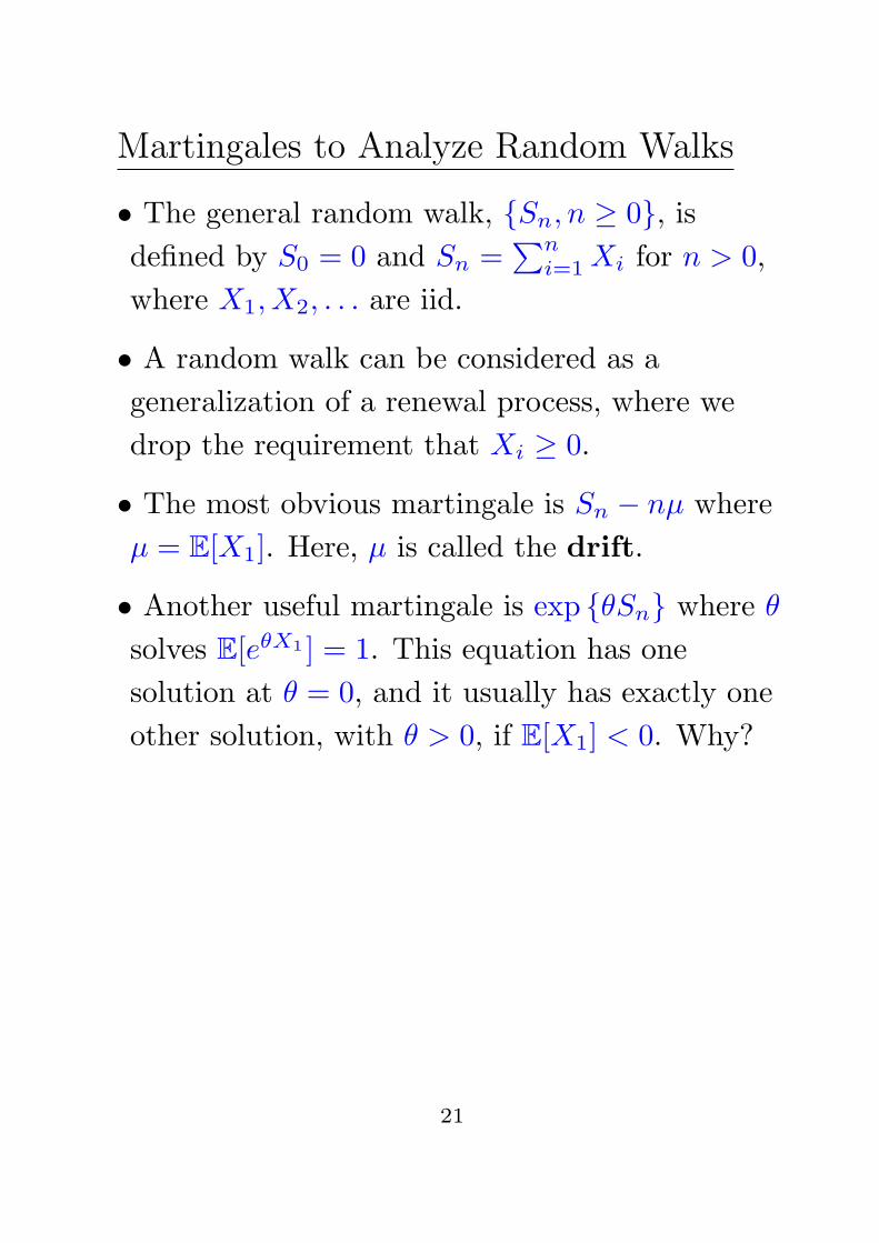
Martingales to Analyze Random Walks
• The general random walk, {Sn, n ≥ 0}, is
defined by S0 = 0 and Sn =∑n
i=1 Xi for n > 0,
where X1, X2, . . . are iid.
• A random walk can be considered as a
generalization of a renewal process, where we
drop the requirement that Xi ≥ 0.
• The most obvious martingale is Sn − nµ where
µ = E[X1]. Here, µ is called the drift.
• Another useful martingale is exp {θSn} where θ
solves E[eθX1 ] = 1. This equation has one
solution at θ = 0, and it usually has exactly one
other solution, with θ > 0, if E[X1] < 0. Why?
21
Example: Let N= min {n : Sn≥A or Sn≤−B}.
Use martingale arguments to find (approximately)
P[SN ≥ A] and E[N ].
• Note: this models a general situation where we
accumulate rewards, and at some point we quit
and declare failure (if SN ≤ −B), or quit having
achieved our goal (if SN ≥ A). An example is
sequential analysis of clinical trails.
Solution
22

Solution continued
23