Embed Size (px)
Citation preview

Lecture Notes — Probability Theory
Manuel Cabral Morais
Department of Mathematics
Instituto Superior Tecnico
Lisbon, Sep. 2009/10 — Jan. 2010/11 (Revised in Jul./Dec. 2014)
Contents
0. Warm up 1
0.1 Historical note . . . . . . . . . . . . . . . . . . . . . . . . . . . . . . . . . . 1
0.2 (Symmetric) random walk . . . . . . . . . . . . . . . . . . . . . . . . . . . 2
1 Probability spaces 12
1.1 Random experiments . . . . . . . . . . . . . . . . . . . . . . . . . . . . . . 16
1.2 Events and classes of sets . . . . . . . . . . . . . . . . . . . . . . . . . . . . 19
1.3 Probabilities and probability functions . . . . . . . . . . . . . . . . . . . . 31
1.4 Distribution functions; discrete, absolutely continuous and mixed
probabilities . . . . . . . . . . . . . . . . . . . . . . . . . . . . . . . . . . . 39
1.5 Conditional probability . . . . . . . . . . . . . . . . . . . . . . . . . . . . . 50
2 Random variables 56
2.1 Fundamentals . . . . . . . . . . . . . . . . . . . . . . . . . . . . . . . . . . 56
2.2 Combining random variables . . . . . . . . . . . . . . . . . . . . . . . . . . 63
2.3 Distributions and distribution functions . . . . . . . . . . . . . . . . . . . . 66
2.4 Key r.v. and random vectors and distributions . . . . . . . . . . . . . . . . 70
2.4.1 Discrete r.v. and random vectors . . . . . . . . . . . . . . . . . . . 70
2.4.2 Absolutely continuous r.v. and random vectors . . . . . . . . . . . . 75
2.5 Transformation theory . . . . . . . . . . . . . . . . . . . . . . . . . . . . . 82
2.5.1 Transformations of r.v., general case . . . . . . . . . . . . . . . . . 82
2.5.2 Transformations of discrete r.v. . . . . . . . . . . . . . . . . . . . . 84
2.5.3 Transformations of absolutely continuous r.v. . . . . . . . . . . . . 86
2.5.4 Transformations of random vectors, general case . . . . . . . . . . . 92
2.5.5 Transformations of discrete random vectors . . . . . . . . . . . . . . 92
2.5.6 Transformations of absolutely continuous random vectors . . . . . . 98
2.5.7 Random variables with prescribed distributions . . . . . . . . . . . 105
ii
3 Independence 111
3.1 Fundamentals . . . . . . . . . . . . . . . . . . . . . . . . . . . . . . . . . . 111
3.2 Independent r.v. . . . . . . . . . . . . . . . . . . . . . . . . . . . . . . . . . 116
3.3 Functions of independent r.v. . . . . . . . . . . . . . . . . . . . . . . . . . 121
3.4 Order statistics . . . . . . . . . . . . . . . . . . . . . . . . . . . . . . . . . 126
3.5 Constructing independent r.v. . . . . . . . . . . . . . . . . . . . . . . . . . 130
3.6 Bernoulli process . . . . . . . . . . . . . . . . . . . . . . . . . . . . . . . . 131
3.7 Poisson process . . . . . . . . . . . . . . . . . . . . . . . . . . . . . . . . . 136
3.8 Generalizations of the Poisson process . . . . . . . . . . . . . . . . . . . . . 143
4 Expectation 147
4.1 Definition and fundamental properties . . . . . . . . . . . . . . . . . . . . 148
4.1.1 Simple r.v. . . . . . . . . . . . . . . . . . . . . . . . . . . . . . . . . 148
4.1.2 Non negative r.v. . . . . . . . . . . . . . . . . . . . . . . . . . . . . 152
4.1.3 Integrable r.v. . . . . . . . . . . . . . . . . . . . . . . . . . . . . . . 157
4.1.4 Complex r.v. . . . . . . . . . . . . . . . . . . . . . . . . . . . . . . 159
4.2 Integrals with respect to distribution functions . . . . . . . . . . . . . . . . 160
4.2.1 On integration . . . . . . . . . . . . . . . . . . . . . . . . . . . . . 160
4.2.2 Generalities . . . . . . . . . . . . . . . . . . . . . . . . . . . . . . . 163
4.2.3 Discrete distribution functions . . . . . . . . . . . . . . . . . . . . . 165
4.2.4 Absolutely continuous distribution functions . . . . . . . . . . . . . 165
4.2.5 Mixed distribution functions . . . . . . . . . . . . . . . . . . . . . . 166
4.3 Computation of expectations . . . . . . . . . . . . . . . . . . . . . . . . . . 167
4.3.1 Non negative r.v. . . . . . . . . . . . . . . . . . . . . . . . . . . . . 167
4.3.2 Integrable r.v. . . . . . . . . . . . . . . . . . . . . . . . . . . . . . . 168
4.3.3 Mixed r.v. . . . . . . . . . . . . . . . . . . . . . . . . . . . . . . . . 169
4.3.4 Functions of r.v. . . . . . . . . . . . . . . . . . . . . . . . . . . . . . 171
4.3.5 Functions of random vectors . . . . . . . . . . . . . . . . . . . . . . 172
4.3.6 Functions of independent r.v. . . . . . . . . . . . . . . . . . . . . . 173
4.3.7 Sum of independent r.v. . . . . . . . . . . . . . . . . . . . . . . . . 174
4.4 Lp spaces . . . . . . . . . . . . . . . . . . . . . . . . . . . . . . . . . . . . 176
4.5 Key inequalities . . . . . . . . . . . . . . . . . . . . . . . . . . . . . . . . . 177
4.5.1 Young’s inequality . . . . . . . . . . . . . . . . . . . . . . . . . . . 178
4.5.2 Holder’s moment inequality . . . . . . . . . . . . . . . . . . . . . . 179
4.5.3 Cauchy-Schwarz’s moment inequality . . . . . . . . . . . . . . . . . 181
4.5.4 Lyapunov’s moment inequality . . . . . . . . . . . . . . . . . . . . . 182
iii
4.5.5 Minkowski’s moment inequality . . . . . . . . . . . . . . . . . . . . 183
4.5.6 Jensen’s moment inequality . . . . . . . . . . . . . . . . . . . . . . 184
4.5.7 Chebyshev’s inequality . . . . . . . . . . . . . . . . . . . . . . . . . 186
4.6 Moments . . . . . . . . . . . . . . . . . . . . . . . . . . . . . . . . . . . . . 190
4.6.1 Moments of r.v. . . . . . . . . . . . . . . . . . . . . . . . . . . . . . 190
4.6.2 Variance and standard deviation . . . . . . . . . . . . . . . . . . . . 192
4.6.3 Skewness and kurtosis . . . . . . . . . . . . . . . . . . . . . . . . . 194
4.6.4 Covariance . . . . . . . . . . . . . . . . . . . . . . . . . . . . . . . . 196
4.6.5 Correlation . . . . . . . . . . . . . . . . . . . . . . . . . . . . . . . 198
4.6.6 Moments of random vectors . . . . . . . . . . . . . . . . . . . . . . 202
4.6.7 Multivariate normal distributions . . . . . . . . . . . . . . . . . . . 203
4.6.8 Multinomial distributions . . . . . . . . . . . . . . . . . . . . . . . 216
5 Convergence concepts and classical limit theorems 224
5.1 Modes of convergence . . . . . . . . . . . . . . . . . . . . . . . . . . . . . . 225
5.1.1 Convergence of r.v. as functions on ! . . . . . . . . . . . . . . . . . 225
5.1.2 Convergence in distribution . . . . . . . . . . . . . . . . . . . . . . 232
5.1.3 Alternative criteria . . . . . . . . . . . . . . . . . . . . . . . . . . . 238
5.2 Relationships among the modes of convergence . . . . . . . . . . . . . . . . 242
5.2.1 Implications always valid . . . . . . . . . . . . . . . . . . . . . . . . 242
5.2.2 Counterexamples . . . . . . . . . . . . . . . . . . . . . . . . . . . . 244
5.2.3 Implications of restricted validity . . . . . . . . . . . . . . . . . . . 247
5.3 Convergence under transformations . . . . . . . . . . . . . . . . . . . . . . 249
5.3.1 Continuous mappings . . . . . . . . . . . . . . . . . . . . . . . . . . 249
5.3.2 Algebraic operations . . . . . . . . . . . . . . . . . . . . . . . . . . 249
5.4 Convergence of random vectors . . . . . . . . . . . . . . . . . . . . . . . . 256
5.5 Limit theorems for Bernoulli summands . . . . . . . . . . . . . . . . . . . 259
5.5.1 Laws of large numbers for Bernoulli summands . . . . . . . . . . . 259
5.5.2 Central limit theorems for Bernoulli summands . . . . . . . . . . . 262
5.5.3 The Poisson limit theorem . . . . . . . . . . . . . . . . . . . . . . . 264
5.6 Weak law of large numbers . . . . . . . . . . . . . . . . . . . . . . . . . . . 267
5.7 Strong law of large numbers . . . . . . . . . . . . . . . . . . . . . . . . . . 273
5.8 Characteristic functions . . . . . . . . . . . . . . . . . . . . . . . . . . . . 275
5.9 The Central Limit Theorem . . . . . . . . . . . . . . . . . . . . . . . . . . 283
5.10 The law of the iterated logarithm . . . . . . . . . . . . . . . . . . . . . . . 287
5.11 Applications of the limit theorems . . . . . . . . . . . . . . . . . . . . . . . 289
iv

Warm up
0.1 Historical note
Mathematical probability has its origins in games of chance [...]. Early
calculations involving dice were included in a well-known and widely distributed
poem entitled De Vetula.1 Dice and cards continued as the main vessels of
gambling in the 15th. and 16th. centuries [...]. [...] (G. Cardano) went so far
as to write a book, On games of chance, sometime shortly after 1550. This was
not published however until 1663, by which time probability theory had already
had its o!cial inauguration elsewhere.
It was around 1654 that B. Pascal and P. de Fermat generated a celebrated
correspondence about their solutions of the problem of the points. These were
soon widely known, and C. Huygens developed these ideas in a book published
in 1657, in Latin. [...] the intuitive notions underlying this work were similar
to those commonly in force nowdays.
These first simple ideas were soon extended by Jacob Bernoulli in Ars
conjectandi (1713) and by A. de Moivre in Doctrine of chances (1718, 1738,
1756). [...]. Methods, results, and ideas were all greatly refined and generalized
by P. Laplace [...]. Many other eminent mathematicians of this period wrote
on probability: Euler, Gauss, Lagrange, Legendre, Poisson, and so on.
However, as ever harder problems were tackled by ever more powerful
mathematical techniques during the 19th. century, the lack of a well-defined
axiomatic structure was recognized as a serious handicap. [...] A. Kolmogorov
provided the axioms which today underpin most mathematical probability.
Grimmett and Stirzaker (2001, p. 571)
1De vetula (”The Old Woman”) is a long thirteenth-century poem written in Latin. (For more detailssee http://en.wikipedia.org/wiki/De vetula.)
1
For more extensive and exciting accounts on the history of Statistics and Probability,
we recommend:
• Hald, A. (1998). A History of Mathematical Statistics from 1750 to 1930. John
Wiley & Sons. (QA273-280/2.HAL.50129);
• Stigler, S.M. (1986). The History of Statistics: the Measurement of Uncertainty
Before 1900. Belknap Press of Harvard University Press. (QA273-280/2.STI.39095).
0.2 (Symmetric) random walk
This section is inspired by Karr (1993, pp. 1–14) and has
the sole purpose of:
• illustrating concepts such as probability, random
variables, independence, expectation and
convergence of random sequences, and recall
some limit theorems;
• drawing our attention to the fact that exploiting
the special structure of a random process can
provide answers for some of the questions raised.
It refers to the random walk, a mathematical
formalization of path that consist of a succession of
random steps (http://en.wikipedia.org/wiki/Random walk), such as the ones portrayed
above.
The term random walk was first introduced by Karl Pearson in 1905
(http://en.wikipedia.org/wiki/Random walk).
Informal definition 0.1 — Symmetric random walk
The symmetric random walk (SRW) is a random experiment which can result from the
observation of a particle moving randomly on Z = {. . . ,!1, 0, 1, . . .}. Moreover, the
particle starts at the origin at time 0, and then moves either one step up or one step down
with equal likelihood. •
2

Remark 0.2 — Applications of random walk
The path followed by atom in a gas moving under the influence of collisions with other
atoms can be described by a random walk (RW). Random walk has also been applied in
other areas such as:
• economics (RW used to model shares prices and other factors);
• population genetics (RW describes the statistical properties of genetic drift);2
• mathematical ecology (RW used to describe individual animal movements, to
empirically support processes of biodi"usion, and occasionally to model population
dynamics);
• computer science (RW used to estimate the size of the Web);
• visual arts, such as Antony Gormley’s Quantum Cloud sculpture in London which
was designed by a computer using a random walk algorithm.3
•
The next proposition provides answers to the following questions:
• How can we model and analize the symmetric random walk?
• What random variables can arise from this random experiment and how can we
describe them?
2Genetic drift is one of several evolutionary processes which lead to changes in allele frequencies overtime.
3For more applications check http://en.wikipedia.org/wiki/Random walk.
3
Proposition 0.3 — Symmetric random walk (Karr, 1993, pp. 1–4)
1. The model
Let:
• !n be the step at time n (!n = ±1);
• ! = (!1, !2, . . .) be a realization of the random walk;
• ! be the sample space of the random experiment, i.e. the set of all possible
realizations.
2. Random variables
Two random variables immediately arise:
• Yn defined as Yn(!) = !n, the size of the nth step;4
• Xn which represents the position at time n and is defined as
Xn(!) =!n
i=1 Yi(!).
A realization of {Yn, n " N} and the corresponding sample path of {Xn, n " N}are shown below for p = 1
2 .
1 2 3 4 5 6 7 8t
!1
1
1 2 3 4 5 6 7 8t
!4
!3
!2
!1
0
1
2
3
4
3. Probability and independence
The sets of outcomes of this random experiment are termed events. An event A # !
occurs with probability P (A).
Recall that a probability function is countable additive, i.e. for sequences of
(pairwise) disjoint events A1, A2, . . . (Ai $ Aj = %, i &= j) we have
P
"+!#
i=1
Ai
$=
+!%
i=1
P (Ai). (1)
4Steps are functions defined on the sample space. Thus, steps are random variables.
4
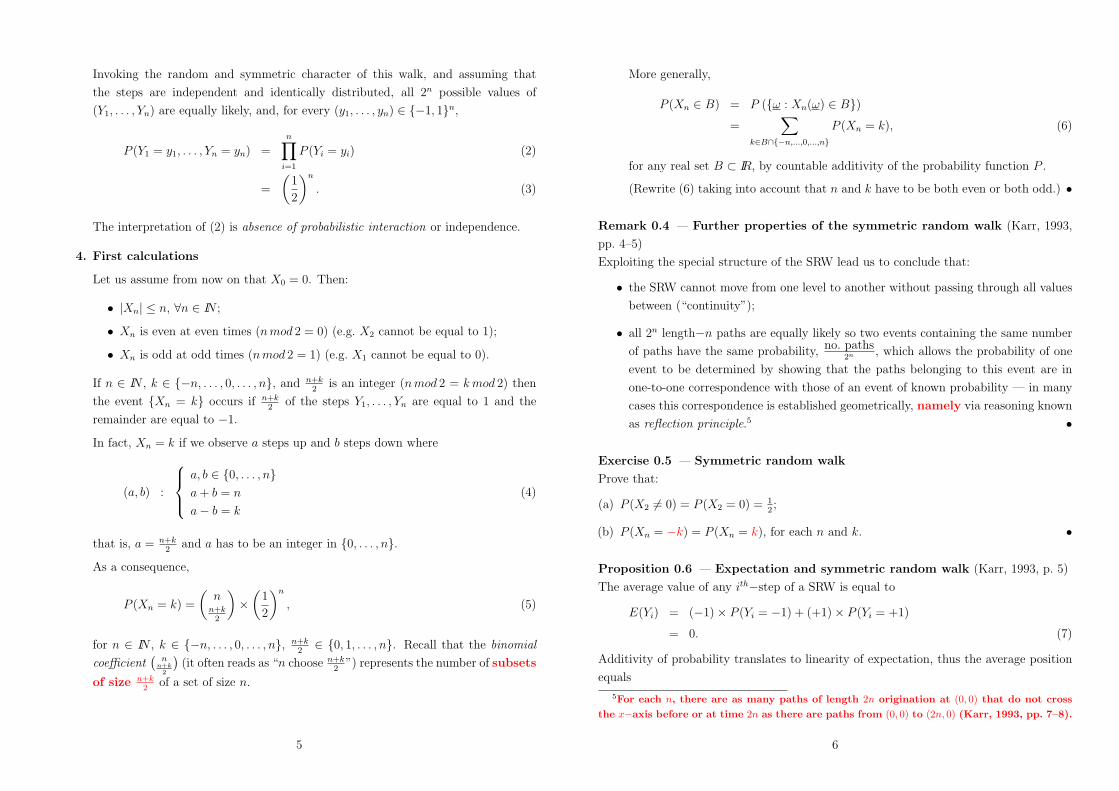
Invoking the random and symmetric character of this walk, and assuming that
the steps are independent and identically distributed, all 2n possible values of
(Y1, . . . , Yn) are equally likely, and, for every (y1, . . . , yn) " {!1, 1}n,
P (Y1 = y1, . . . , Yn = yn) =n&
i=1
P (Yi = yi) (2)
=
'1
2
(n
. (3)
The interpretation of (2) is absence of probabilistic interaction or independence.
4. First calculations
Let us assume from now on that X0 = 0. Then:
• |Xn| ' n, (n " IN ;
• Xn is even at even times (n mod 2 = 0) (e.g. X2 cannot be equal to 1);
• Xn is odd at odd times (n mod 2 = 1) (e.g. X1 cannot be equal to 0).
If n " IN , k " {!n, . . . , 0, . . . , n}, and n+k2 is an integer (n mod 2 = k mod 2) then
the event {Xn = k} occurs if n+k2 of the steps Y1, . . . , Yn are equal to 1 and the
remainder are equal to !1.
In fact, Xn = k if we observe a steps up and b steps down where
(a, b) :
)*+
*,
a, b " {0, . . . , n}a + b = n
a! b = k
(4)
that is, a = n+k2 and a has to be an integer in {0, . . . , n}.
As a consequence,
P (Xn = k) =
'n
n+k2
()
'1
2
(n
, (5)
for n " IN , k " {!n, . . . , 0, . . . , n}, n+k2 " {0, 1, . . . , n}. Recall that the binomial
coe!cient-
nn+k
2
.(it often reads as “n choose n+k
2 ”) represents the number of subsets
of size n+k2 of a set of size n.
5
More generally,
P (Xn " B) = P ({! : Xn(!) " B})=
%
k"B#{$n,...,0,...,n}
P (Xn = k), (6)
for any real set B # IR, by countable additivity of the probability function P .
(Rewrite (6) taking into account that n and k have to be both even or both odd.) •
Remark 0.4 — Further properties of the symmetric random walk (Karr, 1993,
pp. 4–5)
Exploiting the special structure of the SRW lead us to conclude that:
• the SRW cannot move from one level to another without passing through all values
between (“continuity”);
• all 2n length!n paths are equally likely so two events containing the same number
of paths have the same probability, no. paths2n , which allows the probability of one
event to be determined by showing that the paths belonging to this event are in
one-to-one correspondence with those of an event of known probability — in many
cases this correspondence is established geometrically, namely via reasoning known
as reflection principle.5 •
Exercise 0.5 — Symmetric random walk
Prove that:
(a) P (X2 &= 0) = P (X2 = 0) = 12 ;
(b) P (Xn = !k) = P (Xn = k), for each n and k. •
Proposition 0.6 — Expectation and symmetric random walk (Karr, 1993, p. 5)
The average value of any ith!step of a SRW is equal to
E(Yi) = (!1)) P (Yi = !1) + (+1)) P (Yi = +1)
= 0. (7)
Additivity of probability translates to linearity of expectation, thus the average position
equals
5For each n, there are as many paths of length 2n origination at (0, 0) that do not crossthe x!axis before or at time 2n as there are paths from (0, 0) to (2n, 0) (Karr, 1993, pp. 7–8).
6

E(Xn) = E
"n%
i=1
Yi
$
=n%
i=1
E(Yi)
= 0. (8)
•
Proposition 0.7 — Conditioning and symmetric random walk (Karr, 1993, p. 6)
We can revise probability in light of the knowledge that some event has occurred. For
example, we know that P (X2n = 0) =-2nn
.)
-12
.2n. However, if we knew that X2n$1 = 1
then the event {X2n = 0} occurs with probability 12 . In fact,
P (X2n = 0|X2n$1 = 1) =P (X2n$1 = 1, X2n = 0)
P (X2n$1 = 1)
=P (X2n$1 = 1, Y2n = !1)
P (X2n$1 = 1)
=P (X2n$1 = 1)) P (Y2n = !1)
P (X2n$1 = 1)
=1
2. (9)
Note that, since the steps Yi are independent random variables and X2n$1 =!2n$1
i=1 Yi,
we can state that Y2n is independent of X2n$1. •
Exercise 0.8 — Conditioning and asymmetric random walk6
Random walk models are often found in physics, from particle motion to a simple
description of a polymer.
A physicist assumes that the position of a particle at time n, Xn, is governed by
an asymmetric random walk — starting at 0 and with probability of an upward (resp.
downward) step equal to p (resp. 1! p), where p " (0, 1)\{12}.
Derive P (X2n = 0|X2n$2 = 0), for n = 2, 3, . . . •
Proposition 0.9 — Time of first return to the origin and symmetric random
walk (Karr, 1993, pp. 7-9)
The time at which the SRW first returns to the origin,
6Exam 2010/01/19.
7
T 0 = min{n " IN : Xn = 0}, (10)
is an important functional of the SRW (it maps the SRW into a scalar). It can represent
the time to ruin.
Interestingly enough, for n " IN , T 0 must be a positive and even r.v. (recall that
X0 = 0). And, for n " IN :
P (T 0 > 2n) = P (X1 &= 0, . . . , X2n &= 0) =
'2n
n
()
'1
2
(2n
; (11)
P (T 0 = 2n) =1
2n! 1
'2n
n
()
'1
2
(2n
. (12)
Moreover, using the Stirling’s approximation to n!, n! *+
2" nn+ 12 e$n, we get
P (T 0 < +,) = 1. (13)
If we note that P (T 0 > 2n) * 1%!n and recall that
!+!n=1
1ns only converges for s - 2,
we can conclude that T 0 assumes large values with probabilities large enough that
+!%
n=1
2n P (T 0 = 2n) = +,. E(T 0) = +,. (14)
•
Exercise 0.10 — Time of first return to the origin and symmetric random walk
(a) Prove result (12) using (11).
(b) Use the Stirling’s approximation to n!, n! *+
2" nn+ 12 e$n to prove that
limn&+!
P (T 0 > 2n) = limn&+!
1+"n
.
(c) Use the previous result and the fact that
P (T 0 < +,) = 1! limn&+!
P (T 0 > 2n)
to derive (13).
(d) Verify that!+!
n=1 2n P (T 0 = 2n) = 1 +!+!
n=1 P (T 0 > 2n), even though we have
E(Z) = 2 )/1 +
!+!n=1 P (Z > 2n)
0, for any positive and even random variable Z
with finite expected value E(Z) =!+!
n=1 2n) P (Z = 2n). •
8

Proposition 0.11 — First passage times and symmetric random walk (Karr,
1993, pp. 9–11)
Similarly, the first passage time
T k = min{n " IN : Xn = k}, (15)
has the following properties, for n " IN , k " {!n, . . . ,!1, 1, . . . , n} and n mod 2 =
k mod 2:
P (T k = n) =|k|n) P (Xn = k); (16)
P (T k < ,) = 1; (17)
E(T k) = +,. (18)
•
The following results pertain to the asymptotic behaviour of the position of a
symmetric random walk and to the fraction of time spent positive.
Proposition 0.12 — Law of large numbers (Karr, 1993, p. 12)
Let Yn and Xn =!n
i=1 Yi represent the size of the nth. step and the position at time n
of a random walk, respectively. Then
P
'lim
n&+!
Xn
n= 0
(= 1, (19)
that is, the “empirical averages”, Xnn = 1
n
!ni=1 Yi, converge to the “theoretical average”
E(Y1). •
Proposition 0.13 — Central limit theorem (Karr, 1993, pp. 12–13)
limn&+!
P
1
2Xnn ! E
-Xnn
.3
V-
Xnn
. ' x
4
5 = limn&+!
P
1
2Xnn ! E(Y1)3
V (Y1)n
' x
4
5
=
6 x
$!
1+2"
e$y2
2 dy
= #(x), x " IR. (20)
So, for large values of n, di$cult-to-compute probabilities can be approximated. For
instance, for a < b, we get:
9
P (a < Xn ' b) =%
a<k'b
P (Xn = k)
= P
1
2an ! 03
1n
<Xnn ! 03
1n
'bn ! 03
1n
4
5
* #(b/+
n)! #(a/+
n). (21)
•
Exercise 0.14 — Central limit theorem7
The words “symmetric random walk” refer to this situation.
The proverbial drunk (PD) is clinging to the lamppost. He decides to start
walking. The road runs east and west. In his inebriated state he is as likely
to take a step east (forward) as west (backward). In each new position he is
again as likely to go forward as backward. Each of his steps are of the same
length but of random direction — east or west.
http://www.physics.ucla.edu//chester/TECH/RandomWalk/3Pane.html
Admit that each step of PD has length equal to one meter and that he has already taken
exactly 100 (a hundred) steps.
Find an approximate value for the probability that PD is within a five meters
neighborhood of the lamppost. •
Proposition 0.15 — Arc sine law (Karr, 1993, pp. 13–14)
The fraction of time spent positive Wnn = 1
n
!ni=1 IIN(Xi +Xi$1) has the following limiting
law:8
limn&+!
P
'Wn
n' x
(=
2
"arcsin
+x. (22)
Moreover, the associated limiting density function, 1
!+
x(1$x), is a U!shaped density.
Thus, Wnn is more likely to be near 0 or 1 than near 1/2.
7Exam 2010/02/04.8According to Karr (1993, p. 12), being positive at time i requires that either Xi > 0 or Xi!1 > 0 (or
both).
10

Please note that we can get the limiting distribution function by using the Stirling’s
approximation and the following result:
P (W2n = 2k) =
'2k
k
()
'2n! 2k
n! k
()
'1
2
(2n
. (23)
•
Exercise 0.16 — Arc sine law
Prove result (22) (Karr, 1993, p. 13). •
Exercise 0.17 — Arc sine law9
The random walk hypothesis is due to French economist Louis Bachelier (1870–1946) and
asserts that the random nature of a commodity or stock prices cannot reveal trends and
therefore current prices are no guide to future prices. Surprisingly, an investor assumes
that his/her daily financial score is governed by a symmetric random walk starting at 0.
Obtain the corresponding approximate value for the probability that the fraction of
time the financial score is positive exceeds 50%. •
Exercise 0.18 — The cli!-hanger problem (Mosteller, 1965, pp. 51–54)
From where he stands (X0 = 1), one step toward the cli" would send the drunken man
over the edge. He takes random steps, either toward or away from the cli". At any step,
his probability of taking a step away is p and of a step toward the cli" 1! p.
What is his chance of not escaping the cli"? (Write the results in terms of p.) •
References
• Grimmett, G.R. and Stirzaker, D.R. (2001). Probability and Random Processes
(3rd. edition). Oxford. (QA274.12-.76.GRI.40695 refers to the library code of the
1st. and 2nd. editions from 1982 and 1992, respectively.)
• Karr, A.F. (1993). Probability. Springer-Verlag.
• Konstantopoulos, T. (2009). Introductory Lecture Notes on Markov Chains and
Random Walks. (www2.math.uu.se//takis/L/McRw/mcrw.pdf)
• Mosteller, F. (1965). Fifty Challenging Problems in Probability with Solutions.
Dover Publications.
9Test 2009/11/07.
11
Chapter 1
Probability spaces
[...] have been taught that the universe evolves according to deterministic
laws that specify exactly its future, and a probabilistic description is necessary
only because of our ignorance. This deep-rooted skepticism in the validity
of probabilistic results can be overcome only by proper interpretation of the
meaning of probability. Papoulis (1965, p. 3)
Probability is the mathematics of uncertainty. It has flourished
under the stimulus of applications, such as insurance, demography, [...], clinical
trials, signal processing, [...], spread of infectious diseases, [...], medical
imaging, etc. and have furnished both mathematical questions and genuine
interest in the answers. Karr (1993, p. 15)
Much of our life is based on the belief that the future is largely unpredictable
(Grimmett and Stirzaker, 2001, p. 1), nature is liable to change and chance governs
life.
We express this belief in chance behaviour by the use of words such as random, probable
(probably), probability, likelihood (likeliness), etc.
There are essentially four ways of defining probability (Papoulis, 1965, p. 7) and this
is quite a controversial subject, proving that not all of probability and statistics is cut-
and-dried (Righter, 200–):
• a priori definition as a ratio of favorable to total number of alternatives (classical
definition; Laplace);1
1See the first principle of probability in http://en.wikipedia.org/wiki/Pierre-Simon Laplace
12
• relative frequency (Von Mises);2
• probability as a measure of belief (inductive reasoning,3 subjective probability;
Bayesianism);4
• axiomatic (measure theory; Kolmogorov’s axioms).5
Classical definition of probability
The classical definition of probability of an event A is found a priori without actual
experimentation, by counting the total number N = #! < +, of possible outcomes
of the random experiment. If these outcomes are equally likely and NA = #A of these
outcomes the event A occurs, then
P (A) =NA
N=
#A
#!. (1.1)
Criticism of the classical definition of probability
It is only holds if N = #! < +, and all the N outcomes are equally likely. Moreover,
• serious problems often arise in determining N = #!;
• it can be used only for a limited class of problems since the equally likely condition
is often violated in practice;
• the classical definition, although presented as a priori logical necessity, makes
implicit use of the relative-frequency interpretation of probability;
• in many problems the possible number of outcomes is infinite, so that to determine
probabilities of various events one must introduce some measure of length or area.
2Kolmogorov said: “[...] mathematical theory of probability to real ’random phenomena’ must dependon some form of the frequency concept of probability, [...] which has been established by von Mises [...].”(http://en.wikipedia.org/wiki/Richard von Mises)
3Inductive reasoning or inductive logic is a type of reasoning which involves moving from a set ofspecific facts to a general conclusion (http://en.wikipedia.org/wiki/Inductive reasoning).
4Bayesianism uses probability theory as the framework for induction. Given new evidence, Bayes’theorem is used to evaluate how much the strength of a belief in a hypothesis should change with thedata we collected.
5http://en.wikipedia.org/wiki/Kolmogorov axioms
13
Relative frequency definition of probability
The relative frequency approach was developed by Von Mises in the beginning of the 20th.
century; at that time the prevailing definition of probability was the classical one and his
work was a healthy alternative (Papoulis, 1965, p. 9).
The relative frequency definition of probability used to be popular among engineers
and physicists. A random experiment is repeated over and over again, N times; if the
event A occurs NA times out of N , then the probability of A is defined as the limit of the
relative frequency of the occurrence of A:
P (A) = limN&+!
NA
N. (1.2)
Criticism of the relative frequency definition of probability
This notion is meaningless in most important applications, e.g. finding the probability of
the space shuttle blowing up, or of an earthquake (Righter, 200–), essentially because we
cannot repeat the experiment.
It is also useless when dealing with hypothetical experiments (e.g. visiting Jupiter).
Subjective probability, personal probability, Bayesian approach; criticism
Each person determines for herself what the probability of an event is ; this value is in
[0, 1] and expresses the personal belief on the occurrence of the event.
The Bayesian approach is the approach used by most engineers and many scientists and
business people. It bothers some, because it is not “objective”. For a Bayesian, anything
that is unknown is random, and therefore has a probability, even events that have already
occurred. (Someone flipped a fair coin in another room, the chance that it was heads or
tails is .5 for a Bayesian. A non-Bayesian could not give a probability.)
With a Bayesian approach it is possible to include nonstatistical information (such as
expert opinions) to come up with a probability. The general Bayesian approach is to come
up with a prior probability, collect data, and use the data to update the probability (using
Bayes’ Law, which we will study later). (Righter, 200–)
To understand the (axiomatic) definition of probability we shall need the following
concepts:
• random experiment, whose outcome cannot be determined in advance;
• sample space !, the set of all (conceptually) possible outcomes;
14
• outcomes !, elements of the sample space, also referred to as sample points or
realizations;
• events A, a set of outcomes;
• #!algebra on !, a family of subsets of ! containing ! and closed under
complementation and countable union.
15
1.1 Random experiments
Definition 1.1 — Random experiment
A random experiment consists of both a procedure and observations,6 and its outcome
cannot be determined in advance. •
There is some uncertainty in what will be observed in the random experiment,
otherwise performing the experiment would be unnecessary.
Example 1.2 — Random experiments
Random experiment
E1 Give a lecture.
Observe the number of students seated in the 4th. row, which has 7 seats.
E2 Choose a highway junction.
Observe the number of car accidents in 12 hours.
E3 Walk to a bus stop.
Observe the time (in minutes) you wait for the arrival of a bus.
E4 Give n lectures.
Observe the number of students seated in the forth row in each of those n lectures.
E5 Consider a particle in a gas modeled by a random walk.
Observe the steps at times 1, 2, . . .
E6 Consider a cremation chamber.
Observe the temperature in the center of the chamber over the interval of time [0, 1].
•
Exercise 1.3 — Random experiment
Identify at least one random experiment based on your daily schedule. •
Definition 1.4 — Sample space (Yates and Goodman, 1999, p. 8)
The sample space ! of a random experiment is the finest-grain, mutually exclusive,
collectively exhaustive set of all possible outcomes of the random experiment. •
6Yates and Goodman (1999, p. 7).
16
The finest-grain property simply means that all possible distinguishable outcomes are
identified separately. Moreover, ! is (usually) known before the random experiment takes
place. The choice of ! balances fidelity to reality with mathematical convenience (Karr,
1993, p. 12).
Remark 1.5 — Categories of sample spaces (Karr, 1993, pp. 16–17)
In practice, most sample spaces fall into one of the six categories:
• Finite set
The simplest random experiment has two outcomes.
A random experiment with n possible outcomes may be modeled with a sample
space consisting of n integers.
• Countable set
The sample space for an experiment with countably many possible outcomes is
ordinarily the set IN = {1, 2, . . .} of positive integers or the set of {. . . ,!1, 0, +1, . . .}of all integers.
Whether a finite or a countable sample space better describes a given phenomenon
is a matter of judgement and compromise. (Comment!)
• The real line IR (and intervals in IR)
The most common sample space is the real line IR (or the unit interval [0, 1] the
nonnegative half-line IR+0 ), which is used for most all numerical phenomena that are
not inherently integer-valued.
• Finitely many replications
Some random experiments result from the n (n " IN) replications of a basic
experiment with sample space !0. In this case the sample space is the Cartesian
product ! = !n0 .
• Infinitely many replications
If a basic random experiment is repeated infinitely many times we deal with the
sample space ! = !IN0 .
• Function spaces
In some random experiments the outcome is a trajectory followed by a system over
an interval of time. In this case the outcomes are functions. •
17
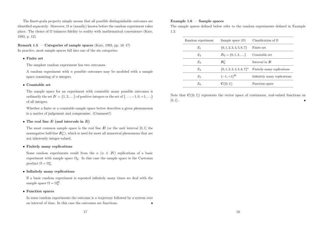
Example 1.6 — Sample spaces
The sample spaces defined below refer to the random experiments defined in Example
1.2:
Random experiment Sample space (!) Classification of !
E1 {0, 1, 2, 3, 4, 5, 6, 7} Finite set
E2 IN0 = {0, 1, 2, . . .} Countable set
E3 IR+0 Interval in IR
E4 {0, 1, 2, 3, 4, 5, 6, 7}n Finitely many replications
E5 {!1,+1}IN Infinitely many replications
E6 C([0, 1]) Function space
Note that C([0, 1]) represents the vector space of continuous, real-valued functions on
[0, 1]. •
18

1.2 Events and classes of sets
Definition 1.7 — Event (Karr, 1993, p. 18)
Given a random experiment with sample space !, an event can be provisionally defined
as a subset of ! whose probability is defined. •
Remark 1.8 — An event A occurs if the outcome ! of the random experiment belongs
to A, i.e. ! " A. •
Example 1.9 — Events
Some events associated to the six random experiments described in examples 1.2 and 1.6:
E.A. Event
E1 A = “observe at least 3 students in the 4th. row”
= {3, . . . , 7}
E2 B = “observe more than 4 car accidents in 12 hours”
= {5, 6, . . .}
E3 C = “wait more than 8 minutes”
= (8,+,)
E4 D = “observe at least 3 students in the 4th. row, in 5 consecutive days”
= {3, . . . , 7}5
E5 E = “an ascending path”
= {(1, 1, . . .)}
E6 F = “temperature above 250o over the interval [0, 1]”
= {f " C([0, 1]) : f(x) > 250, x " [0, 1]}
•
Definition 1.10 — Set operations (Resnick, 1999, p. 3)
As subsets of the sample space !, events can be manipulated using set operations. The
set operations which you should know and will be commonly used are listed next:
• Complementation
The complement of an event A # ! is
Ac = {! " ! : ! &" A}. (1.3)
19
• Intersection
The intersection of events A and B (A, B # !) is
A $B = {! " ! : ! " A and ! " B}. (1.4)
The events A and B are disjoint (mutually exclusive) if A $ B = %, i.e. they have
no outcomes in common, therefore they never happen at the same time.
• Union
The union of events A and B (A, B # !) is
A 0B = {! " ! : ! " A or ! " B}. (1.5)
Karr (1993) uses A + B to denote A 0B when A and B are disjoint.
• Set di!erence
Given two events A and B (A, B # !), the set di"erence between B and A consists
of those outcomes in B but not in A:
B\A = B $ Ac. (1.6)
• Symmetric di!erence
Let A and B be two events (A, B # !). Then the outcomes that are in one but not
in both sets consist on the symmetric di"erence:
A%B = (A\B) 0 (B\A). (1.7)
•
Exercise 1.11 — Set operations
Represent the five set operations in Definition 1.10 pictorially by Venn diagrams. •
Proposition 1.12 — Properties of set operations (Resnick, 1999, pp. 4–5)
Set operations satisfy well known properties such as commutativity, associativity, De
Morgan’s laws, etc., providing now and then connections between set operations. These
properties have been condensed in the following table:
20

Set operation Property
Complementation (Ac)c = A
%c = !!c = %
Intersection and union CommutativityA $B = B $A, A 0B = B 0A
A $ % = %, A 0 % = A
A $A = A, A 0A = A
A $ ! = A, A 0 ! = !A $Ac = %, A 0Ac = !
Associativity(A $B) $ C = A $ (B $ C)(A 0B) 0 C = A 0 (B 0 C)
De Morgan’s laws(A $B)c = Ac 0Bc
(A 0B)c = Ac $Bc
Distributivity(A $B) 0 C = (A 0 C) $ (B 0 C)(A 0B) $ C = (A $ C) 0 (B $ C)
•
Definition 1.13 — Relations between sets (Resnick, 1999, p. 4)
Now we list ways sets A and B can be compared:
• Set containment or inclusion
A is a subset of B, written A # B or B 1 A, i" A $B = A. This means that
! " A . ! " B. (1.8)
So if A occurs then B also occurs. However, the occurrence of B does not imply
the occurrence of A.
• Equality
Two events A and B are equal, written A = B, i" A # B and B # A. This means
! " A 2 ! " B. (1.9)
•
21
Proposition 1.14 — Properties of set containment (Resnick, 1999, p. 4)
These properties are straightforward but we stated them for the sake of completeness and
their utility in the comparison of the probabilities of events:
• A # A
• A # B, B # C . A # C
• A # C, B # C . (A 0B) # C
• A 1 C, B 1 C . (A $B) 1 C
• A # B 2 Bc # Ac. •
These properties will be essential to calculate or relate probabilities of (sophisticated)
events.
Remark 1.15 — The jargon of set theory and probability theory
What follows results from minor changes of Table 1.1 from Grimmett and Stirkazer (2001,
p. 3):
Typical notation Set jargon Probability jargon
! Collection of objects Sample space
! Member of ! Outcome
A Subset of ! Event (that some outcome in A occurs)
Ac Complement of A Event (that no outcome in A occurs)
A $B Intersection A and B occur
A 0B Union Either A or B or both A and B occur
B\A Di"erence B occurs but not A
A#B Symmetric di"erence Either A or B, but not both, occur
A # B Inclusion If A occurs then B occurs too
% Empty set Impossible event
! Whole space Certain event
•
22

Functions on the sample space (such as random variables defined in the next chapter)
are even more important than events themselves.
An indicator function is the simplest way to associate a set with a (binary) function.
Definition 1.16 — Indicator function (Karr, 1993, p. 19)
The indicator function of the event A # ! is the function on ! given by
1A(w) =
71 if w " A
0 if w &" A(1.10)
Therefore, 1A indicates whether A occurs. •
The indicator function of an event, which resulted from a set operation on events A
and B, can often be written in terms of the indicator functions of these two events.
Proposition 1.17 — Properties of indicator functions (Karr, 1993, p. 19)
Simple algebraic operations on the indicator functions of the events A and B translate
set operations on these two events:
1Ac = 1! 1A (1.11)
1A#B = min{1A,1B}= 1A ) 1B (1.12)
1A(B = max{1A,1B}; (1.13)
1B\A = 1B#Ac
= 1B ) (1! 1A) (1.14)
1A!B = |1A ! 1B|. (1.15)
•
Exercise 1.18 — Indicator functions
Solve exercises 1.1 and 1.7 of Karr (1993, p. 40). •
The definition of indicator function quickly yields the following result when we are
able compare events A and B.
23
Proposition 1.19 — Another property of indicator functions (Resnick, 1999, p.
5)
Let A and B be two events of !. Then
A 3 B 2 1A ' 1B. (1.16)
Note here that we use the convention that for two functions f , g with domain ! and range
IR, we have f ' g i" f(!) ' g(!) for all ! " !. •
Motivation 1.20 — Limits of sets (Resnick, 1999, p. 6)
The definition of convergence concepts for random variables rests on manipulations of
sequences of events which require the definition of limits of sets. •
Definition 1.21 — Operations on sequences of sets (Karr, 1993, p. 20)
Let (An)n"IN be a sequence of events of !. Then the union and the intersection of (An)n"IN
are defined as follows
+!#
n=1
An = {! : ! " An for some n} (1.17)
+!8
n=1
An = {! : ! " An for all n}. (1.18)
The sequence (An)n"IN is said to be pairwise disjoint if Ai $ Aj = % whenever i &= j. •
Definition 1.22 — Lim sup, lim inf and limit set (Karr, 1993, p. 20)
Let (An)n"IN be a sequence of events of !. Then we define the two following limit sets:
lim sup An =+!8
k=1
+!#
n=k
An (1.19)
= {! " ! : ! " An for infinitely many values of n}= {An, i.o.}
lim inf An =+!#
k=1
+!8
n=k
An (1.20)
= {! " ! : ! " An for all but finitely many values of n}= {An, ult.},
where i.o. and ult. stand for infinitely often and ultimately, respectively.
24
Let A be an event of !. Then the sequence (An)n"IN is said to converge to A, written
An 4 A or limn&+!An = A, if
lim inf An = lim sup An = A. (1.21)
•
Example 1.23 — Lim sup, lim inf and limit set
Let (An)n"IN be a sequence of events of ! such that
An =
7A for n even
Ac for n odd.(1.22)
Then
lim sup An =+!8
k=1
+!#
n=k
An
= ! (1.23)
&=
lim inf An =+!#
k=1
+!8
n=k
An
= %, (1.24)
so there is no limit set limn&An. •
Exercise 1.24 — Lim sup, lim inf and limit set
Solve Exercise 1.3 of Karr (1993, p. 40). •
Proposition 1.25 — Properties of lim sup and lim inf (Resnick, 1999, pp. 7–8)
Let (An)n"IN be a sequence of events of !. Then
lim inf An # lim sup An (1.25)
(lim inf An)c = lim sup(Acn). (1.26)
•
25
Definition 1.26 — Monotone sequences of events (Resnick, 1999, p. 8)
Let (An)n"IN be a sequence of events of !. It is said to be monotone non-decreasing,
written An 5, if
A1 3 A2 3 A3 3 . . . . (1.27)
(An)n"IN is monotone non-increasing, written An 6, if
A1 7 A2 7 A3 7 . . . . (1.28)
•
Proposition 1.27 — Properties of monotone sequences of events (Karr, 1993,
pp. 20–21)
Suppose (An)n"IN be a monotone sequence of events. Then
An 5 . limn&+!
An =+!#
n=1
An (1.29)
An 6 . limn&+!
An =+!8
n=1
An. (1.30)
•
Exercise 1.28 — Properties of monotone sequences of events
Prove Proposition 1.27. •
Example 1.29 — Monotone sequences of events
The Galton-Watson process is a branching stochastic process arising from Francis Galton’s
statistical investigation of the extinction of family names. Modern applications include the
survival probabilities for a new mutant gene, [...], or the dynamics of disease outbreaks
in their first generations of spread, or the chances of extinction of small populations of
organisms. (http://en.wikipedia.org/wiki/Galton-Watson process)
Let (Xn)IN0 be a stochastic process, where Xn represents the size of generation n. A
(Xn)IN0 is Galton-Watson process if it evolves according to the recurrence formula:
• X0 = 1 (we start with one individual); and
• Xn+1 =!Xn
i=1 Z(n)i , where, for each n, Z(n)
i represents the number of descendants of
the individual i from generation n and9Z(n)
i
:
i"INis a sequence of i.i.d. non-negative
random variables.
26
Let An = {Xn = 0}. Since A1 . A2 . . . ., i.e. (An)n"IN is a non-decreasing monotone
sequence of events, written An 5, we get An 4 A =;+!
n=1 An. Moreover, the extinction
probability is given by
P ({Xn = 0 for some n}) = P
"+!#
n=1
{Xn = 0}$
= P
'lim
n&+!{Xn = 0}
(
= P
"+!#
n=1
An
$
= P
'lim
n&+!An
(. (1.31)
Later on, we shall conclude that we can conveniently interchange the limit sign and
the probability function and add: P (Xn = 0 for some n) = P (limn&+!{Xn = 0}) =
limn&+! P ({Xn = 0}). •
Proposition 1.30 — Limits of indicator functions (Karr, 1993, p. 21)
In terms of indicator functions,
An 4 A 2 1An(w) 4 1A(w), (w " !. (1.32)
Thus, the convergence of sets is the same as pointwise convergence of their indicator
functions. •
Exercise 1.31 — Limits of indicator functions (Exercise 1.8, Karr, 1993, p. 40)
Prove Proposition 1.30. •
Motivation 1.32 — Closure under set operations (Resnick, 1999, p. 12)
We need the notion of closure because we want to combine and manipulate events to make
more complex events via set operations and we require that certain set operations do not
carry events outside the family of events. •
Definition 1.33 — Closure under set operations (Resnick, 1999, p. 12)
Let C be a collection of subsets of !. C is closed under a set operation7 if the set obtained
by performing the set operation on sets in C yields a set in C. •7Be it a countable union, finite union, countable intersection, finite intersection, complementation,
monotone limits, etc.
27
Example 1.34 — Closure under set operations (Resnick, 1999, p. 12)
• C is closed under finite union if for any finite collection A1, . . . , An of sets in C,;n
i=1 Ai " C.
• Suppose ! = IR and C = {finite real intervals} = {(a, b] : !, < a < b < +,}.Then C is not closed under finite unions since (1, 2]0 (36, 37] is not a finite interval.
However, C is closed under intersection since (a, b]$(c, d] = (max{a, c}, min{b, d}] =
(a 8 c, b 9 d].
• Consider now ! = IR and C = {open real subsets}. C is not closed under
complementation since the complement of an open set is not open. •
Definition 1.35 — Algebra (Resnick, 1999, p. 12)
A is an algebra (or field) on ! if it is a non-empty class of subsets of ! closed under finite
union, finite intersection and complementation.
A minimal set of postulates for A to be an algebra on ! is:
1. ! " A
2. A " A. Ac " A
3. A, B " A. A 0B " A. •
Remark 1.36 — Algebra
Please note that, by the De Morgan’s laws, A is closed under finite intersection ((A0B)c =
Ac $Bc " A), thus we do not need a postulate concerning finite intersection. •
Motivation 1.37 — #-algebra (Karr, 1993, p. 21)
To define a probability function dealing with an algebra is not enough: we need to define
a collection of sets which is closed under countable union, countable intersection, and
complementation. •
Definition 1.38 — #!algebra (Resnick, 1999, p. 12)
F is a #!algebra on ! if it is a non-empty class of subsets of ! closed under countable
union, countable intersection and complementation.
A minimal set of postulates for F to be an #!algebra on ! is:
28

1. ! " F
2. A " F . Ac " F
3. A1, A2, . . . " F .;+!
i=1 Ai " F . •
Example 1.39 — #!algebra (Karr, 1993, p. 21)
• Trivial #!algebra
F = {%, !}
• Power set
F = IP (!) = class of all subsets of !
In general, neither of these two #!algebras is specially interesting or useful — we need
something in between. •
Definition 1.40 — Generated #!algebra (http://en.wikipedia.org/wiki/Sigma-
algebra)
If U is an arbitrary family of subsets of ! then we can form a special #!algebra
containing U , called the #!algebra generated by U and denoted by #(U), by intersecting
all #!algebras containing U .
Defined in this way #(U) is the smallest/minimal #!algebra on ! that contains U . •
Example 1.41 — Generated #!algebra (http://en.wikipedia.org/wiki/Sigma-
algebra; Karr, 1993, p. 22)
• Trivial example
Let ! = {1, 2, 3} and U = {{1}}. Then #(U) = {%, {1}, {2, 3}, !} is a #!algebra
on !.
• #!algebra generated by a finite partition
If U = {A1, . . . , An} is a finite partition of ! — that is, A1, . . . , An are disjoint and;n
i=1 Ai = ! — then #(U) = {;
i"I Ai : I 3 {1, . . . , n}} which includes %.
• #!algebra generated by a countable partition
If U = {A1, A2, . . .} is a countable partion of ! — that is, A1, A2, , . . . are disjoint
and;+!
i=1 Ai = ! — then #(U) = {;
i"I Ai : I 3 IN} which also includes %. •
29
Since we tend to deal with real random variables we have to define a #!algebra on
! = IR and the power set on IR, IP (IR) is not an option. The most important #!algebra
on IR is the one defined as follows.
Definition 1.42 — Borel #!algebra on IR (Karr, 1993, p. 22)
The Borel #!algebra on IR, denoted by B(IR), is generated by the class of intervals
U = {(a, b] : !, < a < b < +,}, (1.33)
that is, #(U) = B(IR). Its elements are called Borel sets.8 •
Remark 1.43 — Borel #!algebra on IR (Karr, 1993, p. 22)
• Every “reasonable” set of IR — such as intervals, closed sets, open sets, finite sets,
and countable sets — belong to B(IR). For instance, {x} =<+!
n=1(x! 1/n, x].
• Moreover, the Borel #!algebra on IR, B(IR), can also be generated by the class of
intervals {(!,, a] : !, < a < +,} or {(b, +,) : !, < b < +,}.
• B(IR) &= IP (IR).
• An example of a subset of the reals which is not a Borel set is
due to Lusin (1927, pp. 76–78) and is described in some detail in
http://en.wikipedia.org/wiki/Borel set#Non-Borel sets. •
Definition 1.44 — Borel #!algebra on IRd (Karr, 1993, p. 22)
The Borel #!algebra on IRd, d " IN , B(IRd), is generated by the class of rectangles that
are Cartesian products of real intervals
U =
7d&
i=1
(ai, bi] : !, < ai < bi < +,, i = 1, . . . , d
=. (1.34)
•
Exercise 1.45 — Generated #!algebra (Exercise 1.9, Karr, 1993, p. 40)
Given sets A and B of !, identify all sets in #({A, B}). •
Exercise 1.46 — Borel #!algebra on IR (Exercise 1.10, Karr, 1993, p. 40)
Prove that {x} is a Borel set for every x " IR. •
8Borel sets are named after Emile Borel. Along with Rene-Louis Baire and HenriLebesgue, he was among the pioneers of measure theory and its application to probability theory(http://en.wikipedia.org/wiki/Emile Borel).
30

1.3 Probabilities and probability functions
Motivation 1.47 — Probability function (Karr, 1993, p. 23)
A probability is a set function, defined for events; it should be countably additive (i.e.
#!additive), that is, the probability of a countable union of disjoint events is the sum of
their individual probabilities. •
Definition 1.48 — Probability function (Karr, 1993, p. 24)
Let ! be the sample space and F be the #!algebra of events of !. A probability on
(!,F) is a function P : ! 4 IR such that:
1. Axiom 1 9 — P (A) - 0, (A " F .
2. Axiom 2 — P (!) = 1.
3. Axiom 3 (countable additivity or #!additivity)
Whenever A1, A2, . . . are (pairwise) disjoint events in F ,
P
"+!#
i=1
Ai
$=
+!%
i=1
P (Ai). (1.35)
•
Remark 1.49 — Probability function
The probability function P transforms events in real numbers in [0, 1]. •
Definition 1.50 — Probability space (Karr, 1993, p. 24)
The triple (!,F , P ) is a probability space. •
Example 1.51 — Probability function (Karr, 1993, p. 25)
Let
• {A1, . . . , An} be a finite partition of ! — that is, A1, . . . , An are (nonempty and
pairwise) disjoint events and;n
i=1 Ai = !;
• F be the #!algebra generated by the finite partition {A1, A2, . . . , An}, i.e. F =
#({A1, . . . , An});
• p1, . . . , pn positive numbers such that!n
i=1 pi = 1.
9Righter (200—) called the first and second axioms duh rules.
31
Then the function defined as
P
"#
i"I
Ai
$=
%
i"I
pi, (I 3 {1, . . . , n}, (1.36)
where pi = P (Ai), is a probability function on (!,F). •
Exercise 1.52 — Probability function (Exercise 1.11, Karr, 1993, p. 40)
Let A, B and C be disjoint events such that: A 0 B 0 C = !; P (A) = 0.6, P (B) = 0.3
and P (C) = 0.1. Calculate all probabilities of all events in #({A, B, C}). •
Motivation 1.53 — Elementary properties of probability functions
The axioms do not teach us how to calculate the probabilities of events. However, they
establish rules for their calculation such as the following ones. •
Proposition 1.54 — Elementary properties of probability functions (Karr, 1993,
p. 25)
Let (!,F , P ) be a probability space then:
1. Probability of the empty set
P (%) = 0. (1.37)
2. Finite additivity
If A1, . . . , An are (pairwise) disjoint events then
P
"n#
i=1
Ai
$=
n%
i=1
P (Ai). (1.38)
Probability of the complement of A
Consequently, for each A,
P (Ac) = 1! P (A). (1.39)
3. Monotonicity of the probability function
If A 3 B then
P (B \ A) = P (B)! P (A). (1.40)
Therefore if A 3 B then
P (A) ' P (B). (1.41)
32
4. Addition rule
For all A and B (disjoint or not),
P (A 0B) = P (A) + P (B)! P (A $B). (1.42)
•
Remark 1.55 — Elementary properties of probability functions
According to Righter (200—), (1.41) is another duh rule but adds one of Kahneman and
Tversky’s most famous examples, the Linda problem.
Subjects were told the story (in the 70’s):
• Linda is 31 years old, single, outspoken, and very bright. She majored in philosophy.
As a student she was deeply concerned with issues of discrimination and social justice
and also participated in anti nuclear demonstrations.
They are asked to rank the following statements by their probabilities:
• Linda is a bank teller.
• Linda is a bank teller who is active in the feminist movement.
Kahneman and Tversky found that about 85% of the subjects ranked “Linda is a bank
teller and is active in the feminist movement” as more probable than “Linda is a bank
teller”. •
Exercise 1.56 — Elementary properties of probability functions
Prove properties 1. through 4. of Proposition 1.54 and that
P (B \ A) = P (B)! P (A $B) (1.43)
P (A%B) = P (A 0B)! P (A $B) = P (A) + P (B)! 2) P (A $B). (1.44)
Hints (Karr, 1993, p. 25):
• property 1. can be also proved by using the finite additivity;
• property 2. by considering An+1 = An+2 = . . . = %;
• property 3. by rewriting B as (B \ A) 0 (A $B) = (B \ A) 0 A;
• property 4. by rewriting A 0B as (A \B) 0 (A $B) 0 (B \ A). •
33
We proceed with some advanced properties of probability functions.
Proposition 1.57 — Boole’s inequality or #!subadditivity (Karr, 1993, p. 26)
Let A1, A2, . . . be events in F . Then
P
"+!#
n=1
An
$'
+!%
n=1
P (An). (1.45)
•
Exercise 1.58 — Boole’s inequality or #!subadditivity
Prove Boole’s inequality by using the disjointification technique (Karr, 1993, p. 26),10 the
fact that Bn = An \-;n$1
i=1 Ai
.3 An, and by applying the #!additivity and monotonicity
of probability functions. •
Proposition 1.59 — Finite subadditivity (Resnick, 1999, p. 31)
The probability function P is finite subadditive in the sense that
P
"n#
i=1
Ai
$'
n%
i=1
P (Ai), (1.46)
for all events A1, . . . , An. •
Remark 1.60 — Finite additivity
Finite additivity is a consequence of Boole’s inequality (i.e. #!subadditivity). However,
finite additivity does not imply #!subadditivity. •
Proposition 1.61 — Inclusion-exclusion formula (Resnick, 1999, p. 30)
If A1, . . . , An are events, then the probability of their union can be written as follows:
P
"n#
i=1
Ai
$=
n%
i=1
P (Ai)!%
1'i<j'n
P (Ai $ Aj) +%
1'i<j<k'n
P (Ai $ Aj $ Ak)
! . . .! (!1)n ) P (A1 $ . . . $ An). (1.47)
•
Remark 1.62 — Inclusion-exclusion formula
• The terms on the right side of (1.47) alternate in sign and give inequalities called
Bonferroni inequalities11 when we neglect the remainders. Two examples:
10Note that;+"
n=1 An =;+"
n=1 Bn, where Bn = An \9;n!1
i=1 Ai
:are disjoint events.
11They are named after Italian mathematician Carlo Emilio Bonferroni.
34
P
"n#
i=1
Ai
$'
n%
i=1
P (Ai) (1.48)
P
"n#
i=1
Ai
$-
n%
i=1
P (Ai)!%
1'i<j'n
P (Ai $ Aj) (1.49)
(Resnick, 1999, p. 30).
• Let the event Ai represent the rejection of the (simple) null hypothesis H0,i
(i = 1, . . . , n). Then if we test the (multiple or simultaneous) null hypothesis
H0 : $ni=1H0,i, the probability of rejecting H0 is equal to the probability of rejecting
at least one of the (simple) null hypotheses. Moreover, this probability does not
exceed the sum of the probabilities of individually rejecting each of the (simple)
null hypotheses:
P
"n#
i=1
Ai
$'
n%
i=1
P (Ai).
Consequently, if the desired significance level for the test involving H0 is set
to be equal to $0, then the Bonferroni correction leads to the conclusion that
each individual null hypothesis should be tested at a significance level of $0/n
(http://en.wikipedia.org/wiki/Bonferroni correction). •
Exercise 1.63 — Inclusion-exclusion formula
Prove the inclusion-exclusion formula by induction using the addition rule for n = 2
(Resnick, 1999, p. 30). •
Proposition 1.64 — Monotone continuity (Resnick, 1999, p. 31)
Probability functions are continuous for monotone sequences of events in the sense that:
1. If An 5 A, where An " F , then P (An) 5 P (A).
2. If An 6 A, where An " F , then P (An) 6 P (A). •
Exercise 1.65 — Monotone continuity
Prove Proposition 1.64 by using the disjointification technique, the monotone character
of the sequence of events and #!additivity (Resnick, 1999, p. 31).
For instance property 1. can be proved as follows.
• A1 # A2 # A3 # . . . # An # . . .;
35
• B1 = A1, B2 = A2 \A1, B3 = A3 \ (A1 0A2), . . . , Bn = An \-;n$1
i=1 Ai
.are disjoint
events;
• since A1, A2, . . . is a non-decreasing sequence of events An 5 A =;+!
n=1 An =;+!
n=1 Bn, Bn = An \ An$1, and;n
i=1 Bi = An; if we add to this #!additivity,
we conclude that
P (A) = P
"+!#
n=1
An
$= P
"+!#
n=1
Bn
$=
+!%
n=1
P (Bn)
= limn&+!
5n%
i=1
P (Bi) = limn&+!
5 P
"n#
i=1
Bi
$= lim
n&+!5 P (An).
•
Motivation 1.66 — #!additivity as a result of finite additivity and monotone
continuity (Karr, 1993, p. 26)
The next theorem shows that # ! additivity is equivalent to the confluence of finite
additivity (which is reasonable) and monotone continuity (which is convenient and
desirable mathematically). •
Theorem 1.67 — #!additivity as a result of finite additivity and monotone
continuity (Karr, 1993, p. 26)
Let P be a nonnegative, finitely additive set function on F with P (!) = 1. Then, the
following are equivalent:
1. P is #!additive (thus a probability function).
2. Whenever An 5 A in F , P (An) 5 P (A).
3. Whenever An 6 A in F , P (An) 6 P (A).
4. Whenever An 6 % in F , P (An) 6 0. •
Exercise 1.68 — #!additivity as a result of finite additivity and monotone
continuity
Prove Theorem 1.67.
Note that we need to prove 1. . 2. . 3. . 4. . 1. But since 2. 2 3. by
complementation and 4. is a special case of 3. we just need to prove that 1. . 2. and
4. . 1. (Karr, 1993, pp. 26-27). •
36

Remark 1.69 — Inf, sup, lim inf and lim sup
Let a1, a2, . . . be a sequence of real numbers. Then
• Infimum
The infimum of the set {a1, a2, . . .} — written inf an — corresponds to the greatest
element (not necessarily in {a1, a2, . . .}) that is less than or equal to all elements of
{a1, a2, . . .}.12
• Supremum
The supremum of the set {a1, a2, . . .} — written sup an — corresponds to the
smallest element (not necessarily in {a1, a2, . . .}) that is greater than or equal to
every element of {a1, a2, . . .}.13
• Limit inferior and limit superior of a sequence of real numbers 14
lim inf an = supk)1 infn)k an
lim sup an = infk)1 supn)k an.
Let A1, A2, . . . be a sequence of events. Then
• Limit inferior and limit superior of a sequence of sets
lim inf An =;+!
k=1
<+!n=k An
lim sup An =<+!
k=1
;+!n=k An. •
Motivation 1.70 — A special case of the Fatou’s lemma
This result plays a vital role in the proof of continuity of probability functions. •
Proposition 1.71 — A special case of the Fatou’s lemma (Resnick, 1999, p. 32)
Suppose A1, A2, . . . is a sequence of events in F . Then
P (lim inf An) ' lim inf P (An) ' lim sup P (An) ' P (lim sup An). (1.50)
•
Exercise 1.72 — A special case of the Fatou’s lemma
Prove Proposition 1.71 (Resnick, 1999, pp. 32-33; Karr, 1993, p. 27). •12For more details check http://en.wikipedia.org/wiki/Infimum13http://en.wikipedia.org/wiki/Supremum14http://en.wikipedia.org/wiki/Limit superior and limit inferior
37
Theorem 1.73 — Continuity (Karr, 1993, p. 27)
If An 4 A then P (An) 4 P (A). •
Exercise 1.74 — Continuity
Prove Theorem 1.73 by using Proposition 1.71 (Karr, 1993, p. 27). •
Motivation 1.75 — (1st.) Borel-Cantelli Lemma (Resnick, 1999, p. 102)
This result is simple but still is a basic tool for proving almost sure convergence of
sequences of random variables (see Chapter 5). •
Theorem 1.76 — (1st.) Borel-Cantelli Lemma (Resnick, 1999, p. 102; Karr, 1993,
p. 27)
Let A1, A2, . . . be any events in F . Then
+!%
n=1
P (An) < +, . P (lim sup An) = 0. (1.51)
•
Exercise 1.77 — (1st.) Borel-Cantelli Lemma
Prove Theorem 1.76 (Resnick, 1999, p. 102; Karr, 1993, p. 27). •
38

1.4 Distribution functions; discrete, absolutely
continuous and mixed probabilities
Motivation 1.78 — Distribution function (Karr, 1993, pp. 28-29)
A probability function P on the Borel #!algebra B(IR) is determined by its values
P ((!,, x]), for all intervals (!,, x].
Probability functions on the real line play an important role as distribution functions
of random variables. •
Definition 1.79 — Distribution function (Karr, 1993, p. 29)
Let P be a probability function defined on (IR,B(IR)). The distribution function
associated to P is represented by FP and defined by
FP (x) = P ((!,, x]), x " IR. (1.52)
•
Theorem 1.80 — Some properties of distribution functions (Karr, 1993, pp. 29-
30)
Let FP be the distribution function associated to P . Then
1. FP is non-decreasing. Hence, the left-hand limit
FP (x$) = lims*x, s<x
FP (s) (1.53)
and the right-hand limit
FP (x+) = lims+x, s>x
FP (s) (1.54)
exist for each x, and
FP (x$) ' FP (x) ' FP (x+). (1.55)
2. FP is right-continuous, i.e.
FP (x+) = FP (x) (1.56)
for each x.
3. FP has the following limits:
limx&$!
FP (x) = 0 (1.57)
limx&+!
FP (x) = 1. (1.58)
•
39
Definition 1.81 — Distribution function (Resnick, 1999, p. 33)
A function FP : IR 4 [0, 1] satisfying properties 1., 2. and 3. from Theorem 1.80 is called
a distribution function. •
Exercise 1.82 — Some properties of distribution functions
Prove Theorem 1.80 (Karr, 1993, p. 30). •
Definition 1.83 — Survival (or survivor) function (Karr, 1993, p. 31)
The survival (or survivor) function associated to P is
SP (x) = 1! FP (x) = P ((x, +,)), x " IR. (1.59)
SP (x) are also termed tail probabilities. •
Proposition 1.84 — Probabilities in terms of the distribution function (Karr,
1993, p. 30)
The following table condenses the probabilities of various intervals in terms of the
distribution function
Interval I Probability P (I)
(!,, x] FP (x)
(x,+,) 1! FP (x)
(!,, x) FP (x$)
[x,+,) 1! FP (x$)
(a, b] FP (b)! FP (a)
[a, b) FP (b$)! FP (a$)
[a, b] FP (b)! FP (a$)
(a, b) FP (b$)! FP (a)
{x} FP (x)! FP (x$)
where x " IR and !, < a < b < +,. •
Example 1.85 — Point mass (Karr, 1993, p. 31)
Let P be defined as
P (A) = %s(A) =
71, if s " A
0, otherwise,(1.60)
for every event A " F , i.e. P is a point mass at s. Then
40

FP (x) = P ((!,, x])
=
70, x < s
1, x - s.(1.61)
The property that FP (x) only takes values 0 or 1 characterizes point masses. •
Example 1.86 — Uniform distribution on [0, 1] (Karr, 1993, p. 31)
Let P be defined as
P ((a, b]) = Length((a, b] $ [0, 1]), (1.62)
for any real interval (a, b] with !, < a < b < +,. Then
FP (x) = P ((!,, x])
=
)*+
*,
0, x < 0
x, 0 ' x ' 1
1, x > 1.
(1.63)
•
We are going to revisit the discrete and absolutely continuous probabilities and
introduce mixed distributions.
Definition 1.87 — Discrete probabilities (Karr, 1993, p. 32)
A probability function P defined on (IR,B(IR)) is said to be discrete if there is a countable
set C such that P (C) = 1. •
Remark 1.88 — Discrete probabilities (Karr, 1993, p. 32)
Discrete probabilities are finite or countable convex combinations of point masses. The
associated distribution functions do not increase “smoothly” — they increase only by
means of jumps. •
Proposition 1.89 — Discrete probabilities (Karr, 1993, p. 32)
Let P be a probability function on (IR,B(IR)). Then the following are equivalent:
1. P is a discrete probability.
2. There is a real sequence x1, x2, . . . and numbers p1, p2, . . . with pn > 0, for all n, and!+!
n=1 pn = 1 such that
P (A) =+!%
n=1
pn ) %xn(A), (1.64)
for all A " B(IR).
41
3. There is a real sequence x1, x2, . . . and numbers p1, p2, . . . with pn > 0, for all n, and!+!
n=1 pn = 1 such that
FP (x) =+!%
n=1
pn ) 1[xn,+!)(x), (1.65)
for all x " IR. •
Remark 1.90 — Discrete probabilities (Karr, 1993, p. 33)
The distribution function associated to a discrete probability increases only by jumps of
size pn at xn. •
Exercise 1.91 — Discrete probabilities
Prove Proposition 1.89 (Karr, 1993, p. 32). •
Example 1.92 — Discrete probabilities
Let px represent from now on P ({x}).
• Uniform distribution on a finite set C
px = 1#C , x " C
P (A) = #A#C , A 3 C.
This distribution is also known as the Laplace distribution.
• Bernoulli distribution with parameter p (p " [0, 1])
C = {0, 1}
px = px(1! p)1$x, x " C.
This probability function arises in what we call a Bernoulli trial — a yes/no random
experiment which yields success with probability p.
• Binomial distribution with parameters n and p (n " IN, p " [0, 1])
C = {0, 1, . . . , n}
px =-
nx
.px(1! p)n$x, x " C.
The binomial distribution is the discrete probability distribution of the number of
successes in a sequence of n independent yes/no experiments, each of which yields
success with probability p.
Moreover, the result!n
x=0 px = 1 follows from the binomial theorem
(http://en.wikipedia.org/wiki/Binomial theorem).
42
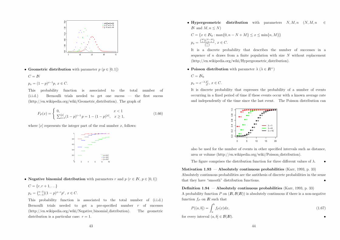
• Geometric distribution with parameter p (p " [0, 1])
C = IN
px = (1! p)x$1p, x " C.
This probability function is associated to the total number of
(i.i.d.) Bernoulli trials needed to get one sucess — the first sucess
(http://en.wikipedia.org/wiki/Geometric distribution). The graph of
FP (x) =
70, x < 1![x]
i=1(1! p)i$1 p = 1! (1! p)[x], x - 1,(1.66)
where [x] represents the integer part of the real number x, follows:
• Negative binomial distribution with parameters r and p (r " IN, p " [0, 1])
C = {r, r + 1, . . .}
px =-
x$1r$1
.(1! p)x$rpr, x " C.
This probability function is associated to the total number of (i.i.d.)
Bernoulli trials needed to get a pre-specified number r of sucesses
(http://en.wikipedia.org/wiki/Negative binomial distribution). The geometric
distribution is a particular case: r = 1.
43
• Hypergeometric distribution with parameters N, M, n (N, M, n "IN and M, n ' N)
C = {x " IN0 : max{0, n!N + M} ' x ' min{n, M}}
px =(M
x )(N!Mn!x )
(Nn)
, x " C.
It is a discrete probability that describes the number of successes in a
sequence of n draws from a finite population with size N without replacement
(http://en.wikipedia.org/wiki/Hypergeometric distribution).
• Poisson distribution with parameter & (& " IR+)
C = IN0
px = e$" "x
x! , x " C.
It is discrete probability that expresses the probability of a number of events
occurring in a fixed period of time if these events occur with a known average rate
and independently of the time since the last event. The Poisson distribution can
also be used for the number of events in other specified intervals such as distance,
area or volume (http://en.wikipedia.org/wiki/Poisson distribution).
The figure comprises the distribution function for three di"erent values of &. •
Motivation 1.93 — Absolutely continuous probabilities (Karr, 1993, p. 33)
Absolutely continuous probabilities are the antithesis of discrete probabilities in the sense
that they have “smooth” distribution functions. •
Definition 1.94 — Absolutely continuous probabilities (Karr, 1993, p. 33)
A probability function P on (IR,B(IR)) is absolutely continuous if there is a non-negative
function fP on IR such that
P ((a, b]) =
6 b
a
fP (x)dx, (1.67)
for every interval (a, b] " B(IR). •
44

Remark 1.95 — Absolutely continuous probabilities
If P is an absolutely continuous probability then FP (x) is an absolutely continuous real
function. •
Remark 1.96 — Continuous, uniformly continuous and absolutely continuous
functions
• Continuous function
A real function f is continuous in x if for any sequence {x1, x2, . . .} such that
limn&! xn = x, it holds that limn&! f(xn) = f(x).
One can say, briefly, that a function is continuous i" it preserves limits.
For the Cauchy definition (epsilon-delta) of continuous function see
http://en.wikipedia.org/wiki/Continuous function
• Uniformly continuous function
Given metric spaces (X, d1) and (Y, d2), a function f : X 4 Y is called uniformly
continuous on X if for every real number % > 0 there exists ' > 0 such that for
every x, y " X with d1(x, y) < ', we have that d2(f(x), f(y)) < %.
If X and Y are subsets of the real numbers, d1 and d2 can be the standard Euclidean
norm, |.|, yielding the definition: for all % > 0 there exists a ' > 0 such that for all
x, y " X, |x! y| < ' implies |f(x)! f(y)| < %.
The di"erence between being uniformly continuous, and simply being continuous at
every point, is that in uniform continuity the value of ' depends only on % and not
on the point in the domain (http://en.wikipedia.org/wiki/Uniform continuity).
• Absolutely continuous function
Let (X, d) be a metric space and let I be an interval in the real line IR. A function f :
I 4 X is absolutely continuous on I if for every positive number %, there is a positive
number ' such that whenever a (finite or infinite) sequence of pairwise disjoint sub-
intervals [xk, yk] of I satisfies!
k |yk ! xk| < ' then!
k d (f(yk), f(xk)) < %.
Absolute continuity is a smoothness property which is stricter than continuity and
uniform continuity.
The two following functions are continuous everywhere but not absolutely
continuous:
1. f(x) = x2 on an unbounded interval;
45
2. f(x) =
70, if x = 0
x sin(1/x), if x &= 0,
on a finite interval containing the origin.
(http://en.wikipedia.org/wiki/Absolute continuity) •
Proposition 1.97 — Absolutely continuous probabilities (Karr, 1993, p. 34)
A probability function P is absolutely continuous i" there is a non-negative function f
on IR such that6 +!
$!f(s)ds = 1 (1.68)
FP (x) =
6 x
$!f(s)ds, x " IR. (1.69)
•
Exercise 1.98 — Absolutely continuous probabilities
Prove Proposition 1.97 (Karr, 1993, p. 34). •
Example 1.99 — Absolutely continuous probabilities
• Uniform distribution on [a, b] (a, b " IR, a < b)
fP (x) =
71
b$a , a ' x ' b
0, otherwise.
FP (x) =
)*+
*,
0, x < ax$ab$a , a ' x ' b
1, x > b.
This absolutely continuous probability is such that all intervals of the same length
on the distribution’s support are equally probable. The support is defined
by the two parameters, a and b, which are its minimum and maximum values
(http://en.wikipedia.org/wiki/Uniform distribution (continuous)).
46

• Exponential distribution with parameter & (& " IR+)
fP (x) =
7&e$"x, x - 0
0, otherwise.
FP (x) =
70, x < 0
1! e$"x, x - 0.
The exponential distribution is used to describe the
times between consecutive events in a Poisson process.15
(http://en.wikipedia.org/wiki/Exponential distribution).
Let P , be the (discrete) Poisson probability with parameter & x. Then
P ,({0}) = e$" x = P ((x, +,)) = 1! FP (x).
• Normal distribution with parameters µ (µ " IR) and #2 (#2 " IR+)
fP (x) = 1%2!#2
exp>! (x$µ)2
2#2
?, x " IR
15I.e. a process in which events occur continuously and independently at a constant average rate.
47
FP (x) =@ x
$! fP (s)ds, x " IR
The normal distribution or Gaussian distribution is used describes data that cluster
around a mean or average. The graph of the associated probability density function
is bell-shaped, with a peak at the mean, and is known as the Gaussian function or
bell curve http://en.wikipedia.org/wiki/Normal distribution). •
Motivation 1.100 — Mixed distributions (Karr, 1993, p. 34)
A probability function need not to be discrete or absolutely continuous... •
Definition 1.101 — Mixed distributions (Karr, 1993, p. 34)
A probability function P is mixed if there is a discrete probability Pd, an absolutely
continuous probability Pc and $ " (0, 1) such that P is a convex combination of Pd and
Pc, that is,
P = $Pd + (1! $)Pc. (1.70)
•
48

Example 1.102 — Mixed distributions
Let M(&)/M(µ)/1 represent a queueing system with Poisson arrivals (rate & > 0) and
exponential service times (rate µ > 0) and one server.
In the equilibrium state, the probability function associated to the waiting time of an
arriving customer is
P (A) = (1! ()%{0}(A) + (PExp(µ(1$$))(A), A " B(IR), (1.71)
where 0 < ( = "µ < 1 and
PExp(µ(1$$))(A) =
6
A
µ(1! () e$µ(1$$) sds. (1.72)
The associated distribution function is given by
FP (x) =
70, x < 0
(1! () + (/1! e$µ(1$$) x
0, x - 0.
(1.73)
•
49
1.5 Conditional probability
Motivation 1.103 — Conditional probability (Karr, 1993, p. 35)
We shall revise probabilities to account for the knowledge that an event has occurred,
using a concept known as conditional probability. •
Definition 1.104 — Conditional probability (Karr, 1993, p. 35)
Let A and B be events. If P (A) > 0 the conditionally probability of B given A is equal to
P (B|A) =P (B $ A)
P (A). (1.74)
In case P (A) = 0, we make the convention that P (B|A) = P (B). •
Remark 1.105 — Conditional probability (Karr, 1993, p. 35)
P (B|A) can be interpreted as the relative likelihood that B occurs given that A is known
to have occured. •
Exercise 1.106 — Conditional probability
Solve exercises 1.23 and 1.24 of Karr (1993, p. 40). •
Example 1.107 — Conditional probability (Grimmett and Stirzaker, 2001, p. 9)
A family has two children.
• What is the probability that both are boys, given that at least one is a boy?
The older and younger child may each be male or female, so there are four possible
combination of sexes, which we assume to be equally likely. Therefore
• ! = {GG, GB, BG, BB}
where G = girl, B = boy, and P (GG) = P (GB) = P (BG) = P (BB) = 14 .
From the definition of conditional probability
P (BB|one boy at least) = P [BB|(GB 0BG 0BB)]
=P [BB $ (GB 0BG 0BB)]
P (GB 0BG 0BB)
=P (BB)
P (GB) + P (BG) + P (BB)
=14
14 + 1
4 + 14
=1
3. (1.75)
A popular but incorrect answer to this question is 12 .
50

This is the correct answer to another question:
• For a family with two children, what is the probability that both are boys given
that the younger is a boy?
In this case
P (BB|younger child is a boy) = P [BB|(GB 0BB)]
= . . .
=P (BB)
P (GB) + P (BB)
=14
14 + 1
4
=1
2. (1.76)
•
Exercise 1.108 — Conditional probability (Grimmett and Stirzaker, 2001, p. 9)
The prosecutor’s fallacy16 — Let G be the event that an accused is guilty, and T the event
that some testimony is true.
Some lawyers have argued on the assumption that P (G|T ) = P (T |G). Show that this
holds i" P (G) = P (T ). •
Motivation 1.109 — Multiplication rule (Montgomery and Runger, 2003, p. 42)
The definition of conditional probability can be rewritten to provide a general expression
for the probability of the intersection of (two) events. This formula is referred to as a
multiplication rule for probabilities. •
Proposition 1.110 — Multiplication rule (Montgomery and Runger, 2003, p. 43)
Let A and B be two events. Then
P (A $B) = P (B|A)) P (A) = P (A|B)) P (B). (1.77)
More generally: let A1, . . . , An be events then
P (A1 $ A2 $ . . . $ An$1 $ An) = P (A1)) P (A2|A1)) P [A3|(A1 $ A2)]
. . .) P [An|(A1 $ A2 $ . . . An$1)]. (1.78)
•16The prosecution made this error in the famous Dreyfus a"air
(http://en.wikipedia.org/wiki/Alfred Dreyfus) in 1894.
51
Example 1.111 — Multiplication rule (Montgomery and Runger, 2003, p. 43)
The probability that an automobile battery, subject to high engine compartment
temperature, su"ers low charging current is 0.7. The probability that a battery is subject
to high engine compartment temperature 0.05.
What is the probability that a battery su"ers low charging current and is subject to
high engine compartment temperature?
• Table of events and probabilities
Event Probability
C = battery su"ers low charging current P (C) =?
T = battery subject to high engine compartment temperature P (T ) = 0.05
C|T = battery su"ers low charging current given that it is P (C|T ) = 0.7
subject to high engine compartment temperature
• Probability
P (C $ T )mult. rule
= P (C|T )) P (T )
= 0.7) 0.05
= 0.035. (1.79)
•
Motivation 1.112 — Law of total probability (Karr, 1993, p. 35)
The next law expresses the probability of an event in terms of its conditional probabilities
given elements of a partition of !. •
Proposition 1.113 — Law of total probability (Karr, 1993, p. 35)
Let {A1, A2, . . .} a countable partition of !. Then, for each event B,
P (B) =+!%
i=1
P (B|Ai)) P (Ai). (1.80)
•
Exercise 1.114 — Law of total probability
Prove Proposition 1.113 by using #!additivity of a probability function and the fact that
B =;+!
i=1 (B $ Ai) (Karr, 1993, p. 36). •
52

Corollary 1.115 — Law of total probability (Montgomery and Runger, 2003, p. 44)
For any events A and B,
P (B) = P (B|A)) P (A) + P (B|Ac)) P (Ac). (1.81)
•
Example 1.116 — Law of total probability (Grimmett and Stirzaker, 2001, p. 11)
Only two factories manufacture zoggles. 20% of the zoggles from factory I and 5% from
factory II are defective. Factory I produces twice as many zoggles as factory II each week.
What is the probability that a zoggle, randomly chosen from a week’s production, is
not defective?
• Table of events and probabilities
Event Probability
D = defective zoggle P (D) =?
A = zoggle made in factory I P (A) = 2) [1! P (A)] = 23
Ac = zoggle made in factory II P (Ac) = 1! P (A) = 13
D|A = defective zoggle given that it is made in factory I P (D|A) = 0.20
D|Ac = defective zoggle given that it is made in factory II P (D|Ac) = 0.05
• Probability
P (Dc) = 1! P (D)lawtotalprob
= 1! [P (D|A)) P (A) + P (D|Ac)) P (Ac)]
= 1!'
0.20) 2
3+ 0.05) 1
3
(
=51
60.
•
Motivation 1.117 — Bayes’ theorem (Karr, 1993, p. 36)
Traditionally (and probably incorrectly) attributed to the English cleric Thomas Bayes
(http://en.wikipedia.org/wiki/Thomas Bayes), the theorem that bears his name is used
to compute conditional probabilities “the other way around”. •
53
Proposition 1.118 — Bayes’ theorem (Karr, 1993, p. 36)
Let {A1, A2, . . .} be a countable partition of !. Then, for each event B with P (B) > 0
and each n,
P (An|B) =P (B|An)P (An)
P (B)
=P (B|An)P (An)
!+!i=1 P (B|Ai)P (Ai)
(1.82)
•
Exercise 1.119 — Bayes’ theorem (Karr, 1993, p. 36)
Prove Bayes’ theorem by using the definition of conditional probability and the law of
total probability (Karr, 1993, p. 36). •
Example 1.120 — Bayes’ theorem (Grimmett and Stirzaker, 2003, p. 11)
Resume Example 1.116...
If the chosen zoggle is defective, what is the probability that it came from factory II.
• Probability
P (A|D) =P (D|A)) P (A)
P (D)
=0.20) 2
3
1! 5160
=8
9. (1.83)
•
54
References
• Grimmett, G.R. and Stirzaker, D.R. (2001). Probability and Random Processes (3rd.
edition). Oxford. (QA274.12-.76.GRI.30385 and QA274.12-.76.GRI.40695 refer to
the library code of the 1st. and 2nd. editions from 1982 and 1992, respectively.)
• Karr, A.F. (1993). Probability. Springer-Verlag.
• Lusin, N. (1927). Sur les ensembles analytiques. Fundamenta Mathematicae 10,
1–95.
• Montgomery, D.C. and Runger, G.C. (2003). Applied statistics and probability for
engineers. John Wiley & Sons, New York. (QA273-280/3.MON.64193)
• Papoulis, A. (1965). Probability, Random Variables and Stochastic Processes.
McGraw-Hill Kogakusha, Ltd. (QA274.12-.76.PAP.28598)
• Resnick, S.I. (1999). A Probability Path. Birkhauser. (QA273.4-.67.RES.49925)
• Righter, R. (200–). Lectures notes for the course Probability and Risk Analysis
for Engineers. Department of Industrial Engineering and Operations Research,
University of California at Berkeley.
• Yates, R.D. and Goodman, D.J. (1999). Probability and Stochastic Processes: A
friendly Introduction for Electrical and Computer Engineers. John Wiley & Sons,
Inc. (QA273-280/4.YAT.49920)
55
Chapter 2
Random variables
2.1 Fundamentals
Motivation 2.1 — Inverse image of sets (Karr, 1993, p. 43)
Before we introduce the concept of random variable (r.v.) we have to talk rather
extensively on inverse images of sets and inverse image mapping. •
Definition 2.2 — Inverse image (Karr, 1993, p. 43)
Let:
• X be a function with domain ! and range !-, i.e. X : ! 4 !-;
• F and F - be the # ! algebras on ! and !-, respectively.
(Frequently !- = IR and F - = B(IR).) Then the inverse image under X of the set B " F -
is the subset of ! given by
X$1(B) = {! : X(!) " B}, (2.1)
written from now on {X " B} (graph!).
•
Remark 2.3 — Inverse image mapping (Karr, 1993, p. 43)
The inverse image mapping X$1 maps subsets of !- to subsets of !. X$1 preserves all
set operations, as well as disjointness. •
56

Proposition 2.4 — Properties of inverse image mapping (Karr, 1993, p. 43;
Resnick, 1999, p. 72)
Let:
• X : ! 4 !-;
• F and F - be the # ! algebras on ! and !-, respectively;
• B, B- and {Bi : i " I} be sets in F -.
Then:
1. X$1(%) = %
2. X$1(!-) = !
3. B 3 B- . X$1(B) 3 X$1(B-)
4. X$1(;
i"I Bi) =;
i"I X$1(Bi)
5. X$1(<
i"I Bi) =<
i"I X$1(Bi)
6. B $B- = % . X$1(B) $X$1(B-) = %
7. X$1(Bc) = [X$1(B)]c. •
Exercise 2.5 — Properties of inverse image mapping
Prove Proposition 2.4 (Karr, 1993, p. 43). •
Proposition 2.6 — # ! algebras and inverse image mapping (Resnick, 1999, pp.
72–73)
Let X : ! 4 !- be a mapping with inverse image. If F - is a # ! algebra on !- then
X$1(F -) = {X$1(B) : B " F -} (2.2)
is a # ! algebra on !.
Exercise 2.7 — # ! algebras and inverse image mapping
Prove Proposition 2.6 by verifying the 3 postulates for a # ! algebra (Resnick, 1999, p.
73). •
57
Proposition 2.8 — Inverse images of # ! algebras generated by classes of
subsets (Resnick, 1999, p. 73)
Let C - be a class of subsets of !-. Then
X$1(#(C -)) = #({X$1(C -)}), (2.3)
i.e., the inverse image of the # ! algebra generated by C - is the same as the # ! algebra
on ! generated by the inverse images. •
Exercise 2.9 — Inverse images of # ! algebras generated by classes of subsets
Prove Proposition 2.8. This proof comprises the verification of the 3 postulates for a
# ! algebra (Resnick, 1999, pp. 73–74) and much more. •
Definition 2.10 — Measurable space (Resnick, 1999, p. 74)
The pair (!,F) consisting of a set ! and a # ! algebra on ! is called a measurable
space. •
Definition 2.11 — Measurable map (Resnick, 1999, p. 74)
Let (!,F) and (!-,F -) be two measurable spaces. Then a map X : ! 4 !- is called a
measurable map if
X$1(F -) 3 F . (2.4)
•
Remark 2.12 — Measurable maps/ Random variables (Karr, 1993, p. 44)
A special case occurs when (!-,F -) = (IR,B(IR)) — in this case X is called a random
variable. That is, random variables are functions on the sample space ! for which inverse
images of Borel sets are events of !. •
Definition 2.13 — Random variable (Karr, 1993, p. 44)
Let (!,F) and (!-,F -) = (IR,B(IR)) be two measurable spaces. A random variable (r.v.)
is a function X : ! 4 IR such that
X$1(B) " F , (B " B(IR). (2.5)
•
58

Remark 2.14 — Random variables (Karr, 1993, p. 44)
A r.v. is a function on the sample space: it transforms events into real sets.
The technical requirement that sets {X " B} = X$1(B) be events of ! is needed in
order that the probability
P ({X " B}) = P (X$1(B)) (2.6)
be defined. •
Motivation 2.15 — Checking if X is a r.v. (Karr, 1993, p. 47)
To verify that X is a r.v. it is not necessary to check that {X " B} = X$1(B) " F for
all Borel sets B. •
Proposition 2.16 — Checking if X is a r.v. (Resnick, 1999, p. 77; Karr, 1993, p. 47)
The real function X : ! 4 IR is a r.v. i"
{X ' x} = X$1((!,, x]) " F , (x " IR. (2.7)
Similarly if we replace {X ' x} by {X > x}, {X < x} or {X - x}. •
Example 2.17 — Random variable
• Random experiment
Throw a traditional fair die and observe the number of points.
• Sample space
! = {1, 2, 3, 4, 5, 6}
• #!algebra on !
Let us consider a non trivial one:
F = {%, {1, 3, 5}, {2, 4, 6}, !}
• Random variable
X : ! 4 IR such that: X(1) = X(3) = X(5) = 0 and X(2) = X(4) = X(6) = 1
59
• Inverse image mapping
Let B " B(IR). Then
X$1(B) =
)***+
***,
%, if 0 &" B, 1 &" B
{1, 3, 5}, if 0 " B, 1 &" B
{2, 4, 6}, if 0 &" B, 1 " B
!, if 0 " B, 1 " B
" F , (B " B(IR). (2.8)
Therefore X is a r.v. defined in F .
• A function which is not a r.v.
Y : ! 4 IR such that: Y (1) = Y (2) = Y (3) = 1 and Y (4) = Y (5) = Y (6) = 0.
Y is not a r.v. defined in F because Y $1({1}) = {1, 2, 3} &" F . •
There are generalizations of r.v.
Definition 2.18 — Random vector (Karr, 1993, p. 45)
A d ! dimensional random vector is a function X = (X1, . . . , Xd) : ! 4 IRd such that
each component Xi, i = 1, . . . , d, is a random variable. •
Remark 2.19 — Random vector (Karr, 1993, p. 45)
Random vectors will sometimes be treated as finite sequences of random variables. •
Definition 2.20 — Stochastic process (Karr, 1993, p. 45)
A stochastic process with index set (or parameter space) T is a collection {Xt : t " T} of
r.v. (indexed by T ). •
Remark 2.21 — Stochastic process (Karr, 1993, p. 45)
Typically:
• T = IN0 and {Xn : n " IN0} is called a discrete time stochastic process;
• T = IR+0 and {Xt : t " IR+
0 } is called a continuous time stochastic process. •
60
Proposition 2.22 — #!algebra generated by a r.v. (Karr, 1993, p. 46)
The family of events that are inverse images of Borel sets under a r.v is a # ! algebra on
!. In fact, given a r.v. X, the family
#(X) = {X$1(B) : B " B(IR)} (2.9)
is a # ! algebra on !, known as the # ! algebra generated by X. •
Remark 2.23 — #!algebra generated by a r.v.
• Proposition 2.22 is a particular case of Proposition 2.6 when F - = B(IR).
• Moreover, #(X) is a # ! algebra for every function X : ! 4 IR; and X is a r.v. i"
#(X) 3 F , i.e., i" X is a measurable map (Karr, 1993, p. 46). •
Example 2.24 — #!algebra generated by a constant r.v.
Let X : ! 4 IR such that X(!) = c, (! " !. Then
X$1(B) =
7%, if c &" B
!, if c " B,(2.10)
for any B " B(IR), and #(X) = {%, !} (trivial # ! algebra). •
Example 2.25 — #!algebra generated by an indicator r.v. (Karr, 1993, p. 46)
Let:
• A be a subset of the sample space !;
• X : ! 4 IR such that
X(!) = 1A(w) =
71, ! " A
0, ! &" A.(2.11)
Then X is the indicator r.v. of an event A. In addition,
#(X) = #(1A) = {%, A,Ac, !} (2.12)
since
X$1(B) =
)***+
***,
%, if 0 &" B, 1 &" B
Ac, if 0 " B, 1 &" B
A, if 0 &" B, 1 " B
!, if 0 " B, 1 " B,
(2.13)
for any B " B(IR). •
61
Example 2.26 — #!algebra generated by a simple r.v. (Karr, 1993, pp. 45-46)
A simple r.v. takes only finitely many values and has the form
X =n%
i=1
ai ) 1Ai , (2.14)
where ai, i = 1, . . . , n, are (not necessarily distinct) real numbers and Ai, i = 1, . . . , n,
are events that constitute a partition of !. X is a r.v. since
{X " B} =n#
i=1
{Ai : ai " B}, (2.15)
for any B " B(IR).
For this simple r.v. we get
#(X) = #({A1, . . . , An})= {
#
i"I
Ai : I 3 {1, . . . , n}}, (2.16)
regardless of the values of a1, . . . , an. •
Definition 2.27 — #!algebra generated by a random vector (Karr, 1993, p. 46)
The #!algebra generated by the d! dimensional random vector (X1, . . . , Xd) : ! 4 IRd
is given by
#((X1, . . . , Xd)) = {(X1, . . . , Xd)$1(B) : B " B(IRd)}. (2.17)
•
62

2.2 Combining random variables
To work with r.v., we need assurance that algebraic, limiting and transformation
operations applied to them yield other r.v.
In the next proposition we state that the set of r.v. is closed under:
• addition and scalar multiplication;1
• maximum and minimum;
• multiplication;
• division.
Proposition 2.28 — Closure under algebraic operations (Karr, 1993, p. 47)
Let X and Y be r.v. Then:
1. aX + bY is a r.v., for all a, b " IR;
2. max{X, Y } and min{X, Y } are r.v.;
3. XY is a r.v.;
4. XY is a r.v. provided that Y (!) &= 0, (! " !. •
Exercise 2.29 — Closure under algebraic operations
Prove Proposition 2.28 (Karr, 1993, pp. 47–48). •
Corollary 2.30 — Closure under algebraic operations (Karr, 1993, pp. 48–49)
Let X : ! 4 IR be a r.v. Then
X+ = max{X, 0} (2.18)
X$ = !min{X, 0}, (2.19)
the positive and negative parts of X (respectively), are non-negative r.v., and so is
|X| = X+ + X$. (2.20)
•
Remark 2.31 — Canonical representation of a r.v. (Karr, 1993, p. 49)
A r.v. can be written as a di"erence of its positive and negative parts:
X = X+ !X$. (2.21)
•
1I.e. the set of r.v. is a vector space.
63
Theorem 2.32 — Closure under limiting operations (Karr, 1993, p. 49)
Let X1, X2, . . . be r.v. Then sup Xn, inf Xn, lim sup Xn and lim inf Xn are r.v.
Consequently if
X(!) = limn&+!
Xn(!) (2.22)
exists for every ! " !, then X is also a r.v. •
Exercise 2.33 — Closure under limiting operations
Prove Theorem 2.32 by noting that
{sup Xn ' x} = (sup Xn)$1((!,, x])
=+!8
n=1
{Xn ' x}
=+!8
n=1
(Xn)$1((!,, x]) (2.23)
{inf Xn - x} = (inf Xn)$1([x, +,))
=+!8
n=1
{Xn - x}
=+!8
n=1
(Xn)$1([x, +,)) (2.24)
lim sup Xn = infk
supn)k
Xn (2.25)
lim inf Xn = supk
infn)k
Xn (2.26)
and that when X = limn&+!Xn exists, X = lim sup Xn = lim inf Xn (Karr, 1993,
p. 49). •
Corollary 2.34 — Series of r.v. (Karr, 1993, p. 49)
If X1, X2, . . . are r.v., then provided that X(!) =!+!
n=1 Xn(!) converges for each !, X is
a r.v. •
Motivation 2.35 — Transformations of r.v. and random vectors (Karr, 1993, p.
50)
Another way of constructing r.v. is as functions of other r.v. •
64

Definition 2.36 — Borel measurable function (Karr, 1993, p. 66)
A function g : IRn 4 IRm (for fixed n, m " IN) is Borel measurable if
g$1(B) " B(IRn), (B " B(IRm). (2.27)
•
Remark 2.37 — Borel measurable function (Karr, 1993, p. 66)
• In order that g : IRn 4 IR be Borel measurable it su$ces that
g$1((!,, x]) " B(IRn), (x " IR. (2.28)
• A function g : IRn 4 IRm Borel measurable i" each of its components is Borel
measurable as a function from IRn to IR.
• Indicator functions, monotone functions and continuous functions are Borel
measurable.
• Moreover, the class of Borel measurable function has the closure properties under
algebraic and limiting operations as the family of r.v. on a probability space
(!,F , P ). •
Theorem 2.38 — Transformations of random vectors (Karr, 1993, p. 50)
Let:
• X1, . . . , Xd be r.v.;
• g : IRd 4 IR be a Borel measurable function.
Then Y = g(X1, . . . , Xd) is a r.v. •
Exercise 2.39 — Transformations of r.v.
Prove Theorem 2.38 (Karr, 1993, p. 50). •
Corollary 2.40 — Transformations of r.v. (Karr, 1993, p. 50)
Let:
• X be r.v.;
• g : IR 4 IR be a Borel measurable function.
Then Y = g(X) is a r.v. •
65
2.3 Distributions and distribution functions
The main importance of probability functions on IR is that they are distributions of r.v.
Proposition 2.41 — R.v. and probabilities on IR (Karr, 1993, p. 52)
Let X be a r.v. and P a p.f. defined of (!,F). Then the set function
PX(B) = P (X$1(B)) = P ({X " B}) (2.29)
is a probability function on IR. •
Exercise 2.42 — R.v. and probabilities on IR
Prove Proposition 2.41 by checking if the three axioms in the definition of probability
function hold (Karr, 1993, p. 52). •
Definition 2.43 — Distribution, distribution and survival function of a r.v.
(Karr, 1993, p. 52)
Let X be a r.v. Then
1. the probability function on IR
PX(B) = P (X$1(B)) = P ({X " B}), B " B(IR), is the distribution of X;
2. FX(x) = PX((!,, x]) = P (X$1((!,, x]) = P ({X ' x}), x " IR, is the
distribution function of X;
3. SX(x) = 1 ! FX(x) = PX((x, +,)) = P (X$1((x, +,)) = P ({X > x}), x " IR, is
the survival (or survivor) function of X. •
Definition 2.44 — Discrete/absolutely continuous/mixed r.v. (Karr, 1993, p. 52)
X is said to be a discrete/absolutely continuous/mixed r.v. if PX is a discrete/absolutely
continuous/mixed p.f. •
Motivation 2.45 — Confronting r.v.
How can we confront two r.v. X and Y ? •
66

Definition 2.46 — Identically distributed r.v. (Karr, 1993, p. 52)
Let X and Y be two r.v. Then X and Y are said to be identically distributed — written
Xd= Y — if
PX(B) = P ({X " B})= P ({Y " B}) = PY (B), B " B(IR), (2.30)
i.e. if FX(x) = P ({X ' x) = P ({Y ' x}) = FY (x), x " IR. •
Definition 2.47 — Equal r.v. almost surely (Karr, 1993, p. 52; Resnick, 1999, p.
167)
Let X and Y be two r.v. Then X is equal to Y almost surely — written Xa.s.= Y — if
P ({X = Y }) = P ({! " ! : X(!) = Y (!)})= 1. (2.31)
•
Remark 2.48 — Identically distributed r.v. vs. equal r.v. almost surely (Karr,
1993, p. 52)
Equality in distribution of X and Y has no bearing on their equality as functions on !,
i.e.
Xd= Y &. X
a.s.= Y, (2.32)
even though
Xa.s.= Y . X
d= Y. (2.33)
•
Example 2.49 — Identically distributed r.v. vs. equal r.v. almost surely
• X / Bernoulli(0.5)
P ({X = 0}) = P ({X = 1}) = 0.5
• Y = 1!X / Bernoulli(0.5) since
P ({Y = 0}) = P ({1!X = 0}) = P ({X = 1}) = 0.5
P ({Y = 1}) = P ({1!X = 1}) = P ({X = 0}) = 0.5
• Xd= Y but X
a.s.
&= Y . •
67
Exercise 2.50 — Identically distributed r.v. vs. equal r.v. almost surely
Prove that Xa.s.= Y . X
d= Y . •
Definition 2.51 — Distribution and distribution function of a random vector
(Karr, 1993, p. 53)
Let X = (X1, . . . , Xd) be a d! dimensional random vector. Then
1. the probability function on IRd
PX(B) = P (X$1(B)) = P ({X " B}), B " B(IRd), is the distribution of X;
2. the distribution function of X = (X1, . . . , Xd), also known as the joint distribution
function of X1, . . . , Xd is the function FX : IRd 4 [0, 1] given by
FX(x) = F(X1,...,Xd)(x1, . . . , xd)
= P ({X1 ' x1, . . . , Xd ' xd}), (2.34)
for any x = (x1, . . . , xd) " IRd. •
Remark 2.52 — Distribution function of a random vector (Karr, 1993, p. 53)
The distribution PX is determined uniquely by FX . •
Motivation 2.53 — Marginal distribution function (Karr, 1993, p. 53)
Can we obtain the distribution of Xi from the joint distribution function? •
Proposition 2.54 — Marginal distribution function (Karr, 1993, p. 53)
Let X = (X1, . . . , Xd) be a d!dimensional random vector. Then, for each i (i = 1, . . . , d)
and x (x " IR),
FXi(x) = limxj&+!,j .=i
F(X1,...,Xi!1,Xi,Xi+1,...,Xd)(x1, . . . , xi$1, x, xi+1, . . . , xd). (2.35)
•
Exercise 2.55 — Marginal distribution function
Prove Proposition 2.54 by noting that {X1 ' x1, . . . , Xi$1 ' xi$1, Xi ' x, Xi+1 ' xi+1,
. . . , Xd ' xd} 5 {Xi ' x} when xj 4 +,, j &= i, and by considering the monotone
continuity of probability functions (Karr, 1993, p. 53). •
68

Definition 2.56 — Discrete random vector (Karr, 1993, pp. 53–54)
The random vector X = (X1, . . . , Xd) is said to be discrete if X1, . . . , Xd are discrete r.v.
i.e. if there is a countable set C # IRd such that P ({X " C}) = 1. •
Definition 2.57 — Absolutely continuous random vector (Karr, 1993, pp. 53–54)
The random vector X = (X1, . . . , Xd) is absolutely continuous if there is a non-negative
function fX : IRd 4 IR+0 such that
FX(x) =
6 x1
$!. . .
6 xd
$!fX(s1, . . . , sd) dsd . . . ds1, (2.36)
for every x = (x1, . . . , xd) " IRd. fX is called the joint density function of (X1, . . . , Xd). •
Proposition 2.58 — Absolutely continuous random vector; marginal density
function (Karr, 1993, p. 54)
If X = (X1, . . . , Xd) is absolutely continuous then, for each i (i = 1, . . . , d), Xi is
absolutely continuous and
fXi(x) =
6 +!
$!. . .
6 +!
$!fX(s1, . . . , si$1, x, si+1, . . . , sd) dsd . . . dsi$1dsi+1 . . . ds1.(2.37)
fXi is termed the marginal density function of Xi. •
Remark 2.59 — Absolutely continuous random vector (Karr, 1993, p. 54)
If the random vector is absolutely continuous then any “sub-vector” is absolutely
continuous. Moreover, the converse of Proposition 2.58 is not true, that is, the fact that
X1, . . . , Xd are absolutely continuous does not imply that (X1, . . . , Xd) is an absolutely
continuous random vector. •
69
2.4 Key r.v. and random vectors and distributions
2.4.1 Discrete r.v. and random vectors
Integer-valued r.v. like the Bernoulli, binomial, geometric, negative binomial,
hypergeometric and Poisson, and integer-valued random vectors like the multinomial are
discrete r.v. and random vectors of great interest.
• Uniform distribution on a finite set
Notation X / Uniform({x1, x2, . . . , xn})
Parameter {x1, x2, . . . , xn} (xi " IR, i = 1, . . . , n)
Range {x1, x2, . . . , xn}
P.f. P ({X = x}) = 1n , x = x1, x2, . . . , xn
This simple r.v. has the form X =!n
i=1 xi ) 1{xi}.
• Bernoulli distribution
Notation X / Bernoulli(p)
Parameter p = P (sucess) (p " [0, 1])
Range {0, 1}
P.f. P ({X = x}) = px(1! p)1$x, x = 0, 1
A Bernoulli distributed r.v. X is the indicator function of the event {X = 1}.
• Binomial distribution
Notation X / Binomial(n, p)
Parameters n = number of Bernoulli trials (n " IN)p = P (sucess) (p " [0, 1])
Range {0, 1, . . . , n}
P.f. P ({X = x}) =-nx
.px(1! p)n$x, x = 0, 1, . . . , n
The binomial r.v. results from the sum of n i.i.d. Bernoulli distributed r.v.
70

• Geometric distribution
Notation X / Geometric(p)
Parameter p = P (sucess) (p " [0, 1])
Range IN = {1, 2, 3, . . .}
P.f. P ({X = x}) = (1! p)x$1 p, x = 1, 2, 3, . . .
This r.v. satisfies the lack of memory property :
P ({X > k + x}|{X > k}) = P ({X > x}), (k, x " IN. (2.38)
• Negative binomial distribution
Notation X / NegativeBinomial(r, p)
Parameters r = pre-specified number of sucesses (r " IN)p = P (sucess) (p " [0, 1])
Range {r, r + 1, . . .}
P.f. P ({X = x}) =-x$1
r$1
.(1! p)x$rpr, x = r, r + 1, . . .
The negative binomial r.v. results from the sum of r i.i.d. geometrically distributed
r.v.
• Hypergeometric distribution
Notation X / Hypergeometric(N, M,n)
Parameters N = population size (N " IN)M = sub-population size (M " IN,M ' N)n = sample size (n " IN, n ' N)
Range {max{0, n!N + M}, . . . ,min{n, M }}
P.f. P ({X = x}) = (Mx )(N!M
n!x )(N
n) , x = max{0, n!N + M}, . . . ,min{n, M }
Note that the sample is collected without replacement. Otherwise X /Binomial(n, M
N ).
71
• Poisson distribution
Notation X / Poisson(")
Parameter " (" " IR+)
Range IN0 = {0, 1, 2, 3, . . .}
P.f. P ({X = x}) = e$" "x
x! , x = 0, 1, 2, 3, . . .
The distribution was proposed by Simeon-Denis Poisson (1781–1840) and published,
together with his probability theory, in 1838 in his work Recherches sur la probabilite
des jugements en matieres criminelles et matiere civile (Research on the probability
of judgments in criminal and civil matters). The Poisson distribution can be derived
as a limiting case of the binomial distribution.2
In 1898 Ladislaus Josephovich Bortkiewicz (1868–1931) published a book titled The
Law of Small Numbers. In this book he first noted that events with low frequency
in a large population follow a Poisson distribution even when the probabilities of
the events varied. It was that book that made the Prussian horse-kick data famous.
Some historians of mathematics have even argued that the Poisson distribution
should have been named the Bortkiewicz distribution.3
• Multinomial distribution
In probability theory, the multinomial distribution is a generalization of the binomial
distribution when we are dealing not only with two types of events — a success with
probability p and a failure with probability 1! p — but with d types of events with
probabilities p1, . . . , pd such that p1, . . . , pd - 0,!d
i=1 pi = 1.4
Notation X = (X1, . . . ,Xd) / Multinomiald$1(n, (p1, . . . , pd))
Parameters n = number of Bernoulli trials (n " IN)(p1, . . . , pd) where pi = P (event of type i)(p1, . . . , pd - 0,
!di=1 pi = 1)
Range {(n1, . . . , nd) " INd0 :
!di=1 ni = n}
P.f. P ({X1 = n1, . . . ,Xd = nd}) = n!Qdi=1 ni!
Adi=1 pni
i ,
(n1, . . . , nd) " INd0 :
!di=1 ni = n
2http://en.wikipedia.org/wiki/Poisson distribution3http://en.wikipedia.org/wiki/Ladislaus Bortkiewicz4http://en.wikipedia.org/wiki/Multinomial distribution
72

Exercise 2.60 — Binomial r.v. (Grimmett and Stirzaker, 2001, p. 25)
DNA fingerprinting — In a certain style of detective fiction, the sleuth is required to
declare the criminal has the unusual characteristics...; find this person you have your
man. Assume that any given individual has these unusual characteristics with probability
10$7 (independently of all other individuals), and the city in question has 107 inhabitants.
Given that the police inspector finds such person, what is the probability that there
is at least one other? •
Exercise 2.61 — Binomial r.v. (Righter, 200–)
A student (Fred) is getting ready to take an important oral exam and is concerned about
the possibility of having an on day or an o" day. He figures that if he has an on day,
then each of his examiners will pass him independently of each other, with probability
0.8, whereas, if he has an o" day, this probability will be reduced to 0.4.
Suppose the student will pass if a majority of examiners pass him. If the student feels
that he is twice as likely to have an o" day as he is to have an on day, should he request
an examination with 3 examiners or with 5 examiners? •
Exercise 2.62 — Geometric r.v.
Prove that the distribution function of X / Geometric(p) is given by
FX(x) = P (X ' x) =
70, x < 1![x]
i=1(1! p)i$1 p = 1! (1! p)[x], x - 1,(2.39)
where [x] represents the integer part of x. •
Exercise 2.63 — Hypergeometric r.v. (Righter, 200–)
From a mix of 50 widgets from supplier 1 and 100 from supplier 2, 10 widgets are randomly
selected and shipped to a customer.
What is the probability that all 10 came from supplier 1? •
Exercise 2.64 — Poisson r.v. (Grimmett and Stirzaker, 2001, p. 19)
In your pocket is a random number N of coins, where N / Poisson(&). You toss each
coin once, with heads showing with probability p each time.
Show that the total number of heads has a Poisson distribution with parameter &p. •
73
Exercise 2.65 — Negative hypergeometric r.v. (Grimmett and Stirzaker, 2001, p.
19)
Capture-recapture — A population of N animals has had a number M of its members
captured, marked, and released. Let X be the number of animals it is necessary to
recapture (without re-release) in order to obtain r marked animals.
Show that
P ({X = x}) =MN
-M$1r$1
.-N$Mx$r
.-
N$1x$1
. . (2.40)
•
Exercise 2.66 — Discrete random vectors
Prove that if
• Y / Poisson(&)
• (X1, . . . , Xd)|{Y = n} / Multinomiald$1(n, (p1, . . . , pd))
then Xi / Poisson(&pi), i = 1, . . . , d. •
Exercise 2.67 — Relating the p.f. of the negative binomial and binomial r.v.
Let X / NegativeBinomial(r, p) and Y / Binomial(x ! 1, p). Prove that, for x = r, r +
1, r + 2, . . . and r = 1, 2, 3, . . ., we get
P (X = x) = p) P (Y = r ! 1)
= p)/FBinomial(x$1,p)(r ! 1)! FBinomial(x$1,p)(r ! 2)
0. (2.41)
•
Exercise 2.68 — Relating the d.f. of the negative binomial and binomial r.v.
Let X / NegativeBinomial(r, p), Y / Binomial(x, p) e Z = x ! Y / Binomial(x, 1! p).
Prove that, for x = r, r + 1, r + 2, . . . and r = 1, 2, 3, . . ., we have
FNegativeBinomial(r,p)(x) = P (X ' x)
= P (Y - r)
= 1! FBinomial(x,p)(r ! 1)
= P (Z ' x! r)
= FBinomial(x,1$p)(x! r). (2.42)
•
74

2.4.2 Absolutely continuous r.v. and random vectors
• Uniform distribution on the interval [a, b]
Notation X / Uniform(a, b)
Parameters a = minimum value (a " IR)b = maximum value (b " IR, a < b)
Range [a, b]
P.d.f. fX(x) = 1b$a , a ' x ' b
Let X be an absolutely continuous r.v. with d.f. FX(x). Then Y = FX(X) /Uniform(0, 1).
• Beta distribution
In probability theory and statistics, the beta distribution is a family of continuous
probability distributions defined on the interval [0, 1] parameterized by two positive
shape parameters, typically denoted by $ and ). In Bayesian statistics, it can be
seen as the posterior distribution of the parameter p of a binomial distribution,
if the prior distribution of p was uniform. It is also used in information theory,
particularly for the information theoretic performance analysis for a communication
system.
Notation X / Beta(#,$)
Parameters # (# " IR+)$ ($ " IR+)
Range [0, 1]
P.d.f. fX(x) = 1B(%,&) x%$1 (1! x)&$1, 0 ' x ' 1
where
B($, )) =
6 1
0
x%$1 (1! x)&$1dx (2.43)
represents the beta function. Note that
B($, )) =&($)&())
&($ + )), (2.44)
75
where
&($) =
6 +!
0
y%$1 e$ydy (2.45)
is the Euler’s gamma function.
The uniform distribution on [0, 1] is a particular case of the beta distribution —
$ = ) = 1. Moreover, the beta distribution can be generalized to the interval [a, b]:
fY (y) =1
B($, ))
(y ! a)%$1 (b! y)&$1
(b! a)%+&$1, a ' y ' b. (2.46)
The p.d.f. of this distribution can take various forms on account of the “shape”
parameters a and b, as illustrated by the following graph and table:
Parameters Shape of the beta p.d.f.#, $ > 1 Unique mode at x = !!1
!+"!2
# < 1, $ > 1 Unique anti-mode at x = !!1!+"!2 (U ! shape)
(#! 1)($ ! 1) ' 0 J ! shape# = $ Symmetric around 1/2 (e.g. constant ou parabolic)# < $ Positively assymmetric# > $ Negatively assymmetric
Exercise 2.69 — Relating the Beta and Binomial distributions
(a) Prove that the d.f. of the r.v. X / Beta($, )) can be written in terms of the
d.f. of Binomial r.v. when $ and ) are integer-valued:
FBeta(%,&)(x) = 1! FBinomial(%+&$1,x)($! 1). (2.47)
76

(b) Prove that the p.d.f. of the r.v. X / Beta($, )) can be rewritten in terms of the
p.f. of the r.v. Y / Binomial($ + ) ! 2, x), when $ and ) are integer-valued:
fBeta(%,&)(x) = ($ + ) ! 1)) P (Y = $! 1)
= ($ + ) ! 1))/FBinomial(%+&$2,x)($! 1)
! FBinomial(%+&$2,x)($! 2)0. (2.48)
•
• Normal distribution
The normal distribution or Gaussian distribution is a continuous probability
distribution that describes data that cluster around a mean or average. The graph of
the associated probability density function is bell-shaped, with a peak at the mean,
and is known as the Gaussian function or bell curve. The Gaussian distribution
is one of many things named after Carl Friedrich Gauss, who used it to analyze
astronomical data, and determined the formula for its probability density function.
However, Gauss was not the first to study this distribution or the formula for its
density function that had been done earlier by Abraham de Moivre.
Notation X / Normal(µ,%2)
Parameters µ (µ " IR)%2 (%2 " IR+)
Range IR
P.d.f. fX(x) = 1%2!#
e$(x!µ)2
2!2 , !, < x < +,
The normal distribution can be used to describe, at least approximately, any variable
that tends to cluster around the mean. For example, the heights of adult males in
the United States are roughly normally distributed, with a mean of about 1.8 m.
Most men have a height close to the mean, though a small number of outliers have
a height significantly above or below the mean. A histogram of male heights will
appear similar to a bell curve, with the correspondence becoming closer if more data
are used. (http://en.wikipedia.org/wiki/Normal distribution).
Standard normal distribution — Let X / Normal(µ, #2). Then the r.v. Z =X$E(X)+
V (X)= X$µ
# is said to have a standard normal distribution, i.e. Z / Normal(0, 1).
Moreover, Z has d.f. given by
FZ(z) = P (Z ' z) =
6 z
$!
1+2"
e$t2
2 dt = #(z), (2.49)
77
and
FX(x) = P (X ' x)
= P
'Z =
X ! µ
#' x! µ
#
(
= #
'x! µ
#
(. (2.50)
• Exponential distribution
The exponential distributions are a class of continuous probability distributions.
They tend to be used to describe the times between events in a Poisson process,
i.e. a process in which events occur continuously and independently at a constant
average rate (http://en.wikipedia.org/wiki/Exponential distribution).
Notation X / Exponential(")
Parameter " = inverse of the scale parameter (" " IR+)
Range IR+0 = [0,+,)
P.d.f. fX(x) = " e$"x, x - 0
Consider X / Exponencial(&). Then
P (X > t + x|X > t) = P (X > x), (t, x " IR+0 . (2.51)
Equivalently,
(X ! t|X > t) / Exponencial(&), (t " IR+0 . (2.52)
This property is referred as to lack of memory : no matter how old your equipment
is, its remaining life has same distribution as a new one.
The exponential (resp. geometric) distribution is the only absolutely continuous
(resp. discrete) r.v. satisfying this property.
• Gamma distribution
The gamma distribution is frequently a probability model for waiting
times; for instance, in life testing, the waiting time until death is a
random variable that is frequently modeled with a gamma distribution
(http://en.wikipedia.org/wiki/Gamma distribution).
78
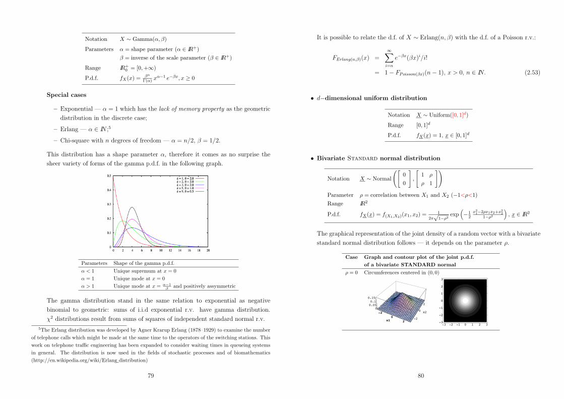
Notation X / Gamma(#,$)
Parameters # = shape parameter (# " IR+)$ = inverse of the scale parameter ($ " IR+)
Range IR+0 = [0,+,)
P.d.f. fX(x) = &"
"(%) x%$1 e$&x, x - 0
Special cases
– Exponential — $ = 1 which has the lack of memory property as the geometric
distribution in the discrete case;
– Erlang — $ " IN ;5
– Chi-square with n degrees of freedom — $ = n/2, ) = 1/2.
This distribution has a shape parameter $, therefore it comes as no surprise the
sheer variety of forms of the gamma p.d.f. in the following graph.
Parameters Shape of the gamma p.d.f.# < 1 Unique supremum at x = 0# = 1 Unique mode at x = 0# > 1 Unique mode at x = !!1
" and positively assymmetric
The gamma distribution stand in the same relation to exponential as negative
binomial to geometric: sums of i.i.d exponential r.v. have gamma distribution.
*2 distributions result from sums of squares of independent standard normal r.v.
5The Erlang distribution was developed by Agner Krarup Erlang (1878–1929) to examine the numberof telephone calls which might be made at the same time to the operators of the switching stations. Thiswork on telephone tra$c engineering has been expanded to consider waiting times in queueing systemsin general. The distribution is now used in the fields of stochastic processes and of biomathematics(http://en.wikipedia.org/wiki/Erlang distribution)
79
It is possible to relate the d.f. of X / Erlang(n, )) with the d.f. of a Poisson r.v.:
FErlang(n,&)(x) =!%
i=n
e$&x()x)i/i!
= 1! FPoisson(&x)(n! 1), x > 0, n " IN. (2.53)
• d!dimensional uniform distribution
Notation X / Uniform([0, 1]d)
Range [0, 1]d
P.d.f. fX(x) = 1, x " [0, 1]d
• Bivariate Standard normal distribution
Notation X / Normal
"B00
C,
B1 &
& 1
C$
Parameter & = correlation between X1 and X2 (!1<&<1)Range IR2
P.d.f. fX(x) = f(X1,X2)(x1, x2) = 1
2!+
1$$2exp
9!1
2x21$2$x1x2+x2
21$$2
:, x " IR2
The graphical representation of the joint density of a random vector with a bivariate
standard normal distribution follows — it depends on the parameter (.
Case Graph and contour plot of the joint p.d.f.of a bivariate STANDARD normal
& = 0 Circumferences centered in (0, 0)
-2
0
2x1-2
0
2
x2
00.05
0.1
0.15
-2
0
2x1
-3 -2 -1 0 1 2 3-3
-2
-1
0
1
2
3
80

Case Graph and contour plot of the joint p.d.f.of a bivariate STANDARD normal (cont.)
& < 0 Ellipses centered in (0, 0) and asymmetric in relation to the axes,suggesting that X2 decreases when X1 increases
-2
0
2x1-2
0
2
x2
00.10.20.3
-2
0
2x1
-3 -2 -1 0 1 2 3-3
-2
-1
0
1
2
3
& > 0 Ellipses centered in (0, 0) and asymmetric in relation to the axes,suggesting that X2 increases when X1 increases
-2
0
2x1-2
0
2
x2
00.10.20.3
-2
0
2x1
-3 -2 -1 0 1 2 3-3
-2
-1
0
1
2
3
Both components of X = (X1, X2) have standard normal marginal densities and X1
and X2 are independent i" ( = 0.
81
2.5 Transformation theory
2.5.1 Transformations of r.v., general case
Motivation 2.70 — Transformations of r.v., general case (Karr, 1993, p. 60)
Let:
• X be a r.v. with d.f. FX ;
• Y = g(X) be a transformation of X under g, where g : IR 4 IR is a Borel measurable
function.
Then we know that Y = g(X) is also a r.v. But this is manifestly not enough: we wish
to know
• how the d.f. of Y relates to that of X?
This question admits an obvious answer when g is invertible and in a few other cases
described below. •
Proposition 2.71 — D.f. of a transformation of a r.v., general case (Rohatgi,
1976, p. 68; Murteira, 1979, p. 121)
Let:
• X be a r.v. with d.f. FX ;
• Y = g(X) be a transformation of X under g, where g : IR 4 IR is a Borel measurable
function;
• g$1((!,, y]) = {x " IR : g(x) ' y} be the inverse image of the Borel set (!,, y]
under g.
Then
FY (y) = P ({Y ' y})= P ({X " g$1((!,, y])}). (2.54)
•
Exercise 2.72 — D.f. of a transformation of a r.v., general case
Prove Proposition 2.71 (Rohatgi, 1976, p. 68).
Note that if g is a Borel measurable function then
g$1(B) " B(IR), (B = (!,, y] " B(IR). (2.55)
82

Thus, we are able to write
P ({Y " B}) = P ({g(X) " B}) = P ({X " g$1(B)}). (2.56)
•
Remark 2.73 — D.f. of a transformation of a r.v., general case
Proposition 2.71 relates the d.f. of Y to that of X.
The inverse image g$1((!,, y]) is a Borel set and tends to be a “reasonable” set —
a real interval or a union of real intervals. •
Exercise 2.74 — D.f. of a transformation of a r.v., general case (Karr, 1993, p.
70, Exercise 2.20(a))
Let X be a r.v. and Y = X2. Prove that
FY (y) = FX(+
y)! FX [!(+
y)$], (2.57)
for y - 0. •
Exercise 2.75 — D.f. of a transformation of a r.v., general case (Rohatgi, 1976,
p. 68)
Let X be a r.v. with d.f. FX . Derive the d.f. of the following r.v.:
(a) |X|
(b) aX + b
(c) eX . •
Exercise 2.76 — D.f. of a transformation of a r.v., absolutely continuous case
The electrical resistance6 (X) of an object and its electrical conductance7 (Y ) are related
as follows: Y = X$1.
Assuming that X / Uniform(900 ohm, 1100 ohm):
(a) Identify the range of values of the r.v. Y .
(b) Derive the survival function of Y , P (Y > y), and calculate P (Y > 10$3 mho). •
6The electrical resistance of an object is a measure of its opposition to thepassage of a steady electric current. The SI unit of electrical resistance is the ohm
(http://en.wikipedia.org/wiki/Electrical resistance).7Electrical conductance is a measure of how easily electricity flows along a certain path through an
electrical element. The SI derived unit of conductance is the siemens (also called the mho, because it isthe reciprocal of electrical resistance, measured in ohms). Oliver Heaviside coined the term in September1885 (http://en.wikipedia.org/wiki/Electrical conductance).
83
Exercise 2.77 — D.f. of a transformation of a r.v., absolutely continuous case
Let X / Uniform(0, 2") and Y = sin X. Prove that
FY (y) =
)*+
*,
0, y < !112 + arcsin y
! , !1 ' y ' 1
1, y > 1.
(2.58)
•
2.5.2 Transformations of discrete r.v.
Proposition 2.78 — P.f. of a one-to-one transformation of a discrete r.v.
(Rohatgi, 1976, p. 69)
Let:
• X be a discrete r.v. with p.f. P ({X = x});
• RX be a countable set such that P ({X " RX}) = 1 and P ({X = x}) > 0,
(x " RX ;
• Y = g(X) be a transformation of X under g, where g : IR 4 IR is a one-to-one
Borel measurable function that transforms RX onto some set RY = g(RX).
Then the inverse map, g$1, is a single-valued function of y and
P ({Y = y}) =
7P ({X = g$1(y)}), y " RY
0, otherwise.(2.59)
•
Exercise 2.79 — P.f. of a one-to-one transformation of a discrete r.v. (Rohatgi,
1976, p. 69)
Let X / Poisson(&). Obtain the p.f. of Y = X2 + 3. •
Exercise 2.80 — P.f. of a one-to-one transformation of a discrete r.v.
Let X / Binomial(n, p) and Y = n!X. Prove that:
• Y / Binomial(n, 1! p);
• FY (y) = 1! FX(n! y ! 1), y = 0, 1, . . . , n. •
Remark 2.81 — P.f. of a transformation of a discrete r.v. (Rohatgi, 1976, p. 69)
Actually the restriction of a single-valued inverse on g is not necessary. If g has a finite (or
even a countable) number of inverses for each y, from the countable additivity property
of probability functions we can obtain the p.f. of the r.v. Y = g(X). •
84

Proposition 2.82 — P.f. of a transformation of a discrete r.v. (Murteira, 1979,
p. 122)
Let:
• X be a discrete r.v. with p.f. P ({X = x});
• RX be a countable set such that P ({X " RX}) = 1 and P ({X = x}) > 0,
(x " RX ;
• Y = g(X) be a transformation of X under g, where g : IR 4 IR is a Borel measurable
function that transforms RX onto some set RY = g(RX);
• Ay = {x " RX : g(x) = y} be a non empty set, for y " RY .
Then
P ({Y = y}) = P ({X " Ay})=
%
x"Ay
P ({X = x}), (2.60)
for y " RY . •
Exercise 2.83 — P.f. of a transformation of a discrete r.v. (Rohatgi, 1976, pp.
69–70)
Let X be a discrete r.v. with p.f.
P ({X = x}) =
)********+
********,
15 , x = !216 , x = !115 , x = 0115 , x = 11130 , x = 2
0, otherwise
(2.61)
Derive the p.f. of Y = X2. •
85
2.5.3 Transformations of absolutely continuous r.v.
Proposition 2.84 — D.f. of a strictly monotonic transformation of an
absolutely continuous r.v. (Karr, 1993, pp. 60 and 68)
Let:
• X be an absolutely continuous r.v. with d.f. FX and p.d.f. fX ;
• RX be the range of the r.v. X, i.e. RX = {x " IR : fX(x) > 0};
• Y = g(X) be a transformation of X under g, where g : IR 4 IR is a continuous,
strictly increasing, Borel measurable function that transforms RX onto some set
RY = g(RX);
• g$1 be the pointwise inverse of g.
Then
FY (y) = FX [g$1(y)], (2.62)
for y " RY . Similarly, if
• g is a continuous, strictly decreasing, Borel measurable function
then
FY (y) = 1! FX [g$1(y)], (2.63)
for y " RY . •
Exercise 2.85 — D.f. of a strictly monotonic transformation of an absolutely
continuous r.v.
Prove Proposition 2.84 (Karr, 1993, p. 60). •
Exercise 2.86 — D.f. of a strictly monotonic transformation of an absolutely
continuous r.v.
Let X / Normal(0, 1). Derive the d.f. of
(a) Y = eX
(b) Y = µ + #X, where µ " IR and # " IR+
(Karr, 1993, p. 60). •
86

Remark 2.87 — Transformations of absolutely continuous and discrete r.v.
(Karr, 1993, p. 61)
in general, Y = g(X) need not be absolutely continuous even when X is, as shown in the
next exercise, while if X is a discrete r.v. then so is Y = g(X) regardless of the Borel
measurable function g. •
Exercise 2.88 — A mixed r.v. as a transformation of an absolutely continuous
r.v.
Let X / Uniform(!1, 1). Prove that Y = X+ = max{0, X} is a mixed r.v. whose d.f. is
given by
FY (y) =
)***+
***,
0, y < 012 , y = 012 + y
2 , 0 < y ' 1
1, y > 1
(2.64)
(Rohatgi, 1976, p. 70). •
Exercise 2.88 shows that we need some conditions on g to ensure that Y = g(X) is
also an absolutely continuous r.v. This will be the case when g is a continuous monotonic
function.
Theorem 2.89 — P.d.f. of a strictly monotonic transformation of an absolutely
continuous r.v. (Rohatgi, 1976, p. 70; Karr, 1993, p. 61)
Suppose that:
• X is an absolutely continuous r.v. with p.d.f. fX ;
• there is an open subset RX # IR such that P ({X " RX}) = 1;
• Y = g(X) is a transformation of X under g, where g : IR 4 IR is a continuously
di"erentiable, Borel measurable function such that either dg(x)dx > 0, (x " RX , or
dg(x)dx < 0, (x " RX ;8
• g transforms RX onto some set RY = g(RX);
• g$1 represents the pointwise inverse of g.
8This implies that dg(x)dx &= 0, (x " RX .
87
Then Y = g(X) is an absolutely continuous r.v. with p.d.f. given by
fY (y) = fX [g$1(y)])DDDDdg$1(y)
dy
DDDD , (2.65)
for y " RY . •
Exercise 2.90 — P.d.f. of a strictly monotonic transformation of an absolutely
continuous r.v.
Prove Theorem 2.89 by considering the case dg(x)dx > 0, (x " RX , applying Proposition 2.84
to derive the d.f. of Y = g(X), and di"erentiating it to obtain the p.d.f. of Y (Rohatgi,
1976, p. 70). •
Remark 2.91 — P.d.f. of a strictly monotonic transformation of an absolutely
continuous r.v. (Rohatgi, 1976, p. 71)
The key to computation of the induced d.f. of Y = g(X) from the d.f. of X is P ({Y 'y}) = P ({X " g$1((!,, y])}). If the conditions of Theorem 2.89 are satisfied, we are
able to identify the set {X " g$1((!,, y])} as {X ' g$1(y)} or {X - g$1(y)}, according
to whether g in strictly increasing or strictly decreasing. •
Exercise 2.92 — P.d.f. of a strictly monotonic transformation of an absolutely
continuous r.v.
Let X / Normal(0, 1). Identify the p.d.f. and the distribution of
(a) Y = eX
(b) Y = µ + #X, where µ " IR and # " IR+
(Karr, 1993, p. 61). •
Corollary 2.93 — P.d.f. of a strictly monotonic transformation of an absolutely
continuous r.v. (Rohatgi, 1976, p. 71)
Under the conditions of Theorem 2.89, and by noting that
dg$1(y)
dy=
1dg(x)
dx
DDDDDx=g!1(y)
, (2.66)
we conclude that the p.d.f. of Y = g(X) can be rewritten as follows:
fY (y) =fX(x)DDDdg(x)
dx
DDD
DDDDDDx=g!1(y)
, (2.67)
(y " RY . •
88

Remark 2.94 — P.d.f. of a non monotonic transformation of an absolutely
continuous r.v. (Rohatgi, 1976, p. 71)
In practice Theorem 2.89 is quite useful, but whenever its conditions are violated we
should return to P ({Y ' y}) = P ({X " g$1((!,, y])}) to obtain the FY (y) and then
di"erentiate this d.f. to derive the p.d.f. of the transformation Y . This is the case in the
next two exercises. •
Exercise 2.95 — P.d.f. of a non monotonic transformation of an absolutely
continuous r.v.
Let X / Normal(0, 1) and Y = g(X) = X2. Prove that Y / *2(1) by noting that
FY (y) = FX(+
y)! FX(!+y), y > 0 (2.68)
fY (y) =dFY (y)
dy
=
71
2%
y )/fX(
+y) + fX(!+y)
0, y - 0
0, y < 0(2.69)
(Rohatgi, 1976, p. 72). •
Exercise 2.96 — P.d.f. of a non monotonic transformation of an absolutely
continuous r.v.
Let X be an absolutely continuous r.v. with p.d.f.
fX(x) =
72x!2 , 0 < x < "
0, otherwise(2.70)
Prove that Y = sin X has p.d.f. given by
fY (y) =
72
!+
1$y2, 0 < y < 1
0, otherwise(2.71)
(Rohatgi, 1976, p. 73). •
Motivation 2.97 — P.d.f. of a sum of monotonic restrictions of a function g of
an absolutely continuous r.v. (Rohatgi, 1976, pp. 73–74)
in the two last exercises the function y = g(x) can be written as the sum of two monotonic
restrictions of g in two disjoint intervals. Therefore we can apply Theorem 2.89 to each
of these monotonic summands.
In fact, these two exercises are special cases of the following theorem. •
89
Theorem 2.98 — P.d.f. of a finite sum of monotonic restrictions of a function
g of an absolutely continuous r.v. (Rohatgi, 1976, pp. 73–74)
Let:
• X be an absolutely continuous r.v. with p.d.f. fX ;
• Y = g(X) be a transformation of X under g, where g : IR 4 IR is a Borel measurable
function that transforms RX onto some set RY = g(RX).
Moreover, suppose that:
• g(x) is di"erentiable for all x " RX ;
• dg(x)dx is continuous and nonzero at all points of RX but a finite number of x.
Then, for every real number y " RY ,
(a) there is a positive integer n = n(y) and real numbers (inverses) g$11 (y), . . . , g$1
n (y)
such that
g(x)|x=g!1k (y) = y and
dg(x)
dx
DDDDx=g!1
k (y)
&= 0, k = 1, . . . , n(y), (2.72)
or
(b) there is not an x such that g(x) = y and dg(x)dx &= 0, in which case we write n =
n(y) = 0.
In addition, Y = g(X) is an absolutely continuous r.v. with p.d.f. given by
fY (y) =
7 !n(y)k=1 fX [g$1
k (y)])DDDdg!1
k (y)
dy
DDD , n = n(y) > 0
0, n = n(y) = 0,(2.73)
for y " RY . •
Exercise 2.99 — P.d.f. of a finite sum of monotonic restrictions of a function
g of an absolutely continuous r.v.
Let X / Uniform(!1, 1). Use Theorem 2.98 to prove that Y = |X| / Uniform(0, 1)
(Rohatgi, 1976, p. 74). •
Exercise 2.100 — P.d.f. of a finite sum of monotonic restrictions of a function
g of an absolutely continuous r.v.
Let X / Uniform(0, 2") and Y = sin X. Use Theorem 2.98 to prove that
fY (y) =
71
!+
1$y2, !1 < y < 1
0, otherwise.(2.74)
•
90

Motivation 2.101 — P.d.f. of a countable sum of monotonic restrictions of a
function g of an absolutely continuous r.v.
The formula P ({Y ' y}) = P ({X " g$1((!,, y])}) and the countable additivity of
probability functions allows us to compute the p.d.f. of Y = g(X) in some instance even
if g has a countable number of inverses. •
Theorem 2.102 — P.d.f. of a countable sum of monotonic restrictions of a
function g of an absolutely continuous r.v. (Rohatgi, 1976, pp. 74–75)
Let g be a Borel measurable function that maps RX onto some set RY = g(RX). Suppose
that RX can be represented as a countable union of disjoint sets Ak, k = 1, 2, . . . Then
Y = g(X) is an absolutely continuous r.v. with d.f. given by
FY (y) = P ({Y ' y})= P ({X " g$1((!,, y])})
= P
"7X "
+!#
k=1
/g$1((!,, y]) $ Ak
0=$
=+!%
k=1
P-E
X "/g$1((!,, y]) $ Ak
0F., y " RY . (2.75)
If the conditions of Theorem 2.89 are satisfied by the restriction of g to each Ak, gk,
we may obtain the p.d.f. of Y = g(X) on di"erentiating the d.f. of Y .9 In this case
fY (y) =+!%
k=1
fX [g$1k (y)])
DDDDdg$1
k (y)
dy
DDDD , y " RY . (2.76)
•
Exercise 2.103 — P.d.f. of a countable sum of monotonic restrictions of a
function g of an absolutely continuous r.v.
Let X / Exponential(&) and Y = sin X. Prove that
FY (y) = 1 +e$"!+" arcsin y ! e$" arcsin y
1! e$2!", 0 < y < 1 (2.77)
fY (y) =
)**+
**,
"e!#$
(1$e!2#$)/+
1$y2)
-e" arcsin y + e$"!$" arcsin y
., !1 ' y < 0
"
(1$e!2#$)/+
1$y2)
-e$" arcsin y + e$"!+" arcsin y
., 0 ' y < 1
0, otherwise
(2.78)
(Rohatgi, 1976, p. 75). •
9We remind the reader that term-by-term di"erentiation is permissible if the di"erentiated series isuniformly convergent.
91
2.5.4 Transformations of random vectors, general case
What follows is the analogue of Proposition 2.71 in a multidimensional setting.
Proposition 2.104 — D.f. of a transformation of a random vector, general case
Let:
• X = (X1, . . . , Xd) be a random vector with joint d.f. FX ;
• Y = (Y1, . . . , Ym) = g(X) = (g1(X1, . . . , Xd), . . . , gm(X1, . . . , Xd)) be a
transformation of X under g, where g : IRd 4 IRm is a Borel measurable function;
• g$1(Am
i=1(!,, yi]) = {x = (x1, . . . , xd) " IRd : g1(x1, . . . , xd) ' y1, . . .,
gm(x1, . . . , xd) ' ym} be the inverse image of the Borel setAm
i=1(!,, yi] under
g.10
Then
FY (y) = P ({Y1 ' y1, . . . , Ym ' ym})
= P
"7X " g$1
"m&
i=1
(!,, yi]
$=$. (2.79)
•
Exercise 2.105 — D.f. of a transformation of a random vector, general case
Let X = (X1, . . . , Xd) be an absolutely continuous random vector such that
Xiindep/ Exponential(&i), i = 1, . . . , d.
Prove that Y = mini=1,...,d Xi / Exponential(!d
i=1 &i). •
2.5.5 Transformations of discrete random vectors
Theorem 2.106 — Joint p.f. of a one-to-one transformation of a discrete
random vector (Rohatgi, 1976, p. 131)
Let:
• X = (X1, . . . , Xd) be a discrete random vector with joint p.f. P ({X = x});
• RX be a countable set of points such that P (X " RX) = 1 and P ({X = x) > 0,
(x " IRX ;
10Let us remind the reader that since g is a Borel measurable function we have g!1(B) " B(IRd), (B "B(IRm).
92
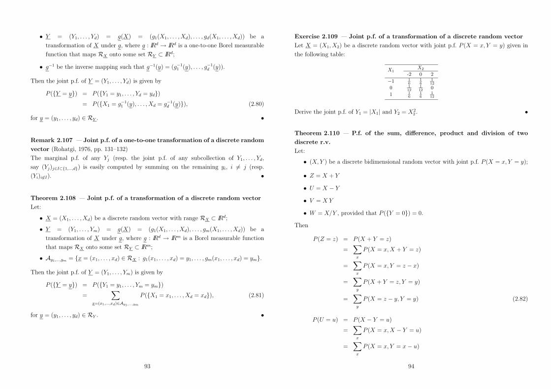
• Y = (Y1, . . . , Yd) = g(X) = (g1(X1, . . . , Xd), . . . , gd(X1, . . . , Xd)) be a
transformation of X under g, where g : IRd 4 IRd is a one-to-one Borel measurable
function that maps RX onto some set RY # IRd;
• g$1 be the inverse mapping such that g$1(y) = (g$11 (y), . . . , g$1
d (y)).
Then the joint p.f. of Y = (Y1, . . . , Yd) is given by
P ({Y = y}) = P ({Y1 = y1, . . . , Yd = yd})= P ({X1 = g$1
1 (y), . . . , Xd = g$1d (y)}), (2.80)
for y = (y1, . . . , yd) " RY . •
Remark 2.107 — Joint p.f. of a one-to-one transformation of a discrete random
vector (Rohatgi, 1976, pp. 131–132)
The marginal p.f. of any Yj (resp. the joint p.f. of any subcollection of Y1, . . . , Yd,
say (Yj)j"I0{1,...,d}) is easily computed by summing on the remaining yi, i &= j (resp.
(Yi)i."I). •
Theorem 2.108 — Joint p.f. of a transformation of a discrete random vector
Let:
• X = (X1, . . . , Xd) be a discrete random vector with range RX # IRd;
• Y = (Y1, . . . , Ym) = g(X) = (g1(X1, . . . , Xd), . . . , gm(X1, . . . , Xd)) be a
transformation of X under g, where g : IRd 4 IRm is a Borel measurable function
that maps RX onto some set RY # IRm;
• Ay1,...,ym = {x = (x1, . . . , xd) " RX : g1(x1, . . . , xd) = y1, . . . , gm(x1, . . . , xd) = ym}.
Then the joint p.f. of Y = (Y1, . . . , Ym) is given by
P ({Y = y}) = P ({Y1 = y1, . . . , Ym = ym})=
%
x=(x1,...,xd)"Ay1,...,ym
P ({X1 = x1, . . . , Xd = xd}), (2.81)
for y = (y1, . . . , yd) " RY . •
93
Exercise 2.109 — Joint p.f. of a transformation of a discrete random vector
Let X = (X1, X2) be a discrete random vector with joint p.f. P (X = x, Y = y) given in
the following table:
X2X1-2 0 2
!1 16
16
112
0 112
112 0
1 16
16
112
Derive the joint p.f. of Y1 = |X1| and Y2 = X22 . •
Theorem 2.110 — P.f. of the sum, di!erence, product and division of two
discrete r.v.
Let:
• (X, Y ) be a discrete bidimensional random vector with joint p.f. P (X = x, Y = y);
• Z = X + Y
• U = X ! Y
• V = X Y
• W = X/Y , provided that P ({Y = 0}) = 0.
Then
P (Z = z) = P (X + Y = z)
=%
x
P (X = x, X + Y = z)
=%
x
P (X = x, Y = z ! x)
=%
y
P (X + Y = z, Y = y)
=%
y
P (X = z ! y, Y = y) (2.82)
P (U = u) = P (X ! Y = u)
=%
x
P (X = x, X ! Y = u)
=%
x
P (X = x, Y = x! u)
94

=%
y
P (X ! Y = u, Y = y)
=%
y
P (X = u + y, Y = y) (2.83)
P (V = v) = P (X Y = v)
=%
x
P (X = x, XY = v)
=%
x
P (X = x, Y = v/x)
=%
y
P (XY = v, Y = y)
=%
y
P (X = v/y, Y = y) (2.84)
P (W = w) = P (X/Y = w)
=%
x
P (X = x, X/Y = w)
=%
x
P (X = x, Y = x/w)
=%
y
P (X/Y = w, Y = y)
=%
y
P (X = wy, Y = y). (2.85)
•
Exercise 2.111 — P.f. of the di!erence of two discrete r.v.
Let (X, Y ) be a discrete random vector with joint p.f. P (X = x, Y = y) given in the
following table:
YX1 2 3
1 112
112
212
2 212 0 0
3 112
112
412
(a) Prove that X and Y are identically distributed but are not independent.
(b) Obtain the p.f. of U = X ! Y
(c) Prove that U = X!Y is not a symmetric r.v., that is U and !U are not identically
distributed. •
95
Corollary 2.112 — P.f. of the sum, di!erence, product and division of two
independent discrete r.v.
Let:
• X and Y be two independent discrete r.v. with joint p.f. P (X = x, Y = y) =
P (X = x)) P (Y = y), (x, y
• Z = X + Y
• U = X ! Y
• V = X Y
• W = X/Y , provided that P ({Y = 0}) = 0.
Then
P (Z = z) = P (X + Y = z)
=%
x
P (X = x)) P (Y = z ! x)
=%
y
P (X = z ! y)) P (Y = y) (2.86)
P (U = u) = P (X ! Y = u)
=%
x
P (X = x)) P (Y = x! u)
=%
y
P (X = u + y)) P (Y = y) (2.87)
P (V = v) = P (X Y = v)
=%
x
P (X = x)) P (Y = v/x)
=%
y
P (X = v/y)) P (Y = y) (2.88)
P (W = w) = P (X/Y = w)
=%
x
P (X = x)) P (Y = x/w)
=%
y
P (X = wy)) P (Y = y). (2.89)
•
96
Exercise 2.113 — P.f. of the sum of two independent r.v. with three well
known discrete distributions
Let X and Y be two independent discrete r.v. Prove that
(a) X / Binomial(nX , p) :: Y / Binomial(nY , p) . (X + Y ) / Binomial(nX + nY , p)
(b) X / NegativeBinomial(nX , p) :: Y / NegativeBinomial(nY , p) . (X + Y ) /NegativeBinomial(nX + nY , p)
(c) X / Poisson(&X) :: Y / Poisson(&Y ) . (X + Y ) / Poisson(&X + &Y ),
i.e. the families of Poisson, Binomial and Negative Binomial distributions are closed under
summation of independent members.11 •
Exercise 2.114 — P.f. of the di!erence of two independent Poisson r.v.
Let X / Poisson(&X) :: Y / Poisson(&Y ). Then (X ! Y ) has p.f. given by
P (X ! Y = u) =+!%
y=0
P (X = u + y)) P (Y = y)
= e$("X+"Y )+!%
y=max{0,$u}
&u+yX &y
Y
(u + y)! y!, u = . . . ,!1, 0, 1, . . . (2.90)
•
Remark 2.115 — Skellam distribution (http://en.wikipedia.org/wiki/
Skellam distribution)
The Skellam distribution is the discrete probability distribution of the di"erence of
independent r.v. X and Y having Poisson distributions with parameters &X and &Y .
It is useful in describing the statistics of the di"erence of two images with simple photon
noise, as well as describing the point spread distribution in certain sports where all scored
points are equal, such as baseball, hockey and soccer.
When &X = &Y = & and u is also large, and of order of the square root of 2&,
P (X ! Y = u) * e$u2
2"2#
+2" ) 2&
, (2.91)
the p.d.f. of a Normal distribution with parameters µ = 0 and #2 = 2&.
Please note that the expression of the p.f. of the Skellam distribution that can be
found in http://en.wikipedia.org/wiki/Skellam distribution is not correct. •
11Use the Vandermonde’s identity to prove result (a). In combinatorial mathematics,Vandermonde’s identity, named after Alexandre-Theophile Vandermonde (1772), states that theequality
-m+nr
.=
!rk=0
-mk
.- nr!k
., m, n, r " IN0, for binomial coe$cients holds; this
identity was given already in 1303 by the Chinese mathematician Zhu Shijie (Chu Shi-Chieh)(http://en.wikipedia.org/wiki/Vandermonde’s identity).
97
2.5.6 Transformations of absolutely continuous random vectors
Motivation 2.116 — P.d.f. of a transformation of an absolutely continuous
random vector (Karr, 1993, p. 62)
Recall that a random vector X = (X1, . . . , Xd) is absolutely continuous if there is a
function fX on IRd satisfying
FX(x) = FX1,...,Xd(x1, . . . , xd)
=
6 x1
$!. . .
6 xd
$!fX1,...,Xd
(s1, . . . , sd) dsd . . . ds1. (2.92)
Computing the density of Y = g(X) requires that g be invertible, except for the special
case that X1, . . . , Xd are independent (and then only for particular choices of g). •
Theorem 2.117 — P.d.f. of a one-to-one transformation of an absolutely
continuous random vector (Rohatgi, 1976, p. 135; Karr, 1993, p. 62)
Let:
• X = (X1, . . . , Xd) be an absolutely continuous random vector with joint p.d.f. fX(x);
• RX be an open set of IRd such that P (X " RX) = 1;
• Y = (Y1, . . . , Yd) = g(X) = (g1(X1, . . . , Xd), . . . , gd(X1, . . . , Xd)) be a
transformation of X under g, where g : IRd 4 IRd is a one-to-one Borel measurable
function that maps RX onto some set RY # IRd;
• g$1(y) = (g$11 (y), . . . , g$1
d (y)) be the inverse mapping defined over the range RY of
the transformation.
Assume that:
• both g and its inverse g$1 are continuous;
• the partial derivatives,'g!1
i (y)
'yj, 1 ' i, j ' d, exist and are continuous;
• the Jacobian of the inverse transformation g$1 (i.e. the determinant of the matrix
of partial derivatives'g!1
i (y)
'yj) is such that
J(y) =
DDDDDDDD
'g!11 (y)
'y1· · · 'g!1
1 (y)
'yd... · · · ...
'g!1d (y)
'y1· · · 'g!1
d (y)
'yd
DDDDDDDD&= 0, (2.93)
for y = (y1, . . . , yd) " RY .
98

Then the random vector Y = (Y1, . . . , Yd) is absolutely continuous and its joint p.d.f. is
given by
fY (y) = fX
/g$1(y)
0) |J(y)|, (2.94)
for y = (y1, . . . , yd) " RY . •
Exercise 2.118 — P.d.f. of a one-to-one transformation of an absolutely
continuous random vector
Prove Theorem 2.117 (Rohatgi, 1976, pp. 135–136). •
Exercise 2.119 — P.d.f. of a one-to-one transformation of an absolutely
continuous random vector
Let
• X = (X1, . . . , Xd) be an absolutely continuous random vector with joint p.d.f. fX(x);
• Y = (Y1, . . . , Yd) = g(X) = AX +b be an invertible a$ne mapping of IRd into itself,
where A is a nonsingular d) d matrix and b " IRd.
Derive the inverse mapping g$1 and the joint p.d.f. of Y (Karr, 1993, p. 62). •
Exercise 2.120 — P.d.f. of a one-to-one transformation of an absolutely
continuous random vector
Let
• X = (X1, X2, X3) such that Xii.i.d./ Exponential(1);
• Y = (Y1, Y2, Y3) =9X1 + X2 + X3,
X1+X2X1+X2+X3
, X1X1+X2
:.
Derive the joint p.d.f. of Y and conclude that Y1, Y2, and Y3 are also independent (Rohatgi,
1976, p. 137). •
Remark 2.121 — P.d.f. of a one-to-one transformation of an absolutely
continuous random vector (Rohatgi, 1976, p. 136)
In actual applications, we tend to know just k functions, Y1 = g1(X), . . . , Yk = gk(X).
In this case, we introduce arbitrarily (d! k) (convenient) r.v., Yk+1 = gk+1(X), . . . , Yd =
gd(X)), such that the conditions of Theorem 2.117 are satisfied.
To find the joint density of the k r.v. we simply integrate the joint p.d.f. fY over all
the (d! k) r.v. that were arbitrarily introduced. •
We can state a similar result to Theorem 2.117 when g is not a one-to-one
transformation.
99
Theorem 2.122 — P.d.f. of a transformation, with a finite number of inverses,
of an absolutely continuous random vector (Rohatgi, 1976, pp. 136–137)
Assume the conditions of Theorem 2.117 and suppose that:
• for each y " RY # IRd, the transformation g has a finite number k = k(y) of
inverses;
• RX # IRd can be partitioned into k disjoint sets, A1, . . . , Ak, such that the
transformation g from Ai (i = 1, . . . , k) into IRd, say gi, is one-to-one with inverse
transformation g$1i
= (g$11 i (y), . . . , g$1
d i (y)), i = 1, . . . , k;
• the first partial derivatives of g$1i
exist, are continuous and that each Jacobian
Ji(y) =
DDDDDDDD
'g!11 i (y)
'y1· · · 'g!1
1 i (y)
'yd... · · · ...
'g!1d i (y)
'y1· · · 'g!1
d i (y)
'yd
DDDDDDDD&= 0, (2.95)
for y = (y1, . . . , yd) in the range of the transformation gi.
Then the random vector Y = (Y1, . . . , Yd) is absolutely continuous and its joint p.d.f. is
given by
fY (y) =k%
i=1
fX
Gg$1
i(y)
H) |Ji(y)|, (2.96)
for y = (y1, . . . , yd) " RY . •
Theorem 2.123 — P.d.f. of the sum, di!erence, product and division of two
absolutely continuous r.v. (Rohatgi, 1976, p. 141)
Let:
• (X, Y ) be an absolutely continuous bidimensional random vector with joint p.d.f.
fX,Y (x, y);
• Z = X + Y , U = X ! Y , V = X Y and W = X/Y .
Then
fZ(z) = fX+Y (z)
=
6 +!
$!fX,Y (x, z ! x) dx
=
6 +!
$!fX,Y (z ! y, y) dy (2.97)
100

fU(u) = fX$Y (u)
=
6 +!
$!fX,Y (x, x! u) dx
=
6 +!
$!fX,Y (u + y, y) dy (2.98)
fV (v) = fXY (v)
=
6 +!
$!fX,Y (x, v/x)) 1
|x| dx
=
6 +!
$!fX,Y (v/y, y)) 1
|y| dy (2.99)
fW (w) = fX/Y (w)
=
6 +!
$!fX,Y (x, x/w)) |x|
w2dx
=
6 +!
$!fX,Y (wy, y)) |y| dy. (2.100)
•
Remark 2.124 — P.d.f. of the sum and product of two absolutely continuous
r.v.
It is interesting to note that:
fZ(z) =d FZ(z)
dz
=d P (Z = X + Y ' z)
dz
=d
dz
I6 6
{(x,y): x+y'z}fX,Y (x, y) dy dx
J
=d
dz
I6 +!
$!
6 z$x
$!fX,Y (x, y) dy dx
J
=
6 +!
$!
d
dz
I6 z$x
$!fX,Y (x, y) dy
Jdx
=
6 +!
$!fX,Y (x, z ! x) dx; (2.101)
fV (v) =d FV (v)
dv
=d P (V = XY ' v)
dv
101
=d
dv
I6 6
{(x,y): xy'v}fX,Y (x, y) dy dx
J
=
)+
,
@ +!$!
ddv
G@ v/x
$! fX,Y (x, y) dyH
dx, x > 0@ +!$!
ddv
G@ +!v/x fX,Y (x, y) dy
Hdx, x < 0
=
6 +!
$!
1
|x| fX,Y (x, v/x) dx. (2.102)
•
Corollary 2.125 — P.d.f. of the sum, di!erence, product and division of two
independent absolutely continuous r.v. (Rohatgi, 1976, p. 141)
Let:
• X and Y be two independent absolutely continuous r.v. with joint p.d.f.
fX,Y (x, y) = fX(x)) fY (y), (x, y;
• Z = X + Y , U = X ! Y , V = X Y and W = X/Y .
Then
fZ(z) = fX+Y (z)
=
6 +!
$!fX(x)) fY (z ! x) dx
=
6 +!
$!fX(z ! y)) fY (y) dy (2.103)
fU(u) = fX$Y (u)
=
6 +!
$!fX(x)) fY (x! u) dx
=
6 +!
$!fX(u + y)fY (y) dy (2.104)
fV (v) = fXY (v)
=
6 +!
$!fX(x)) fY (v/x)) 1
|x| dx
=
6 +!
$!fX(v/y)) fY (y)) 1
|y| dy (2.105)
fW (w) = fX/Y (w)
=
6 +!
$!fX(x)) fY (x/w)) |x|
w2dx
102

=
6 +!
$!fX(wy)) fY (y)) |y| dy. (2.106)
•
Exercise 2.126 — P.d.f. of the sum and di!erence of two independent
absolutely continuous r.v.
Let X and Y be two r.v. which are independent and uniformly distributed in (0, 1). Derive
the p.d.f. of:
(a) (X + Y, X ! Y ) (Rohatgi, 1976, pp. 137–138);
(b) X + Y ;
(c) X ! Y . •
Exercise 2.127 — P.d.f. of the mean of two independent absolutely continuous
r.v.
Let X and Y be two independent r.v. with standard normal distribution. Prove that their
mean X+Y2 / Normal(0, 2$1). •
Remark 2.128 — D.f. and p.d.f. of the sum, di!erence, product and division
of two absolutely continuous r.v.
In several cases it is simpler to obtain the d.f. of those four algebraic functions of X and
Y than to derive the corresponding p.d.f. It su$ces to apply Proposition 2.104 and then
di"erentiate the d.f. to get the p.d.f., as seen in the next exercises. •
Exercise 2.129 — D.f. and p.d.f. of the di!erence of two absolutely continuous
r.v.
Choosing adequate underkeel clearance (UKC) is one of the most crucial and most di$cult
problems in the navigation of large ships, especially very large crude oil carriers.
Let X be the water depth in a passing shallow waterway, say a harbour or a channel,
and Y be the maximum ship draft. Then the probability of a safe passing a shallow
waterway can be expressed as P (UKC = X ! Y > 0).
Assume that X and Y are independent r.v. such that X / Gamma(n, )) and Y /Gamma(m, )), where n, m " IN and m < n. Derive an expression for P (UKC = X!Y >
0) taking into account that FGamma(k,&)(x) =!!
i=k e$&x()x)i/i!, k " IN . •
103
Exercise 2.130 — D.f. and p.d.f. of the sum of two absolutely continuous r.v.
Let X and Y be the durations of two independent system components set in what is called
a stand by connection.12 In this case the system duration is given by X + Y .
Prove that the p.d.f. of X + Y equals
fX+Y (z) =$)
-e$&z ! e$%z
.
$! ), z > 0,
if X / Exponencial($) and Y / Exponencial()), where $, ) > 0 and $ &= ). •
Exercise 2.131 — D.f. of the division of two absolutely continuous r.v.
Let X and Y be the intensity of a transmitted signal and its damping until its reception,
respectively. Moreover, W = X/Y represents the intensity of the received signal.
Assume that the joint p.d.f. of (X, Y ) equals fX,Y (x, y) = &µe$("x+µy) )I(0,+!)/(0,+!)(x, y). Prove that the d.f. of W = X/Y is given by:
FW (w) =
'1! µ
µ + &w
() I(0,+!)(w). (2.107)
•
12At time 0, only the component with duration X is on. The component with duration Y replaces theother one as soon as it fails.
104
2.5.7 Random variables with prescribed distributions
Motivation 2.132 — Construction of a r.v. with a prescribed distribution (Karr,
1993, p. 63)
Can we construct (or simulate) explicitly individual r.v., random vectors or sequences of
r.v. with prescribed distributions? •
Proposition 2.133 — Construction of a r.v. with a prescribed d.f. (Karr, 1993,
p. 63)
Let F be a d.f. on IR. Then there is a probability space (!,F , P ) and a r.v. X defined
on it such that FX = F . •
Exercise 2.134 — Construction of a r.v. with a prescribed d.f.
Prove Proposition 2.133 (Karr, 1993, p. 63). •
The construction of a r.v. with a prescribed d.f. depends on the following definition.
Definition 2.135 — Quantile function (Karr, 1993, p. 63)
The inverse function of F , F$1, or quantile function associated with F , is defined by
F$1(p) = inf{x : F (x) - p}, p " (0, 1). (2.108)
This function is often referred to as the generalized inverse of the d.f. •
Exercise 2.136 — Quantile functions of an absolutely continuous and a discrete
r.v.
Obtain and draw the graphs of the d.f. and quantile function of:
(a) X / Exponential(&);
(b) X / Bernoulli(+).
•
105
Remark 2.137 — Existence of a quantile function (Karr, 1993, p. 63)
Even though F need be neither continuous nor strictly increasing, F$1 always exists.
As the figure of the quantile function (associated with the d.f.) of X / Bernoulli(+),
F$1 jumps where F is flat, and is flat where F jumps.
Although not necessarily a pointwise inverse of F , F$1 serves that role for many
purposes and has a few interesting properties. •
Proposition 2.138 — Basic properties of the quantile function (Karr, 1993, p.
63)
Let F$1 be the (generalized) inverse of F or quantile function associated with F . Then
1. For each p and x,
F$1(p) ' x i" p ' F (x); (2.109)
2. F$1 is non decreasing and left-continuous;
3. If F is absolutely continuous, then
F [F$1(p)] = p, (p " (0, 1). (2.110)
•
Motivation 2.139 — Quantile transformation (Karr, 1993, p. 63)
A r.v. with d.f. F can be constructed by applying F$1 to a r.v. with distribution on (0, 1).
This is usually known as quantile transformation and is a very popular transformation in
random numbers generation/simulation on computer. •
Proposition 2.140 — Quantile transformation (Karr, 1993, p. 64)
Let F be a d.f. on IR and suppose U / Uniform(0, 1). Then
X = F$1(U) has distribution function F. (2.111)
•
Exercise 2.141 — Quantile transformation
Prove Proposition 2.140 (Karr, 1993, p. 64). •
Example 2.142 — Quantile transformation
If U / Uniform(0, 1) then both ! 1" ln(1!U) and ! 1
" ln(U) have exponential distribution
with parameter & (& > 0). •
106

Remark 2.143 — Quantile transformation (Karr, 1993, p. 64)
R.v. with d.f. F can be simulated by applying F$1 to the (uniformly distributed) values
produced by the random number generator.
Feasibility of this technique depends on either having F$1 available in closed form or
being able to approximate it numerically. •
Proposition 2.144 — The quantile transformation and the simulation of
discrete and absolutely continuous distributions
To generate (pseudo-)random numbers from a r.v. X with d.f. F , it su$ces to:
1. Generate a (pseudo-)random number u from the Uniform(0, 1) distribution.
2. Assign
x = F$1(u) = inf{m " IR : F (m) - u}, (2.112)
the quantile of order u of X, where F$1 represents the generalized inverse of F . •
For a detailed discussion on (pseudo-)random number generation/generators and their
properties please refer to Gentle (1998, pp. 6–22). For a brief discussion — in Portuguese
— on (pseudo-)random number generation and Monte Carlo simulation method we refer
the reader to Morais (2003, Chapter 2).
Exercise 2.145 — The quantile transformation and the generation of the
Logistic distribution
X is said to have a Logistic(µ, #) if its p.d.f. is given by
f(x) =e$
x!µ!
#91 + e$
x!µ!
:2 ,!, < x < +,. (2.113)
Define the quantile transformation to produce (pseudo-)random numbers with such a
distribution. •
Exercise 2.146 — The quantile transformation and the simulation of the
Erlang distribution
Describe a method to generate (pseudo-)random numbers from the Erlang(n, &).13 •
13Let us remind the reader that the sum of n independent exponential distributions with parameter "
has an Erlang(n, ").
107
Exercise 2.147 — The quantile transformation and the generation of the Beta
distribution
Let Y and Z be two independent r.v. with distributions Gamma($, &) and Gamma(), &),
respectively ($, ), & > 0).
(a) Prove that X = Y/(Y + Z) / Beta($, )).
(b) Use this result to describe a random number generation method for the Beta($, )),
where $, ) " IN .
(c) Use any software you are familiar with to generate and plot the histogram of 1000
observations from the Beta(4, 5) distribution. •
Example 2.148 — The quantile transformation and the generation of the
Bernoulli distribution (Gentle, 1993, p. 47)
To generate (pseudo-)random numbers from the Bernoulli(p) distribution, we should
proceed as follows:
1. Generate a (pseudo-)random number u from the Uniform(0, 1) distribution.
2. Assign
x =
70, if u ' 1! p
1, if u > 1! p(2.114)
or, equivalently,
x =
70, if u - p
1, if u < p.(2.115)
(Is there any advantage of (2.115) over (2.114)?) •
Exercise 2.149 — The quantile transformation and the simulation of the
Binomial distribution
Describe a method to generate (pseudo-)random numbers from a Binomial(n, p)
distribution. •
Proposition 2.150 — The converse of the quantile transformation (Karr, 1993,
p. 64)
A converse of the quantile transformation (Propositon 2.140) holds as well, under certain
conditions. In fact, if FX is continuous (not necessarily absolutely continuous) then
FX(X) / Uniform(0, 1). (2.116)
•
108
Exercise 2.151 — The converse of the quantile transformation
Prove Propositon 2.150 (Karr, 1993, p. 64). •
Motivation 2.152 — Construction of random vectors with a prescribed
distribution (Karr, 1993, p. 65)
The construction of a random vector with an arbitrary d.f. is more complicated. We shall
address this issue in the next chapter for a special case: when the random vector has
independent components. However, we can state the following result. •
Proposition 2.153 — Construction of a random vector with a prescribed d.f.
(Karr, 1993, p. 65)
Let F : IRd 4 [0, 1] be a d!dimensional d.f. Then there is a probability space (!,F , P )
and a random vector X = (X1, . . . , Xd) defined on it such that FX = F . •
Motivation 2.154 — Construction of a sequence of r.v. with a prescribed joint
d.f. (Karr, 1993, p. 65)
How to construct a sequence {Xk}k"IN of r.v. with a prescribed joint d.f. Fn where Fn is
the joint d.f. of Xn = (X1, . . . , Xn), for each n " IN . The d.f. Fn must satisfy certain
consistency conditions since if such r.v. exists then
Fn(xn) = P (X1 ' x1, . . . , Xn ' xn)
= limx&+!
P (X1 ' x1, . . . , Xn ' xn, Xn+1 ' x), (2.117)
for all x1, . . . , xn. •
Theorem 2.155 — Kolmogorov existence Theorem (Karr, 1993, p. 65)
Let Fn be a d.f. on IRn, and suppose that
limx&+!
Fn+1(x1, . . . , xn, x) = Fn(x1, . . . , xn), (2.118)
for each n " IN and x1, . . . , xn. Then there is a probability space say (!,F , P ) and a
sequence of {Xk}k"IN of r.v. defined on it such that Fn is the d.f. of (X1, . . . , Xn), for each
n " IN . •
Remark 2.156 — Kolmogorov existence Theorem
(http://en.wikipedia.org/wiki/Kolmogorov extension theorem)
Theorem 2.155 guarantees that a suitably “consistent” collection of finite-
dimensional distributions will define a stochastic process. This theorem is
credited to soviet mathematician Andrey Nikolaevich Kolmogorov (1903–1987,
http://en.wikipedia.org/wiki/Andrey Kolmogorov). •
109
References
• Gentle, J.E. (1998). Random Number Generation and Monte Carlo Methods.
Springer-Verlag, New York, Inc. (QA298.GEN.50103)
• Grimmett, G.R. and Stirzaker, D.R. (2001). One Thousand Exercises in Probability.
Oxford University Press.
• Karr, A.F. (1993). Probability. Springer-Verlag.
• Morais, M.C. (2003). Estatıstica Computacional — Modulo 1: Notas de Apoio
(Caps. 1 e 2), 141 pags.
(http://www.math.ist.utl.pt//mjmorais/materialECMCM.html)
• Murteira, B.J.F. (1979). Probabilidades e Estatıstica (volume I). Editora McGraw-
Hill de Portugal, Lda. (QA273-280/3.MUR.5922, QA273-280/3.MUR.34472,
QA273-280/3.MUR.34474, QA273-280/3.MUR.34476)
• Resnick, S.I. (1999). A Probability Path. Birkhauser. (QA273.4-.67.RES.49925)
• Righter, R. (200–). Lectures notes for the course Probability and Risk Analysis
for Engineers. Department of Industrial Engineering and Operations Research,
University of California at Berkeley.
• Rohatgi, V.K. (1976). An Introduction to Probability Theory and Mathematical
Statistics. John Wiley & Sons. (QA273-280/4.ROH.34909)
110

Chapter 3
Independence
Independence is a basic property of events and r.v. in a probability model.
3.1 Fundamentals
Motivation 3.1 — Independence (Resnick, 1999, p. 91; Karr, 1993, p. 71)
The intuitive appeal of independence stems from the easily envisioned property that the
ocurrence of an event has no e"ect on the probability that an independent event will
occur. Despite the intuitive appeal, it is important to recognize that independence is a
technical concept/definition which must be checked with respect to a specific model.
Independence — or the absence of probabilistic interaction — sets probability apart
as a distinct mathematical theory. •
A series of definitions of independence of increasingly sophistication will follow.
Definition 3.2 — Independence for two events (Resnick, 1999, p. 91)
Suppose (!,F , P ) is a fixed probability space. Events A, B " F are independent if
P (A $B) = P (A)) P (B). (3.1)
•
Exercise 3.3 — Independence
Let A and B be two independent events. Show that:
(a) Ac and B are independent, and so are A and Bc, and Ac and Bc;
(b) A and B are independent i" P (B|A) = P (B|Ac), where P (A) " (0, 1). •
111
Exercise 3.4 — (In)dependence and disjoint events
Let A and B two disjoint events with probabilities P (A), P (B) > 0. Show that these
two events are not independent. •
Exercise 3.5 — Independence (Exercise 3.2, Karr, 1993, p. 95)
Show that:
(a) an event whose probability is either zero or one is independent of every event;
(b) an event that is independent of itself has probability zero or one. •
Definition 3.6 — Independence for a finite/infinite number of events
The events A1, . . . , An " F are independent if
P
"8
i"I
Ai
$=
&
i"I
P (Ai), (3.2)
for all finite I 3 {1, . . . , n} (Resnick, 1999, p. 91).
The events A1, A2, . . . " F are said to be independent if the events Ai, i " I, are
independent for all finite I # N. •
Remark 3.7 — Independence for a finite number of events (Resnick, 1999, p. 92)
Note that (3.2) represents!n
k=2
-nk
.= 2n ! n ! 1 equations and can be rephrased as
follows:
• the events A1, . . . , An are independent if
P
"n8
i=1
Bi
$=
n&
i=1
P (Bi), (3.3)
where, for each i = 1, . . . , n, Bi equals Ai or !. •
Corollary 3.8 — Independence for a finite number of events (Karr, 1993, p. 81)
Events A1, . . . , An are independent i" Ac1, . . . , A
cn are independent. •
Exercise 3.9 — Independence for a finite number of events (Exercise 3.1, Karr,
1993, p. 95)
Let A1, . . . , An be independent events.
112

(a) Prove that P (;n
i=1 Ai) = 1!An
i=1[1! P (Ai)].
(b) Consider a parallel system with n components and assume that P (Ai) is the
reliability of the component i (i = 1, . . . , n). What is the system reliability? •
Motivation 3.10 — (2nd.) Borel-Cantelli lemma (Karr, 1993, p. 81)
For independent events, Theorem 1.76, the (1st.) Borel-Cantelli lemma, has a converse.
It states that if the events A1, A2, . . . are independent and the sum of the probabilities of
the An diverges to infinity, then the probability that infinitely many of them occur is 1. •
Theorem 3.11 — (2nd.) Borel-Cantelli lemma (Karr, 1993, p. 81)
Let A1, A2, . . . be independent events. Then
+!%
n=1
P (An) = +, . P (lim sup An) = 1. (3.4)
(Moreover, P (lim sup An) = 1 .!+!
n=1 P (An) = +, follows from the 1st. Borel-Cantelli
lemma.) •
Exercise 3.12 — (2nd.) Borel-Cantelli lemma
Prove Theorem 3.11 (Karr, 1993, p. 82). •
Definition 3.13 — Independent classes of events (Resnick, 1999, p. 92)
Let Ci 3 F , i = 1, . . . , n, be a class of events. Then the classes C1, . . . , Cn are said to be
independent if for any choice A1, . . . , An, with Ai " Ci, i = 1, . . . , n, the events A1, . . . , An
are independent events according to Definition 3.6. •
Definition 3.14 — Independent sub #!algebras (Karr, 1993, p. 94)
Sub # ! algebras G1, . . . ,Gn of # ! algebra F are independent if
P
"n8
i=1
Ai
$=
n&
i=1
P (Ai), (3.5)
for all Ai " Gi, i = 1, . . . , n. •
Motivation 3.15 — Independence of # ! algebras (Resnick, 1999, p. 92)
To provide a basic criterion for proving independence of #!algebras, we need to introduce
the notions of " ! system and d! system. •
113
Definition 3.16 — "!system (Resnick, 1999, p. 32; Karr, 1993, p. 21)
Let P family of subsets of the sample space !. P is said to be a "! system if it is closed
under finite intersection: A, B " P . A $B " P. •
Remark 3.17 — "!system (Karr, 1993, p. 21)
A # ! algebra is a " ! system. •
Definition 3.18 — d!system (Karr, 1993, p. 21)
Let D family of subsets of the sample space !. D is said to be a d! system 1 if it
1. contains the sample space !,
2. is closed under proper di"erence,2
3. and is closed under countable increasing union.3 •
Proposition 3.19 — Relating "! and d! systems and #!algebras (Resnick, 1999,
p. 38)
If a class C is both a " ! system and d! system then it is a # ! algebra. •
Theorem 3.20 — Basic independence criterion (Resnick, 1999, p. 92)
If, for each i = 1, . . . , n, Ci is a non-empty class of events satisfying
1. Ci is a " ! system
2. Ci, i = 1, . . . , n, are independent
then the # ! algebras generated by these n classes of events, #(Ci), . . . ,#(Cn), are
independent. •
Exercise 3.21 — Basic independence criterion
Prove the basic independence criterion in Theorem 3.20 (Resnick, 1999, pp. 92–93). •
1Synonyms (Resnick, 1999, p. 36): "! system, % ! additive, Dynkin class.2If A, B " D and A 3 B then B\A " D.3If A1 3 A2 3 . . . and Ai " D then
;+"i=1 Ai " D.
114

Definition 3.22 — Arbitrary number of independent classes (Resnick, 1999, p.
93; Karr, 1993, p. 94)
Let T be an arbitrary index set. The classes {Ct, t " T} are independent if, for each finite
I such that I # T , {Ct, t " I} are independent.
An infinite collection of # ! algebras is independent if every finite subcollection is
independent. •
Corollary 3.23 — Arbitrary number of independent classes (Resnick, 1999, p.
93)
If {Ct, t " T} are non-empty " ! systems that are independent then {#(Ct), t " T} are
independent. •
Exercise 3.24 — Arbitrary number of independent classes
Prove Corollary 3.23 by using the basic independence criterion. •
115
3.2 Independent r.v.
The notion of independence for r.v. can be stated in terms of Borel sets. Moreover, basic
independence criteria can be develloped based solely on intervals such as (!,, x].
Definition 3.25 — Independence of r.v. (Karr, 1993, p. 71)
R.v. X1, . . . , Xn are independent if
P ({X1 " B1, . . . , Xn " Bn}) =n&
i=1
P ({Xi " Bi}) , (3.6)
for all Borel sets B1, . . . , Bn. •
Independence for r.v. can also be defined in terms of the independence of #!algebras.
Definition 3.26 — Independence of r.v. (Resnick, 1999, p. 93)
Let T be an arbitrary index set. Then {Xt, t " T} is a family of independent r.v. if
{#(Xt), t " T} is a family of independent # ! algebras as stated in Definition 3.22. •
Remark 3.27 — Independence of r.v. (Resnick, 1999, p. 93)
The r.v. are independent if their induced/generated # ! algebras are independent. The
information provided by any individual r.v. should not a"ect the probabilistic behaviour
of other r.v. in the family.
Since #(1A) = {%, A,Ac, !} we have 1A1 , . . . ,1An independent i" A1, . . . , An are
independent. •
Definition 3.28 — Independence of an infinite set of r.v. (Karr, 1993, p. 71)
An infinite set of r.v. is independent if every finite subset of r.v. is independent. •
Motivation 3.29 — Independence criterion for a finite number of r.v. (Karr,
1993, pp. 71–72)
R.v. are independent i" their joint d.f. is the product of their marginal/individual d.f.
This result a$rms the general principle that definitions stated in terms of all Borel
sets need only be checked for intervals (!,, x]. •
116

Theorem 3.30 — Independence criterion for a finite number of r.v. (Karr, 1993,
p. 72)
R.v. X1, . . . , Xn are independent i"
FX1,...,Xn(x1, . . . , xn) =n&
i=1
FXi(xi), (3.7)
for all x1, . . . , xn " IR. •
Remark 3.31 — Independence criterion for a finite number of r.v. (Resnick,
1999, p. 94)
Theorem 3.30 is usually referred to as factorization criterion. •
Exercise 3.32 — Independence criterion for a finite number of r.v.
Prove Theorem 3.30 (Karr, 1993, p. 72; Resnick, 1999, p. 94, provides a more
straightforward proof of this result). •
Theorem 3.33 — Independence criterion for an infinite number of r.v. (Resnick,
1994, p. 94)
Let T be as arbitrary index set. A family of r.v. {Xt, t " T} is independent i"
FI(xt, t " I) =&
t"I
FXt(xt), (3.8)
for all finite I # T and xt " IR. •
Exercise 3.34 — Independence criterion for an infinite number of r.v.
Prove Theorem 3.33 (Resnick, 1994, p. 94). •
Specialized criteria for discrete and absolutely continuous r.v. follow from Theorem
3.30.
Theorem 3.35 — Independence criterion for discrete r.v. (Karr, 1993, p. 73;
Resnick, 1999, p. 94)
The discrete r.v. X1, . . . , Xn, with countable ranges R1, . . . ,Rn, are independent i"
P ({X1 = x1, . . . , Xn = xn}) =n&
i=1
P ({Xi = xi}), (3.9)
for all xi " Ri, i = 1, . . . , n. •
Exercise 3.36 — Independence criterion for discrete r.v.
Prove Theorem 3.35 (Karr, 1993, p. 73; Resnick, 1999, pp. 94–95). •
117
Exercise 3.37 — Independence criterion for discrete r.v.
The number of laptops (X) and PCs (Y ) sold daily in a store have a joint p.f. partially
described in the following table:
YX 0 1 2
0 0.1 0.1 0.3
1 0.2 0.1 0.1
2 0 0.1 a
Complete the table and prove that X and Y are not independent r.v. •
Theorem 3.38 — Independence criterion for absolutely continuous r.v. (Karr,
1993, p. 74)
Let X = (X1, . . . , Xn) be an absolutely continuous random vector. Then X1, . . . , Xn are
independent i"
fX1,...,Xn(x1, . . . , xn) =n&
i=1
fXi(xi), (3.10)
for all x1, . . . , xn " IR. •
Exercise 3.39 — Independence criterion for absolutely continuous r.v.
Prove Theorem 3.38 (Karr, 1993, p. 74). •
Exercise 3.40 — Independence criterion for absolutely continuous r.v.
The r.v. X and Y represent the lifetimes (in 103 hours) of two components of a control
system and have joint p.d.f. given by
fX,Y (x, y) =
71, 0 < x < 1, 0 < y < 1
0, otherwise.(3.11)
Prove that X and Y are independent r.v. •
Exercise 3.41 — Independence criterion for absolutely continuous r.v.
Let X and Y be two r.v. that represent, respectively, the width (in dm) and the length
(in dm) of a rectangular piece. Admit the joint p.d.f. of (X, Y ) is given by
fX,Y (x, y) =
72, 0 < x < y < 1
0, otherwise.(3.12)
Prove that X and Y are not independent r.v. •
118

Example 3.42 — Independent r.v. (Karr, 1993, pp. 75–76)
Independent r.v. are inherent to certain probability structures.
• Binary expansions4
Let P be the uniform distribution on ! = [0, 1]. Each point ! " ! has a binary
expansion
! 4 0. X1(!) X2(!) . . . , (3.13)
where the Xi are functions from ! to {0, 1}.
This expansion is “unique” and it can be shown that X1, X2, . . . are independent
and with a Bernoulli(p = 12) distribution.5 Moreover,
!+!n=1 2$nXn / Uniform(0, 1).
According to Resnick (1999, pp. 98-99), the binary expansion of 1 is 0.111. . . since
+!%
n=1
2$n ) 1 = 1. (3.14)
In addition, if a number such a 12 has two possible binary expansions, we agree to
use the non terminating one. Thus, even though 12 has two expansions 0.0111. . .
and 0.1000. . . because
2$1 ) 0 ++!%
n=2
2$n ) 1 =1
2(3.15)
2$1 ) 1 ++!%
n=2
2$n ) 0 =1
2, (3.16)
by convention, we use the first binary expansion.
• Multidimensional uniform distribution
Suppose that P is the uniform distribution on [0, 1]n. Then the coordinate r.v.
Ui((!1, . . . ,!n)) = !i, i = 1, . . . , n, are independent, and each of them is uniformly
distributed on [0, 1]. In fact, for intervals I1, . . . , In,
P ({U1 " I1, . . . , Un " In}) =n&
i=1
P ({Ui " Ii}) . (3.17)
4Or dyadic expansions of uniform random numbers (Resnick, 1999, pp. 98-99).5The proof of this result can also be found in Resnick (1999, pp. 99-100).
119
In other cases, whether r.v. are independent depends on the value of a parameter.
• Standard bivariate normal distribution
Let (X, Y ) be a random vector with a standard bivariate normal distribution with
p.d.f.
fX,Y (x, y) =1
2"K
1! (2exp
I!x2 ! 2(xy + y2
2(1! (2)
J, (x, y) " IR2 (3.18)
X and Y have both marginal standard normal distributions then, by the
factorization criterion, X and Y are independent i" ( = 0. •
Exercise 3.43 — Bivariate normal distributed r.v. (Karr, 1993, p. 96, Exercise
3.8)
Let (X, Y ) have the bivariate normal p.d.f.
fX,Y (x, y) =1
2"K
1! (2exp
I!x2 ! 2(xy + y2
2(1! (2)
J, (x, y) " IR2. (3.19)
(a) Prove that X / Y / Normal(0, 1).
(b) Prove that X and Y are independent i" ( = 0.
(c) Prove that P ({X - 0, Y - 0}) = 14 + 1
2! arcsin(() (Grimmett and Stirzaker, 2001,
pp. 196–197). •
Exercise 3.44 — I.i.d. r.v. with absolutely continuous distributions (Karr, 1993,
p. 96, Exercise 3.9)
Let (X, Y ) be an absolutely continuous random vector where X and Y are i.i.d. r.v. with
absolutely continuous d.f. F . Prove that:
(a) P ({X = Y }) = 0;
(b) P ({X < Y }) = 12 . •
120

3.3 Functions of independent r.v.
Motivation 3.45 — Disjoint blocks theorem (Karr, 1993, p. 76)
R.v. that are functions of disjoint subsets of a family of independent r.v. are also
independent. •
Theorem 3.46 — Disjoint blocks theorem (Karr, 1993, p. 76)
Let:
• X1, . . . , Xn be independent r.v.;
• J1, . . . , Jk be disjoint subsets of {1, . . . , n};
• Yl = gl
-X(l)
., where gl is a Borel measurable function and X(l) = {Xi, i " Jl} is a
subset of the family of the independent r.v., for each l = 1, . . . , k.
Then
Y1 = g1
-X(1)
., . . . , Yk = gk
-X(k)
.(3.20)
are independent r.v. •
Remark 3.47 — Disjoint blocks theorem (Karr, 1993, p. 77)
According to Definitions 3.25 and 3.28, the disjoint blocks theorem can be extended to
(countably) infinite families and blocks. •
Exercise 3.48 — Disjoint blocks theorem
Prove Theorem 3.46 (Karr, 1993, pp. 76–77). •
Example 3.49 — Disjoint blocks theorem
Let X1, . . . , X5 be five independent r.v., and J1 = {1, 2} and J2 = {3, 4} two disjoint
subsets of {1, . . . , 5}. Then
• Y1 = X1 + X2 = g1(Xi, i " J1 = {1, 2}) and
• Y2 = X3 !X4 = g2(Xi, i " J2 = {3, 4})
are independent r.v. •
121
Corollary 3.50 — Disjoint blocks theorem (Karr, 1993, p. 77)
Let:
• X1, . . . , Xn be independent r.v.;
• Yi = gi(Xi), i = 1, . . . , n, where g1, . . . , gn are (Borel measurable) functions from IR
to IR.
Then Y1, . . . , Yn are independent r.v. •
We have already addressed the p.d.f. (or p.f.) of a sum, di"erence, product or
division of two independent absolutely continuous (or discrete) r.v. However, the sum
of independent absolutely continuous r.v. merit special consideration — its p.d.f. has a
specific designation: convolution of p.d.f..
Definition 3.51 — Convolution of p.d.f. (Karr, 1993, p. 77)
Let:
• X and Y be two independent absolutely continuous r.v.;
• f and g be the p.d.f. of X and Y , respectively.
Then the p.d.f. of X + Y is termed the convolution of the p.d.f. f and g, represented by
f , g and given by
(f , g)(t) =
6 +!
$!f(t! s)) g(s) ds. (3.21)
•
Proposition 3.52 — Properties of the convolution of p.d.f. (Karr, 1993, p. 78)
The convolution of p.d.f. is:
• commutative — f , g = g , f , for all p.d.f. f and g;
• associative — (f , g) , h = f , (g , h), for all p.d.f. f , g and h. •
Exercise 3.53 — Convolution of p.f.
How could we define the convolution of the p.f. of two independent discrete r.v.? •
122

Exercise 3.54 — Sum of independent binomial distributions
Let X / Binomial(nX , p) and Y / Binomial(nY , p) be independent.
Prove that X + Y / Binomial(nX + nY , p) by using the Vandermonde’s identity
(http://en.wikipedia.org/wiki/Vandermonde’s identity).6 •
Exercise 3.54 gives an example of a distribution family which is closed under
convolution. There are several other families with the same property, as illustrated by
the next proposition.
Proposition 3.55 — A few distribution families closed under convolution
R.v. Convolution
Xi /indep Binomial(ni, p), i = 1, . . . , k!k
i=1 Xi / Binomial9!k
i=1 ni, p:
Xi /indep NegativeBinomial(ri, p), i = 1, . . . , n!n
i=1 Xi / NegativeBinomial9!k
i=1 ri, p:
Xi /indep Poisson("i), i = 1, . . . , n!n
i=1 Xi / Poisson (!n
i=1 "i)
Xi /indep. Normal(µi, %2i ), i = 1, . . . , n
!ni=1 Xi / Normal
-!ni=1 µi,
!ni=1 %2
i
.
!ni=1 ci Xi / Normal
-!ni=1 ci µi,
!ni=1 c2
i %2i
.
Xi /indep. Gamma(#i, "), i = 1, . . . , n!n
i=1 Xi / Gamma (!n
i=1 #i, ")
•
Exercise 3.56 — Sum of (in)dependent normal distributions
Let (X, Y ) have a (non-singular) bivariate normal distribution with mean vector and
covariance matrix
µ =
BµX
µY
Cand '' =
B#2
X (#X#Y
(#X#Y #2Y
C, (3.22)
respectively, that is, the joint p.d.f. is given by
fX,Y (x, y) =1
2"#X#Y
K1! (2
exp
7! 1
2(1! (2)
B'x! µX
#X
(2
(3.23)
!2(
'x! µX
#X
( 'y ! µY
#Y
(+
'y ! µY
#Y
(2C=
, (x, y) " IR2, (3.24)
6In combinatorial mathematics, Vandermonde’s identity, named after Alexandre-TheophileVandermonde (1772), states that the equality
-m+nr
.=
!rk=0
-mk
.- nr!k
., m, n, r " IN0, for binomial
coe$cients holds. This identity was given already in 1303 by the Chinese mathematician Zhu Shijie (ChuShi-Chieh).
123
for |(| = |corr(X, Y )| < 1.7
Prove that X + Y is normally distributed with parameters E(X + Y ) = µX + µY and
V (X + Y ) = V (X) + 2cov(X, Y ) + V (Y ) = #2X + 2(#X#Y + #2
Y . •
Exercise 3.57 — Distribution of the minimum of two exponentially distributed
r.v. (Karr, 1993, p. 96, Exercise 3.7)
Let Xi / Exponential(&) and Y / Exponential(µ) be two independent r.v.
Calculate the distribution of Z = min{X, Y }. •
Exercise 3.58 — Distribution of the minimum of exponentially distributed r.v.
Let Xi.i.d./ Exponential(&i) and ai > 0, for i = 1, . . . , n.
Prove that mini=1,...,n{ai Xi} / Exponential9!n
i=1"iai
:. •
Exercise 3.59 — Distribution of the minimum of Pareto distributed r.v.
The Pareto distribution, named after the Italian economist Vilfredo Pareto, was originally
used to model the wealth of individuals, X.8
We say that X / Pareto(b, $) if
fX(x) =$ b%
x%+1, x - b, (3.25)
where b > 0 is the minimum possible value of X (it also represents the scale parameter)
and $ > 0 is called the Pareto index (or the shape parameter)
Consider n individuals with wealths Xii.i.d./ X, i = 1, . . . , n. Identify the survival
function of the minimal wealth of these n individuals and comment on the result. •
Proposition 3.60 — A few distribution families closed under the minimum
operation
R.v. Minimum
Xi /indep Geometric(pi), i = 1, . . . , n mini=1,...,n Xi / Geometric (1!An
i=1(1! pi))
Xi /indep Exponential("i), ai > 0, i = 1, . . . , n mini=1,...,n aiXi / Exponential9!n
i=1#iai
:
Xi /indep Pareto(b, #i), i = 1, . . . , n, a > 0 mini=1,...,n aXi / Pareto (ab,!n
i=1 #i)
7The fact that two random variables X and Y both have a normal distribution does not imply thatthe pair (X, Y ) has a joint normal distribution. A simple example is one in which Y = X if |X| > 1and Y = !X if |X| < 1. This is also true for more than two random variables. (For more details seehttp://en.wikipedia.org/wiki/Multivariate normal distribution).
8The Pareto distribution seemed to show rather well the way that a larger portion ofthe wealth of any society is owned by a smaller percentage of the people in that society(http://en.wikipedia.org/wiki/Pareto distribution).
124
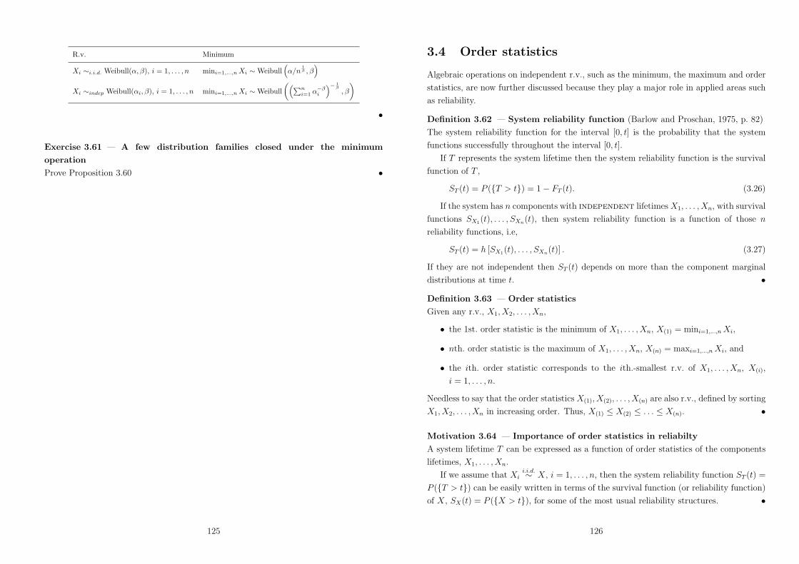
R.v. Minimum
Xi /i.i.d. Weibull(#,$), i = 1, . . . , n mini=1,...,n Xi / Weibull9#/n
1! , $
:
Xi /indep Weibull(#i, $), i = 1, . . . , n mini=1,...,n Xi / Weibull'9!n
i=1 #!"i
:! 1!
, $
(
•
Exercise 3.61 — A few distribution families closed under the minimum
operation
Prove Proposition 3.60 •
125
3.4 Order statistics
Algebraic operations on independent r.v., such as the minimum, the maximum and order
statistics, are now further discussed because they play a major role in applied areas such
as reliability.
Definition 3.62 — System reliability function (Barlow and Proschan, 1975, p. 82)
The system reliability function for the interval [0, t] is the probability that the system
functions successfully throughout the interval [0, t].
If T represents the system lifetime then the system reliability function is the survival
function of T ,
ST (t) = P ({T > t}) = 1! FT (t). (3.26)
If the system has n components with independent lifetimes X1, . . . , Xn, with survival
functions SX1(t), . . . , SXn(t), then system reliability function is a function of those n
reliability functions, i.e,
ST (t) = h [SX1(t), . . . , SXn(t)] . (3.27)
If they are not independent then ST (t) depends on more than the component marginal
distributions at time t. •
Definition 3.63 — Order statistics
Given any r.v., X1, X2, . . . , Xn,
• the 1st. order statistic is the minimum of X1, . . . , Xn, X(1) = mini=1,...,n Xi,
• nth. order statistic is the maximum of X1, . . . , Xn, X(n) = maxi=1,...,n Xi, and
• the ith. order statistic corresponds to the ith.-smallest r.v. of X1, . . . , Xn, X(i),
i = 1, . . . , n.
Needless to say that the order statistics X(1), X(2), . . . , X(n) are also r.v., defined by sorting
X1, X2, . . . , Xn in increasing order. Thus, X(1) ' X(2) ' . . . ' X(n). •
Motivation 3.64 — Importance of order statistics in reliabilty
A system lifetime T can be expressed as a function of order statistics of the components
lifetimes, X1, . . . , Xn.
If we assume that Xii.i.d./ X, i = 1, . . . , n, then the system reliability function ST (t) =
P ({T > t}) can be easily written in terms of the survival function (or reliability function)
of X, SX(t) = P ({X > t}), for some of the most usual reliability structures. •
126
Example 3.65 — Reliability function of a series system
A series system functions if all its components function. Therefore the system lifetime is
given by
T = min{X1, . . . , Xn} = X(1). (3.28)
If Xii.i.d./ X, i = 1, . . . , n, then the system reliability function is defined as
ST (t) = P
"n8
i=1
{Xi > t}$
= [SX(t)]n, (3.29)
where SX(t) = P ({X > t}). •
Exercise 3.66 — Reliability function of a series system
A series system has two components with i.i.d. lifetimes with common failure rate function
given by &X(t) = fX(t)SX(t) = 0.5t$0.5, t - 0, i.e., SX(t) = exp
G!
@ t
0 &X(s) dsH. (Prove this
result!).
Derive the system reliability function. •
Example 3.67 — Reliability function of a parallel system
A parallel system functions if at least one of its components functions. Therefore the
system lifetime is given by
T = max{X1, . . . , Xn} = X(n). (3.30)
If Xii.i.d./ X, i = 1, . . . , n, then the system reliability function equals
ST (t) = 1! FT (t)
= 1! P
"n8
i=1
{Xi ' t}$
= 1! [1! SX(t)]n , (3.31)
where SX(t) = P ({X > t}). •
Exercise 3.68 — Reliability function of a parallel system
An obsolete electronic system has 6 valves set in parallel. Assume that the components
lifetime (in years) are i.i.d. r.v. with common p.d.f. fX(t) = 50 t e$25t2 , t > 0.
Obtain the system reliability for 2 months. •
127
Proposition 3.69 — Joint p.d.f. of the order statistics and more (Murteira, 1980,
pp. 57, 55, 54)
Let X1, . . . , Xn be absolutely continuous r.v. such that Xii.i.d./ X, i = 1, . . . , n. Then:
fX(1),...,X(n)(x1, . . . , xn) = n!)
n&
i=1
fX(xi), (3.32)
for x1 ' . . . ' xn;
FX(i)(x) =
n%
j=i
'n
j
() [FX(x)]j ) [1! FX(x)]n$j
= 1! FBinomial(n,FX(x))(i! 1), (3.33)
for i = 1, . . . , n;
fX(i)(x) =
n!
(i! 1)! (n! i)!) [FX(x)]i$1 ) [1! FX(x)]n$i ) fX(x), (3.34)
for i = 1, . . . , n;
fX(i),X(j)(xi, xj) =
n!
(i! 1)! (j ! i! 1)! (n! j)!
) [FX(xi)]i$1 ) [FX(xj)! FX(xi)]
j$i$1 ) [1! FX(xj)]n$j
)fX(xi)) fX(xj), (3.35)
for xi < xj, and 1 ' i < j ' n. •
Exercise 3.70 — Joint p.d.f. of the order statistics and more
Prove Proposition 3.69 (http://en.wikipedia.org/wiki/Order statistic). •
Example 3.71 — Reliability function of a k-out-of-n system
A k-out-of-n system functions if at least k out of its n components function. A series
system corresponds to a n-out-of-n system, whereas a parallel system corresponds to a
1-out-of-n system. The lifetime of a k-out-of-n system is also associated to an order
statistic:
T = X(n$k+1). (3.36)
If Xii.i.d./ X, i = 1, . . . , n, then the system reliability function can also be derived by using
the auxiliary r.v.
Zt = number of X -is > t / Binomial(n, SX(t)). (3.37)
128

In fact,
ST (t) = P (Zt - k)
= 1! P (Zt ' k ! 1)
= 1! FBinomial(n,SX(t))(k ! 1)
= P (n! Zt ' n! k)
= FBinomial(n,FX(t))(n! k). (3.38)
•
Exercise 3.72 — Reliability function of a k-out-of-n system
Admit a machine has 4 engines and it only functions if at least 3 of those engines are
working. Moreover, suppose the lifetimes of the engines (in thousand hours) are i.i.d. r.v.
with Exponential distribution with scale parameter &$1 = 2.
Obtain the machine reliability for a period of 1000 h. •
129
3.5 Constructing independent r.v.
The following theorem is similar to Proposition 2.133 and guarantees that we can also
construct independent r.v. with prescribed d.f.
Theorem 3.73 — Construction of a finite collection of independent r.v. with
prescribed d.f. (Karr, 1993, p. 79)
Let F1, . . . , Fn be d.f. on IR. Then there is a probability space (!,F , P ) and r.v.
X1, . . . , Xn defined on it such that X1, . . . , Xn are independent r.v. and FXi = Fi for
each i. •
Exercise 3.74 — Construction of a finite collection of independent r.v. with
prescribed d.f.
Prove Proposition 3.73 (Karr, 1993, p. 79). •
Theorem 3.75 — Construction of a sequence of independent r.v. with
prescribed d.f. (Karr, 1993, p. 79)
Let F1, F2, . . . be d.f. on IR. Then there is a probability space (!,F , P ) and a r.v.
X1, X2, . . . defined on it such that X1, X2, . . . are independent r.v. and FXi = Fi for
each i. •
Exercise 3.76 — Construction of a sequence of independent r.v. with
prescribed d.f.
Prove Proposition 3.75 (Karr, 1993, pp. 79-80). •
130
3.6 Bernoulli process
Motivation 3.77 — Bernoulli (counting) process (Karr, 1993, p. 88)
Counting sucesses in repeated, independent trials, each of which has one of two possible
outcomes (success9 and failure). •
Definition 3.78 — Bernoulli process (Karr, 1993, p. 88)
A Bernoulli process with parameter p is a sequence {Xi, i " IN} of i.i.d. r.v. with Bernoulli
distribution with parameter p = P (success). •
Definition 3.79 — Important r.v. in a Bernoulli process (Karr, 1993, pp. 88–89)
In isolation a Bernoulli process is neither deep or interesting. However, we can identify
three associated and very important r.v.:
• Sn =!n
i=1 Xi, the number of successes in the first n trials (n " IN);
• Tk = min{n : Sn = k}, the time (trial number) at which the kth. success occurs
(k " IN), that is, the number of trials needed to get k successes;
• Uk = Tk!Tk$1, the time (number of trials) between the kth. and (k!1)th. successes
(k " IN, T0 = 0, U1 = T1). •
Definition 3.80 — Bernoulli counting process (Karr, 1993, p. 88)
The sequence {Sn, n " IN} is usually termed as Bernoulli counting process (or success
counting process).10 •
Exercise 3.81 — Bernoulli counting process
Simulate a Bernoulli process with parameter p = 12 and consider n = 100 trials. Plot the
realizations of both the Bernoulli process and the Bernoulli counting process. •
Definition 3.82 — Bernoulli success time process (Karr, 1993, p. 88)
The sequence {Tk, k " IN} is usually called the Bernoulli success time process. •9Or arrival.
10Sn represents the total number of successes that have occurred up to trial n, thus {Sn, n " IN}satisfies: Sn " N0, n " N; Sm ' Sn, m ' n, m, n " N; Sn ! Sm (m ' n, m, n " N) corresponds to thenumber of successes that have occurred after trial m and up to tril n. (For the continuous time analogue,see Definition 3.96.)
131
Proposition 3.83 — Important distributions in a Bernoulli process (Karr, 1993,
pp. 89–90)
In a Bernoulli process with parameter p (p " [0, 1]) we have:
• Sn / Binomial(n, p), n " IN ;
• Tk / NegativeBinomial(k, p), k " IN ;
• Uki.i.d./ Geometric(p)
d= NegativeBinomial(1, p), k " IN . •
Exercise 3.84 — Bernoulli counting process
(a) Prove that Tk / NegativeBinomial(k, p) and Uki.i.d./ Geometric(p), for k " IN .
(b) Consider a Bernoulli process with parameter p = 1/2 and obtain the probability of
having 57 successes between times 10 and 100. •
Exercise 3.85 — Relating the Bernoulli counting process and random walk
(Karr, 1993, p. 97, Exercise 3.21)
Let Sn be a Bernoulli (counting) process with p = 12 .
Prove that the process Zn = 2Sn ! n is a symmetric random walk. •
Proposition 3.86 — Properties of the Bernoulli counting process (Karr, 1993,
p. 90)
The Bernoulli counting process {Sn, n " IN} has:
• independent increments — i.e., for 0 < n1 < . . . < nk, the r.v. Sn1 , Sn2 ! Sn1 ,
Sn3 ! Sn2 , . . ., Snk! Snk!1
are independent;
• stationary increments — that is, for fixed j, the distribution of Sk+j ! Sk is the
same for all k " IN . •
Exercise 3.87 — Properties of the Bernoulli counting process
Prove Proposition 3.86 (Karr, 1993, p. 90). •
Remark 3.88 — Bernoulli counting process (web.mit.edu/6.262/www/lectures/
6.262.Lec1.pdf)
Some application areas for discrete stochastic processes such as the Bernoulli counting
process (and the Poisson process, studied in the next section) are:
132

• Operations Research
Queueing in any area, failures in manufacturing systems, finance, risk modelling,
network models
• Biology and Medicine
Epidemiology, genetics and DNA studies, cell modelling, bioinformatics, medical
screening, neurophysiology
• Computer Systems
Communication networks, intelligent control systems, data compression, detection
of signals, job flow in computer systems, physics – statistical mechanics. •
Exercise 3.89 — Bernoulli process modelling of sexual HIV transmission
(Pinkerton and Holtgrave (1998, pp. 13–14))
In the Bernoulli-process model of sexual HIV transmission, each act of sexual intercourse
is treated as an independent stochastic trial that is associated to a probability $ of HIV
transmission. $ is also known as the infectivity of HIV and a number of factors are
believed to influence $.11
(a) Prove that the expression of the probability of HIV transmission in n multiple
contacts with the same infected partner is 1! (1! $)n.
(b) Assume now that the consistent use of condoms reduce the infectivity from $ to
$- = (1! 0.9))$.12 Derive the relative change reduction in the probability defined
in (a) due to the consistent use of condoms. Evaluate this reduction when $ = 0.01
and n = 10. •
Definition 3.90 — Independent Bernoulli processes
Two Bernoulli counting processes {S(1)n , n " IN} and {S(2)
n , n " IN} are independent
if for every positive integer k and all times n1, . . . , nk, we have that the random
vector9S(1)
n1 , . . . , S(1)nk
:associated with the first process is independent of
9S(2)
n1 , . . . , S(2)nk
:
associated with the second process. •
Proposition 3.91 — Merging independent Bernoulli processes
Let {S(1)n , n " IN} and {S(2)
n , n " IN} be two independent Bernoulli counting processes
with parameters $ and ), respectively. Then the merged process {S(1)n ; S(2)
n , n " IN} is
a Bernoulli counting process with parameter $ + ) ! $).
11Such as the type of sex act engaged, sex role, etc.12## is termed reduced infectivity ; 0.9 represents a conservative estimate of condom e"ectiveness.
133
•
Exercise 3.92 — Merging independent Bernoulli processes
(a) Prove Proposition 3.91.
(b) Assume time is divided into consecutive fixed-length time-slots. Consider N sensors
and assume that the ith sensor triggers an alarm in any given fixed-length time-slot
with probability $i (i = 1, . . . , N), independently of the remaining sensors.
Obtain the probability that at least one alarm sounds in a given time-slot (Zukerman,
2000–2012, p. 60) and the p.f. of the number of times at least one alarm sounds in
the first n time-slots. •
Proposition 3.93 — Splitting a Bernoulli process (or sampling a Bernoulli
process)
Let {Sn, n " IN} be a Bernoulli counting process with parameter $. Splitting the original
Bernoulli counting process based on a selection probability p yields two Bernoulli counting
processes with parameters $p and $(1! p).
•
Exercise 3.94 — Splitting a Bernoulli process
(a) Prove Proposition 3.93.
134

Are the two resulting processes independent?13
(b) Assume once again that time is divided into consecutive fixed-length time-slots.
Moreover, assume an alarm is triggered in a fixed-length time-slot with probability $
and subsequently checked whether it is a false alarm (with probability p) or not.
Determine the p.f. of the number of time-slots between consecutive false alarms. •
13NO! If we try to merge the two splitting processes and assume they are independent we get aparameter #p + #(1! p)! #p) #(1! p) which is di"erent form #.
135
3.7 Poisson process
In what follows we use the notation of Ross (1989, Chapter 5) which is slightly di"erent
from the one of Karr (1993, Chapter 3).
Motivation 3.95 — Poisson process (Karr, 1993, p. 91)
Is there a continuous analogue of the Bernoulli process? yes!
The Poisson process, named after the French mathematician Simeon-Denis Poisson
(1781–1840), is the stochastic process in which events occur continuously and
independently of one another. Examples that are well-modeled as Poisson processes
include the radioactive decay of atoms, telephone calls arriving at a switchboard, and
page view requests to a website.14 •
Definition 3.96 — Counting process (in continuous time) (Ross, 1989, p. 209)
A stochastic process {N(t), t - 0} is said to be a counting process if N(t) represents the
total number of events (e.g. arrivals) that have occurred up to time t. From this definition
we can conclude that a counting process {N(t), t - 0} must satisfy:
• N(t) " IN0, ( t - 0;
• N(s) ' N(t), ( 0 ' s < t;
• N(t)!N(s) corresponds to the number of events that have occurred in the interval
(s, t], ( 0 ' s < t. •
Definition 3.97 — Counting process (in continuous time) with independent
increments (Ross, 1989, p. 209)
The counting process {N(t), t - 0} is said to have independent increments if the number
of events that occur in disjoint intervals are independent r.v., i.e.,
• for 0 < t1 < . . . < tn, N(t1), N(t2)!N(t1), N(t3)!N(t2), . . ., N(tn)!N(tn$1) are
independent r.v.
•
14For more examples, check http://en.wikipedia.org/wiki/Poisson process.
136

Definition 3.98 — Counting process (in continuous time) with stationary
increments (Ross, 1989, p. 210)
The counting process {N(t), t - 0} is said to have stationary increments if distribution
of the number of events that occur in any interval of time depends only on the length of
the interval,15 that is,
• N(t2 + s)!N(t1 + s)d= N(t2)!N(t1), ( s > 0, 0 ' t1 < t2. •
Definition 3.99 — Poisson process (Karr, 1993, p. 91)
A counting process {N(t), t - 0} is said to be a Poisson process with rate & (& > 0) if:
• {N(t), t - 0} has independent and stationary increments;
• N(t) / Poisson(&t). •
Remark 3.100 — Poisson process (Karr, 1993, p. 91)
Actually, N(t) / Poisson(&t) follows from the fact that {N(t), t - 0} has independent
and stationary increments, thus, redundant in Definition 3.99. •
Definition 3.101 — The definition of a Poisson process revisited (Ross, 1989, p.
212)
The counting process {N(t), t - 0} is said to be a Poisson process with rate &, if
• N(0) = 0;
• {N(t), t - 0} has independent and stationary increments;
• P ({N(h) = 1}) = &h + o(h);16
• P ({N(h) - 2}) = o(h). •
Exercise 3.102 — The definition of a Poisson process revisited
Prove that Definitions 3.99 and 3.101 are equivalent (Ross, 1989, pp. 212–214).
15The distributions do not depend on the origin of the time interval; they only depend on the lengthof the interval.
16The function f is said to be o(h) if limh$0f(h)
h = 0 (Ross, 1989, p. 211).The function f(x) = x2 is o(h) since limh$0
f(h)h = limh$0 h = 0.
The function f(x) = x is not o(h) since limh$0f(h)
h = limh$0 1 = 1 &= 0.
137
Proposition 3.103 — Joint p.f. of N(t1), . . . , N(tn) in a Poisson process (Karr,
1993, p. 91)
For 0 < t1 < . . . < tn and 0 ' k1 ' . . . ' kn,
P ({N(t1) = k1, . . . , N(tn) = kn}) =n&
j=1
e$"(tj$tj!1) [&(tj ! tj$1)]kj$kj!1
(kj ! kj$1)!, (3.39)
where t0 = 0 and k0 = 0. •
Exercise 3.104 — Joint p.f. of N(t1), . . . , N(tn) in a Poisson process
Prove Proposition 3.103 (Karr, 1993, p. 92) by taking advantage, namely, of the fact that
a Poisson process has independent and stationary increments. •
Exercise 3.105 — Joint p.f. of N(t1), . . . , N(tn) in a Poisson process (“Stochastic
Processes” — Test of 2002-11-09)
A machine produces electronic components according to a Poisson process with rate equal
to 10 components per hour. Let N(t) be the number of produced components up to time
t.
Evaluate the probability of producing at least 8 components in the first hour given
that exactly 20 components have been produced in the first two hours. •
Definition 3.106 — Important r.v. in a Poisson process (Karr, 1993, pp. 88–89)
Let {N(t), t - 0} be a Poisson process with rate &. Then:
• Sn = inf{t : N(t) = n} represents the time of the occurrence of the nth. event (e.g.
arrival), n " IN ;
• Xn = Sn ! Sn$1 corresponds to the time between the nth. and (n ! 1)th. events
(e.g. interarrival time), n " IN .
•
138
Proposition 3.107 — Important distributions in a Poisson process (Karr, 1993,
pp. 92–93)
So far we know that N(t) / Poisson(&t), t > 0. We can also add that:
• Sn / Erlang(n, &), n " IN ;
• Xni.i.d./ Exponential(&), n " IN . •
Remark 3.108 — Relating N(t) and Sn in a Poisson process
We ought to note that:
N(t) - n 2 Sn ' t (3.40)
FSn(t) = FErlang(n,")(t)
= P ({N(t) - n})
=+!%
j=n
e$"t(&t)j
j!
= 1! FPoisson("t)(n! 1), n " IN. (3.41)
•
Exercise 3.109 — Important distributions in a Poisson process
Prove Proposition 3.107 (Karr, 1993, pp. 92–93). •
Exercise 3.110 — Time between events in a Poisson process
Suppose that people immigrate into a territory at a Poisson rate & = 1 per day.
What is the probability that the elapsed time between the tenth and the eleventh
arrival exceeds two days? (Ross, 1989, pp. 216–217). •
Exercise 3.111 — Poisson process
Simulate a Poisson process with rate & = 1 considering the interval [0, 100]. Plot the
realizations of the Poisson process.
The sample path of a Poisson process should look like this:
•
139
Motivation 3.112 — Conditional distribution of the first arrival time (Ross,
1989, p. 222)
Suppose we are told that exactly one event of a Poisson process has taken place by time
t (i.e. N(t) = 1), and we are asked to determine the distribution of the time at which the
event occurred (S1). •
Proposition 3.113 — Conditional distribution of the first arrival time (Ross,
1989, p. 223)
Let {N(t), t - 0} be a Poisson process with rate & > 0. Then
S1|{N(t) = 1} / Uniform(0, t). (3.42)
•
Exercise 3.114 — Conditional distribution of the first arrival time
Prove Proposition 3.113 (Ross, 1989, p. 223). •
Proposition 3.115 — Conditional distribution of the arrival times (Ross, 1989,
p. 224)
Let {N(t), t - 0} be a Poisson process with rate & > 0. Then
fS1,...,Sn|{N(t)=n}(s1, . . . , sn) =n!
tn, (3.43)
for 0 < s1 < . . . < sn < t and n " IN . •
Remark 3.116 — Conditional distribution of the arrival times (Ross, 1989, p.
224)
Proposition 3.115 is usually paraphrased as stating that, under the condition that n events
have occurred in (0, t), the times S1, . . . , Sn at which events occur, considered as unordered
r.v., are i.i.d. and Uniform(0, t).17 •
Exercise 3.117 — Conditional distribution of the arrival times
Prove Proposition 3.115 (Ross, 1989, p. 224). •
Proposition 3.118 — Merging independent Poisson processes
Let {N1(t), t - 0} and {N2(t), t - 0} be two independent Poisson processes18 with
rates &1 and &2, respectively.
17I.e., they behave as the order statistics Y(1), . . . , Y(n), associated to Yii.i.d./ Uniform(0, t).
18How can one define two independent Poisson processes? As in Definition 3.90: two Poisson processes{N1(t), t - 0} and {N2(t), t - 0} are independent if for every positive integer k and all times t1, . . . , tk,we have that the random vector (N1(t1), . . . , N1(tk)) associated with the first process is independent of(N2(t1), . . . , N2(tk)) associated with the second process.
140

Then the merged process {N1(t)+N2(t), t - 0} is a Poisson process with rate &1 +&2.
•
Exercise 3.119 — Merging independent Poisson processes
Prove Proposition 3.118. •
Exercise 3.120 — Merging independent Poisson processes
Men and women enter a supermarket according to independent Poisson processes having
respective rates two and four per minute.
(a) Starting at an arbitrary time, compute the probability that at least two men arrive
before three women arrive (Ross, 1989, p. 242, Exercise 20).
(b) What is the probability that the number of arrivals (men and women) exceeds ten
in the first 20 minutes? •
Proposition 3.121 — Splitting a Poisson process (or sampling a Poisson
process)
Let {N(t), t - 0} be a Poisson process with rate &. Splitting the original Poisson process
based on a selection probability p yields two independent Poisson processes with rates
&p and &(1! p).
Moreover, we can add that N1(t)|{N(t) = n} / Binomial(n, p) and N2(t)|{N(t) = n} /Binomial(n, 1! p). •
141
Exercise 3.122 — Splitting a Poisson process
Prove Proposition 3.121 (Ross, 1989, pp. 218–219).
Why are the two resulting processes independent? •
Exercise 3.123 — Splitting a Poisson process
If immigrants to area A arrive at a Poisson rate of ten per week, and if each immigrant
is of English descent with probability 112 , then what is the probability that no people of
English descent will emigrate to area A during the month of February (Ross, 1989, p.
220). •
Exercise 3.124 — Splitting a Poisson process (Ross, 1989, p. 243, Exercise 23)
Cars pass a point on the highway at a Poisson rate of one per minute. If five percent of
the cars on the road are Dodges, then:
(a) What is the probability that at least one Dodge passes during an hour?
(b) If 50 cars have passed by an hour, what is the probability that five of them were
Dodges?
(c) Given that ten Dodges have passed by in an hour, obtain the expected value of the
number of cars to have passed by in that time. •
142
3.8 Generalizations of the Poisson process
In this section we consider three generalizations of the Poisson process. The first of these
is the non homogeneous Poisson process, which is obtained by allowing the arrival rate at
time t to be a function of t.
Definition 3.125 — Non homogeneous Poisson process (Ross, 1989, p. 234)
The counting process {N(t), t - 0} is said to be a non homogeneous Poisson process with
intensity function &(t) (t - 0) if
• N(0) = 0;
• {N(t), t - 0} has independent increments;
• P ({N(t + h)!N(t) = 1}) = &(t)) h + o(h), t - 0;
• P ({N(t + h)!N(t) - 2}) = o(h), t - 0.
Moreover,
N(t + s)!N(s) / Poisson
'6 t+s
s
&(z) dz
((3.44)
for s - 0 and t > 0. •
Exercise 3.126 — Non homogeneous Poisson process (“Stochastic Processes” test,
2003-01-14)
The number of arrivals to a shop is governed by a Poisson process with time dependent
rate
&(t) =
74 + 2t, 0 ' t ' 4
24! 3t, 4 < t ' 8.
(a) Obtain the expression of the expected value of the number of arrivals until t
(0 ' t ' 8). Derive the probability of no arrivals in the interval [3,5].
(b) Determine the expected value of the number of arrivals in the last 5 opening hours
(interval [3, 8]) given that 15 customers have arrived in the last 3 opening hours
(interval [5, 8]). •
143
Exercise 3.127 — The output process of an infinite server Poisson queue and
the non homogeneous Poisson process
Prove that the output process of the M/G/, queue — i.e., the number of customers who
(by time t) have already left the infinite server queue with Poisson arrivals and general
service d.f. G — is a non homogeneous Poisson process with intensity function &G(t). •
Definition 3.128 — Compound Poisson process (Ross, 1989, p. 237)
A stochastic process {X(t), t - 0} is said to be a compound Poisson process if it can be
represented as
X(t) =N(t)%
i=1
Yi, (3.45)
where
• {N(t), t - 0} is a Poisson process with rate & (& > 0) and
• Yii.i.d./ Y and independent of {N(t), t - 0}. •
Proposition 3.129 — Compound Poisson process (Ross, 1989, pp. 238–239)
Let {X(t), t - 0} be a compound Poisson process. Then
E[X(t)] = &t) E[Y ] (3.46)
V [X(t)] = &t) E[Y 2]. (3.47)
•
Exercise 3.130 — Compound Poisson process
Prove Proposition 3.129 by noting that E[X(t)] = E{E[X(t)|N(t)]} and
V [X(t)] = E{V [X(t)|N(t)]}+ V {E[X(t)|N(t)]} (Ross, 1989, pp. 238–239). •
Exercise 3.131 — Compound Poisson process (Ross, 1989, p. 239)
Suppose that families migrate to an area at a Poisson rate & = 2 per week. Assume that
the number of people in each family is independent and takes values 1, 2, 3 and 4 with
respective probabilities 16 ,
13 ,
13 and 1
6 .
What is the expected value and variance of the number of individuals migrating to
this area during a five-week period? •
144

Definition 3.132 — Conditional Poisson process (Ross, 1983, pp. 49–50)
Let:
• ( be a positive r.v. having d.f. G; and
• {N(t), t - 0} be a counting process such that, given that {( = &}, {N(t), t - 0}is a Poisson process with rate &.
Then {N(t), t - 0} is called a conditional Poisson process and
P ({N(t + s)!N(s) = n}) =
6 +!
0
e$"t(&t)n
n!dG(&). (3.48)
•
Remark 3.133 — Conditional Poisson process (Ross, 1983, p. 50)
{N(t), t - 0} is not a Poisson process. For instance, whereas it has stationary increments,
it has not independent increments. •
Exercise 3.134 — Conditional Poisson process
Suppose that, depending on factors not at present understood, the rate at which seismic
shocks occur in a certain region over a given season is either &1 or &2. Suppose also that
the rate equals &1 for p) 100% of the seasons and &2 in the remaining time.
A simple model would be to suppose that {N(t), t - 0} is a conditional Poisson
process such that ( is either &1 or &2 with respective probabilities p and 1! p.
Prove that the probability that it is a &1!season, given n shocks in the first t units of
a season, equals
p e$"1t(&1t)n
p e$"1t(&1t)n + (1! p) e$"2t(&2t)n, (3.49)
by applying the Bayes’ theorem (Ross, 1983, p. 50). •
Stochastic process Independent increments? Stationary increments?
Homogeneous PP Yes!!! Yes!!!
Non-homogeneous PP Yes!!! No!
Conditional PP No! Yes!!!
Compound PP Yes!!! Yes!!!
145
References
• Barlow, R.E. and Proschan, F. (1965/1996). Mathematical Theory of Reliability.
SIAM (Classics in Applied Mathematics).
(TA169.BAR.64915)
• Barlow, R.E. and Proschan, F. (1975). Reliability and Life Testing. Holt, Rinehart
and Winston, Inc.
• Grimmett, G.R. and Stirzaker, D.R. (2001). Probability and Random Processes
(3rd. edition). Oxford University Press. (QA274.12-.76.GRI.30385 and QA274.12-
.76.GRI.40695 refer to the library code of the 1st. and 2nd. editions from 1982 and
1992, respectively.)
• Karr, A.F. (1993). Probability. Springer-Verlag.
• Pinkerton, S.D. and Holtgrave, D.R. (1998). The Bernoulli-process model in HIV
transmission: applications and implications. In Handbook of economic evaluation
of HIV prevention programs, Holtgrave, D.R. (Ed.), pp. 13–32. Plenum Press, New
York.
• Resnick, S.I. (1999). A Probability Path. Birkhauser. (QA273.4-.67.RES.49925)
• Ross, S.M. (1983). Stochastic Processes. John Wiley & Sons. (QA274.12-
.76.ROS.36921 and QA274.12-.76.ROS.37578)
• Ross, S.M. (1989). Introduction to Probability Models (fourth edition). Academic
Press. (QA274.12-.76.ROS.43540 refers to the library code of the 5th. revised edition
from 1993.)
• Zukerman, M. (2000–2012). Introduction to Queueing Theory and Stochastic
Teletra!c Models. (arxiv.org/pdf/1307.2968)
146
Chapter 4
Expectation
One of the most fundamental concepts of probability theory and mathematical statistics
is the expectation of a r.v. (Resnick, 1999, p. 117).
Motivation 4.1 — Expectation (Karr, 1993, p. 101)
The expectation represents the center of gravity of a r.v. and has a measure theory
counterpart in integration theory.
Key computational formulas — not definitions of expectation — to obtain the
expectation of
• a discrete r.v. X with values in a countable set C and p.f. P ({X = x}) and
• the one of an absolutely continuous r.v. Y with p.d.f. fY (y)
are
E(X) =%
x"C
x) P ({X = x}) (4.1)
E(Y ) =
6 +!
$!y ) fY (y) dy, (4.2)
respectively.
When X - 0 it is permissible that E(X) = +,, but finiteness is mandatory when X
can take both positive and negative (or null) values. •
Remark 4.2 — Desired properties of expectation (Karr, 1993, p. 101)
1. Constant preserved
If X < c then E(X) = c.
147
2. Monotonicity
If X ' Y 1 then E(X) ' E(Y ).
3. Linearity
For a, b " IR, E(aX + bY ) = aE(X) + bE(Y ).
4. Continuity2
If Xn 4 X then E(Xn) 4 E(X).
5. Relation to the probability
For each event A, E(1A) = P (A).3 •
Expectation is to r.v. as probability is to events so that properties of expectation
extend those of probability.
4.1 Definition and fundamental properties
Many integration results are proved by first showing that they hold true for simple r.v.
and then extending the result to more general r.v. (Resnick, 1999, p. 117).
4.1.1 Simple r.v.
Let (!,F , P ) be a probability space and let us remind the reader that X is said to be a
simple r.v. if it assumes only finitely many values in which case
X =n%
i=1
ai ) 1Ai , (4.3)
where:
• a1, . . . , an are real numbers not necessarily distinct;
• {A1, . . . , An} constitutes a partition of !;
• 1Ai is the indicator function of event Ai, i = 1, . . . , n.
1I.e. X(!) ' Y (!),(! " !.2Continuity is not valid without restriction.3Recall that 1Ai(!) = 1, if w " Ai, and 1Ai(!) = 0, otherwise.
148
Consider, for example, X / Binomial(2, p). In this case:
• ! = {FF, FS, SF, SS} (where F = fail and S = success);
• A1 = FF , A2 = FS, A3 = SF , A4 = SS;
• a1 = 0, a2 = 1, a3 = 1, a4 = 2;
• X =!n
i=1 ai ) 1Ai .
Definition 4.3 — Expectation of a simple r.v. (Karr, 1993, p. 102)
The expectation of the simple r.v. X =!n
i=1 ai ) 1Ai is given by
E(X) =n%
i=1
ai ) P (Ai). (4.4)
•
Remark 4.4 — Expectation of a simple r.v. (Resnick, 1999, p. 119; Karr, 1993, p.
102)
• Note that Definition 4.3 coincides with our knowledge of discrete probability from
more elementary courses: the expectation is computed by taking a possible value,
multiplying by the probability of the possible value and then summing over all
possible values.
• E(X) is well-defined in the sense that all representations of X yield the same value
for E(X): di"erent representations of X, X =!n
i=1 ai)1Ai and X =!m
j=1 a-j)1A#j,
lead to the same expected value E(X) =!n
i=1 ai ) P (Ai) =!m
j=1 a-j ) P (A-j).
• The expectation of an indicator function is indeed the probability of the associated
event. •
Proposition 4.5 — Properties of the set of simple r.v. (Resnick, 1999, p. 118)
Let E be the set of all simple r.v. defined on (!,F , P ). We have the following properties
of E .
1. E is a vector space, i.e.:
(a) if X =!n
i=1 ai ) 1Ai " E and $ " IR then $X =!n
i=1 $ai ) 1Ai " E ; and
149
(b) If X =!n
i=1 ai ) 1Ai " E and Y =!m
j=1 bj ) 1Bj " E then
X + Y =n%
i=1
m%
j=1
(ai + bj)) 1Ai#Bj " E . (4.5)
2. If X, Y " E then XY " E since
XY =n%
i=1
m%
j=1
(ai ) bj)) 1Ai#Bj . (4.6)
•
Proposition 4.6 — Expectation of a linear combination of simple r.v. (Karr,
1993, p. 103)
Let X and Y be two simple r.v. and a, b " IR. Then aX + bY is also a simple r.v. and
E(aX + bY ) = aE(X) + bE(Y ). (4.7)
•
Exercise 4.7 — Expectation of a linear combination of simple r.v.
Prove Proposition 4.6 by capitalizing on Proposition 4.5 (Karr, 1993, p. 103). •
Exercise 4.8 — Expectation of a sum of discrete r.v. in a distribution problem
(Walrand, 2004, p. 51, Example 4.10.6)
Suppose you put m balls randomly in n boxes. Each box can hold an arbitrarily large
number of balls.
Prove that the expected number of empty boxes is equal to n)-
n$1n
.m. •
Exercise 4.9 — Expectation of a sum of discrete r.v. in a selection problem
(Walrand, 2004, p. 52, Example 4.10.7)
A cereal company is running a promotion for which it is giving a toy in every box of
cereal. There are n di"erent toys and each box is equally likely to contain any one of the
n toys.
Prove that the expected number of boxes of cereal you have to purchase to collect all
n toys is given by n)!n
m=11m . •
Remark 4.10 — Monotonicity of expectation for simple r.v. (Karr, 1993, p. 103)
The monotonicity of expectation for simple r.v. is a desired property which follows from
150
• linearity and
• positivity (or better said non negativity) — if X - 0 then E(X) - 0 —, a seemingly
weaker property of expectation.
In fact, if X ' Y 2 Y !X - 0 then
• E(Y )! E(X) = E(Y !X) - 0.
This argument is valid provided that E(Y )! E(X) is not of the form +,!,. •
Proposition 4.11 — Monotonicity of expectation for simple r.v. (Karr, 1993, p.
103)
Let X and Y be two simple r.v. such that X ' Y . Then E(X) ' E(Y ). •
Example 4.12 — On the (dis)continuity of expectation of simple r.v. (Karr,
1993, pp. 103–104)
Continuity of expectation fails even for simple r.v. Let P be the uniform distribution on
[0, 1] and
Xn = n) 1(0, 1n ). (4.8)
(Xn takes values: n, if ! " (0, 1n); 0, otherwise.) Then Xn(!) 4 0, (w " !, but
E(Xn) = 1, for each n.
Thus, we need additional conditions to guarantee continuity of expectation. •
151
4.1.2 Non negative r.v.
Before we proceed with the definition of the expectation of non negative r.v.,4 we need
to recall the measurability theorem. This theorem state that any non negative r.v. can
be approximated by a simple r.v., and it is the reason why it is often the case that an
integration result about non negative r.v. — such as the expectation and its properties
— is proven first to simple r.v.
Theorem 4.13 — Measurability theorem (Resnick, 1999, p. 91; Karr, 1993, p. 50)
Suppose X(!) - 0, for all !. Then X : ! 4 IR is a Borel measurable function (i.e.
a r.v.) i" there is an increasing sequence of simple and non negative r.v. X1, X2, . . .
(0 ' X1 ' X2 ' . . .) such that
Xn 5 X, (4.9)
(Xn(!) 5 X(!), for every !). •
Exercise 4.14 — Measurability theorem
Prove Theorem 4.13 by considering
Xn =n2n%
k=1
k ! 1
2n1{ k!1
2n 'X< k2n } + n) 1{X)n}, (4.10)
for each n (Resnick, 1999, p. 118; Karr, 1993, p. 50). •
Motivation 4.15 — Expectation of a non negative r.v. (Karr, 1993, pp. 103–104)
We now extend the definition of expectation to all non negative r.v. However, we have
already seen that continuity of expectation fails even for simple r.v. and therefore we
cannot define the expected value of a non negative r.v. simply as E(X) = limn&+!E(Xn).
Unsurprisingly, if we apply the measurability theorem then the definition of
expectation of a non negative r.v. virtually forces monotone continuity for increasing
sequences of non negative r.v.:
• if X1, X2, . . . are simple and non negative r.v. and X is a non negative r.v. such that
Xn 5 X (pointwise) then E(Xn) 5 E(X).
4Karr (1993) and Resnick (1999) call these r.v. positive when they are actually non negative.
152
It is convenient and useful to assume that these non negative r.v. can take values in the
extended set of non negative real numbers, IR+0 .
Further on, we shall have to establish another restricted form of continuity: dominated
continuity for integrable r.v.5 •
Definition 4.16 — Expectation of a non negative r.v. (Karr, 1993, p. 104)
The expectation of a non negative r.v. X is
E(X) = limn&+!
E(Xn) ' +,, (4.11)
where Xn are simple and non negative r.v. such that Xn 5 X.
The expectation of X over the event A is E(X; A) = E(X ) 1A). •
Remark 4.17 — Expectation of a non negative r.v. (Karr, 1993, p. 104)
The limit defining E(X)
• exists in the set of extended non negative real numbers IR+0 , and
• does not depend on the approximating sequence {Xn, n " IN}, as stated in the next
proposition. •
Proposition 4.18 — Expectation of a non negative r.v. (Karr, 1993, p. 104)
Let {Xn, n " IN} and {Xm, m " IN} be sequences of simple and non negative r.v.
increasing to X. Then
limn&+!
E(Xn) = limm&+!
E(Xm). (4.12)
•
Exercise 4.19 — Expectation of a non negative r.v.
Prove Proposition 4.18 (Karr, 1993, p. 104; Resnick, 1999, pp. 122–123). •
We now list some basic properties of the expectation operator applied to non negative
r.v. For instance, linearity, monotonicity and monotone continuity/convergence. This last
property describes how expectation and limits interact, and under which circunstances
we are allowed to interchange expectation and limits.
5We shall soon define integrable r.v.
153
Proposition 4.20 — Expectation of a linear combination of non negative r.v.
(Karr, 1993, p. 104; Resnick, 1999, p. 123)
Let X and Y be two non negative r.v. and a, b " IR+. Then
E(aX + bY ) = aE(X) + bE(Y ). (4.13)
•
Exercise 4.21 — Expectation of a linear combination of non negative r.v.
Prove Proposition 4.20 by considering two sequences of simple and non negative r.v.
{Xn, n " IN} and {Yn, n " IN} such that Xn 5 X and Yn 5 Y — and, thus, (aXn + bYn) 5(aX + bY ) — (Karr, 1993, p. 104). •
Corollary 4.22 — Monotonicity of expectation for non negative r.v. (Karr,
1993, p. 105)
Let X and Y be two non negative r.v. such that X ' Y . Then E(X) ' E(Y ). •
Remark 4.23 — Monotonicity of expectation for non negative r.v. (Karr, 1993,
p. 105)
Monotonicity of expectation follows, once again, from positivity and linearity. •
Motivation 4.24 — Fatou’s lemma (Karr, 1993, p. 105)
The next result plays a vital role in the definition of monotone continuity/convergence. •
Theorem 4.25 — Fatou’s lemma (Karr, 1993, p. 105; Resnick, 1999, p. 132)
Let {Xn, n " IN} be a sequence of non negative r.v. Then
E(lim inf Xn) ' lim inf E(Xn). (4.14)
•
Remark 4.26 — Fatou’s lemma (Karr, 1993, p. 105)
The inequality (4.14) in Fatou’s lemma can be strict. For instance, in Example 4.12 we
are dealing with E(lim inf Xn) = 0 < lim inf E(Xn) = 1. •
Exercise 4.27 — Fatou’s lemma
Prove Theorem 4.25 (Karr, 1993, p. 105; Resnick, 1999, p. 132). •
154

Exercise 4.28 — Fatou’s lemma and continuity of p.f.
Verify that Theorem 4.25 could be used in a part of the proof of the continuity of p.f. if
we considered Xn = 1An (Karr, 1993, p. 106). •
We now state another property of expectation of non negative r.v.: the monotone
continuity/convergence of expectation.
Theorem 4.29 — Monotone convergence theorem (Karr, 1993, p. 106; Resnick,
1999, pp. 123–124)
Let {Xn, n " IN} be an increasing sequence of non negative r.v. and X a non negative
r.v. If
Xn 5 X (4.15)
then
E(Xn) 5 E(X). (4.16)
•
Remark 4.30 — Monotone convergence theorem (Karr, 1993, p. 106)
The sequence of simple and non negative r.v. from Example 4.12, Xn = n ) 1(0, 1n ), does
not violate the monotone convergence theorem because in that instance it is not true that
Xn 5 X.6 •
Exercise 4.31 — Monotone convergence theorem
Prove Theorem 4.29 (Karr, 1993, p. 106; Resnick, 1999, pp. 124–125, for a more
sophisticated proof). •
Exercise 4.32 — Monotone convergence theorem and monotone continuity of
p.f.
Verify that Theorem 4.29 could be used to prove the monotone continuity of p.f. if we
considered Xn = 1An and X = 1A, where An 5 A (Karr, 1993, p. 106). •
One of the implications of the monotone convergence theorem is the linearity of
expectation for convergent series, and is what Resnick (1999, p. 131) calls the series version
of the monotone convergence theorem. This results refers under which circunstances we
are allowed to interchange expectation and limits.
6Please note that the sequence is not even increasing: n increases but the sequence of sets (0, 1n ) is a
decreasing one.
155
Theorem 4.33 — Expectation of a linear convergent series of non negative r.v.
(Karr, 1993, p. 106; Resnick, 1999, p. 131)
Let {Yk, k " IN} be a collection of non negative r.v. such that!+!
k=1 Yk(!) < +,, for
every !. Then
E
"+!%
k=1
Yk
$=
+!%
k=1
E(Yk). (4.17)
•
Exercise 4.34 — Expectation of a linear convergent series of non negative r.v.
Prove Theorem 4.33 by considering Xn =!n
k=1 Yk and applying the monotone
convergence theorem (Karr, 1993, p. 106). •
Exercise 4.35 — Expectation of a linear convergent series of non negative r.v.
and #!additivity
Verify that Theorem 4.33 could be used to prove the #!additivity of p.f. if we considered
Yk = 1Ak, where Ak are disjoint, so that
!+!k=1 Yk = 1S+$
k=1 Ak(Karr, 1993, p. 106). •
Proposition 4.36 – “Converse” of the positivity of expectation (Karr, 1993, p.
107)
Let X be a non negative r.v. If E(X) = 0 then Xa.s.= 0. •
Exercise 4.37 – “Converse” of the positivity of expectation
Prove Proposition 4.36 (Karr, 1993, p. 107). •
156
4.1.3 Integrable r.v.
It is time to extend the definition of expectation to r.v. X that can take both positive
and negative (or null) values. But first recall that:
• X+ = max{X, 0} represents the positive part of the r.v. X;
• X$ = !min{X, 0} = max{!X, 0} represents the negative part of the r.v. X;
• X = X+ !X$;
• |X| = X+ + X$.
The definition of expectation of such a r.v. preserves linearity and is based on the fact
that X can be written as a linear combination of two non negative r.v.: X = X+ !X$.
Definition 4.38 — Integrable r.v.; the set of integrable r.v. (Karr, 1993, p. 107;
Resnick, 1999, p. 126)
Let X be a r.v., not necessarily non negative. Then X is said to be integrable if
E(|X|) < +,.
The set of integrable r.v. is denoted by L1 or L1(P ) if the probability measure needs
to be emphasized. •
Definition 4.39 — Expectation of an integrable r.v. (Karr, 1993, p. 107)
Let X be an integrable r.v. Then the expectation of X is given by
E(X) = E(X+)! E(X$). (4.18)
For an event A, the expectation of X over A is E(X; A) = E(X ) 1A). •
Remark 4.40 — Expectation of an integrable r.v. (Karr, 1993, p. 107; Resnick,
1999, p. 126)
1. If X is an integrable r.v. then
E(X+) + E(X$) = E(X+ + X$) = E(|X|) < +, (4.19)
so both E(X+) and E(X$) are finite, E(X+)! E(X$) is not of the form ,!,,
thus, the definition of expectation of X is coherent.
157
2. Moreover, since |X)1A| ' |X|, E(X; A) = E(X)1A) is finite (i.e. exists!) as long
as E(|X|) < +,, that is, as long as E(X) exists.
3. Some conventions when X is not integrable...
If E(X+) < +, but E(X$) = +, then we consider E(X) = !,.
If E(X+) = +, but E(X$) < +, then we take E(X) = +,.
If E(X+) = +, and E(X$) = +, then E(X) does not exist. •
What follows refers to properties of the expectation operator.
Theorem 4.41 — Expectation of a linear combination of integrable r.v. (Karr,
1993, p. 107)
Let X and Y be two integrable r.v. — i.e., X, Y " L1 — and a, b " IR. Then aX + bY is
also an integrable r.v.7 and
E(aX + bY ) = aE(X) + bE(Y ). (4.20)
•
Exercise 4.42 — Expectation of a linear combination of integrable r.v.
Prove Theorem 4.41 (Karr, 1993, p. 108). •
Corollary 4.43 — Modulus inequality (Karr, 1993, p. 108; Resnick, 1999, p. 128)
If X " L1 then
|E(X)| ' E(|X|). (4.21)
•
Exercise 4.44 — Modulus inequality
Prove Corollary 4.43 (Karr, 1993, p. 108). •
Corollary 4.45 — Monotonicity of expectation for integrable r.v. (Karr, 1993,
p. 108; Resnick, 1999, p. 127)
If X, Y " L1 and X ' Y then
E(X) ' E(Y ). (4.22)
•
Exercise 4.46 — Monotonicity of expectation for integrable r.v.
Prove Corollary 4.45 (Resnick, 1999, pp. 127–128). •
7That is, aX + bY " L1. In fact, L1 is a vector space.
158

The continuity of expectation for integrable r.v. can be finally stated.
Theorem 4.47 — Dominated convergence theorem (Karr, 1993, p. 108; Resnick,
1999, p. 133)
Let X1, X2, . . . " L1 and X " L1 with
Xn 4 X. (4.23)
If there is a dominating r.v. Y " L1 such that
|Xn| ' Y, (4.24)
for each n, then
limn&+!
E(Xn) = E(X). (4.25)
•
Remark 4.48 — Dominated convergence theorem (Karr, 1993, p. 109)
The sequence of simple r.v., Xn = n ) 1(0, 1n ), from Example 4.12 does not violate the
dominated convergence theorem because any r.v. Y dominating Xn for each n must satisfy
Y -!+!
n=1 n ) 1( 1n+1 , 1
n ), which implies that E(Y ) = +,, thus Y &" L1 and we cannot
apply Theorem 4.47. •
Exercise 4.49 — Dominated convergence theorem
Prove Theorem 4.47 (Karr, 1993, p. 109; Resnick, 1999, p. 133, for a detailed proof). •
Exercise 4.50 — Dominated convergence theorem and continuity of p.f.
Verify that Theorem 4.47 could be used to prove the continuity of p.f. if we considered
Xn = 1An , where An 4 A, and Y < 1 as the dominating integrable r.v. (Karr, 1993, p.
109). •
4.1.4 Complex r.v.
Definition 4.51 — Integrable complex r.v.; expectation of a complex r.v. (Karr,
1993, p. 109)
A complex r.v. Z = X + iY " L1 if E(|Z|) = E(+
X2 + Y 2) < +,, and in this case the
expectation Z is E(Z) = E(X) + iE(Y ). •
159
4.2 Integrals with respect to distribution functions
Integrals (of Borel measurable functions) with respect to d.f. are known as Lebesgue–
Stieltjes integrals. Moreover, they are really expectations with respect to probabilities on
IR and are reduced to sums and Riemann (more generally, Lebesgue) integrals.
4.2.1 On integration
Remark 4.52 — Riemann integral (http://en.wikipedia.org/wiki/Riemann integral)
In the branch of mathematics known as real analysis, the Riemann integral, created
by Bernhard Riemann (1826–1866), was the first rigorous definition of the integral of a
function on an interval.
• Overview
Let g be a non-negative real-valued function of the interval [a, b], and let
S = {(x, y) : 0 < y < g(x)} be the region of the plane under the graph of the
function g and above the interval [a, b].
The basic idea of the Riemann integral is to use very simple approximations for the
area of S, denoted by@ b
a g(x) dx, namely by taking better and better approximations
— we can say that “in the limit” we get exactly the area of S under the curve.
• Riemann sums
Choose a real-valued function f which is defined on the interval [a, b]. The Riemann
sum of f with respect to the tagged partition a = x0 < x1 < x2 < . . . < xn = b
together with t0, . . . , tn$1 (where xi ' ti ' xi+1) is
n$1%
i=0
g(ti)(xi+1 ! xi), (4.26)
where each term represents the area of a rectangle with height g(ti) and length
xi+1 ! xi. Thus, the Riemann sum is the signed area under all the rectangles.
• Riemann integral
Loosely speaking, the Riemann integral is the limit of the Riemann sums of a
function as the partitions get finer.
If the limit exists then the function is said to be integrable (or more specifically
Riemann-integrable).
160

• Limitations of the Riemann integral
With the advent of Fourier series, many analytical problems involving integrals came
up whose satisfactory solution required interchanging limit processes and integral
signs.
Failure of monotone convergence — The indicator function 1Q on the rationals is not
Riemann integrable. No matter how the set [0, 1] is partitioned into subintervals,
each partition will contain at least one rational and at least one irrational number,
since rationals and irrationals are both dense in the reals. Thus, the upper Darboux
sums8 will all be one, and the lower Darboux sums9 will all be zero.
Unsuitability for unbounded intervals — The Riemann integral can only integrate
functions on a bounded interval. It can however be extended to unbounded intervals
by taking limits, so long as this does not yield an answer such as +,!,.
What about integrating on structures other than Euclidean space? — The Riemann
integral is inextricably linked to the order structure of the line. How do we free
ourselves of this limitation? •
Remark 4.53 — Lebesgue integral (http://en.wikipedia.org/wiki/Lebesgue integral;
http://en.wikipedia.org/wiki/Henri Lebesgue)
Lebesgue integration plays an important role in real analysis, the axiomatic theory of
probability, and many other fields in the mathematical sciences. The Lebesgue integral is
a construction that extends the integral to a larger class of functions defined over spaces
more general than the real line.
• Lebesgue’s theory of integration
Henri Leon Lebesgue (1875–1941) invented a new method of integration to solve
this problem. Instead of using the areas of rectangles, which put the focus on the
domain of the function, Lebesgue looked at the codomain of the function for his
fundamental unit of area. Lebesgue’s idea was to first build the integral for what he
called simple functions, measurable functions that take only finitely many values.
Then he defined it for more complicated functions as the least upper bound of all
the integrals of simple functions smaller than the function in question.
8The upper Darboux sum of g with respect to the partition is!n!1
i=0 (xi+1 ! xi)Mi+1, whereMi+1 = supx%[xi,xi+1] g(x).
9The lower Darboux sum of g with respect to the partition is!n
i=0(xi+1 ! xi)mi+1, wheremi+1 = infx%[xi,xi+1] g(x).
161
Lebesgue integration has the beautiful property that every bounded function defined
over a bounded interval with a Riemann integral also has a Lebesgue integral, and
for those functions the two integrals agree. But there are many functions with a
Lebesgue integral that have no Riemann integral.
As part of the development of Lebesgue integration, Lebesgue invented the concept
of Lebesgue measure, which extends the idea of length from intervals to a very large
class of sets, called measurable sets.
• Integration
We start with a measure space (!,F , µ) where ! is a set, F is a # ! algebra of
subsets of ! and µ is a (non-negative) measure on F of subsets of !.
In the mathematical theory of probability, we confine our study to a probability
measure µ, which satisfies µ(!) = 1.
In Lebesgue’s theory, integrals are defined for a class of functions called measurable
functions.
We build up an integral@
# g dµ for measurable real-valued functions g defined on !
in stages:
– Indicator functions. To assign a value to the integral of the indicator
function of a measurable set S consistent with the given measure µ, the only
reasonable choice is to set6
#
1S dµ = µ(S).
– Simple functions. A finite linear combination of indicator functions!
k ak1Sk. When the coe$cients ak are non-negative and Sk are disjoint sets
of !, we set6
#
(%
k
ak1Sk) dµ =
%
k
ak
6
#
1Skdµ =
%
k
ak µ(Sk).
– Non-negative functions. We define6
#
g dµ = sup
L 6
#
s dµ : 0 ' s ' g, s simple
M.
– Signed functions. g = g+ ! g$... And it makes sense to define6
#
gdµ =
6
#
g+dµ!6
#
g$dµ.
•
162

Remark 4.54 — Lebesgue/Riemann–Stieltjes integration
(http://en.wikipedia.org/wiki/Lebesgue-Stieltjes integration)
The Lebesgue–Stieltjes integral is the ordinary Lebesgue integral with respect to a measure
known as the Lebesgue–Stieltjes measure, which may be associated to any function of
bounded variation on the real line.
• Definition
The Lebesgue–Stieltjes integral@ b
a g(x) dF (x) is defined when g : [a, b] 4 IR is Borel-
measurable and bounded and F : [a, b] 4 IR is of bounded variation in [a, b] and
right-continuous, or when g is non-negative and F is monotone and right-continuous.
• Riemann–Stieltjes integration and probability theory
When g is a continuous real-valued function of a real variable and F is a
non-decreasing real function, the Lebesgue–Stieltjes integral is equivalent to the
Riemann–Stieltjes integral, in which case we often write@ b
a g(x) dF (x) for the
Lebesgue–Stieltjes integral, letting the measure PF remain implicit.
This is particularly common in probability theory when F is the cumulative
distribution function of a real-valued random variable X, in which case6 !
$!g(x) dF (x) = EF [g(X)].
•
4.2.2 Generalities
First of all, we should recall that given a d.f. F on IR, there is a unique p.f. on IR such
that PF ((a, b]) = F (b)! F (a).
Moreover, all functions g appearing below are assumed to be Borel measurable.
Definition 4.55 — Integral of a nonnegative g with respect to a d.f. (Karr, 1993,
p. 110)
Let F be a d.f. on IR and g a non negative function. Then the integral of g with respect
to F is given by6
IR
g(x) dF (x) = EF (g) ' +,, (4.27)
where the expectation is that of g(X) as a Borel measurable function of the r.v. X defined
on the probability space (IR,B(IR), PF ). •
163
Definition 4.56 — Integrable of a function with respect to a d.f. (Karr, 1993, p.
110)
Let F be a d.f. on IR and g a signed function. Then g is said to be integrable with respect
to F if@
IR g(x) dF (x) < +,, and in this case, the integral of g with respect to F equals6
IR
g(x) dF (x) =
6
IR
g+(x) dF (x)!6
IR
g$(x) dF (x). (4.28)
•
Definition 4.57 — Integral of a function over a set with respect to a d.f. (Karr,
1993, p. 110)
Let F be a d.f. on IR and g either non negative or integrable and B " B(IR). The integral
of g over B with respect to F is equal to6
B
g(x) dF (x) =
6
IR
g(x)) 1B(x) dF (x). (4.29)
•
The properties of the integral of a function with respect to a d.f. are those of
expectation:
1. Constant preserved
2. Monotonicity
3. Linearity
4. Relation to PF
5. Fatou’s lemma
6. Monotone convergence theorem
7. Dominated convergence theorem
164
4.2.3 Discrete distribution functions
Keep in mind that integrals with respect to discrete d.f. are sums.
Theorem 4.58 — Integral with respect to a discrete d.f. (Karr, 1993, p. 111)
Consider a d.f. F (t) that can be written as
F (x) =%
i
pi ) 1[xi,+!)(x). (4.30)
Then, for each g - 0,6
IR
g(x) dF (x) =%
i
g(xi)) pi. (4.31)
•
Exercise 4.59 — Integral with respect to a discrete d.f.
Prove Theorem 4.58 (Karr, 1993, p. 111). •
Corollary 4.60 — Integrable function with respect to a discrete d.f. (Karr, 1993,
p. 111)
The function g is said to be integrable with respect to the discrete d.f. F i"%
i
|g(xi)|) pi < +,, (4.32)
and in this case6
IR
g(x) dF (x) =%
i
g(xi)) pi. (4.33)
•
4.2.4 Absolutely continuous distribution functions
Now note that integrals with respect to absolutely continuous d.f. are Riemann integrals.
Theorem 4.61 — Integral with respect to an absolutely continuous d.f. (Karr,
1993, p. 112)
Suppose that the d.f. F is absolutely continuous and is associated to a piecewise continuous
p.d.f. f . If g is a non negative function and piecewise continuous then6
IR
g(x) dF (x) =
6 +!
$!g(x)) f(x) dx, (4.34)
where the integral on the right-hand side is an improper Riemann integral. •
165
Exercise 4.62 — Integral with respect to an absolutely continuous d.f.
Prove Theorem 4.61 (Karr, 1993, p. 112). •
Corollary 4.63 — Integral with respect to an absolutely continuous d.f. (Karr,
1993, p. 112)
A piecewise continuous function g is said to be integrable with respect to the d.f. F i"6 +!
$!|g(x)|f(x) dx < +,, (4.35)
and in this case6
IR
g(x) dF (x) =
6 +!
$!g(x)) f(x) dx. (4.36)
•
4.2.5 Mixed distribution functions
Recall that a mixed d.f. F is a convex combination of a discrete d.f.
Fd(x) =%
i
pi ) 1[xi,+!)(x) (4.37)
and an absolutely continuous d.f.
Fa(x) =
6 x
$!fa(s) ds. (4.38)
Thus,
F (x) = $) Fd(x) + (1! $)) Fa(x), (4.39)
where $ " (0, 1).
Corollary 4.64 — Integral with respect to a mixed d.f. (Karr, 1993, p. 112)
The integral of g with respect to the mixed d.f. F is a corresponding combination of
integrals with respect to Fd and Fa:6
IR
g(x) dF (x) = $)6
IR
g(x) dFd(x) + (1! $))6
IR
g(x) dFa(x)
= $)%
i
g(xi)) pi + (1! $))6 +!
$!g(x)) fa(x) dx. (4.40)
In order that the integral with respect to a mixed d.f. exists, g must be piecewise
continuous and either non negative or integrable with respect to both Fd and Fa. •
166

4.3 Computation of expectations
So far we have defined the expectation for simple r.v.
The expectations of other types of r.v. — such as non negative, integrable and mixed
r.v. — naturally involve integrals with respect to distribution functions.
4.3.1 Non negative r.v.
The second equality in the next formula is quite convenient because it allows us to obtain
the expectation of a non negative r.v. — be it a discrete, absolutely continuous or mixed
— in terms of an improper Riemann integral.
Theorem 4.65 — Expected value of a non negative r.v. (Karr, 1993, p. 113)
If X - 0 then
E(X) =
6 +!
0
x dFX(x) =
6 +!
0
[1! FX(x)] dx. (4.41)
•
Exercise 4.66 — Expected value of a non negative r.v.
Prove Theorem 4.65 (Karr, 1993, pp. 113–114). •
Corollary 4.67 — Expected value of a non negative integer-valued r.v. (Karr,
1993, p. 114)
Let X be a non negative integer-valued r.v. Then
E(X) =+!%
n=1
n) P ({X = n}) =+!%
n=1
P ({X - n}) =+!%
n=0
P ({X > n}). (4.42)
•
Exercise 4.68 — Expected value of a non negative integer-valued r.v.
Prove Corollary 4.67 (Karr, 1993, p. 114). •
Corollary 4.69 — Expected value of a non negative absolutely continuous r.v.
Let X be a non negative absolutely continuous r.v. with p.d.f. fX(x).
E(X) =
6 +!
0
x) fX(x) dx =
6 +!
0
[1! FX(x)] dx. (4.43)
•
167
Exercise 4.70 — A nonnegative r.v. with infinite expectation
Let X / Pareto(b = 1, $ = 1). i.e.
fX(x) =
7% b"
x"+1 = 1x2 , x - b = 1
0, otherwise.(4.44)
Prove that E(X) exists and E(X) = +, (Resnick, 1999, p. 126, Example 5.2.1). •
4.3.2 Integrable r.v.
Let us remind the reader that X is said to be an integrable r.v. if E(|X|) = E(X+) +
E(X$) < +,.
Theorem 4.71 — Expected value of an integrable r.v. (Karr, 1993, p. 114)
If X is an integrable r.v. then
E(X) =
6 +!
$!x dFX(x). (4.45)
•
Exercise 4.72 — Expected value of an integrable r.v.
Prove Theorem 4.71 (Karr, 1993, p. 114). •
Corollary 4.73 — Expected value of an integrable discrete or absolutely
continuous r.v.
Let X be an integrable discrete or absolutely continuous r.v. with p.f. P (X = x) or p.d.f.
fX(x) then
E(X) =%
x
x) P (X = x) dx (4.46)
E(X) =
6 +!
$!x) fX(x) dx, (4.47)
respectively. •
Exercise 4.74 — Real r.v. without expectation
After having derived the c.d.f. of X+ and X$, use Theorem 4.65 to prove that E(X+) =
E(X$) = +, — and therefore E(X) does not exist — if X has p.d.f. equal to:
(a) fX(x) =
71
2x2 , |x| > 1
0, otherwise;
168

(b) fX(x) =1
"(1 + x2), x " IR.
(Resnick, 1999, p. 126, Example 5.2.1.)10 •
4.3.3 Mixed r.v.
When dealing with mixed r.v. X we take advantage of the fact that FX(x) is a convex
combination of the d.f. of a discrete r.v. Xd and the d.f. of an absolutely continuous r.v.
Xa.
Corollary 4.75 — Expectation of a mixed r.v.
The expected value of the mixed r.v. X with d.f. FX(x) = $)FXd(x)+ (1!$))FXa(x),
where $ " (0, 1), is given by6
IR
x dFX(x) = $)6
IR
x dFXd(x) + (1! $))
6
IR
x dFXa(x)
= $)%
i
xi ) P ({Xd = xi})
+(1! $))6 +!
$!x) fXa(x) dx (4.48)
= $ E(Xd) + (1! $) E(Xa). (4.49)
•Exercise 4.76 — Expectation of a mixed r.v.
A random variable X has the following d.f.:11
FX(x) =
)***+
***,
0, x < 0
0.3, 0 ' x < 2
0.3 + 0.2x, 2 ' x < 3
1, x - 3.
(4.50)
(a) Why is X a mixed r.v.?
(b) Write FX(x) as a linear combination of the d.f. of two r.v.: a discrete and an
absolutely continuous r.v.
(c) Obtain the expected value of X, by using the fact that X is non negative, thus,
E(X) =@ +!
0 [1! FX(x)] dx.
Compare this value with the one you would obtain using Corollary 4.75. •
10There is a typo in the definition of the first p.d.f. in Resnick (1999): x > 1 should read as |x| > 1.The second p.d.f. corresponds to the one of a r.v. with (standard) Cauchy distribution.
11Adapted from Walrand (2004, pp. 53–55, Example 4.10.9).
169
Exercise 4.77 — Expectation of a mixed r.v. in a queueing setting
Consider a M/M/1 system.12 Let:
• Ls be the number of customers an arriving customer finds in the system in
equilibrium;13
• Wq be the waiting time in queue of this arriving customer.14
Under these conditions, we can state that
P (Ls = k) = (1! ()) (k, k " IN0; (4.51)
thus, Ls / geometric,(1! (), where ( = "µ " (0, 1) and E(Ls) = $
1$$ .
(a) Argue that Wq|{Ls = k} / Gamma(k, µ), for k " IN .
(b) Prove that Wq|{Wq > 0} / Exponential(µ(1! ()).
(c) Demonstrate that Wq is a mixed r.v. with d.f. given by:
FWq(w) =
70, w < 0
(1! () + () FExp(µ(1$$))(w), w - 0.(4.52)
(d) Verify that E(Wq) = $µ(1$$) . •
12The arrivals to the system are governed by a Poisson process with rate ", i.e. the time between arrivalshas an exponential distribution with parameter "; needless to say, M stands for memoryless. The servicetimes are not only i.i.d. with exponential distribution with parameter µ, but also independent from thearrival process. There is only one server, and the service policy is FCFS (first come first served). & = #
µ
represents the tra$c intensity and we assume that & " (0, 1).13Equilibrium roughly means that a lot of time has elapsed since the system has been operating and
therefore the initial conditions no longer influence the state of system.14Wq is the time elapsed from the moment the customer arrives until his/her service starts in the
system in equilibrium.
170
4.3.4 Functions of r.v.
Unsurprisingly, we are surely able to derive expressions for the expectation of a Borel
measurable function g of the r.v. X, E[g(X)]. Obtaining this expectation does not require
the derivation of the d.f. of g(X) and follows from section 4.2.
In the two sections we shall discuss the expectation of specific functions of r.v.:
g(X) = Xk, k " IN .
Theorem 4.78 — Expected value of a function of a r.v. (Karr, 1993, p. 115)
Let X be a r.v., and g be a Borel measurable function either non negative or integrable.
Then
E[g(X)] =
6
IR
g(x) dFX(x). (4.53)
•
Exercise 4.79 — Expected value of a function of a r.v.
Prove Theorem 4.78 (Karr, 1993, p. 115). •
Corollary 4.80 — Expected value of a function of a discrete r.v. (Karr, 1993, p.
115)
Let X be a discrete r.v., and g be a Borel measurable function either non negative or
integrable. Then
E[g(X)] =%
xi
g(xi)) P ({X = xi}). (4.54)
•
Corollary 4.81 — Expected value of a function of an absolutely continuous r.v.
(Karr, 1993, p. 115)
Let X be an absolutely continuous r.v., and g be a Borel measurable function either non
negative or integrable. Then
E[g(X)] =
6 +!
$!g(x)) fX(x) dx. (4.55)
•
171
4.3.5 Functions of random vectors
When dealing with functions of random vectors, the only useful formulas are those
referring to the expectation of functions of discrete and absolutely continuous random
vectors.
These formulas will be used to obtain, for instance, what we shall call measures of
(linear) association between r.v.
Theorem 4.82 — Expectation of a function of a discrete random vector (Karr,
1993, p. 116)
Let:
• X1, . . . , Xd be a discrete r.v., with values in the countable sets C1, . . . , Cd,
respectively;
• g : IRd 4 IR be a Borel measurable function either non negative or integrable (i.e.
g(X1, . . . , Xd) " L1).
Then
E[g(X1, . . . , Xd)] =%
x1"C1
. . .%
xd"Cd
g(x1, . . . , xd)) P ({X1 = x1, . . . , Xd = xd}).(4.56)
•
Theorem 4.83 — Expectation of a function of an absolutely continuous
random vector (Karr, 1993, p. 116)
Let:
• (X1, . . . , Xd) be an absolutely continuous random vector with joint p.d.f.
fX1,...,Xd(x1, . . . , xd);
• g : IRd 4 IR be a Borel measurable function either non negative or integrable.
Then
E[g(X1, . . . , Xd)]
=
6 +!
$!. . .
6 +!
$!g(x1, . . . , xd)) fX1,...,Xd
(x1, . . . , xd) dx1 . . . dxd. (4.57)
•
Exercise 4.84 — Expectation of a function of an absolutely continuous random
vector
Prove Theorem 4.83 (Karr, 1993, pp. 116–117). •
172
4.3.6 Functions of independent r.v.
When all the components of the random vector (X1, . . . , Xd) are independent, the formula
of E[g(X1, . . . , Xd)] can be simplified.
The next results refer to two independent random variables (d = 2). The generalization
for d > 2 is straightforward.
Theorem 4.85 — Expectation of a function of two independent r.v. (Karr, 1993,
p. 117)
Let:
• X and Y be two independent r.v.
• g : IR2 4 IR+ be a Borel measurable non negative function.
Then
E[g(X, Y )] =
6
IR
I6
IR
g(x, y) dFX(x)
JdFY (y)
=
6
IR
I6
IR
g(x, y) dFY (y)
JdFX(x). (4.58)
•
Moreover, the expectation of the product of functions of independent r.v. is the product
of their expectations. Also note that the product of two integrable r.v. need not be
integrable.
Corollary 4.86 — Expectation of a function of two independent r.v. (Karr,
1993, p. 118)
Let:
• X and Y be two independent r.v.
• g1, g2 : IR 4 IR be two Borel measurable functions either non negative or integrable.
Then g1(X)) g2(Y ) is integrable and
E[g1(X)) g2(Y )] = E[g1(X)]) E[g2(Y )]. (4.59)
•
Exercise 4.87 — Expectation of a function of two independent r.v.
Prove Theorem 4.85 (Karr, 1993, p. 117) and Corollary 4.86 (Karr, 1993, p. 118). •
173
4.3.7 Sum of independent r.v.
We are certainly not going to state that E(X + Y ) = E(X) + E(Y ) when X and Y are
simple or non negative or integrable independent r.v.15
Instead, we are going to write the d.f. of the sum of two independent r.v. in terms
of integrals with respect to the d.f. and define a convolution of d.f.16
Theorem 4.88 — D.f. of a sum of two independent r.v. (Karr, 1993, p. 118)
Let X and Y be two independent r.v. Then
FX+Y (t) =
6
IR
FX(t! y) dFY (y) =
6
IR
FY (t! x) dFX(x). (4.60)
•
Exercise 4.89 — D.f. of a sum of two independent r.v.
Prove Theorem 4.88 (Karr, 1993, p. 118). •
Corollary 4.90 — D.f. of a sum of two independent discrete r.v.
Let X and Y be two independent discrete r.v. Then
FX+Y (t) =%
y
FX(t! y)) P ({Y = y}) =%
x
FY (t! x)) P ({X = x}). (4.61)
•
Remark 4.91 — D.f. of a sum of two independent discrete r.v.
The previous formula is not preferable to the one we derived for the p.f. of X + Y in
Chapter 2 because it depends in fact on two sums... •
Corollary 4.92 — D.f. of a sum of two independent absolutely continuous r.v.
Let X and Y be two independent absolutely continuous r.v. Then
FX+Y (t) =
6 +!
$!FX(t! y)) fY (y) dy =
6 +!
$!FY (t! x)) fX(x) dx. (4.62)
•
Let us revisit an exercise from Chapter 2 to illustrate the use of Corollary 4.92.
15This result follows from the linearity of expectation.16Recall that in Chapter 2 we derived expressions for the p.f. and the p.d.f. of the sum of two
independent r.v.
174

Exercise 4.93 — D.f. of the sum of two independent absolutely continuous r.v.
Let X and Y be the durations of two independent system components set in what is called
a stand by connection.17 In this case the system duration is given by X + Y .
(a) Derive the d.f. of X + Y , assuming that X / Exponencial($) and Y /Exponencial()), where $, ) > 0 and $ &= ), and using Corollary 4.92.
(b) Prove that the associated p.d.f. equals fX+Y (z) =%&(e!%z$e!"z)
%$& , z > 0. •
Definition 4.94 — Convolution of d.f. (Karr, 1993, p. 119)
Let X and Y be independent r.v. Then
(FX , FY )(t) = FX+Y (t) =
6
IR
FX(t! y) dFY (y) =
6
IR
FY (t! x) dFX(x) (4.63)
is said to be the convolution of the d.f. FX and FY . •
17At time 0, only the component with duration X is on. The component with duration Y replaces theother one as soon as it fails.
175
4.4 Lp spaces
Motivation 4.95 — Lp spaces (Karr, 1993, p. 119)
While describing a r.v. in a partial way, we tend to deal with E(Xp), p " [1, +,), or a
function of several such expected values. Needless to say that we have to guarantee that
E(|X|p) is finite. •
Definition 4.96 — Lp spaces (Karr, 1993, p. 119)
The space Lp, for a fixed p " [1, +,), consists of all r.v. X whose pth absolute power is
integrable, that is,
E(|X|p) < +,. (4.64)
•
Exercise 4.97 — Exponential distributions and Lp spaces
Let X / Exponential(&), & > 0.
Prove that X " Lp, for any p " [1, +,). •
Exercise 4.98 — Pareto distributions and Lp spaces
Let X / Pareto(b, $) i.e.
fX(x) =
7% b"
x"+1 , x - b
0, otherwise(4.65)
where b > 0 is the minimum possible value of X and $ > 0 is called the Pareto index.
For which values of p " [1, +,) we have X " Lp? •
176

4.5 Key inequalities
What immediately follows is a table with an overview of a few extremely useful inequalities
involving expectations.
Some of these inequalities are essential to prove certain types of convergence of
sequences of r.v. in Lp and uniform integrability (Resnick, 1999, p. 189)18 and provide
answers to a few questions we compiled after the table.
Finally, we state and treat each inequality separately.
Proposition 4.99 — A few (moment) inequalities (Karr, 1993, p. 123;
http://en.wikipedia.org)
(Moment) inequality Conditions Statement of the inequality
Young h : IR+0 & IR+
0 continuous, strictly increasing, a/ b ' H(a) + K(b)
h(0) = 0, h(+!) = +!, H(x) =R x0 h(y) dy
k pointwise inverse of h, K(x) =R x0 k(y) dy
a, b " IR+
Holder X " Lp, Y " Lq , E(|X / Y |) ' E1p (|X|p)/ E
1q (|Y |q)
where p, q " [1, +!) : 1p + 1
q = 1 (X / Y " L1)
Cauchy-Schwarz X, Y " L2 E(|X / Y |) 'p
E(X2)/ E(Y 2)
(X / Y " L1)
Liapunov X " Ls, 1 ' r ' s E1r (|X|r) ' E
1s (|X|s)
(Ls 1 Lr)
Minkowski X, Y " Lp, p " [1, +!) E1p (|X + Y |p) ' E
1p (|X|p) + E
1p (|Y |p)
(X + Y " Lp)
Jensen g convex; X, g(X) " L1 g[E(X)] ' E[g(X)]
g concave; X, g(X) " L1 g[E(X)] ) E[g(X)]
Chebyshev X ) 0, P ({X ) a}) ' E[g(X)]g(a)
g non negative and increasing, a > 0
(Cherno$) X ) 0, a, t > 0 P ({X ) a}) ' E(etX )eta
(Markov) X " L1, a > 0 P ({|X| ) a}) ' E[|X|]a ;
X " Lp, a > 0 P ({|X| ) a}) ' E[|X|p]ap
(Chebyshev-Bienayme) X " L2, a > 0 P ({|X $ E(X)| ) a}) ' V (X)a2
X " L2, a > 0 P“n
|X $ E(X)| ) ap
V (X)o”
' 1a2
(Cantelli) X " L2, a > 0 P ({|X $ E(X)| ) a}) ' 2V (X)a2+V (X)
(one-sided Chebyshev) X " L2, a > 0 P“n
X $ E(X) ) ap
V (X)o”
' 11+a2
•
18For a definition of uniform integrability see http://en.wikipedia.org/wiki/Uniform integrability.
177
Motivation 4.100 — A few (moment) inequalities
• Young — How can we relate the areas under (resp. above) an increasing function h
in the interval [0, a] (resp. in the interval of [0, h$1(b)]) with the area of the rectangle
with vertices (0, 0), (0, b), (a, 0) and (a, b), where b " (0, maxx"[0,a] h(x)]?
• Holder/Cauchy-Schwarz — What are the su$cient conditions on r.v. X and Y
to be dealing with an integrable product XY ?
• Liapunov — What happens to the spaces Lp when p increases in [1, +,)? Is it a
decreasing (increasing) sequence of sets?
What happens to the norm of a r.v. in Lp, ||X||p = E1p (|X|p)? Is it an increasing
(decreasing) function of p " [1, +,)?
• Minkowski — What are the su$cient conditions on r.v. X and Y to be dealing
with a sum X + Y " Lp? Is Lp a vector space?
• Jensen — Under what conditions we can relate g[E(X)] and E[g(X)]?
• Chebyshev — When can we provide non trivial upper bounds for the tail
probability P ({X - a}) •
4.5.1 Young’s inequality
The first inequality (not a moment inequality) is named after William Henry Young
(1863–1942), an English mathematician, and can be used to prove Holder inequality.
Lemma 4.101 — Young’s inequality (Karr, 1993, p. 119)
Let:
• h : IR+0 4 IR+
0 be a continuous and strictly increasing function such that h(0) = 0,
h(+,) = +,;
• k be the pointwise inverse of h;
• H(x) =@ x
0 h(y) dy be the area under h in the interval [0, x];
• K(x) =@ x
0 k(y) dy be the area above h in the interval [0, h$1(x)] = [0, k(x)];
• a, b " IR+.
Then
a) b ' H(a) + K(b). (4.66)•
178
Exercise 4.102 — Young’s inequality (Karr, 1993, p. 119)
Prove Lemma 4.101, by using a graphical argument (Karr, 1993, p. 119). •
Remark 4.103 — A special case of Young’s inequality
If we apply Young’s inequality to h(x) = xp$1, p " [1, +,) and consider
• a and b non negative real numbers,
• q = 1 + 1p$1 " [1, +,) i.e. 1
p + 1q = 1,
then
a) b ' ap
p+
bq
q. (4.67)
For the proof of this result see http://en.wikipedia.org/wiki/Young’s inequality, which
states (4.67) as Young’s inequality. See also Karr (1993, p. 120) for a reference to (4.67)
as a consequence of Young’s inequality as stated in (4.66). •
4.5.2 Holder’s moment inequality
In mathematical analysis Holder’s inequality, named after the German mathematician
Otto Holder (1859–1937), is a fundamental inequality between integrals, an indispensable
tool for the study of Lp spaces and essential to prove Liapunov’s and Minkowski’s
inequalities.
Interestingly enough, Holder’s inequality was first found by the British mathematician
L.J. Rogers (1862–1933) in 1888, and discovered independently by Holder in 1889.
Theorem 4.104 — Holder’s moment inequality (Karr, 1993, p. 120)
Let
• X " Lp, Y " Lq, where p, q " [1, +,) : 1p + 1
q = 1.
Then
X ) Y " L1 (4.68)
E(|XY |) ' E1p (|X|p)) E
1q (|Y |q). (4.69)
•
179
Remarks 4.105 — Holder’s (moment) inequality
• The numbers p and q above are said to be Holder conjugates of each other.
• For the detailed statement of Holder inequality in measure spaces, check
http://en.wikipedia.org/wiki/Holder’s inequality. Two notable special cases
follow...
• In case we are dealing with S, a measurable subset of IR with the Lebesgue measure,
and f and g are measurable real-valued functions on S then Holder’s inequality reads
as follows:
6
S
|f(x)) g(x)| dx ''6
S
|f(x)|p dx
( 1p
)'6
S
|g(x)|q dx
( 1q
. (4.70)
• When we are dealing with n!dimensional Euclidean space and the counting
measure, we have
n%
k=1
|xk ) yk| '"
n%
k=1
|xk|p$ 1
p
)"
n%
k=1
|yk|q$ 1
q
, (4.71)
for all (x1, . . . , xn), (y1, . . . , yn) " IRn.
• For a generalization of Holder’s inequality involving n (instead of 2) Holder
conjugates, see http://en.wikipedia.org/wiki/Holder’s inequality. •
Exercise 4.106 — Holder’s moment inequality
Prove Theorem 4.104, by using the special case of Young’s inequality (4.67), considering
a = |X|
E1p (|X|p)
and b = |Y |
E1q (|Y |q)
, taking expectations to (4.67), and applying the result
1p + 1
q = 1 (Karr, 1993, p. 120). •
180

4.5.3 Cauchy-Schwarz’s moment inequality
A special case of Holder’s moment inequality — p = q = 2 — is nothing but the Cauchy-
Schwarz’s moment inequality.
In mathematics, the Cauchy-Schwarz inequality19 is a useful inequality encountered
in many di"erent settings, such as linear algebra applied to vectors, in analysis applied to
infinite series and integration of products, and in probability theory, applied to variances
and covariances.
The inequality for sums was published by Augustin Cauchy in 1821, while the
corresponding inequality for integrals was first stated by Viktor Yakovlevich Bunyakovsky
in 1859 and rediscovered by Hermann Amandus Schwarz in 1888 (often misspelled
“Schwartz”).
Corollary 4.107 — Cauchy-Schwarz’s moment inequality (Karr, 1993, p. 120)
Let X, Y " L2. Then
X ) Y " L1 (4.72)
E(|X ) Y |) 'K
E(|X|2)) E(|Y |2). (4.73)
•
Remarks 4.108 — Cauchy-Schwarz’s moment inequality
(http://en.wikipedia.org/wiki/Cauchy-Schwarz inequality)
• In the Euclidean space IRn with the standard inner product, the Cauchy-Schwarz’s
inequality is
"n%
i=1
xi ) yi
$2
'"
n%
i=1
x2i
$)
"n%
i=1
y2i
$. (4.74)
• The triangle inequality for the inner product is often shown as a consequence of the
Cauchy-Schwarz inequality, as follows: given vectors x and y, we have
=x + y=2 = >x + y, x + y?' (=x=+ =y=)2 . (4.75)
•19Also known as the Bunyakovsky inequality, the Schwarz inequality, or the Cauchy-Bunyakovsky-
Schwarz inequality (http://en.wikipedia.org/wiki/Cauchy-Schwarz inequality).
181
Exercise 4.109 — Confronting the squared covariance and the product of the
variance of two r.v.
Prove that
|cov(X, Y )|2 ' V (X)) V (Y ), (4.76)
where X, Y " L2 (http://en.wikipedia.org/wiki/Cauchy-Schwarz’s inequality). •
4.5.4 Lyapunov’s moment inequality
The spaces Lp decrease as p increases in [1, +,). Moreover, E(|X|p)1p is an increasing
function of p " [1, +,).
The following moment inequality is a special case of Holder’s inequality and is due to
Aleksandr Mikhailovich Lyapunov (1857–1918), a Russian mathematician, mechanician
and physicist.20
Corollary 4.110 — Lyapunov’s moment inequality (Karr, 1993, p. 120)
Let X " Ls, where 1 ' r ' s. Then
Ls 3 Lr (4.77)
E1r (|X|r) ' E
1s (|X|s). (4.78)
•Remarks 4.111 — Lyapunov’s moment inequality
• Taking s = 2 and r = 1 we can conclude that
E2(|X|) ' E(X2). (4.79)
This result is not correctly stated in Karr (1993, p. 121) and can be also deduced
from the Cauchy-Schwarz’s inequality, as well as from Jensen’s inequality, stated
below.
• Rohatgi (1976, p. 103) states Liapunov’s inequality in a slightly di"erent way. It
can be put as follows: for X " Lk, k " [1, +,),
E1k (|X|k) ' E
1k+1 (|X|k+1). (4.80)
20Lyapunov is known for his development of the stability theory of a dynamical system,as well as for his many contributions to mathematical physics and probability theory(http://en.wikipedia.org/wiki/Aleksandr Lyapunov).
182

• The equality in (4.78) holds i" X is a degenerate r.v., i.e. Xd= c, where c is a real
constant (Rohatgi, 1976, p. 103). •
Exercise 4.112 — Lyapunov’s moment inequality
Prove Corollary 4.110, by applying Holder’s inequality to X - = Xr, where X " Lr, and
to Yd= 1, and considering p = s
r (Karr, 1993, pp. 120–121).21 •
4.5.5 Minkowski’s moment inequality
The Minkowski’s moment inequality establishes that the Lp spaces are vector spaces.
Theorem 4.113 — Minkowski’s moment inequality (Karr, 1993, p. 121)
Let X, Y " Lp, p " [1, +,). Then
X + Y " Lp (4.81)
E1p (|X + Y |p) ' E
1p (|X|p) + E
1p (|Y |p). (4.82)
•Remarks 4.114 — Minkowski’s moment inequality
(http://en.wikipedia.org/wiki/Minkowski inequality)
• The Minkowski inequality is the triangle inequality22 in Lp.
• Like Holder’s inequality, the Minkowski’s inequality can be specialized to (sequences
and) vectors by using the counting measure:
"n%
k=1
|xk + yk|p$ 1
p
'"
n%
k=1
|xk|p$ 1
p
+
"n%
k=1
|yk|p$ 1
p
, (4.83)
for all (x1, . . . , xn), (y1, . . . , yn) " IRn. •
Exercise 4.115 — Minkowski’s moment inequality
Prove Theorem 4.113, by applying the triangle inequality followed by Holder’s inequality
and the fact that q(p! 1) = p and 1! 1q = 1
p (Karr, 1993, p. 121). •
21Rohatgi (1976, p. 103) provides an alternative proof.22The real line is a normed vector space with the absolute value as the norm, and so the triangle
inequality states that |x + y| ' |x|+ |y|, for any real numbers x and y. The triangle inequality is usefulin mathematical analysis for determining the best upper estimate on the size of the sum of two numbers,in terms of the sizes of the individual numbers (http://en.wikipedia.org/wiki/Triangle inequality).
183
4.5.6 Jensen’s moment inequality
Jensen’s inequality, named after the Danish mathematician and engineer Johan Jensen
(1859–1925), relates the value of a convex function of an integral to the integral of the
convex function. It was proved by Jensen in 1906.
Given its generality, the inequality appears in many forms depending on the context.
In its simplest form the inequality states, that
• the convex transformation of a mean is less than or equal to the mean after convex
transformation.
It is a simple corollary that the opposite is true of concave transformations
(http://en.wikipedia.org/wiki/Jensen’s inequality).
Theorem 4.116 — Jensen’s moment inequality (Karr, 1993, p. 121)
Let g convex and assume that X, g(X) " L1. Then
g[E(X)] ' E[g(X)] (4.84)
•
Corollary 4.117 — Jensen’s moment inequality for concave functions
Let g concave and assume that X, g(X) " L1. Then
g[E(X)] - E[g(X)] (4.85)
•
Remarks 4.118 — Jensen’s (moment) inequality
(http://en.wikipedia.org/wiki/Jensen’s inequality)
• A proof of Jensen’s inequality can be provided in several ways. However, it is worth
analyzing an intuitive graphical argument based on the probabilistic case where X
is a real r.v.
Assuming a hypothetical distribution of X values, one can immediately identify the
position of E(X) and its image g[E(X)] = -[E(X)] in the graph.
Noticing that for convex mappings Y = g(X) = -(X) the corresponding
distribution of Y values is increasingly “stretched out” for increasing values of X,
the expectation of Y = g(X) will always shift upwards with respect to the position
of g[E(X)] = -[E(X)], and this “proves” the inequality.
184

• For a real convex function g, numbers x1, x2, . . . , xn in its domain, and positive
weights ai, i = 1, . . . , n, Jensen’s inequality can be stated as:
g
'!ni=1 ai ) xi!n
i=1 ai
('
!ni=1 ai ) g(xi)!n
i=1 ai. (4.86)
The inequality is reversed if g is concave.
• As a particular case, if the weights ai = 1, i = 1, . . . , n, then
g
"1
n
n%
i=1
xi
$' 1
n
n%
i=1
g(xi) 2 g(x) ' g(x). (4.87)
• For instance, considering g(x) = log(x), which is a concave function, we can establish
the arithmetic mean-geometric mean inequality:23 for any list of n non negative real
numbers x1, x2, . . . , xn,
x =x1 + x2 + . . . + xn
n- n+
x1 ) x2 ) . . .) xn = mg. (4.88)
Moreover, equality in (4.88) holds i" x1 = x2 = . . . = xn. •
Exercise 4.119 — Jensen’s moment inequality (for concave functions)
Prove Theorem 4.116 (Karr, 1993, pp. 121-122), Corollary 4.117 and Equation (4.88). •
Exercise 4.120 — Jensen’s inequality and the distance between the mean and
the median
Prove that for any r.v. having an expected value and a median, the mean and the median
can never di"er from each other by more than one standard deviation:
|E(X)!med(X)| 'K
V (X), (4.89)
by using Jensen’s inequality twice — applied to the absolute value function and to the
square root function24 (http://en.wikipedia.org/wiki/Chebyshev’s inequality). •
23See http://en.wikipedia.org/wiki/AM-GM inequality.24In this last case we should apply the concave version of Jensen’s inequality.
185
4.5.7 Chebyshev’s inequality
Curiously, Chebyshev’s inequality is named after the Russian mathematician
Pafnuty Lvovich Chebyshev (1821–1894), although it was first formulated by
his friend and French colleague Irenee-Jules Bienayme (1796–1878), according to
http://en.wikipedia.org/wiki/Chebyshev’s inequality.
In probability theory, the Chebyshev’s inequality,25 in the most usual version — what
Karr (1993, p. 122) calls the Bienayme-Chebyshev’s inequality —, can be ultimately stated
as follows:
• no more than 1k2 ) 100% of the values of the r.v. X are more than k standard
deviations away from the expected value of X.
Theorem 4.121 — Chebyshev’s inequality (Karr, 1993, p. 122)
Let:
• X be a non negative r.v.;
• g non negative and increasing function on IR+;
• a > 0.
Then
P ({X - a}) ' E[g(X)]
g(a). (4.90)
•
Exercise 4.122 — Chebyshev’s inequality
Prove Theorem 4.121 (Karr, 1993, p. 122). •
Remarks 4.123 — Several cases of Chebyshev’s inequality (Karr, 1993, p. 122)
• Cherno! ’s inequality26
X - 0, a, t > 0 . P ({X - a}) ' E(etX)eta
• Markov’s inequalities
X " L1, a > 0 . P ({|X| - a}) ' E[|X|]a
X " Lp, a > 0 . P ({|X| - a}) ' E[|X|p]ap
25Also known as Tchebyshe"’s inequality, Chebyshev’s theorem, or the Bienayme-Chebyshev’sinequality (http://en.wikipedia.org/wiki/Chebyshev’s inequality).
26Karr (1993) does not mention this inequality. For more details seehttp://en.wikipedia.org/wiki/Cherno"’s inequality.
186
• Chebyshev-Bienayme’s inequalities
X " L2, a > 0 . P ({|X ! E(X)| - a}) ' V (X)a2
X " L2, a > 0 . P9>
|X ! E(X)| - aK
V (X)?:
' 1a2
• Cantelli’s inequality
X " L2, a > 0 . P ({|X ! E(X)| - a}) ' 2V (X)a2+V (X)
• One-sided Chebyshev’s inequality
X " L2, a > 0 . P9>
X ! E(X) - aK
V (X)?:
' 11+a2
According to http://en.wikipedia.org/wiki/Chebyshev’s inequality, the one-sided
version of the Chebyshev inequality is also called Cantelli’s inequality, and is due
to the Italian mathematician Francesco Paolo Cantelli (1875–1966). •
Remark 4.124 — Chebyshev(-Bienayme)’s inequality
(http://en.wikipedia.org/wiki/Chebyshev’s inequality)
The Chebyshev(-Bienayme)’s inequality can be useful despite loose bounds because
it applies to random variables of any distribution, and because these bounds can be
calculated knowing no more about the distribution than the mean and variance. •
Exercise 4.125 — Chebyshev(-Bienayme)’s inequality
Assume that we have a large body of text, for example articles from a publication and that
we know that the articles are on average 1000 characters long with a standard deviation
of 200 characters.
(a) Prove that from the Chebyshev(-Bienayme)’s inequality we can then infer that the
chance that a given article is between 600 and 1400 characters would be at least
75%.
(b) The inequality is coarse: a more accurate guess would be possible if the distribution
of the length of the articles is known.
Demonstrate that, for example, a normal distribution would yield a 75% chance of
an article being between 770 and 1230 characters long.
(http://en.wikipedia.org/wiki/Chebyshev’s inequality.) •
187
Exercise 4.126 — Chebyshev(-Bienayme)’s inequality
Let X / Uniform(0, 1).
(a) Obtain P9>
|X ! 12 | < 2
K1/12
?:.
(b) Obtain a lower bound for P9>
|X ! 12 | < 2
K1/12
?:, by noting that E(X) = 1
2 and
V (X) = 112 . Compare this bound with the value you obtained in (a).
(Rohatgi, 1976, p. 101.) •
Exercise 4.127 — Meeting the Chebyshev(-Bienayme)’s bounds exactly
Typically, the Chebyshev(-Bienayme)’s inequality will provide rather loose bounds.
(a) Prove that these bounds cannot be improved upon for the r.v. X with p.f.
P ({X = x}) =
)***+
***,
P ({X = !1}) = 12k2 , x = !1
P ({X = 0}) = 1! 1k2 , x = 0
P ({X = 1}) = 12k2 , x = 1
0, otherwise,
(4.91)
where k > 1, that is, P9|X ! E(X)| - k
KV (X)
:= 1
k2 . (For more details see
http://en.wikipedia.org/wiki/Chebyshev’s inequality.)27
(b) Prove that equality holds exactly for any r.v. Y that is a linear transformation of
X.28 •
Remark 4.128 — Chebyshev(-Bienayme)’s inequality and the weak law of
large numbers (http://en.wikipedia.org/ wiki/Chebyshev’s inequality)
Chebyshev(-Bienayme)’s inequality is used for proving the following version of the weak
law of large numbers: when dealing with a sequence of i.i.d. r.v., X1, X2, . . ., with finite
expected value and variance (µ, #2 < +,),
limn&+!
P-EDDXn ! µ
DD < %F.
= 1, (4.92)
where Xn = 1n
!ni=1 Xi. That is, Xn
P4 µ as n 4 +,. •27This is the answer to Exercise 4.36 from Karr (1993, p. 133).28Inequality holds for any r.v. that is not a linear transformation of X
(http://en.wikipedia.org/wiki/Chebyshev’s inequality).
188

Exercise 4.129 — Chebyshev(-Bienayme)’s inequality and the weak law of
large numbers
Use Chebyshev(-Bienayme)’s inequality to prove the weak law of large numbers stated in
Remark 4.128. •
Exercise 4.130 — Cantelli’s inequality (Karr, 1993, p. 132, Exercise 4.30)
When does P ({|X ! E(X)| - a}) ' 2V (X)a2+V (X) give a better bound than Chebyshev(-
Bienayme)’s inequality? •
Exercise 4.131 — One-sided Chebyshev’s inequality and the distance between
the mean and the median
Use the one-sided Chebyshev’s inequality to prove that for any r.v. having an expected
value and a median, the mean and the median can never di"er from each other by more
than one standard deviation, i.e.
|E(X)!med(X)| 'K
V (X) (4.93)
(http://en.wikipedia.org/wiki/Chebyshev’s inequality). •
189
4.6 Moments
Motivation 4.132 — Moments of r.v.
The nature of a r.v. can be partial described in terms of a number of features — such
as the expected value, the variance, the skewness, kurtosis, etc. — that can written in
terms of expectation of powers of X, the moments of a r.v. •
4.6.1 Moments of r.v.
Definition 4.133 — kth. moment and kth. central moment of a r.v. (Karr, 1993,
p. 123)
Let
• X be a r.v. such that X " Lk, for some k " IN .
Then:
• the kth. moment of X is given by the Riemann-Stieltjes integral
E(Xk) =
6 !
$!xk dFX(x); (4.94)
• similarly, the kth. central moment of X equals
EE[X ! E(X)]k
F=
6 +!
$![x! E(X)]k dFX(x). (4.95)
•
Remarks 4.134 — kth. moment and kth. central moment of a r.v. (Karr, 1993,
p. 123; http://en.wikipedia.org/wiki/Moment (mathematics))
• The kth. central moment exists under the assumption that X " Lk because Lk 3 L1,
for any k " IN (a consequence of Lyapunov’s inequality).
• If the kth. (central) moment exists29 so does the (k ! 1)th. (central) moment, and
all lower-order moments. This is another consequence of Lyapunov’s inequality.
• If X " L1 the first moment is the expectation of X; the first central moment is thus
null. In higher orders, the central moments are more interesting than the moments
about zero. •
29Or the kth. moment about any point exists. Note that the kth. central moment is nothing but thekth. moment about E(X).
190

Proposition 4.135 — Computing the kth. moment of a non negative r.v.
If X is a non negative r.v. and X " Lk, for k " IN , we can write the kth. moment of X
in terms of the following Riemann integral:
E(Xk) =
6 !
0
k xk$1 ) [1! FX(x)] dx. (4.96)
•
Exercise 4.136 — Computing the kth. moment of a non negative r.v.
Prove Proposition 4.135. •
Exercise 4.137 — Computing the kth. moment of a non negative r.v.
Let X / Exponential(&). Use Proposition 4.135 to prove that E(Xk) = "(k+1)"k , for any
k " IN . •
Exercise 4.138 — The median of a r.v. and the minimization of the expected
absolute deviation (Karr, 1993, p. 130, Exercise 4.2)
The median of the r.v. X, med(X), is such that P ({X ' med(X)}) - 12 and P ({X -
med(X)}) - 12 .
Prove that if X " L1 then
E(|X !med(X)|) ' E(|X ! a|), (4.97)
for all a " IR. •
Exercise 4.139 — Minimizing the mean squared error (Karr, 1993, p. 131,
Exercise 4.12)
Let {A1, . . . , An} be a finite partition of !. Suppose that we know which of A1, . . . , An
has occurred, and wish to predict whether some other event B has occurred. Since we
know the values of the indicator functions 1A1 , . . . ,1An , it make sense to use a predictor
that is a function of them, namely linear predictors of the form Y =!n
i=1 ai)1Ai , whose
accuracy is assessed via the mean squared error:
MSE(Y ) = E[(1B ! Y )2]. (4.98)
Prove that the values ai = P (B|Ai), i = 1, . . . , n minimize MSE(Y ). •
191
Exercise 4.140 — Expectation of a r.v. with respect to a conditional
probability function (Karr, 1993, p. 132, Exercise 4.20)
Let A be an event such that P (A) > 0.
Show that if X is positive or integrable then E(X|A), the expectation of X with
respect to the conditional probability function PA(B) = P (B|A), is given by
E(X|A)def=
E(X; A)
P (A), (4.99)
where E(X; A) = E(X ) 1A) represents the expectation of X over the event A. •
4.6.2 Variance and standard deviation
Definition 4.141 — Variance and standard deviation of a r.v. (Karr, 1993, p.
124)
Let X " L2. Then:
• the 2nd. central moment is the variance of X,
V (X) = E {[ X ! E(X)]2}; (4.100)
• the positive square root of the variance is the standard deviation of X,
SD(X) = +K
V (X). (4.101)
•
Remark 4.142 — Computing the variance of a r.v. (Karr, 1993, p. 124)
The variance of a r.v. X " L2 can also be expressed as
V (X) = E(X2)! E2(X), (4.102)
which is more convenient than (4.100) for computational purposes. •
Exercise 4.143 — The meaning of a null variance (Karr, 1993, p. 131, Exercise
4.19)
Prove that if V (X) = 0 then Xa.s.= E(X). •
Exercise 4.144 — Comparing the variance of X and min{X, c} (Karr, 1993, p.
133, Exercise 4.32)
Let X be a r.v. such that E(X2) < +, and c a real constant. Prove that
V (min{X, c}) ' V (X). (4.103)•
192

Proposition 4.145 — Variance of the sum (or di!erence) of two independent
r.v. (Karr, 1993, p. 124)
If X, Y " L2 and are two independent r.v. then
V (X + Y ) = V (X ! Y ) = V (X) + V (Y ). (4.104)
•
Exercise 4.146 — Expected values and variances of some important r.v. (Karr,
1993, pp. 125 and 130, Exercise 4.1)
Verify the entries of the following table.
Distribution Parameters Expected value Variance
Discrete Uniform({x1, x2, . . . , xn}) {x1, x2, . . . , xn} 1n
!ni=1 xi
-1n
!ni=1 x2
i
.!
-1n
!ni=1 xi
.2
Bernoulli(p) p " [0, 1] p p (1! p)
Binomial(n, p) n " IN ; p " [0, 1] n p n p (1! p)
Hipergeometric(N, M,n) N " IN n MN n M
N
-1! M
N
.
M " IN, M ' N
n " IN, n ' N
Geometric(p) p " [0, 1] 1p
1!pp2
Poisson(") " " IR+ " "
NegativeBinomial(r, p) r " IN ; p " [0, 1] rp
r(1!p)p2
Uniform(a, b) a, b " IR, a < b a+b2
(b!a)2
12
Normal(µ,%2) µ " IR; %2 " IR+ µ %2
Lognormal(µ,%2) µ " IR; %2 " IR+ eµ+ 12 $2
(e$2 ! 1)e2µ+$2
Exponential(") " " IR+ 1#
1#2
Gamma(#,$) #,$ " IR+ !"
!"2
Beta(#,$) #,$ " IR+ !!+"
!"(!+")2(!+"+1)
Weibull(#,$) #,$ " IR+ # %91 + 1
"
:#2
G%
91 + 2
"
:! %2
91 + 1
"
:H
•
193
Definition 4.147 — Normalized (central) moments of a r.v.
(http://en.wikipedia.org/wiki/Moment (mathematics))
Let X be a r.v. such that X " Lk, for some k " IN . Then:
• the normalized kth. moment of the X is the kth. moment divided by [SD(X)]k,
E(Xk)
[SD(X)]k; (4.105)
• the normalized kth. central moment of X is given by
E{[X ! E(X)]k}[SD(X)]k
; (4.106)
These normalized central moments are dimensionless quantities, which represent the
distribution independently of any linear change of scale. •
4.6.3 Skewness and kurtosis
Motivation 4.148 — Skewness of a r.v.
(http://en.wikipedia.org/wiki/Moment (mathematics))
Any r.v. X " L3 with a symmetric p.(d.)f. will have a null 3rd. central moment. Thus,
the 3rd. central moment is a measure of the lopsidedness of the distribution. •
Definition 4.149 — Skewness of a r.v.
(http://en.wikipedia.org/wiki/Moment (mathematics))
Let X " L3 be a r.v. Then the normalized 3rd. central moment is called the skewness —
or skewness coe$cient (SC) —,
SC(X) =E{[X ! E(X)]3}
[SD(X)]3. (4.107)
•
Remark 4.150 — Skewness of a r.v.
(http://en.wikipedia.org/wiki/Moment (mathematics))
• A r.v. X that is skewed to the left (the tail of the p.(d.)f. is heavier on the left) will
have a negative skewness.
• A r.v. that is skewed to the right (the tail of the p.(d.)f. is heavier on the right),
will have a positive skewness. •
194
Exercise 4.151 — Skewness of a r.v.
Prove that the skewness of:
(a) X / Exponential(&) equals SC(X) = 2
(http://en.wikipedia.org/wiki/Exponential distribution);
(b) X / Pareto(b, $) is given by SC(X) = 2(1+%)%$3
3%$2
% , for $ > 3
(http://en.wikipedia.org/wiki/Pareto distribution). •
Motivation 4.152 — Kurtosis of a r.v.
(http://en.wikipedia.org/wiki/Moment (mathematics))
The normalized 4th. central moment of any normal distribution is 3. Unsurprisingly, the
normalized 4th. central moment is a measure of whether the distribution is tall and skinny
or short and squat, compared to the normal distribution of the same variance. •
Definition 4.153 — Kurtosis of a r.v.
(http://en.wikipedia.org/wiki/Moment (mathematics))
Let X " L4 be a r.v. Then the kurtosis — or kurtosis coe$cient (KC) — is defined to be
the normalized 4th. central moment minus 3,30
KC(X) =E{[X ! E(X)]4}
[SD(X)]4! 3. (4.108)
•
Remarks 4.154 — Kurtosis of a r.v.
(http://en.wikipedia.org/wiki/Moment (mathematics))
• If the p.(d.)f. of the r.v. X has a peak at the expected value and long tails, the 4th.
moment will be high and the kurtosis positive. Bounded distributions tend to have
low kurtosis.
• KC(X) must be greater than or equal to [SC(X)]2 ! 2; equality only holds for
Bernoulli distributions (prove!).
• For unbounded skew distributions not too far from normal, KC(X) tends to be
somewhere between [SC(X)]2 and 2) [SC(X)]2. •30Some authors do not subtract three.
195
Exercise 4.155 — Kurtosis of a r.v.
Prove that the kurtosis of:
(a) X / Exponential(&) equals KC(X) = 6
(http://en.wikipedia.org/wiki/Exponential distribution);
(b) X / Pareto(b, $) is given by 6(%3+%2$6%$2)%(%$3)(%$4) for $ > 4
(http://en.wikipedia.org/wiki/Pareto distribution). •
4.6.4 Covariance
Motivation 4.156 — Covariance (and correlation) between two r.v.
It is crucial to obtain measures of how much two variables change together, namely
absolute and relative measures of (linear) association between pairs of r.v. •
Definition 4.157 — Covariance between two r.v. (Karr, 1993, p. 125)
Let X, Y " L2 be two r.v. Then the covariance between X and Y is equal to
cov(X, Y ) = E{[X ! E(X)]) [Y ! E(Y )]}= E(XY )! E(X)E(Y ) (4.109)
(this last formula is more useful for computational purposes, prove it!) •
Remark 4.158 — Covariance between two r.v.
(http://en.wikipedia.org/wiki/Covariance)
The units of measurement of the covariance between the r.v. X and Y are those of X
times those of Y . •
Proposition 4.159 — Properties of the covariance
Let X, Y, Z " L2, X1, . . . , Xn " L2, Y1, . . . , Yn " L2, and a, b " IR. Then:
1. X ::Y . cov(X, Y ) = 0
2. cov(X, Y ) = 0 &. X ::Y
3. cov(X, Y ) &= 0 . X :& :Y
196

4. cov(X, Y ) = cov(Y, X) (symmetric operator!)
5. cov(X, X) = V (X) - 0 and V (X) = 0 . Xa.s.= E(X) (positive semi-definite
operator!)
6. cov(aX, bY ) = a b cov(X, Y )
7. cov(X + a, Y + b) = cov(X, Y )
8. cov(aX + bY, Z) = a cov(X, Z) + b cov(Y, Z) (bilinear operator!)
9. cov9!n
i=1 Xi,!n
j=1 Yj
:=
!ni=1
!nj=1 cov(Xi, Yj)
10. cov9!n
i=1 Xi,!n
j=1 Xj
:=
!ni=1 V (Xi) + 2)
!ni=1
!nj=i+1 cov(Xi, Xj). •
Exercise 4.160 — Covariance
Prove properties 6 through 10 from Proposition 4.159. •
Proposition 4.161 — Variance of some linear combinations of r.v.
Let X1, . . . , Xn " L2. Then:
V (c1 X1 + c2 X2) = c21 V (X1) + c2
2 V (X2) + 2c1c2cov(X1, X2); (4.110)
V (X1 + X2) = V (X1) + V (X2) + 2cov(X1, X2); (4.111)
V (X1 !X2) = V (X1) + V (X2)! 2cov(X1, X2); (4.112)
V
"n%
i=1
ci Xi
$=
n%
i=1
c2i V (Xi) + 2
n%
i=1
n%
j=i+1
ci cj cov(Xi, Xj). (4.113)
When we deal with uncorrelated r.v. — i.e., if cov(Xi, Xj) = 0, (i &= j — or with pairwise
independent r.v. — that is, Xi::Xj, (i &= j —, we have:
V
"n%
i=1
ci Xi
$=
n%
i=1
c2i V (Xi). (4.114)
And if, besides being uncorrelated or (pairwise) independent r.v., we have ci = 1, for
i = 1, . . . , n, we get:
V
"n%
i=1
Xi
$=
n%
i=1
V (Xi), (4.115)
i.e. the variance of the sum of uncorrelated or (pairwise) independent r.v. is the sum of
the individual variances. •
197
4.6.5 Correlation
Motivation 4.162 — Correlation between two r.v.
(http://en.wikipedia.org/wiki/Correlation and dependence)
The most familiar measure of dependence between two r.v. is (Pearson’s) correlation.
It is obtained by dividing the covariance between two variables by the product of their
standard deviations.
Correlations are useful because they can indicate a predictive relationship that can
be exploited in practice. For example, an electrical utility may produce less power on a
mild day based on the correlation between electricity demand and weather. Moreover,
correlations can also suggest possible causal, or mechanistic relationships. •
Definition 4.163 — Correlation between two r.v. (Karr, 1993, p. 125)
Let X, Y " L2 be two r.v. Then the correlation31 between X and Y is given by
corr(X, Y ) =cov(X, Y )KV (X) V (Y )
. (4.116)
•
Remark 4.164 — Correlation between two r.v.
(http://en.wikipedia.org/wiki/Covariance)
Correlation is a dimensionless measure of linear dependence. •
Definition 4.165 — Uncorrelated r.v. (Karr, 1993, p. 125)
Let X, Y " L2. Then if
corr(X, Y ) = 0 (4.117)
X and Y are said to be uncorrelated r.v.32 •
Exercise 4.166 — Uncorrelated r.v. (Karr, 1993, p. 131, Exercise 4.14)
Give an example of r.v. X and Y that are uncorrelated but for which there is a function
g such that Y = g(X). •
Exercise 4.167 — Uncorrelated r.v. (Karr, 1993, p. 131, Exercise 4.18)
Prove that if V, W " L2 and (V, W )d= (!V, W ) then V and W are uncorrelated. •
31Also know as the Pearson’s correlation coe$cient (http://en.wikipedia.org/wiki/Correlation anddependence).
32X, Y " L2 are said to be correlated r.v. if corr(X, Y ) &= 0.
198
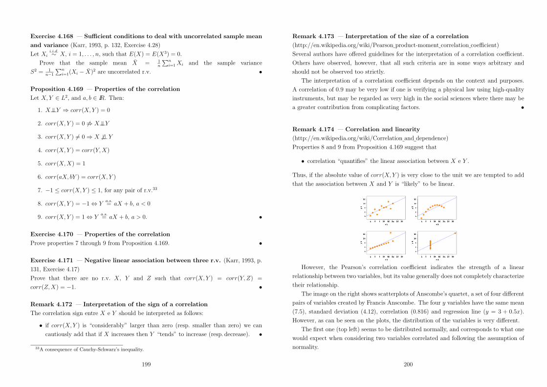
Exercise 4.168 — Su"cient conditions to deal with uncorrelated sample mean
and variance (Karr, 1993, p. 132, Exercise 4.28)
Let Xii.i.d./ X, i = 1, . . . , n, such that E(X) = E(X3) = 0.
Prove that the sample mean X = 1n
!ni=1 Xi and the sample variance
S2 = 1n$1
!ni=1(Xi ! X)2 are uncorrelated r.v. •
Proposition 4.169 — Properties of the correlation
Let X, Y " L2, and a, b " IR. Then:
1. X ::Y . corr(X, Y ) = 0
2. corr(X, Y ) = 0 &. X ::Y
3. corr(X, Y ) &= 0 . X :& :Y
4. corr(X, Y ) = corr(Y, X)
5. corr(X, X) = 1
6. corr(aX, bY ) = corr(X, Y )
7. !1 ' corr(X, Y ) ' 1, for any pair of r.v.33
8. corr(X, Y ) = !1 2 Ya.s.= aX + b, a < 0
9. corr(X, Y ) = 1 2 Ya.s.= aX + b, a > 0. •
Exercise 4.170 — Properties of the correlation
Prove properties 7 through 9 from Proposition 4.169. •
Exercise 4.171 — Negative linear association between three r.v. (Karr, 1993, p.
131, Exercise 4.17)
Prove that there are no r.v. X, Y and Z such that corr(X, Y ) = corr(Y, Z) =
corr(Z, X) = !1. •
Remark 4.172 — Interpretation of the sign of a correlation
The correlation sign entre X e Y should be interpreted as follows:
• if corr(X, Y ) is “considerably” larger than zero (resp. smaller than zero) we can
cautiously add that if X increases then Y “tends” to increase (resp. decrease). •
33A consequence of Cauchy-Schwarz’s inequality.
199
Remark 4.173 — Interpretation of the size of a correlation
(http://en.wikipedia.org/wiki/Pearson product-moment correlation coe$cient)
Several authors have o"ered guidelines for the interpretation of a correlation coe$cient.
Others have observed, however, that all such criteria are in some ways arbitrary and
should not be observed too strictly.
The interpretation of a correlation coe$cient depends on the context and purposes.
A correlation of 0.9 may be very low if one is verifying a physical law using high-quality
instruments, but may be regarded as very high in the social sciences where there may be
a greater contribution from complicating factors. •
Remark 4.174 — Correlation and linearity
(http://en.wikipedia.org/wiki/Correlation and dependence)
Properties 8 and 9 from Proposition 4.169 suggest that
• correlation “quantifies” the linear association between X e Y .
Thus, if the absolute value of corr(X, Y ) is very close to the unit we are tempted to add
that the association between X and Y is “likely” to be linear.
However, the Pearson’s correlation coe$cient indicates the strength of a linear
relationship between two variables, but its value generally does not completely characterize
their relationship.
The image on the right shows scatterplots of Anscombe’s quartet, a set of four di"erent
pairs of variables created by Francis Anscombe. The four y variables have the same mean
(7.5), standard deviation (4.12), correlation (0.816) and regression line (y = 3 + 0.5x).
However, as can be seen on the plots, the distribution of the variables is very di"erent.
The first one (top left) seems to be distributed normally, and corresponds to what one
would expect when considering two variables correlated and following the assumption of
normality.
200
The second one (top right) is not distributed normally; while an obvious relationship
between the two variables can be observed, it is not linear, and the Pearson correlation
coe$cient is not relevant.
In the third case (bottom left), the linear relationship is perfect, except for one outlier
which exerts enough influence to lower the correlation coe$cient from 1 to 0.816.
Finally, the fourth example (bottom right) shows another example when one outlier
is enough to produce a high correlation coe$cient, even though the relationship between
the two variables is not linear. •
Remark 4.175 — Correlation and causality
(http://en.wikipedia.org/wiki/Correlation and dependence)
The conventional dictum that “correlation does not imply causation” means that
correlation cannot be used to infer a causal relationship between the variables.34
This dictum should not be taken to mean that correlations cannot indicate the
potential existence of causal relations. However, the causes underlying the correlation,
if any, may be indirect and unknown, and high correlations also overlap with identity
relations, where no causal process exists. Consequently, establishing a correlation between
two variables is not a su$cient condition to establish a causal relationship (in either
direction).
Several sets of (x, y) points, with the correlation coe$cient of x and y for each set.
Note that the correlation reflects the noisiness and direction of a linear relationship (top
row), but not the slope of that relationship (middle), nor many aspects of nonlinear
relationships (bottom). The figure in the center has a slope of 0 but in that case the
correlation coe$cient is undefined because the variance of y is zero. •
34A correlation between age and height in children is fairly causally transparent, but a correlationbetween mood and health in people is less so. Does improved mood lead to improved health; or doesgood health lead to good mood; or both? Or does some other factor underlie both? In other words,a correlation can be taken as evidence for a possible causal relationship, but cannot indicate what thecausal relationship, if any, might be.
201
4.6.6 Moments of random vectors
Moments of random vectors are defined component, pairwise, etc. Instead of an expected
value (resp. variance) we shall deal with a mean vector (resp. covariance matrix).
Definition 4.176 — Mean vector and covariance matrix of a random vector
(Karr, 1993, p. 126)
Let X = (X1, . . . , Xd) be a d!dimensional random vector. Then provided that:
• Xi " L1, i = 1, . . . , d, the mean vector of X is the d!vector of the individual means,
µ = (E(X1), . . . , E(Xd));
• Xi " L2, i = 1, . . . , d, the covariance matrix of X is a d ) d matrix given by
'' = [cov(Xi, Xj)]i,j=1,...,d. •
Proposition 4.177 — Properties of the covariance matrix of a random vector
(Karr, 1993, p. 126)
Let X = (X1, . . . , Xd) be a d!dimensional random vector with covariance matrix ''.
Then:
• the diagonal of '' has entries equal to cov(Xi, Xi) = V (Xi), i = 1, . . . , d;
• '' is a symmetric matrix since cov(Xi, Xj) = cov(Xj, Xi), i, j = 1, . . . , d;
• '' is a positive-definite matrix, that is,!d
i=1
!dj=1 ci ) cov(Xi, Xj) ) cj > 0, for
every d!vector c = (c1, . . . , cd). •
Exercise 4.178 — Mean vector and covariance matrix of a linear combination
of r.v. (matrix notation)
Let:
• X = (X1, . . . , Xd) a d!dimensional random vector;
• µ = (E(X1), . . . , E(Xd)) the mean vector of X;
• '' = [cov(Xi, Xj)]i,j=1,...,d the covariance matrix of X;
• c = (c1, . . . , cd) a vector of weights.
By noting that!d
i=1 ci Xi = c2X, verify that:
• E9!d
i=1 ci Xi
:= c2 µ;
• V9!d
i=1 ci Xi
:= c2 '' c. •
202

4.6.7 Multivariate normal distributions
Motivation 4.179 — Multivariate normal distribution (Tong, 1990, p. 1)
There are many reasons for the predominance of the multivariate normal distribution:
• it represents a natural extension of the univariate normal distribution and provides
a suitable model for many real-life problems concerning vector-valued data;
• even if the original data cannot be fitted satisfactorily with a multivariate normal
distribution, by the central limit theorem the distribution of the sample mean vector
is asymptotically normal;
• the p.d.f. of a multivariate normal distribution is uniquely determined by the mean
vector and the covariance matrix;
• zero correlation imply independence between two components of the random vector
with multivariate normal distribution;
• the family of multivariate normal distributions is closed under linear transformations
or linear combinations;
• the marginal distribution of any subset of components of a random vector with
multivariate normal distribution is also multivariate normal;
• the conditional distribution in a multivariate normal distribution is also multivariate
normal. •
Remark 4.180 — Multivariate normal distribution (Tong, 1990, p. 2)
Studies of the bivariate normal distribution seem to begin in the middle of the XIX
century, and moved forward in 1888 with F. Galton’s (1822–1911) work on the applications
of correlations analysis in genetics. In 1896, K. Pearson (1857–1936) gave a definitive
mathematical formulation of the bivariate normal distribution.
The multivariate normal distribution was treated comprehensively for the first time
in 1892 by F.Y. Edgeworth (1845–1926). •
A random vector has a multivariate normal distribution if it is a linear transformation
of a random vector with i.i.d. components with standard normal distribution (Karr, 1993,
p. 126).
203
Definition 4.181 — Multivariate normal distribution (Karr, 1993, p. 126)
Let:
• µ = (µ1, . . . , µd) " IRd;
• '' = [#ij]i,j=1,...,d be a symmetric, positive-definite, non-singular d) d matrix;35
Then the random vector X = (X1, . . . , Xd) has a multivariate normal distribution with
mean vector µ and covariance matrix '' if
X = ''12 Y + µ, (4.118)
where:
• Y = (Y1, . . . , Yd) with Yii.i.d./ Normal(0, 1), i = 1, . . . , d;
• ''12 is the unique matrix satisfying
9''
12
:2) ''
12 = ''.
In this case we write X / Normald(µ, ''). •
We can use Definition 4.181 to simulate a multivariate normal distribution as
mentioned below.
Remark 4.182 — Simulating a multivariate normal distribution (Gentle, 1998,
pp. 105–106)
Since Yii.i.d./ Normal(0, 1), i = 1, . . . , d, implies that X = ''
12 Y + µ / Normald(µ, '')
we can obtain a d!dimensional pseudo-random vector from this multivariate normal
distribution if we:
1. generate d independent pseudo-random numbers, y1, . . . , yd, from the standard
normal distribution;
2. assign x = ''12 y + µ, where y = (y1, . . . , yd).
Gentle (1998, p. 106) refers other procedures to generate pseudo-random numbers with
multivariate normal distribution. •
35A d ) d matrix A is called invertible or non-singular or non-degenerate if there exists and ) d matrix B such that AB = BA = Id, where Id denotes the d ) d identity matrix.(http://en.wikipedia.org/wiki/Invertible matrix) .
204
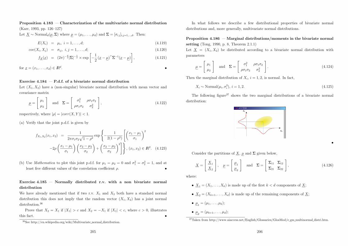
Proposition 4.183 — Characterization of the multivariate normal distribution
(Karr, 1993, pp. 126–127)
Let X / Normald(µ, '') where µ = (µ1, . . . , µd) and '' = [#i j]i,j=1,...,d. Then:
E(Xi) = µi, i = 1, . . . , d; (4.119)
cov(Xi, Xj) = #ij, i, j = 1, . . . , d; (4.120)
fX(x) = (2")$d2 |''|$ 1
2 ) exp
I!1
2(x! µ)2''$1(x! µ)
J, (4.121)
for x = (x1, . . . , xd) " IRd. •
Exercise 4.184 — P.d.f. of a bivariate normal distribution
Let (X1, X2) have a (non-singular) bivariate normal distribution with mean vector and
covariance matrix
µ =
Bµ1
µ2
Cand '' =
B#2
1 (#1#2
(#1#2 #22
C, (4.122)
respectively, where |(| = |corr(X, Y )| < 1.
(a) Verify that the joint p.d.f. is given by
fX1,X2(x1, x2) =1
2"#1#2
K1! (2
exp
7! 1
2(1! (2)
B'x1 ! µ1
#1
(2
!2(
'x1 ! µ1
#1
( 'x2 ! µ2
#2
(+
'x2 ! µ2
#2
(2C=
, (x1, x2) " IR2. (4.123)
(b) Use Mathematica to plot this joint p.d.f. for µ1 = µ2 = 0 and #21 = #2
2 = 1, and at
least five di"erent values of the correlation coe$cient (. •
Exercise 4.185 — Normally distributed r.v. with a non bivariate normal
distribution
We have already mentioned that if two r.v. X1 and X2 both have a standard normal
distribution this does not imply that the random vector (X1, X2) has a joint normal
distribution.36
Prove that X2 = X1 if |X1| > c and X2 = !X1 if |X1| < c, where c > 0, illustrates
this fact. •36See http://en.wikipedia.org/wiki/Multivariate normal distribution.
205
In what follows we describe a few distributional properties of bivariate normal
distributions and, more generally, multivariate normal distributions.
Proposition 4.186 — Marginal distributions/moments in the bivariate normal
setting (Tong, 1990, p. 8, Theorem 2.1.1)
Let X = (X1, X2) be distributed according to a bivariate normal distribution with
parameters
µ =
Bµ1
µ2
Cand '' =
B#2
1 (#1#2
(#1#2 #22
C. (4.124)
Then the marginal distribution of Xi, i = 1, 2, is normal. In fact,
Xi / Normal(µi, #2i ), i = 1, 2. (4.125)
The following figure37 shows the two marginal distributions of a bivariate normal
distribution:
•
Consider the partitions of X, µ and '' given below,
X =
BX1
X2
C, µ =
Bµ
1
µ2
Cand '' =
B''11 ''12
''21 ''22
C, (4.126)
where:
• X1 = (X1, . . . , Xk) is made up of the first k < d components of X;
• X2 = (Xk+1, . . . , Xd) is made up of the remaining components of X;
• µ1
= (µ1, . . . , µk);
• µ2
= (µk+1, . . . , µd);
37Taken from http://www.aiaccess.net/English/Glossaries/GlosMod/e gm multinormal distri.htm.
206

• ''11 = [#ij]i,j=1,...,k; ''12 = [#ij]1'i<j'k;
• ''21 = ''212;
• ''22 = [#ij]i,j=k+1,...,d.
The following figure (where d = p)38 represents the covariance matrix of X1, ''11, which
is just the upper left corner square submatrix of order k of the original covariance matrix:
Theorem 4.187 — Marginal distributions/moments in the multivariate normal
setting (Tong, 1990, p. 30, Theorem 3.3.1)
Let X / Normald(µ, ''). Then for every k < d the marginal distributions of X1 and X2
are also multivariate normal:
X1 / Normalk(µ1, ''11) (4.127)
X2 / Normald$k(µ2, ''22), (4.128)
respectively. •
The family of multivariate normal distributions is closed under linear transformations,
as stated below.
Theorem 4.188 — Distribution/moments of a linear transformation of a
bivariate normal random vector (Tong, 1990, p. 10, Theorem 2.1.2)
Let:
• X / Normal2(µ, '');
• C = [cij] be a 2) 2 real matrix;
• b = (b1, b2) be a real vector.
Then
Y = CX + b / Normal2(Cµ + b,C''C2). (4.129)
•38Also taken from http://www.aiaccess.net/English/Glossaries/GlosMod/e gm multinormal distri.htm.
207
Exercise 4.189 — Distribution/moments of a linear transformation of a
bivariate normal random vector
(a) Prove that if in Theorem 4.188 we choose
C =
B#$1
1 0
0 #$12
C(4.130)
and b = !Cµ, then Y is a bivariate normal variable with zero means, unit variances
and correlation coe$cient ( (Tong, 1990, p. 10).
(b) Now consider a linear transformation of Y , Y ,, by rotating the xy axes by 45 degrees
counterclockwise:
Y , =1+2
B1 !1
1 1
CY . (4.131)
Verify that Y , is a bivariate normal variable with zero means, variances 1 ! ( and
1 + ( and null correlation coe$cient (Tong, 1990, p. 10). Comment.
(c) Conclude that if X / Normal2(µ, '') such that |(| < 1 then
B1%1$$
0
0 1%1+$
C B1%2! 1%
21%2
1%2
C B#$1
1 0
0 #$12
C BX1 ! µ1
X2 ! µ2
C/ Normal2(0, I2), (4.132)
where 0 = (0, 0) and I2 is the 2) 2 identity matrix (Tong, 1990, p. 11).
(d) Prove that if Zii.i.d./ Normal(0, 1) then
B#1 0
0 #2
C B1%2
1%2
! 1%2
1%2
C B +1! ( 0
0+
1 + (
C BZ1
Z2
C+
Bµ1
µ2
C
st=
B#1 0
#2( #2
K1! (2
C BZ1
Z2
C+
Bµ1
µ2
C/ Normal2(µ, ''),
(4.133)
i.e. we can obtain a bivariate normal distribution with any mean vector
and (non-singular, semi-definite positive) covariance matrix through a
transformation of two independent standard normal r.v. (Tong, 1990, p. 11;
http://xbeta.org/wiki/show/Bivariate+normal+distribution). •
208

Theorem 4.190 — Distribution/moments of a linear transformation of a
multivariate normal distribution (Tong, 1990, p. 32, Theorem 3.3.3)
Let:
• X / Normald(µ, '');
• C = [cij] be any given k ) d real matrix;
• b is any k ) 1 real vector.
Then
Y = CX + b / Normalk(Cµ + b,C''C2). (4.134)
•
The family of multivariate normal distributions is closed not only under linear
transformations, as stated in the previous theorem, but also under linear combinations.
Corollary 4.191 — Distribution/moments of a linear combination of the
components of a multivariate normal random vector (Tong, 1990, p. 33, Corollary
3.3.3)
Let:
• X / Normald(µ, '') partitioned as in (4.126);
• C1 and C2 be two m) k and m) (d! k) real matrices, respectively.
Then
Y = C1 X1 + C2 X2 / Normalm(µY, ''Y ), (4.135)
where the mean vector and the covariance matrix of Y are given by
µY
= C1 µ1+ C2 µ
2(4.136)
''Y = C1 ''11 C21 + C2 ''22 C2
2 + C1 ''12 C22 + C2 ''21 C2
1 , (4.137)
respectively. •
209
The result that follows has already been proved in Chapter 3 and is a particular case
of Theorem 4.193.
Corollary 4.192 — Correlation and independence in a bivariate normal setting
(Tong, 1990, p. 8, Theorem 2.1.1)
Let X = (X1, X2) / Normal2(µ, ''). Then X1 and X2 are independent i" ( = 0. •
In general, r.v. may be uncorrelated but highly dependent. But if a random vector
has a multivariate normal distribution then any two or more of its components that are
uncorrelated are independent.
Theorem 4.193 — Correlation and independence in a multivariate normal
setting (Tong, 1990, p. 31, Theorem 3.3.2)
Let X / Normald(µ, '') partitioned as in (4.126). Then X1 and X2 are independent
random vectors i" ''12 = ''212 = 0k/(d$k). •
Corollary 4.194 — Linear combination of independent multivariate normal
random vectors (Tong, 1990, p. 33, Corollary 3.3.4)
Let X1, . . . , XN be independent Normald(µi, ''i), i = 1, . . . , N , random vectors. Then
Y =N%
i=1
ci X i / Normald
"N%
i=1
ci µi,
N%
i=1
c2i ''i
$. (4.138)
•
Proposition 4.195 — Independence between the sample mean vector and
covariance matrix (Tong, 1990, pp. 47–48)
Let:
• N be a positive integer;
• X1, . . . , XN be i.i.d. random vectors with a common Normald(µ, '') distribution,
such that '' is positive definite;
• XN = 1N
!Nt=1 X t = (X1, . . . , Xd) denote the sample mean vector, where
Xi = 1N
!Nt=1 Xit and Xit the ith component of X t;
• SN = [Sij]i,j=1,...,d denote the sample covariance matrix, where
Sij = 1N$1
!Nt=1(Xit ! Xi)(Xjt ! Xj).
Then XN and SN are independent. •
210
Definition 4.196 — Mixed (central) moments
Let:
• X = (X1, . . . , Xd) be a random d!vector;
• r1, . . . , rd " IN .
Then:
• the mixed moment of order (r1, . . . , rd) of X is given by
E [Xr11 ) . . .)Xrd
d ] , (4.139)
and is also called a (!d
i=1 ri)th order moment of X;39
• the mixed central moment of order (r1, . . . , rd) of X is defined as
E {[X1 ! E(X1)]r1 ) . . . [Xd ! E(Xd)]
rd} . (4.140)
•
The Isserlis’ theorem is a formula that allows one to compute mixed moments of the
multivariate normal distribution with null mean vector40 in terms of the entries of its
covariance matrix.
Remarks 4.197 — Isserlis’ theorem (http://en.wikipedia.org/wiki/Isserlis’ theorem)
• In his original paper from 1918, Isserlis considered only the fourth-order moments,
in which case the formula takes appearance
E(X1X2X3X4) = E(X1X2)) E(X3X4) + E(X1X3)) E(X2X4)
+E(X1X4)) E(X2X3), (4.141)
which can be written in terms of the covariances: #12 ) #34 + #13 ) #24 + #14 ) #23.
It also added that if (X1, . . . , X2n) is a zero mean multivariate normal random vector,
then
E(X1 . . . X2n$1) = 0 (4.142)
E(X1 . . . X2n) =% &
E(XiXj), (4.143)
39See for instance http://en.wikipedia.org/wiki/Multivariate normal distribution.40Or mixed moments of the di"erence between a multivariate normal random vector X and its mean
vector.
211
where the notation! A
means summing over all distinct ways of partitioning
X1, . . . , X2n into pairs.
• This theorem is particularly important in particle physics, where it is known as
Wick’s theorem.
• Another applications include the analysis of portfolio returns, quantum field theory,
generation of colored noise, etc. •
Theorem 4.198 — Isserlis’ theorem
(http://en.wikipedia.org/wiki/Multivariate normal distribution)
Let:
• X = (X1, . . . , Xd) / Normald(µ, '');
• EGAd
i=1(Xi ! µi)ri
Hbe the mixed central moment of order (r1, . . . , rd) of X;
• k =!d
i=1 ri.
Then:
• if k is odd (i.e. k = 2n! 1, n " IN)
E
Bd&
i=1
(Xi ! µi)ri
C= 0; (4.144)
• if k is even (i.e. k = 2n, n " IN)
E
Bd&
i=1
(Xi ! µi)ri
C=
% &#ij, (4.145)
where the! A
is taken over all allocations of the set {1, 2, . . . , n} into n (unordered)
pairs, that is, if you have a k = 2n = 6th order central moment, you will be summing
the products of n = 3 covariances. •
212
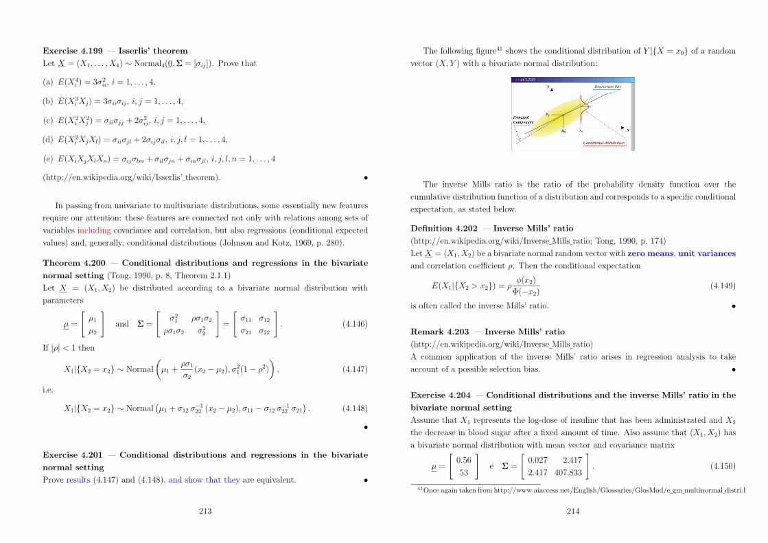
Exercise 4.199 — Isserlis’ theorem
Let X = (X1, . . . , X4) / Normal4(0, '' = [#ij]). Prove that
(a) E(X4i ) = 3#2
ii, i = 1, . . . , 4,
(b) E(X3i Xj) = 3#ii#ij, i, j = 1, . . . , 4,
(c) E(X2i X2
j ) = #ii#jj + 2#2ij, i, j = 1, . . . , 4,
(d) E(X2i XjXl) = #ii#jl + 2#ij#il, i, j, l = 1, . . . , 4,
(e) E(XiXjXlXn) = #ij#lm + #il#jn + #in#jl, i, j, l, n = 1, . . . , 4
(http://en.wikipedia.org/wiki/Isserlis’ theorem). •
In passing from univariate to multivariate distributions, some essentially new features
require our attention: these features are connected not only with relations among sets of
variables including covariance and correlation, but also regressions (conditional expected
values) and, generally, conditional distributions (Johnson and Kotz, 1969, p. 280).
Theorem 4.200 — Conditional distributions and regressions in the bivariate
normal setting (Tong, 1990, p. 8, Theorem 2.1.1)
Let X = (X1, X2) be distributed according to a bivariate normal distribution with
parameters
µ =
Bµ1
µ2
Cand '' =
B#2
1 (#1#2
(#1#2 #22
C=
B#11 #12
#21 #22
C. (4.146)
If |(| < 1 then
X1|{X2 = x2} / Normal
'µ1 +
(#1
#2(x2 ! µ2), #
21(1! (2)
(, (4.147)
i.e.
X1|{X2 = x2} / Normal-µ1 + #12 #$1
22 (x2 ! µ2), #11 ! #12 #$122 #21
.. (4.148)
•
Exercise 4.201 — Conditional distributions and regressions in the bivariate
normal setting
Prove results (4.147) and (4.148), and show that they are equivalent. •
213
The following figure41 shows the conditional distribution of Y |{X = x0} of a random
vector (X, Y ) with a bivariate normal distribution:
The inverse Mills ratio is the ratio of the probability density function over the
cumulative distribution function of a distribution and corresponds to a specific conditional
expectation, as stated below.
Definition 4.202 — Inverse Mills’ ratio
(http://en.wikipedia.org/wiki/Inverse Mills ratio; Tong, 1990, p. 174)
Let X = (X1, X2) be a bivariate normal random vector with zero means, unit variances
and correlation coe$cient (. Then the conditional expectation
E(X1|{X2 > x2}) = (.(x2)
#(!x2)(4.149)
is often called the inverse Mills’ ratio. •
Remark 4.203 — Inverse Mills’ ratio
(http://en.wikipedia.org/wiki/Inverse Mills ratio)
A common application of the inverse Mills’ ratio arises in regression analysis to take
account of a possible selection bias. •
Exercise 4.204 — Conditional distributions and the inverse Mills’ ratio in the
bivariate normal setting
Assume that X1 represents the log-dose of insuline that has been administrated and X2
the decrease in blood sugar after a fixed amount of time. Also assume that (X1, X2) has
a bivariate normal distribution with mean vector and covariance matrix
µ =
B0.56
53
Ce '' =
B0.027 2.417
2.417 407.833
C. (4.150)
41Once again taken from http://www.aiaccess.net/English/Glossaries/GlosMod/e gm multinormal distri.htm.
214

(a) Obtain the probability that the decrease in blood sugar exceeds 70, given that log-dose
of insuline that has been administrated is equal to 0.5.
(b) Determine the log-dose of insuline that has to be administrated so that the expected
value of the decrease in blood sugar equals 70.
(c) Obtain the expected value of the decrease in blood sugar, given that log-dose of
insuline that has been administrated exceeds 0.5. •
Theorem 4.205 — Conditional distributions and regressions in the
multivariate normal setting (Tong, 1990, p. 35, Theorem 3.3.4)
Let X / Normald(µ, '') partitioned as in (4.126). Then
X1|{X2 = x2} / Normalk9µ
1+ ''12 ''$1
22 (x2 ! µ2), ''11 ! ''12 ''$1
22 ''21
:. (4.151)
•
Exercise 4.206 — Conditional distributions and regressions in the multivariate
normal setting
Derive (4.148) from (4.151). •
215
4.6.8 Multinomial distributions
The genesis and the definition of multinomial distributions follow.
Motivation 4.207 — Multinomial distribution
(http://en.wikipedia.org/wiki/Multinomial distribution)
The multinomial distribution is a generalization of the binomial distribution.
The binomial distribution is the probability distribution of the number of “successes”
in n independent Bernoulli trials, with the same probability of “success” on each trial.
In a multinomial distribution, the analog of the Bernoulli distribution is the categorical
distribution, where each trial results in exactly one of some fixed finite number d of possible
outcomes, with probabilities p1, . . . , pd (pi " [0, 1], i = 1, . . . , d, and!d
i=1 pi = 1), and
there are n independent trials. •
Definition 4.208 — Multinomial distribution (Johnson and Kotz, 1969, p. 281)
Consider a series of n independent trials, in each of which just one of d mutually exclusive
events E1, . . . , Ed must be observed, and in which the probability of occurrence of event
Ei is equal to pi for each trial, with, of course, pi " [0, 1], i = 1, . . . , d, and!d
i=1 pi = 1.
Then the joint distribution of the r.v. N1, . . . , Nd, representing the numbers of occurrences
of the events E1, . . . , Ed (respectively) in n trials, is defined by
P ({N1 = n1, . . . , Nd = nd}) =n!
Adi=1 ni!
)d&
i=1
pnii , (4.152)
for ni " IN0, i = 1, . . . , d, such that!d
i=1 ni = n. The random d!vector N = (N1, . . . , Nd)
is said to have a multinomial distribution with parameters n and p = (p1, . . . , pd)) — in
short N / Multinomiald$1(n, p = (p1, . . . , pd)).42 •
Remark 4.209 — Special case of the multinomial distribution (Johnson and Kotz,
1969, p. 281)
Needless to say, we deal with the binomial distribution when d = 2, i.e.,
Multinomial2$1(n, p = (p, 1! p))d= Binomial(n, p). (4.153)
Curiously, J. Bernoulli, who worked with the binomial distribution, also used the
multinomial distribution. •42The index d! 1 follows from the fact that the r.v. Nd (or any other component of N) is redundant:
Nd = n!!d!1
i=1 Ni.
216
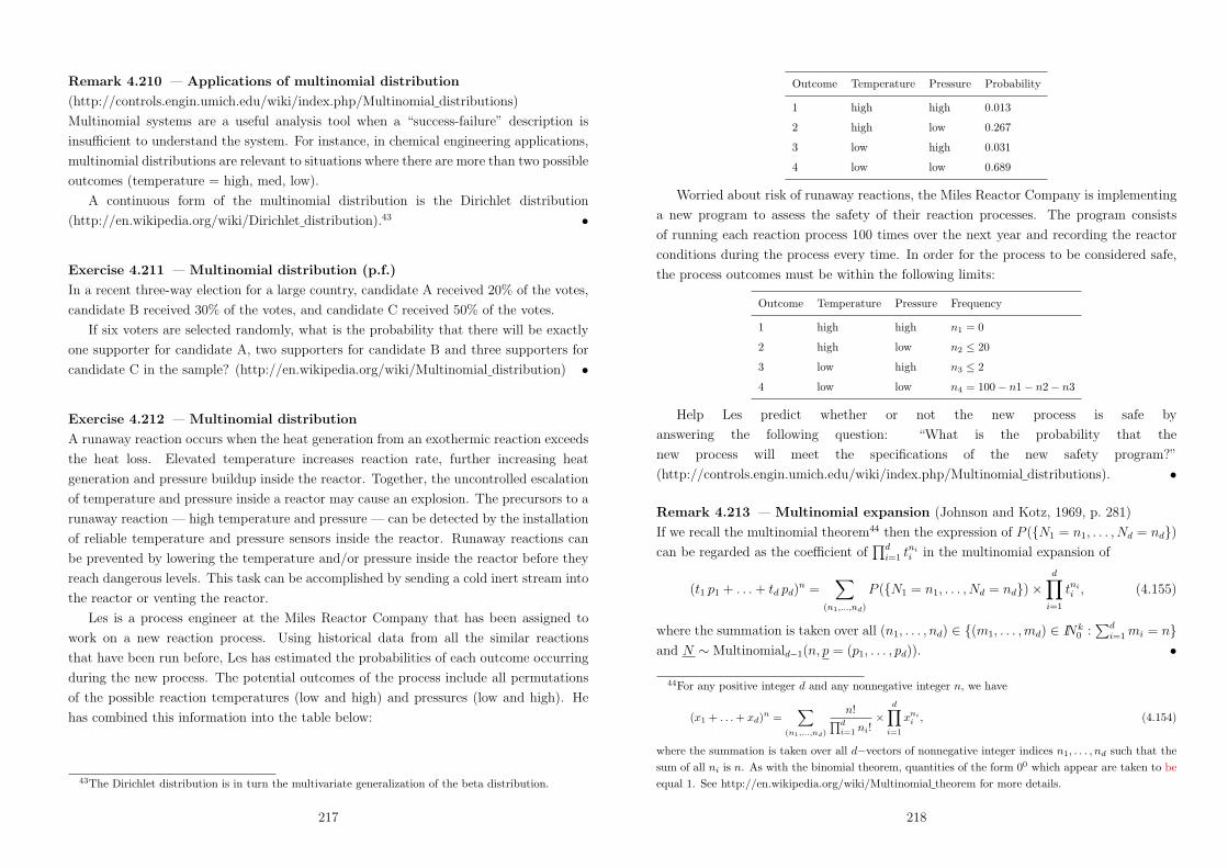
Remark 4.210 — Applications of multinomial distribution
(http://controls.engin.umich.edu/wiki/index.php/Multinomial distributions)
Multinomial systems are a useful analysis tool when a “success-failure” description is
insu$cient to understand the system. For instance, in chemical engineering applications,
multinomial distributions are relevant to situations where there are more than two possible
outcomes (temperature = high, med, low).
A continuous form of the multinomial distribution is the Dirichlet distribution
(http://en.wikipedia.org/wiki/Dirichlet distribution).43 •
Exercise 4.211 — Multinomial distribution (p.f.)
In a recent three-way election for a large country, candidate A received 20% of the votes,
candidate B received 30% of the votes, and candidate C received 50% of the votes.
If six voters are selected randomly, what is the probability that there will be exactly
one supporter for candidate A, two supporters for candidate B and three supporters for
candidate C in the sample? (http://en.wikipedia.org/wiki/Multinomial distribution) •
Exercise 4.212 — Multinomial distribution
A runaway reaction occurs when the heat generation from an exothermic reaction exceeds
the heat loss. Elevated temperature increases reaction rate, further increasing heat
generation and pressure buildup inside the reactor. Together, the uncontrolled escalation
of temperature and pressure inside a reactor may cause an explosion. The precursors to a
runaway reaction — high temperature and pressure — can be detected by the installation
of reliable temperature and pressure sensors inside the reactor. Runaway reactions can
be prevented by lowering the temperature and/or pressure inside the reactor before they
reach dangerous levels. This task can be accomplished by sending a cold inert stream into
the reactor or venting the reactor.
Les is a process engineer at the Miles Reactor Company that has been assigned to
work on a new reaction process. Using historical data from all the similar reactions
that have been run before, Les has estimated the probabilities of each outcome occurring
during the new process. The potential outcomes of the process include all permutations
of the possible reaction temperatures (low and high) and pressures (low and high). He
has combined this information into the table below:
43The Dirichlet distribution is in turn the multivariate generalization of the beta distribution.
217
Outcome Temperature Pressure Probability
1 high high 0.013
2 high low 0.267
3 low high 0.031
4 low low 0.689
Worried about risk of runaway reactions, the Miles Reactor Company is implementing
a new program to assess the safety of their reaction processes. The program consists
of running each reaction process 100 times over the next year and recording the reactor
conditions during the process every time. In order for the process to be considered safe,
the process outcomes must be within the following limits:
Outcome Temperature Pressure Frequency
1 high high n1 = 0
2 high low n2 ' 20
3 low high n3 ' 2
4 low low n4 = 100! n1! n2! n3
Help Les predict whether or not the new process is safe by
answering the following question: “What is the probability that the
new process will meet the specifications of the new safety program?”
(http://controls.engin.umich.edu/wiki/index.php/Multinomial distributions). •
Remark 4.213 — Multinomial expansion (Johnson and Kotz, 1969, p. 281)
If we recall the multinomial theorem44 then the expression of P ({N1 = n1, . . . , Nd = nd})can be regarded as the coe$cient of
Adi=1 tni
i in the multinomial expansion of
(t1 p1 + . . . + td pd)n =
%
(n1,...,nd)
P ({N1 = n1, . . . , Nd = nd}))d&
i=1
tnii , (4.155)
where the summation is taken over all (n1, . . . , nd) " {(m1, . . . ,md) " INk0 :
!di=1 mi = n}
and N / Multinomiald$1(n, p = (p1, . . . , pd)). •
44For any positive integer d and any nonnegative integer n, we have
(x1 + . . . + xd)n =%
(n1,...,nd)
n!Ad
i=1 ni!)
d&
i=1
xnii , (4.154)
where the summation is taken over all d!vectors of nonnegative integer indices n1, . . . , nd such that thesum of all ni is n. As with the binomial theorem, quantities of the form 00 which appear are taken to beequal 1. See http://en.wikipedia.org/wiki/Multinomial theorem for more details.
218
Definition 4.214 — Mixed factorial moments
Let:
• X = (X1, . . . , Xd) be a random d!vector;
• r1, . . . , rd " IN0.
Then the mixed factorial moment of order (r1, . . . , rd) of X is equal to
EGX(r1)
1 ) . . .)X(rd)d
H
= E {[X1(X1 ! 1) . . . (X1 ! r1 + 1)]) . . .) [Xd(Xd ! 1) . . . (Xd ! rd + 1)]} . (4.156)
•
Marginal moments and marginal central moments, and covariances and correlations
between the components of a random vector can be written in terms of mixed
(central/factorial) moments. This is particularly useful when we are dealing with the
multinomial distribution.
Exercise 4.215 — Writing the variance and covariance in terms of mixed
(central/factorial) moments
Write
(a) the marginal variance of Xi and
(b) cov(Xi, Xj)
in terms of mixed factorial moments. •
Proposition 4.216 — Mixed factorial moments of a multinomial distribution
(Johnson and Kotz, 1969, p. 284)
Let:
• N = (N1, . . . , Nd) / Multinomiald$1(n, p = (p1, . . . , pd));
• r1, . . . , rd " IN0.
Then the mixed factorial moment of order (r1, . . . , rd) is equal to
EGN (r1)
1 ) . . .)N (rd)d
H= n(
Pdi=1 ri) )
d&
i=1
prii , (4.157)
where n(Pd
i=1 ri) = n!(n$
Pdi=1 ri))!
. •
219
From the general formula (4.157), we find the expected value of Ni, and the covariances
and correlations between Ni and Nj.
Corollary 4.217 — Mean vector, covariance and correlation matrix
of a multinomial distribution (Johnson and Kotz, 1969, p. 284;
http://en.wikipedia.org/wiki/Multinomial distribution)
The expected number of times the event Ei was observed over n trials, Ni, is
E(Ni) = n pi, (4.158)
for i = 1, . . . , d.
The covariance matrix is as follows. Each diagonal entry is the variance
V (Ni) = n pi (1! pi), (4.159)
for i = 1, . . . , d. The o"-diagonal entries are the covariances
cov(Ni, Nj) = !n pi pj, (4.160)
for i, j = 1, . . . , d, i &= j. All covariances are negative because, for fixed n, an increase in
one component of a multinomial vector requires a decrease in another component. The
covariance matrix is a d) d positive-semidefinite matrix of rank d! 1.
The o"-diagonal entries of the corresponding correlation matrix are given by
corr(Ni, Nj) = !N
pi pj
(1! pi) (1! pj), (4.161)
for i, j = 1, . . . , d, i &= j.45 Note that the number of trials (n) drops out of the expression
of corr(Ni, Nj). •
Exercise 4.218 — Mean vector, covariance and correlation matrices of a
multinomial distribution
Use (4.157) to derive the entries of the mean vector, and the covariance and correlation
matrices of a multinomial distribution. •
Exercise 4.219 — Mean vector and correlation matrix of a multinomial
distribution
Resume Exercise 4.211 and calculate the mean vector and the correlation matrix.
Comment the values you have obtained for the o"-diagonal entries of the correlation
matrix. •45The diagonal entries of the correlation matrix are obviously equal to 1.
220

Proposition 4.220 — Marginal distributions in a multinomial setting (Johnson
and Kotz, 1969, p. 281)
The marginal distribution of any Ni, i = 1, . . . , d, is Binomial with parameters n and pi.
I.e.
Ni / Binomial(n, pi). (4.162)
for i = 1, . . . , d. •
(4.162) is a special case of a more general result.
Proposition 4.221 — Joint distribution of a subset of r.v. from a multinomial
distribution (Johnson and Kotz, 1969, p. 281)
The joint distribution of any subset of s (s = 1, . . . , d ! 1) r.v., say Na1 , . . . , Nas of the
Nj’s, is also multinomial with an (s + 1)th r.v. equal to Nas+1 = n!!s
i=1 Nai . In fact
P-E
Na1 = na1 , . . . , Nas = nas , Nas+1 = n!!s
i=1 nai
F.
= n!Qsi=1 nai !/(n$
Psi=1 nai )!
)As
i=1
Ip
naiai )
91!
!sj=1 paj
:n$Ps
j=1 naj
J,
(4.163)
for nai " IN0, i = 1, . . . , s such that!s
i=1 nai ' n. •
Proposition 4.222 — Some regressions and conditional distributions in the
multinomial distribution setting (Johnson and Kotz, 1969, p. 284)
• The regression of Ni on Nj (j &= i) is linear:
E(Ni|Nj) = (n!Nj))pi
1! pj. (4.164)
• The multiple regression of Ni on Nb1 , . . . , Nbr (bj &= i, j = 1, . . . , r) is also linear:
E(Ni|{Nb1 , . . . , Nbr}) =
"n!
r%
j=1
Nbj
$) pi
1!!r
j=1 pbj
. (4.165)
• The random vector (Na1 , . . . Nas) conditional on a event referring to any subset of the
remaining Nj’s, say {Nb1 = nb1 , . . . , Nbr = nbr}, has also a multinomial distribution.
Its p.f. can be found in Johnson and Kotz (1969, p. 284). •
221
Remark 4.223 — Conditional distributions and the simulation of a
multinomial distribution (Gentle, 1998, p. 106)
The following conditional distributions taken from Gentle (1998, p. 106) suggest a
procedure to generate pseudo-random vectors with a multinomial distribution:
• N1 / Binomial(n, p1);
• N2|{N1 = n1} / Binomial9n! n1,
p2
1$p1
:;
• N3|{N1 = n1, N2 = n2} / Binomial9n! n1 ! n2,
p3
1$p1$p2
:;
• . . .
• Nd$1|{N1 = n1, . . . , Nd$2 = nd$2} / Binomial9n!
!d$2i=1 ni,
pd!1
1$Pd!2
i=1 pi
:;
• Nd|{N1 = n1, . . . , Nd$1 = nd$1}d= n!
!d$1i=1 ni.
Thus, we can generate a pseudo-random vector from a multinomial distribution
by sequentially generating independent pseudo-random numbers from the binomial
conditional distributions stated above.
Gentle (1998, p. 106) refers other ways of generating pseudo-random vectors from a
multinomial distribution. •
Remark 4.224 — Speeding up the simulation of a multinomial distribution
(Gentle, 1998, p. 106)
To speed up the generation process, Gentle (1998, p. 106) recommends that we previously
order the probabilities p1, . . . , pd in descending order — thus, getting the vector of
probabilities (p(d), . . . , p(1)), where p(d) = maxi=1,...,d pi, . . ., and p(1) = mini=1,...,d pi. Then
we generate d pseudo-random numbers with the following binomial distributions with
parameters
1. n and the largest probability of “success” p(d), say n(d),
2. n! n(d) andp(d!1)
1$p(d!1), say n(d$1),
3. n! n(d) ! n(d$1) andp(d!2)
1$p(d!1)$p(d!2), say n(d$1),
4. . . .
5. n!!d$2
i=1 n(d+1$i) andp(2)
1$Pd!2
i=1 p(d+1!i), say n(2),
222

and finally
6. assign n(1) = n!!d$1
i=1 n(d+1$i). •
Remark 4.225 — Speeding up the simulation of a multinomial distribution
(http://en.wikipedia.org/wiki/Multinomial distribution)
Assume the parameters p1, . . . pd are already sorted descendingly (this is only to speed up
computation and not strictly necessary). Now, for each trial, generate a pseudo-random
number from U / Uniform(0, 1), say u. The resulting outcome is the event Ej where
j = arg minj#=1,...,k
"j#%
i=1
pi - u
$
= F$1Z (u), (4.166)
with Z an integer r.v. that takes values 1, . . . , d, with probabilities p1, . . . pd, respectively.
This is a sample for the multinomial distribution with n = 1.
The absolute frequencies of events E1, . . . , Ed, resulting from n independent repetitions
of the procedure we just described, constitutes a pseudo-random vector from a multinomial
distribution with parameters n and p = (p1, . . . pd). •
References
• Gentle, J.E. (1998). Random Number Generation and Monte Carlo Methods.
Springer-Verlag. (QA298.GEN.50103)
• Johnson, N.L. and Kotz, S. (1969). Discrete distributions John Wiley & Sons.
(QA273-280/1.JOH.36178)
• Karr, A.F. (1993). Probability. Springer-Verlag.
• Resnick, S.I. (1999). A Probability Path. Birkhauser. (QA273.4-.67.RES.49925)
• Rohatgi, V.K. (1976). An Introduction to Probability Theory and Mathematical
Statistics. John Wiley & Sons. (QA273-280/4.ROH.34909)
• Tong, Y.L. (1990). The Multivariate Normal Distribution. Springer-Verlag.
(QA278.5-.65.TON.39685)
• Walrand, J. (2004). Lecture Notes on Probability Theory and Random Processes.
Department of Electrical Engineering and Computer Sciences, University of
California, Berkeley.
223
Chapter 5
Convergence concepts and classical
limit theorems
Throughout this chapter we assume that {X1, X2, . . .} is a sequence of r.v. and X is a
r.v., and all of them are defined on the same probability space (!,F , P ).
Stochastic convergence formalizes the idea that a sequence of r.v. sometimes is
expected to settle into a pattern.1 The pattern may for instance be that:
• there is a convergence of Xn(!) in the classical sense to a fixed value X(!), for each
and every event !;
• the probability that the distance between Xn from a particular r.v. X exceeds any
prescribed positive value decreases and converges to zero;
• the sequence formed by calculating the expected value of the (absolute or quadratic)
distance between Xn and X converges to zero;
• the distribution of Xn may “grow” increasingly similar to the distribution of a
particular r.v. X.
Just as in real analysis, we can distinguish among several types of convergence
(Rohatgi, 1976, p. 240). Thus, in this chapter we investigate modes of convergence of
sequences of r.v.:
• almost sure convergence (a.s.4);
• convergence in probability (P4);
1See http://en.wikipedia.org/wiki/Convergence of random variables.
224

• convergence in quadratic mean or in L2 (q.m.4 );
• convergence in L1 or in mean (L1
4);
• convergence in distribution (d4).
It is important for the reader to be familiarized with all these modes of convergence,
the way they can be related and with the applications of such results and understand
their considerable significance in probability, statistics and stochastic processes.
5.1 Modes of convergence
The first four modes of convergence (,4, where @ = a.s., P, q.m., L1) pertain to the
sequence of r.v. and to X as functions of !, while the fifth (d4) is related to the convergence
of d.f. (Karr, 1993, p. 135).
5.1.1 Convergence of r.v. as functions on !
Motivation 5.1 — Almost sure convergence (Karr, 1993, p. 135)
Almost sure convergence — or convergence with probability one — is the probabilistic
version of pointwise convergence known from elementary real analysis. •
Definition 5.2 — Almost sure convergence (Karr, 1993, p. 135; Rohatgi, 1976, p.
249)
The sequence of r.v. {X1, X2, . . .} is said to converge almost surely to a r.v. X if
P
'Lw : lim
n&+!Xn(!) = X(!)
M(= 1. (5.1)
In this case we write Xna.s.4 X (or Xn 4 X with probability 1). •
Remark 5.3 — Almost sure convergence
Equation (5.1) does not mean that limn&+! P ({w : Xn(!) = X(!)}) = 1. •
Exercise 5.4 — Almost sure convergence
Let {X1, X2, . . .} be a sequence of independent r.v. such that Xn / Bernoulli( 1n), n " IN .
Prove that Xn &a.s.4 0, by deriving P ({Xn = 0, for every m ' n ' n0}) and observing
that this probability does not converge to 1 as n0 4 +, for all values of m (Rohatgi,
1976, p. 252, Example 9). •
225
Motivation 5.5 — Convergence in probability (Karr, 1993, p. 135;
http://en.wikipedia.org/wiki/Convergence of random variables)
Convergence in probability essentially means that the probability that |Xn !X| exceeds
any prescribed, strictly positive value converges to zero.
The basic idea behind this type of convergence is that the probability of an “unusual”
outcome becomes smaller and smaller as the sequence progresses. •
Definition 5.6 — Convergence in probability (Karr, 1993, p. 136; Rohatgi, 1976, p.
243)
The sequence of r.v. {X1, X2, . . .} is said to converge in probability to a r.v. X — denoted
by XnP4 X — if
limn&+!
P ({|Xn !X| > %}) = 0, (5.2)
for every % > 0. •
Remarks 5.7 — Convergence in probability (Rohatgi, 1976, p. 243;
http://en.wikipedia.org/wiki/Convergence of random variables)
• The definition of convergence in probability says nothing about the convergence
of r.v. Xn to r.v. X in the sense in which it is understood in real analysis. Thus,
XnP4 X does not imply that, given % > 0, we can find an N such that |Xn!X| < %,
for n - N .
Definition 5.6 speaks only of the convergence of the sequence of probabilities
P (|Xn !X| > %) to zero.
• Formally, Definition 5.6 means that
(%, ' > 0, AN( : P ({|Xn !X| > %}) < ', (n - N(. (5.3)
• The concept of convergence in probability is used very often in statistics. For
example, an estimator is called consistent if it converges in probability to the
parameter being estimated.
• Convergence in probability is also the type of convergence established by the weak
law of large numbers. •
226
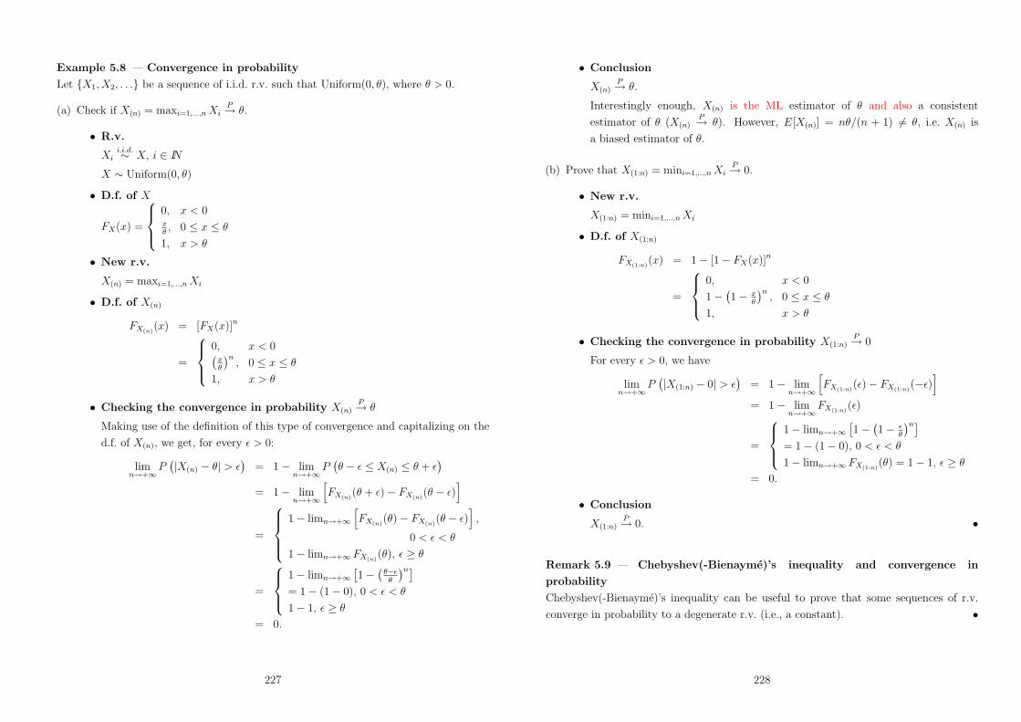
Example 5.8 — Convergence in probability
Let {X1, X2, . . .} be a sequence of i.i.d. r.v. such that Uniform(0, +), where + > 0.
(a) Check if X(n) = maxi=1,...,n XiP4 +.
• R.v.
Xii.i.d./ X, i " IN
X / Uniform(0, +)
• D.f. of X
FX(x) =
)*+
*,
0, x < 0x) , 0 ' x ' +
1, x > +
• New r.v.
X(n) = maxi=1,...,n Xi
• D.f. of X(n)
FX(n)(x) = [FX(x)]n
=
)*+
*,
0, x < 0-x)
.n, 0 ' x ' +
1, x > +
• Checking the convergence in probability X(n)P4 +
Making use of the definition of this type of convergence and capitalizing on the
d.f. of X(n), we get, for every % > 0:
limn&+!
P-|X(n) ! +| > %
.= 1! lim
n&+!P
-+ ! % ' X(n) ' + + %
.
= 1! limn&+!
GFX(n)
(+ + %)! FX(n)(+ ! %)
H
=
)**+
**,
1! limn&+!
GFX(n)
(+)! FX(n)(+ ! %)
H,
0 < % < +
1! limn&+! FX(n)(+), % - +
=
)*+
*,
1! limn&+!/1!
-)$*)
.n0
= 1! (1! 0), 0 < % < +
1! 1, % - +
= 0.
227
• Conclusion
X(n)P4 +.
Interestingly enough, X(n) is the ML estimator of + and also a consistent
estimator of + (X(n)P4 +). However, E[X(n)] = n+/(n + 1) &= +, i.e. X(n) is
a biased estimator of +.
(b) Prove that X(1:n) = mini=1,...,n XiP4 0.
• New r.v.
X(1:n) = mini=1,...,n Xi
• D.f. of X(1:n)
FX(1:n)(x) = 1! [1! FX(x)]n
=
)*+
*,
0, x < 0
1!-1! x
)
.n, 0 ' x ' +
1, x > +
• Checking the convergence in probability X(1:n)P4 0
For every % > 0, we have
limn&+!
P-|X(1:n) ! 0| > %
.= 1! lim
n&+!
GFX(1:n)
(%)! FX(1:n)(!%)
H
= 1! limn&+!
FX(1:n)(%)
=
)*+
*,
1! limn&+!/1!
-1! *
)
.n0
= 1! (1! 0), 0 < % < +
1! limn&+! FX(1:n)(+) = 1! 1, % - +
= 0.
• Conclusion
X(1:n)P4 0. •
Remark 5.9 — Chebyshev(-Bienayme)’s inequality and convergence in
probability
Chebyshev(-Bienayme)’s inequality can be useful to prove that some sequences of r.v.
converge in probability to a degenerate r.v. (i.e., a constant). •
228

Example 5.10 — Chebyshev(-Bienayme)’s inequality and convergence in
probability
Let {X1, X2, . . .} be a sequence of r.v. such that Xn / Gamma(n, n), n " IN . Prove that
XnP4 1, by making use of Chebyshev(-Bienayme)’s inequality.
• R.v.
Xn / Gamma(n, n), n " IN
E(Xn) = nn = 1
V (Xn) = nn2 = 1
n
• Checking the convergence in probability XnP4 1
The application of the definition of this type of convergence and Chebyshev(-
Bienayme)’s inequality leads to
limn&+!
P (|Xn ! 1| > %) = limn&+!
P
"|Xn ! E(Xn)| - %K
V (Xn)
KV (Xn)
$
' limn&+!
1'
*+1n
(2
=1
%2lim
n&+!
1
n= 0,
for every % > 0.
• Conclusion
XnP4 1. •
Exercise 5.11 — Chebyshev(-Bienayme)’s inequality and convergence in
probability
Prove that X(n) = maxi=1,...,n Xi, where Xi /i.i.d. Uniform(0, +), is a consistent estimator
of + > 0, by using Chebyshev(-Bienayme)’s inequality and the fact that E[X(n)] = nn+1 +
and V [X(n)] = n(n+2)(n+1)2 +2. •
229
Exercise 5.12 — Convergence in probability
Let {X1, X2, . . .} be a sequence of r.v. such that Xn / Bernoulli( 1n), n " IN .
(a) Show that XnP4 0, by obtaining P ({|Xn| > %}), for 0 < % < 1 and % - 1 (Rohatgi,
1976, pp. 243–244, Example 5).
(b) Verify that E(Xkn) 4 E(Xk), where k " IN and X
d= 0. •
Exercise 5.13 — Convergence in probability does not imply convergence of
kth. moments
Let {X1, X2, . . .} be a sequence of r.v. such that Xnd= n) Bernoulli( 1
n), n " IN , i.e.
P ({Xn = x}) =
)*+
*,
1! 1n , x = 0
1n , x = n
0, otherwise.
(5.4)
Prove that XnP4 0, however E(Xk
n) &4 E(Xk), where k " IN and the r.v. X is degenerate
at 0 (Rohatgi, 1976, p. 247, Remark 3). •
Motivation 5.14 — Convergence in quadratic mean and in L1
We have just seen that convergence in probability does not imply the convergence of
moments, namely of orders 2 or 1. •
Definition 5.15 — Convergence in quadratic mean or in L2 (Karr, 1993, p. 136)
Let X, X1, X2, . . . belong to L2. Then the sequence of r.v. {X1, X2, . . .} is said to converge
to X in quadratic mean (or in L2) — denoted by Xnq.m.4 X (or Xn
L2
4 X) — if
limn&+!
E/(Xn !X)2
0= 0. (5.5)
•
Exercise 5.16 — Convergence in quadratic mean
Let {X1, X2, . . .} be a sequence of r.v. such that Xn / Bernoulli-
1n
..
Prove that Xnq.m.4 X, where the r.v. X is degenerate at 0 (Rohatgi, 1976, p. 247,
Example 6). •
Exercise 5.17 — Convergence in quadratic mean (bis)
Let {X1, X2, . . .} be a sequence of r.v. with P-E
Xn = ± 1n
F .= 1
2 .
Prove that Xnq.m.4 X, where the r.v. X is degenerate at 0 (Rohatgi, 1976, p. 252,
Example 11). •
230

Exercise 5.18 — Convergence in quadratic mean implies convergence of 2nd.
moments (Karr, 1993, p. 158, Exercise 5.6(a))
Show that Xnq.m.4 X . E(X2
n) 4 E(X2) (Rohatgi, 1976, p. 248, proof of Theorem 8). •
Exercise 5.19 — Convergence in quadratic mean of partial sums (Karr, 1993, p.
159, Exercise 5.11)
Let X1, X2, . . . be pairwise uncorrelated r.v. with mean zero and partial sums
Sn =!n
i=1 Xi.
Prove that if there is a constant c such that V (Xi) ' c, for every i, thenSnn"
q.m.4 0 for all $ > 12 . •
Definition 5.20 — Convergence in mean or in L1 (Karr, 1993, p. 136)
Let X, X1, X2, . . . belong to L1. Then the sequence of r.v. {X1, X2, . . .} is said to converge
to X in mean (or in L1) — denoted by XnL1
4 X — if
limn&+!
E (|Xn !X|) = 0. (5.6)
•
Exercise 5.21 — Convergence in mean implies convergence of 1st. moments
(Karr, 1993, p. 158, Exercise 5.6(b))
Prove that XnL1
4 X . E(Xn) 4 E(X) (Rohatgi, 1976, p. 248, proof Theorem 8). •
231
5.1.2 Convergence in distribution
Motivation 5.22 — Convergence in distribution
(http://en.wikipedia.org/wiki/Convergence of random variables)
Convergence in distribution is very frequently used in practice, most often it arises from
the application of the central limit theorem. •
Definition 5.23 — Convergence in distribution (Karr, 1993, p. 136; Rohatgi, 1976,
pp. 240–1)
The sequence of r.v. {X1, X2, . . .} converges to X in distribution — denoted by Xnd4 X
— if
limn&+!
FXn(x) = FX(x), (5.7)
for all x at which FX is continuous. •
Remarks 5.24 — Convergence in distribution
(http://en.wikipedia.org/wiki/Convergence of random variables; Karr, 1993, p. 136;
Rohatgi, 1976, p. 242)
• With this mode of convergence, we increasingly expect to see the next r.v. in a
sequence of r.v. becoming better and better modeled by a given d.f., as seen in
exercises 5.25 and 5.26.
• It must be noted that it is quite possible for a given sequence of d.f. to converge to
a function that is not a d.f., as shown in Example 5.27 and Exercise 5.28.
• The requirement that only the continuity points of FX should be considered is
essential, as we shall see in exercises 5.29 and 5.30.
• The convergence in distribution does not imply the convergence of corresponding
p.(d.)f., as shown in Exercise 5.32. Sequences of absolutely continuous r.v. that
converge in distribution to discrete r.v. (and vice-versa) are obvious illustrations, as
shown in examples 5.31 and 5.33. •
Exercise 5.25 — Convergence in distribution
Let X1, X2, . . . , Xn be i.i.d. r.v. with common p.d.f.
f(x) =
71) , 0 < x < +
0, otherwise,(5.8)
232

where 0 < + < +,, and X(n) = max1,...,n Xi.
Show that X(n)d4 + (Rohatgi, 1976, p. 241, Example 2). •
Exercise 5.26 — Convergence in distribution (bis)
Let:
• {X1, X2, . . .} be a sequence of r.v. such that Xn / Bernoulli(pn), n = 1, 2, . . .;
• X / Bernoulli(p).
Prove that Xnd4 X i" pn 4 p. •
Example 5.27 — A sequence of d.f. converging to a non d.f. (Murteira, 1979, pp.
330–331)
Let {X1, X2, . . .} be a sequence of r.v. with d.f.
FXn(x) =
)*+
*,
0, x < !nx+n2n , !n ' x < n
1, x - n.
(5.9)
Please note that limn&+! FXn(x) = 12 , x " IR, as suggested by the graph below with some
terms of the sequence of d.f., for n = 1, 103, 106 (from top to bottom):
!1000 !500 500 1000
0.2
0.4
0.6
0.8
1.0
Consequently, the limit of the sequence of d.f. is not itself a d.f. •
Exercise 5.28 — A sequence of d.f. converging to a non d.f.
Consider the sequence of d.f.
FXn(x) =
70, x < n
1, x - n,(5.10)
where FXn(x) is the d.f. of the r.v. Xn degenerate at x = n.
Verify that FXn(x) converges to a function (that is identically equal to 0!!!) which is
not a d.f. (Rohatgi, 1976, p. 241, Example 1). •
233
Exercise 5.29 — The requirement that only the continuity points of FX should
be considered is essential
Let Xn / Uniform-
12 !
1n , 1
2 + 1n
.and X be a r.v. degenerate at 1
2 .
(a) Prove that Xnd4 X (Karr, 1993, p. 142).
(b) Verify that FXn
-12
.= 1
2 for each n, and these values do not converge to FX
-12
.= 1.
Is there any contradiction with the convergence in distribution previously proved?
(Karr, 1993, p. 142.) •
Exercise 5.30 — The requirement that only the continuity points of FX should
be considered is essential (bis)
Let Xn / Uniform-0, 1
n
.and X a r.v. degenerate at 0.
Prove that Xnd4 X, even though FXn(0) = 0, for all n, and FX(0) = 1,
that is, the convergence of d.f. fails at the point x = 0 where FX is discontinuous
(http://en.wikipedia.org/wiki/Convergence of random variables). •
Example 5.31 — Convergence in distribution does not imply convergence of
corresponding p.(d.)f. (Murteira, 1979, p. 331)
Let {X1, X2, . . .} be a sequence of r.v. such that Xn / Normal-0, 1
n2
..
An analysis of the representation of some terms of the sequence of d.f. (e.g. n =
1, 10, 50, from left to right in the following graph) and the notion of convergence in
distribution leads us to conclude that Xnd4 X, where X
d= 0, even though
limn&+!
FXn(0) = limn&+!
#
O
P0! 031n2
Q
R = #(0) =1
2
!3 !2 !1 1 2 3
0.2
0.4
0.6
0.8
1.0
234
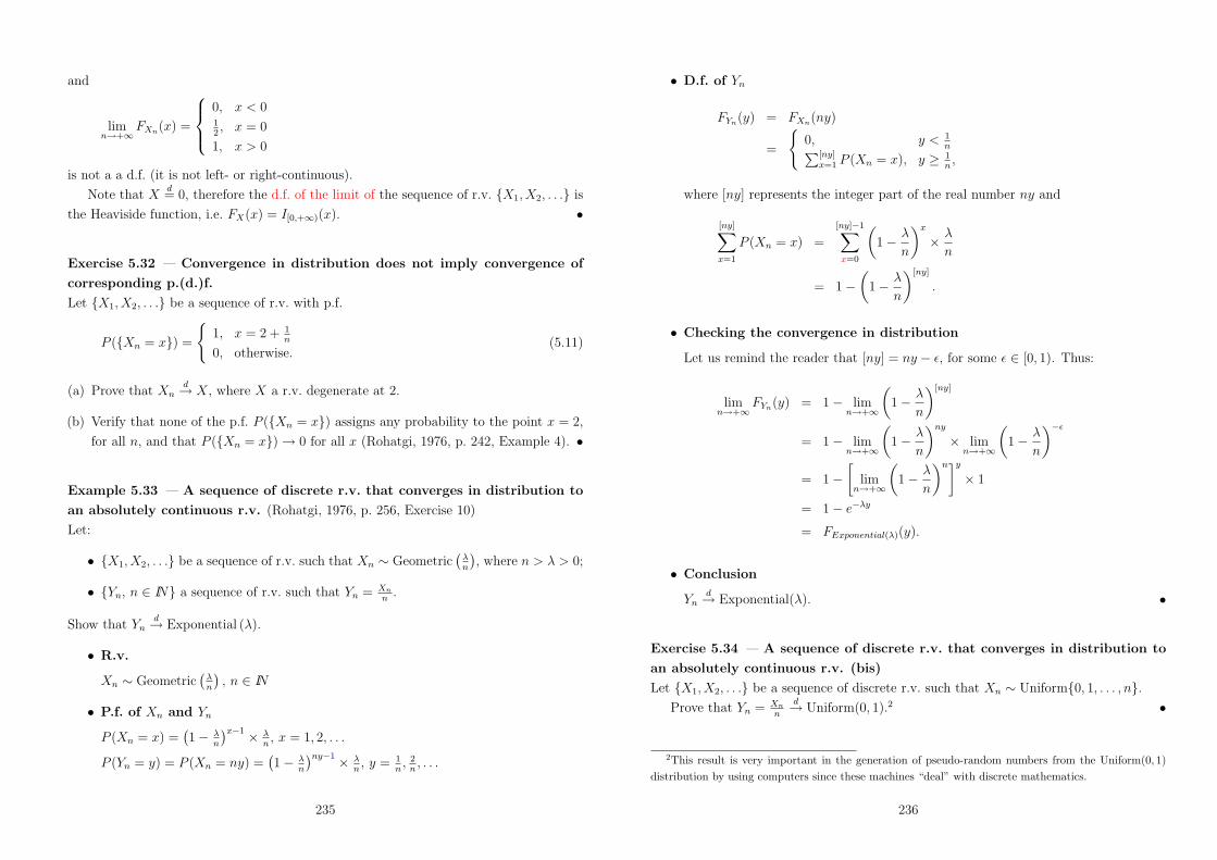
and
limn&+!
FXn(x) =
)*+
*,
0, x < 012 , x = 0
1, x > 0
is not a a d.f. (it is not left- or right-continuous).
Note that Xd= 0, therefore the d.f. of the limit of the sequence of r.v. {X1, X2, . . .} is
the Heaviside function, i.e. FX(x) = I[0,+!)(x). •
Exercise 5.32 — Convergence in distribution does not imply convergence of
corresponding p.(d.)f.
Let {X1, X2, . . .} be a sequence of r.v. with p.f.
P ({Xn = x}) =
71, x = 2 + 1
n
0, otherwise.(5.11)
(a) Prove that Xnd4 X, where X a r.v. degenerate at 2.
(b) Verify that none of the p.f. P ({Xn = x}) assigns any probability to the point x = 2,
for all n, and that P ({Xn = x}) 4 0 for all x (Rohatgi, 1976, p. 242, Example 4). •
Example 5.33 — A sequence of discrete r.v. that converges in distribution to
an absolutely continuous r.v. (Rohatgi, 1976, p. 256, Exercise 10)
Let:
• {X1, X2, . . .} be a sequence of r.v. such that Xn / Geometric-
"n
., where n > & > 0;
• {Yn, n " IN} a sequence of r.v. such that Yn = Xnn .
Show that Ynd4 Exponential (&).
• R.v.
Xn / Geometric-
"n
., n " IN
• P.f. of Xn and Yn
P (Xn = x) =-1! "
n
.x$1 ) "n , x = 1, 2, . . .
P (Yn = y) = P (Xn = ny) =-1! "
n
.ny$1 ) "n , y = 1
n , 2n , . . .
235
• D.f. of Yn
FYn(y) = FXn(ny)
=
70, y < 1
n![ny]x=1 P (Xn = x), y - 1
n ,
where [ny] represents the integer part of the real number ny and
[ny]%
x=1
P (Xn = x) =[ny]$1%
x=0
'1! &
n
(x
) &
n
= 1!'
1! &
n
([ny]
.
• Checking the convergence in distribution
Let us remind the reader that [ny] = ny ! %, for some % " [0, 1). Thus:
limn&+!
FYn(y) = 1! limn&+!
'1! &
n
([ny]
= 1! limn&+!
'1! &
n
(ny
) limn&+!
'1! &
n
($*
= 1!I
limn&+!
'1! &
n
(nJy
) 1
= 1! e$"y
= FExponential(")(y).
• Conclusion
Ynd4 Exponential(&). •
Exercise 5.34 — A sequence of discrete r.v. that converges in distribution to
an absolutely continuous r.v. (bis)
Let {X1, X2, . . .} be a sequence of discrete r.v. such that Xn / Uniform{0, 1, . . . , n}.Prove that Yn = Xn
n
d4 Uniform(0, 1).2 •
2This result is very important in the generation of pseudo-random numbers from the Uniform(0, 1)distribution by using computers since these machines “deal” with discrete mathematics.
236

The following table condenses the definitions of convergence of sequences of r.v.
Mode of convergence Assumption Defining condition
Xna.s.4 X (almost sure) — P ({w : Xn(!) 4 X(!)}) = 1
XnP4 X (in probability) — P ({|Xn !X| > '}) 4 0, for all ' > 0
Xnq.m4 X (in quadratic mean) X, X1, X2, . . . " L2 E
/(Xn !X)2
04 0
XnL1
4 X (in L1) X, X1, X2, . . . " L1 E (|Xn !X|) 4 0
Xnd4 X (in distribution) — FXn(x) 4 FX(x), at continuity points x of FX
Exercise 5.35 — Modes of convergence and uniqueness of limit (Karr, 1993, p.
158, Exercise 5.1)
Prove that for all five forms of convergence the limit is unique. In particular:
(a) if Xn,4 X and Xn
,4 Y , where @ = a.s., P, q.m., L1, then Xa.s.= Y ;
(b) if Xnd4 X and Xn
d4 Y , then Xd= Y ; •
Exercise 5.36 — Modes of convergence and the vector space structure of the
family of r.v. (Karr, 1993, p. 158, Exercise 5.2)
Prove that, for @ = a.s., P, q.m., L1,
Xn,4 X 2 Xn !X
,4 0, (5.12)
i.e. the four function-based forms of convergence are compatible with the vector space
structure of the family of r.v. •
237
5.1.3 Alternative criteria
The definition of almost sure convergence and its verification are far from trivial. More
tractable criteria have to be stated...
Proposition 5.37 — Relating almost sure convergence and convergence in
probability (Karr, 1993, p. 137; Rohatgi, 1976, p. 249)
Xna.s.4 X i"
(% > 0, limn&+!
P
'Lsupk)n
|Xk !X| > %
M(= 0, (5.13)
i.e.
Xna.s.4 X 2 Yn = sup
k)n|Xk !X| P4 0. (5.14)
•
Remarks 5.38 — Relating almost sure convergence and convergence in
probability (Karr, 1993, p. 137; Rohatgi, 1976, p. 250, Remark 6)
• Proposition 5.37 states an equivalent form of almost sure convergence that
illuminates its relationship to convergence in probability.
• Xna.s.4 0 means that,
(%, / > 0, An0 " IN : P
'Lsupk)n0
|Xk| > %
M(< /. (5.15)
Indeed, we can write, equivalently, that
limn&+!
P
"#
k)n
{|Xk| > %}$
= 0, (5.16)
for % > 0 arbitrary. •
Exercise 5.39 — Relating almost sure convergence and convergence in
probability
Prove Proposition 5.37 (Karr, 1993, p. 137; Rohatgi, 1976, p. 250). •
238

Exercise 5.40 — Relating almost sure convergence and convergence in
probability (bis)
Let {X1, X2, . . .} be a sequence of r.v. with P-E
Xn = ± 1n
F .= 1
2 .
Prove that Xna.s.4 X, where the r.v. X is degenerate at 0, by using (5.16) (Rohatgi,
1976, p. 252). •
Theorem 5.41 — Cauchy criterion (Rohatgi, 1976, p. 270)
Xna.s.4 X 2 lim
n&+!P
'Lsupm
|Xn+m !Xn| ' %
M(= 1, (% > 0. (5.17)
•
Exercise 5.42 — Cauchy criterion
Prove Theorem 5.41 (Rohatgi, 1976, pp. 270–2). •
Definition 5.43 — Complete convergence (Karr, 1993, p. 138)
The sequence of r.v. {X1, X2, . . .} is said to converge completely to X if
+!%
n=1
P ({|Xn !X| > %} ) < +,, (5.18)
for every % > 0. •
The next results relate complete convergence, which is stronger than almost sure
convergence, and sometimes more convenient to establish (Karr, 1993, p. 137).
Proposition 5.44 — Relating almost sure convergence and complete
convergence (Karr, 1993, p. 138)
+!%
n=1
P ({|Xn !X| > %} ) < +,, (% > 0 . Xna.s.4 X. (5.19)
•
Remark 5.45 — Relating almost sure convergence and complete convergence
(Karr, 1993, p. 138)
XnP4 X i" the probabilities P ({|Xn !X| > %} ) converge to zero, while Xn
a.s.4 X if (but
not only if) the convergence of probabilities P ({|Xn !X| > %} ) is fast enough that their
sum,!+!
n=1 P ({|Xn !X| > %} ), is finite. •
239
Exercise 5.46 — Relating almost sure convergence and complete convergence
Show Proposition 5.44, by using the (1st.) Borel-Cantelli lemma (Karr, 1993, p. 138). •
Theorem 5.47 — Almost sure convergence of a sequence of independent r.v.
(Rohatgi, 1976, p. 265)
Let {X1, X2, . . .} be a sequence of independent r.v. Then
Xna.s.4 0 2
+!%
n=1
P ({|Xn| > %} ) < +,, (% > 0. (5.20)
•
Exercise 5.48 — Almost sure convergence of a sequence of independent r.v.
(a) Prove Theorem 5.47 (Rohatgi, 1976, pp. 265–6).
(b) Use Theorem 5.47 to solve Exercise 5.40. •
The definition of convergence in distribution is cumbersome because of the proviso
regarding continuity points of the limit d.f. FX . An alternative criterion follows.
Theorem 5.49 — Alternative criterion for convergence in distribution (Karr,
1993, p. 138)
Let C be the set of bounded, continuous functions f : IR 4 IR. Then
Xnd4 X 2 E[f(Xn)] 4 E[f(X)], ( f " C. (5.21)
•
Remark 5.50 — Alternative criterion for convergence in distribution (Karr,
1993, p. 138)
Theorem 5.49 provides a criterion for convergence in distribution which is superior to the
definition of convergence in distribution in that one needs not to deal with continuity
points of the limit d.f. •
Exercise 5.51 — Alternative criterion for convergence in distribution
Prove Theorem 5.49 (Karr, 1993, pp. 138–139). •
Since in the proof of Theorem 5.49 the continuous functions used to approximate
indicator functions can be taken to be arbitrarily smooth we can add a su$cient condition
that guarantees convergence in distribution.
240

Corollary 5.52 — Su"cient condition for convergence in distribution (Karr,
1993, p. 139)
Let:
• k be a fixed non-negative integer;
• C(k) be the space of bounded, k!times uniformly continuously di"erentiable
functions f : IR 4 IR.
Then
E[f(Xn)] 4 E[f(X)], ( f " C(k) . Xnd4 X. (5.22)
•
The next table summarizes the alternative criteria and su$cient conditions for almost
sure convergence and convergence in distribution of sequences of r.v.
Alternative criterion or su!cient condition Mode of convergence
(' > 0, limn$+" P-E
supk&n |Xk !X| > 'F.
= 0 2 Xna.s.4 X
Yn = supk&n |Xk !X| P4 0 2 Xna.s.4 X
limn$+" P ({supm |Xn+m !Xn| ' '}) = 1, (' > 0 2 Xna.s.4 X
!+"n=1 P ({|Xn !X| > '} ) < +,, ( ' > 0 . Xn
a.s.4 X!+"
n=1 P ({|Xn| > '} ) < +,, ( ' > 0 2 Xna.s.4 0
E[f(Xn)] 4 E[f(X)], ( f " C 2 Xnd4 X
E[f(Xn)] 4 E[f(X)], ( f " C(k) for a fixed k " IN0 . Xnd4 X
We should also add that Grimmett and Stirzaker (2001, p. 310) state that if XnP4 X
and P ({|Xn| ' k}) = 1, for all n and some k, then XnLr
4 X, for all r - 1,3 namely
Xnq.m.4 X (which in turn implies Xn
L1
4 X).
3Let X, X1, X2, . . . belong to Lr (r - 1). Then the sequence of r.v. {X1, X2, . . .} is said to convergeto X in Lr) — denoted by Xn
Lr
4 X — if limn$+"E (|Xn !X|r) = 0 (Grimmett and Stirzaker, 2001,p. 308).
241
5.2 Relationships among the modes of convergence
Given the plethora of modes of convergence, it is natural to inquire how they can be
always related or hold true in the presence of additional assumptions (Karr, 1993, pp. 140
and 142).
5.2.1 Implications always valid
Proposition 5.53 — Almost sure convergence implies convergence in
probability (Karr, 1993, p. 140; Rohatgi, 1976, p. 250)
Xna.s.4 X . Xn
P4 X. (5.23)
•
Exercise 5.54 — Almost sure convergence implies convergence in probability
Show Proposition 5.53 (Karr, 1993, p. 140; Rohatgi, 1976, p. 251). •
Proposition 5.55 — Convergence in quadratic mean implies convergence in L1
(Karr, 1993, p. 140)
Xnq.m.4 X . Xn
L1
4 X. (5.24)
•
Exercise 5.56 — Convergence in quadratic mean implies convergence in L1
Prove Proposition 5.55, by applying Cauchy-Schwarz’s inequality (Karr, 1993, p. 140). •
Proposition 5.57 — Convergence in L1 implies convergence in probability
(Karr, 1993, p. 141)
XnL1
4 X . XnP4 X. (5.25)
•
Exercise 5.58 — Convergence in L1 implies convergence in probability
Prove Proposition 5.57, by using Chebyshev’s inequality (Karr, 1993, p. 141). •
Proposition 5.59 — Convergence in probability implies convergence in
distribution (Karr, 1993, p. 141)
XnP4 X . Xn
d4 X. (5.26)
•
242

Exercise 5.60 — Convergence in probability implies convergence in
distribution
Show Proposition 5.59, (Karr, 1993, p. 141). •
Figure 5.1 shows that convergence in distribution is the weakest form of convergence,
since it is implied by all other types of convergence studied so far.
Xnq.m.4 X . Xn
L1
4 X
.Xn
P4 X . Xnd4 X
.Xn
a.s.4 X
Figure 5.1: Implications always valid between modes of convergence.
Grimmett and Stirzaker (2001, p. 314) refer that convergence in distribution is the
weakest form of convergence for two reasons: it only involves d.f. and makes no reference
to an underlying probability space.4 However, convergence in distribution has an useful
representation in terms of almost sure convergence, as stated in the next theorem.
Theorem 5.61 — Skorokhod’s representation theorem (Grimmett and Stirzaker,
2001, p. 314)
Let {X1, X2, . . .} be a sequence of r.v., {F1, F2, . . .} the associated sequence of d.f. and X
be a r.v. with d.f. F . If Xnd4 X then there is a probability space (!-,F -, P -) and r.v.
{Y1, Y2, . . .} and Y mapping !- into IR such that {Y1, Y2, . . .} and Y have d.f. {F1, F2, . . .}and F and Yn
a.s.4 Y . •
Remark 5.62 — Skorokhod’s representation theorem (Grimmett and Stirzaker,
2001, p. 315)
Although Xn may fail to converge to X in any mode than in distribution, there is a
sequence of r.v. {Y1, Y2, . . .} such that Yn is identically distributed to Xn, for every n,
which converges almost surely to a “copy” of X. •
4Let us remind the reader that that there is an equivalent formulation of convergence in distributionwhich involves d.f. alone: the sequence of d.f. {F1, F2, . . .} converges to the d.f. F , if limn$+" Fn(x) =F (x) at each point x where F is continuous (Grimmett and Stirzaker, 2001, p. 190).
243
5.2.2 Counterexamples
Counterexamples to all implications among the modes of convergence (and more!) are
condensed in Figure 5.2 and presented by means of several exercises.
Xnq.m.4 X &B Xn
L1
4 X
&BXn
P4 X &B Xnd4 X
&BXn
a.s.4 X
Figure 5.2: Counterexamples to implications among the modes of convergence.
Before proceeding with exercises, recall exercises 5.4 and 5.12 which pertain to the
sequence of r.v. {X1, X2, . . .}, where Xn / Bernoulli( 1n), n " IN . In the first exercise
we proved that Xn &a.s.4 0, whereas in the second one we concluded that Xn
P4 0. Thus,
combining these results we can state that XnP4 0 &. Xn
a.s.4 0.
Exercise 5.63 — Almost sure convergence does not imply convergence in
quadratic mean
Let {X1, X2, . . .} be a sequence of r.v. such that
P ({Xn = x}) =
)*+
*,
1! 1n , x = 0
1n , x = n
0, otherwise.
(5.27)
Prove that Xna.s.4 0, and, hence, Xn
P4 0 and Xnd4 0, but Xn &
L1
4 0 and Xn &q.m.4 0
(Karr, 1993, p. 141, Counterexample a)). •
Exercise 5.64 — Almost sure convergence does not imply convergence in
quadratic mean (bis)
Let {X1, X2, . . .} be a sequence of r.v. such that
P ({Xn = x}) =
)*+
*,
1! 1nr , x = 0
1nr , x = n
0, otherwise,
(5.28)
where r - 2.
Prove that Xna.s.4 0, but Xn &
q.m.4 0 for r = 2 (Rohatgi, 1976, p. 252, Example 10). •
244
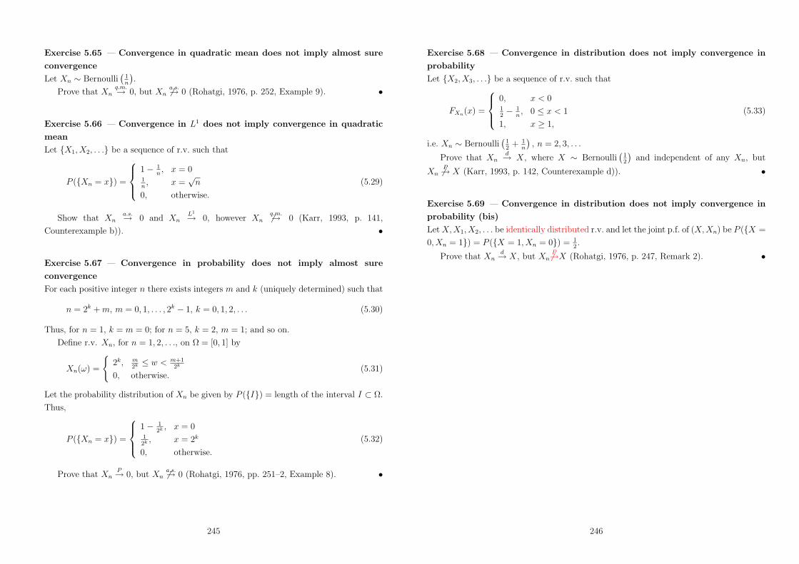
Exercise 5.65 — Convergence in quadratic mean does not imply almost sure
convergence
Let Xn / Bernoulli-
1n
..
Prove that Xnq.m.4 0, but Xn &
a.s.4 0 (Rohatgi, 1976, p. 252, Example 9). •
Exercise 5.66 — Convergence in L1 does not imply convergence in quadratic
mean
Let {X1, X2, . . .} be a sequence of r.v. such that
P ({Xn = x}) =
)*+
*,
1! 1n , x = 0
1n , x =
+n
0, otherwise.
(5.29)
Show that Xna.s.4 0 and Xn
L1
4 0, however Xn &q.m.4 0 (Karr, 1993, p. 141,
Counterexample b)). •
Exercise 5.67 — Convergence in probability does not imply almost sure
convergence
For each positive integer n there exists integers m and k (uniquely determined) such that
n = 2k + m, m = 0, 1, . . . , 2k ! 1, k = 0, 1, 2, . . . (5.30)
Thus, for n = 1, k = m = 0; for n = 5, k = 2, m = 1; and so on.
Define r.v. Xn, for n = 1, 2, . . ., on ! = [0, 1] by
Xn(!) =
72k, m
2k ' w < m+12k
0, otherwise.(5.31)
Let the probability distribution of Xn be given by P ({I}) = length of the interval I # !.
Thus,
P ({Xn = x}) =
)*+
*,
1! 12k , x = 0
12k , x = 2k
0, otherwise.
(5.32)
Prove that XnP4 0, but Xn &
a.s.4 0 (Rohatgi, 1976, pp. 251–2, Example 8). •
245
Exercise 5.68 — Convergence in distribution does not imply convergence in
probability
Let {X2, X3, . . .} be a sequence of r.v. such that
FXn(x) =
)*+
*,
0, x < 012 !
1n , 0 ' x < 1
1, x - 1,
(5.33)
i.e. Xn / Bernoulli-
12 + 1
n
., n = 2, 3, . . .
Prove that Xnd4 X, where X / Bernoulli
-12
.and independent of any Xn, but
Xn &P4 X (Karr, 1993, p. 142, Counterexample d)). •
Exercise 5.69 — Convergence in distribution does not imply convergence in
probability (bis)
Let X, X1, X2, . . . be identically distributed r.v. and let the joint p.f. of (X, Xn) be P ({X =
0, Xn = 1}) = P ({X = 1, Xn = 0}) = 12 .
Prove that Xnd4 X, but Xn &
P4X (Rohatgi, 1976, p. 247, Remark 2). •
246

5.2.3 Implications of restricted validity
Proposition 5.70 — Convergence in distribution to a constant implies
convergence in probability (Karr, 1993, p. 140; Rohatgi, 1976, p. 246)
Let {X1, X2, . . .} be a sequence of r.v. and c " IR. Then
Xnd4 c . Xn
P4 c. (5.34)
•
Remark 5.71 — Convergence in distribution to a constant is equivalent to
convergence in probability (Rohatgi, 1976, p. 246)
If we add to the previous result the fact that XnP4 c . Xn
d4 c, we can conclude that
XnP4 c 2 Xn
d4 c. (5.35)
•
Exercise 5.72 — Convergence in distribution to a constant implies convergence
in probability
Show Proposition 5.70 (Karr, 1993, p. 142). •
Exercise 5.73 — Convergence in distribution to a constant implies convergence
in probability (bis)
Let (X1, . . . , Xn) be a random vector where Xi are i.i.d. r.v. with common p.d.f.
fX(x) = +x$2 ) I[),+!)(x),
where + " IR+.
(a) After having proved that
FX(1:n)(x) = P
'min
i=1,...,nXi ' x
(= [1! (+/x)n]) I[),+!)(x), (5.36)
derive the following result: X(1:n)d4 +.
(b) Is X(1:n) a consistent estimator of +? •
Definition 5.74 — Uniform integrability (Karr, 1993, p. 142)
A sequence of r.v. {X1, X2, . . .} is uniformly integrable if Xn " L1 for each n " IN and if
lima&+!
supn
E(|Xn|; {|Xn| > a}) = 0. (5.37)
Recall that the expected value of a r.v. X over an event A is given by E(X; A) = E(X )1A). •
247
Proposition 5.75 — Alternative criterion for uniform integrability (Karr, 1993,
p. 143)
A sequence of r.v. {X1, X2, . . .} is uniformly integrable i"
• supn E(|Xn|) < +, and
• {X1, X2, . . .} is uniformly absolutely continuous: for each % > 0 there is ' > 0 such
that supn E(|Xn|; A) < % whenever P (A) > '. •
Proposition 5.76 — Combining convergence in probability and uniform
integrability is equivalent to convergence in L1 (Karr, 1993, p. 144)
Let X, X1, X2, . . . " L1. Then
XnP4 X and {X1, X2, . . .} is uniformly integrable 2 Xn
L1
4 X. (5.38)
•
Exercise 5.77 — Combining convergence in probability and uniform
integrability is equivalent to convergence in L1
Prove Proposition 5.76 (Karr, 1993, p. 144). •
Exercise 5.78 — Combining convergence in probability of the sequence of r.v.
and convergence of sequence of the means implies convergence in L1 (Karr,
1993, p. 160, Exercise 5.16)
Let X, X1, X2, . . . be positive r.v.
Prove that if XnP4 X and E(Xn) 4 E(X), then Xn
L1
4 X. •
Exercise 5.79 — Increasing character and convergence in probability
combined imply almost sure convergence (Karr, 1993, p. 160, Exercise 5.15)
Show that if X1 ' X2 ' . . . and XnP4 X, then Xn
a.s.4 X. •
Exercise 5.80 — Strictly decreasing and positive character and convergence
in probability combined imply almost sure convergence (Rohatgi, 1976, p. 252,
Theorem 13)
Let {X1, X2, . . .} be a strictly decreasing sequence of positive r.v.
Prove that if XnP4 0 then Xn
a.s.4 0. •
248
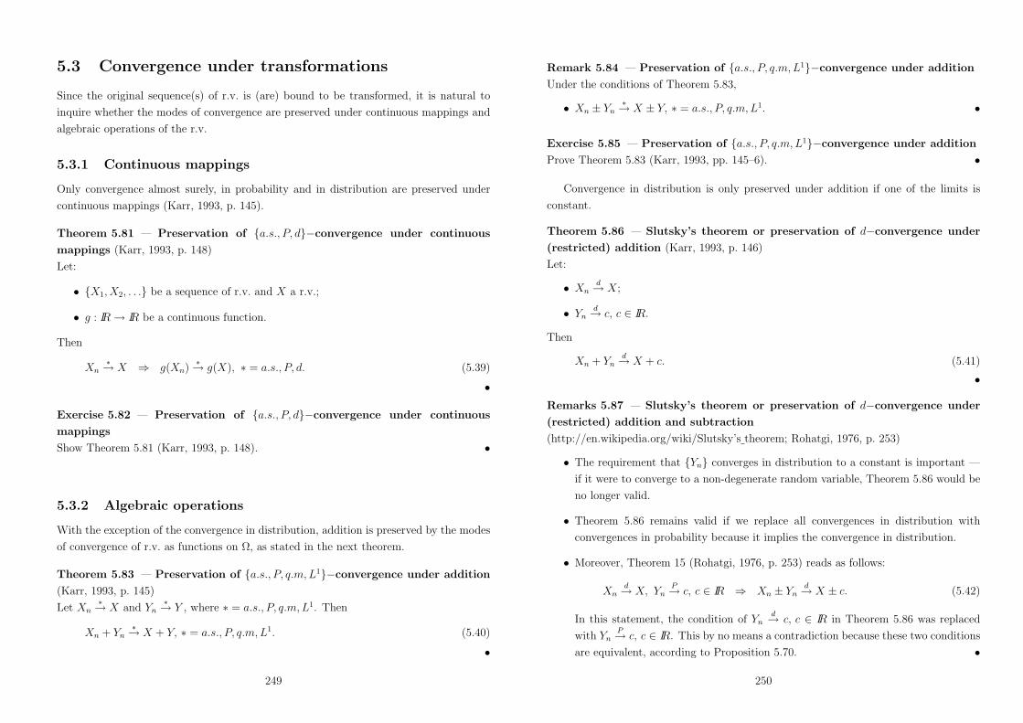
5.3 Convergence under transformations
Since the original sequence(s) of r.v. is (are) bound to be transformed, it is natural to
inquire whether the modes of convergence are preserved under continuous mappings and
algebraic operations of the r.v.
5.3.1 Continuous mappings
Only convergence almost surely, in probability and in distribution are preserved under
continuous mappings (Karr, 1993, p. 145).
Theorem 5.81 — Preservation of {a.s., P, d}!convergence under continuous
mappings (Karr, 1993, p. 148)
Let:
• {X1, X2, . . .} be a sequence of r.v. and X a r.v.;
• g : IR 4 IR be a continuous function.
Then
Xn,4 X . g(Xn)
,4 g(X), @ = a.s., P, d. (5.39)
•
Exercise 5.82 — Preservation of {a.s., P, d}!convergence under continuous
mappings
Show Theorem 5.81 (Karr, 1993, p. 148). •
5.3.2 Algebraic operations
With the exception of the convergence in distribution, addition is preserved by the modes
of convergence of r.v. as functions on !, as stated in the next theorem.
Theorem 5.83 — Preservation of {a.s., P, q.m, L1}!convergence under addition
(Karr, 1993, p. 145)
Let Xn,4 X and Yn
,4 Y , where @ = a.s., P, q.m, L1. Then
Xn + Yn,4 X + Y, @ = a.s., P, q.m, L1. (5.40)
•
249
Remark 5.84 — Preservation of {a.s., P, q.m, L1}!convergence under addition
Under the conditions of Theorem 5.83,
• Xn ± Yn,4 X ± Y, @ = a.s., P, q.m, L1. •
Exercise 5.85 — Preservation of {a.s., P, q.m, L1}!convergence under addition
Prove Theorem 5.83 (Karr, 1993, pp. 145–6). •
Convergence in distribution is only preserved under addition if one of the limits is
constant.
Theorem 5.86 — Slutsky’s theorem or preservation of d!convergence under
(restricted) addition (Karr, 1993, p. 146)
Let:
• Xnd4 X;
• Ynd4 c, c " IR.
Then
Xn + Ynd4 X + c. (5.41)
•
Remarks 5.87 — Slutsky’s theorem or preservation of d!convergence under
(restricted) addition and subtraction
(http://en.wikipedia.org/wiki/Slutsky’s theorem; Rohatgi, 1976, p. 253)
• The requirement that {Yn} converges in distribution to a constant is important —
if it were to converge to a non-degenerate random variable, Theorem 5.86 would be
no longer valid.
• Theorem 5.86 remains valid if we replace all convergences in distribution with
convergences in probability because it implies the convergence in distribution.
• Moreover, Theorem 15 (Rohatgi, 1976, p. 253) reads as follows:
Xnd4 X, Yn
P4 c, c " IR . Xn ± Ynd4 X ± c. (5.42)
In this statement, the condition of Ynd4 c, c " IR in Theorem 5.86 was replaced
with YnP4 c, c " IR. This by no means a contradiction because these two conditions
are equivalent, according to Proposition 5.70. •
250

Exercise 5.88 — Slutsky’s theorem or preservation of d!convergence under
(restricted) addition
Prove Theorem 5.86 (Karr, 1993, p. 146; Rohatgi, 1976, pp. 253–4). •
As for the product, almost sure convergence and convergence in probability are
preserved.
Theorem 5.89 — Preservation of {a.s., P}!convergence under product (Karr,
1993, p. 147)
Let Xn,4 X and Yn
,4 Y , where @ = a.s., P . Then
Xn ) Yn,4 X ) Y, @ = a.s., P. (5.43)
•
Exercise 5.90 — Preservation of {a.s., P}!convergence under product
Show Theorem 5.89 (Karr, 1993, p. 147).5 •
Theorem 5.91 — (Non)preservation of q.m.!convergence under product (Karr,
1993, p. 147)
Let Xnq.m.4 X and Yn
q.m.4 Y . Then
Xn ) YnL1
4 X ) Y. (5.44)
•
Remark 5.92 — (Non)preservation of q.m.!convergence under product (Karr,
1993, pp. 146–7)
Quadratic mean convergence of products does not hold in general, since X ) Y need not
belong to L2 when X and Y do:
Xnq.m.4 X, Yn
q.m.4 Y &. Xn ) Ynq.m.4 X ) Y. (5.45)
However, the product of r.v. in L2 belongs to L1, and L2 convergence of factors implies
L1 convergence of products. •
5Proposition 5.18 of Karr (1993, p. 144) may come handy to prove the result. This propositionreads as follows: the sequence of r.v. {X1, X2, . . .} converges in probability to X i" each subsequence{X1! , X2! , . . .} contains a further subsequence {X1!! , X2!! , . . .} such that Xn
a.s.4 X.
251
Exercise 5.93 — (Non)preservation of q.m.!convergence under product
Prove Theorem 5.91 (Karr, 1993, p. 147; Rohatgi, 1976, p. 254). •
Convergence in distribution is preserved under product, provided that one limit factor
is constant (Karr, 1993, p. 146).
Theorem 5.94 — Slutsky’s theorem (bis) or preservation of d!convergence
under (restricted) product (Karr, 1993, p. 147)
Let:
• Xnd4 X;
• Ynd4 c, c " IR.
Then
Xn ) Ynd4 X ) c. (5.46)
•
Remark 5.95 — Slutsky’s theorem or preservation of d!convergence under
(restricted) product (Rohatgi, 1976, p. 253)
Rohatgi (1976, p. 253, Theorem 15) also states that
Xnd4 X, Yn
P4 c, c " IR . Xn ) Ynd4 X ) c (5.47)
Xnd4 X, Yn
P4 c, c " IR\{0} . Xn
Yn
d4 X
c. (5.48)
(Discuss the validity of both results.) •
Preservation under...
Mode of convergence Continuous mapping Addition & Subtraction Producta.s.4 (almost sure) Yes Yes Yes
P4 (in probability) Yes Yes Yes
q.m.4 (in quadratic mean) No YesL1
4
L1
4 (in L1) No Yes Yes
d4 (in distribution) Yes RV' RV'
' Restricted validity (RV): one of the summands/factors has to converge in distribution to a constant
252

Exercise 5.96 — Slutsky’s theorem or preservation of d!convergence under
(restricted) product
Prove Theorem 5.94 (Karr, 1993, pp. 147–8). •
Example/Exercise 5.97 — Slutsky’s theorem or preservation of d!convergence
under (restricted) product
Consider the sequence of r.v. {X1, X2, . . .}, where Xni.i.d./ X and let Xn = 1
n
!ni=1 Xi and
S2n = 1
n$1
!ni=1(Xi ! Xn)2 be the sample mean and the variance of the first n r.v.
(a) Show that
Xn ! µ
Sn/+
nd4 Normal(0, 1), (5.49)
for any X " L4.
• R.v.
Xii.i.d./ X, i " IN
X : E(X) = µ, V (X) = #2 = µ2, E [(X ! µ)4] = µ4, which are finite
moments since X " L4.
• Auxiliary results
E(Xn) = µ
V (Xn) = #2
n = µ2
n
E(S2n) = #2 = µ2
V (S2n) =
-n
n$1
.2G
µ4$µ22
n ! 2(µ4$2µ22)
n2 + 2(µ4$3µ22)
n3
H(Murteira, 1980, p. 46).
• Asymptotic sample distribution of Xn$µSn/
%n
To show that Xn$µSn/
%n
d4 Normal(0, 1) it su$ces to note that
Xn ! µ
Sn/+
n=
Xn$µ#/%
n3S2
n#2
, (5.50)
prove that Xn$µ#/%
n
d4 Normal(0, 1) and3
S2n
#2
P4 1, and then apply Slutsky’s
theorem as stated in (5.48).
• Convergence in distribution of the numerator
It follows immediately from the Central Limit Theorem.6
6This well known theorem is thoroughly discussed by Karr (1993, pp. 190–196) and also in Section5.9.
253
• Convergence in probability of the denominator
By using the definition of convergence in probability and the Chebyshev(-
Bienayme)’s inequality, we get, for any % > 0:
limn&+!
P-|S2
n ! #2| > %.
= limn&+!
P
"DDS2
n ! E(S2n)
DD - %KV (S2
n)
KV (S2
n)
$
' limn&+!
1'
*+V (S2
n)
(2
=1
%2lim
n&+!V (S2
n)
= 0, (5.51)
i.e. S2n
P4 #2.
Finally, note that convergence in probability is preserved under continuous
mappings such as g(x) =K
x# , hence
S2n
P4 #2 .N
S2n
#2
P4N
#2
#2= 1. (5.52)
• ConclusionX$µS/%
n
d4 Normal(0, 1).
(b) Discuss the utility of this result. •
Exercise 5.98 — Slutsky’s theorem or preservation of d!convergence under
(restricted) division
Let Xii.i.d./ Normal(0, 1), i " IN .
Determine the limiting distribution of Wn = UnVn
, where
Un =
!ni=1 Xi+
n(5.53)
Vn =
!ni=1 X2
i
n, (5.54)
by proving that
Und4 Normal(0, 1) (5.55)
Vnd4 1 (5.56)
(Rohatgi, 1976, pp. 254, Example 12). •
254

Exercise 5.99 — Slutsky’s theorem or preservation of d!convergence under
(restricted) division (bis)
Let {X1, X2, . . .} a sequence of i.i.d. r.v. with common distribution Bernoulli(p) and Xn =1n
!ni=1 Xi the maximum likelihood estimator of p.
(a) Prove that
Xn ! p3Xn(1$Xn)
n
d4 Normal(0, 1). (5.57)
(b) Discuss the relevance of this convergence in distribution. •
255
5.4 Convergence of random vectors
Before defining modes of convergence of a sequence of random d!vectors we need two
recall the definition of norm of a vector.
Definition 5.100 — L2 (or Euclidean) and L1 norms of x (Karr, 1993, p. 149)
Let x " IRd and x(i) its ith component. Then
||x||L2 =
STTUd%
i=1
x(i)2 (5.58)
||x||L1 =d%
i=1
|x(i)| (5.59)
denote the L2 norm (or Euclidean norm) and the L1 norm of x, respectively. •
Remark 5.101 — L2 (or Euclidean) and L1 norms of x
(http://en.wikipedia.org/wiki/Norm mathematics0Definition)
On IRd, the intuitive notion of length of the vector x is captured by its L2 or Euclidean
norm: this gives the ordinary distance from the origin to the point x, a consequence of
the Pythagorean theorem.
The Euclidean norm is by far the most commonly used norm on IRd, but there are
other norms, such as the L1 norm on this vector space. •
Definition 5.102 — Four modes of convergence (as functions of !) of sequences
of random vectors (Karr, 1993, p. 149)
Let X, X1, X2, . . . be random d!vectors. Then the four modes of convergence Xn,4 X,
@ = a.s., P, q.m., L1 are natural extensions of their counterparts in the univariate case:
• Xna.s.4 X if P ({! : limn&+! ||Xn(!)!X(!)||L1= 0}) = 1;
• XnP4 X if limn&+! P ({||Xn !X||L1 > %}) = 0, for every % > 0;
• Xnq.m.4 X if limn&+!E (||Xn !X||L2) = 0;
• XnL1
4 X if limn&+!E (||Xn !X||L1) = 0. •
Proposition 5.103 — Alternative criteria for the four modes of convergence of
sequences of random vectors (Karr, 1993, p. 149)
Xn,4 X, @ = a.s., P, q.m., L1 i" the same kind of stochastic convergence holds for each
component, i.e. Xn(i),4 X(i), @ = a.s., P, q.m., L1, i = 1, . . . , d. •
256
Remark 5.104 — Convergence in distribution of a sequence of random vectors
(Karr, 1993, p. 149)
Due to the intractability of multi-dimension d.f., convergence in distribution — unlike
the four previous modes of convergence — has to be defined by taking advantage of the
alternative criterion for convergence in distribution stated in Theorem 5.49. •
Definition 5.105 — Convergence in distribution of a sequence of random
vectors
(Karr, 1993, p. 149)
Let X, X1, X2, . . . be random d!vectors. Then:
• Xnd4 X if E[f(Xn)] 4 E[f(X)], for all bounded, continuous functions f : IRd 4
IR. •
Proposition 5.106 — A su"cient condition for the convergence in distribution
of the components of a sequence of random vectors (Karr, 1993, p. 149)
Unlike the four previous modes of convergence, convergence in distribution of the
components of a sequence of random vectors is implied, but need not imply, convergence
in distribution of the sequence of random vectors:
Xnd4 X . (&B) Xn(i)
d4 X(i), (5.60)
for each i. •
A sequence of random vectors converges in distribution i" every linear combination
of their components converges in distribution; this result constitutes the Cramer-Wold
device.
Theorem 5.107 (Cramer-Wold device) — An alternative criterion for the
convergence in distribution of a sequence of random vectors (Karr, 1993, p.
150)
Let X, X1, X2, . . . be random d!vectors. Then
Xnd4 X 2 a2Xn =
d%
i=1
a(i))Xn(i)d4
d%
i=1
a(i))X(i) = a2X, (5.61)
for all a " IRd. •
Exercise 5.108 — An alternative criterion for the convergence in distribution
of a sequence of random vectors
Show Theorem 5.107 (Karr, 1993, p. 150). •
257
As with sequences of r.v., convergence almost surely, in probability and in distribution
are preserved under continuous mappings of sequences of random vectors.
Theorem 5.109 — Preservation of {a.s., P, d}!convergence under continuous
mappings of random vectors (Karr, 1993, p. 148)
Let:
• {X1, X2, . . .} be a sequence of random d!vectors and X a random d!vector;
• g : IRd 4 IRm be a continuous mapping of IRd into IRm.
Then
Xn,4 X . g(Xn)
,4 g(X), @ = a.s., P, d. (5.62)
•
258

5.5 Limit theorems for Bernoulli summands
Let {X1, X2, . . .} be a Bernoulli process with parameter p " (0, 1). In this section we
study the asymptotic behavior of the Bernoulli counting process {S1, S2, . . .}, where Sn =!n
i=1 Xi / Binomial(n, p).
5.5.1 Laws of large numbers for Bernoulli summands
Motivation 5.110 — Laws of large numbers
(http://en.wikipedia.org/wiki/Law of large numbers; Murteira, 1979, p. 313)
In probability theory, the law of large numbers (LLN) is a theorem that describes the
result of performing the same experiment a large number of times. According to the law,
the average of the results obtained from a large number of trials (e.g. Bernoulli trials)
should be close to the expected value, and will tend to become closer as more trials are
performed.
For instance, when a fair coin is flipped once, the expected value of the number of
heads is equal to one half. Therefore, according to the law of large numbers, the proportion
of heads in a large number of coin flips should be roughly one half, as depicted by the
next figure (where N stands for n).
This illustration suggests the following statement: Snn = Xn converges, in some sense, to
p = 12 . In fact, if we use Chebyshev(-Bienayme)’s inequality we can prove that
limn&+!
P
'LDDDDSn
n! p
DDDD > 1
M(= 0, (5.63)
that is, Snn
P4 p = 12 . (Show this result!) In addition, we can also prove that the proportion
of heads after n flips will almost surely converge to one half as n approaches infinity, i.e.,Snn
a.s.4 p = 12 . Similar convergences can be devised for the mean of n i.i.d. r.v.
The Indian mathematician Brahmagupta (598–668) and later the Italian
mathematician Gerolamo Cardano (1501–1576) stated without proof that the accuracies
of empirical statistics tend to improve with the number of trials. This was then formalized
as a law of large numbers (LLN).
259
The LLN was first proved by Jacob Bernoulli. It took him over 20 years to develop a
su$ciently rigorous mathematical proof which was published in his Ars Conjectandi (The
Art of Conjecturing) in 1713. He named this his Golden Theorem but it became generally
known as ”Bernoulli’s Theorem”. In 1835, S.D. Poisson further described it under the
name La loi des grands nombres (The law of large numbers). Thereafter, it was known
under both names, but the Law of large numbers is most frequently used.
Other mathematicians also contributed to refinement of the law, including Chebyshev,
Markov, Borel, Cantelli and Kolmogorov. These further studies have given rise to two
prominent forms of the LLN:
• the weak law of large numbers (WLLN);
• the strong law of large numbers (SLLN);
These forms do not describe di"erent laws but instead refer to di"erent ways of describing
the mode of convergence of the cumulative sample means to the expected value:
• the WLLN refers to a convergence in probability;
• the SLLN is concerned with an almost sure convergence;
Needless to say that the SLLN implies the WLLN. •
Theorem 5.111 — Weak law of large numbers for Bernoulli summands
(Karr, 1993, p. 151)
Let:
• {X1, X2, . . .} be a Bernoulli process with parameter p " (0, 1);
• Snn = Xn be the proportion of successes in the first n Bernoulli trials.
Then
Sn
nq.m.4 p, (5.64)
therefore
Sn
nP4 p. (5.65)
•
260

Exercise 5.112 — Weak law of large numbers for Bernoulli summands
Show Theorem 5.111, by calculating the limit of EG-
Snn ! p
.2H
(thus proving the
convergence in quadratic mean) and combining Proposition 5.55 (which states that
convergence in quadratic mean implies convergence in L1) and Proposition 5.57 (it says
that convergence in L1 implies convergence in probability) (Karr, 1993, p. 151). •
Theorem 5.113 — Strong law of large numbers for Bernoulli summands or
Borel’s SLLN (Karr, 1993, p. 151; Rohatgi, 1976, p. 273, Corollary 3)
Let:
• {X1, X2, . . .} be a Bernoulli process with parameter p " (0, 1);
• Snn = Xn be the proportion of successes in the first n Bernoulli trials.
ThenSn
na.s.4 p. (5.66)
•
Exercise 5.114 — Strong law of large numbers for Bernoulli summands or
Borel’s SLLN
Prove Theorem 5.113, by: using Theorem 4.121 (Chebyshev’s inequality) with g(x) = x4
to set an upper limit to P ({|Sn ! np| > n%}), which is smaller than O(n$2),7 thus, proving
that!+!
i=1 P-E|Sn
n ! p| > %F.
< ,, i.e., that the sequence {S11 , S2
2 , . . .} completely
converges to p; finally applying Proposition 5.44 which relates almost sure convergence
and complete convergence (Karr, 1993, pp. 151–152).8 •
Remark 5.115 — Weak and strong laws of large numbers for Bernoulli
summands (http://en.wikipedia.org/wiki/Law of large numbers; Karr, 1993, p. 152)
• Theorem 5.113 can be invoked to support the frequency interpretation of probability.
• The WLLN for Bernoulli summands states that for a specified large n, Snn is likely
to be near p. Thus, it leaves open the possibility that the event {|Snn ! p| > %}, for
any % > 0, happens an infinite number of times, although at infrequent intervals.
The SLLN for Bernoulli summands shows that this almost surely will not occur.
In particular, it implies that with probability 1, we have that, for any % > 0, the
inequality |Snn ! p| > % holds for all large enough n.
7Let f(x) and g(x) be two functions defined on some subset of the real numbers. One writes f(x) =O(g(x)) as x 4 , i" there exists a positive real number M and a real number x0 such that |f(x)| 'M |g(x)| for all x > x0 (http://en.wikipedia.org/wiki/Big O notation).
8A simple proof (using the 2nd. Borel-Cantelli lemma) can be found in Rohatgi (1976, p. 265).
261
• Finally, the proofs of theorems 5.111 and 5.113 only involve the moments of Xi.
Unsurprisingly, these two theorems can be reproduced for other sequences of i.i.d.
r.v., namely those in L2 (in the case of the WLLN) and in L4 (for the SLLN), as we
shall see in sections 5.6 and 5.7. •
5.5.2 Central limit theorems for Bernoulli summands
Motivation 5.116 — Central limit theorems for Bernoulli summands (Karr,
1993, p. 152)
They essentially state that, in the Bernoulli summands case and for large n,
Sn / Binomial(n, p) is such that Sn$E(Sn)+V (Sn)
= Sn$np+np(1$p)
has approximately a standard
normal distribution.
The local (resp. global) central limit theorem — also known as the DeMoivre-Laplace
local (resp. global) limit theorem — provides an approximation to the p.f. (resp. d.f.) of
Sn in terms of the standard normal p.d.f. (resp. d.f.). •
Theorem 5.117 — DeMoivre-Laplace local limit theorem (Karr, 1993, p. 153)
Let:
• kn = 0, 1, . . . , n;
• xn = kn$np+np(1$p)
= o(n1/6);9
• .(x) = 1%2!
e$x2/2 be the standard normal p.d.f.
Then
limn&+!
P ({Sn = kn})+(xn)+np(1$p)
= 1. (5.67)
•
Remark 5.118 — DeMoivre-Laplace local limit theorem (Karr, 1993, p. 153)
The proof of Theorem 5.117 shows that the convergence in (5.67) is uniform in values of
k satisfying |k ! np| = o(n2/3). As a consequence, for large values of n and values of kn
not to di"erent from np,
P ({Sn = kn}) *1K
np(1! p)) .
Bkn ! npKnp(1! p)
C, (5.68)
9The relation f(x) = o(g(x)) is read as “f(x) is little-o of g(x)”. Intuitively, itmeans that g(x) grows much faster than f(x). Formally, it states limx$"
f(x)g(x) = 0
(http://en.wikipedia.org/wiki/Big O notation#Little-o notation).
262
that is, the p.f. of Sn / Binomial(n, p) evaluated at kn can be properly approximated by
the p.d.f. of a normal distribution, with mean E(Sn) = np and variance V (Sn) = np(1!p),
evaluated at kn$np+np(1$p)
. •
Exercise 5.119 — DeMoivre-Laplace local limit theorem
(a) Show Theorem 5.117 (Karr, 1993, p. 153).
(b) What is the probability that exactly 20 heads result when you flip a fair coin 40 times?
(www.maths.bris.ac.uk//mb13434/Stirling DeMoivre Laplace.pdf) •
Theorem 5.120 — DeMoivre-Laplace global limit theorem (Karr, 1993, p. 154;
Murteira, 1979, p. 347)
Let Sn / Binomial(n, p), n " IN . Then
Sn ! npKnp(1! p)
d4 Normal(0, 1). (5.69)
•
Remark 5.121 — DeMoivre-Laplace global limit theorem (Karr, 1993, p. 155;
Murteira, 1979, p. 347)
• Theorem 5.120 justifies the following approximation:
P (Sn ' x) * #
Bx! npKnp(1! p)
C. (5.70)
• According to Murteira (1979, p. 348), the well known continuity correction was
proposed by Feller in 1968 to improve the normal approximation to the binomial
distribution,10 and can be written as:
P (a ' Sn ' b) * #
Bb + 1
2 ! npK
np(1! p)
C! #
Ba! 1
2 ! npK
np(1! p)
C. (5.71)
10However, http://en.wikipedia.org/wiki/Continuity correction suggests that continuity correctiondates back from Feller, W. (1945). On the normal approximation to the binomial distribution. TheAnnals of Mathematical Statistics 16, pp. 319–329.
263
• The proof of the central limit theorem for summands (other than Bernoulli
ones) involves a Taylor series expansion11 and requires dealing with the notion of
characteristic function of a r.v.12 Such proof can be found in Murteira (1979, pp.
354–355); Karr (1993, pp. 190–196) devotes a whole section to this theorem. •
Exercise 5.122 — DeMoivre-Laplace global limit theorem
(a) Show Theorem 5.120 (Karr, 1993, pp. 154–155).
(b) The ideal size of a course is 150 students. On average 30% of those accepted will
enroll, therefore the organisers accept 450 students.
What is the probability that more than 150 students enroll?
(www.maths.bris.ac.uk//mb13434/Stirling DeMoivre Laplace.pdf) •
5.5.3 The Poisson limit theorem
Motivation 5.123 — Poisson limit theorem
(Karr, 1993, p. 155; http://en.wikipedia.org/wiki/Poisson limit theorem)
• In the two central limit theorems for Bernoulli summands, although n 4 +,,
the parameter p remained fixed. These theorems provide useful approximations to
binomial probabilities, as long as the values of p are close to neither zero or one,
and inaccurate ones, otherwise.
• The Poisson limit theorem gives a Poisson approximation to the binomial
distribution, under certain conditions, namely, it considers the e"ect of
simultaneously allowing n 4 +, and p = pn 4 0 with the proviso that n)pn 4 &,
where & " IR+. This theorem was obviously named after Simeon-Denis Poisson
(1781–1840). •
11The Taylor series of a real or complex function f(x) that is infinitely di"erentiable in a neighborhoodof a real (or complex number) a is the power series written in the more compact sigma notation as!+"
n=0f(n)(a)
n! (x!a)n, where f (n)(a) denotes the nth derivative of f evaluated at the point a. In the casethat a = 0, the series is also called a Maclaurin series (http://en.wikipedia.org/wiki/Taylor series).
12For a scalar random variable X the characteristic function is defined as the expected value of eitX ,E(eitX), where i is the imaginary unit, and t " IR is the argument of the characteristic function(http://en.wikipedia.org/wiki/Characteristic function (probability theory)).
264

Theorem 5.124 — Poisson limit theorem (Karr, 1993, p. 155)
Let:
• {X1, X2, . . .} be a sequence of r.v. such that Xn / Binomial(n, pn), for each n;
• n) pn 4 &, where & " IR+.
Then
Xnd4 Poisson(&). (5.72)
•
Example/Exercise 5.125 — Poisson limit theorem
(a) Consider 0 < & < n and let us verify that
limn % +$pn % 0
npn = # fix
'n
x
(px
n (1! pn)n$x = e$" &x
x!.
• R.v.
Xn / Binomial(n, pn)
• Parameters
n
pn = "n (0 < & < n)
• P.f.
P (Xn = x) =-
nx
. -"n
.x -1! "
n
.n$x, x = 0, 1, . . . , n
• Limit p.f.
For any x " {0, 1, . . . , n}, we get
limn&+!
P (Xn = x) =&x
x!) lim
n&+!
n(n! 1) . . . (n! x + 1)
nx
) limn&+!
'1 +
!&
n
(n
) limn&+!
'1! &
n
($x
=&x
x!) 1) e$" ) 1
= e$" &x
x!.
265
• Conclusion
If the limit p.f. of Xn coincides with p.f. of X / Poisson(&) then the same holds
for the limit d.f. of Xn and the d.f. of X. Hence
Xnd4 Poisson(&).
(b) Now, prove Theorem 5.124 (Karr, 1993, p. 155).
(c) Suppose that in an interval of length 1000, 500 points are placed randomly.
Use the Poisson limit theorem to prove that we can approximate the p.f. of the number
points that will be placed in a sub-interval of length 10 by
e$5 5k
k!(5.73)
(http://en.wikipedia.org/wiki/Poisson limit theorem). •
266

5.6 Weak law of large numbers
Motivation 5.126 — Weak law of large numbers (Rohatgi, 1976, p. 257)
Let:
• {X1, X2, . . .} be a sequence of r.v. in L2;
• Sn =!n
i=1 Xi be the sum of the first n terms of such a sequence.
In this section we are going to answer the next question in the a$rmative:
• Are there constants an and bn (bn > 0) such that Sn$anbn
P4 0 ?
In other words, what follows are extensions of the WLLN for Bernoulli summands
(Theorem 5.111), to other sequences of:
• i.i.d. r.v. in L2;
• pairwise uncorrelated and identically distributed r.v. in L2;
• pairwise uncorrelated r.v. in L2;
• r.v. in L2 with a specific variance behavior;
• i.i.d. r.v. in L1. •
Definition 5.127 — Obeying the weak law of large numbers (Rohatgi, 1976, p.
257)
Let:
• {X1, X2, . . .} be a sequence of r.v.;
• Sn =!n
i=1 Xi, n = 1, 2, . . .;
Then {X1, X2, . . .} is said to obey the weak law of large numbers (WLLN) with respect
to the sequence of constants {b1, b2, . . .} (bn > 0, bn 5 +,) if there is a sequence of real
constants {a1, a2, . . .} such that
Sn ! an
bn
P4 0. (5.74)
an and bn are called centering and norming constants, respectively. •
267
Remark 5.128 — Obeying the weak law of large numbers (Rohatgi, 1976, p. 257)
The definition in Murteira (1979, p. 319) is a particular case of Definition 5.127 with
an =!n
i=1 E(Xi) and bn = n.
• Let {X1, X2, . . .} be a sequence of r.v., Xn = 1n
!ni=1 Xi, and {Z1, Z2, . . .} be another
sequence of r.v. such that Zn = Sn$anbn
= Xn ! E(Xn), n = 1, 2, . . .
Then {X1, X2, . . .} is said to obey the WLLN if ZnP4 0.
Hereafter the convergence results are stated either in terms of Sn or Xn. •
Theorem 5.129 — Weak law of large numbers, i.i.d. r.v. in L2 (Karr, 1993, p.
152)
Let {X1, X2, . . .} be a sequence of i.i.d. r.v. in L2 with common expected value µ and
variance #2. Then
Xnq.m.4 µ, (5.75)
therefore {X1, X2, . . .} obeys the WLLN:
XnP4 µ, (5.76)
i.e., Sn$nµn
P4 0.13 •
Exercise 5.130 — Weak law of large numbers, i.i.d. r.v. in L2
Prove Theorem 5.129, by mimicking the proof of the WLLN for Bernoulli summands. •
Exercise 5.131 — Weak law of large numbers, i.i.d. r.v. in L2 (bis)
Let {X1, X2, . . .} a sequence of i.i.d. r.v. with common p.d.f.
f(x) =
7e$x+q, x > q
0, otherwise(5.77)
(a) Prove that Xn = 1n
!ni=1 Xi
P4 1 + q.
(b) Show that X(1:n) = mini=1,...,n XiP4 q.14 •
A closer look to the proof Theorem 5.129 leads to the conclusion that the r.v. need
only be pairwise uncorrelated and identically distributed in L2, since in this case we still
have V (Xn) = #2
n (Karr, 1993, p. 152).
13As suggested by Rohatgi (1976, p. 258, Corollary 3).14Use the d.f. of X(1:n).
268

Theorem 5.132 — Weak law of large numbers, pairwise uncorrelated and
identically distributed r.v. in L2 (Karr, 1993, p. 152; Rohatgi, 1976, p. 258)
Let {X1, X2, . . .} be a sequence of pairwise uncorrelated and identically distributed r.v.
in L2 with common expected value µ and variance #2. Thus, Xnq.m.4 µ and15 hence
{X1, X2, . . .} obeys the WLLN:
XnP4 µ. (5.78)
•
We can also drop the assumption that we are dealing with identically distributed r.v.
as suggested by the following theorem.
Theorem 5.133 — Weak law of large numbers, pairwise uncorrelated r.v. in
L2 (Rohatgi, 1976, p. 258, Theorem 1)
Let:
• {X1, X2, . . .} be a sequence of pairwise uncorrelated r.v. in L2 with E(Xi) = µi and
V (Xi) = #2i ;
• an =!n
i=1 µi;
• bn =!n
i=1 #2i .
If bn 4 +, then
Sn ! an
bn=
!ni=1 Xi !
!ni=1 µi!n
i=1 #2i
P4 0, (5.79)
i.e., {X1, X2, . . .} obeys the WLLN with respect to bn. •
Exercise 5.134 — Weak law of large numbers, pairwise uncorrelated r.v. in L2
(a) Show Theorem 5.132.
(b) Prove Theorem 5.133 by applying Chebyshev(-Bienayme)s inequality (Rohatgi, 1976,
p. 258). •
Remark 5.135 — Weak law of large numbers, pairwise uncorrelated r.v. in L2
A careful inspection of the proof of Theorem 5.133 (Rohatgi, 1976, p. 258) leads us to
restate it as follows:
• Let {X1, X2, . . .} be a sequence of pairwise uncorrelated r.v. in L2 with E(Xi) = µi
and V (Xi) = #2i , an =
!ni=1 µi, and
15Rohatgi (1976, p. 258, Corollary 1) does not refer this convergence in quadratic mean.
269
bn =
STTUn%
i=1
#2i . (5.80)
If bn 4 +, then
Sn ! an
bn=
Sn ! E(Sn)KV (Sn)
P4 0. (5.81)
Theorem 5.133 can be further generalized: the sequence of r.v. need only have the mean
of its first n terms, Xn, with a specific variance behavior, as stated below. •
Theorem 5.136 — WLLN and Markov’s theorem (Murteira, 1979, p. 320)
Let {X1, X2, . . .} be a sequence of r.v. in L2. If
limn&+!
V (Xn) = limn&+!
1
n2V
"n%
i=1
Xi
$= 0, (5.82)
then
Xn ! E(Xn)P4 0, (5.83)
that is, {X1, X2, . . .} obeys the WLLN with respect to bn = n (an =!n
i=1 E(Xi)). •
Exercise 5.137 — WLLN and Markov’s theorem
Show Theorem 5.136, by simply applying Chebyshev(-Bienayme)’s inequality. •
Remark 5.138 — (Special cases of) Markov’s theorem (Murteira, 1979, pp. 320–
321; Rohatgi, 1979, p. 258)
• The WLLN holds for a sequence of pairwise uncorrelated r.v., with common expected
value µ and uniformly limited variance V (Xn) < k, n = 1, 2, . . . ; k " IR+.16
• The WLLN also holds for a sequence of pairwise uncorrelated and identically
distributed r.v. in L2, with common expected value µ and #2 (Theorem 5.132).
16This corollary of Markov’s theorem is due to Chebyshev. Please note that when we dealing withpairwise uncorrelated r.v., the condition (5.82) in Markov’s theorem still reads: limn$+" V (Xn) =limn$+"
1n2
!ni=1 V (Xi) = 0.
270
• Needless to say that the WLLN holds for any sequence of i.i.d. r.v. in L2 (Theorem
5.129) and therefore Xn is a consistent estimator of µ.
Moreover, according to http://en.wikipedia.org/wiki/Law of large numbers, the
assumption of finite variances (V (Xi) = #2 < +,) is not necessary; large or infinite
variance will make the convergence slower, but the WLLN holds anyway, as stated
in Theorem 5.143. This assumption is often used because it makes the proofs easier
and shorter. •
The next theorem provides a necessary and su$cient condition for a sequence of r.v.
{X1, X2, . . .} to obey the WLLN.
Theorem 5.139 — An alternative criterion for the WLLN (Rohatgi, 1976, p. 258,
Theorem 2)
Let:
• {X1, X2, . . .} be a sequence of r.v. (in L2);
• Yn = Xn, n = 1, 2, . . ..
Then {X1, X2, . . .} satisfies the WLLN with respect to bn = n (an =!n
i=1 E(Xi)), i.e.
Xn ! E(Xn)P4 0, (5.84)
i"
limn&+!
E
'Y 2
n
1 + Y 2n
(= 0. (5.85)
•
Remark 5.140 — An alternative criterion for the WLLN (Rohatgi, 1976, p. 259)
Since condition (5.85) does not apply to the individual r.v. Xi Theorem 5.139 is of limited
use. •
Exercise 5.141 — An alternative criterion for the WLLN
Show Theorem 5.139 (Rohatgi, 1976, pp. 258–259). •
Exercise 5.142 — An alternative criterion for the WLLN (bis)
Let (X1, . . . , Xn) be jointly normal and such that: E(Xi) = 0 and V (Xi) = 1 (i = 1, 2, . . .);
and,
cov(Xi, Xj) =
)*+
*,
1, i = j
( " (!1, 1), |j ! i| = 1
0, |j ! i| > 1.
(5.86)
Use Theorem 5.139 to prove that XnP4 0 (Rohatgi, 1976, pp. 259–260, Example 2). •
271
Finally, the assumption that the r.v. belong to L2 is dropped and we state a theorem
due to Soviet mathematician Aleksandr Yakovlevich Khinchin (1894–1959).
Theorem 5.143 — Weak law of large numbers, i.i.d. r.v. in L1 (Rohatgi, 1976, p.
261)
Let {X1, X2, . . .} be a sequence of i.i.d. r.v. in L1 with common finite mean µ.17 Then
{X1, X2, . . .} satisfies the WLLN with respect to bn = n (an = nµ), i.e.
XnP4 µ. (5.87)
•
Exercise 5.144 — Weak law of large numbers, i.i.d. r.v. in L1
Prove Theorem 5.143 (Rohatgi, 1976, p. 261). •
Exercise 5.145 — Weak law of large numbers, i.i.d. r.v. in L1 (bis)
Let {X1, X2, . . .} be a sequence of i.i.d. r.v. to X " Lk, for some positive integer k, and
common kth. moment E(Xk). Apply Theorem 5.143 to prove that:
(a) 1n
!ni=1 Xk
iP4 E(Xk);18
(b) if k = 2 then 1n
!ni=1 X2
i ! (Xn)2 P4 V (X) (Rohatgi, 1976, p. 261, Example 4).19 •
Exercise 5.146 — Weak law of large numbers, i.i.d. r.v. in L1 (bis bis)
Let {X1, X2, . . .} be a sequence of i.i.d. r.v. with common p.d.f.
fX(x) =
71+(x2+& , x - 1
0, otherwise,(5.88)
where ' > 0.20 Show that XnP4 E(X) = 1+(
( (Rohatgi, 1976, p. 262, Example 5). •
17Please note that nothing is said about the variance, it need not to be finite.18This means that the kth. sample moment, 1
n
!ni=1 Xk
i , is a consistent estimator of E(Xk) if the i.i.d.r.v. belong to Lk.
19I.e., the sample variance, 1n
!ni=1 X2
i ! (Xn)2, is a consistent estimator of V (X) if we are dealingwith i.i.d. r.v. in L2.
20This is the p.d.f. of a Pareto(1, 1 + () r.v.
272

5.7 Strong law of large numbers
This section is devoted to a few extensions of the SLLN for Bernoulli summands (or
Borel’s SLLN), Theorem 5.113. They refer to sequences of:
• i.i.d. r.v. in L4;
• dominated i.i.d. r.v.;
• independent r.v. in L2 with a specific variance behavior;
• i.i.d. r.v. in L1.
Theorem 5.147 — Strong law of large numbers, i.i.d. r.v. in L4 (Karr, 1993, p.
152; Rohatgi, 1976, pp. 264–265, Theorem 1)
Let {X1, X2, . . .} be a sequence of i.i.d. r.v. in L4, with common expected value µ. Then
Xna.s.4 µ. (5.89)
•
Exercise 5.148 — Strong law of large numbers, i.i.d. r.v. in L4
Prove Theorem 5.147, by following the same steps as in the proof of the SLLN for Bernoulli
summands (Rohatgi, 1976, p. 265). •
The proviso of a common finite fourth moment can be dropped if there is a degenerate
r.v. that dominates the i.i.d. r.v. X1, X2, . . .
Corollary 5.149 — Strong law of large numbers, dominated i.i.d. r.v. (Rohatgi,
1976, p. 265)
Let {X1, X2, . . .} be a sequence of i.i.d. r.v., with common expected value µ and such that
P ({|Xn| < k}) = 1, for all n, (5.90)
where k is a positive constant. Then
Xna.s.4 µ. (5.91)
•
The next lemma is essential to prove yet another extension of Borel’s SLLN (Theorem
5.113).
273
Lemma 5.150 — Kolmogorov’s inequality (Rohatgi, 1976, p. 268)
Let {X1, X2, . . .} be a sequence of independent r.v., with common null mean and variances
#2i , i = 1, 2, . . . Then, for any % > 0,
P
'Lmax
k=1,...,n|Sk| > %
M('
!ni=1 #2
i
%2. (5.92)
•
Exercise 5.151 — Kolmogorov’s inequality
Show Lemma 5.150 (Rohatgi, 1976, pp. 268–269). •
Remark 5.152 — Kolmogorov’s inequality (Rohatgi, 1976, p. 269)
If we take n = 1 then Lemma 5.150 can be written as P ({|X1| > %}) ' #21
*2 , which is
Chebyshev’s inequality. •
The condition of dealing with i.i.d. r.v. in L4 can be further relaxed as long as the r.v.
are still independent and the variances of X1, X2, . . . have a specific behavior, as stated
below.
Theorem 5.153 — Strong law of large numbers, independent r.v. in L2 (Rohatgi,
1976, p. 272)
Let {X1, X2, . . .} be a sequence of independent r.v. in L2 with variances #2i , i = 1, 2, . . .,
such that+!%
i=1
V (Xi) < +,. (5.93)
Then
Sn ! E(Sn)a.s.4 0. (5.94)
•
Exercise 5.154 — Strong law of large numbers, independent r.v. in L2
Prove Theorem 5.153 by making use of Kolmogorov’s inequality and Cauchy’s criterion
(Rohatgi, 1976, p. 272). •
Theorem 5.155 — Strong law of large numbers, i.i.d. r.v. in L1, or
Kolmogorov’s SLLN (Karr, 1993, p. 188; Rohatgi, 1976, p. 274, Theorem 7)
Let {X1, X2, . . .} be a sequence of i.i.d. r.v. to X. Then
Xna.s.4 µ (5.95)
i" X " L1, and then µ = E(X). •
274

Exercise 5.156 — Strong law of large numbers, i.i.d. r.v. in L1, or
Kolmogorov’s SLLN
Show Theorem 5.155 (Karr, 1993, pp. 188–189; Rohatgi, 1976, pp. 274–275). •
5.8 Characteristic functions
In probability theory, the characteristic function of any real-valued r.v. X:
• uniquely defines its probability distribution (Karr, 1993, p. 163);
• always exists when treated as a function of a real-
valued argument, unlike the moment-generating function
(http://en.wikipedia.org/wiki/Characteristic function (probability theory)).
Furthermore:
1. the obtention of the characteristic function of a sum of independent r.v. is converted
to the simpler operation of pointwise multiplication (Karr, 1993, p. 163) of the
individual characteristic functions;
2. a sequence of r.v. converges in distribution i" the corresponding characteristic
functions converge pointwise (Karr, 1993, p. 163).
Result 1. proves to be absolutely necessary to tackle the fairly complex problem of
determining the distribution of a sum of independent r.v. (Resnick, 1999, p. 293). Result
2. plays an essential role in the rigorous proof of the Central Limit Theorem (Resnick,
1999, p. 295) and is the main reason to study the characteristic function in this chapter.
Before we proceed, let us remind the reader that, for a given complex number z =
x + iy:
• the real part of z is Re(z) = x;
• the imaginary part of z is Im(z) = y;
• the complex conjugate of z is z = x! iy;
• z is real i" z = z;
• the modulus of z is |z| =K
x2 + y2;
• eit = cos(t) + i sin(t) (Euler’s formula).
275
Definition 5.157 — Characteristic function (Karr, 1993, p. 163; Resnick, 1999, p.
295)
The characteristic function of the real-valued r.v. X, with c.d.f. FX(x), is the complex
valued function of a real variable t,
-X : IR 4 C, (5.96)
defined as the expected value of eitX :
-X(t) = E(eitX)
=
6 !
$!eitx dFX(x). (5.97)
•
Remark 5.158 — Characteristic function (Resnick, 1999, p. 295)
By using Euler’s formula, the characteristic function can be rewritten as
-X(t) =
6 !
$!cos(tx) dFX(x) + i
6 !
$!sin(tx) dFX(x). (5.98)
•
Example 5.159 — Characteristic function (Karr, 1993, p. 164)
The characteristic functions of a few key discrete and absolutely continuous distributions:
Distribution of X Characteristic function -X(t)
Bernoulli(p) 1! p + p eit
Binomial(n, p) (1! p + p eit)n
c eitc
Geometric(p) p eit
1$(1$p) eit
NegativeBinomial(r, p)G
p eit
1$(1$p) eit
Hr
Poisson(&) e"(eit$1)
Exponential(&) ""$it
Gamma($, &)-
""$it
.%
Normal(µ, #2) eµit$!2t2
2
Uniform(a, b) eitb$eita
it(b$a)
•
276

Exercise 5.160 — Characteristic function
Obtain the characteristic function of at least two discrete (resp. three absolutely
continuous) distributions. •
The characteristic function of a real-valued r.v. X always exists because it is
an integral of a bounded continuous function over a space whose measure is finite
(http://en.wikipedia.org/wiki/Characteristic function (probability theory)). In fact, by
successively using Jensen’s inequality, Euler’s formula and the Pythagorean trigonometric
identity, we get
|-X(t)| = |E(eitX)|' E(|eitX |)
= E
I3sin2(tX) + cos2(tX)
J
= 1.
We now list other elementary properties of characteristic functions.
Proposition 5.161 — Elementary properties of characteristic
functions (Karr, 1993, pp. 164–165; Resnick, 1999, pp. 296–297;
http://en.wikipedia.org/wiki/Characteristic function (probability theory))
1. The characteristic function -X(t) is uniformly continuous on IR.
2. -X(t) satisfies:
(a) -X(0) = 1 (i.e., it is non-vanishing in a region around zero);
(b) -X(!t) = -X(t) (that is, it is Hermitian).
3. The e"ect on -X(t) of an a$ne transformation on X is given by
-aX+b(t) = -X(at)) eibt, (5.99)
where a, b " IR.
4. Let -X(t) be the complex conjugate of -X(t). Then
-X(!t) = -X(t) = -$X(t). (5.100)
5. The real part of -X(t), Re[-X(t)] =@!$! cos(tx) dFX(x), is an even function, i.e.,
Re[-X(t)] = Re[-X(!t)].
277
6. The imaginary part of -X(t), Im[-X(t)] =@!$! sin(tx) dFX(x), is an odd function,
that is, Im[-X(t)] = !Im[-X(!t)].
7. If X and Y are independent r.v. then
-X+Y (t) = -X(t)) -Y (t). (5.101)
8. The previous result can be generalise as follows. Let X1, . . . , Xn be independent
r.v. and a1, . . . , an be real constants. Then the characteristic function of the linear
combination of Xi’s is equal to
-a1X1+...+anXn(t) = -X1(a1t)) · · ·) -Xn(ant). (5.102)
9. Let: X1, . . . , Xn be i.i.d. r.v. with common characteristic function -X(t); Sn =!n
i=1 Xi; an &= 0 and bn " IR. Then
-a!1n Sn$nbn
(t) = e$itnbn )/-X(a$1
n t)0n
. (5.103)
This property is a generalisation of Result 7. in a direction useful for the Central
Limit Theorem.
10. If a r.v. X has a moment-generating function MX(t) = E(etX), then the domain of
the characteristic function can be extended to the complex plane, and -X(!it) =
MX(t). •
Exercise 5.162 — Elementary properties of characteristic functions
Prove results:
(a) 1. (Karr, 1993, p. 164);
(b) 3.;
(c) 7. (Karr, 1993, p. 165);
(d) 9. •
For a brief account on criteria for characteristic functions the reader is
referred to http://en.wikipedia.org/wiki/Characteristic function (probability theory)
#Criteria for characteristic functions
The c.d.f. of the r.v. X can be obtained in terms of the characteristic function -X(t),
as stated in the next two results.
278
Theorem 5.163 — Inversion theorem (Karr, 1993, p. 166)
Let a < b be two continuity points of the c.d.f. of the r.v. X. Then
P (a < X < b) = FX(b)! FX(a)
= limT&+!
1
2"
6 T
$T
e$ita ! e$itb
it) -X(t) dt. (5.104)
•
Remark 5.164 — Inversion theorem
(http://en.wikipedia.org/wiki/Characteristic function (probability theory))
Let x be a continuity point of the c.d.f. of the r.v. X. Then
FX(x) =1
2! 1
"
6 +!
0
Im[e$itx ) -X(t)]
tdt. (5.105)
•
Exercise 5.165 — Inversion theorem
Prove Theorem 5.163 by making use of the trigonometric identity6 +!
0
sin($x)
xdx = sign($)) "
2
(Karr, 1993, pp. 166–167). •
We can recover not only the p.d.f. of an absolutely continuous r.v., but also the
individual probabilities P (X = x) using the characteristic function of X.
Theorem 5.166 — Fourier inversion theorem (Karr, 1993, p. 167; Resnick, 1999, p.
303)
If@ +!$! |-X(t)| dt < , then X is an absolutely continuous r.v. with p.d.f. given by
fX(x) =1
2"
6 +!
$!e$itx ) -X(t) dt (5.106)
•
Exercise 5.167 — Fourier inversion theorem
(a) Prove Theorem 5.166 (Karr, 1993, p. 168).
(b) Derive the p.d.f. associated to the characteristic function e$t2
2 by applying Theorem
5.166 (Karr, 1993, p. 168). •
279
Proposition 5.168 — Inversion theorem (Karr, 1993, p. 168)
Let X be a real discrete r.v. and -X(t) its characteristic function. Then
P (X = x) = limT&+!
1
2T
6 T
$T
e$itx ) -X(t) dt, (5.107)
for x " IR. •
Exercise 5.169 — Inversion theorem
Prove Proposition 5.168 (Karr, 1993, p. 168). •
Interestingly enough, the p.f. of an integer-valued r.v. X can be also written in terms
of -X(t), as mentioned below.
Corollary 5.170 — Inversion theorem: integer-valued r.v. (Karr, 1993, p. 169)
Let X be an integer-valued r.v. Then
P (X = n) =1
2"
6 !
$!
e$int ) -X(t) dt, (5.108)
for n " Z. •
Exercise 5.171 — Inversion theorem: integer-valued r.v.
(a) Prove Corollary 5.170 (Karr, 1993, p. 169).
(b) Derive the p.f. of a Bernoulli(p) r.v., by using Corollary 5.170.
(c) Use Mathematica to obtain the p.f. of a Poisson(1) r.v., by using Corollary 5.170. •
Characteristic functions can also be used to find moments of a r.v. X provided that
they exist. Furthermore, by verifying a simple condition, characteristic functions establish
that the moments of X exist.
Theorem 5.172 — Calculation of moments known to exist (Karr, 1993, p. 169;
Resnick, 1999, pp. 301–302)
Consider that the kth absolute moment of a r.v. X exists, i.e., E(|X|k) < ,. Then E(Xk)
can be computed by taking k!fold derivatives of the characteristic function of X:
E(Xk) = i$k -(k)X (0) (5.109)
= i$k
Idk -X(t)
dtk
J
t=0
, (5.110)
for k " N. •
280
Exercise 5.173 — Calculation of moments known to exist
(a) Prove Theorem 5.172 (Karr, 1993, p. 169).
(b) Use Theorem 5.172 to derive the first and second moments of X / Normal(0, 1)
(Karr, 1993, p. 171). •
Theorem 5.174 — Establishing the existence of moments (Karr, 1993, p. 170)
Let k be an even positive integer and suppose -(k)X (0) exists. Then E(|X|k) < ,.21 •
Remark 5.175 — Establishing the existence of moments
(http://en.wikipedia.org/wiki/Characteristic function (probability theory))
Let k be an odd positive integer. Then if a characteristic function -X has a kth derivative
at zero, then the r.v. X has all moments only up to k ! 1. •
Exercise 5.176 — Establishing the existence of moments
Prove Theorem 5.174 (Karr, 1993, p. 170). •
The Taylor expansion of characteristic functions is crucial to prove some limit theorems
(Karr, 1993, p. 171).
Theorem 5.177 — Taylor expansions of characteristic functions (Karr, 1993, p.
171)
If E(|X|k) < ,, for some integer k " N, then
-X(t) =k%
j=0
(it)j
j!E(Xj) + o(|t|k), (5.111)
as t 4 0.22 •
Remark 5.178 — Taylor expansions of characteristic functions (Resnick, 1999,
p. 300)
If E(|X|k) < ,, for all k " N, then
-X(t) =+!%
j=0
(it)j
j!E(Xj). (5.112)
•
21Thus, all moments E(Xj), j = 1, . . . , k, exist.22Recall that the relation f(x) " o(g(x)) is read as “f(x) is little-o of g(x)”. Intuitively, it means that
g(x) grows much faster than f(x), or similarly, the growth of f(x) is nothing compared to that of g(x)and limx$"
f(x)g(x) = 0.
281
The next theorem states that the characteristic function of a r.v. uniquely determines
its distribution (Resnick, 1999, p. 302).
Theorem 5.179 — Uniqueness theorem (Karr, 1993, p. 167; Resnick, 1999, p. 302)
If -X(t) = -Y (t), for all t, then Xd= Y . •
Exercise 5.180 — Uniqueness theorem
Use Theorem 5.163 to prove Theorem 5.179 (Karr, 1993, p. 167; Resnick, 1999, pp. 302–
303). •
The next theorem allows us to conclude the convergence in distribution of a sequence
of r.v. from the pointwise convergence of their characteristic functions and vice versa.
Theorem 5.181 — Continuity theorem (Karr, 1993, p. 171)
Xnd4 X i"
-Xn(t) 4 -X(t), for each t " IR. (5.113)
•
Exercise 5.182 — Continuity theorem
Prove Theorem 5.181 (Karr, 1993, pp. 171–172). •
The following result — the Levy continuity theorem — establishes that the pointwise
limit of a sequence of characteristic functions is a characteristic function, provided that
it is continuous at zero (Karr, 1993, p. 172).
The Levy continuity theorem is frequently used to prove the law of large numbers and
the Central Limit Theorem.
Theorem 5.183 — Levy continuity theorem (Karr, 1993, p. 172; Resnick, 1999, pp.
304–305)
Let {X1, X2, . . .} be a sequence of r.v. and -X1(t), -X2(t), . . . the corresponding
characteristic functions. If
(i) -(t) = limn&+! -Xn(t) for every t " IR
(ii) - is continuous at zero
then there is a r.v. X such that
-X = - (5.114)
Xnd4 X. (5.115)
•
282

Exercise 5.184 — Levy continuity theorem
Prove Theorem 5.183 by using the following result, stated and proved by Resnick (1999,
p. 311): there is K " IR such that for each X,
P (|X| - a$1) ' K
a
6 a
0
{1!Re[-X(t)]} dt, (5.116)
for all a > 0 (Karr, 1993, pp. 172–173; Resnick, 1999, 311–312). •
Exercise 5.185 — Continuity theorems
Use the continuity theorems and other results you may see fit to prove:
(a) the weak law of large numbers stated in Theorem 5.143 (Karr, 1993, pp. 173–174);
(b) the Poisson limit theorem stated in Theorem 5.124 (Karr, 1993, p. 174);
(c)!+!
i=1 2$i Xid= Uniform(!1, 1), when the Xi are i.i.d. r.v. with common p.f. P (Xi =
!1) = P (Xi = 1) = 12 (Karr, 1993, p. 173). •
5.9 The Central Limit Theorem
The Central Limit Theorem (CLT) is probably the most notable case of convergence
in distribution. It states that, given certain conditions, the sum (or the
arithmetic mean) of a su$ciently large number of i.i.d. r.v., each with a well-
defined expected value and well-defined variance, will be approximately normally
distributed (http://en.wikipedia.org/wiki/Central limit theorem#Classical CLT). This
result is particularly important because, unlike the Binomial, Poisson and Normal
distributions, most distributions are not closed under convolution and it is crucial to
provide an approximate distribution for sums (or means) of r.v.
The CLT has several variants. The version we state below:
• refers to i.i.d. r.v.;
• is sometimes referred to as the Lindeberg-Levy CLT (Murteira, 1979, p. 354);
• extends the DeMoivre-Laplace global limit theorem (Theorem 5.120), in which the
Sn have binomial distributions (Karr, 1993, p. 174).
283
Theorem 5.186 — Lindeberg-Levy Central Limit Theorem (or CLT for i.i.d.
r.v.) (Resnick, 1999, p. 313; Karr, 1993, p. 174; Murteira, 1979, p. 354)
Let:
• {X1, X2, . . .} be a sequence of i.i.d. r.v. such that E(Xi) = µ and V (Xi) = #2 " IR+,
for i = 1, 2, . . .;
• Sn =!n
i=1 Xi be the sum of the first n terms of that sequence of i.i.d. r.v.;
• {Z1, Z2, . . .} be the sequence of the standardized partial sums, where
Zn =Sn ! E(Sn)K
V (Sn)
=Sn ! nµ+
n#2. (5.117)
Then
Znd4 Normal(0, 1). (5.118)
•
Remark 5.187 — Lindeberg-Levy Central Limit Theorem (or CLT for i.i.d.
r.v.)
• This variant of the CLT allows us to add that, when we deal with a su$ciently large
number n of i.i.d. r.v. X1, . . . , Xn, with common mean µ and common positive and
finite variance #2, the c.d.f. of the sum of these r.v. can be approximate as follows:
P (Sn ' s) = P
'Sn ! nµ+
n#2' s! nµ+
n#2
(CLT* #
's! nµ+
n#2
(. (5.119)
• Because of the continuity theorem, characteristic functions23 are used in the most
frequently seen proof of this version of the CLT. •
Exercise 5.188 — Lindeberg-Levy Central Limit Theorem (or CLT for i.i.d.
r.v.)
Prove Theorem 5.186 (Karr, 1993, p. 174; Murteira, 1979, pp. 354–355; Resnick, 1999,
pp. 313–314). •23And their Taylor expansions omitting terms of higher order than the 2nd degree.
284

In the classical form of the CLT, the r.v. must be identically distributed. However,
the CLT can be generalized to the case where the summands are independent r.v. but
not identically distributed (Resnick, 1999, p. 314), given that they comply with certain
conditions.
Interestingly, the next variant of the CLT is due to Lyapunov and was proved before
the Lindeberg-Levy CLT (Murteira, 1979, p. 359). The Lyapunov CLT requires that the
r.v. |Xi| have finite moments of some order (2 + '), ' > 0, and that the rate of growth of
these moments is limited by the Lyapunov condition given below.
Theorem 5.189 — Lyapunov Central Limit Theorem (Murteira, 1979, p. 359;
Resnick, 1999, p. 319; Karr, 1993, p. 191)
Let:
• {X1, X2, . . .} be a sequence of independent r.v. such that E(Xi) = µi and V (Xi) =
#2i ,
24 i = 1, 2, . . .;
• Sn =!n
i=1 Xi be the partial sum of the first n terms of that sequence of independent
r.v.;
• {Z1, Z2, . . .} be the sequence of the standardized partial sums, where
Zn =Sn ! E(Sn)K
V (Sn)
=
!ni=1 Xi !
!ni=1 µiK!n
i=1 #2i
. (5.120)
Then
Znd4 Normal(0, 1) (5.121)
if {X1, X2, . . .} satisfies the Lyapunov condition, i.e., if
A ' > 0 :
)+
,E(|Xn|2+() < +,, n = 1, 2, . . .
limn&+!1
(Pn
i=1 #2i )
2+&
!ni=1 E
/|Xi ! µi|2+(
0= 0. (5.122)
•
Exercise 5.190 — Lyapunov Central Limit Theorem
Prove Theorem 5.189 (Karr, 1993, p. 192). •
24These variances are all finite because the sequence of of r.v. satisfies the Lyapunov condition.Moreover, Murteira (1979, p. 359) mentions that %1 &= 0; we strongly believe this condition shouldread as follows: at least one of the variances should be non null.
285
Theorem 5.191 — Lindeberg-Feller Central Limit Theorem (Karr, 1993, p. 194;
Murteira, 1979, p. 360; Resnick, 1999, p. 315)
Let:
• {X1, X2, . . .} be a sequence of independent r.v. such that E(Xi) = µi and V (Xi) =
#2i ,
25 i = 1, 2, . . .;
• Sn =!n
i=1 Xi be the partial sum of the first n terms of that sequence of independent
r.v.;
• {Z1, Z2, . . .} be the sequence of the standardized partial sums, where Zn =Sn$E(Sn)+
V (Sn)=
Pni=1 Xi$
Pni=1 µi+Pn
i=1 #2i
.
Then
Znd4 Normal(0, 1) (5.123)
and
limn&+!
maxk=1,...,n
#2k
V (Sn)= 0, (5.124)
i" {X1, X2, . . .} satisfies the Lindeberg condition, that is, if
limn&+!
1
V (Sn)
n%
k=1
6
|x$µk|>*V (Sn)
(x! µk)2 dFXk
(x) = 0. (5.125)
•
Remark 5.192 — Lindeberg-Feller Central Limit Theorem
• The Lindeberg condition is not by itself a necessary condition for the validity of the
CLT (Karr, 1993, p. 196).26
• Lindeberg (resp. Feller) proved the necessary (resp. su$cient) part of the Lindeberg-
Feller CLT (Murteira, 1979, p. 360).
25Once again these variances are all finite (Murteira, 1979, p. 360) and at least one of them should benon null. Curiously, Resnick (1999, p. 314) does not mention these conditions on the variances.
26For instance, if Xi / Normal(0, 2i), then V (Sn) = 2n+1!1 * 2n+1 and limn$+"maxk=1,...,n$2
kV (Sn) =
2 &= 0. In this case, (5.124) fails and so does the Lindeberg condition, even thoughSn/
KV (Sn) / Normal(0, 1), for all n (Karr, 1993, p. 196). However, once we stipulate that
limn$+"maxk=1,...,n$2
kV (Sn) = 0 the Lindeberg conditions is necessary: if X1, X2, . . . are independent
r.v., with limn$+"maxk=1,...,n$2
kV (Sn) = 0, and if Zn
d4 Normal(0, 1), then {X1, X2, . . .} satisfies theLindeberg condition (Karr, 1993, Theorem 7.18, p. 196).
286

• The Lindeberg condition essentially means that, for each k, most of the mass of
Xk is centered in an interval about the mean µk and this interval is small when
compared to V (Sn) (Resnick, 1999, p. 315).
• If the sequence of r.v. {X1, X2, . . .} satisfies the Lyapunov condition then it also
satisfies the Lindeberg condition (Karr, 1993, p. 193). •
Exercise 5.193 — Lindeberg-Feller Central Limit Theorem
Prove Theorem 5.191 (Karr, 1993, pp. 194–196). •
Finally, note that characteristic functions can be extended to random
vectors (http://en.wikipedia.org/wiki/Characteristic function (probability theory)
#Generalizations) and, unsurprisingly, the CLT has a multivariate variant.
In fact, when we deal with a sequence of i.i.d. random vectors in IRk,
{X1, X2, . . .}, with mean vector µ = [E(Xi)]i=1,...,k and covariance matrix
' = [cov(Xi, Xj)]i,j=1,...,k, and take componentwise summations of these
vectors, then the multidimensional CLT states that when scaled, the sequence
of the resulting vectors converges to a multivariate normal distribution
(http://en.wikipedia.org/wiki/Central limit theorem#Multidimensional CLT).
5.10 The law of the iterated logarithm
It is important to determine the growth rate of the partial sums Sn: that rate isK2n #2 ln[ln(n)], thus the name “law of the iterated logarithm” (Karr, 1993, p. 196).
According to http://en.wikipedia.org/wiki/Law of the iterated logarithm, the original
statement of the law of the iterated logarithm is due to A.Y. Khinchin (1924); another
statement was given by A.N. Kolmogorov in 1929.
Karr (1993, pp. 197–200) only proves this result when the summands are i.i.d. and
have standard normal distribution.
Theorem 5.194 — Law of the iterated logarithm, i.i.d. summands with
standard normal distribution (Karr, 1993, p. 198)
Let:
• {X1, X2, . . .} be a sequence of i.i.d. r.v. with Normal(0, 1) distribution;
287
• Sn =!n
i=1 Xi be the partial sum of the first n terms of that sequence of i.i.d. r.v.
Then
lim supn&+!
SnK2n ln[ln(n)]
= limn&+!
supm)n
SmK2m ln[ln(m)]
a.s.= 1. (5.126)
•
Exercise 5.195 — Law of the iterated logarithm, standard normal and i.i.d.
summands
Prove Theorem 5.194 Karr (1993, pp. 198–200). •
Theorem 5.196 — Law of the iterated logarithm, i.i.d. summands (Karr, 1993,
p. 200)
Let:
• {X1, X2, . . .} be a sequence of i.i.d. r.v. such that E(Xi) = µ and V (Xi) = #2 " IR+,
i = 1, 2, . . .;
• Sn =!n
i=1 Xi be the partial sum of the first n terms of that sequence of i.i.d. r.v.
Then
lim supn&+!
Sn ! nµK2n #2 ln[ln(n)]
a.s.= 1. (5.127)
•
Remark 5.197 — Law of the iterated logarithm, i.i.d. summands
(http://en.wikipedia.org/wiki/Law of the iterated logarithm)
Let {X1, X2, . . .} be a sequence of i.i.d. r.v. such that E(Xi) = 0 and V (Xi) = 1, i =
1, 2, . . ., and Sn the associated partial sum.
On one hand,
Xn =Sn
nP4 0 (resp.
a.s.4 0), (5.128)
according to the weak (resp. strong) law of large numbers. On the other hand,
Sn+n
d4 Normal(0, 1), (5.129)
by the CLT. Thus, the law of iterated logarithm operates “in between” the law of large
numbers and the central limit theorem. •
288

5.11 Applications of the limit theorems
Monte Carlo integration, the characterisation of maximum likelihood estimators (MLE)
and empirical distribution functions benefit from the strong law of large numbers, central
limit theorem and the law of the iterated logarithm (Karr, 1993, pp. 200–207).
Theorem 5.198 — Monte Carlo integration and the strong law of large
numbers (Karr, 1993, p. 201)
Let:
• h be a continuous (or even just Borel measurable) function on [0, 1] and such that@ 1
0 |h(x)| dx < ,;
• {U1, U2, . . .} be a sequence of i.i.d. r.v. with the same distribution as U /Uniform(0, 1).
Then 1n
!ni=1 h(Ui), the Monte Carlo estimator of E[h(U)] =
@ 1
0 h(x) dx, satisfies
1
n
n%
i=1
h(Ui)a.s.4
6 1
0
h(x) dx, (5.130)
that is, 1n
!ni=1 h(Ui) is a strongly consistent estimator of
@ 1
0 h(x) dx •
Sincea.s.4 . P4 , we can add that 1
n
!ni=1 h(Ui) is a (weakly) consistent estimator
of@ 1
0 h(x) dx.
Exercise 5.199 — Monte Carlo integration and the strong law of large numbers
Prove Theorem 5.198 (Karr, 1993, p. 201). •
Under widely satisfied conditions, maximum likelihood estimators are not only
consisted, but also asymptotically normal (Karr, 1003, pp. 201–202).
Theorem 5.200 — Maximum likelihood estimation and the weak law of large
numbers (Karr, 1993, pp. 201–202)
Let:
• {X1, X2, . . .} be a sequence of i.i.d. r.v. with the same p.d.f. (or p.f.) f(., +) as the
r.v. X;
• + " IR is an unknown parameter we wish to estimate;
• +n = +n(X1, . . . , Xn) be the MLE of + based on the random sample of size n,
(X1, . . . , Xn).
289
Suppose:
• the mapping + 4 f(x, +) is continuous for (almost) every x " IR;
• for each + and 2 > 0,
k)(2) = inf|)#$)|>,
6 +!
$!
GKf(x, +)!
Kf(x, +-)
H2
dx > 0; (5.131)
• for each +,
lim(&0
76 +!
$!sup|h|'(
GKf(x, +)!
Kf(x, + + h)
H2
dx
= 12
= 0; (5.132)
• for each +,
limc&+!
6 +!
$!sup|u|)c
GKf(x, +))
Kf(x, + + u)
H2
dx < 1. (5.133)
Then +n is a consistent estimator of +, i.e.,
+nP4 +. (5.134)
•
Exercise 5.201 — Maximum likelihood estimation and limit theorems
Prove Theorem 5.200 (Karr, 1993, pp. 202–204). •
Theorem 5.202 — Maximum likelihood estimation and the CLT (Karr, 1993, p.
204)
Under the conditions of Theorem 5.200 and the finiteness of the Fisher information,
I(+) = E
B'3 ln f(X, +)
3+
(2C
, (5.135)
we get the asymptotic normality of the standardised estimation error:K
n I(+)[+n ! +]d4 Normal(0, 1). (5.136)
•
Exercise 5.203 — Maximum likelihood estimation and the CLT
Prove Theorem 5.202 (Karr, 1993, pp. 204–205). •
290
Proposition 5.204 — Empirical distribution functions and the strong law of
large numbers
Let:
• {X1, X2, . . .} be a sequence of i.i.d. r.v. with the same entirely unknown c.d.f. F as
the r.v. X;
• Fn(x, X) = 1n
!ni=1 I($!,x](Xi), x " IR, be the empirical distribution function for
the random sample X = (X1, . . . , Xn);27
Not only
P [Fn(x, X) = s] =n!
(ns)! (n! ns)!) [F (x)]ns ) [1! F (x)]n$ns, (5.137)
for s = 0, 1n , 2
n , . . . , n$1n , 1,
E[Fn(x, X)] = F (x), (5.138)
V [Fn(x, X)] =F (x) [1! F (x)]
n, (5.139)
but more important
Fn(x, X)a.s.4 F (x), (5.140)
that is, Fn(x, X) is a strongly consistent estimator of F (x). •
This convergence is also uniform. This result is also known as the Glivenko-Cantelli
theorem.
Theorem 5.205 — Glivenko-Cantelli theorem
Under the conditions of Proposition 5.204, we have
(% > 0, limn&+!
P [supx"IR
|Fn(x, X)! F (x)| < %] = 1, (5.141)
i.e.,
supx"IR
|Fn(x, X)! F (x)| a.s.4 0. (5.142)
•
Su$ce to say that we could have applied the CLT and conclude that
Fn(x, X)! F (x)3F (x)[1$F (x)]
n
d4 Normal(0, 1). (5.143)
27Fn(x,X) corresponds to the proportion Xi’s smaller than or equal to x in the random sample(X1, . . . ,Xn).
291
Expectedly, Fn(x, X) is used in the statistic of the Kolmogorov-Smirnov goodness of
fit of test, supx"IR |Fn(x, X)! F0(x)|, where F0 represents the conjectured (and known)
distribution. Interestingly enough, for any absolutely continuous c.d.f. F , it is possible
to:
• provide an asymptotic distribution for+
n supx"IR |Fn(x, X)! F (x)| — this result
constitutes the Kolmogorov-Smirnov theorem;
• state a law of the iterated logarithm for empirical distribution functions.
Theorem 5.206 — Kolmogorov-Smirnov theorem (Karr, 1993, pp. 206–207)
Under the conditions of Proposition 5.204 and an absolutely continuous c.d.f. F , we have
+n sup
x"IR|Fn(x, X)! F (x)| d4 Y, (5.144)
where the c.d.f. of Y is given by
FY (y) = 1! 2!%
i=1
(!1)i+1e$2i2y2, y > 0. (5.145)
•
Theorem 5.207 — Law of iterated logarithm for empirical distribution
functions (Karr, 1993, p. 207)
Under the conditions of Proposition 5.206
lim supn&+!
+n supx"IR |Fn(x, X)! F (x)|K
2) {supx"IR F (x)[1! F (x)]}) ln[ln(n)]
a.s.= 1. (5.146)
•
292

References
• Grimmett, G.R. and Stirzaker, D.R. (2001). Probability and Random Processes
(3rd. edition). Oxford University Press. (QA274.12-.76.GRI.30385 and QA274.12-
.76.GRI.40695 refer to the library code of the 1st. and 2nd. editions from 1982 and
1992, respectively.)
• Karr, A.F. (1993). Probability. Springer-Verlag.
• Murteira, B.J.F. (1979). Probabilidades e Estatıstica, Vol. 1. Editora McGraw-Hill
de Portugal, Lda.
• Murteira, B.J.F. (1980). Probabilidades e Estatıstica, Vol. 2. Editora McGraw-Hill
de Portugal, Lda. (QA273-280/3.MUR.34472, QA273-280/3.MUR.34475)
• Resnick, S.I. (1999). A Probability Path. Birkhauser. (QA273.4-.67.RES.49925)
• Rohatgi, V.K. (1976). An Introduction to Probability Theory and Mathematical
Statistics. John Wiley & Sons. (QA273-280/4.ROH.34909)
• Walrand, J. (2004). Lecture Notes on Probability Theory and Random Processes.
Department of Electrical Engineering and Computer Sciences, University of
California, Berkeley.
293