Con - PUCRS - Portal

Petrify� a tutorial for the designer of

asynchronous circuits

Jordi Cortadella

Department of Software

Universitat Polit�ecnica de Catalunya

jordic�lsi�upc�es

Contents

Preface �

� Introduction �

� Petri net synthesis �

�� Specifying and displaying Petri nets � � � � � � � � � � � � � � � � � � � � � � � �� Generating the state graph � � � � � � � � � � � � � � � � � � � � � � � � � � � � �

�� Synthesis of Petri nets � � � � � � � � � � � � � � � � � � � � � � � � � � � � � � �� Transformations during the synthesis of asynchronous circuits � � � � � � � � �� Hiding signals � � � � � � � � � � � � � � � � � � � � � � � � � � � � � � � � � � � ��

� Synthesis of speed�independent circuits ��

�� Synthesis of complex gates � � � � � � � � � � � � � � � � � � � � � � � � � � � � �� The le petrify�log � � � � � � � � � � � � � � � � � � � � � � � � � � � � � � � �� Synthesis of generalized C elements � � � � � � � � � � � � � � � � � � � � � � � ��

� State encoding ��

�� A simple example � � � � � � � � � � � � � � � � � � � � � � � � � � � � � � � � � �� How to get better solutions � � � � � � � � � � � � � � � � � � � � � � � � � � � ��

�� Putting all the engines to work � � � � � � � � � � � � � � � � � � � � � � � � � �� When CSC cannot be solved � � � � � � � � � � � � � � � � � � � � � � � � � � � �� Irreducible CSC con�icts � � � � � � � � � � � � � � � � � � � � � � � � � � � � � �

�� Another example with irreducible CSC con�icts � � � � � � � � � � � � �� Timing constraints imposed by internal activity � � � � � � � � � � � � � � � � ��

� Synthesis with relative timing assumptions ��

�� Timing assumptions � � � � � � � � � � � � � � � � � � � � � � � � � � � � � � � �� Firing order of concurrent events � � � � � � � � � � � � � � � � � � � � � �� Simultaneous occurrence of concurrent events � � � � � � � � � � � � � ��

�� Early enabling � � � � � � � � � � � � � � � � � � � � � � � � � � � � � � � �� The xyz example � � � � � � � � � � � � � � � � � � � � � � � � � � � � � � � � � �� Automatic derivation of timing assumptions � � � � � � � � � � � � � � � � � � ��

�� Delay model for the automatic derivation of timing assumptions � � � �� The xyz example revisited � � � � � � � � � � � � � � � � � � � � � � � � � � � � ��

�

� CONTENTS

The synthesis of a VME bus controller ��

�� The VME bus controller � � � � � � � � � � � � � � � � � � � � � � � � � � � � � �� Speed�independent implementation � � � � � � � � � � � � � � � � � � � � � � � �� Assuming a slow environment � � � � � � � � � � � � � � � � � � � � � � � � � � �� Assuming a slow bus control logic � � � � � � � � � � � � � � � � � � � � � � � � �� Timing analysis � � � � � � � � � � � � � � � � � � � � � � � � � � � � � � � � � � �

Preface

Petrify is the fruit of several years of common research of a group of people with multidisci�plinar expertise� The rst line of code was written on December �� The main purposeof the rst prototype was to demonstrate that some algorithms we devised to synthesizePetri nets were computationally a�ordable and e�ective in practice�

After a couple of months� we built our rst petrify that was about �� lines of code�The functionality of the program was simple� it could read a Petri net� perform reachabilityanalysis and produce another �simpler� Petri net with bisimilar behavior�

After the rst results� we all got excited about the wide spectrum of applicability thatthe tool could provide� It was then when we realized that petrify could be a useful tool inthe synthesis �ow of asynchronous circuits� And we started adding functionality to the tool�

The next signicant contribution was solving the state encoding problem of asynchronousspecications� By that time� spring �� the tool was about � � lines of code� Aftersolving that problem� we felt that we had almost all we needed to complete the path fromspecication to circuit�

Finally� we solved the problem of logic decomposition and technology mapping� At thatpoint� it was crucial the participation Enric Pastor� who provided most of the code fortechnology mapping based on boolean matching� and few more thousands of lines of code�

During the last year� we decided to escape from the speed�independent world and incor�porate timing assumptions in our design �ow� In that respect� we must thank the help andfeedback received by some colleagues at Intel Corporation that hosted my visit during thesummer of �� I would like to specially Shai Rotem� Ken Stevens� Marly Roncken andRan Ginosar�

Today� petrify is about � lines of C code� Unfortunately� not as well�structured asone would like� since petrify has often been written with the pressure of some deadline toobtain results and write a paper� And without the pressure of being a commercial productthat should friendly interact with the user�

But �the important is inside� and petrify�s �inside� contains many methods� algorithms�data structures and heuristics that were jointly devised by a greographically distributed teamof friends� Most of the intellectual richness of petrify has been published in several papers�That is why this document will give a di�erent view of the tool� a pratical view�

But I would not like to nish this preface without mentioning the team of colleagues withwhom I spent so many days of exciting discussions and so many nights of � � �

Mike Kishinevsky� who was always able to nd the best way of explaining in simplewords the most confusing concepts in our minds� Alex Kondratyev� who was always able toprove that theorem that nobody could prove and to nd a counterexample to our simplest

�

� CONTENTS

conjectures� Luciano Lavagno� who always knew where we were� even in the most confusingand depressing moments of our discussions� Enric Pastor� who saved our souls when imple�menting technology mapping seemed like an unreachable summit� Alex Taubin� who alwaysenriched the discussions with his personal phylosophical view of life� And Alex Yakovlev�who was always able to write three pages about Petri nets in our papers when all the otherscould write no more than two sentences�

Chapter �

Introduction

When petrify was rst created� it was supposed to become a framework for the synthesis ofPetri nets� We soon realized that this framework could signicantly improve the synthesis�ow for the design of asynchronous systems specially in what refers to the interaction be�tween the designer and CAD tools� Finally� petrify has become a tool mostly devoted toasynchronous design with additional support to the synthesis of di�erent classes of Petrinets�

Behind most petrify�s features there is a common goal� to enable a �uent interaction withthe designer� Even though several CAD tools for the synthesis of asynchronous circuits haverecently emerged as the fruit of several years of research in this area� the designer often feelsthe need to manually interfere in their design �ow to produce the desired solution to her orhis problem�

While designing petrify we always had� and still have� the following idea in mind� �tellingthe designer how a solution has been obtained and how it can be modi�ed is sometimes moreimportant that reporting the solution itself�� Nowadays� the design of an asynchronous circuitis still an iterative task in which CAD tools cover one of the basic steps in the design �ow�But in this iterative process� several solutions are usually generated until the designer feelsthat the quality of the circuit cannot be signicantly improved�

The solution provided by a CAD tool at each step is often not the one expected by thedesigner� There are many reasons that can explain this phenomenon�

� The methods implemented in the tool mostly face problems of unmanageable complex�ity� i�e� belonging to the NP�complete or NP�hard categories� Therefore� heuristics thatonly explore a small fraction of the solution space are tipically devised and suboptimalsolutions are generated�

� The designer does not always have a clear idea of the critical paths of the circuit untila solution is reported and simulated�

� Asynchronous systems are usually composed of smaller subsystems� Each subsystemacts as environment for the other subsystems� Thus� nding a global solution for asystem may require several iterations in which di�erent subsystems are tuned accordingto their mutual interaction�

� CHAPTER �� INTRODUCTION

For all the previously mentioned reasons and whenever possible� petrify tries to avoidreporting an obscure� although correct� solution in which the designer completely ignoreshow to progressively improve it�

What you should know to read this tutorial

We assume the reader to have some background on the design of asynchronous circuits�Petrify uses Signal Transition Graphs �STGs� as a formalism to specify the behavior of thecircuits� STGs are Petri nets in which transitions are interpreted as signal transitions� Forthis reason we also assume the reader to have some basic knowledge on Petri nets and onlogic synthesis�

The actual syntax used to described STGs and gate libraries is the one used in SIS�Although is not crucial to follow this tutorial� we recommend the reader to look at thedocumentation provided with SIS to become familiar with the astg and genlib formats�

What you will nd in this tutorial

This tutorial is an attempt to show the basic features of petrify with simple examples� Thetutorial does not cover the whole functionality of petrify� For that� you can read the manualpage provided with petrify that explains all the options of the tool and the extensions of theastg format�

If you become an expert designer and are not satised with the current informationprovided for the tool� you can always contact the author of this document for further detailsand help�

The rst chapter of this tutorial is devoted to the synthesis of Petri nets� The reader mightwonder why a tutorial on asynchronous circuit design wastes a chapter in topics not relevantto this eld� Petri net synthesis is the key engine for backannotation and interaction with thedesigner� You will soon realize the importance of this topic and how a basic knowledge onpetrify�s capabilities for Petri net synthesis can be crucial to understand the transformationsperformed on the circuit specication�

What you will not nd in this tutorial

This tutorial is aiming at explaining what petrify does and not how it does it� It is mainlyoriented to designers rather than CAD developers� For an exhaustive list of publicationsexplaining how petrify works solving di�erent synthesis problems� we refer the reader tohttp��www�lsi�upc�es��jordic�petrify�refs�

Where the tool is

Petrify has been compiled for di�erent platforms �including MS�Windows �� The tool andrelated information can be found in http��www�lsi�upc�es��jordic�petrify�

Chapter �

Petri net synthesis

�� Specifying and displaying Petri nets

Figure ��a� depicts the specication of a Petri net� Initially� sets of signals are declared�Input and output signals are supossed to be the signals observable by the environment�Internal signals are used to specify non�observable behavior� Symbols declared as �dummy�

�model pn�synthesis

� Declaration of signals

�inputs a

�outputs b e f

�internal c

�dummy d

� Petri net

�graph

a�� b c

b d

c d

d a��

a�� e f

e d��

f d��

d�� a��

� Initial marking

�marking � �d��a��

�end

�a�

INPUTS: aOUTPUTS: b,e,f

INTERNAL: cDUMMY: d

a/1

b c

d

a/2

e f

d/1

�b�

INPUTS: aOUTPUTS: b,e,f

INTERNAL: cDUMMY: d

a/1

bc

d

a/2

d/1

ef

�c�

a

bc

d

a

d

ef

�d�

Figure �� a� specication of a Petri net in astg format �pn syn�g�� b�c�d� picturesgenerated by draw astg�

�

� CHAPTER �� PETRI NET SYNTHESIS

are only used for synchronization and do not denote any activity of the system�The Petri net is specied by listing the arcs between places and transitions� When mul�

tiple transitions with the same label exist in the specication� indices are used to distinguishtjem �e�g� a�� and a�� A label with no index is equivalent to one with index �

Places with one input and one output arcs do not need to be explictly declared� Anarc from transition to transition is assumed to hold an implicit place� In our example� noexplicit places have been declared�

The picture depicted in Figure ��b� has been obtained by the following command�

draw astg �nofold �bw pn syn�g �o pn syn�g�ps

Draw astg is a tool that can generate di�erent types of graphical formats to representSTGs and state graphs� Tipically it is used to generate postscript les� The option �nofold

usually generates a picture with longer height� but it sometimes helps to improve the pla�narity of the layout� The picture obtained without the �nofold option is shown in Fig�ure ��c�� The option �bw generates black�and�white pictures� It is recommended whenproducing graphics for black�and�white printers�

In color pictures� di�erent colors are used for input� output and internal signals� Wesuggest the reader to look at the previous layout with the following command�

draw astg pn syn�g j ghostview �

We also suggest to try the command�

draw astg �nonames �noinfo �bw pn syn�g �o pn syn�g�nonam�ps

that will produce the picture in Figure ��d�� The option �noinfo suppresses the captionon signal types depicted at the bottom of each picture� The option �nonames suppressesplaces names �none is explicitly declared in this example� and the indices that distiguishdi�erent instances of transitions�

�� Generating the state graph

The state graph corresponding to the previous example can be obtained by the followingcommand�

write sg pn syn�g �o pn syn�sg

Write sg is a tool that can be easily combined with draw astg to depict state graphs asfollows�

write sg pn syn�g j draw astg �sg �noinfo �bw �o pn syn�sg�ps

or also

write sg pn syn�g j draw astg �sg �noinfo �nonames �bw �o pn syn�sg�ps

�� SYNTHESIS OF PETRI NETS �

� State graph generated ��

� from �pn�syn�g on ��


�inputs a

�outputs b e f

�internal c

�dummy d

�state graph � �� states

s b s�

s� f s�

s� e s�

s� d s�

s� e s�

s� f s�

s� b s�

s� c s

s� d s�

s� c s�

s� a s�

s� a s�

�marking �s��

�end

�a�

s0

s7

a

s5

d

s9

c

s1

b

s2

b

s6

f

s3

e

c

s4

e f

s8

d a

�b�

a d

c b

b

f e

c e f

d a

�c�

Figure �� State graph generated by write sg and depicted by draw astg�

The result of the previous commands can be seen in Figure ��

The text le shown in Figure �� illustrates a new specication format accepted by petrify�the state graph format� It basically consists in a list of labeled arcs� No transition indicesare required to distinguish arcs with the same labels� since they are completely determinedby the source and destination states of the arc� This format also accepts the denition ofmultiple arcs �paths� in one text line� The following lines could be used to dene some ofthe arcs of the example�

s� a s� b s� c s

s d s a s� f s�

��

�� Synthesis of Petri nets

One of the most important features of petrify is the capability of deriving a Petri net froma state graph� The resulting specication is place�irredundant� When generating the Petrinet� petrify aims at minimizing the transition count by mapping arcs of the state graph withthe same label into the same Petri net transition�

Let us try the command

� CHAPTER �� PETRI NET SYNTHESIS


�inputs a

�outputs b e f

�internal c

�dummy d

�graph

a p� p� p�

b p� f e

c p�

d a

e c b p�

f p�

p� d

p� b f

p� d

p� c e

p� b e

�marking � �da �ec �eb �

�end

b

p2f e

d

p0p4p1

c

p3

a

Figure �� Petri net synthesized by petrify �pn syn�g��

petrify pn syn�g �o pn syn�g

The result is depicted in Figure �� Several things can be observed in the picture�First� the structure of the Petri net is apparently more complex than the one of the initialspecication and the behavior of the system cannot be easily deduced� Second� the behaviorof this new Petri net is �equivalent� �bisimilar� to the original one� Third� unlike the originalspecication� now there is only one transition for each signal� Finally� the total number ofplaces� including those not explicitly shown in the original specication� is the same in bothspecications �� places��

Usually� the designer prefers to analyze less compact representations but with simplerstructures that can help to guess the behavior of the system in a more intuitive way� Itis di�cult to guide petrify to generate such structures since there is no clear denition ofwhat a �simpler� structure is� Denitely� place an transition count is not a good measure ofsimplicity in this case� as we have seen in the structure of the Petri net of Figure ��

However� there is an strategy that works in many cases� We can ask petrify to split thosetransitions whose excitation region corresponds to multiple connected sets of states in thestate graph�� Looking back at the state graph of Figure ��b�� we can see that the excitationregion of event b is the connected set of states fs�� s�g� whereas the excitation region ofevent d is the disconnected set of states fs�� s�g� Disconnection often produces di�erentcausality relations �predecessor�successor� with the other events� We can ask petrify to splitdisconneted excitation regions by using the option �er� For example�

petrify �er pn syn�g �o pn syn��g

�The excitation region of an event is the set of states in which the event can �re�

�� TRANSFORMATIONS DURINGTHE SYNTHESIS OF ASYNCHRONOUS CIRCUITS��

In this particular case� the obtained result would be isomorphic to the original Petri netshown in Figure ��

�� Transformations during the synthesis of asynchronous

circuits

The designer of an asynchronous circuit usually wants that the reported Petri net resemblesthe original one as much as possible� For this reason� when petrify synthesizes an asyn�chronous circuit� it tries not to destroy the initial structure of the Petri net� Unfortunately�this cannot be always guaranteed and some of the initial transitions must be split to createa state graph that can be synthesized into a Petri net�

In the rare case that the designer would like to synthesize a circuit and obtain a compactrepresentation of the transformed behavior �e�g� by using only one transition per signal� ifpossible�� two steps would be required� one for logic synthesis and the other for the synthesisof the nal specication� For example�

petrify �options for logic synthesis� spec�g �o spec final�g

petrify spec final�g �o spec compact�g

Petrify also allows to read from the standard input and write into the standard output�Thus� the previous steps can be performed in only one command line�

petrify �options for logic synthesis� spec�g j petrify �o spec compact�g

�� Hiding signals

Specications may contain signals that are not relevant to the external behavior of thesystem� In these cases� the designer might be interested in observing the behavior of asubset of relevant signals� Petrify provides a mechanism to hide signals and derive a newspecication that is observationally equivalent to the initial one�

This feature is highly interesting to undo some of the transformations that petrify per�forms when synthesizing asynchronous circuits� e�g� to remove some state signals�

Let us see how we can generate the behavior of our original specication after hidingsignals a� b and d� This can be achieved with the following command�

petrify �hide �inputs b d pn syn�g �o pn syn�hide�g

The �hide option is followed by a list of signals separated by commas� Several �hideoptions can be used in the same command line� The keywords �inputs� �outputs� � � � �can also be used to indicate that the corresponding group of signals must be hidden� Thefollowing command would produce the same e�ect as the previous one�

petrify �hide �inputs b �hide �dummy pn syn�g �o pn syn�hide�g

�� CHAPTER �� PETRI NET SYNTHESIS


�outputs e f

�internal c

�graph

e c

f c

c f e

�marking � �fc �ec �

�endOUTPUTS: e,fINTERNAL: c

c

e f

Figure �� Petri net after hiding signals a� b and d �pn syn�hide�g��

The Petri net obtained after hiding the specied signals is depicted in Figure �� Itsbehavior is equivalent to the original specication if we consider a� b and d to be silentevents�

Petrify always hides all dummy events when an asynchronous circuit is to be synthesized�

Chapter �

Synthesis of speed�independent

circuits

We are now prepared to synthesize our rst circuit� Let us take the popular xyz exampleshown in Figure ��

The picture of the state graph shown in the right has been obtained with the followingcommand�

write sg �bin xyz�g j draw astg �bin �bw �o xyz�sg�ps

The option �bin for write sg and draw astg indicates that information about binary en�coding of the states must be generated by the former and shown by the latter� If you arecurious about how this information is exchange� you just have to generate an output lewith write sg �bin and have a look at it� The order of the signals in the binary vectorscorreponds to the order of the signals in the caption of the picture� i�e� rst the inputs �x�and then the outputs �y and z��

�inputs x

�outputs y z

�graph

x� y� z�

z� x�

y� z�

x� z�

z� y�

y� x�

�marking ��y�x��

�end

x+

y+ z+

z-

x- y-

INPUTS: xOUTPUTS: y,z

000

100

x+

010

y-

101

z+

110

y+

011

z-

111

y+

001

x-z+ x- y+

Figure �� The xyz example�

��

�� CHAPTER �� SYNTHESIS OF SPEED�INDEPENDENT CIRCUITS

�� Synthesis of complex gates

Let us frist try to generate a circuit in which each non�input signal is implemented as acomplex gate� We can obtain that as follows�

petrify xyz�g �cg �eqn xyz�eqn �no

The option �cg indicates that a complex�gate implementation is to be derived� Theoption �eqn xyz�eqn indicates that an output le named xyz�eqn in EQN format� must begenerated� The option �no indicates petrify not to generate an output specication� We usethis option to avoid reporting a new specication that would be equal to the original one�since no transformations are required in this example to derive complex gates�

The contents of xyz�eqn is the following�

� EQN file for model xyz

� Generated by petrify �� compiled ��Oct� � at �� AM�

� Outputs between brackets ��out�� indicate a feedback to input �out�

� Estimated area � ��

INORDER � x y z�

OUTORDER � �y� �z��

�y� � z � x�

�z� � y� z � x�

The number of literals of the equations can be calculated as the reported estimatedarea divided by �� Currently� the estimated area reports the transistor count of the circuitassuming that the inverters at the fanin of each complex gate have no cost�

Petrify can also generate its output in BLIF format�� The required option for that is�blif filename� Both �eqn and �blif options can be used in the same command line�

�� The �le petrify�log

The EQN and BLIF les contain only information readable by SIS� Indeed� the solution toimplement a non�input signal is not unique� and the designer might want to explore di�erentsolutions and select one according to some criteria� It is for this reason that petrify generatessome additional information in a le called petrify�log�

Let us look at the contents of the le generated for the previous example�

�This is a format for boolean equations used in SIS��Another format used in SIS�

�� THE FILE PETRIFY�LOG �

��

� Input � Input Delays� �

��

Average delay � �� events

Worst�case delay � �� events

Input events with worst�case delay� x�

Input events preceding x�� x��

Input events preceding x�� x��

��

� Gates for signal y �

��

y� � x� z�

�y� � y� �output inverter�

triggers�SET�� z� � y�

triggers�RESET�� x� � y�

� transistors �� n � p�

Estimated delay� rising � � �� falling � ��

Speed independent �no timing assumptions�

y � z � x

triggers�SET�� x� � y�

triggers�RESET�� z� � y�


Estimated delay� rising � � � � falling � ��


��

� Gates for signal z �

��

z � y� z � x

triggers�SET�� x� � z�

triggers�RESET�� y�x�� z�

�� transistors �� n � p�



z� � x� �z� � y�

�z� � z� �output inverter�

triggers�SET�� y�x�� z�

triggers�RESET�� x� � z�


Estimated delay� rising � � �� falling � � ��



z

x

zxy

z xy

(a) (b)

Figure �� Two di�erent implementations of signal y�

We will focus now in the information provided for the generation of the complex gate forsignal y� Two di�erent implementations are generated� The rst one is�

y� � x� z�

�y� � y� �output inverter�

These equations indicate that y can be implemented with a static gate with a pull�up networkimplementing �x�z� The pull�down network is the corresponding dual one� Finally� one invertermust be added at the output ��y� � y�� We also have information about the events thattrigger the pull�up and pull�down networks� For the designers interested in transistor�leveldetails� this information can also be relevant� Trigger signals are the latest to arrive at thegate� In the case of chains of series transistors� those corresponding to triggers signals shouldbe put close to the output so that the performance of the gate is improved� According tothis criterion� the gate depicted in Figure ��a� would be designed�

For the other implementation�

y � z � x

the gate shown in Figure ��b� would be derived� i�e� no output inverter at the outputbut with input inverters at the inputs to implement the pull�up network z � x� Again� thetransistor with gate �z in the pull�down network should be put closer to the output since theevent z� is triggering y��

We can tell petrify to generate a di�erent le name for the log le� This is achieved withthe option �log filename� We can also tell petrify not to generate the log le by using theoption �nolog�

�� Synthesis of generalized C elements

At this point� we assume the reader to be familiar with the concept of generalized C element�gC�� Petrify can also generate equations for gCs as follows�

petrify xyz�g �gc �eqn xyz�eqn �log xyz�log �no

In xyz�eqn we will obtain the following equations�

�� SYNTHESIS OF GENERALIZED C ELEMENTS ��

�y� � x � z�

�� y x��

�z� � z �� x� � mappable onto gC

We see here that signal z can be implemented as a gC� Still� the designer might not nd ittrivial to gure out how the gC must be laid out� However� this information is much morereadable in the log le� For signal z� petrify reports the following implementations�

��

� Gates for signal z �

��

SET�z� � x

RESET�z� � y x�






SET�z�� y x�

RESET�z�� x







z � y� z � x






z� � x� �z� � y�





Estimated delay� rising � � �� falling � � ��


The interpretation of this information is quite obvious� Remember that the solutionreported in the EQN le is only one of the possible solutions for the signal and not necessarilythe best one� although petrify always tries to choose one with low cost� When generatinggCs� two types of solutions may be reported in the log le�


� Static gates� pull�up and pull�down networks are dual and an output inverter mightbe required� This is the only type of solutions in the log le when complex gates aregenerated�

� Dynamic gates� a di�erent �SET� and �RESET� network is derived� It is the design�er�s responsability to ensure that the gate is correctly designed to guarantee a propervoltage level when the output is not driven neither by the pull�up nor by the pull�downnetworks� Thus� weak feedback inverters or transistors might be required to guaranteea correct behavior of the gate�

Dynamic gates are distinguished from static gates in that two networks� namely SET andRESET� are reported in the log le for dynamic gates�

At this point� one might thing that everything is solved in the world of speed�independentcircuits� once we have a specication of our system in terms of input�output events� we canautomatically derive a speed�independent circuit� either with complex gates or generalizedC elements� Nothing farthest from truth� Don�t miss chapter ��

Chapter �

State encoding

State encoding is one of the most di�cult problems to solve in the synthesis of asynchronouscircuits� This is also one of the problems in which the capability of interaction provided bypetrify can be really appreciated by the designer�

�� A simple example

Let us consider the example in Figure �� that describes the behavior of the read cycle ina VME bus� The state graph depicted at the right shows two states �shadowed� with thesame binary encoding� but with di�erent future behavior� This is known as a state encodingcon�ict� To solve this ambiguity� some extra signals must be inserted� A state graph withno encoding con�icts is said to satisfy the Complete State Coding property �CSC��

The picture at the left of Figure �� can be obtained with the command�

write sg �bin vme read�g j draw astg �bin �bw �o vme read�sg�ps

Petrify can automatically solve CSC as follows�

petrify �csc vme read�g �o vme read�csc

The result of such command is another STG satisfying the CSC property� A new internalsignal� called csc�� has been inserted� Figure �� shows the new STG and its correspondingstate graph with the CSC property�

Here is where we can really appreciate the power of Petri net synthesis� After havingperformed transformations on the state graph �e�g� insertion of state signals�� petrify is ableto report the result as an STG again� In this way� the designer can analyze the solution andchange it manually at his�her convenience�

�� How to get better solutions

Inside petrify there is a powerful engine for solving CSC that can be tuned in many di�erentways� Informally� the way petrify solves CSC is as follows�

��

� CHAPTER �� STATE ENCODING

INPUTS: dsr,ldtackOUTPUTS: dtack,lds,d

lds+

ldtack+ dsr+

d+

dtack+

ldtack-

dsr-

dtack-lds-

d-


00000

10000

dsr+

00100

dtack-

10010

lds+

11010

ldtack+

11000

ldtack-

11011

d+

11010

lds-

01000

ldtack-

dsr+

11111

dtack+

01010

dsr+ lds-

01100

ldtack-

dtack-

01110

dtack- lds-

01111

dsr- d-

Figure �� Read cycle of the VME bus� STG and state graph illustrating encoding con�icts

d-

dtack- lds- csc0-

ldtack-

dsr+

dsr-

csc0+

dtack+

d+

lds+

ldtack+

000000

100000

dsr+

100001

csc0+

001000

dtack-

100101

lds+

110000

ldtack-

110101

ldtack+

010000

ldtack-

dsr+

110100

lds-

010100

lds-dsr+

011000

ldtack-

dtack-

110111

d+

011100

dtack- lds-

111111

dtack+

011110

d-

011111

dsr- csc0-

Figure �� Insertion of state signal to solve CSC�

�� Find a bipartition of the state space that makes relevant progress towards solving stateencoding con�icts� This bipartition is found by using heuristic search methods withsome sophisticated cost function that estimates the complexity of the logic�

�� Insert a new signal according to the found bipartition

�� If not all con�icts have been solved� go to step �

�� HOW TO GET BETTER SOLUTIONS ��

INPUTS: ri,liOUTPUTS: ro,loDUMMY: eps

eps

lo+ ro+

li- ri+li+

lo-

ri-

ro-

INPUTS: ri,liOUTPUTS: ro,lo

1000

1100

li+

0000

ri-

0100

ri- li+

1110

ro-

0110

ro+

0101

lo+

0001

lo-

1010

ro-

li+

1001

lo-

ri-

0111

lo+

1110

ri+

0101

li-

ro+

0001

li-

0110

ri+

0010

ri+li+

1011

lo- ro-

0011

li-

1111

ri+

1100

ro-lo+ro+

0000

lo-

1101

li- ri-

0100

ro+

0100

lo+

lo- ri+ro+li+ lo+ ri-li- ro-

Figure �� Another example with CSC con�icts �fifo�g�

Thus� CSC is solved stepwise by inserting a new state signal at each iteration of theprevious method� However� the estimation of logic can only be accurate when the number ofsignals required to solve CSC is only one� In case than more than one is required� the costfunction cannot nd an implementation for those signals a�ected by the CSC con�icts� Forthis reason� at the earliest iterations of the algorithm� petrify inserts state signals �blindly�aiming only at reducing the number og CSC con�icts�

To alleviate this problem in those cases in which more than one CSC signal must beinserted� the following strategy can be tried by the designer�

�� Let petrify solve CSC�

�� Analyze the logic of the circuit and identify those CSC signals with higher complexity�

�� Hide one of the signals with highest complexity and solve CSC again�

However� it is not wise to hide the latest inserted signal� since the problem left to solvewill be the same as the one found by petrify before inserting that signal� Thus� petrify willreport the same solution� This strategy attempts to solve CSC in a way less dependent onthe insertion ordering of the signal�

Petrify has incorporated some heuristics to improve CSC in a similar way�We will illustrate the e�ectiveness of this strategy with the example shown in Figure ��

Note that in the example there is one transition called eps that does not correspond to anysignal event� It is just a synchronization transition between two handshakes� To obtain thestate graph at the left of the gure� the transition eps must be rst hidden since write sg

does not know how to calculate binary codes when �dummy� transitions are present� Thus�the state graph with binary encoding can be obtained as follows�

petrify �hide eps fifo�g j write sg �bin j draw astg �bin �bw �landscape �o

fifo�sg�ps

After executing the following command

�� CHAPTER �� STATE ENCODING

csc2+

csc1+li+ ri-

csc0+

lo+ro+

li-

lo-

ri+

csc1- ro-

csc2-

csc0-

�ro� � ri� csc� �csc�� csc��

�lo� � csc��

�csc�� csc�� csc�� csc��

�csc�� ri� csc� � csc�� csc��

�csc�� li �ri� csc�� csc��

Figure �� Example fifo�g with CSC

csc3+

csc0+li+ ri-

csc4+

lo+ ro+

li-

lo-

ri+

ro-

csc0- csc3-

csc4-

�ro� � csc��

�lo� � csc� �csc� � csc��

�csc�� csc� � csc�� csc�� li��

�csc�� ri� �li csc�� csc��


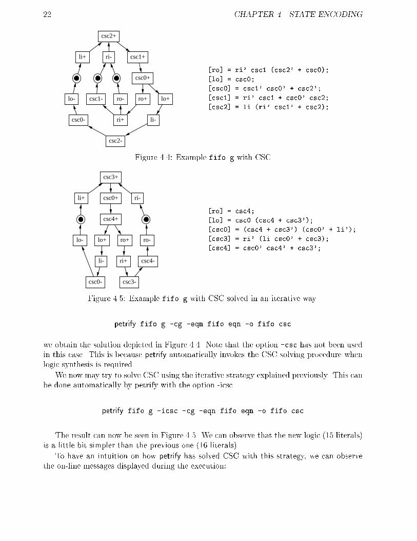
Figure �� Example fifo�g with CSC solved in an iterative way�

petrify fifo�g �cg �eqn fifo�eqn �o fifo�csc

we obtain the solution depicted in Figure �� Note that the option �csc has not been usedin this case� This is because petrify automatically invokes the CSC solving procedure whenlogic synthesis is required�

We now may try to solve CSC using the iterative strategy explained previously� This canbe done automatically by petrify with the option �icsc�

petrify fifo�g �icsc �cg �eqn fifo�eqn �o fifo�csc

The result can now be seen in Figure �� We can observe that the new logic �� literals�is a little bit simpler than the previous one �� literals��

To have an intuition on how petrify has solved CSC with this strategy� we can observethe on�line messages displayed during the execution�

�� PUTTING ALL THE ENGINES TO WORK ��

State coding conflicts for signal ro

State coding conflicts for signal lo

The STG has no CSC�

Adding state signal� csc�

State coding conflicts for signal lo

State coding conflicts for signal csc�






Adding state signal� csc

Removing signal csc� to improve CSC iteratively�


State coding conflicts for signal csc



Removing signal csc to improve CSC iteratively�





The STG has CSC�

�� Putting all the engines to work

As mentioned before� petrify can be tuned in di�erent ways to solve CSC� We now illustratehow to increase the exploration of the solution space by using two new options�

petrify fifo�g �icsc� �fr�� cg �eqn fifo�eqn �o fifo�csc

The result is shown in Figure �� The logic complexity is now �� literals�The reason why the options �icsc� �fr�� yield a better solution can be intuitively

explained�

�icsc�� In sevaral methods within the tool� the state space is explored in regions of states�These regions roughly correspond to �places� in Petri nets� i�e� a region is the setof states in which a place is marked� Petrify also calculates smaller blocks of statesas intersections of the regions� The greater the number of intersections calculatedbetween regions the smaller the number of states of the new generated blocks� Thesize of these blocks determines the granualrity at which petrify explores the space ofsolutions� The options �csc and �icsc can be specied with a natural number� e�g��csc� or �icsc� The default number is �� The higher the number is� the smallerthe granularity of the exploration� Indeed� the smaller the granularity is� the better


csc3+

csc1+li+ri-

lo+ csc2+

li- ro+

csc1-

lo-

ri+

ro-

csc3-

csc2-

�ro� � csc��

�lo� � csc��

�csc�� csc�� csc�� csc�� li��


�csc�� ri� �li csc�� csc��

Figure �� Example fifo�g with CSC solved with a wider exporation of the space ofsolutions�

the exploration is performed� although more computationally costly� In practice� itis useless to try granularities smaller than the ones produced by �csc�� The defaultvalue often yields similar solutions�

�fr�� The exploration of the partitions of the state space for state signal insertion is done ina similar way as many computer game programs play� Think about programs playingchess� The program analyzes a position and starts calculating all possible combinationsstarting from the current position� thus generating a search tree� At each level of thistree� the program heuristically selects a subset of promising solutions that will be theseeds for the next level of the tree� This subset of solutions selected at each level iswhat petrify calls the �frontier� of solutions� The option �fr denes the size of thisfrontier� Indeed� the wider the frontier� the larger the set of solutions explored at theexpense of computational cost� If you are not in a hurry in nding a solution andthe problem to solve is not too large� you might even try the option �fr�� If notspecied� petrify works as follows� in the rst levels of the tree the frontier is around� � but decreases at each iteration until it reaches the minimum value of �� When �frnis specied� the value of the frontier remains constant during the exploration�

�� When CSC cannot be solved

Unfortunately� petrify cannot guarantee a solution to the state encoding problem even if itexists� Whenever that occurs� the designer must take some action in order to nd a solutionor make the task easier for petrify� Here are some suggestions�

� Try to make the exploration of the solution space more aggressive by using the options�cscn and �frw� as explained in the previous section�

� Change the specication� A possibility here is to use the option �er �see section ��to split events with disconnected excitation regions�

�� IRREDUCIBLE CSC CONFLICTS �

� Dene some inputs events as �slow� events to increase the chances of nding places toinsert state signals �see section �� for more details��

� Make timing assumptions �see chapter ��

However� there are con�icts for which no solution exists unless the specication is changedor timing assuptions are made in such a way that a non�speed�independent circuit can bederived� These are known as irreducible con�icts� Next section will discuss how to solvethem�

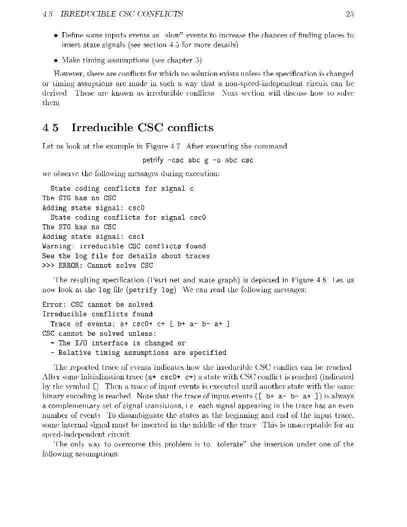
�� Irreducible CSC con�icts

Let us look at the example in Figure �� After executing the command

petrify �csc abc�g �o abc�csc

we observe the following messages during execution�

State coding conflicts for signal c






Warning� irreducible CSC conflicts found�

See the log file for details about traces�

�� ERROR� Cannot solve CSC�

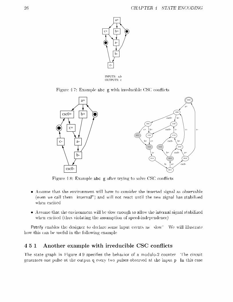
The resulting specication �Petri net and state graph� is depicted in Figure �� Let usnow look at the log le �petrify�log�� We can read the following messages�

Error� CSC cannot be solved�

Irreducible conflicts found�

Trace of events� a� csc�� c� � b� a� b� a� �

CSC cannot be solved unless�

� The I�O interface is changed or

� Relative timing assumptions are specified

The reported trace of events indicates how the irreducible CSC con�ict can be reached�After some initialization trace �a� csc�� c�� a state with CSC con�ict is reached �indicatedby the symbol �� Then a trace of input events is executed until another state with the samebinary encoding is reached� Note that the trace of input events �� b� a� b� a� �� is alwaysa complementary set of signal transitions� i�e� each signal appearing in the trace has an evennumber of events� To disambiguate the states at the beginning and end of the input trace�some internal signal must be inserted in the middle of the trace� This is unacceptable for anspeed�independent circuit�

The only way to overcome this problem is to �tolerate� the insertion under one of thefollowing assumptions�


INPUTS: a,bOUTPUTS: c

a+

b+c+

a-

b-

c-

Figure �� Example abc�g with irreducible CSC con�icts�

a+

csc0+ b+

c+

a-

b-

c-

csc0-

0000

1000

a+

1100

b+

1001

csc0+

1101

csc0+b+

1011

c+

1110

c-

1111

c+b+

1111

csc0-

0111

a-

1010

c-

b+

0011

b-

1011

b+ csc0-

0010

c-

a+

a+ csc0-

Figure �� Example abc�g after trying to solve CSC con�icts�

� Assume that the environment will have to consider the inserted signal as observable�even we call them �internal�� and will not react until the new signal has stabilizedwhen excited�

� Assume that the environment will be slow enough to allow the internal signal stabilizedwhen excited �thus violating the assumption of speed�independence��

Petrify enables the designer to declare some input events as �slow�� We will illustratehow this can be useful in the following example�

�� Another example with irreducible CSC con�icts

The state graph in Figure �� species the behavior of a modulo�� counter� The circuitgenerates one pulse at the output q every two pulses observed at the input p� In this case

�� TIMING CONSTRAINTS IMPOSED BY INTERNAL ACTIVITY ��

INPUTS: pOUTPUTS: q

00

10

p+

01

q-

00

p-

00

q+

10

p+ p-

�inputs p

�outputs q

�state graph

s� p� s� p� s� p� s� p� s� q� s� q� s�

�marking �s��

�slowenv

�end

Figure �� Example counter�g with irreducible CSC con�icts and slow events�

p+ csc2+

q-csc0-

p- csc1+

csc1- csc2-

p+ csc0+

q+ p-

�q� � p� csc��

�csc�� p� csc�� csc��

�csc�� csc� �p� � csc��

�csc�� q� csc� � p�

Figure �� Solution for counter�g�

the format to describe state graphs in petrify has been used�This specication has irreducible CSC con�icts� If we start fom the initial state and after

ring the trace p� p� p� p� we reached another state with the same encoding as the initialstate� but with di�erent behavior for the output signal q�

However� we can assume that the pulses produced by the environment are wide enoughthat any internal activity inside the circuit will be allowed to stabilize� This can be indicatedby the statement �slowenv that indicates that all events of the input signals are slow�In the case that assumption should be made for only a subset of the input events� thestatement �slow can be used� e�g� �slow p�� When the astg format is used to specifySTGs� the �slow statement can be followed by individual instances of signal transitions� e�g��slow a�� a�� b� c��

Let us now solve CSC and derive logic equations�

petrify counter�g �cg �eqn counter�eqn �o counter�csc

The obtained solution is depicted in Figure ��

�� Timing constraints imposed by internal activity

If we look at the solution presented in Figure �� we can observe that some of the in�put events are �delayed� by non�observable internal events� Obviously� this violates the


input�output interface initially specied for the circuit� However� we have also seen thatthis violations are tolerated under some timing assumptions�

Whenever some of these timing assumptions are efectively used to make some transfor�mations of the state space� petrify gives some warning messages in the log le� The rstpart of petrify�log after having solved CSC is the following�

Number of added state signals � �

��

� Paths of internal events delaying input events� �

��

csc� �� p��

csc�� p��

csc�� p��

The information concerning �delaying input events� indicates that the new specicationinvolves some internal activity that must be allowed to stabilize before new input eventsoccur� As an example� the rst message indicates that event csc� is �in progress� whenp�� is already enabled� For a safe functioning of the circuit� csc� should occur beforep�� occurs� These are timing assumptions that should be formally veried or validatedwithin the actual environment in which the circuit is embedded�

The second section of the le concerns �Output � Input Delays��

��

� Input �� Input Delays� �

��

Average delay � �� events

Worst�case delay � �� events

Input events with worst�case delay� p�

� Input events preceding p�� p��




This is an attempt to provide information about response time of the circuit� It roughlyestimates the number of non�input events that must be red before an input event is enabled�In the solution shown in Figure �� we can observe that there is one input event with venon�input transitions preceding it�

�q�� csc�� csc�� csc � � q�� p�

This is the critical response time of the circuit� In all other cases� the circuit only res oneevent before enabling some input event of the environment� In average� the response time is�� events�

Chapter �

Synthesis with relative timing

assumptions

The synthesis of speed�independent circuits assumes a delay model that can be consideredtoo conservative for the temporal behavior we may expect from the actual environment ofthe circuit and the technology used to implement it�

By making some timing assumptions on the behavior of the environment and the circuititself� the logic complexity of the circuit can be simplied� However� the property of speed�independence may be lost� i�e� the circuit may not react correctly for any delay of thecomponents of the system� For this reason� it is crucial to know under which conditions thecircuit behaves properly�

Petrify incorporates synthesis methods for hazard�free circuits under timing assumptions�It also provides backannotation that indicates the required timing constraints for a properfunctioning of the circuit�

�� Timing assumptions

In this section� the timing assumptions that petrify can �understand� will be discussed� Allof them are relative timing assumptions which means that they refer to the specic orderingof events with regard to other events� In contrast� absolute timing assumptions are speciedin terms of time intervals for the occurrence or enabling of events�

The di�erence between relative and absolute timing assumptions is illustrated in Fig�ure �� The gure depicts a part of a Petri net �arcs implicitly represet ��input ��outputplaces that can hold tokens�� Assume that the designer knows the execution delays forsome of the events and these delays can be expressed as time intervals� e�g� ��b� � �� c� � �� d� � �� and ��e� � �� The delays for events a and x are unknown�

Under the previous assumptions� it can be deduce that b will always occur before e� butno assumption can be made about the ordering of events c and d� since the enabling timeof event c is also determined by the ring time of event x� These analysis would roughlycorrespond to the analysis done when absolute timing assumptions are used�

With relative timing assumptions the designer can direcly indicate that b will occur beforee and that c will occur before d� Indeed� it is the designer�s responsability to ensure that

��

� CHAPTER �� SYNTHESIS WITH RELATIVE TIMING ASSUMPTIONS

b

x

d

a

c

e

x

(a) (b)

b

d

a

c

e

Figure �� Relative and absolute timing assumptions�

those assumptions hold� The fact that c will occur before d can be deduced by the designerif it is known� for example� that x will always occur before a�

Three di�erent types of relative timing assumptions can be specied in petrify�

� Firing order of concurrent events

� Simultaneous occurrence of concurrent events

� Early enabling

To properly understand the semantics of relative timing constraints� the concepts ofenabling region and �ring region must be introduced� Given a state graph� the enablingregion of event a� EN�a� is dened as the set of states in which a is enabled� The �ringregion of event a� FR�a�� is dened as the set of states in which a is allowed to re�

Whereas in speed�independent circuits� both concepts are the same �an event can re assoon as it is enabled�� they substantially di�er when timing assumptions are considered� Anevent can be enabled at some state but cannot re until the system reaches its ring region�

All these timing assumptions are specied in the input le where the STG is described�They should go after the graph �or state graph� specication and before the �end statement�

�� Firing order of concurrent events

This timing assumption is specied with the following syntax�

�time a � j b

The meaning of that statement is the following�

Whenever events a and b are concurrent �i�e� simultaneously enabled and not incon�ict�� a will always �re before b

To illustrate how the assumption is made by petrify we will use the example of Figure ��We can observe that events a and b have di�erent relations� They can be concurrent

�both enabled in state s�� or ordered �a is enabled in s� and b is enabled in s�� The timingassumption only applies to those states in which the events are concurrent�

�� TIMING ASSUMPTIONS ��

c

a

d

e b

s0

s6

a

s1

b

s3

b a

s4

e

s2

c

s7

b

s5

a

d

Figure �� Illustration of timing assumptions on event ordering�

The application of the timing assumption would mean that b will not re in s�� As aconsequence� state s� will become unreachable in the timed domain�

With regard to event b� petrify also considers that s� is a �don�t care� state for theenabledness of event b� i�e� after logic synthesis two di�erent solutions could be reported�

� One in which b is enabled in s�� Still� the timing assumptions will make s� unreachable�thus b will not re until s� is reached�

� One in which b is not enabled in s�� In this way� the ordering a � b will be forcedby the logic of the circuit� i�e� no timing assumption is required for this solution to bevalid�

This can be formally expressed as follows�

fs�g � FR�b� � EN�b� � fs�� s�g

Petrify will choose a solution for EN�b� that minimizes the cost of the logic�

�� Simultaneous occurrence of concurrent events

This timing assumption is specied with the following syntax�

�time a�b�c

An example of this assumption is shown in Figure �� The meaning of the simultaneitytiming assumption is the following�

Let us take the states in which a and b are enabled and concurrent� Event c willnot �re in any of the successor states until a and b have �red� This assumptiononly applies when c is triggered by either a or b or both�

�� CHAPTER �� SYNTHESIS WITH RELATIVE TIMING ASSUMPTIONS

x

a b

c

s0

s2

x

s6

a

s1

b

s5

c

s4

b a

s3

b c

Figure �� Simultaneity timing assumptions

Informally� the assumptions describes the situation in which the ring time di�erence betweena and b is not distinguishable by event c� Looking a the example� this would mean that thesystem would produce the same observable behavior if c would be �triggered� by b or byboth events a and b�

Looking at the state graph of Figure �� the simultaneity constraint indicates that cwould not re in state s� and� therefore� state s� would become unreachable� On the otherhand� event c would be allowed to be enabled in the states s�� s� and s�� Thus�

fs�g � FR�c� � EN�c� � fs�� s�� s�g

The simultaneity timing assumptions can be extended to larger number of events asfollows�

�time a�b�c�d�x y z

meaning that the ring time of events a� b� c and d is considered to be non�distinguishablewith respect to events x� y and z�

�� Early enabling

This timing assumption will be illustrated by the example in Figure ��Early enabling assumptions are specied with the following syntax�

�time c�b

The formal meaning of this assumption is the following�

Let us take all those states s � i in which c is not enabled� but becomes enabledafter �ring b �i�e� b triggers c�� Then� the states si can potentially belong toEN�c��

�� THE XY Z EXAMPLE ��

x

a d

b

c

s0

s2

x

s4

a

s1

d

s8

b

s3

d a

s6

d

s7

c b

s5

cd

Figure �� Example to illustrate early enabling assumptions�

Informally� this assumptions indicates that event c can be enabled before it must re�However� the delay of the logic implementing c will ensure that c will re after b� Indeed�this may be seen as a risky assumption� since the logic of signals b and c are not knownbefore logic synthesis� Relative timing assumptions require a post�verication than ensuretheir validity� In the case they do not hold� some actions must be taken� for example�

� Resynthesize the circuit without those invalid assumptions or

� Change the delays of the components of the circuit �e�g� by transistor sizing or delaypadding� so that the assumptions become valid�

In the previous example� EN�c� and FR�c� are dened as follows�

fs�� sg � FR�c� � EN�c� � fs� s�� s�� sg

The early enabling assumptions can be extended to chains of events� In the previousexample� the following assumptions could be also specied�

c�b�a

indicating that EN�c� can be extended up to the enabling of event a� However� no assumptionis made about the enabledness of b with regard to a�

�� The xyz example

Let us illustrate the usage of timing assumptions in the well�known xyz example shown inFigure ��


x+

y+ z+

z-

x- y-

000

100

x+

110

y+

101

z+

010

y-

111

z+ y+

001

x-

011

z-

x- y+

Figure �� The xyz example�

A speed�independent implementation of the behavior with complex gates would be thefollowing�

�x� � z� �x � y��

�y� � z � x�

�z� � y� z � x�

Let us assume that x� y and z are output signals and we conjecture that the ring ofy� will occur always before the ring of x�� We can intuitively deduce this by observingthat y� is always enabled before x� and that the logic for signal x in the speed�independentimplementation looks more complex than the logic for signal y�

We can then add some timing assumption to our specication�

�outputs x y z

�graph

x� y� z�

z� x�

y� z�

x� z�

z� y�

y� x�

�marking ��y� x��

�time y��x�

�end

and then synthesize a circuit with the following command�

petrify xyz�g �cg �topt �eqn xyz�eqn �no

The option �topt indicates that petrify must take timing assumptions into considerationto derive logic� The following logic is obtained�

�x� � z� �x � y��

�y� � z � x�

�z� � x�

�� THE XY Z EXAMPLE �

in which we observe a drastic simplication of the logic for signal z� Petrify has takenadvantage of the timing assumption to consider the state � as unreachable and implementz simply as a bu�er�

But as important as the solution is the feedback that petrify reports about the timingassumptions used for each solution� If we look at the le petrify�log� we can analyzedi�erent solutions for each signal� In particular� among the solutions reported for signal z�we have the following�

z � x

� triggers�SET�� x� �� z�

� triggers�RESET�� x� �� z�

� � transistors � n p�

� Estimated delay� rising � �� falling � ��

� Timing assumptions �concurrency�� y��x�

�� other solutions ��

z � y� z � x


� triggers�RESET�� y� x�� z�

� �� transistors �� n � p�


� Speed independent �no timing assumptions�

The rst solution corresponds to the one obtained with timing assumptions� The sec�ond one corresponds to the speed�independent implementation� There are two importantinformations reported for the solutions�

Timing assumptions Petrify indicates that the solution z�x is only valid under the as�sumption that y� res before x�� The solution z � y� z � x is valid under anytiming asumption �speed�independent solution�� The timing assumptions reported bypetrify are not necessarily the same as the one dened in the specication� Petrify

always tries to report the less stringent assumptions that make the solution valid�

Trigger signals For each solution petrify also indicates which events are triggered the risingand falling transitions of the signal� Note the di�erence for the trigger events of z��In the �timed� solution� y� is no longer triggering z� since it is assumed to re beforex�� This information is much more relevant when �early enabling� assumptions aredone for synthesis�

Let us now try another type of timing assumption� We can also observe that y� and z�are enabled simultaneously� If the delays of their gates would be similar� we could considerthat the ring time of y� and z� would not be distinguishable with respect to event x��The specication now would be as follows�


�outputs x y z

�graph

x� y� z�

z� x�

y� z�

x� z�

z� y�

y� x�

�marking ��y� x��

�time y��z� � x�

�end

After executing the same command as above� the following solution is obtained�

�x� � y��

�y� � z � x�

�z� � x�

This is a signicant improvement � but � � � under which assumptions is this solution correct Again� the le petrify�log will give us relevant information about that� Let us rst lookat di�erent solutions for x and compare with the speed�independent solution�

x � y�

� triggers�SET�� y� �� x�

� triggers�RESET�� y� �� x�



� Concurrency reduction� y��x�

� Timing assumptions �early enabling�� z��x�

x � y� z�


� triggers�RESET�� y� z�� x�




�� other solutions ��

x � z� �x � y��


� triggers�RESET�� z� �� x�




�� AUTOMATIC DERIVATION OF TIMING ASSUMPTIONS ��

The solution x � y� is generated by disabling x� in state � � �where it was initiallyenabled�� This makes the state � unreachable� But note that� in this case� it is notunreachable due to timing assumptions� but due to the fact that the logic for x does notenable x� in state � �� This is what the message


means� In other words� the fact that y� res before x� res does not need to be veried bymaking timing assumptions� It is something that the logic of the circuit already guarantees�

Still there is another inmportant assumption for that solution�


This indicates that x� is enabled in such a way that it becomes concurrent with z��now x� is also enabled in state �� The assumption for correctness is that z� shouldre before x�� To verify that assumption at circuit level� one might need some additionalinformation� how much early is x� enabled Again� this information is provided in thesection of trigger signals� We may realize that now it is y� that triggers x� �it was z� inthe speed�independent solution�� Thus� by combining these informations we can determinewhen the enabling of an event is started �trigger events� and the event is allowed to re�when other concurrent events have already red�� Now� it is time for the designer to decidewhether these assumptions are realistic or can be met by the implementation�

Still� there is another interesting solutions that appears in the le petrify�log� x � y�

z�� This solution makes the state � again reachable� since x� is enabled in state � �� Butx� is also enabled earlier in state �� and the assumption z��x� must still be ensured�

An important aspect of the information provided by petrify is that di�erent timing as�sumptions must be ensured for each di�erent solution of each signal� The selection of onesolution for one signal does not a�ect the assumptions made for other gates� However� thecombination of all the solutions for each gate may lead to a set of simpler constraints� Cur�rently� it is the designer who has to gure out how these constraints interact among them�What petrify guarantees is that the solutions will be valid if the timing assumptions reportedfor each individual solution of each signal are met�

�� Automatic derivation of timing assumptions

Bearing in mind that the designer tipically likes to improve the performance of the cir�cuits and that some assumptions are easily derivable by just looking at the structure of thespecication� petrify has also made an e�ort to automatically generate �reasonable� timingassumptions�

With this strategy� petrify only wants to simplify the job of the designer� but not tosusbtitute it� Indeed� petrify will nally report which assumptions have been generatedautomatically and which of them are actually used for each solution� It is then the designer�sIndeed� petrify will nally report which assumptions have been generated automatically andwhich of them are actually used for each solution� It is then the designer�s responsability toguarantee tha validity of the timing assumptions�


�� Delay model for the automatic derivation of timing assump�

tions

The following model is considered for the delay of a signal transition �delay from its enablingtime to its ring time��

Non�input signals� each gate implementing a non�input signal has a delay in the interval�� where � � �� Thus� the delay of two gates is always greater than thedelay of one gate�

Input signals� have a delay in the interval �� Thus� the delay of the environmentis always greater than the delay of one gate�

Slow input signals� have a delay in the interval �k�� where k any arbitrarily large con�stant� The delay k indicates that the enabling of a slow input signal transition alwaysallows the completion of any internal activity in the circuit �ring of enabled non�inputsignals��

Delay padding� the delay of any gate implementing any non�input signal can be lengthenedafter logic synthesis� e�g� by transistor sizing or delay padding� to meet the requiredtiming assumptions�

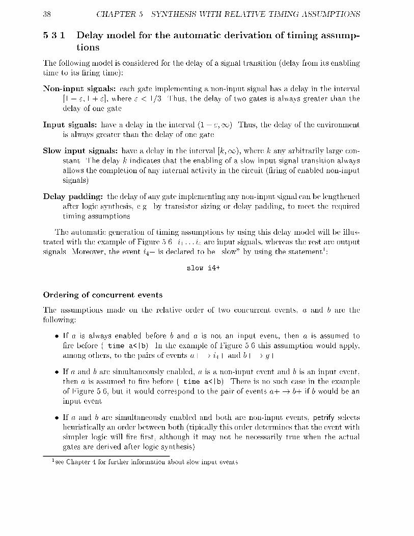
The automatic generation of timing assumptions by using this delay model will be illus�trated with the example of Figure �� i� � � � i� are input signals� whereas the rest are outputsignals� Moreover� the event i�� is declared to be �slow� by using the statement��

�slow i��

Ordering of concurrent events

The assumptions made on the relative order of two concurrent events� a and b are thefollowing�

� If a is always enabled before b and a is not an input event� then a is assumed tore before ��time a��b�� In the example of Figure �� this assumption would apply�among others� to the pairs of events a�� i�� and b�� g��

� If a and b are simultaneously enabled� a is a non�input event and b is an input event�then a is assumed to re before ��time a��b�� There is no such case in the exampleof Figure �� but it would correspond to the pair of events a�� b� if b would be aninput event�

� If a and b are simultaneously enabled and both are non�input events� petrify selectsheuristically an order between both �tipically this order determines that the event withsimpler logic will re rst� although it may not be necessarily true when the actualgates are derived after logic synthesis��

�see Chapter � for further information about slow input events

�� AUTOMATIC DERIVATION OF TIMING ASSUMPTIONS ��

i1+ i2+

a+ b+ c+ r+ s+

i3+ i4+ f+

h+

d+ e+ g+

Figure �� Example for automatic generation of timing assumptions�

� No assumptions are done for pairs of events that can be enabled in di�erent order inthe untimed domain� For example� for events i�� and f� we can nd event tracesin which i�� is rst enabled �e�g� i�� b�� c�� and in which f� is rst enabled �e�g�i�� c�� b��

Simultaneous trigger events

In case two non�input events� a and b� are enabled simultaneously and another event c istriggered by a or b �or both�� a simultaneity assumption is automatically generated �a�b�c��

Unfortunately� petrify only makes this analysis for pairs of simultaneous events� Assump�tions on more than two simultaneous events are left to be specied by the designer�

There are several examples of simultaneity assumptions in Figure �� b��c��f�� r��s��h��etc�

Early enabling

When several non�input events have a trigger relation among them� petrify automaticallygenerates early enabling assumptions� taking into account that the delays of the gates canbe properly lengthened to meet the ordering relations of the specicatin�

In the example of Figure �� there are chains of events that have a trigger relation amongthem� c� � f� � g�� h� and r� � h�� The following assumptions are automaticallygenerated�

�time f� � c�

�time g� � f� � c�

�time h� � g� � f� � c�

�time h� � r�

� CHAPTER �� SYNTHESIS WITH RELATIVE TIMING ASSUMPTIONS

Ordering of slow input events� a generalization of the fundamental mode as�

sumption

Under the assumption that the delay of slow input events is long enough to enable thecircuit stabilize when other internal activity is in process� petrify can automatically generateassumptions on the ring order of slow events�

The timing analysis is performed in such a way that only concurrent non�input eventswith a common predecessor history with the slow input event are assumed to re rst� Thisintuitive idea will be more clear after looking at the example in which i�� is the only slowinput event�

Events i�� and g� have a common predecessor event in their history� i�� Moreover�no other input events precede the enabledness of i�� and g� since the ring of i�� Ifwe consider the ring time of i�� as the starting point for timing analysis �t � �� andconsidering the delay model for automatic assumptions� g� will re in the interval �� i�e� three gate delays� On the other hand� the ring interval for i�� will be inthe interval �k � � � �� where k can be arbitrarily large� Therefore� petrify will deducethat the ring time of g� will be always before the one for i��

Note that this assumption does not hold when the considered event is h�� since nocommon preceding history with i�� can be found with no other input events enabled inbetween� For a similar reason� no ordering assumption can be made for the ring of i�� andd� since an input event �i�� precedes d� before meeting the common preceding point inwhich timing analysis can start�

Technically� this common point in the history of two events is called local nodal point� Theanalysis based on local nodal points generalizes the concept of fundamental node typicallyused for the synthesis of burstmode specications� Burst�mode machines work under theassumption that each state of the specication is a global nodal point� i�e� no non�inputactivity is enabled in the state� From the point of view of specication� fundamental modedoes not allow any concurrency between the environment and the circuit�

The notion of slow input event takes the advantages of fundamental mode assumptions�logic can be simplied� and speed�independent assumptions �concurrency is not sacrized��As an example� the denition of slow input events would allow to synthesize a system withseveral sets of handshake signals by assuming a �local� fundamental mode operation witheach individual handshake� but maintaining the concurrency among di�erent independentsets of handshakes� One of these examples is the VME bus controller described in Chapter ��

Finally� all the automatically generated assumptions for the example of Figure �� arethe following�

�time b��a�

�time c��a�

�time a��i��

�time a��e�

�time a��f�

�time a��g�

�time a��h�

�time c��b�

�� THE XY Z EXAMPLE REVISITED ��

�time b��i��

�time b��d�

�time b��f�

�time b��g�

�time b��h�

�time c��i��

�time c��d�


�time c��e�

�time s��h�

�time s��r�

�time a��i��


�time f��i��

�time g��i��

�time f��c�

�time g��f��c�

�time h��g��f��c�

�time h��r�

�time a��c��f�

�time b��c��f�

�time r��s��h�

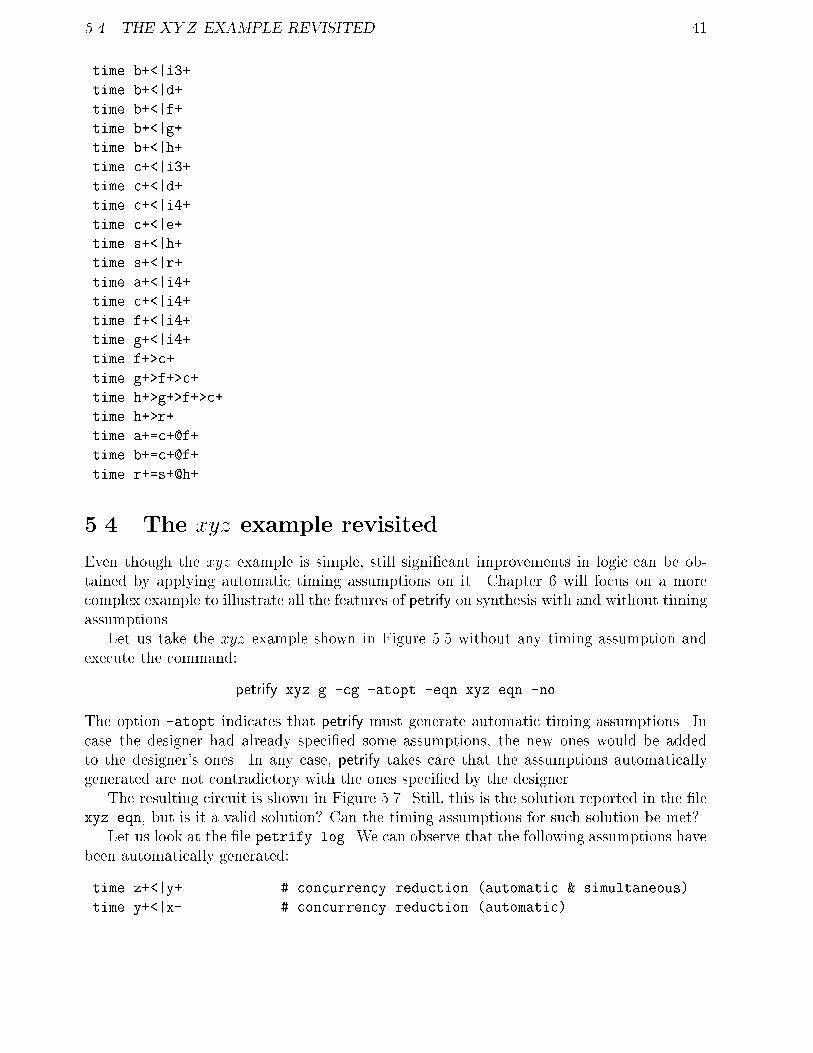
�� The xyz example revisited

Even though the xyz example is simple� still signicant improvements in logic can be ob�tained by applying automatic timing assumptions on it� Chapter � will focus on a morecomplex example to illustrate all the features of petrify on synthesis with and without timingassumptions�

Let us take the xyz example shown in Figure � without any timing assumption andexecute the command�

petrify xyz�g �cg �atopt �eqn xyz�eqn �no

The option �atopt indicates that petrify must generate automatic timing assumptions� Incase the designer had already specied some assumptions� the new ones would be addedto the designer�s ones� In any case� petrify takes care that the assumptions automaticallygenerated are not contradictory with the ones specied by the designer�

The resulting circuit is shown in Figure �� Still� this is the solution reported in the lexyz�eqn� but is it a valid solution Can the timing assumptions for such solution be met

Let us look at the le petrify�log� We can observe that the following assumptions havebeen automatically generated�

�time z��y� � concurrency reduction �automatic simultaneous�

�time y��x� � concurrency reduction �automatic�


yx z

Figure �� Optimized circuit for the xyz example�

�time x��y��z��y� � early enabling �automatic�

�time x��y��z� � early enabling �automatic�

�time x��z� � early enabling �automatic�

�time z��y� � early enabling �automatic�

�time z��x� � early enabling �automatic�

�time y��z� � early enabling �automatic�

�time y��z��x��z� � early enabling �automatic�

�time y��z��x� � simultaneity �automatic�

and the following information is reported for the solutions�

x � y�


� triggers�RESET�� y� �� x�




� Timing assumptions �concurrency�� z��y�

��

y � z

� triggers�SET�� z� �� y�

� triggers�RESET�� z� �� y�



� Concurrency reduction� z��y�


��

z � x


� triggers�RESET�� x� �� z�



� Timing assumptions �concurrency�� y��x�

The provided timing information can be summarized as follows�

�� THE XY Z EXAMPLE REVISITED ��

� The ring order z�� y� is required for the solution x � y� to be valid� but the ringorder z� � y� is enforced by the solution y � z that reduces concurrency and makesthe state �� unreachable�

� The ring order y�� x� is required for the solution z � x to be valid� but the ringorder y�� x� is enforced by the solution x � y� that reduces concurrency and makesthe state � unreachable�

Therefore� the enforced concurrency reduction ensures the validity of the timing assump�tions and a speed�independent circuit is obtained � This is an example on how concurrencyreduction does not always imply a loss of performance� The reduction on logic results in amore e�cient circuit�


Chapter �

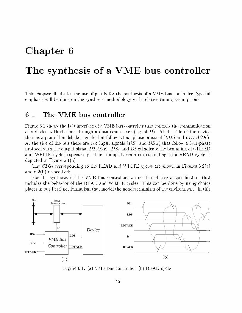
The synthesis of a VME bus controller

This chapter illustrates the use of petrify for the synthesis of a VME bus controller� Specialemphasis will be done on the synthesis methodology with relative timing assumptions�

�� The VME bus controller

Figure �� shows the I�O interface of a VME bus controller that controls the communicationof a device with the bus through a data transceiver �signal D�� At the side of the devicethere is a pair of handshake signals that follow a four�phase protocol �LDS and LDTACK��At the side of the bus there are two input signals �DSr and DSw� that follow a four�phaseprotocol with the output signal DTACK� DSr and DSw indicate the beginning of a READand WRITE cycle respectively� The timing diagram corresponding to a READ cycle isdepicted in Figure ��b��

The STGs corresponding to the READ and WRITE cycles are shown in Figures ��a�and ��b� respectively�

For the synthesis of the VME bus controller� we need to derive a specication thatincludes the behavior of the READ and WRITE cycles� This can be done by using choiceplaces in our Petri net formalism that model the nondeterminism of the environment� In this

DSr

DSw

DTACK

LDS

LDTACK

Device

VME Bus

Controller

D

TransceiverDataBus

�a�

DSr

LDS

LDTACK

D

DTACK

�b�

Figure �� a� VME bus controller� �b� READ cycle�

�

�� CHAPTER �� THE SYNTHESIS OF A VME BUS CONTROLLER


lds+

ldtack+ dsr+

d+

dtack+

ldtack-

dsr-

dtack-lds-

d-

�a�

INPUTS: dsw,ldtackOUTPUTS: dtack,lds,d

lds+

ldtack+ d+

d- dsw+

dtack+

ldtack-

dsw-

lds-

dtack-

�b�

Figure �� STGs for the �a� READ and �b� WRITE cycles�

case� the nondeterminism comes from the fact that the environment can choose to initiate aREAD or a WRITE cycle after the completion of the previous cycle�

An STG describing the complete behavior of the controller is shown in Figure ��a��We can observe that some signal transitions� e�g� lds� have multiple instances in the STG�The indices � and have been used to distinguish events in the READ and WRITE cyclesrespectively�

There is also the possibility of representing the whole behavior in an STG with onlyone transition for each di�erent label� The STG can be obtained by petrify by using thecommand�

petrify vme�g �o vme��label

The result is shown in Figure ��b�� However� this representation is much less readablethat the previous one� For this reason we will use the STG of Figure ��a� to synthesizethe circuits presented in this chapter� With that representation� the specication of timingassumptions will become much more intuitive� since we will be able to independently denethem for the READ and WRITE cycles�

�� Speedindependent implementation

Let us rst derive a speed�independent implementation of the VME bus controller� Thenotation used for the representation of generalized C elements is shown in Figure ��

After executing the command

petrify vme�g �gc �fr�� eqn vme�eqn �log vme�log �o vme�csc

The option �fr�� increases the width of the exploration when solving CSC con�icts� Thesolution obtained is depicted in Figure �� One internal signal� csc � has been inserted toencode the states�

�� SPEED�INDEPENDENT IMPLEMENTATION ��

ldtack-

lds-

dsr+

lds+/1

ldtack+/1

d+/1

dtack+1

dsr-

d-/1

dsw+

d+/2

lds+/2

ldtack+/2

d-/2

dtack+/2

dsw-

dtack-

Read cycle Write cycle

�a�

INPUTS: dsr,dsw,ldtackOUTPUTS: dtack,lds,d

dsr-

dtack-dsw-

dtack+

d-

lds-

ldtack-

dsr+ dsw+

lds+ d+

ldtack+

�b�

Figure �� a� STG for the VME bus controller� �b� Equivalent STG with only one transitionfor each signal event�

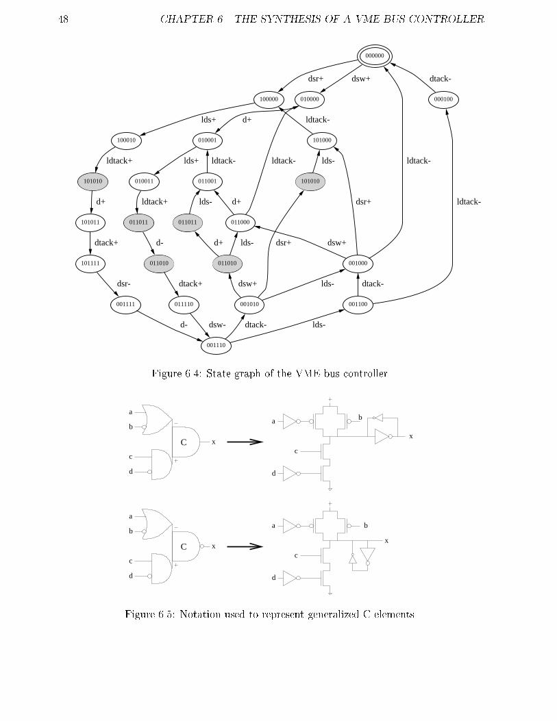
�� CHAPTER �� THE SYNTHESIS OF A VME BUS CONTROLLER

000000

010000

dsw+

100000

dsr+

000100

dtack-

010001

d+

100010

lds+

101000

ldtack-

010011

lds+

101010

ldtack+

011001

ldtack-

101010

lds-

011011

ldtack+

101011

d+

011000

ldtack-

d+

011010

d-

101111

dtack+

011011

lds-

011110

dtack+

011010

lds-d+

001000

ldtack-

dsr+

dsw+

001111

dsr-

001110

dsw-

001010

dsr+

dsw+ lds-

001100

ldtack-

dtack-

d- dtack- lds-

Figure �� State graph of the VME bus controller�

C

C x

a

b

c

d

a b

c

d

x

c

d

b

a

x

a

c

d

x

b

Figure �� Notation used to represent generalized C elements�

�� SPEED�INDEPENDENT IMPLEMENTATION ��

p3

csc0+

p2

lds+/1

lds+/2

ldtack+/1

ldtack-

dsr+

d+/1

lds-

dtack+/1

dsr-

d-/1

p1

csc0-dsw-

dtack-

p0

dtack+/2

dsw+

d-/2

d+/2

ldtack+/2

C

C

C

csc0

csc0

d

csc0

csc0

csc0

csc0

csc0

ldtack

ldtack

ldtack

dsw

dsw

dsw

dsw

dtack

lds

dsr

dsr

dsr

dsr

d

d

d

d

Figure �� Specication �vme�csc� and speed�independent implementation of the VME buscontroller�

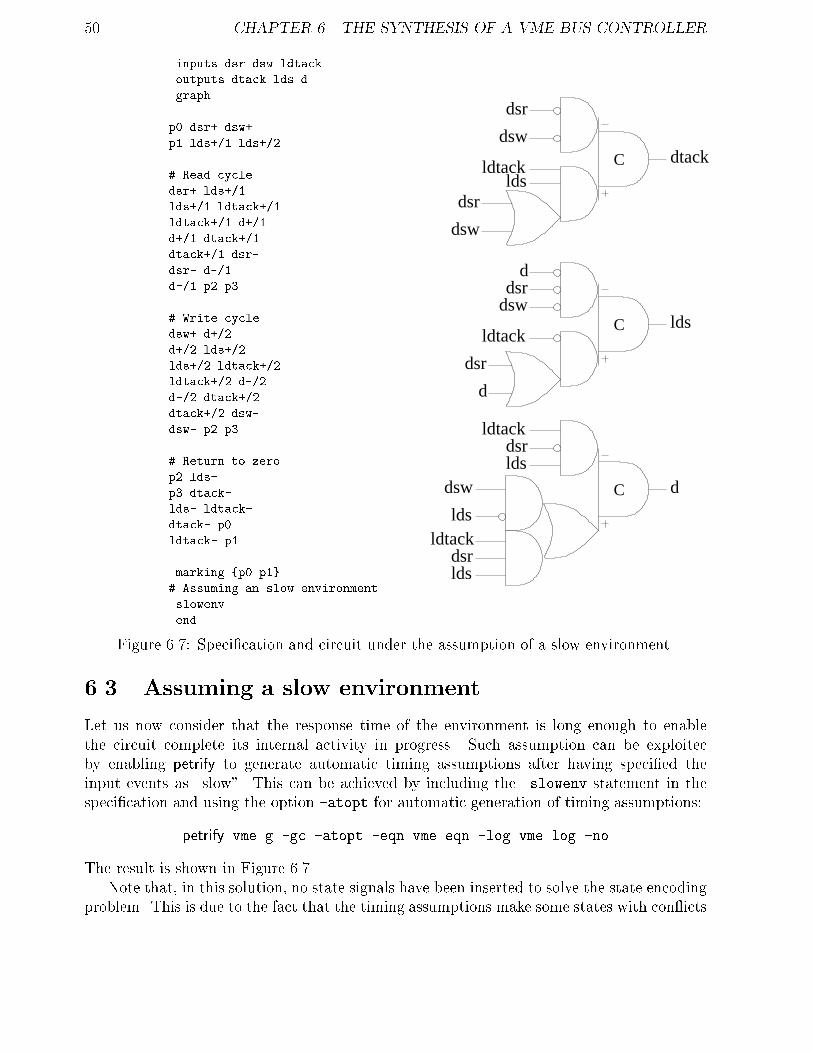
CHAPTER �� THE SYNTHESIS OF A VME BUS CONTROLLER

�inputs dsr dsw ldtack

�outputs dtack lds d

�graph

p� dsr� dsw�

p� lds�� lds��

� Read cycle

dsr� lds��

lds�� ldtack��

ldtack�� d��

d�� dtack��

dtack�� dsr�

dsr� d��

d�� p� p

� Write cycle

dsw� d��

d�� lds��

lds�� ldtack��

ldtack�� d��

d�� dtack��

dtack�� dsw�

dsw� p� p

� Return to zero

p� lds�

p dtack�

lds� ldtack�

dtack� p�

ldtack� p�

�marking p� p��

� Assuming an slow environment

�slowenv

�end

C

C

C

dtacklds

d

lds

dsr

dlds

ldtack

dswdsr

ldtack

dsw

dsw

lds

ldsdsr

ldtack

d

dsr

ldtack

dsr

dsw

dsr

Figure �� Specication and circuit under the assumption of a slow environment�

�� Assuming a slow environment

Let us now consider that the response time of the environment is long enough to enablethe circuit complete its internal activity in progress� Such assumption can be exploitecby enabling petrify to generate automatic timing assumptions after having specied theinput events as �slow�� This can be achieved by including the �slowenv statement in thespecication and using the option �atopt for automatic generation of timing assumptions�

petrify vme�g �gc �atopt �eqn vme�eqn �log vme�log �no

The result is shown in Figure ��Note that� in this solution� no state signals have been inserted to solve the state encoding

problem� This is due to the fact that the timing assumptions make some states with con�icts

�� ASSUMING A SLOW ENVIRONMENT �

unreachable� In this particular case� all con�icts dissapear�In order not to make the explanation too tedious� we will skip now the timing analysis

of the solution� but we will focus on the automatic timing assumptions generated by petrify�They are reported in the le vme�log�

�time lds��dsr� � concurrency reduction �automatic�

�time lds��dsw� � concurrency reduction �automatic�

�time lds��d�� concurrency reduction �automatic�

�time dtack��lds� � concurrency reduction �automatic simultaneous�

�time dtack��ldtack� � concurrency reduction �automatic�




�time lds��d�� early enabling �automatic�

�time dtack��d�� early enabling �automatic�


�time lds�d�� early enabling �automatic�

�time dtack�d�� early enabling �automatic�

Note that the fourth assumption ��time dtack��lds�� corresponds to the ordering oftwo output events that are enabled simultaneous� The message !!automatic simulatenous��

indicates two important things� �� that the assumption has been generated automaticallyand �� that both events are enabled simultaneously and petrify gave priority to one of themwhen deciding the ring order�

This is one of the cases where the intervention of the designer can be useful� What wouldbe the solution if we would not assume any ring order or another ring order �

The rst possibility can be exploring by adding the following timing assumption in thespecication� �time lds��dtack�� indicating no assumptions should be made on the ringorder of both events�

The second possibility can be explored by adding the following timing assumption in thespecication� �time lds��dtack�� Let us now execute the same command as above� Thenew reported timing assumptions in vme�log will be the following�

�time lds��dtack� � concurrency reduction �specification�



�time lds��d�� concurrency reduction �automatic�





�time lds��d�� early enabling �automatic�



�time lds�d�� early enabling �automatic�

�time dtack�d�� early enabling �automatic�

Note that the rst timing assumption ��time lds��dtack�� comes now from the !!specification��and precludes petrify to generate the assumption �time dtack��lds� that would contradict

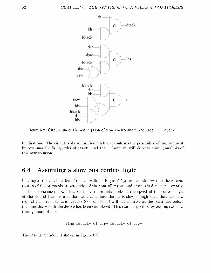
� CHAPTER �� THE SYNTHESIS OF A VME BUS CONTROLLER

C

C

C

ldsdsw

dsr

ldtack

dsr

dsw

ldtack

dsr

dlds

ldtack

dsw

lds

ldsdsr

dtack

ldtack

lds

lds

Figure �� Circuit under the assumption of slow environment and lds� �� dtack��

the rst one� The circuit is shown in Figure �� and conrms the possibility of improvementby reversing the ring order of dtack� and lds�� Again we will skip the timing analysis ofthis new solution�

�� Assuming a slow bus control logic

Looking at the specication of the controller in Figure ��a� we can observe that the return�to�zero of the protocols at both sides of the controller �bus and device� is done concurrently�

Let us consider now� that we know more details about the speed of the control logicat the side of the bus and that we can deduce that it is slow enough such that any newrequest for a read or write cycle �dsr� or dsw�� will never arrive at the controller beforethe handshake with the device has been completed� This can be specied by adding two newtiming assumptions�

�time ldtack� �� dsr� ldtack� �� dsw�

The resulting circuit is shown in Figure ��

�� TIMING ANALYSIS �

C

C

dtack

ldtack

lds

lds

dsr

dswlds

ddsr

ldtack

ldtack

dsr

dsw

ldtack

Figure �� Circuit under the assumption of a slow bus control logic�

�� Timing analysis

Let us now make the timing analysis of the nal solution depicted in Figure �� For this�we will rst study the information reported in the le vme�log about each gate�

SET�dtack�� lds�

RESET�dtack�� ldtack lds

�dtack� � dtack� �output inverter�

triggers�SET�� lds� � dtack�

triggers�RESET�� ldtack�� dtack�� ldtack�� dtack��


Estimated delay� rising � �� falling � ��

Concurrency reduction� lds��dtack�

Timing assumptions �early enabling�� d��dtack�� d��dtack��

��

lds� � dsw� dsr�

�lds� � lds� �output inverter�

triggers�SET�� dsr�dsw�� lds�

triggers�RESET�� dsr� � lds�� dsw� � lds��



Timing assumptions �concurrency�� ldtack��dsw� ldtack��dsr�

Timing assumptions �early enabling�� d��lds�� d��lds�


ldtack-

lds-

dsr+

lds+/1

ldtack+/1

d+/1

dtack+1

dsr-

d-/1

dsw+

d+/2

lds+/2

ldtack+/2

d-/2

dtack+/2

dsw-

dtack-

early enabling

firing order

concurrency reduction

Figure �� Timing assumptions for the nal solution of the VME bus�

��

SET�d�� dsr� ldtack

RESET�d�� dsw ldtack� � dsr ldtack

�d� � d� �output inverter�

triggers�SET�� dsr� � d�� ldtack�� d��

triggers�RESET�� ldtack�� d�� dsw�ldtack�� d��


Estimated delay� rising � �� falling � � ��

Concurrency reduction� ldtack��d��

Timing assumptions �concurrency�� ldtack��dsr�

The timing assumptions are represented and summarized in Figure �� We can distin�guish three types of timing arcs in that diagram�

Concurrency reduction arcs that denote the additional causality relations enforced by

�� TIMING ANALYSIS

C

C

d1

dtack

lds

ddsw

dsr

ldtack d2

Figure �� Delay padding to satisfy timing assumptions�

the logic �lds� � dtack� and ldtack� � d� �� These are not timing assumptionsthat must be veried for the circuit to be correct�

Firing order arcs that denote the assumed ring ordering of concurrent events for thecircuit to be correct� These are timing assumptions that must be veried or enforcedby delay padding�

Early enabling arcs that indicate the new trigger events for the early enabled events� Forexample� event lds� that is triggered by d � �� in the read cycle is now triggered bydsr�� This information is exrtacted by combining the early enabling timing assump�tions and the list of trigger events reported for each solution� These are assumptionsthat must be veried for the circuit to be correct� In the mentioned example� it mustbe veried that event d� �� will occur before event lds��

ldtack � � dsr� and ldtack � � dsw� were the assumptions that we made aboutthe speed of the bus control logic� Therefore� they can be considered as satised� However�the assumptions on early enabling of events must be carefully analyzed� since their validitydepends on the actual delays of the derived logic�

All the early enabling assumptions rely on the fact that the delay of gate d is shorterthan the delay of lds and dtack� Unfortunately� we see that gate d is more complex than theother gates� so these assumptions can be considered as unrealistic� Therefore� some changesmust be performed on the circuit to satisfy those assumptions�

A possible solution is depicted in Figure �� The delay d� should ensure that lds�� andlds� will re later than d�� and d�� respectively� even they are triggered simultaneously�The delay d� should ensure that dtack � �� and dtack � �� will re later than d � �� andd� �� respectively� Note that the chosen solution only delays the triggering e�ect of signalldtack� on dtack�� Another solution would have been to add a delay at the output of gatedtack� but this would also delay dtack�� which is not necessary for the correct functioning


of the circuit� Thus� we can see that the information reported by petrify allows to customizethe circuit such that timing assumptions are met for individual events of a signal� ratherthan for all the events of the signal�

Documents

Con - PUCRS - Portal