Computing the dispersion diagram and the forced response

of periodic elastic structures using a state-space formula-

tion

G. F. C. A. Assis1, E. J. P. Miranda Jr.2, D. Beli1, J. F. Camino1, J. M. C. Dos Santos1, J. R. F. Arruda1

1 University of Campinas - UNICAMP

Rua Mendeleyev, 200, CEP-13083-970, Campinas, SP, Brazil.

e-mail: arruda@fem.unicamp.br

2 Federal Institute of Maranhao - IFMA

Rua Afonso Pena, 174, 65010030, Sao Luıs, MA, Brazil.

AbstractIn the context of acoustic black hole investigations, recent works have proposed the use of a spatial state-

space formulation for one-dimensional elastic waveguides. The boundary value problem is thus transformed

into an initial value problem. Given that the state (displacements and forces) cannot be known a priori at any

given boundary, but the impedance can, the state-space problem is recast into an impedance formulation, in

the form of a Riccati equation. In this paper, this formulation is extended to compute the transfer matrix of a

periodic cell of a one-dimensional elastic waveguide. With this transfer matrix, not only can the dispersion

diagram be computed, but also the forced response of the finite structure. The simple case of an elastic rod

is used to illustrate the proposed method. The dispersion diagram is verified with the plane wave expansion

method, and the forced response is verified with the spectral element method. Numerical results show that

the proposed method is an efficient way to characterize wave propagation in period elastic structures.

1 Introduction

Linear elastodynamic problems are usually formulated as boundary value problems, which may be solved

analytically or numerically [1]. Analytical solutions are often derived in the frequency domain, which can be

referred to as spectral solutions. For simple structures, it is straightforward to derive solutions in the form of

finite elements in the frequency domain. This semi analytical approach is known as spectral element method

(SEM) [2]. In SEM, a global dynamic stiffness matrix can be assembled via the direct stiffness method,

commonly used in finite element analysis [1].

Deriving a spectral element for a straight homogeneous rod with constant material and geometrical properties

along its length is a straightforward process. However, this task can be awkward for rods with varying

properties. Analytical solutions exist for only a few cases, such as rods with linearly varying (tapered) and

exponentially varying geometrical properties.

Some authors have proposed a solution method (see [3] and references therein) for acoustic waveguides

(Helmholtz spectral equation), in which the problem is reformulated in the state-space framework, where the

state consists of the pressure and the particle velocity along the tube. This approach transforms the boundary

value problem into an initial value problem. Given that one does not known the initial condition, i.e. the state

at one end of the waveguide, the authors in [3] have reformulated the problem in terms of the impedance, the

ratio between pressure and velocity.

The problem stated in terms of the impedance yields a Riccati matrix equation that can be solved analytically,

for simple problems, or numerically, for more complex problems. The Riccati differential equation (RDE)

plays an important role in many engineering science applications [4]. This type of equation [5, 6], which

is quadratic and, thus, nonlinear, can be reduced to a linear system of twice its size that can be efficiently

solved using numerical algorithms [7, 8].

Georgiev et al. [9] recently used this method to solve the problem of a beam with a varying cross-section.

The thickness, which decreases with a power law profile, can be tailored to minimize wave reflection by

slowing the propagation speed and eventually stopping the propagation. This creates an anechoic termina-

tion, which is called an acoustic black hole (ABH). The authors in [9] have only computed the impedance of

the beam. The solution technique consists of writing the elastodynamic equations as a state-space equation

in the frequency domain, as a function of the spatial variable only. Restating the problem for an impedance

variable, a Riccati equation is formulated and numerically solved.

In this paper, this method is complemented by a back propagation of the force and displacement (state) at

one end of the rod, to compute the full state at the other end. From the relations between these states, it is

shown how to compute the dynamic stiffness or the transfer matrix of a finite rod with arbitrarily varying

geometrical and material properties. With these matrices, the forced responses may be computed.

The proposed method is particularly interesting for periodic waveguides. Given a periodic rod cell, the

dispersion relation (also known as dispersion diagram) can be computed using the transfer matrix by applying

the Floquet-Bloch periodicity condition [10]. The dispersion relation shows the frequency bands where the

wavenumber becomes complex, which indicates a band gap, where there is no propagation and, therefore, no

normal modes can exist. Furthermore, given the dynamic stiffness matrix of the rod cell, the global dynamic

stiffness of the built up structure can be easily assembled, allowing the computation of the forced response.

With the proposed technique, it is straightforward to analyze rods with varying cross-section, which is useful,

for instance, to optimize the waveguide shape aiming at creating band gaps to reduce or enhance vibration

energy propagation. The proposed method can be extended to treat other structural one-dimensional waveg-

uides, such as beams.

2 Modeling Methods

This section presents the proposed method. The elementary rod theory is used, but the technique can be

extended to other one-dimensional structures. The problem is written in the state-space form, leading to a

Riccati differential equation in terms of the mechanical impedance. Starting from a known impedance at one

end, the impedance at the other end is obtained. For a given input force, the state can be obtained for the

whole periodic rod cell, using the computed impedance. With the obtained state, the transfer matrix and the

dynamic stiffness matrix are derived.

The proposed method is numerically verified using the dispersion diagram of a periodic rod cell with varying

properties, and also the forced response of a finite periodic rod. The PWE method [11] is used to compute

the dispersion diagram, while the SEM [12] is used for the computation of both the dispersion relation and

the forced response.

Given a periodic one dimensional structure, the SEM computes a frequency-dependent dynamic stiffness

matrix of one element, which can be assembled as a global stiffness matrix. Using the dynamic stiffness ma-

trix of one periodic element, the transfer matrix is obtained, whose eigenvalues yield the dispersion relation.

However, the SEM is limited to simple geometries such as the homogeneous rod and the linearly tapered

rod, while the PWE method allows the computation of the dispersion relation for more complex geometries.

First, the SEM and the PWE method are briefly reviewed. Then, the proposed approach is presented. All the

methods in this paper can be applied to symmetric and to nonsymmetric cells as well.

2.1 Spectral Element Method

This section derives the spectral elements for homogeneous and linearly tapered rods. Using these spectral

elements, one with a trapezoidal and the other with a rectangular profile, two types of periodic rods are

modeled, as illustrated in Figure 1. The trapezoidal profile is generated with two coupled tapered elements,

and the rectangular profile with homogeneous elements with different cross-sections.

Figure 1: Symmetric cell shapes built with rectangular and tapered spectral elements.

A0 Al

l

u1, q1

u2, q2

x

x = lx = 0

Figure 2: Two-node tapered rod spectral element with linearly varying cross-sectional area.

Figure 2 shows a two-node tapered rod spectral element with linearly varying cross-sectional area. In the

trapezoidal case, the tapered spectral element developed by [13], for acoustic duct element, was used in [14].

The homogeneous case can be found in [2]. The tapered element is described by the following equation

A(x) = ǫ(x+ ξ) with ξ =l A0

Al −A0and ǫ =

A0

ξ(1)

where l is the length of the element, A(x) is the varying cross-sectional area, in which A0 and Al are the

areas at the positions x = 0 (the smaller edge) and x = l (the larger edge), respectively. The elementary

rod theory considers a slender structure that supports only axial stresses, neglecting the lateral contraction

(Poisson’s effect). As shown in [10], the equation of motion for a tapered rod is given by

∂

∂x

[

EA(x)∂u(x, t)

∂x

]

= ρA(x)∂2u(x, t)

∂t2(2)

with u(x, t) the axial displacement, ρ the mass density, and E = E(1 + jη) the complex (or dynamic)

Young’s modulus, to account for energy dissipation, where E is the Young’s modulus, η is the loss factor,

and j =√−1.

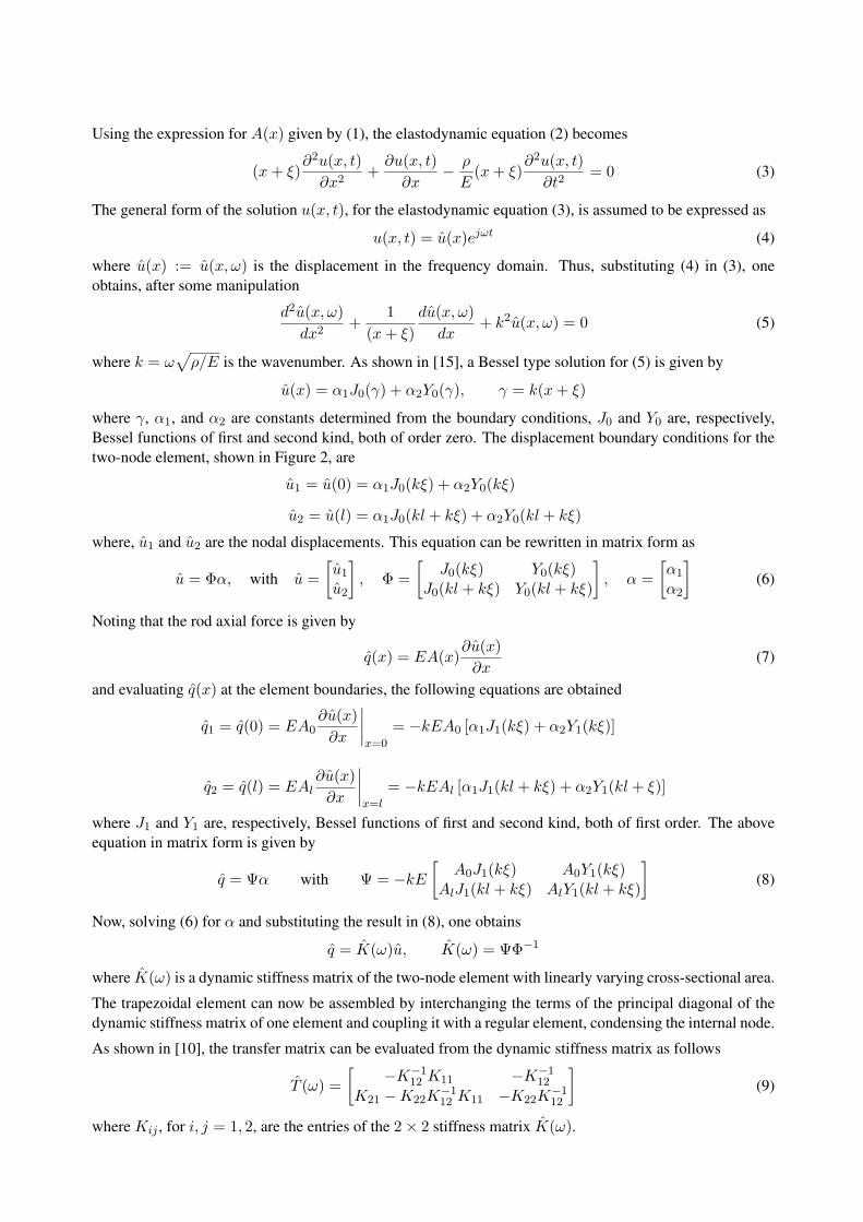
Using the expression for A(x) given by (1), the elastodynamic equation (2) becomes

(x+ ξ)∂2u(x, t)

∂x2+

∂u(x, t)

∂x− ρ

E(x+ ξ)

∂2u(x, t)

∂t2= 0 (3)

The general form of the solution u(x, t), for the elastodynamic equation (3), is assumed to be expressed as

u(x, t) = u(x)ejωt (4)

where u(x) := u(x, ω) is the displacement in the frequency domain. Thus, substituting (4) in (3), one

obtains, after some manipulation

d2u(x, ω)

dx2+

1

(x+ ξ)

du(x, ω)

dx+ k2u(x, ω) = 0 (5)

where k = ω√

ρ/E is the wavenumber. As shown in [15], a Bessel type solution for (5) is given by

u(x) = α1J0(γ) + α2Y0(γ), γ = k(x+ ξ)

where γ, α1, and α2 are constants determined from the boundary conditions, J0 and Y0 are, respectively,

Bessel functions of first and second kind, both of order zero. The displacement boundary conditions for the

two-node element, shown in Figure 2, are

u1 = u(0) = α1J0(kξ) + α2Y0(kξ)

u2 = u(l) = α1J0(kl + kξ) + α2Y0(kl + kξ)

where, u1 and u2 are the nodal displacements. This equation can be rewritten in matrix form as

u = Φα, with u =

[

u1u2

]

, Φ =

[

J0(kξ) Y0(kξ)J0(kl + kξ) Y0(kl + kξ)

]

, α =

[

α1

α2

]

(6)

Noting that the rod axial force is given by

q(x) = EA(x)∂u(x)

∂x(7)

and evaluating q(x) at the element boundaries, the following equations are obtained

q1 = q(0) = EA0∂u(x)

∂x

∣

∣

∣

∣

x=0

= −kEA0 [α1J1(kξ) + α2Y1(kξ)]

q2 = q(l) = EAl∂u(x)

∂x

∣

∣

∣

∣

x=l

= −kEAl [α1J1(kl + kξ) + α2Y1(kl + ξ)]

where J1 and Y1 are, respectively, Bessel functions of first and second kind, both of first order. The above

equation in matrix form is given by

q = Ψα with Ψ = −kE

[

A0J1(kξ) A0Y1(kξ)AlJ1(kl + kξ) AlY1(kl + kξ)

]

(8)

Now, solving (6) for α and substituting the result in (8), one obtains

q = K(ω)u, K(ω) = ΨΦ−1

where K(ω) is a dynamic stiffness matrix of the two-node element with linearly varying cross-sectional area.

The trapezoidal element can now be assembled by interchanging the terms of the principal diagonal of the

dynamic stiffness matrix of one element and coupling it with a regular element, condensing the internal node.

As shown in [10], the transfer matrix can be evaluated from the dynamic stiffness matrix as follows

T (ω) =

[

−K−112 K11 −K−1

12

K21 −K22K−112 K11 −K22K

−112

]

(9)

where Kij , for i, j = 1, 2, are the entries of the 2× 2 stiffness matrix K(ω).

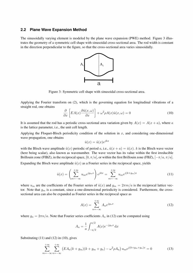
2.2 Plane Wave Expansion Method

The sinusoidally varying element is modeled by the plane wave expansion (PWE) method. Figure 3 illus-

trates the geometry of a symmetric cell shape with sinusoidal cross-sectional area. The rod width is constant

in the direction perpendicular to the figure, so that the cross-sectional area varies sinusoidally.

Figure 3: Symmetric cell shape with sinusoidal cross-sectional area.

Applying the Fourier transform on (2), which is the governing equation for longitudinal vibrations of a

straight rod, one obtains∂

∂x

[

EA(x)∂u(x, ω)

∂x

]

+ ω2ρA(x)u(x, ω) = 0 (10)

It is assumed that the rod has a periodic cross-sectional area variation given by A(x) = A(x + a), where ais the lattice parameter, i.e., the unit cell length.

Applying the Floquet-Bloch periodicity condition of the solution in x, and considering one-dimensional

wave propagation, one obtains

u(x) = u(x)ejkx

with the Bloch wave amplitude u(x) periodic of period a, i.e., u(x+ a) = u(x). k is the Bloch wave vector

(here being scalar), also known as wavenumber. The wave vector has its value within the first irreducible

Brillouin zone (FIBZ), in the reciprocal space, [0, π/a], or within the first Brillouin zone (FBZ), [−π/a, π/a].

Expanding the Bloch wave amplitude u(x) as a Fourier series in the reciprocal space, yields

u(x) =

(

+∞∑

m=−∞

umejgmx

)

ejkx =+∞∑

m=−∞

umej(k+gm)x (11)

where um are the coefficients of the Fourier series of u(x) and gm = 2πm/a is the reciprocal lattice vec-

tor. Note that gm is a constant, since a one-dimensional periodicity is considered. Furthermore, the cross-

sectional area can also be expanded as Fourier series in the reciprocal space as

A(x) =+∞∑

n=−∞

Anejgnx (12)

where gn = 2πn/a. Note that Fourier series coefficients An in (12) can be computed using

An =1

a

∫ a/2

−a/2A(x)e−jgnx dx

Substituting (11) and (12) in (10), gives

+∞∑

m=−∞

+∞∑

n=−∞

(

EAn(k + gm)(k + gm + gn)− ω2ρAn

)

umej(k+gm+gn)x = 0 (13)

Multiplying (13) by e−j(k+gr)x, with gr = 2πr/a, and integrating from −a/2 to a/2, yields

+∞∑

m=−∞

+∞∑

n=−∞

(

EAn(k + gm)(k + gm + gn)− ω2ρAn

)

um1

a

∫ a/2

−a/2ej(gm+gn−gr)x dx = 0 (14)

Given that

1

a

∫ a/2

−a/2ej(gm+gn−gr)x dx =

1

a

∫ a/2

−a/2ej2π/a(m+n−r)x dx =

{

1 , if n = r −m

0 , otherwise

one can rewrite (14) as

+∞∑

m=−∞

(

EAr−m(k + gm)(k + gr)− ω2ρAr−m

)

um = 0

Equivalently

+∞∑

m=−∞

EAr−m(k + gm)(k + gr)um = λ+∞∑

r=−∞

ρAr−mum, λ = ω2 (15)

which is a system with an infinite amount of equations. Thus, to solve this system, one can truncate the

Fourier series to the first M terms, i.e., r,m ∈ [−M, . . . ,M ] ∈ Z, such that (15) can be rewritten as

Bu = λCu (16)

where the coefficients of vector u are um and the coefficients of matrices B and C are given by

Brm = EAr−m(k + gm)(k + gr), Crm = ρAr−m

Notice that (16) represents a generalized eigenvalue problem on λ and should be solved for each k, within

FBZ or FIBZ.

2.3 State-Space Formulation

This section presents the proposed method. It shows how to write the elastodynamic equations for a rod

in a state-space formulation, to rewrite the problem in terms of the mechanical impedance and to solve a

Riccati equation to obtain the impedance at one end, given a zero impedance at the other end (free end).

It also illustrates how to obtain the transfer matrix and the dynamic stiffness matrix from the impedance.

The results obtained with this method will be referred to as state-space formulation (SSF) in the numerical

section.

Using (10) and (7), one can write the set of state-space equations

∂q(x)

∂x= −ω2ρA(x)u(x) and

∂u(x)

∂x=

q(x)

EA(x)

which can be written in matrix form as∂p

∂x= Hp (17)

with the state p(x) := p(x, ω) and H(x, ω) having the following expressions

p(x) =

[

u(x)q(x)

]

and H(x, ω) =

[

H11 H12

H21 H22

]

=

01

EA(x)−ω2ρA(x) 0

Note that this is a system of linear ordinary differential equations of the first order, where the system pa-

rameters may vary along x. It is straightforward to solve this system numerically for any type of parameter

variation along x, if the state initial condition is known. However, the initial condition is not known, since

the boundary condition at any edge of the structure is given by either the force (Neumann condition), the

displacement (Dirichlet condition), or the mechanical impedance (mixed condition). Thus, to overcome this

issue, one can rewrite the problem (see [9]) in terms of the mechanical impedance z(x), which is the relation

between the state variables u and q given by

q(x) = jωz(x)u(x) (18)

Substituting (18) into (17), one obtains the following set of equations

∂u(x)

∂x= H11u(x) +H12q(x) and jω

∂z(x)u(x)

∂x= H21u(x) +H22q(x)

which leads to

jω

(

∂z(x)

∂xu(x) + z(x)H11u(x) + z(x)H12jωz(x)u(x)

)

= H21u(x) +H22jωz(x)u(x)

Since u(x) cannot be identically zero, one finally obtains the following Riccati equation

∂z(x)

∂x+ z(x)H11 −H22z(x) + jωz(x)H12z(x) = (jω)−1H21

To solve the above Riccati differential equation, it is necessary an initial condition, which can be taken to be

z(0) = 0. This condition on a free end of the structure corresponds to the force q0 = 0, and a displacement

u0 unknown but different from zero. Once the impedance z(L), the solution of the Riccati equation at the

terminal position x = L, is computed using the initial condition z(0) = 0, the displacement u(L) can be

computed by considering that the external force in (18) is given by q(L) = 1.

With q(L) and u(L) computed, the state p(L) can be used as the initial condition in (17) so that the state

p(0) can be obtained by a backward integration of the state equations (17). Then, using the states at both

ends, given by p(0) and p(L), it is possible to compute the transfer matrix, which relates the states at the

extremes of a finite rod, as follows

p(L) = T (ω)p(0)

where T (ω) is the transfer matrix of size 2 × 2. Using the boundary conditions q(L) = 1, q(0) = 0,

u(L) = uL, and u(0) = u0, ones obtains

[

uL1

]

=

[

T11 T12

T21 T22

] [

u00

]

Solving this algebraic system of equations leads to

T11 = uL/u0, T21 = u−10

T22 = T11, (due to the rod cell symmetry)

The relation between the off diagonal terms of matrix T can be evaluated using the relation between the

transfer matrix and the symmetric (due to reciprocity) dynamic stiffness matrix, given by (9), and imposing

T11 = T22 for a symmetric cell. It can be shown that

T12 = (T 211 − I)T−1

21

Once the transfer matrix T (ω) is computed, the dynamic stiffness matrix is readily obtained using (9).

If the structure cell is not symmetric, T11 6= T22, the above formulation is unable to compute T12. In

order to overcome this issue, the initial condition is applied at the other end, x = L and the impedance is

integrated in the opposite direction up to x = 0. Repeating the procedure done earlier, one obtains p(0) and

p(L). Applying the new boundary conditions, given by q(L) = 0 and q(0) = 1, the transfer matrix relation

becomes[

u∗L0

]

=

[

T11 T12

T21 T22

] [

u∗01

]

Writing T12 and T22 in terms of T11 and T21, gives

T12 = u∗L − T11u∗

0, T22 = −T21u∗

0

where u∗L and u∗0 are the new displacement terms obtained. Now, with T11 and T21 previously obtained, the

transfer matrix and, consequently, the dynamic stiffness matrix, are obtained.

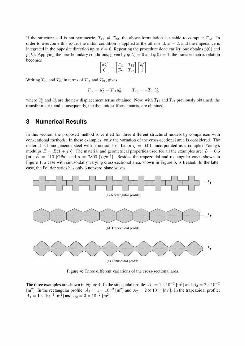
3 Numerical Results

In this section, the proposed method is verified for three different structural models by comparison with

conventional methods. In these examples, only the variation of the cross-sectional area is considered. The

material is homogeneous steel with structural loss factor η = 0.01, incorporated as a complex Young’s

modulus E = E(1 + jη). The material and geometrical properties used for all the examples are: L = 0.5[m], E = 210 [GPa], and ρ = 7800 [kg/m3]. Besides the trapezoidal and rectangular cases shown in

Figure 1, a case with sinusoidally varying cross-sectional area, shown in Figure 3, is treated. In the latter

case, the Fourier series has only 3 nonzero plane waves.

(a) Rectangular profile.

(b) Trapezoidal profile.

(c) Sinusoidal profile.

Figure 4: Three different variations of the cross-sectional area.

The three examples are shown in Figure 4. In the sinusoidal profile: A1 = 1×10−2 [m2] and A2 = 2×10−2

[m2]. In the rectangular profile: A1 = 1 × 10−2 [m2] and A2 = 2 × 10−2 [m2]. In the trapezoidal profile:

A1 = 1× 10−4 [m2] and A2 = 3× 10−2 [m2].

0 0.1 0.2 0.3 0.4 0.5−50

0

50

100

150

Length [m]

|Z(x

)| d

B r

e 1

.0 N

s/m

SSF

SEM

(a) Relative tolerance 10−2.

0 0.1 0.2 0.3 0.4 0.5−50

0

50

100

150

Length [m]

|Z(x

)| d

B r

e 1

.0 N

s/m

SSF

SEM

(b) Relative tolerance 10−4.

0 0.1 0.2 0.3 0.4 0.50

50

100

150

Length [m]

|Z(x

)| d

B r

e 1

.0 N

s/m

SSF

SEM

(c) Relative tolerance 10−9.

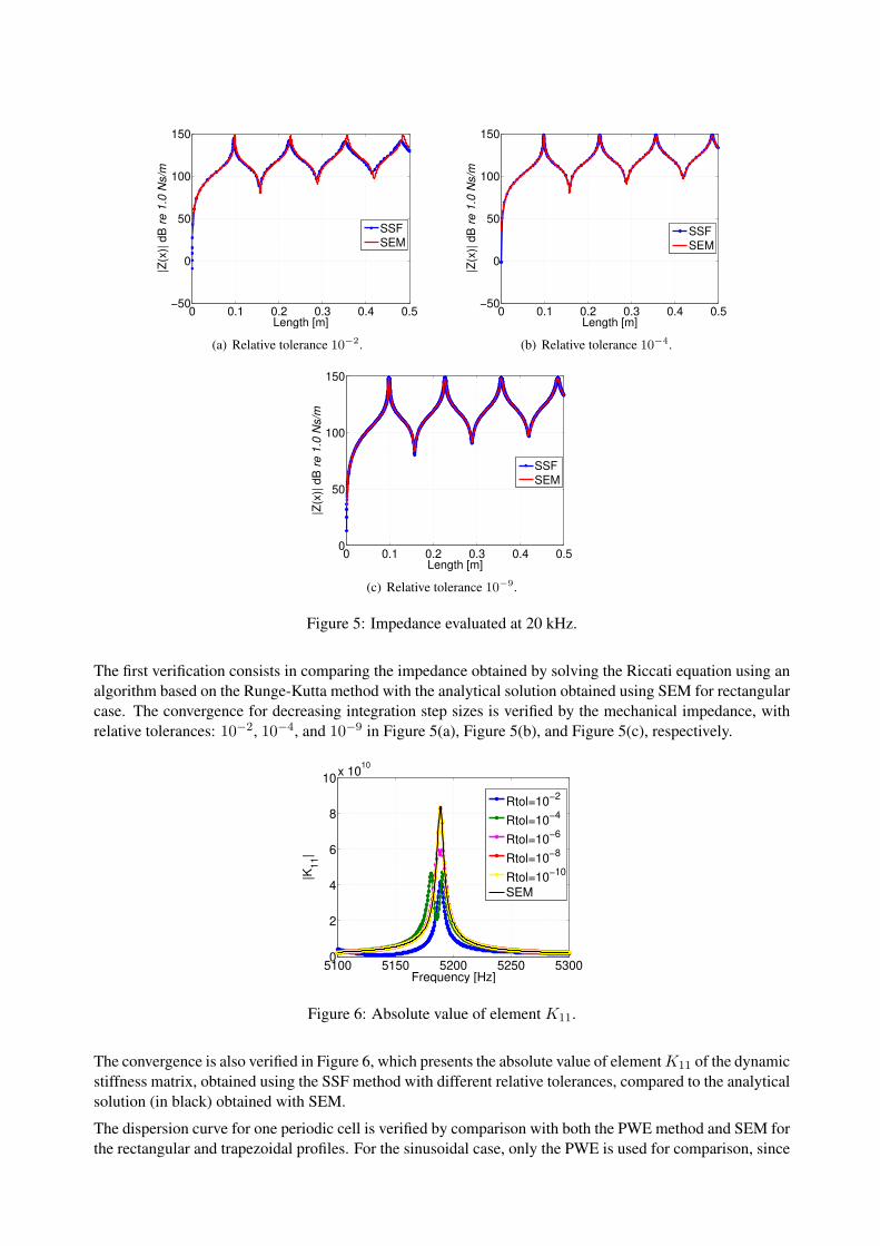
Figure 5: Impedance evaluated at 20 kHz.

The first verification consists in comparing the impedance obtained by solving the Riccati equation using an

algorithm based on the Runge-Kutta method with the analytical solution obtained using SEM for rectangular

case. The convergence for decreasing integration step sizes is verified by the mechanical impedance, with

relative tolerances: 10−2, 10−4, and 10−9 in Figure 5(a), Figure 5(b), and Figure 5(c), respectively.

5100 5150 5200 5250 53000

2

4

6

8

10x 10

10

Frequency [Hz]

|K1

1|

Rtol=10−2

Rtol=10−4

Rtol=10−6

Rtol=10−8

Rtol=10−10

SEM

Figure 6: Absolute value of element K11.

The convergence is also verified in Figure 6, which presents the absolute value of element K11 of the dynamic

stiffness matrix, obtained using the SSF method with different relative tolerances, compared to the analytical

solution (in black) obtained with SEM.

The dispersion curve for one periodic cell is verified by comparison with both the PWE method and SEM for

the rectangular and trapezoidal profiles. For the sinusoidal case, only the PWE is used for comparison, since

there is no spectral element available in the literature for this cross-sectional area variation. The agreement

is very good in all cases, see Figure 7, provided the integration step is chosen appropriately.

0 0.5 1 1.5 2

x 104

0

1

2

3

4

Frequency [Hz]

|Re

(kL

)|

SSF

SEM

(a) Real part.

0 0.5 1 1.5 2

x 104

0

0.2

0.4

0.6

0.8

Frequency [Hz]

|Im

(kL)|

SSFSEM

(b) Imaginary part.

0 0.5 1 1.5 2

x 104

0

1

2

3

4

Frequency [Hz]

|Re

(kL

)|

SSF

SEM

(c) Real part.

0 0.5 1 1.5 2

x 104

0

0.5

1

1.5

2

2.5

Frequency [Hz]

|Im

(kL)|

SSF

SEM

(d) Imaginary part.

Figure 7: Dispersion diagram for the rectangular (a,b) and trapezoidal (c,d) profiles.

The presence of band gaps can be observed in both models in Figure 7. It is noticeable that the band gap is

larger for the tapered profile, suggesting that the smoother variation of area can increase the band gap size.

Figure 8 shows the comparison between PWE and the proposed SSF method for the sinusoidally varying

cross-section.

0 5000 10000 150000

0.5

1

1.5

2

2.5

3

Frequency [Hz]

|Re

(kL

)|

PWE

SSF

Figure 8: Real part of dispersion diagram evaluated by SSF and PWE for the sinusoidal rod.

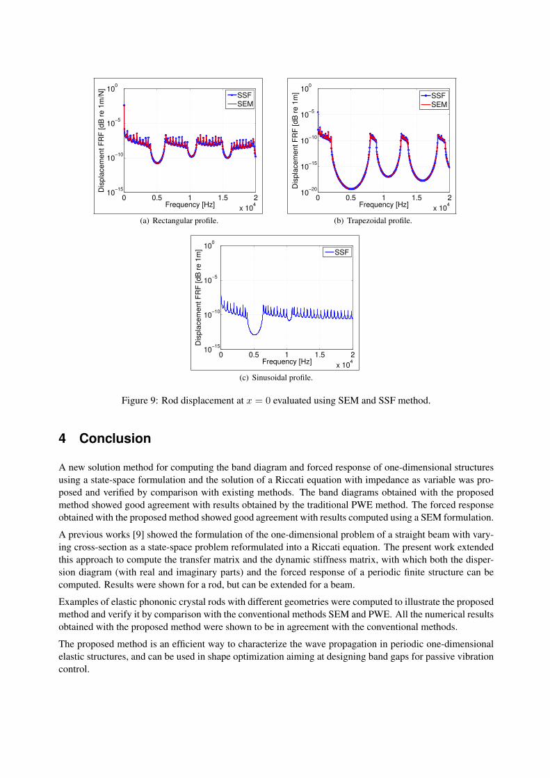
The forced response of a finite rod with ten cells is analyzed in Figure 9, considering the free-free boundary

condition and a harmonic force F = 1 [N] as excitation at the one end, at x = L. The response is measured

at the other end, at x = 0, avoiding the antiresonance and making it easier to observe the band-gap effect.

0 0.5 1 1.5 2

x 104

10−15

10−10

10−5

100

Frequency [Hz]

Dis

pla

ce

me

nt F

RF

[d

B r

e 1

m/N

]

SSFSEM

(a) Rectangular profile.

0 0.5 1 1.5 2

x 104

10−20

10−15

10−10

10−5

100

Frequency [Hz]

Dis

pla

ce

me

nt F

RF

[d

B r

e 1

m]

SSF

SEM

(b) Trapezoidal profile.

0 0.5 1 1.5 2

x 104

10−15

10−10

10−5

100

Frequency [Hz]

Dis

pla

ce

me

nt F

RF

[d

B r

e 1

m]

SSF

(c) Sinusoidal profile.

Figure 9: Rod displacement at x = 0 evaluated using SEM and SSF method.

4 Conclusion

A new solution method for computing the band diagram and forced response of one-dimensional structures

using a state-space formulation and the solution of a Riccati equation with impedance as variable was pro-

posed and verified by comparison with existing methods. The band diagrams obtained with the proposed

method showed good agreement with results obtained by the traditional PWE method. The forced response

obtained with the proposed method showed good agreement with results computed using a SEM formulation.

A previous works [9] showed the formulation of the one-dimensional problem of a straight beam with vary-

ing cross-section as a state-space problem reformulated into a Riccati equation. The present work extended

this approach to compute the transfer matrix and the dynamic stiffness matrix, with which both the disper-

sion diagram (with real and imaginary parts) and the forced response of a periodic finite structure can be

computed. Results were shown for a rod, but can be extended for a beam.

Examples of elastic phononic crystal rods with different geometries were computed to illustrate the proposed

method and verify it by comparison with the conventional methods SEM and PWE. All the numerical results

obtained with the proposed method were shown to be in agreement with the conventional methods.

The proposed method is an efficient way to characterize the wave propagation in periodic one-dimensional

elastic structures, and can be used in shape optimization aiming at designing band gaps for passive vibration

control.

Acknowledgments

The authors gratefully acknowledge the support of the Brazilian funding agencies CAPES, CNPq, FAPEMA,

and FAPESP Grant Number 14/19054-6.

References

[1] Roy R. Craig. Structural Dynamics: An Introduction to Computer Methods. John Wiley & Sons, New

York, 1981.

[2] James F. Doyle. Wave Propagation in Structures. Springer, New York, 1989.

[3] Jacques Cuenca. Wave models for the flexural vibrations of thin plates. PhD thesis, Universite du

Maine, 2009.

[4] Peter Lancaster and Leiba Rodman. Algebraic Riccati Equations. Oxford Science Publications. Claren-

don Press, 1st edition edition, 1995.

[5] J. J. Levin. On the matrix Riccati equation. Proceedings of the American Mathematical Society, 10(4):

519–524, 1959.

[6] William T. Reid. A matrix differential equation of Riccati type. American Journal of Mathematics, 68

(2):237–246, 1946.

[7] E. Davison and M. Maki. The numerical solution of the matrix Riccati differential equation. IEEE

Transactions on Automatic Control, 18(1):71–73, 1973.

[8] Charles S . Kenney and Roy B. Lepnik. Numerical integration of the differential matrix Riccati equa-

tion. IEEE Transactions on Automatic Control, 30(10):962–970, 1985.

[9] V. B. Georgiev, J. Cuenca, F. Gautier, L. Simon, and V. V. Krylov. Damping of structural vibrations in

beams and elliptical plates using the acoustic black hole effect. Journal of Sound and Vibration, 330

(11):2497–2508, 2011.

[10] P. B. Silva, J. M. Mencik, and J. R. F. Arruda. Wave finite element-based superelements for forced

response analysis of coupled systems via dynamic substructuring. International Journal for Numerical

Methods in Engineering, 107(6):453–476, 2016.

[11] M. M. Sigalas and E. N. Economou. Elastic waves in plates with periodically placed inclusions. Journal

of Applied Physics, 75(6):2845–2850, 1994.

[12] Usik Lee. Spectral Element Method in Structural Dynamics. John Wiley & Sons, New York, 2009.

[13] Khaled M. Ahmida, Jose Roberto F. Arruda, and Luiz Otavio F. Ferreira. A tapered acoustic duct

spectral element. In Proceedings of the Tenth International Congress on Sound and Vibration, 2003.

[14] G. F. C. A. Assis, J. M. C. Dos Santos, J. F. Camino, and J. R. F. Arruda. Impedance computation using

the spectral element method and the Riccati equation. In Proceedings of the 2017 CILAMCE, pages

1–9, Florianopolis, SC, Brazil, November 2017.

[15] Norman William McLachlan. Bessel Functions for Engineers. Clarendon Press Oxford, 1955.