Computing Singularly Perturbed Differential Equations∗

Sabyasachi Chatterjee† Amit Acharya‡ Zvi Artstein§

Abstract

A computational tool for coarse-graining nonlinear systems of ordinary differentialequations in time is discussed. Three illustrative model examples are worked outthat demonstrate the range of capability of the method. This includes the averagingof Hamiltonian as well as dissipative microscopic dynamics whose ‘slow’ variables,defined in a precise sense, can often display mixed slow-fast response as in relaxationoscillations, and dependence on initial conditions of the fast variables. Also coveredis the case where the quasi-static assumption in solid mechanics is violated. Thecomputational tool is demonstrated to capture all of these behaviors in an accurateand robust manner, with significant savings in time. A practically useful strategyfor accurately initializing short bursts of microscopic runs for the evolution of slowvariables is integral to our scheme, without the requirement that the slow variablesdetermine a unique invariant measure of the microscopic dynamics.

1 Introduction

This paper is concerned with a computational tool for understanding the behavior of systemsof evolution, governed by (nonlinear) ordinary differential equations, on a time scale that ismuch slower than the time scales of the intrinsic dynamics. A paradigmatic example is amolecular dynamic assembly under loads, where the characteristic time of the applied loadingis very much larger than the period of atomic vibrations. We examine appropriate theory forsuch applications and devise a computational algorithm. The singular perturbation problemswe address contain a small parameter ε that reflects the ratio between the slow and thefast time scales. In many cases, the solutions of the problem obtained by setting the smallparameter to zero matches solutions to the full problem with small ε, except in a small region -a boundary/initial layer. But, there are situations, where the limit of solutions of the originalproblem as ε tends to zero does not match the solution of the problem obtained by setting

∗To appear in Journal of Computational Physics.†Dept. of Civil & Environmental Engineering, Carnegie Mellon University, Pittsburgh, PA 15213.

sabyasac@andrew.cmu.edu.‡Dept. of Civil & Environmental Engineering, and Center for Nonlinear Analysis, Carnegie Mellon Uni-

versity, Pittsburgh, PA 15213. acharyaamit@cmu.edu.§Dept. of Mathematics, The Weizmann Institute of Science, Rehovot, Israel, 7610001.

zvi.artstein@weizmann.ac.il.

1

the small parameter to zero. Our paper covers this aspect as well. In the next section wepresent the framework of the present study, and its sources. Before displaying our algorithmin Section 6, we display previous approaches to the computational challenge. It allows us topinpoint our contribution. Our algorithm is demonstrated through computational exampleson three model problems that have been specially designed to contain the complexities intemporal dynamics expected in more realistic systems. The implementation is shown toperform robustly in all cases. These cases include the averaging of fast oscillations as well asof exponential decay, including problems where the evolution of slow variables can displayfast, almost-discontinuous, behavior in time. The problem set is designed to violate anyergodic assumption, and the computational technique deals seamlessly with situations thatmay or may not have a unique invariant measure for averaging fast response for fixed slowvariables. Thus, it is shown that initial conditions for the fast dynamics matter criticallyin many instances, and our methodology allows for the modeling of such phenomena. Themethod also deals successfully with conservative or dissipative systems. In fact, one exampleon which we demonstrate the efficacy of our computational tool is a linear, spring-mass,damped system that can display permanent oscillations depending upon delicate conditionson masses and spring stiffnesses and initial conditions; we show that our methodology doesnot require a-priori knowledge of such subtleties in producing the correct response.

2 The framework

A particular case of the differential equations we deal with is of the form

dx

dt=

1

εF (x) +G(x), (2.1)

with ε > 0 a small real parameter, and x ∈ Rn. For reasons that will become clear in thesequel we refer to the component G(x) as the drift component.

Notice that the dynamics in (2.1) does not exhibit a prescribed split into a fast and a slowdynamics. We are interested in the case where such a split is either not tractable or doesnot exist.

Another particular case where a split into a fast and slow dynamics can be identified, is alsoof interest to us, as follows.

dx

dt=

1

εF (x, l) (2.2)

dl

dt= L(x, l),

with x ∈ Rn and l ∈ Rm. We think of the variable l as a load. Notice that the dynamics ofthe load is determined by an external “slow” equation, that, in turn, may be affected by the“fast” variable x.

2

The general case we study is a combination of the previous two cases, namely,

dx

dt=

1

εF (x, l) +G(x, l) (2.3)

dl

dt= L(x, l),

which accommodates both a drift and a load. In the theoretical discussion we address thegeneral case. We display the two particular cases, since there are many interesting examplesof the type (2.1) or (2.2).

An even more general setting would be the case where the right hand side of (2.3) is of theform H(x, l, ε), namely, there is no a priori split of the right hand side of the equation intofast component and a drift or a slow component. A challenge then would be to identify,either analytically or numerically, such a split. We do not address this case here, but ourstudy reveals what could be promising directions of such a general study.

We recall that the parameter ε in the previous equation represents the ratio between theslow (or ordinary) part in the equation and the fast one. In Appendix B we examine oneof our examples, and demonstrate how to derive the dimensionless equation with the smallparameter, from the raw mechanical equation. In real world situations, ε is small yet it isnot infinitesimal. Experience teaches us, however, that the limit behavior, as ε tends to 0,of the solutions is quite helpful in understanding of the physical phenomenon and in thecomputations. This is, indeed, demonstrated in the examples that follow.

References that carry out a study of equations of the form (2.1) are, for instance, Tao,Owhadi and Marsden [TOM10], Artstein, Kevrekidis, Slemrod and Titi [AKST07], Ariel, En-gquist and Tsai [AET09a, AET09b], Artstein, Gear, Kevrekidis, Slemrod and Titi [AGK+11],Slemrod and Acharya [SA12]; conceptually similar questions implicitly arise in the work ofKevrekidis et al. [KGH+03]. The form (2.2) coincides with the Tikhonov model, see, e.g.,O’Malley [OJ14], Tikhonov, Vasileva and Sveshnikov [TVS85], Verhulst [Ver05], or Wasow[Was65]. The literature concerning this case followed, mainly, the so called Tikhonov ap-proach, namely, the assumption that the solutions of the x-equation in (2.2), for l fixed,converge to a point x(l) that solves an algebraic equation, namely, the second equationin (2.3) where the left hand side is equal to 0. The limit dynamics then is a trajectory(x(t), l(t)), evolving on the manifold of stationary points x(l). We are interested, however,in the case where the limit dynamics may not be determined by such a manifold, and mayexhibit infinitely rapid oscillations. A theory and applications alluding to such a case areavailable, e.g., in Artstein and Vigodner [AV96], Artstein [Art02], Acharya [Ach07, Ach10],Artstein, Linshiz and Titi [ALT07], Artstein and Slemrod [AS01].

3 The goal

A goal of our study is to suggest efficient computational tools that help revealing the limitbehavior of the system as ε gets very small, this on a prescribed, possibly long, interval.

3

The challenge in such computations stems from the fact that, for small ε, computing theordinary differential equation takes a lot of computing time, to the extent that it becomesnot practical. Typically, we are interested in a numerical description of the full solution,namely, the progress of the coupled slow/fast dynamics. At times, we may be satisfied withpartial information, say in the description of the progress of a slow variable, reflecting ameasurement of the underlying dynamics. To that end we first identify the mathematicalstructure of the limit dynamics on the given interval. The computational algorithm willreveal an approximation of this limit dynamics, that, in turn, is an approximation of the fullsolution for arbitrarily small ε. If only a slow variable is of interest, it can be derived fromthe established approximation.

4 The limit dynamics

In order to achieve the aforementioned goal, we display the limit structure, as ε→ 0, of thedynamics of (2.3). To this end we identify the fast time equation

dx

dσ= F (x, l), (4.1)

when l is held fixed (recall that l may not show up at all, as in (2.1)). The equation (4.1)is the fast part of (2.3) (as mentioned, G(x) is the drift and the solution l(t) of the loadequation is the load).

Notice that when moving from (2.3) to (4.1), we have changed the time scale, with t = εσ.We refer to σ as the fast time scale.

In order to describe the limit dynamics of (2.3) we need the notions of: Probability measuresand convergence of probability measures, Young measures and convergence in the Youngmeasures sense, invariant measures and limit occupational measures. In particular, we shallmake frequent use of the fact that when occupational measures of solutions of (4.1), on longtime intervals, converge, the limit is an invariant measure of (4.1). A concise explanation ofthese notions can be found, e.g., in [AV96, AKST07].

It was proved in [AV96] for (2.2) and in [AKST07] for (2.1), that under quite general condi-tions, the dynamics converge, as ε→ 0, to a Young measure, namely, a probability measure-valued map, whose values are invariant measures of (4.1). These measures are drifted in thecase of (2.1) by the drift component of the equation, and in the case (2.2) by the load. Wedisplay the result in the general case after stating the assumptions under which the resultholds.

Assumption 4.1. The functions F (., .), G(., .) and L(., .) are continuous. The solutions, sayx(.), of the fast equation (4.1), are determined uniquely by the initial data, say x(σ0) = x0,and stay bounded for σ ≥ σ0, uniformly for x0 and for l in bounded sets.

Here is the aforementioned result concerning the structure of the limit dynamics.

Theorem 4.2. For every sequence εi → 0 and solutions (xεi(t), lεi(t)) of the perturbed equa-tion (2.3) defined on [0, T ], with (xεi(0), lεi(0)) in a bounded set, there exists a subsequence

4

εj such that (xεj(.), lεj(.)) converges as j → ∞, where the convergence in the x-coordinatesis in the sense of Young measures, to a Young measure, say µ(.), whose values are invariantmeasures of the fast equation (4.1), and the convergence in the l-coordinates is uniform onthe interval, with a limit, say l0(.), that solves the differential equation

dl

dt=

∫RnL(x, l)µ(t)dx. (4.2)

The previous general result has not been displayed in the literature, but the arguments in[AKST07] in regard to (2.1) or the proof given in [AV96] for the case (2.2), apply to thepresent setting as well.

5 Measurements and slow observables

A prime role in our approach is played by slow observables, whose dynamics can be followed.The intuition behind the notion is that the observations which the observable reveals, is aphysical quantity on the macroscopic level, that can be detected. Here we identify somecandidates for such variables. The role they play in the computations is described in thenext section.

In most generality, an observable is a mapping that assigns to a probability measure µ(t)arising as a value of the Young measure in the limit dynamics of (2.3), a real number,or a vector, say in Rk. Since the values of the Young measure are obtained as limits ofoccupational measures (that in fact we use in the computations), we also demand that theobservable be defined on these occupational measures, and be continuous when passing fromthe occupational measures to the value of the Young measure.

An observable v(.) is a slow observable if when applied to the Young measure µ(.) thatdetermines the limit dynamics in Theorems 4.2, the resulting vector valued map v(t) =v(µ(t), l(t)) is continuous at points where the measure µ(.) is continuous.

An extrapolation rule for a slow observable v(.) determines an approximation of the valuev(t + h), based on the value v(t) and, possibly, information about the value of the Youngmeasure µ(t) and the load l(t), at the time t. A typical extrapolation rule would be generatedby the derivative, if available, of the slow observable. Then v(t+ h) = v(t) + hdv

dt(t).

A trivial example of a slow observable of (2.3) with an extrapolation rule is the variable l(t)itself. It is clearly slow, and the right hand side of the differential equation (4.2) determinesthe extrapolation rule, namely :

l(t+ h) = l(t) + hdl

dt(t). (5.1)

An example of a slow observable possessing an extrapolation rule in the case of (2.1), is anorthogonal observable, introduced in [AKST07]. It is based on a mapping m(x, l) : Rn → Rwhich is a first integral of the fast equation (4.1) (with l fixed), namely, it is constant along

5

solutions of (4.1). Then we define the observable v(µ) = m(x, l) with x any point in thesupport of µ. But in fact, it will be enough to assume that the mapping m(x, l) is constant onthe supports of the invariant measures arising as values of a Young measure. The definitionof v(µ) = m(x, l) with x any point in the support of µ stays the same, that is, m(x, l) maynot stay constant on solutions away from the support of the limit invariant measure. It wasshown in [AKST07] for the case (2.1), that if m(.) is continuously differentiable, then v(t)satisfies, almost everywhere, the differential equation

dv

dt=

∫Rn∇m(x)G(x)µ(t)dx. (5.2)

It is possible to verify that the result holds also when the observable satisfies the weakercondition just described, namely, it is a first integral only on the invariant measures thatarise as values of the limit Young measure. The differential equation (5.2) is not in a closedform, in particular, it is not an ordinary differential equation. Yet, if one knows µ(t) and v(t)at time t, the differentiability expressed in (5.2) can be employed to get an extrapolation ofthe form v(t+h) = v(t) +hdv

dt(t) at points of continuity of the Young measure, based on the

right hand side of (5.2). A drawback of an orthogonal observable for practical purposes isthat finding first integrals of the fast motion is, in general, a non-trivial matter.

A natural generalization of the orthogonal observable would be to consider a moment ora generalized moment, of the measure µ(t). Namely, to drop the orthogonality from thedefinition, allowing a general m : Rn → R be a measurement (that may depend, continuouslythough, on l when l is present), and define

v(µ) =

∫Rnm(x)µ(dx). (5.3)

Thus, the observable is an average, with respect to the probability measure, of the boundedcontinuous measurement m(.) of the state. If one can verify, for a specific problem, that µ(t)is piecewise continuous, then the observable defined in (5.3) is indeed slow. The drawbackof such an observable is the lack of an apparent extrapolation rule. If, however, in a givenapplication, an extrapolation rule for the moment can be identified, it will become a usefultool in the analysis of the equation.

A generalization of (5.3) was suggested in [AS06, AET09a] in the form of running time-averages as slow variables, and was made rigorous in the context of delay equations in[SA12]. Rather than considering the average of the bounded and continuous function m(x)with respect µ(t), we suggest considering the average with respect to the values of the Youngmeasure over an interval [t−∆, t], i.e,

v(t) =1

∆

∫ t

t−∆

∫Rnm(x)µ(s)(dx)ds. (5.4)

Again, the measurement m may depend on the load. Now the observable (5.4) depends notonly on the value of the measure at t, but on the “history” of the Young measure, namely itsvalues on [t−∆, t]. The upside of the definition is that v(t) is a Lipschitz function of t (the

6

Lipschitz constant may be large when ∆ is small) and, in particular, is almost everywheredifferentiable. The almost everywhere derivative of the slow variable is expressed at thepoints t where µ(.) is continuous at t and at t−∆, by

dv

dt=

1

∆

(∫Rnm(x)µ(t)(dx)−

∫Rnm(x)µ(t−∆)(dx)

). (5.5)

This derivative induces an extrapolation rule.

For further reference we call an observable that depends on the values of the Young measureover an interval prior to t, an H-observable (where the H stands for history).

An H-observable need not be an integral of generalized moments, i.e., of integrals. Forinstance, for a given measure µ let

r(µ) = max{x · e1 : x ∈ supp(µ)}, (5.6)

where e1 is a prescribed unit vector and supp(µ) is the support of µ. Then, when supp(µ) iscontinuous in µ, (and recall Assumption 4.1) the expression

v(t) =1

∆

∫ t

t−∆r(µ(τ))dτ, (5.7)

is a slow observable, and

dv

dt=

1

∆(r(µ(t))− r(µ(t−∆))) (5.8)

determines its extrapolation rule.

The strategy we display in the next section applies whenever slow observables with validextrapolation rules are available. The advantage of the H-observables as slow variables isthat any smooth function m(.) generates a slow observable and an extrapolation rule. Plentyof slow variables arise also in the case of generalized moments of the measure, but then itmay be difficult to identify extrapolation rules. The reverse situation occurs with orthogonalobservables. It may be difficult to identify first integrals of (4.1), but once such an integralis available, its extrapolation rule is at hand.

Also note that in all the preceding examples the extrapolation rules are based on deriva-tives. We do not exclude, however, cases where the extrapolation is based on a differentargument. For instance, on information of the progress of some given external parameter,for instance, a control variable. All the examples computed in the present paper will useH-observables.

6 The algorithm

Our strategy is a modification of a method that has been suggested in the literature andapplied in some specific cases. We first describe these, as it will allow us to pinpoint ourcontribution.

7

A computational approach to the system (2.2) has been suggested in Vanden-Eijnden [VE03]and applied in Fatkullin and Vanden-Eijnden [FVE04]. It applies in the special case wherethe fast process is stochastic, or chaotic, with a unique underlying measure that may dependon the load. The underlying measure is then the invariant measure arising in the limitdynamics in our Theorem 4.2. It can be computed by solving the fast equation, initializingit at an arbitrary point. The method carried out in [VE03] and [FVE04] is, roughly, asfollows. Suppose the value of the slow variable (the load in our terminology) at time t isknown. The fast equation is run then until the invariant measure is revealed. The measure isthen employed in the averaging that determines the right hand side of the slow equation att, allowing to get a good approximation of the load variable at t+ h. Repeating this schemeresults in a good approximation of the limit dynamics of the system. The method relies on theproperty that the value of the load determines the invariant measure. The latter assumptionhas been lifted in [ALT07], analyzing an example where the dynamics is not ergodic andthe invariant measure for a given load is not unique, yet the invariant measure appearingin the limit dynamics can be detected by a good choice of an initial condition for the fastdynamics. The method is, again, to alternate between the computation of the invariantmeasure at a given time, say t, and using it then in the averaging needed to determine theslow equation. Then determine the value of the load at t+ h. The structure of the equationallows to determine a good initial point for computing the invariant measure at t + h, andso on and so forth, until the full dynamics is approximated.

The weakness of the method described in the previous paragraph is that it does not applywhen the split to fast dynamics and slow dynamics, i.e. the load, is not available, and evenwhen a load is there, it may not be possible to determine the invariant measure using thevalue of the load.

Orthogonal observables were employed in [AKST07] in order to analyze the system (2.1), anda computational scheme utilizing these observables was suggested. The scheme was appliedin [AGK+11]. The suggestion in these two papers was to identify orthogonal observableswhose values determine the invariant measure, or at least a good approximation of it. Oncesuch observables are given, the algorithm is as follows. Given an invariant measure at t,the values of the observables at t + h can be determined based on their values at t and theextrapolation rule based on (5.2). Then a point in Rn should be found, which is compatiblewith the measurements that define the observables. This point would be detected as asolution of an algebraic equation. Initiating the fast equation at that point and solving it ona long fast time interval, reveals the invariant measure. Repeating the process would resultin a good approximation of the full dynamics.

The drawback of the previous scheme is the need to find orthogonal observables, namelymeasurements that are constant along trajectories within the invariant measures in the limitof the fast flow, and verify that their values determine the value of the Young measure, or atleast a good approximation of it. Also note that the possibility to determine the initializationpoint with the use of measurements, rather than the observables, relies on the orthogonality.Without orthogonality, applying the measurements to the point of initialization of the fastdynamics, yields no indication. In this connection, it is important to mention the work ofAriel, Engquist, and Tsai [AET09a, AET09b] that demonstrates theory, and computations

8

utilizing the Hetergeneous Multiscale Modeling (HMM) scheme of E and Engquist [EE03],for defining a complete set of slow variables that determine the unique invariant measure formicroscopic systems equipped with such.

The scheme that we suggest employs general observables with extrapolation rules. As men-tioned, there are plenty of these observables, in particular H-observables, as (5.4) indicates.The scheme shows how to use them in order to compute the full dynamics, or a good ap-proximation of it.

It should be emphasized that none of our examples satisfy the ergodicity assumption placedin the aforementioned literature. Also, in none of the examples it is apparent, if possible atall, to find orthogonal observables. In addition, our third example exhibits extremely rapidvariation in the slow variable (resembling a jump), a phenomenon not treated in the relevantliterature so far.

We provide two versions of the scheme. One for observables determined by the values µ(t)of the Young measure, and the second for H-observables, namely, observables depending onthe values of the Young measure over an interval [t−∆, t]. The modifications needed in thelatter case are given in parentheses.

The scheme. Consider the full system (2.3), with initial conditions x(t0) = x0 and l(t0) = l0.Our goal is to produce a good approximation of the limit solution, namely the limit Youngmeasure µ(.), on a prescribed interval [t0, T0].

A general assumption. The function of time defined by the closest-point projection, insome appropriate metric, of any fixed point in state-space on the support of µ(t) for eacht in any interval in which µ(·) is continuous, is smooth. A number of slow observables, sayv1, . . . , vk can be identified, each of them equipped with an extrapolation rule, valid at allcontinuity points of the Young measure.

Initialization of the algorithm. Solve the fast equation (4.1) with initial condition x0 anda fixed initial load l0, long enough to obtain a good approximation of the value of the Youngmeasure at t0. (In the case of an H-observable solve the full equation with ε small, on aninterval [t0, t0 +∆], with ε small enough to get a good approximation of the Young measureon the interval). In particular the initialization produces good approximations of µ(t) fort = t0 (for t = t0 +∆ in case of an H-observable). Compute the values v1(µ(t)), ..., vk(µ(t))of the observables at this time t.

The recursive part.

Step 1: We assume that at time t the values of the observables v1(µ(t)), ..., vk(µ(t)), appliedto the value µ(t) of the Young measure, are known. We also assume that we have enoughinformation to invoke the extrapolation rule to these observables (for instance, we can com-pute dv

dtwhich determines the extrapolation when done via a derivative). If the model has a

load variable, it should be one of the observables.

Step 2: Apply the extrapolation rule to the observables and get an approximation of thevalues v1(µ(t + h)), ..., vk(µ(t + h)), of the observables at time t + h (time t + h−∆ in thecase of an H-observable). Denote the resulting approximation by (v1, ..., vk).

9

Step 3: Make an intelligent guess of a point x(t + h) (or x(t + h − ∆) in the case of H-observable), that is in the basin of attraction of µ(t + h) (or µ(t + h − ∆) in the case ofH-observable). See a remark below concerning the intelligent guess.

Step 4: Initiate the fast equation at (x(t + h), l(t + h)) and run the equation until a goodapproximation of an invariant measure arises (initiate the full equation, with small ε at(x(t+ h−∆), l(t+ h−∆)), and run it on [t+ h−∆, t+ h], with ε small enough such thata good approximation for a Young measure on the interval is achieved).

Step 5: Check if the invariant measure µ(t+h) revealed in the previous step is far from µ(t)(this step, and consequently step 6.1, should be skipped if the Young measure is guaranteedto be continuous).

Step 6.1: If the answer to the previous step is positive, it indicates that a point of discon-tinuity of the Young measure may exist between t and t+ h. Go back to t and compute thefull equation (initiating it with any point on the support of µ(t)) on [t, t + h], or until thediscontinuity is revealed. Then start the process again at Step 1, at the time t + h (or at atime after the discontinuity has been revealed).

Step 6.2: If the answer to the previous step is negative, compute the values of the ob-servables v1(µ(t + h)), ..., vk(µ(t + h)) at the invariant measure that arises by running theequation. If there is a match, or almost a match, with (v1, ..., vk), accept the value µ(t+ h)(accept the computed values on [t+h−∆, t+h] in the case of an H-observable) as the valueof the desired Young measure, and start again at Step 1, now at time t+ h. If the match isnot satisfactory, go back to step 3 and make an improved guess.

Conclusion of the algorithm. Continue with steps 1 to 6 until an approximation of theYoung measure is computed on the entire time interval [t0, T0].

Making the intelligent guess in Step 3. The goal in this step is to identify a point in thebasin of attraction of µ(t+ h). Once a candidate for such a point is suggested, the decisionwhether to accept it or not is based on comparing the observables computed on the invariantmeasure generated by running the equation with this initial point, to the values as predictedby the extrapolation rule. If there is no match, we may improve the initial suggestion forthe point we seek.

In order to get an initial point, we need to guess the direction in which the invariant measureis drifted. We may assume that the deviation of µ(t+h) from µ(t) is similar to the deviationof µ(t) from µ(t− h). Then the first intelligent guess would be, say, a point xt+h such thatxt+h − xt = xt − xt−h where xt is a point in the support of µ(t) and xt−h is the point in thesupport of µ(t− h) closest, or near closest, to xt. At this point, in fact, we may try severalsuch candidates, and check them in parallel. If none fits the criterion in Step 6.2, the processthat starts again at Step 3, could use the results in the previous round, say by perturbingthe point that had the best fit in a direction of, hopefully, a better fit. A sequence of betterand better approximations can be carried out until the desired result is achieved.

10

7 The expected savings in computer time

The motivation behind our scheme of computations is that the straightforward approach,namely, running the entire equation (2.3) on the full interval, is not feasible if ε is very small.To run (4.1) in order to compute the invariant measure at a single point t, or to run (2.3) ona short interval [t−∆, t], with ∆ small, does not consume a lot of computing time. Thus, ourscheme replaces the massive computations with computing the values of the Young measureat a discrete number of points, or short intervals, and the computation of the extrapolationrules to get an estimate of the progress of the observables. The latter step does not dependon ε, and should not consume much computing time. Thus, if h is large (and large relativeto ∆ in the case of H-observables), we achieve a considerable saving.

These arguments are also behind the saving in the cited references, i.e., [VE03, FVE04,ALT07, AGK+11]. In our algorithm there is an extra cost of computing time, namely, theneed to detect points in the basin of attraction of the respective invariant measures, i.e., Step3 in our algorithm. The extra steps amount to, possibly, an addition of a discrete numberof computations that reveal the invariant measures. An additional computing time may beaccrued when facing a discontinuity in the Young measure. The cost is, again, a computationof the full Young measure around the discontinuity. The possibility of discontinuity has notbeen address in the cited references.

8 Error estimates

The considerations displayed and commented on previously were based on the heuristicsbehind the computations. Under some strong, yet common, conditions on the smoothnessof the processes, one can come up with error estimate for the algorithm. We now producesuch an estimate, which is quite standard (see e.g., [BFR78]). Of interest here is the natureof assumptions on our process, needed to guarantee the estimate.

Suppose the computations are performed on a time interval [0, T ], with time steps of length h.The estimate we seek is the distance between the computed values, say P (kh), k = 0, 1, ..., N,of invariant measures, and the true limit dynamics, that is the values µ(kh) of the limit Youngmeasure, at the same mesh points (here hN is close to T ).

Recall that the Young measure we compute is actually the limit as ε → 0 of solutions of(2.3). Still, we think of µ(t) as reflecting a limiting dynamics, and consider the value µ(0) asits initial state, in the space of invariant measures (that may indeed be partially supportedon points, for instance, in case the load is affected by the dynamics, we may wish to computeit as well). We shall denote by µ(h, ν) the value of the Young measure obtained at the timeh, had ν been the initial state. Likewise, we denote by P (h, ν) the result of the computationsat time h, had ν been the invariant measure to which the algorithm is applied. We placethe assumptions on µ(h, ν) and P (h, ν). After stating the assumption we comment on thereflection of them on the limit dynamics and the algorithm. Denote by ρ(., .) a distance, saythe Prohorov metric, between probability measures.

11

Assumption 8.1. There exists a function δ(h), continuous at 0 with δ(0) = 0, and aconstant η such that

ρ(P (h, ν), µ(h, ν)) ≤ δ(h)h, (8.1)

and

ρ(µ(h, ν1), µ(h, ν2)) ≤ (1 + ηh)ρ(ν1, ν2). (8.2)

Remark. Both assumptions relate to some regularity of the limiting dynamics. The in-equality (8.2) reflects a Lipschitz property. It holds, for instance, in case µ(t) is a solutionof an ordinary differential equations with Lipschitz right hand side. Recall that without aLipschitz type condition it is not possible to get reasonable error estimates even in the odeframework. Condition (8.1) reflects the accuracy of our algorithm on a time step of length h.For instance, If a finite set of observables determines the invariant measure, if the extrapo-lation through derivatives are uniform, if the mapping that maps the measures to the valuesof the observables is bi-Lipschitz, and if the dynamics µ(t) is Lipschitz, then (8.1) holds. Inconcrete examples it may be possible to check these properties directly (we comment on thatin the examples below).

Theorem 8.2. Suppose the inequalities in Assumption 8.1 hold. Then

ρ(P (kh), µ(kh)) ≤ δ(h)η−1(eηT − 1). (8.3)

Proof. Denote Ek = ρ((P (kh), µ(kh)), namely, Ek is the error accrued from 0 to the timekh. Then E0 = 0. Since P (kh) = P (h, P ((k− 1)h)) and µ(kh) = µ(h, µ((k− 1)h)) it followsthat

Ek ≤ ρ(P (h, P ((k − 1)h)), µ(h, P ((k − 1)h)))+

ρ(µ(h, P ((k − 1)h)), µ(h, µ((k − 1)))). (8.4)

From inequalities (8.1) and (8.2) we get

Ek ≤ δ(h)h+ (1 + ηh)Ek−1. (8.5)

Spelling out the recursion we get

Ek ≤ δ(h)h(1 + (1 + ηh) + (1 + ηh)2 + ...+ (1 + ηh)k−1)

= δ(h)η−1((1 + ηh)k − 1). (8.6)

Since hk ≤ T the claimed inequality (8.3) follows.

Remark. The previous estimate imply that the error tends to zero as the step size h tendsto zero. Note, however, that the bigger the step size, the bigger the saving of computationaltime is. This interplay is common in computing in general.

Remark. Needless to say, the previous estimate refers to the possible errors on the theo-retical dynamics of measures. A different type of errors that occur relates to the numericsof representing and approximating the measures. The same issue arises in any numericalanalysis estimates, but they are more prominent in our framework due to the nature of thedynamics.

12

9 Computational Implementation

We are given the initial conditions of the fine and the slow variables, x(−∆) = x0 andl(−∆) = l0. We aim to produce a good approximation, of the limit solution in the period[0, T0]. Due to the lack of algorithmic specification for determining orthogonal observables,we concentrate on H-observables in this paper.

In the implementation that follows, we get to the specifics of how the calculations are carriedout. Recall that the H-observables are averages of the form

v(t) =1

∆

∫ t

t−∆

∫Rnm(x)µ(s)(dx)ds. (9.1)

Namely, the H-observables are slow variables with a time-lag, i.e. the fine/microscopicsystem needs to have run on an interval of length ∆ before the observable at time t can bedefined.

From here onwards, with some abuse of notation, whenever we refer to only a measure atsome instant of time we mean the value of the Young measure of the fast dynamics at thattime. When we want to refer to the Young measure, we mention it explicitly.

We will also refer to any component of the list of variables of the original dynamics (2.3) asfine variables.

We think of the calculations marching forward in the slow time-scale in discrete steps of sizeh with T0 = nh. Thus the variable t below in the description of our algorithm takes valuesof 0h, 1h, 2h, . . . , nh.

Step 1: Calculate the rate of change of slow variableWe calculate the rate of change of the slow variable at time t using the following:

dv

dt(t) =

1

∆

(∫Rnm(x)µ(t)(dx)−

∫Rnm(x)µ(t−∆)(dx)

). (9.2)

Let us denote the term∫Rnm(x)µ(t)(dx) as Rm

t and the term∫Rnm(x)µ(t−∆)(dx) as Rm

t−∆.The term Rm

t is computed as

Rmt =

1

Nt

Nt∑i=1

m(xε(σi), lε(σi)). (9.3)

The successive values (xε(σi), lε(σi)) are obtained by running the fine system

dxεdσ

= F (xε, lε) + εG(xε, lε)

dlεdσ

= εL(xε, lε),

(9.4)

with initial condition xguess(σ = tε) and l(σ = t

ε).

13

We discuss in Step 5 how we obtain xguess(σ). Here, Nt is the number of increments takenfor the value of Rm

t to converge upto a specified value of tolerance. Also, Nt is large enoughsuch that the effect of the initial transient does not affect the value of Rm

t .

Similarly, Rmt−∆ is computed as:

Rmt−∆ =

1

Nt−∆

Nt−∆∑i=1

m (xε(σi), lε(σi)) , (9.5)

where successive values xε(σi) are obtained by running the fine system (9.4) with initialcondition xguess(σ − ∆

ε) and l(σ − ∆

ε).

We discuss in Step 3 how we obtain xguess(σ − ∆ε). Here, Nt−∆ is the number of increments

taken for the value of Rmt−∆ to converge upto a specified value of tolerance.

Step 2: Find the value of slow variableWe use the extrapolation rule to obtain the predicted value of the slow variable at the timet+ h:

v(t+ h) = v(t) +dv

dt(t)h, (9.6)

where dvdt

(t) is obtained from (9.2).

Step 3: Determine the closest point projectionWe assume that the closest-point projection of any fixed point in the fine state space, on theYoung measure of the fine evolution, evolves slowly in any interval where the Young measureis continuous. We use this idea to define a guess xguess(t + h − ∆), that is in the basin ofattraction of µ(t + h − ∆). The fixed point, denoted as xarbt−∆, is assumed to belong to theset of points, xε(σi) for which the value of Rm

t−∆ in (9.5) converged. Specifically, we makethe choice of xarbt−∆ as xε(σNt−∆) where xε(σi) is defined in (9.5) and Nt−∆ is defined in thediscussion following it. Next, we compute the closest point projection of this point (in theEuclidean norm) on the support of the measure at t− h−∆. This is done as follows.

Define xconvt−h−∆ as the point xε(σNt−h−∆), where xε(σi) is defined in the discussion surrounding(9.5) with σ replaced by σ− h

ε, and Nt−h−∆ is the number of increments taken for the value

of Rmt−h−∆ to converge (the value of xconvt−h−∆ is typically stored in memory during calculations

for the time t − h − ∆). The fine system (9.4) with σ replaced by σ − hε

is initiated fromxconvt−h−∆, and we calculate the distance of successive points on this trajectory with respectto xarbt−∆ until a maximum number of increments have been executed. We set the maximumnumber of increments as 2Nt−h−∆. The point(s) on this finite time trajectory that recordsthe smallest distance from xarbt−∆ is defined as the closest point projection, xcpt−h−∆.

Finally, the guess, xguess(t+ h−∆) is given by

xguess(t+ h−∆) = 2xarbt−∆ − xcpt−h−∆,

14

for t > 0 (see Remark associated with Step 3 in Sec. 6). For t = 0, we set

xguess(h−∆) = xarb0 +(xarb0 − x

cp−∆)

∆(h−∆),

where xarb. and xcp. are defined in the first and the second paragraph respectively in Step3 above with the time given by the subscripts. This is because the computations start att = −∆ and we do not have a measure at t = −h−∆ and hence cannot compute xcp−h−∆ tobe able to use the above formula to obtain xguess(t+ h−∆).

Thus, the implicit assumption is that xguess(t + h − ∆) is the closest-point projection ofxarbt−∆ on the support of the measure µ(t+ h−∆), and that there exists a function xcp(s) fort− h−∆ ≤ s ≤ t + h−∆ that executes slow dynamics in the time interval if the measuredoes not jump within it.

Step 4: Accept the measureWe initiate the fine equation (9.4) at (xguess(t+ h−∆), l(t+ h−∆)) and run the equationfrom σ + h

ε− ∆

εto σ + h

ε(recall σ = t

ε). We say that there is a match in the value of a slow

variable if the following equality holds (approximately):

v(t+ h) =1

N ′

N ′∑i=1

m (xε(σi), lε(σi)) , (9.7)

where v(t+ h) refers to the predicted value of the slow variable obtained from the extrapo-lation rule in Step 2 above. The successive values (xε(σi), lε(σi)) are obtained from system(9.4). Here, N ′ = ∆

ε∆σwhere ∆σ is the fine time step.

If there is a match in the value of the slow variable, we accept the measure which is generated,in principle, by running the fine equation (9.4) with the guess xguess(t + h − ∆) and moveon to the next coarse increment.

If not, we check if there is a jump in the measure. We say that there is a jump in themeasure if the value of Rm

t+h is significantly different from the value of Rmt . This can be

stated as: ∣∣∣∣Rmt+h −Rm

t

Rmt

∣∣∣∣� 1

N

∑n

∣∣∣∣Rmt−(n−1)h −Rm

t−nh

Rmt−nh

∣∣∣∣ , (9.8)

where n is such that there is no jump in the measure between t− nh and t− (n− 1)h andN is the maximal number of consecutive (integer) values of such n.

If there is no jump in the measure, we try different values of xguess(t + h − ∆) based ondifferent values of xarbt−∆ and repeat Steps 3 and 4.

If there is a jump in the measure, we declare v(t+ h) to be the the right-hand-side of (9.7).The rationale behind this decision is the assumption xguess(t + h − ∆) lies in the basin ofattraction of the measure at t+ h−∆.

15

Step 5: Obtain fine initial conditions for rate calculationStep 1 required the definition of xguess(t). We obtain it as

xguess(t) = xarbt−∆ +

(xarbt−∆ − x

cpt−h)

(h−∆)∆,

for t > 0, and xarb. and xcp. are defined in the same way as in Step 3, but at different timesgiven by the subscripts. For t = 0, we obtain xguess(0), which is required to compute Rm

0 , byrunning the fine equation (9.4) from σ = −∆

εto σ = 0. This is because the computations

start at t = −∆ and we do not have a measure at t = −h and hence cannot compute xcp−h tobe able to use the above formula to obtain xguess(t).

Another possible way to obtain xguess(t) is using the same extrapolation rule used in Step3 to obtain xguess(t + h − ∆) which means we can also obtain xguess(t) as xguess(t) =

xarbt−h−∆ +(xarbt−h−∆−x

cpt−2h−∆)

h(h + ∆). But we have not used it in the computational results

that follow.

We continue in this manner until an approximation of slow observables is computed on theentire time interval [0, T0].

Discussion. The use of the guess for fine initial conditions to initiate the fine system tocompute Rm

t+h and Rmt+h−∆ is an integral part of this implementation. This allows us to sys-

tematically use the coarse evolution equation (9.2). This feature is a principal improvementover previous work [TAD13, TAD14].

We will refer to this scheme, which is a mixture of rigorous and heuristic arguments, asPractical Time Averaging (PTA) and we will refer to results from the scheme by the samename. Results obtained solely by running the complete system will be referred to as fineresults, indicated by the superscript or subscript f when in a formula.

Thus, if v is a scalar slow variable, then we denote the slow variable value obtained usingPTA scheme as vPTA while the slow variable value obtained by running the fine system aloneis called vf .

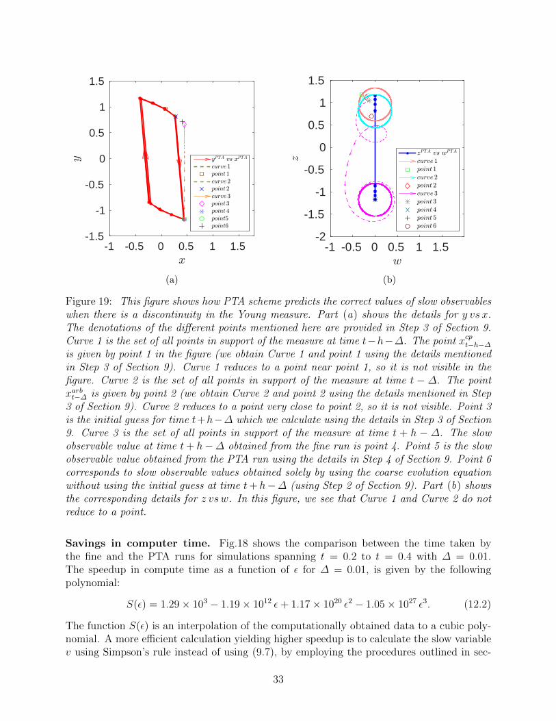
The speedup, S(ε), in compute time between the fine and PTA calculations is presentedin the results that follow in subsequent sections. This is defined to be the ratio of the timetaken by the fine calculations to that by the PTA calculations for an entire simulation, sayconsisting of n steps of size h on the slow time-scale.

Let T cpuf (ε) and T cpuPTA(ε) be the compute times to obtain the fine and PTA results per jumpon the slow time scale, respectively, for the specific value of ε. The compute time to obtainthe PTA results for n jumps in the slow time scale is nT cpuPTA(ε) which can be written as

nT cpuPTA(ε) = nT cpuPTA,1(ε) + T cpuPTA,2(ε),

where T cpuPTA,1(ε) is the compute time to perform the computations mentioned in Step 1 toStep 5 for every jump in the slow time scale. Since we cannot use the formula for xguess(t)mentioned in Step 5 to obtain xguess(0) and we have to run the fine equation (9.4) from

16

σ = −∆ε

to σ = 0, an additional overhead is incurred in the compute time for the PTAcomputations which we denote as T cpuPTA,2(ε). Thus

S(ε) =nT cpuf (ε)

nT cpuPTA(ε)≈

T cpuf (ε)

T cpuPTA,1(ε).

for large n.

Error in the PTA result is defined as:

Error(%) =vPTA − vf

vf× 100. (9.9)

We obtain vf as follows:

Step 1: We run the fine system (9.4) from σ = −∆ε

to σ = T0ε

using initial conditions (x0,l0) to obtain (xε(σi), lε(σi)) where σi = i∆σ and i ∈ Z+ and i ≤ T0+∆

ε∆σ.

Step 2: We calculate vf (t) using:

vf (t) =1

N ′

N0(t)+N ′∑i=N0(t)

m (xε(σi), lε(σi)) , (9.10)

where N ′ = ∆ε∆σ

and N0(t) = t+∆ε∆σ

where ∆σ is the fine time step.

Remark. If we are aiming to understand the evolution of the slow variables in the slowtime scale, we need to calculate them, which we do in Step 2. However, the time takenin computing the average of the state variables in Step 2 is much smaller compared to thetime taken to run the fine system in Step 1. We will show this in the results sections thatfollow.

Remark. All the examples computed in this paper employ H-observables. When, however,orthogonal observables are used, the time taken to compute their values using the PTAscheme (T cpuPTA) will not depend on the value of ε.

10 Example I: Rotating planes

Consider the following four-dimensional system, where we denote by x the vector x =(x1, x2, x3, x4).

dx

dt=F (x)

ε+G(x), (10.1)

where:

F (x) = ((1− |x|)x+ γ(x)) (10.2)

17

with

γ(x) = (x3, x4,−x1,−x2). (10.3)

The drift may be determined by an arbitrary function G(x). For instance, if we let

G(x) = (−x2, x1, 0, 0), (10.4)

then we should expect nicely rotating two-dimensional planes. A more complex drift mayresult in a more complex dynamics of the invariant measures, namely the two dimensionallimit cycles.

10.1 Discussion

The right hand side of the fast equation has two components. The first drives each point xwhich is not the origin, toward the sphere of radius 1. The second, γ(x), is perpendicular tox. It is easy to see that the sphere of radius 1 is invariant under the fast equation. For anyinitial condition x0 on the sphere of radius 1, the fast time equation is

x =

0 0 1 00 0 0 1−1 0 0 00 −1 0 0

x . (10.5)

It is possible to see that the solutions are periodic, each contained in a two dimensionalsubspace. An explicit solution (which we did not used in the computations) is

x = cos (t)

x0,1

x0,2

x0,3

x0,4

+ sin (t)

x0,3

x0,4

−x0,1

−x0,2

. (10.6)

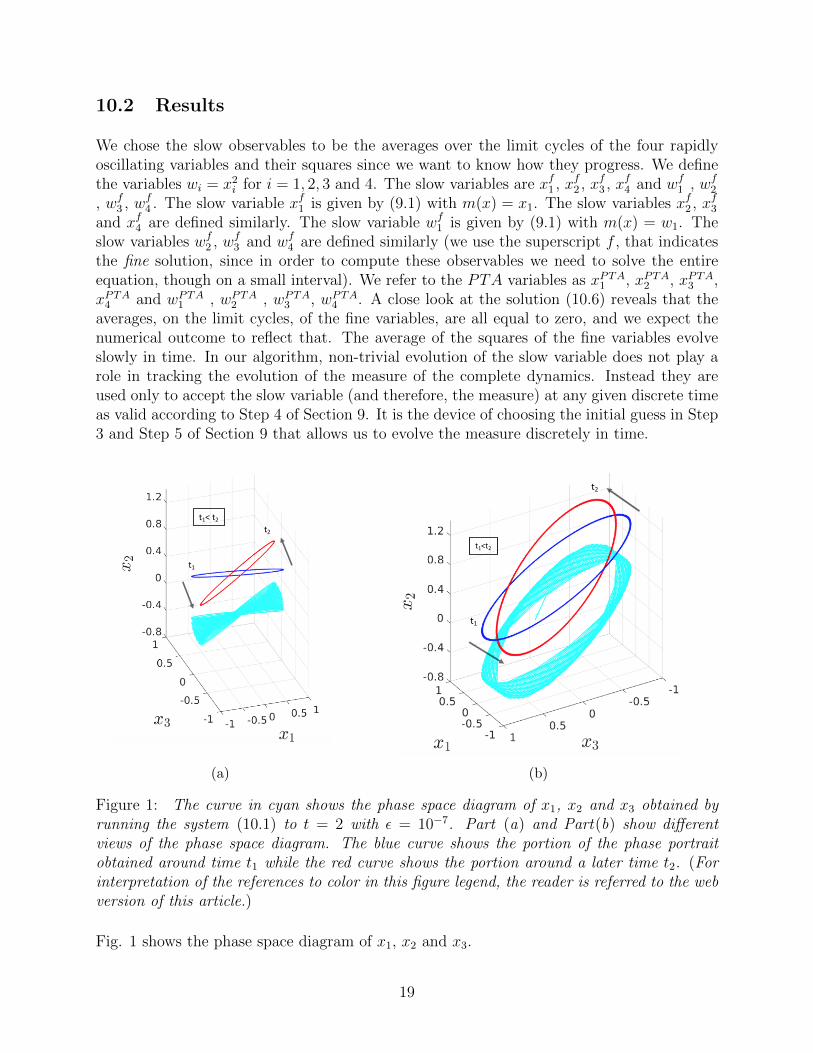
Thus, the solution at any point of time is a linear combination of x0 and γ(x0) and stays inthe plane defined by them. Together with the previous observation we conclude that the limitoccupational measure of the fast dynamics should exhibit oscillations in a two-dimensionalsubspace of the four-dimensional space. The two dimensional subspace itself is drifted bythe drift G(x). The role of the computations is then to follow the evolution of the oscillatorytwo dimensional limit dynamics.

We should, of course, take advantage of the structure of the dynamics that was revealed inthe previous paragraph. In particular, it follows that three observables of the form r(µ) givenin (5.6), with e1, e2 and e3 being unit vectors in R4, determine the invariant measure. Theyare not orthogonal (it may be very difficult to find orthogonal observables in this example),hence we may use, for instance, the H-observables introduced in (5.7).

It is also clear that the circles that determine the invariant measures move smoothly withthe planes. Hence employing observables that depend smoothly on the planes would implythat conditions (8.1) and (8.2) hold, validating the estimates of Theorem 8.2.

18

10.2 Results

We chose the slow observables to be the averages over the limit cycles of the four rapidlyoscillating variables and their squares since we want to know how they progress. We definethe variables wi = x2

i for i = 1, 2, 3 and 4. The slow variables are xf1 , xf2 , xf3 , xf4 and wf1 , wf2, wf3 , wf4 . The slow variable xf1 is given by (9.1) with m(x) = x1. The slow variables xf2 , xf3and xf4 are defined similarly. The slow variable wf1 is given by (9.1) with m(x) = w1. Theslow variables wf2 , wf3 and wf4 are defined similarly (we use the superscript f , that indicatesthe fine solution, since in order to compute these observables we need to solve the entireequation, though on a small interval). We refer to the PTA variables as xPTA1 , xPTA2 , xPTA3 ,xPTA4 and wPTA1 , wPTA2 , wPTA3 , wPTA4 . A close look at the solution (10.6) reveals that theaverages, on the limit cycles, of the fine variables, are all equal to zero, and we expect thenumerical outcome to reflect that. The average of the squares of the fine variables evolveslowly in time. In our algorithm, non-trivial evolution of the slow variable does not play arole in tracking the evolution of the measure of the complete dynamics. Instead they areused only to accept the slow variable (and therefore, the measure) at any given discrete timeas valid according to Step 4 of Section 9. It is the device of choosing the initial guess in Step3 and Step 5 of Section 9 that allows us to evolve the measure discretely in time.

t1

t2t1<t2

(a)

t1

t2

t1<t2

(b)

Figure 1: The curve in cyan shows the phase space diagram of x1, x2 and x3 obtained byrunning the system (10.1) to t = 2 with ε = 10−7. Part (a) and Part(b) show differentviews of the phase space diagram. The blue curve shows the portion of the phase portraitobtained around time t1 while the red curve shows the portion around a later time t2. (Forinterpretation of the references to color in this figure legend, the reader is referred to the webversion of this article.)

Fig. 1 shows the phase space diagram of x1, x2 and x3.

19

t0 0.02 0.04 0.06 0.08 0.1

-1.5

-1

-0.5

0

0.5

1

1.5x1

-nePTA

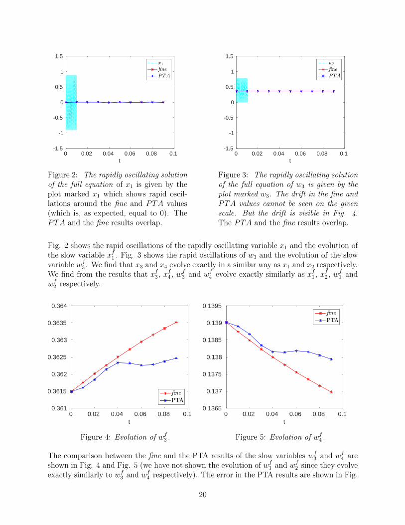
Figure 2: The rapidly oscillating solutionof the full equation of x1 is given by theplot marked x1 which shows rapid oscil-lations around the fine and PTA values(which is, as expected, equal to 0). ThePTA and the fine results overlap.

t0 0.02 0.04 0.06 0.08 0.1

-1.5

-1

-0.5

0

0.5

1

1.5w3

-nePTA

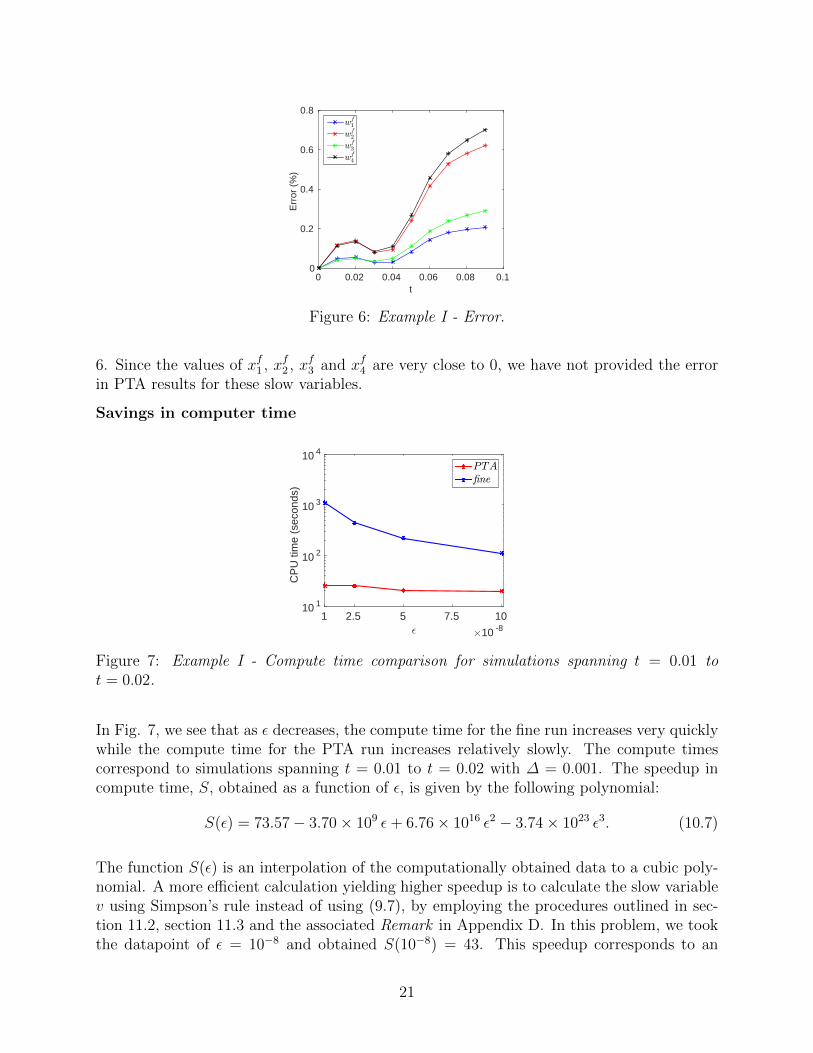
Figure 3: The rapidly oscillating solutionof the full equation of w3 is given by theplot marked w3. The drift in the fine andPTA values cannot be seen on the givenscale. But the drift is visible in Fig. 4.The PTA and the fine results overlap.

Fig. 2 shows the rapid oscillations of the rapidly oscillating variable x1 and the evolution ofthe slow variable xf1 . Fig. 3 shows the rapid oscillations of w3 and the evolution of the slowvariable wf3 . We find that x3 and x4 evolve exactly in a similar way as x1 and x2 respectively.We find from the results that xf3 , xf4 , wf3 and wf4 evolve exactly similarly as xf1 , xf2 , wf1 andwf2 respectively.

t0 0.02 0.04 0.06 0.08 0.1

0.361

0.3615

0.362

0.3625

0.363

0.3635

0.364

-nePTA

Figure 4: Evolution of wf3 .

t0 0.02 0.04 0.06 0.08 0.1

0.1365

0.137

0.1375

0.138

0.1385

0.139

0.1395-nePTA

Figure 5: Evolution of wf4 .

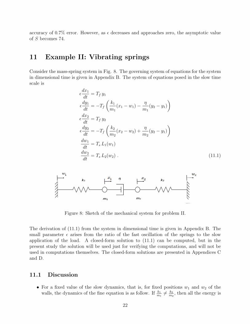
The comparison between the fine and the PTA results of the slow variables wf3 and wf4 areshown in Fig. 4 and Fig. 5 (we have not shown the evolution of wf1 and wf2 since they evolveexactly similarly to wf3 and wf4 respectively). The error in the PTA results are shown in Fig.

20

t0 0.02 0.04 0.06 0.08 0.1

Err

or (

%)

0

0.2

0.4

0.6

0.8wf

1

wf2

wf3

wf4

Figure 6: Example I - Error.

6. Since the values of xf1 , xf2 , xf3 and xf4 are very close to 0, we have not provided the errorin PTA results for these slow variables.

Savings in computer time

0 #10 -81 2.5 5 7.5 10

CP

U ti

me

(sec

onds

)

10 1

10 2

10 3

10 4

PTA-ne

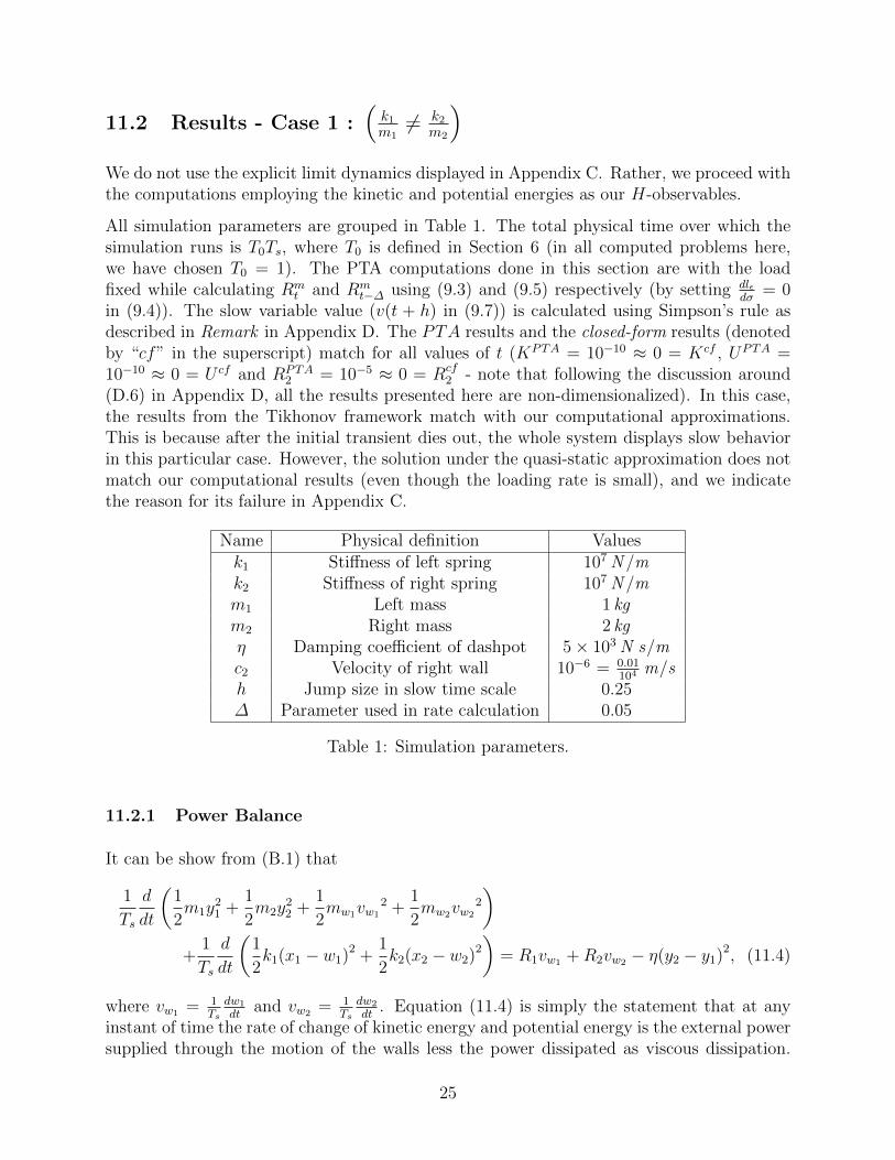
Figure 7: Example I - Compute time comparison for simulations spanning t = 0.01 tot = 0.02.

In Fig. 7, we see that as ε decreases, the compute time for the fine run increases very quicklywhile the compute time for the PTA run increases relatively slowly. The compute timescorrespond to simulations spanning t = 0.01 to t = 0.02 with ∆ = 0.001. The speedup incompute time, S, obtained as a function of ε, is given by the following polynomial:

S(ε) = 73.57− 3.70× 109 ε+ 6.76× 1016 ε2 − 3.74× 1023 ε3. (10.7)

The function S(ε) is an interpolation of the computationally obtained data to a cubic poly-nomial. A more efficient calculation yielding higher speedup is to calculate the slow variablev using Simpson’s rule instead of using (9.7), by employing the procedures outlined in sec-tion 11.2, section 11.3 and the associated Remark in Appendix D. In this problem, we tookthe datapoint of ε = 10−8 and obtained S(10−8) = 43. This speedup corresponds to an

21

accuracy of 0.7% error. However, as ε decreases and approaches zero, the asymptotic valueof S becomes 74.

11 Example II: Vibrating springs

Consider the mass-spring system in Fig. 8. The governing system of equations for the systemin dimensional time is given in Appendix B. The system of equations posed in the slow timescale is

εdx1

dt= Tf y1

εdy1

dt= −Tf

(k1

m1

(x1 − w1)− η

m1

(y2 − y1)

)εdx2

dt= Tf y2

εdy2

dt= −Tf

(k2

m2

(x2 − w2) +η

m2

(y2 − y1)

)dw1

dt= Ts L1(w1)

dw2

dt= Ts L2(w2) . (11.1)

Figure 8: Sketch of the mechanical system for problem II.

The derivation of (11.1) from the system in dimensional time is given in Appendix B. Thesmall parameter ε arises from the ratio of the fast oscillation of the springs to the slowapplication of the load. A closed-form solution to (11.1) can be computed, but in thepresent study the solution will be used just for verifying the computations, and will not beused in computations themselves. The closed-form solutions are presented in Appendices Cand D.

11.1 Discussion

• For a fixed value of the slow dynamics, that is, for fixed positions w1 and w2 of thewalls, the dynamics of the fine equation is as follow. If k1

m16= k2

m2, then all the energy is

22

dissipated, and the trajectory converges to the origin (the reason behind this behavioris explained in the Remark of Appendix C). If the equality holds, only part of theenergy possessed by the initial conditions is dissipated, and the trajectory convergesto a periodic one (in rare cases it will be the origin), whose energy is determined bythe initial condition (the reason behind this behavior is explained in Case 2.1 and Case2.2 of Section 11.3 and in the Remark of Appendix D). The computational challengeis when fast oscillations persist. Then the limiting periodic solution determines aninvariant measure for the fast flow. When the walls move, slowly, the limit invariantmeasure moves as well. The computations should detect this movement. However, ifthe walls move very slowly, there is a possibility that in the limit the energy does notchange at all as the walls move.

Notice that the invariant measure is not determined by the position of the walls, andadditional slow observables should be incorporated. A possible candidate is the totalenergy stored in the invariant measure. Since the total energy is constant on the limitcycle, it forms an orthogonal observable as described in section 4. Its extrapolation ruleis given by (5.1). In order to apply (5.1) one has to derive the effect of the movementof the walls on the observable, namely, on the total energy.

Two other observables could be the average kinetic energy and the average potentialenergy on the invariant measure. In both cases, the form of H-observables shouldbe employed, as it is not clear how to come up with an extrapolation rules for theseobservables.

It is clear that with the three observables just mentioned, if the two forcing elementsL1 and L2 in (11.1) are Lipschitz, then conditions (8.1) and (8.2) are satisfied, and,consequently, the conclusion of Theorem 8.2 holds.

• We define kinetic energy (K), potential energy (U) and reaction force on the right wall(R2) as:

K(σ) =1

2

(m1 y1,ε(σ)2 +m2 y2,ε(σ)2)

U(σ) =1

2k1(x1,ε(σ)− w1,ε(σ))2 +

1

2k2(x2,ε(σ)− w2,ε(σ))2 (11.2)

R2(σ) = −k2 (x2,ε(σ)− w2,ε(σ)) .

• The H-observables that we obtained in this example are the average kinetic energy(Kf ), average potential energy (U f ) and average reaction force on the right wall (Rf

2)

23

which are calculated as:

Kf (t) =1

N ′

N ′∑i=1

K(σi)

U f (t) =1

N ′

N ′∑i=1

U(σi) (11.3)

Rf2(t) =

1

N ′

N ′∑i=1

R2(σi),

where N ′ is defined in the discussion following (9.7) and successive values x1,ε(σi),x2,ε(σi), y1,ε(σi) and y2,ε(σi) are obtained by solving the fine system associated with(11.1) (see (B.3) in Appendix B) with appropriate initial conditions which is discussedin detail in Step 3 of Section 9. The computations are done when L1(w1) = 0 andL2(w2) = c2.

• To integrate the fine system (B.3), we use a modification of the velocity Verlet integra-tion scheme to account for damping (given in [San16]). This is done so that the energyof the system does not diverge in time due to energy errors of the numerical method.

• As we will show in Section 11.2 (where we show results for the case corresponding tothe condition k1

m16= k2

m2which we call Case 1) and Section 11.3 (where we show results

for the case corresponding to the condition k1m1

= k2m2

which we call Case 2) respectively,in Case 1, the fine evolution converges to a singleton (in the case without forcing) whilein Case 2, the fine evolution generically converges to a limit set that is not a singleton(which will be shown in Case 2.2 in Section 11.3), which shows the distinction betweenthe two cases. This has significant impact on the results of average kinetic and potentialenergy. Our computational scheme requires no a-priori knowledge of these importantdistinctions and predicts the correct approximations of the limit solution in all of thecases considered.

• For the sake of comparison with our computational approximations, in Appendix Cwe provide solutions to our system (11.1) corresponding to the Tikhonov framework[TVS85] and the quasi-static assumption commonly made in solid mechanics for me-chanical systems forced at small loading rates. We show that the quasi-static as-sumption does not apply for this problem. The Tikhonov framework applies in somesituations and our computation results are consistent with these conclusions. As acautionary note involving limit solutions (even when valid), we note that evaluatingnonlinear functions like potential and kinetic energy on the weak limit solutions as areflection of the limit of potential and kinetic energy along sequences of solutions of(11.1) as ε → 0 (or equivalently Ts → ∞) does not make sense in general, especiallywhen oscillations persist in the limit. Indeed, we observe this for all results in Case 2.

• All results shown in this section are obtained from numerical calculations, with noreference to the closed-form solutions. The closed-form solution for Case 1 is derivedin Appendix C while the closed-form solution for Case 2 is derived in Appendix D.

24

11.2 Results - Case 1 :(

k1m16= k2

m2

)We do not use the explicit limit dynamics displayed in Appendix C. Rather, we proceed withthe computations employing the kinetic and potential energies as our H-observables.

All simulation parameters are grouped in Table 1. The total physical time over which thesimulation runs is T0Ts, where T0 is defined in Section 6 (in all computed problems here,we have chosen T0 = 1). The PTA computations done in this section are with the loadfixed while calculating Rm

t and Rmt−∆ using (9.3) and (9.5) respectively (by setting dlε

dσ= 0

in (9.4)). The slow variable value (v(t + h) in (9.7)) is calculated using Simpson’s rule asdescribed in Remark in Appendix D. The PTA results and the closed-form results (denotedby “cf” in the superscript) match for all values of t (KPTA = 10−10 ≈ 0 = Kcf , UPTA =10−10 ≈ 0 = U cf and RPTA

2 = 10−5 ≈ 0 = Rcf2 - note that following the discussion around

(D.6) in Appendix D, all the results presented here are non-dimensionalized). In this case,the results from the Tikhonov framework match with our computational approximations.This is because after the initial transient dies out, the whole system displays slow behaviorin this particular case. However, the solution under the quasi-static approximation does notmatch our computational results (even though the loading rate is small), and we indicatethe reason for its failure in Appendix C.

Name Physical definition Valuesk1 Stiffness of left spring 107 N /mk2 Stiffness of right spring 107 N /mm1 Left mass 1 kgm2 Right mass 2 kgη Damping coefficient of dashpot 5× 103 N s/mc2 Velocity of right wall 10−6 = 0.01

104m/s

h Jump size in slow time scale 0.25∆ Parameter used in rate calculation 0.05

Table 1: Simulation parameters.

11.2.1 Power Balance

It can be show from (B.1) that

1

Ts

d

dt

(1

2m1y

21 +

1

2m2y

22 +

1

2mw1vw1

2 +1

2mw2vw2

2

)+

1

Ts

d

dt

(1

2k1(x1 − w1)2 +

1

2k2(x2 − w2)2

)= R1vw1 +R2vw2 − η(y2 − y1)2, (11.4)

where vw1 = 1Ts

dw1

dtand vw2 = 1

Tsdw2

dt. Equation (11.4) is simply the statement that at any

instant of time the rate of change of kinetic energy and potential energy is the external powersupplied through the motion of the walls less the power dissipated as viscous dissipation.

25

This means that the sum of the kinetic and potential energy of the system, is equal tothe sum of the initial kinetic and potential energy, plus the integral of the external powersupplied to the system, minus the viscous dissipation.

The fine solution indicates that, for c2 small, the dashpot kills all the initial potential andkinetic energy supplied to the system. The two springs get stretched based on the valueof c2. The stretches remain fixed for large times on the fast time scale and the mass m2

and the right wall move with the same velocity with mass m1 remaining fixed. Thus theright spring moves like a rigid body. Based on this argument and from (11.4), the viscous,dissipated power in the system at large fast times is ηc2

2, which is equal to the externalpower provided to the system (noting that even though mass m2 moves for large times, itdoes so with uniform velocity in this problem resulting in no contribution to the rate ofchange of kinetic energy of the system).

Savings in Computer time

0 #10 -50 0.5 1 1.5 2

CP

U ti

me

(sec

onds

)

10 2

10 3

10 4

10 5

10 6

PTA-ne

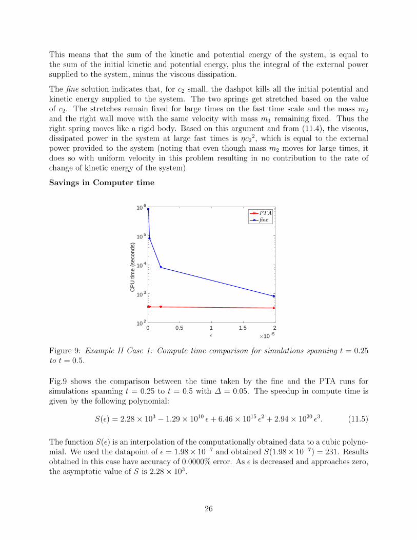
Figure 9: Example II Case 1: Compute time comparison for simulations spanning t = 0.25to t = 0.5.

Fig.9 shows the comparison between the time taken by the fine and the PTA runs forsimulations spanning t = 0.25 to t = 0.5 with ∆ = 0.05. The speedup in compute time isgiven by the following polynomial:

S(ε) = 2.28× 103 − 1.29× 1010 ε+ 6.46× 1015 ε2 + 2.94× 1020 ε3. (11.5)

The function S(ε) is an interpolation of the computationally obtained data to a cubic polyno-mial. We used the datapoint of ε = 1.98× 10−7 and obtained S(1.98× 10−7) = 231. Resultsobtained in this case have accuracy of 0.0000% error. As ε is decreased and approaches zero,the asymptotic value of S is 2.28× 103.

26

11.3 Results - Case 2:(

k1m1

= k2m2

)As already noted, in this case the quasi-static approach is not valid. The closed-form solutionto this case is displayed in Appendix D (but it is not used in the computations). Recall thatthe computations are carried out when L1(w1) = 0 and L2(w2) = c2. The PTA computationsdone in this section are with the load fixed while calculating Rm

t and Rmt−∆ using (9.3) and

(9.5) respectively (by setting dlεdσ

= 0 in (9.4)). The slow variable value (v(t+ h) in (9.7)) iscalculated using Simpson’s rule as described in Remark in Appendix D. All results in thissection are non-dimensionalized following the discussion around (D.6) in Appendix D.

The following cases arise:

• Case 2.1. When c2 = 0 and the initial condition does not have a component onthe modes describing the dashpot being undeformed (x1 = x2 and y1 = y2), then thesolution will go to rest. For example, the initial conditions x1

0 = 1.0, x20 = −0.5 and

y10 = y2

0 = 0.0 makes the solution (D.4) of Appendix D go to rest (κ3 = κ4 = 0 in(D.9) of Appendix D). The simulation results agree with the closed-form results andgo to zero.

• Case 2.2. When c2 = 0 and the initial condition has a component on the modesdescribing the dashpot being undeformed, then in the fast time limit the solutionshows periodic oscillations whose energy is determined by the initial conditions. Thishappens, of course, for almost all initial conditions. One such initial condition isx1

0 = 0.5, x20 = −0.1 and y1

0 = y20 = 0 (κ3 = 0 but κ4 = −0.4472 in (D.9) of

Appendix D). The simulation results agree with the closed-form results.

This is in contrast with Case 1 where it is impossible to find initial conditions for whichthe solution shows periodic oscillations.

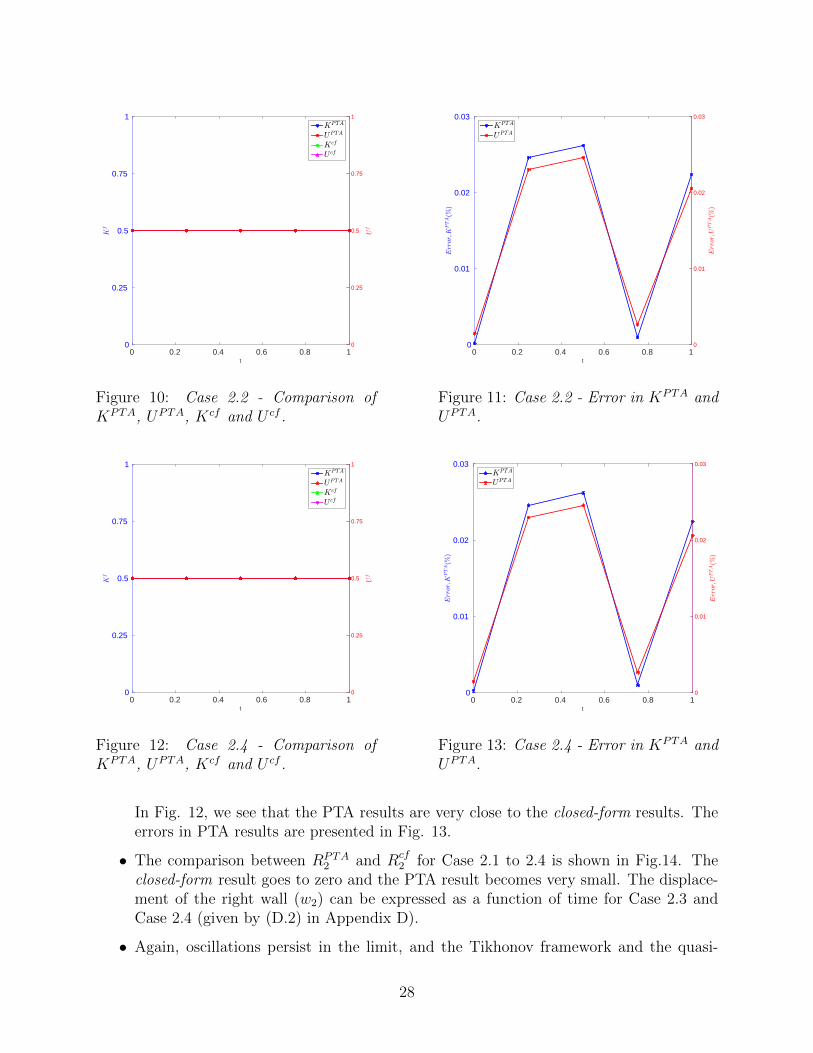
In Fig. 10, we see that the PTA results are very close to the closed-form results. Theerror in PTA results are presented in Fig. 11.

Oscillations persist in the limit and the potential and kinetic energies computed basedon the Tikhonov framework as well as the quasi-static solution (C.6) derived in Ap-pendix C are not expected to, and do not, yield correct answers.

• Case 2.3. When c2 6= 0 and the initial condition does not have a component on themodes describing the dashpot being undeformed, then the solution on the fast timescale for large values of σ does not depend on the initial condition. One such initialcondition is x1

0 = 1.0, x20 = −0.5 and y1

0 = 0.0 and y20 = 10−4. The closed-form

average kinetic energy (Kcf ) and closed-form average potential energy (U cf ) do notdepend on the magnitude of the initial conditions in this case.

• Case 2.4. The initial condition has a component on the modes describing the dashpotbeing undeformed. But when c2 6= 0, the dashpot gets deformed due to the translationof the mass m2. The closed-form average kinetic energy (Kcf ) and closed-form averagepotential energy (U cf ) depend on the initial conditions.

27

t0 0.2 0.4 0.6 0.8 1

Kf

0

0.25

0.5

0.75

1

Uf

0

0.25

0.5

0.75

1

KPTA

UPTA

Kcf

U cf

Figure 10: Case 2.2 - Comparison ofKPTA, UPTA, Kcf and U cf .

t0 0.2 0.4 0.6 0.8 1

Err

or;K

PTA(%

)

0

0.01

0.02

0.03

Err

or;U

PTA(%

)

0

0.01

0.02

0.03

KPTA

UPTA

Figure 11: Case 2.2 - Error in KPTA andUPTA.

t0 0.2 0.4 0.6 0.8 1

Kf

0

0.25

0.5

0.75

1

Uf

0

0.25

0.5

0.75

1

KPTA

UPTA

Kcf

U cf

Figure 12: Case 2.4 - Comparison ofKPTA, UPTA, Kcf and U cf .

t0 0.2 0.4 0.6 0.8 1

Err

or;K

PTA(%

)

0

0.01

0.02

0.03

Err

or;U

PTA(%

)

0

0.01

0.02

0.03

KPTA

UPTA

Figure 13: Case 2.4 - Error in KPTA andUPTA.

In Fig. 12, we see that the PTA results are very close to the closed-form results. Theerrors in PTA results are presented in Fig. 13.

• The comparison between RPTA2 and Rcf

2 for Case 2.1 to 2.4 is shown in Fig.14. Theclosed-form result goes to zero and the PTA result becomes very small. The displace-ment of the right wall (w2) can be expressed as a function of time for Case 2.3 andCase 2.4 (given by (D.2) in Appendix D).

• Again, oscillations persist in the limit, and the Tikhonov framework and the quasi-

28

static approximation (see Appendix C) do not work in this case.

• The results do not change if we decrease the value of ε. However, the speedup changesas will be shown in Savings in Computer time later in this section.

t0 0.2 0.4 0.6 0.8 1

#10 -4

-6

-4

-2

0

2

4

6

RPTA2 !Case 2:1

RPTA2 !Case 2:2

RPTA2 !Case 2:3

RPTA2 !Case 2:4

Rcf2

Figure 14: Case 2.1 to 2.4: Comparison of RPTA2 and Rcf

2 .

We used the same simulation parameters as in Case 1 ( shown in Table 1 ) but with k2 = 2×107N/m so that k1

m1= k2

m2. Let us assume that the strain rate is 10−4s−1. Then the slow time

period, Ts = 1˙ε

= 10000s. The fast time period is obtained as the period of fast oscillations

of the spring, given by, Tf = 2π√

m1

k1= 0.002s. Thus, we find ε =

TfTs

= 1.98× 10−7. While

running the PTA code with ε = 0.002, we have seen that the PTA scheme is not able to giveaccurate results and it breaks down.

Power BalanceThe input power supplied to the system is 1

TsR2

dw2

dt. Since R2 = k2(w2−x2) and dw2

dt= Ts c2,

the average value of input power at time t is 1∆

∫ t+∆t

k2(w2−x2)c2 dt′. From the results in (D.4)

of Appendix D and noting that the average of oscillatory terms over time ∆ is approximately0, we see that 1

∆

∫ t+∆t

(w2 − x2) dt′ = 1∆

∫ t+∆t{c2Tst

′−(c2Tst′− ηc2

k2)} dt′ = ηc2

k2. Hence average

input power supplied is ηc22. The average dissipation at time t is 1

∆

∫ t+∆t

ηT 2s

(dx2dt′− dx1

dt′)2dt′.

Using the result from (D.4) of Appendix D, and using the same argument that the averageof oscillatory terms over time ∆ is approximately 0, we can say that the dissipation is ηc2

2.Thus, the average input power supplied to the system is equal to the dissipation in thedamper. A part of the input power also goes into the translation of the mass m2. But itsvalue is very small compared to the total kinetic energy of the system.

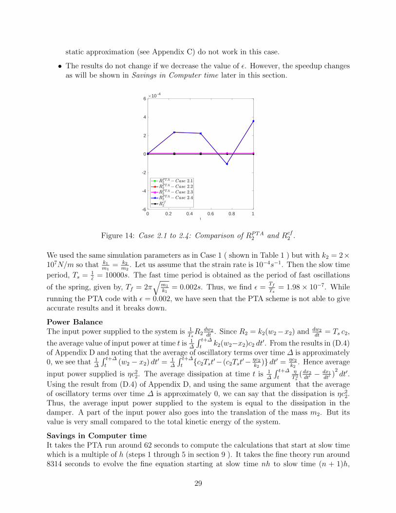
Savings in Computer timeIt takes the PTA run around 62 seconds to compute the calculations that start at slow timewhich is a multiple of h (steps 1 through 5 in section 9 ). It takes the fine theory run around8314 seconds to evolve the fine equation starting at slow time nh to slow time (n + 1)h,

29

where n is a positive integer. Thus, we could achieve a speedup of 134. We expect that thespeedup will increase if we decrease the value of ε.

0 #10 -50 0.5 1 1.5 2

CP

U ti

me

(sec

onds

)

10 1

10 2

10 3

10 4

PTA-ne

Figure 15: Example II Case 2: Compute time comparison for simulations spanning t = 0.25to t = 0.5.

Fig.15 shows the comparison between the time taken by the fine and the PTA runs forsimulations spanning t = 0.25 to t = 0.5 with ∆ = 0.05.

The speedup in compute time is given by the following polynomial:

S(ε) = 164.34− 1.62× 108 ε+ 5.23× 1013 ε2 − 2.25× 1018ε3. (11.6)

The function S(ε) is an interpolation of the computationally obtained data to a cubic poly-nomial. We used the datapoint of ε = 1.98× 10−7 and obtained S(1.98× 10−7) = 134. Thisspeedup corresponds to an accuracy of 0.026% error. As ε is decreased and approaches zero,the asymptotic value of S is 164.

12 Example III: Relaxation oscillations of oscillators

This is a variation of the classical relaxation oscillation example(see, e.g., [Art02]). Considerthe four-dimensional system

dx

dt= z

dy

dt=

1

ε(−x+ y − y3) (12.1)

dz

dt=

1

ε(w + (z − y)(

1

8− w2 − (z − y)2))

dw

dt=

1

ε(−(z − y) + w(

1

8− w2 − (z − y)2)).

30

Notice that the (z, w) coordinates oscillate around the point (y, 0) (in the (z, w)-space),with oscillations that converge to a circular limit cycle of radius 1√

8. The coordinates (x, y)

follow the classical relaxation oscillations pattern (for the fun of it, we replaced y in theslow equation by z, whose average in the limit is y). In particular, the limit dynamics ofthe y-coordinate moves slowly along the stable branches of the curve 0 = −x+ y − y3, withdiscontinuities at x = − 2

3√

3and x = 2

3√

3. In turn, these discontinuities carry with them

discontinuities of the oscillations in the (z, w) coordinates. The goal of the computation isto follow the limit behavior, including the discontinuities of the oscillations.

12.1 Discussion

The slow dynamics, or the load, in the example is the x-variable. Its value does not determinethe limit invariant measure in the fast dynamics, which comprises a point y and a limitcircle in the (z, w)-coordinates. A slow observable that will determine the limit invariantmeasure is the y-coordinate. In particular, conditions (8.1) an (8.2) hold except at pointsof discontinuity, and so does the conclusion of Theorem 8.2. Notice, however, that thisobservable does go through periodic discontinuities.

12.2 Results

We see in Fig. 16 that the y-coordinate moves slowly along the stable branches of the curve0 = −x + y − y3 which is evident from the high density of points in these branches of thecurve as can be seen in Fig. 16. There are also two discontinuities at x = − 2

3√

3and x = 2

3√

3.

The pair (z, w) oscillates around (y, 0) in circular limit cycle of radius 1√8.

In Fig. 17, we see that the average of z and y which are given by the y-coordinate in theplot, are the same which acts as a verification that our scheme works correctly. Also, averageof w is 0 as expected.

Since there is a jump in the evolution of the measure at the discontinuities (of the Youngmeasure), the observable value obtained using extrapolation rule is not able to follow thisjump. However, the observable values obtained using the guess for fine initial conditions atthe next jump could follow the discontinuity. This is the principal computational demon-stration of this example.

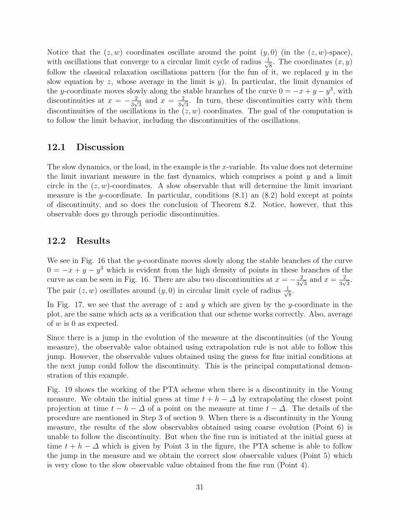
Fig. 19 shows the working of the PTA scheme when there is a discontinuity in the Youngmeasure. We obtain the initial guess at time t + h − ∆ by extrapolating the closest pointprojection at time t − h − ∆ of a point on the measure at time t − ∆. The details of theprocedure are mentioned in Step 3 of section 9. When there is a discontinuity in the Youngmeasure, the results of the slow observables obtained using coarse evolution (Point 6) isunable to follow the discontinuity. But when the fine run is initiated at the initial guess attime t + h − ∆ which is given by Point 3 in the figure, the PTA scheme is able to followthe jump in the measure and we obtain the correct slow observable values (Point 5) whichis very close to the slow observable value obtained from the fine run (Point 4).

31

t2

t1

t1<t2

Figure 16: Trajectory of (12.1). The ver-tical branches of the y vs x curve corre-spond to very fast move on the fast timescale. The blue curve shows the portionof the phase portrait of the z vs w tra-jectory obtained around time t1 while thebrown curve shows the portion around alater time t2. (For interpretation of thereferences to color in this figure legend,the reader is referred to the web versionof this article.)

Figure 17: PTA result. The portion with thearrows correspond to very rapid evolution onthe slow time scale.

0

10 -10 10 -9 10 -8 10 -7

CP

U ti

me

(sec

onds

)

10 1

10 2

10 3

10 4

10 5

PTA-ne

Figure 18: Example III - Compute time comparison for simulations spanning t = 0.2 tot = 0.4.

32

x-1 -0.5 0 0.5 1 1.5

y

-1.5

-1

-0.5

0

0.5

1

1.5

yPTA vs xPTA

curve 1point 1curve 2point 2curve 3point 3point 4point5point6

(a)

w-1 -0.5 0 0.5 1 1.5

z

-2

-1.5

-1

-0.5

0

0.5

1

1.5

zPTA vs wPTA

curve 1point 1curve 2point 2curve 3point 3point 4point 5point 6

(b)

Figure 19: This figure shows how PTA scheme predicts the correct values of slow observableswhen there is a discontinuity in the Young measure. Part (a) shows the details for y vs x.The denotations of the different points mentioned here are provided in Step 3 of Section 9.Curve 1 is the set of all points in support of the measure at time t−h−∆. The point xcpt−h−∆is given by point 1 in the figure (we obtain Curve 1 and point 1 using the details mentionedin Step 3 of Section 9). Curve 1 reduces to a point near point 1, so it is not visible in thefigure. Curve 2 is the set of all points in support of the measure at time t − ∆. The pointxarbt−∆ is given by point 2 (we obtain Curve 2 and point 2 using the details mentioned in Step3 of Section 9). Curve 2 reduces to a point very close to point 2, so it is not visible. Point 3is the initial guess for time t+h−∆ which we calculate using the details in Step 3 of Section9. Curve 3 is the set of all points in support of the measure at time t + h − ∆. The slowobservable value at time t+ h−∆ obtained from the fine run is point 4. Point 5 is the slowobservable value obtained from the PTA run using the details in Step 4 of Section 9. Point 6corresponds to slow observable values obtained solely by using the coarse evolution equationwithout using the initial guess at time t+ h−∆ (using Step 2 of Section 9). Part (b) showsthe corresponding details for z vsw. In this figure, we see that Curve 1 and Curve 2 do notreduce to a point.

Savings in computer time. Fig.18 shows the comparison between the time taken bythe fine and the PTA runs for simulations spanning t = 0.2 to t = 0.4 with ∆ = 0.01.The speedup in compute time as a function of ε for ∆ = 0.01, is given by the followingpolynomial:

S(ε) = 1.29× 103 − 1.19× 1012 ε+ 1.17× 1020 ε2 − 1.05× 1027 ε3. (12.2)

The function S(ε) is an interpolation of the computationally obtained data to a cubic poly-nomial. A more efficient calculation yielding higher speedup is to calculate the slow variablev using Simpson’s rule instead of using (9.7), by employing the procedures outlined in sec-

33

tion 11.2, section 11.3 and the associated Remark in Appendix D. We used the datapoint ofε = 10−10 for this problem and obtained S(10−10) = 1.17×103. This speedup corresponds toan accuracy of 4.33% error. As we further decrease ε and it approaches zero, the asymptoticvalue of S becomes 1.29× 103.

Remark. As a practical matter, it seems advantageous to set ε = 0 in (9.4) for the compu-tations of Rm

t−∆ in (9.5) and Rmt in (9.3). Related to this, when the value of ε is decreased,

calculating the slow variable value (v(t + h) in (9.7)) using Simpson’s rule as described inRemark in Appendix D reduces T cpuPTA considerably and improves the speedup S(ε).

13 Concluding remarks

The focus of this paper has been the precise definition and demonstration of a computationaltool to probe slow time-scale behavior of rapidly evolving microscopic dynamics, whetheroscillatory or exponentially decaying to a manifold of slow variables, or containing bothbehaviors. A prime novelty of our approach is in the introduction of a general family of ob-servables (H-observables) that is universally available, and a practical computational schemethat covers cases where the invariant measures may not be uniquely determined by the slowvariables in play, and one that allows the tracking of slow dynamics even at points of dis-continuity of the Young measure. We have solved three model problems that neverthelesscontain most of the complications of averaging complex multiscale temporal dynamics. Itcan be hoped that the developed tool is of substantial generality for attacking real-worldpractical problems related to understanding and engineering complex microscopic dynamicsin relatively simpler terms.

34

Appendix A Verlet Integration

The implementation of Verlet scheme that we used in Example II to integrate the fineequation (B.3) is as follows [San16]:

x1(σ +∆σ) = x1(σ) +∆σ y1(σ) +1

2∆σ2 dy1

dσ

x2(σ +∆σ) = x2(σ) +∆σ y2(σ) +1

2∆σ2 dy2

dσ

y1(σ +∆σ) = y1(σ) +1

2∆σ

(dy1

dσ+ a1

{x1(σ +∆σ), y1(σ) +∆σ

dy1

dσ, y2(σ) +∆σ

dy2

dσ, w1(σ)

})y2(σ +∆σ) = y2(σ) +

1

2∆σ

(dy2

dσ+ a2

{x2(σ +∆σ), y1(σ) +∆σ

dy1

dσ, y2(σ) +∆σ

dy2

dσ, w2(σ)

})y1(σ +∆σ) = y1(σ) +

1

2∆σ

(dy1

dσ+ a1 {x1(σ +∆σ), y1(σ +∆σ), y2(σ +∆σ), w1(σ)}

)y2(σ +∆σ) = y2(σ) +

1

2∆σ

(dy2

dσ+ a2 {x2(σ +∆σ), y1(σ +∆σ), y2(σ +∆σ), w2(σ)}

).

(A.1)

Here a1(x1, y1, y2, w1) = dy1dσ

and a2(x2, y1, y2, w2) = dy2dσ

where dy1dσ

and dy2dσ

are given by(B.3).

Appendix B Example II: Derivation of system of equa-

tions

Two massless springs and masses m1 and m2 are connected through a dashpot damper, andeach is attached to two bars, or walls, that may move very slowly, compared to possibleoscillations of the springs. The system is described in Fig. 8 of Section 11.

Let the springs constants be k1 and k2 respectively, and let η be the dashpot constant.Denote by x1 and x2, and by w1 and w2, the displacements from equilibrium positions ofthe masses of the springs and the positions of the two walls. We agree here that all positivedisplacements are toward the right. We think of the movement of the two walls as beingexternal to the system, determined by a “slow” differential equation. The movement of thesprings, however, will be “fast”, which we model as singularly perturbed. Let mw1 and mw2

be the masses of the left and the right walls respectively. The displacements x1, x2, w1

and w2 have physical dimensions of length. The spring constants k1 and k2 have physicaldimensions of force per unit length while m1 and m2 have physical dimensions of mass. Inview of the assumptions just made, a general form of the dynamics of the system is given by

35

following set of equations:

m1d2x1

dt∗2= −k1(x1 − w1) + η

(dx2

dt∗− dx1

dt∗

)m2

d2x2

dt∗2= −k2(x2 − w2)− η

(dx2

dt∗− dx1

dt∗

)(B.1)

mw1

d2w1

dt∗2= k1(x1 − w1) +R1

mw2

d2w2

dt∗2= k2(x2 − w2) +R2,

where R1 and R2 incorporate the reaction forces on the left and right walls respectivelydue to their prescribed motion. We agree that forces acting toward the right are beingconsidered positive. We make the assumption that mw1 = mw2 = 0. The time scale t∗ isa time scale with physical dimensions of time. In our calculations, however, we address asimplified version, of first order equations, that can be obtained from the previous set byappropriately specifying what the forces on the system are:

dx1

dt∗= y1

dy1

dt∗= − k1

m1

(x1 − w1) +η

m1

(y2 − y1)

dx2

dt∗= y2 (B.2)

dy2

dt∗= − k2

m2

(x2 − w2)− η

m2

(y2 − y1)

dw1

dt∗= L1(w1)

dw2

dt∗= L2(w2).

The motion of the walls are determined by the functions L1(w1) and L2(w2). In the deriva-tions that follow, we use the form L1(w1) = c1 and L2(w2) = c2, with c1 = 0 and c2 being aconstant. The terms c1 and c2 have physical dimensions of velocity.

We define a coarse time period, Ts, in terms of the applied loading rate as Ts = constL2

. Hence,Tsc2 is a constant which is independent of the value of Ts. The fine time period, Tf , isdefined as the smaller of the periods of the two spring mass systems. We then define thenon-dimensional slow and fast time scales as t = t∗

Tsand σ = t∗

Tf, respectively. The parameter

ε is given by ε =TfTs

. Then the dynamics on the slow time-scale is given by (11.1) in Section11. The dynamics on the fast time-scale is written as:

36

dx1

dσ= Tf y1

dy1

dσ= −Tf

(k1

m1

(x1 − w1)− η

m1

(y2 − y1)

)dx2

dσ= Tf y2

dy2

dσ= −Tf

(k2

m2

(x2 − w2) +η

m2

(y2 − y1)

)dw1

dσ= ε Ts L1(w1)

dw2

dσ= ε Ts L2(w2). (B.3)

Remark. A special case of (11.1) is when c1 = 0 and c2 = 0. This represents the unforcedsystem i.e. the walls remain fixed. Then (11.1) is modified to:

x = Bx, (B.4)

where x = (x1, y1, x2, y2)T . The overhead dot represent time derivatives w.r.t. t. The matrixB is given by

B = Ts

0 1 0 0− k1m1− ηm1

0 ηm1

0 0 0 10 η

m2− k2m2− ηm2

.

Appendix C Example II: Case 1 - Validity of com-

monly used approximations

The mechanical system (11.1) can be written in the form(TiTs

)2

A1d2x

dt2+

(TνTs

)A2

dx

dt+ A3x =

F

k(C.1)

dw

dt= L(w),

where t = t∗

Tswhere t∗ is dimensional time and Ts is a time-scale of loading defined below,

Ti2 = m

k, Tν = D

k(the mass m, damping D and stiffness k have physical dimensions of

mass, Force×timelength

and ForceLength

respectively), x and w are displacements with physical unitsof length, L is a function, independent of Ts, with physical units of length , and A1, A2

and A3 are non-dimensional matrices. In this notation, TiTs

= ε. In the examples considered,L = c = Tsc, where c has physical dimensions of velocity and is assumed given in the formc = c

Tsthus serving to define Ts; c has dimensions of length.

37

Necessary conditions for the application of the Tikhonov framework are that TiTs→ 0, Tν

Ts→ 0

as Ts →∞. Those for the quasi-static assumption, commonly used in solid mechanics whenloading rates are small, are that Ti

Ts→ 0 and Tν

Ts≈ 1 as Ts →∞.

In our example, we have m = 1kg,k = 2 × 107N/m, D = 5 × 103Ns/m and Ts = 100s.Hence Ti

Ts= 2.24× 10−6 and Tν

Ts= 2.5× 10−6, and the damping is not envisaged as variable

as Ts →∞, which shows that the quasi-static approximation is not applicable.

Nevertheless, due to the common use of the quasi-assumption under slow loading in solidmechanics (which amounts to setting εdy1

dt= 0, εdy2

dt= 0 in (11.1)), we record the quasi-static

solution as well.

The Tikhonov framework. It is easy to see that under the conditions in Case 1, whenthe walls do not move, all solutions tend to an equilibrium (that may depend on the positionof the walls). Indeed, the only way the energy will not be dissipated is when y1(t) = y2(t)along time intervals, a not sustainable situation. Thus, we are in the classical Tikhonovframework, and, as we already noted toward the end of the introduction to the paper, thelimit solution will be of the form of steady-state equilibrium of the springs, moving on themanifold of equilibria determined by the load, namely the walls. Computing the equilibriain (11.1) (equivalently (B.2)) is straightforward. Indeed, for fixed (w1,w2) we get

x1 = w1, x2 = w2

y1 = 0, y2 = 0. (C.2)

Under the assumption that L1 = 0 and L2 = c2 we get

w1(t) = 0

w2(t) = c2Tst. (C.3)

Plugging the dynamics (C.3) in (C.2) yields the limit dynamics of the springs. The realworld approximation for ε small would be a fast movement toward the equilibrium set (i.e.,a boundary layer which has damped oscillations), then an approximation of (C.2)-(C.3).Our computations in Section 11.2 corroborate this claim.

Solutions to (11.1) seem to suggest that this is one example where the limit solution (C.2)-(C.3) is attained by a sequence of solutions of (11.1) as ε → 0 or Ts → ∞ in a ‘strong’sense (i.e. not in the ‘weak’ sense of averages); e.g. for small ε > 0, y2 takes the value c2

in the numerical calculations and this, when measured in units of slow time-scale Ts (notethat y has physical dimensions of velocity), yields Tsc2 which equals the value of the (non-dimensional) time rates of w2 and x2 corresponding to the limit solution (C.2)-(C.3); ofcourse, c2 → 0 as Ts → ∞, by definition, and therefore y2 → 0 as well. Thus, the kineticenergy and potential energy evaluated from the limit solution (C.2)-(C.3), i.e. 0 respectively,are a good approximation of the corresponding values from the actual solution for a specificvalue of small ε > 0, as given in Sec. 11.2.

38

The quasi-static assumption. We solve the system of equations:

−k1(x1 − w1) + η(y2 − y1) = 0

−k2(x2 − w2)− η(y2 − y1) = 0

y1 =1

Ts

dx1

dt

y2 =1

Ts

dx2

dt. (C.4)

We assume the left wall to be fixed and the right wall to be moving at a constant velocityof magnitude c2, so that w1 = 0 and w2 = c2 Ts t. This results in

dx1

dt+

k1Ts

η(1 + k1k2

)x1 =

c2Ts

1 + k1k2

. (C.5)

Solving for x1 and using (C.4), we get the following solution

x1 =c2η

k1

+ α e−βTst, y1 = −αβe−βTst,

x2 = c2Tst−c2η

k2

− k1

k2

αe−βTst, y2 = c2 −k1

k2

αβe−βTst, (C.6)

where α is a constant of integration and β = k1η(1+

k1k2

).

Remark. The solution of the unforced system given by (B.4) in Appendix B is of theform

x(t) =4∑i=1

QieλitVi, (C.7)

where λi and Vi are the eigenvalues and eigenvectors of B respectively. Using the valuesprovided in Table 1 to construct B, we find that λi and Vi are complex. The generalreal-valued solution to the system can be written as

∑4i=1 ψie

γitMi(t) where

ξ = 2.58× 105 j = 1 j = 2 j = 3 j = 4γj −6.17× 105 −1.22× 105 −5.63× 103 −5.63× 103

M1,j(t) 0.0001 −0.8732 −0.0001 0.4873M2,j(t) 0.0006 −0.7486 −0.0005 0.6630M3,j(t) −0.0001 cos(ξt)− 0.0003 sin(ξt) −0.6812 cos(ξt) + 0.1818 sin(ξt) −0.0003 sin(ξt) −0.7092 cos(ξt)M4,j(t) 0.0003 cos(ξt)− 0.0001 sin(ξt) −0.1818 cos(ξt) + 0.6812 sin(ξt) 0.0003 cos(ξt) −0.7092 sin(ξt)

We see that all the real (time-dependent) modes Mi(t) are decaying. Moreover, none of themodes describe the dashpot as being undeformed i.e. Mi,1(t) = Mi,3(t) and Mi,2(t) = Mi,4(t)(where Mi,j(t) is the jth row of the mode Mi(t)). Therefore, solution x(t) goes to rest whent becomes large and the initial transient dies.

39

Appendix D Example II: Case 2 - Closed-form Solu-

tion

We can convert (11.1) to the following:(x1

x2

)+ αTs

2

(x1

x2

)+ Ts

( ηm1

− ηm1

− ηm2

ηm2

)(x1

x2

)=

(αw1

αw2

), (D.1)

where α = k1m1

= k2m2

and w1 and w2 are defined as :

w1(t) = 0

w2(t) = c2 Ts t. (D.2)

The overhead dots represent time derivatives w.r.t. t. The above equation is of the form:

x + αTs2 x + TsAx = g(t), (D.3)

with the general solution

x1 = C1cos(√αTst) + C2sin(

√αTst)−

m2

m1

C3e−p1Tst − m2

m1

C4e−p2Tst +

ηc2

k1

, (D.4a)

x2 = C1cos(√αTst) + C2sin(

√αTst) + C3e

−p1Tst + C4e−p2Tst + c2 Ts t−

ηc2

k2

, (D.4b)

where p1 =η(m1+m2)+

√η2(m1+m2)2−4αm2

1m22

2m1m2and p2 =

η(m1+m2)−√η2(m1+m2)2−4αm2

1m22

2m1m2. In the

computational results in Section 11.2 and 11.3, we found that p1, p2 > 0.

Imposing initial conditions x10 and x2

0 on displacement and v10 and v2

0 on velocity of thetwo masses m1 and m2 respectively, we obtain

C1m1x10+m2x20

m1+m2

C2m1v10+m2v20−c2m2√

α(m1+m2)

C3c2ηm1p2+c2ηm2p2−αc2m1m2−αm1m2p2x10+αm1m2p2x20

αm2(m1+m2)(p1−p2)

C4c2ηm1p1+c2ηm2p1−αc2m1m2−αm1m2p1x10+αm1m2p1x20

αm2(m1+m2)(p1−p2)

The closed-form average kinetic energy (Kcf ), closed-form average potential energy (P cf )andclosed-form average reaction force (Rcf

2 ) are

Kcf (t) =1

∆

∫ t

t−∆

(1

2m1y1(s)2 +

1

2m2y2(s)2

)ds

P cf (t) =1

∆

∫ t

t−∆

(1

2k1x1(s)2 +

1

2k2 (x2(s)− w2(s))2

)ds (D.5)

Rcf2 (t) =

1

∆

∫ t

t−∆(−k2 ((x2(s)− w2(s))) ds,

40

where x1(s) and x2(s) can be substituted from (D.4) and y1(s) = 1Ts

dx1ds

and y2(s) =1sdx2ds

.

Non-dimensionalization. Let us denote

mmax = maxi

m(xε(σi), lε(σi)),

where m(xε(σi), lε(σi)) is given in (9.3) and (9.5). Please note that i is chosen such thatthere is no effect of the initial transient. Using (11.2) and computational results in Case 2.4in Section 11.3, we find that

Kmax =1

2C2

1(k1 + k2), Pmax =1

2C2

1(k1 + k2), R2,max = C1k2.

We introduce the following non-dimensional variables:

Kcf =Kcf

Kmax

, P cf =P cf

Pmax, R2

cf=

Rcf2

R2,max

. (D.6)

Henceforth, while referring to the dimensionless variables, we drop the overhead tilde forsimplicity.

t0 0.2 0.4 0.6 0.8 1

Kcf

0.4995

0.5

0.5005

0.501

0.5015

0.502

0.5025

0.503

0.5035

0.504

0.50450 = 1:98# 10!5

0 = 1:98# 10!6

0 = 1:98# 10!7

Figure 20: Kcf as a function of t.

t0 0.2 0.4 0.6 0.8 1

Pcf

0.4998

0.5

0.5002

0.5004

0.5006

0.5008

0.501

0.5012

0.50140 = 1:98# 10!5

0 = 1:98# 10!6

0 = 1:98# 10!7

Figure 21: P cf as a function of t.

We evaluated (D.5) numerically (since the analytical expressions become lengthy) with 2×106

integration points over the interval [t−∆, t] using Simpson’s rule and we used 2000 discretepoints for t. We substituted the values provided in Table 1. We repeated the calculationswith 4× 106 integration points over the interval [t−∆, t] and 4000 discrete points for t, andfound the results to be the same. We see in Fig. 20 and Fig.21 that Kcf and P cf oscillatearound 0.5 with very small amplitude for different values of ε (recall that ε =

TfTs

and we thinkof Tf being fixed with Ts →∞ to effect ε→ 0). However, as we decrease ε, the amplitude of

41

t0 0.2 0.4 0.6 0.8 1

Rcf 2

#10 -4

-1.5

-1

-0.5

0

0.5

1

1.5

2

2.5

3

3.50 = 1:98# 10!5

0 = 1:98# 10!6

0 = 1:98# 10!7

Figure 22: Rcf2 as a function of t.

oscillations of Rcf2 decreases and it goes to zero for ε = 1.98× 10−7 as we see in Fig. 22. We

use these ‘closed-form’ results to compare with the PTA results in Section 11.2 and Section11.3.

Remark. The criteria for convergence of Rmt (as mentioned in the discussion following (9.4)

in Section 9) is discussed as follows. Let us denote

mI,t =1

I

I∑i=1

m(xε(σi), lε(σi)),

where xε(σi), lε(σi) is defined in (9.4), I ∈ Z+ and m(xε(σi), lε(σi)) is non-dimensionalized∀i ∈ [1, I]. Then, we say that mI,t has converged if

|mI−jk,t − mI−pk,t

mI−pk,t| ≤ tolm1 , (D.7)

∀j ∈ [0, p] where p, k ∈ Z+ and p, k < I and tolm1 is a specified value of tolerance (whichis a small value generally around 10−2). We declare Nt = I (where Nt is defined in thediscussion following (9.4)) and Rm

t = mI,t. In situations where mI−pk,t becomes very smallso that the convergence criteria in (D.7) cannot be practically implemented, we say that mI,t

has converged if

|mI−jk,t| ≤ tolm2 , (D.8)

∀j ∈ [0, p] and tolm2 is a specified value of tolerance (generally around 10−5).

42

Remark. We used the Simpson’s rule of numerical integration to obtain the value of theslow variable instead of using (9.7) to obtain the results in Section 11.2 and 11.3. TheSimpson’s rule of numerical integration for any function f(t) over the interval [a, b] wherea, b ∈ R is∫ b

a

f(t)dt ≈ ∆t

n[f(t0) + 4f(t1) + 2f(t2) + ...+ 2f(tn−2) + 4f(tn−1) + f(tn)],

where ∆t = b−an

, n ∈ Z+, n is even and ti = t0 + i∆t for i ∈ Z and i ≤ n. All the functionevaluations at points with odd subscripts are multiplied by 4 and all the function evaluationsat points with even subscripts (except for the first and last) are multiplied by 2. Since we arecalculating the value of the slow variable v given by (9.1), the function f(t) is given by Rm

t

which is defined in (9.3), with ε = 0 in (9.4). We chose n = 2 and calculated the values ofRmt−∆+ i

n∆

using (9.3) for i = 0, 1, 2. We obtained the fine initial conditions xguess(t−∆+ in∆)

as

xguess(t−∆+i

n∆) = xarbt−∆ +

(xarbt−∆ − x

cpt−h)

(h−∆)

i∆

n,

where xarb. and xcp. are defined in Step 3 in Section 9.

Please note that we also used Simpson’s rule to evaluate (D.5) with n = 2×106 and the detailsof the calculation are mentioned in Non-dimensionalization in this Appendix above.

Remark. To see the effect of the initial condition on the solution, we solve (B.4) in a par-ticular case using the values provided in Table 1 but with k2 = 2× 107N/m and c2 = 0. Thegeneral real-valued solution to the system can be written as

∑4i=1 ψie

γitMi(t) where

ω = 3.16× 105 j = 1 j = 2 j = 3 j = 4γj −5.76× 105 −1.73× 105 0 0

M1,j(t) 0.0002 −0.8944 −0.0001 0.4472M2,j(t) 0.0005 −0.8944 −0.0003 0.4421M3,j(t) 0.0002 sin(ωt) −0.7071 cos(ωt) 0.0002 sin(ωt) 0.7071 cos(ωt)M4,j(t) −0.0002 cos(ωt) 0.7071 sin(ωt) −0.0002 cos(ωt) 0.7071 sin(ωt)

We see that while M1(t) and M2(t) are decaying real (time-dependent) modes, M3(t) andM4(t) are the non-decaying real (time-dependent) modes. Moreover, both M3(t) and M4(t)describe the dashpot as being undeformed i.e. Mi,1(t) = Mi,3(t) and Mi,2(t) = Mi,4(t)(where Mi,j(t) is the jth row of the mode Mi(t)). The solution x(t) described in (C.7) ofAppendix C can be written as

x(t) =4∑i=1

κiMi(t), (D.9)

where the coefficients κi are obtained from the initial condition x0 using

κi = x0 ·Mdi (0)

where Mdi (t) are the dual basis of Mi(t).

43

Acknowledgment

We thank the anonymous referees for their valuable comments that helped improve the pre-sentation of our paper. S. Chatterjee acknowledges support from NSF grant NSF-CMMI-1435624. A. Acharya acknowledges the support of the Rosi and Max Varon Visiting Profes-sorship at The Weizmann Institute of Science, Rehovot, Israel, and the kind hospitality ofthe Dept. of Mathematics there during a sabbatical stay in Dec-Jan 2015-16. He also ac-knowledges the support of the Center for Nonlinear Analysis at Carnegie Mellon and grantsNSF-CMMI-1435624, NSF-DMS-1434734, and ARO W911NF-15-1-0239. Example I is amodification of an example that appeared in a draft of [AKST07], but did not find its wayto the paper.

References

[Ach07] Amit Acharya. On the choice of coarse variables for dynamics. Multiscale Com-putational Engineering, 5:483–489, 2007.

[Ach10] Amit Acharya. Coarse-graining autonomous ODE systems by inducing a separa-tion of scales: practical strategies and mathematical questions. Mathematics andMechanics of Solids, 15:342–352, 2010.

[AET09a] Gil Ariel, Bjorn Engquist, and Richard Tsai. A multiscale method for highlyoscillatory ordinary differential equations with resonance. Mathematics of Com-putation, 78(266):929–956, 2009.

[AET09b] Gil Ariel, Bjorn Engquist, and Richard Tsai. Numerical multiscale methods forcoupled oscillators. Multiscale Modeling & Simulation, 7(3):1387–1404, 2009.

[AGK+11] Zvi Artstein, Charles William Gear, Ioannis G. Kevrekidis, Marshall Slemrod,and Edriss S. Titi. Analysis and computation of a discrete KdV-burgers typeequation with fast dispersion and slow diffusion. SIAM Journal on NumericalAnalysis, 49(5):2124–2143, 2011.

[AKST07] Zvi Artstein, Ioannis G. Kevrekidis, Marshall Slemrod, and Edriss S. Titi.Slow observables of singularly perturbed differential equations. Nonlinearity,20(11):2463, 2007.

[ALT07] Zvi Artstein, Jasmine Linshiz, and Edriss S. Titi. Young measure approach tocomputing slowly advancing fast oscillations. Multiscale Modeling & Simulation,6(4):1085–1097, 2007.

[Art02] Zvi Artstein. On singularly perturbed ordinary differential equations with mea-sure valued limits. Mathematica Bohemica, 127:139–152, 2002.

[AS01] Zvi Artstein and Marshall Slemrod. The singular perturbation limit of an elasticstructure in a rapidly flowing nearly inviscid fluid. Quarterly of Applied Mathe-matics, 61(3):543–555, 2001.

44

[AS06] Amit Acharya and Aarti Sawant. On a computational approach for the approx-imate dynamics of averaged variables in nonlinear ODE systems: toward thederivation of constitutive laws of the rate type. Journal of the Mechanics andPhysics of Solids, 54(10):2183–2213, 2006.

[AV96] Zvi Artstein and Alexander Vigodner. Singularly perturbed ordinary differentialequations with dynamic limits. Proceedings of the Royal Society of Edinburgh,126A:541–569, 1996.

[BFR78] Richard L. Burden, J.Douglas Faires, and Albert C. Reynolds. Numerical Anal-ysis. Prindle, Weber and Schmidt, Boston, 1978.

[EE03] Weinan E and Bjorn Engquist. The heterogenous multiscale methods. Commu-nications in Mathematical Sciences, 1(1):87–132, 2003.

[FVE04] Ibrahim Fatkullin and Eric Vanden-Eijnden. A computational strategy for mul-tiscale systems with applications to lorenz 96 model. Journal of ComputationalPhysics, 200:605–638, 2004.

[KGH+03] Ioannis G. Kevrekidis, C. William Gear, James M. Hyman, Panagiotis G.Kevrekidis, Olof Runborg, and Constantinos Theodoropoulos. Equation-free,coarse-grained multiscale computation: Enabling microscopic simulators to per-form system-level analysis. Communications in Mathematical Sciences, 1(4):715–762, 2003.

[OJ14] Robert E. O’Malley Jr. Historical Developments in Singular Perturbations.Springer, 2014.

[SA12] Marshall Slemrod and Amit Acharya. Time-averaged coarse variables for multi-scale dynamics. Quart. Appl. Math, 70:793–803, 2012.

[San16] Anders W. Sandvik. Numerical Solutions of Classical Equations of Motion. http://physics.bu.edu/~py502/lectures3/cmotion.pdf, 2016. [Online; accessed19-February-2017].

[TAD13] Likun Tan, Amit Acharya, and Kaushik Dayal. Coarse variables of autonomousode systems and their evolution. Computer Methods in Applied Mechanics andEngineering, 253:199–218, 2013.

[TAD14] Likun Tan, Amit Acharya, and Kaushik Dayal. Modeling of slow time-scale be-havior of fast molecular dynamic systems. Journal of the Mechanics and Physicsof Solids, 64:24–43, 2014.

[TOM10] Molei Tao, Houman Owhadi, and Jerrold E. Marsden. Nonintrusive and structurepreserving multiscale integration of stiff and hamiltonian systems with hiddenslow dynamics via flow averaging. Multiscale Model. Simul, 8:1269–1324, 2010.

[TVS85] Andrey Nikolayevich Tikhonov, Adelaida Borisovna Vasileva, andAlekse Georgievich Sveshnikov. Differential Equations. Springer-Verlag,Berlin, 1985.

45

[VE03] Eric Vanden-Eijnden. Numerical techniques for multi-scale dynamical systemswith stochastic effects. Communications Mathematical Sciences 1, pages 385–391, 2003.

[Ver05] Ferdinand Verhulst. Methods and applications of singular perturbations. Textsin Applied Mathematics, 50, 2005.

[Was65] Wolfgang Wasow. Asymptotic Expansions for Ordinary Differential Equations.Wiley Interscience, New York, 1965.

46