Numerical solution of singularly perturbed problems … · Shah et al., Cogent Mathematics (2016), 3: 1202504 APPLIED & INTERDISCIPLINARY MATHEMATICS | RESEARCH ARTICLE Numerical

Shah et al., Cogent Mathematics (2016), 3: 1202504http://dx.doi.org/10.1080/23311835.2016.1202504

APPLIED & INTERDISCIPLINARY MATHEMATICS | RESEARCH ARTICLE

Numerical solution of singularly perturbed problems using Haar wavelet collocation methodFirdous A. Shah1*, R. Abass2 and J. Iqbal2

Abstract: In this paper, a collocation method based on Haar wavelets is proposed for the numerical solutions of singularly perturbed boundary value problems. The proper-ties of the Haar wavelet expansions together with operational matrix of integration are utilized to convert the problems into systems of algebraic equations with unknown coefficients. To demonstrate the effectiveness and efficiency of the method various benchmark problems are implemented and the comparisons are given with other methods existing in the recent literature. The demonstrated results confirm that the proposed method is considerably efficient, accurate, simple, and computationally attractive.

Subjects: Advanced Mathematics; Applied Mathematics; Astrophysics; Mathematics & Statistics; Physical Sciences; Physics; Plasmas & Fluids; Science; Statistical Physics; Thermodynamics & Kinetic Theory

Keywords: Haar wavelet; operational matrix; singularly perturbed; boundary layer

AMS Subject Classifications: 42C40; 65L10; 65L12; 65M70; 65N35

1. IntroductionSingularly perturbed problems (SPPs) arise in various branches of applied mathematics and physics such as fluid mechanics, quantum mechanics, elasticity, plasticity, semi-conductor device physics,

*Corresponding author: Firdous A. Shah, Department of Mathematics, University of Kashmir, South Campus, Anantnag 192 101, Jammu and Kashmir, India E-mail: [email protected]

Reviewing editor:Yong Hong Wu, Curtin University of Technology, Australia

Additional information is available at the end of the article

ABOUT THE AUTHORSFirdous A. Shah is a senior assistant professor in the Department of Mathematics at the University of Kashmir, India. His primary research interests include basic theory of wavelets and their applications in differential and integral equations, Economics and Finance, and Computer Networking. He has authored/co-authored over 60 research papers in international journals of high repute. He has recently co-authored a book on wavelets entitled Wavelet Transforms and Their Applications, Springer, New York, 2015.

R. Abass received his MSc in Applied Mathematics from BGSB University Rajouri, India. His research interests are focused on different wavelet methods for the numerical treatment of integral and differential equations.

J. Iqbal received his MPhil and PhD degrees in Mathematics from Aligarh Muslim University, Aligarh, India. Currently, he is a senior assistant professor in the Department of Mathematical Sciences, BGSB University, Rajouri.

PUBLIC INTEREST STATEMENTSingular perturbation problems (SPPs) have applications in various disciplines of knowledge, for instance, neurobiology, fluid mechanics, elasticity, quantum mechanics, geophysics, aerodynamics, oceanography, chemical reactor theory, convection–diffusion processes, and optimal control. It is a well-known fact that the solution of these problems exhibit multi-scale character so the usual numerical treatment of SPPs gives major computational difficulties due to the presence of boundary and interior layers and, in recent years, a large number of numerical methods have been developed to provide accurate numerical solutions. In this work, a new collocation method based on Haar wavelets is proposed for the numerical solution of singularly perturbed two-point boundary value problems. Accuracy and efficiency of the suggested method is established through comparison with the existing methods available in the open literature.

Received: 18 April 2016Accepted: 10 June 2016First Published: 16 June 2016

© 2016 The Author(s). This open access article is distributed under a Creative Commons Attribution (CC-BY) 4.0 license.

Page 1 of 13

http://crossmark.crossref.org/dialog/?doi=10.1080/23311835.2016.1202504&domain=pdf&date_stamp=2016-06-16

mailto:[email protected]

http://creativecommons.org/licenses/by/4.0/

Page 2 of 13


geophysics, optimal control theory, aerodynamics, oceanography, and mathematical models of chemical reactions. Mathematically, self-adjoint SPPs are defined as

where �0, �

1 are given constants, � is a small positive parameter such that 0 < 𝜖 ≪ 1 and f(x), g(x)

are sufficiently smooth functions. It is known that Problem (1.1) has a unique solution y, which in general displays boundary layers at x = 0 and x = 1. These type of problems are characterized by the presence of a small parameter � that multiplies the highest order derivative, and they are stiff and there exists a boundary or interior layer where the solutions change rapidly. That is, there are thin transition layers where the solution varies rapidly or jumps abruptly, while away from the layers the solution behaves regularly and varies slowly. For more details on singular perturbation problems, we refer to the monographs (Miller, O’Riordan, & Shishkin, 1996; Roos, Stynes, & Tobiska, 1996).

In recent years, the studies of SPPs problems have been tackled by many researchers but the majority of these problems cannot be solved analytically, so one would like ideally to use the numerical methods available in the open literature such as homotopy perturbation method (Chun & Sakthivel, 2010), Adomian decomposition method (Wazwaz, 2002), sinc approximation solution (Mohsen & EL-Gamel, 2008), spline collocation method (Aziz & Khan 2002; Kadalbajoo & Arora, 2010; Kadalbajoo & Gupta, 2009; Kadalbajoo, Gupta, & Awasthi, 2008; Khan, Khan, & Aziz, 2006; Khan & Khandelwala, 2014; Kumar & Mehra, 2007; Rashidinia, Ghasemi, & Mahmoodi, 2007; Surla & Stojanovic, 1988), reproducing kernel method (Geng & Cui, 2011), finite element method (Lenferink, 2002), the finite-volume element method (Phongthanapanich & Dechaumphai, 2009), and wavelet method (Pandit & Kumar, 2014). An alternative solution is proposed in the present paper in the form of operational matrix method, which is based on Haar wavelets for the numerical solution of singularly perturbed reaction–diffusion problems.

Wavelets became an active field of research in the 1980s, with the works of researchers such as Morlet, Grossman, and Daubechies (1992) on signal processing. Starting as an alternative to Fourier analysis, their popularity soon expanded, owing mainly to the localized nature of wavelet basis in frequency and time, as well as their hierarchical structure. Wavelets have numerous applications in approximation theory and have been extensively used in the context of numerical approximation in the relevant literature during the last two decades. Different types of wavelets and approximating functions have been used in numerical solution of boundary value problems such as Daubechies, Battle–Lemarie, B-spline, Chebyshev, Legendre, and Haar wavelets. Among all the wavelet families, the Haar wavelets have gained popularity among researchers due to their useful properties such as simple applicability, orthogonality, and compact support. Compact support of the Haar wavelet basis permits straight inclusion of the different types of boundary conditions in the numeric algorithms. The basic idea of Haar wavelet method is to convert the differential equations to a system of alge-braic equations by the operational matrices of integral or derivative (Chen & Hsiao, 1997; Lepik, 2008). Recently, many authors have used Haar wavelet method for solving ordinary and partial dif-ferential equations. For a historical background and an overview of wavelets in general and Haar wavelets in particular, the reader can refer to (Lepik, 2014).

The objective of this research is to construct a simple collocation method based on Haar wavelets for the numerical solution of singularly perturbed reaction–diffusion problems of the type (1.1) which arise in mathematical modeling of different engineering applications. The proposed method has the following advantages in comparison to the existing methods available in the open literature:

(1) Haar wavelets collocation method (HWCM) uses simple box functions and consequently the formulation of numerical method based on these functions involves lesser manual labor.

(2) HWCM does not require to calculate the inverse of Haar wavelet matrix.

(3) Contrary to reproducing kernel method (RKM), HWCM performs very well for a boundary value problem defined on a very long interval.

(1.1)Ly(x) ≡ −�y��(x) + f (x)y(x) = g(x), f (x) ≥ 0, x ∈ [0, 1],

y(0) = �0, y(1) = �

1,

}

Page 3 of 13


(4) Unlike RKM, HWCM does not require conversion of a boundary value problem into initial value problem using a procedure like shooting and hence this method eliminates the possibility of unstable solution due to missing initial condition in the case of RKM.

(5) Contrary to RKM, the boundary value problem needs not to be reduced into a system of first-order ODE’s.

(6) A variety of boundary conditions can be handled with equal ease.

Finally, the obtained numerical approximate results of this method are then compared with the exact solutions as well as solutions available in open literature. The numerical outcomes indicate that the proposed method yields highly accurate results.

The organization of this paper is as follows. In Section 2, Haar wavelets and their integral are in-troduced. In Section 3, the Haar wavelet collocation method is presented and described for the nu-merical solution of the class of singularly perturbed reaction–diffusion equations. In Section 4, our method has been tested by several problems and the obtained results are compared with results of the existing methods. Finally, in Section 5, the conclusion of the study is given.

2. Haar wavelets and operational matrix of integrationHaar wavelets have been used from 1910 when they were introduced by the Hungarian mathemati-cian Alfred Haar (Lepik, 2014). The Haar wavelet, being an odd rectangular pulse pair, is the simplest and the oldest orthonormal wavelet with compact support. The Haar wavelet family for x ∈ [0, 1] is defined as follows:

where

Here, m and k have integer values as m = 2j , j = 0, 1,… , J and J show the resolution of the wavelet and k = 0, 1,… ,m − 1 is the translation parameter. Maximal level of resolution is J. The index of hi in Equation (2.1) is calculated by i = m + k + 1. In the case with minimal values m = 1, k = 0, we have i = 2, the maximal value of i is 2M = 2j+1. We also have i = 1 corresponding to the scaling func-tion of Haar wavelet family, i.e. h

1(x) = 1 in [0, 1]. For more about Haar wavelets and their applica-

tions, we refer to the monographs (Debnath & Shah, 2015; Lepik, 2014).

Next, we shall establish an operational matrix for integration by means of Haar wavelets for which we follow the same notations as used in (Lepik, 2008) for Haar function and their integrals as follows:

These integrals can be calculated analytically with the help of Equation (2.1); by doing so we get the following equations

(2.1)hi(x) =

⎧⎪⎨⎪⎩

1, for x ∈ [�, �)

−1, for x ∈ [�, �)

0, elsewhere.

� =k

m, � =

k + 0.5

m, � =

k + 1

m.

(2.2)Pi,1(x) = ∫

x

0

hi(x)dx, P

i,n+1(x) = ∫

x

0

Pi,n(x)dx, andC

i,n(x) = ∫

1

0

Pi,n(x)dx, n = 1, 2,… .

(2.3)Pi,n(x) =

⎧⎪⎪⎪⎨⎪⎪⎪⎩

0 for x ∈ [0, �)1

n!(x − �)

n for x ∈ [�, �)

1

n!

�(x − �)

n− 2(x − �)

n�

for x ∈ [�, �)

1

n!

�(t − �)

n− 2(t − �)

n+ (t − �)

n�, for x ∈ [� , 1),

Page 4 of 13


where i = 2, 3,… and n = 1, 2,… . Note that

Any square integrable function y(x) defined on [0, 1] can be expressed in term of the Haar basis as follows:

where the Haar coefficients ci , i = 1, 2,…, are determined by

Even though the series expansion of y(x) involves infinite terms, if y(x) is a piecewise constant or it may be approximated as a piecewise constant for each sub-interval, then y(x) can be terminated at finite terms. That means y(x) can be expressed as follows:

Equivalently, above relation can be written in the matrix form as follows:

where � is the discrete form of the continuous function y(x) and �Tm = [c

1, c2,… , cm] is the

m-dimensional row vector. Moreover, �m is the Haar wavelet matrix of order m and is defined by �m =

[�1, �

2,… ,�m

]T; that is,

where �1, �

2,… , �m are the discrete form of the Haar wavelet basis. For Haar wavelet approxima-

tions, the following collocation points are considered:

For example, if j = 2 ⇒ 2M = 8, so that the Haar matrix can be expressed as follows:

At the collocation points as defined by (2.9), equation (2.6) becomes

P1,n(x) =

xn

n!, C

1,n(x) =1

(n + 1)!,n = 1, 2,… .

(2.4)y(x) = c1h1(x) + c

2h2(x) +⋯ =

∞∑i=1

cihi(x),

(2.5)ci = ⟨y,hi⟩ = 2j ∫1

0

y(x)hi(x)dx.

(2.6)y(x) =

2M∑i=1

cihi(x).

(2.7)� = �Tm�m,

(2.8)�m =

⎛⎜⎜⎜⎜⎝

�1

�2

⋮

�m

⎞⎟⎟⎟⎟⎠=

⎛⎜⎜⎜⎜⎝

h1,1

h1,2

… h1,m

h2,1

h2,2

… h2,m

⋮ ⋮ ⋮ ⋮

hm,1 hm,2 … hm,m

⎞⎟⎟⎟⎟⎠,

(2.9)x�=

� − 0.5

m,� = 1, 2,… ,m.

�8=

⎛⎜⎜⎜⎜⎜⎜⎜⎜⎜⎜⎝

1 1 1 1 1 1 1 1

1 1 1 1 −1 −1 −1 −1

1 1 −1 −1 0 0 0 0

0 0 0 0 1 1 −1 −1

1 −1 0 0 0 0 0 0

0 0 1 −1 0 0 0 0

0 0 0 0 1 −1 0 0

0 0 0 0 0 0 1 −1

⎞⎟⎟⎟⎟⎟⎟⎟⎟⎟⎟⎠

.

Page 5 of 13


The Haar approximation ym of y is given by

Therefore, the corresponding error at the mth level may be defined as follows:

3. Method of solutionWith the aid of Haar operational matrices as defined in Section 2, we solve the following singularly perturbed reaction–diffusion problem of the form

where f(x), g(x) are real-valued sufficiently smooth functions in [0, 1]. Let us assume that

where ci’s, i = 1, 2,… ,N are Haar coefficients to be determined. Integrating Equation (3.2) from 0 to x together with the given initial condition, we obtain

Again integrating Equation (3.3) with the initial condition, then we have

To calculate y�(0), we integrate Equation (3.3) between the limits 0 to 1 to get

Hence, Equation (3.4) becomes

Substituting the values of y��(x) and y(x) in Equation (3.1) and the discretization is applied using the collocation points given by (2.9) resulting into a system of algebraic equations which contains un-knowns vectors ci’s. Solving this system of algebraic equations using the classical Newton’s method, we obtain the Haar wavelet coefficients ci’s and then substituting these values in (3.4), we obtain the Haar wavelet collocation method for the numerical solution of singularly perturbed boundary value problem of the type (1.1).

(2.10)y(x�) =

2M∑i=1

cihi(x�).

(2.11)ym(x) =

N∑i=1

cihi(x),N = 2M = 2j+1, j = 0, 1,… , J.

‖‖y(x) − ym(x)‖‖2 =‖‖‖‖‖‖y(x) −

N∑i=1

cihi(x)

‖‖‖‖‖‖2=

‖‖‖‖‖‖

∞∑i=2j+1

cihi(x)

‖‖‖‖‖‖2.

(3.1)Ly(x) ≡ −�y��(x) + f (x)y(x) = g(x), y(0) = �0, y(1) = �

1,

(3.2)y��(x) =

N∑i=1

cihi(x),

(3.3)y�(x) =

N∑i=1

ciPi,1(x) + y�(0).

(3.4)y(x) =

N∑i=1

ciPi,2(x) + xy�(0) + y(0).

(3.5)y�(0) = y(1) − y(0) −

N∑i=1

ciCi,1.

(3.6)y(x) =

N∑i=1

ci[Pi,2(x) − xCi,1

]+ x

[y(1) − y(0)

]+ y(0).

Page 6 of 13


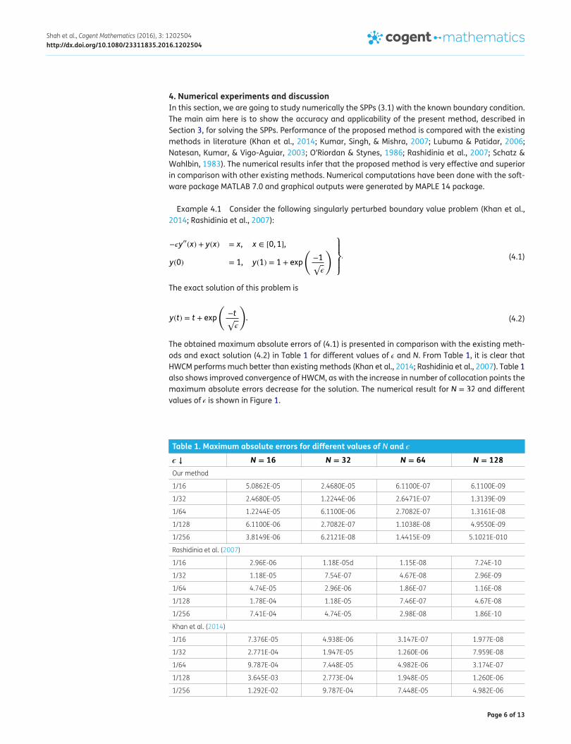
4. Numerical experiments and discussionIn this section, we are going to study numerically the SPPs (3.1) with the known boundary condition. The main aim here is to show the accuracy and applicability of the present method, described in Section 3, for solving the SPPs. Performance of the proposed method is compared with the existing methods in literature (Khan et al., 2014; Kumar, Singh, & Mishra, 2007; Lubuma & Patidar, 2006; Natesan, Kumar, & Vigo-Aguiar, 2003; O’Riordan & Stynes, 1986; Rashidinia et al., 2007; Schatz & Wahlbin, 1983). The numerical results infer that the proposed method is very effective and superior in comparison with other existing methods. Numerical computations have been done with the soft-ware package MATLAB 7.0 and graphical outputs were generated by MAPLE 14 package.

Example 4.1 Consider the following singularly perturbed boundary value problem (Khan et al., 2014; Rashidinia et al., 2007):

The exact solution of this problem is

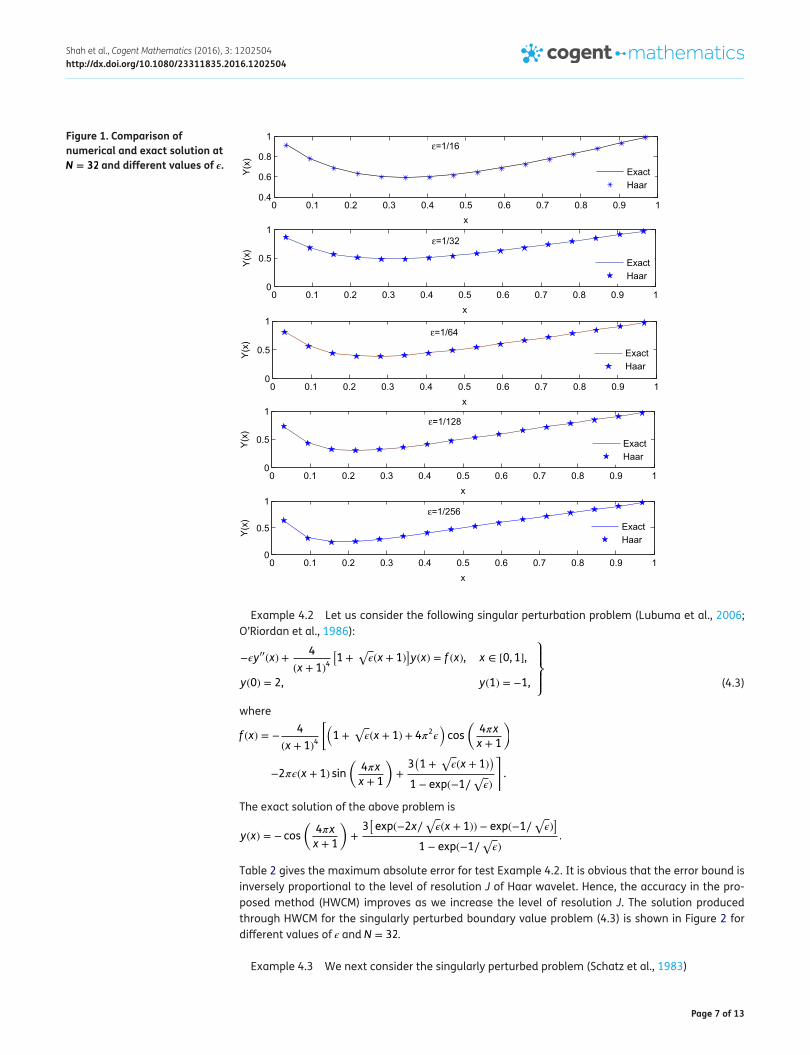
The obtained maximum absolute errors of (4.1) is presented in comparison with the existing meth-ods and exact solution (4.2) in Table 1 for different values of � and N. From Table 1, it is clear that HWCM performs much better than existing methods (Khan et al., 2014; Rashidinia et al., 2007). Table 1 also shows improved convergence of HWCM, as with the increase in number of collocation points the maximum absolute errors decrease for the solution. The numerical result for N = 32 and different values of � is shown in Figure 1.

(4.1)−�y��(x) + y(x) = x, x ∈ [0, 1],

y(0) = 1, y(1) = 1 + exp

�−1√�

� ⎫⎪⎬⎪⎭.

(4.2)y(t) = t + exp

�−t√�

�.

Table 1. Maximum absolute errors for different values of N and �� ↓ N = 16 N = 32 N = 64 N = 128

Our method

1/16 5.0862E-05 2.4680E-05 6.1100E-07 6.1100E-09

1/32 2.4680E-05 1.2244E-06 2.6471E-07 1.3139E-09

1/64 1.2244E-05 6.1100E-06 2.7082E-07 1.3161E-08

1/128 6.1100E-06 2.7082E-07 1.1038E-08 4.9550E-09

1/256 3.8149E-06 6.2121E-08 1.4415E-09 5.1021E-010

Rashidinia et al. (2007)

1/16 2.96E-06 1.18E-05d 1.15E-08 7.24E-10

1/32 1.18E-05 7.54E-07 4.67E-08 2.96E-09

1/64 4.74E-05 2.96E-06 1.86E-07 1.16E-08

1/128 1.78E-04 1.18E-05 7.46E-07 4.67E-08

1/256 7.41E-04 4.74E-05 2.98E-08 1.86E-10

Khan et al. (2014)

1/16 7.376E-05 4.938E-06 3.147E-07 1.977E-08

1/32 2.771E-04 1.947E-05 1.260E-06 7.959E-08

1/64 9.787E-04 7.448E-05 4.982E-06 3.174E-07

1/128 3.645E-03 2.773E-04 1.948E-05 1.260E-06

1/256 1.292E-02 9.787E-04 7.448E-05 4.982E-06

Page 7 of 13


Example 4.2 Let us consider the following singular perturbation problem (Lubuma et al., 2006; O’Riordan et al., 1986):

where

The exact solution of the above problem is

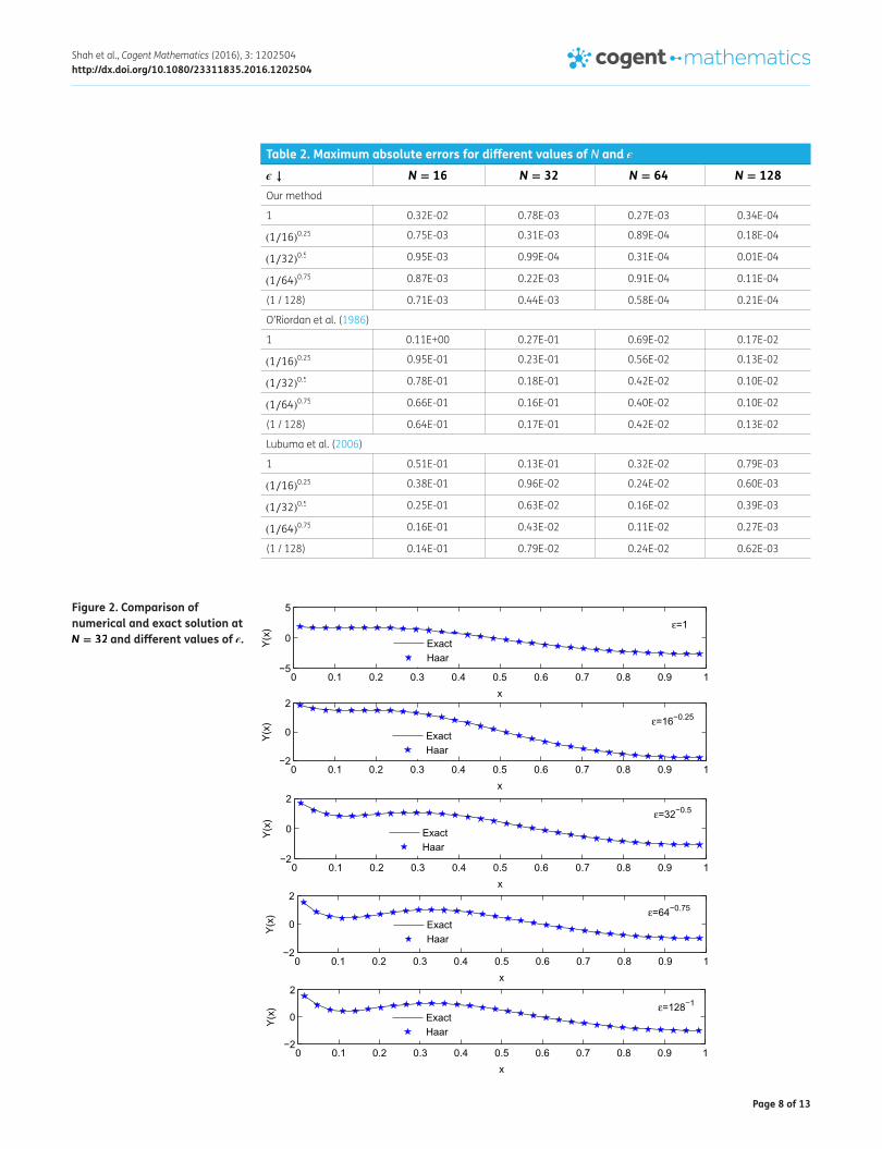
Table 2 gives the maximum absolute error for test Example 4.2. It is obvious that the error bound is inversely proportional to the level of resolution J of Haar wavelet. Hence, the accuracy in the pro-posed method (HWCM) improves as we increase the level of resolution J. The solution produced through HWCM for the singularly perturbed boundary value problem (4.3) is shown in Figure 2 for different values of � and N = 32.

Example 4.3 We next consider the singularly perturbed problem (Schatz et al., 1983)

(4.3)

−�y��(x) +4

(x + 1)4�1 +

√�(x + 1)

�y(x) = f (x), x ∈ [0, 1],

y(0) = 2, y(1) = −1,

⎫⎪⎬⎪⎭

f (x) = −4

(x + 1)4

��1 +

√�(x + 1) + 4�2�

�cos

�4�x

x + 1

�

−2��(x + 1) sin

�4�x

x + 1

�+3�1 +

√�(x + 1)

�

1 − exp(−1∕√�)

�.

y(x) = − cos

�4�x

x + 1

�+3�exp(−2x∕

√�(x + 1)) − exp(−1∕

√�)�

1 − exp(−1∕√�)

.

Figure 1. Comparison of numerical and exact solution at N = 32 and different values of �.

0 0.1 0.2 0.3 0.4 0.5 0.6 0.7 0.8 0.9 10.4

0.6

0.8

1

x

Y(x)

0 0.1 0.2 0.3 0.4 0.5 0.6 0.7 0.8 0.9 10

0.5

1

x

Y(x)

0 0.1 0.2 0.3 0.4 0.5 0.6 0.7 0.8 0.9 10

0.5

1

x

Y(x)

0 0.1 0.2 0.3 0.4 0.5 0.6 0.7 0.8 0.9 10

0.5

1

x

Y(x)

0 0.1 0.2 0.3 0.4 0.5 0.6 0.7 0.8 0.9 10

0.5

1

x

Y(x)

ExactHaar

ExactHaar

ExactHaar

ExactHaar

ExactHaar

=1/16

=1/32

=1/64

=1/128

=1/256

Page 8 of 13



Our method

1 0.32E-02 0.78E-03 0.27E-03 0.34E-04

(1∕16)0.25 0.75E-03 0.31E-03 0.89E-04 0.18E-04

(1∕32)0.5 0.95E-03 0.99E-04 0.31E-04 0.01E-04

(1∕64)0.75 0.87E-03 0.22E-03 0.91E-04 0.11E-04

(1 / 128) 0.71E-03 0.44E-03 0.58E-04 0.21E-04

O’Riordan et al. (1986)

1 0.11E+00 0.27E-01 0.69E-02 0.17E-02

(1∕16)0.25 0.95E-01 0.23E-01 0.56E-02 0.13E-02

(1∕32)0.5 0.78E-01 0.18E-01 0.42E-02 0.10E-02

(1∕64)0.75 0.66E-01 0.16E-01 0.40E-02 0.10E-02

(1 / 128) 0.64E-01 0.17E-01 0.42E-02 0.13E-02

Lubuma et al. (2006)

1 0.51E-01 0.13E-01 0.32E-02 0.79E-03

(1∕16)0.25 0.38E-01 0.96E-02 0.24E-02 0.60E-03

(1∕32)0.5 0.25E-01 0.63E-02 0.16E-02 0.39E-03

(1∕64)0.75 0.16E-01 0.43E-02 0.11E-02 0.27E-03

(1 / 128) 0.14E-01 0.79E-02 0.24E-02 0.62E-03

Figure 2. Comparison of numerical and exact solution at N = 32 and different values of �.

0 0.1 0.2 0.3 0.4 0.5 0.6 0.7 0.8 0.9 1−5

0

5

x

Y(x)

0 0.1 0.2 0.3 0.4 0.5 0.6 0.7 0.8 0.9 1−2

0

2

x

Y(x)

0 0.1 0.2 0.3 0.4 0.5 0.6 0.7 0.8 0.9 1−2

0

2

x

Y(x)

0 0.1 0.2 0.3 0.4 0.5 0.6 0.7 0.8 0.9 1−2

0

2

x

Y(x)

0 0.1 0.2 0.3 0.4 0.5 0.6 0.7 0.8 0.9 1−2

0

2

x

Y(x)

ExactHaar

ExactHaar

ExactHaar

ExactHaar

ExactHaar

=1

=16−0.25

=32−0.5

=64−0.75

=128−1

Page 9 of 13


whose exact solution is given by

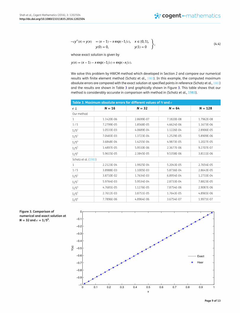
We solve this problem by HWCM method which developed in Section 2 and compare our numerical results with finite element method (Schatz et al., 1983). In this example, the computed maximum absolute errors are compared with the exact solution at specified points in reference (Schatz et al., 1983) and the results are shown in Table 3 and graphically shown in Figure 3. This table shows that our method is considerably accurate in comparison with method in (Schatz et al., 1983).

(4.4)−�y��(x) + y(x) = (x − 1) − x exp(−1∕�), x ∈ [0, 1],

y(0) = 0, y(1) = 0

},

y(x) = (x − 1) − x exp(−1∕�) + exp(−x∕�).


Our method

1 1.1420E-06 2.8699E-07 7.1820E-08 1.7962E-08

1 / 5 7.2799E-05 1.8568E-05 4.6624E-06 1.1673E-06

1∕52 1.0533E-03 4.0689E-04 1.1226E-04 2.8906E-05

1∕53 7.0483E-03 1.3723E-04 1.2529E-05 5.8909E-06

1∕54 3.6848E-04 1.4255E-04 4.9873E-05 1.2027E-05

1∕55 1.4897E-05 5.9510E-06 2.3677E-06 9.2707E-07

1∕56 5.9615E-05 2.3845E-05 9.5358E-06 3.8111E-06

Schatz et al. (1983)

1 2.2123E-04 1.9925E-04 5.2043E-05 2.7654E-05

1 / 5 3.8988E-03 1.1005E-03 5.8736E-04 2.8643E-05

1∕52 3.8710E-02 1.7634E-03 6.8954E-04 1.2733E-04

1∕53 5.9764E-03 5.9534E-04 2.8733E-04 7.8823E-05

1∕54 4.7681E-05 1.1276E-05 7.8754E-06 2.9087E-06

1∕55 2.7612E-03 3.8751E-05 1.7643E-05 4.8965E-06

1∕56 7.7896E-06 4.8964E-06 3.6754E-07 1.9971E-07

Figure 3. Comparison of numerical and exact solution at N = 32 and � = 1∕5

6.

0 0.1 0.2 0.3 0.4 0.5 0.6 0.7 0.8 0.9 1−1

−0.9

−0.8

−0.7

−0.6

−0.5

−0.4

−0.3

−0.2

−0.1

0

x

Y(x

)

Exact

Haar

Page 10 of 13


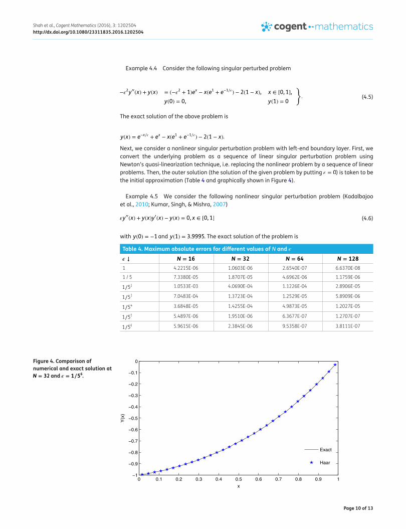
Example 4.4 Consider the following singular perturbed problem

The exact solution of the above problem is

Next, we consider a nonlinear singular perturbation problem with left-end boundary layer. First, we convert the underlying problem as a sequence of linear singular perturbation problem using Newton’s quasi-linearization technique, i.e. replacing the nonlinear problem by a sequence of linear problems. Then, the outer solution (the solution of the given problem by putting � = 0) is taken to be the initial approximation (Table 4 and graphically shown in Figure 4).

Example 4.5 We consider the following nonlinear singular perturbation problem (Kadalbajoo et al., 2010; Kumar, Singh, & Mishra, 2007)

with y(0) = −1 and y(1) = 3.9995. The exact solution of the problem is

(4.5)−�

2y��(x) + y(x) = (−�2+ 1)ex − x(e1 + e−1∕�) − 2(1 − x), x ∈ [0, 1],

y(0) = 0, y(1) = 0

}.

y(x) = e−x∕� + ex − x(e1 + e−1∕�) − 2(1 − x).

(4.6)�y��(x) + y(x)y�(x) − y(x) = 0, x ∈ [0, 1]


1 4.2215E-06 1.0603E-06 2.6540E-07 6.6370E-08

1 / 5 7.3380E-05 1.8707E-05 4.6962E-06 1.1759E-06

1∕52 1.0533E-03 4.0690E-04 1.1226E-04 2.8906E-05

1∕53 7.0483E-04 1.3723E-04 1.2529E-05 5.8909E-06

1∕54 3.6848E-05 1.4255E-04 4.9873E-05 1.2027E-05

1∕55 5.4897E-06 1.9510E-06 6.3677E-07 1.2707E-07

1∕56 5.9615E-06 2.3845E-06 9.5358E-07 3.8111E-07

Figure 4. Comparison of numerical and exact solution at N = 32 and � = 1∕5

6.

0 0.1 0.2 0.3 0.4 0.5 0.6 0.7 0.8 0.9 1−1

−0.9

−0.8

−0.7

−0.6

−0.5

−0.4

−0.3

−0.2

−0.1

0

x

Y(x

)

Exact

Haar

Page 11 of 13


where c1 = 2.9995 and c2 = (1∕c1) loge[(c1 − 1)∕(c1 + 1)].

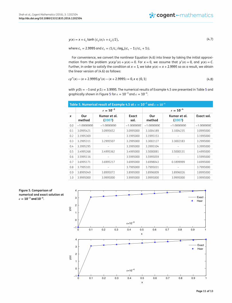
For convenience, we convert the nonlinear Equation (4.6) into linear by taking the initial approxi-mation from the problem y(x)y�(x) + y(x) = 0. For x = 0, we assume that y�(x) = 0, and y(x) = C. Further, in order to satisfy the condition at x = 1, we take y(x) = x + 2.9995 so as a result, we obtain the linear version of (4.6) as follows:

with y(0) = −1 and y(1) = 3.9995. The numerical results of Example 4.5 are presented in Table 5 and graphically shown in Figure 5 for � = 10−3 and � = 10−4.

(4.7)y(x) = x + c1 tanh(c1(x∕� + c2)∕2

),

(4.8)�y��(x) − (x + 2.9995)y�(x) − (x + 2.9995) = 0, x ∈ [0, 1]

Table 5. Numerical result of Example 4.5 at � = 10−3 and � = 10

−4

� = 10−3

� = 10−4

x Our method

Kumar et al. (2007)

Exact sol.

Our method

Kumar et al. (2007)

Exact sol.

0.0 −1.0000000 −1.0000000 −1.0000000 −1.0000000 −1.0000000 −1.0000000

0.1 3.0995421 3.0995652 3.0995000 3.1004189 3.1004235 3.0995000

0.2 3.1995369 – 3.1995000 3.1995153 – 3.1995000

0.3 3.2995311 3.2995507 3.2995000 3.3002127 3.3002183 3.2995000

0.4 3.3995295 – 3.3995000 3.3995104 – 3.3995000

0.5 3.4995268 3.4995362 3.4995000 3.5000081 3.5000131 3.4995000

0.6 3.5995116 – 3.5995000 3.5995059 – 3.5995000

0.7 3.6995171 3.6995217 3.6995000 3.6998043 0.1899999 3.6995000

0.8 3.7995101 – 3.7995000 3.7995031 – 3.7995000

0.9 3.8995049 3.8995072 3.8995000 3.8996009 3.8996026 3.8995000

1.0 3.9995000 3.9995000 3.9995000 3.9995000 3.9995000 3.9995000

Figure 5. Comparison ofnumerical and exact solution at � = 10

−3and10

−4.

0 0.1 0.2 0.3 0.4 0.5 0.6 0.7 0.8 0.9 1−1

0

1

2

3

4

x

y(x)

ExactHaar

0 0.1 0.2 0.3 0.4 0.5 0.6 0.7 0.8 0.9 1−1

0

1

2

3

4

x

y(x)

ExactHaar

ε=10−4

ε=10−3

Page 12 of 13


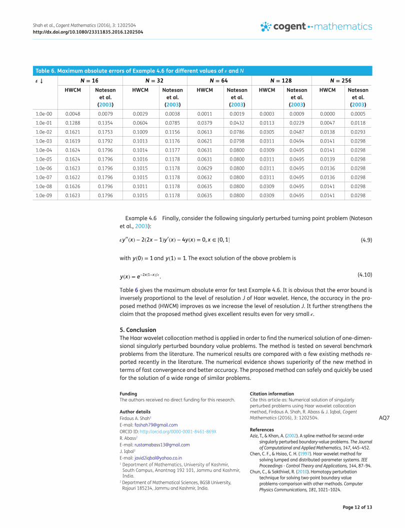
Example 4.6 Finally, consider the following singularly perturbed turning point problem (Natesan et al., 2003):

with y(0) = 1 and y(1) = 1. The exact solution of the above problem is

Table 6 gives the maximum absolute error for test Example 4.6. It is obvious that the error bound is inversely proportional to the level of resolution J of Haar wavelet. Hence, the accuracy in the pro-posed method (HWCM) improves as we increase the level of resolution J. It further strengthens the claim that the proposed method gives excellent results even for very small �.

5. ConclusionThe Haar wavelet collocation method is applied in order to find the numerical solution of one-dimen-sional singularly perturbed boundary value problems. The method is tested on several benchmark problems from the literature. The numerical results are compared with a few existing methods re-ported recently in the literature. The numerical evidence shows superiority of the new method in terms of fast convergence and better accuracy. The proposed method can safely and quickly be used for the solution of a wide range of similar problems.

(4.9)�y��(x) − 2(2x − 1)y�(x) − 4y(x) = 0, x ∈ [0, 1]

(4.10)y(x) = e−2x(1−x)∕�.

FundingThe authors received no direct funding for this research.

Author detailsFirdous A. Shah1

E-mail: [email protected] ID: http://orcid.org/0000-0001-8461-869XR. Abass2

E-mail: [email protected]. Iqbal2

E-mail: [email protected] Department of Mathematics, University of Kashmir,

South Campus, Anantnag 192 101, Jammu and Kashmir, India.

2 Department of Mathematical Sciences, BGSB University, Rajouri 185234, Jammu and Kashmir, India.

Citation informationCite this article as: Numerical solution of singularly perturbed problems using Haar wavelet collocation method, Firdous A. Shah, R. Abass & J. Iqbal, Cogent Mathematics (2016), 3: 1202504.

ReferencesAziz, T., & Khan, A. (2002). A spline method for second-order

singularly perturbed boundary-value problems. The Journal of Computational and Applied Mathematics, 147, 445–452.

Chen, C. F., & Hsiao, C. H. (1997). Haar wavelet method for solving lumped and distributed-parameter systems. IEE Proceedings - Control Theory and Applications, 144, 87–94.

Chun, C., & Sakthivel, R. (2010). Homotopy perturbation technique for solving two-point boundary value problems-comparison with other methods. Computer Physics Communications, 181, 1021–1024.

Table 6. Maximum absolute errors of Example 4.6 for different values of � and N� ↓ N = 16 N = 32 N = 64 N = 128 N = 256

HWCM Natesan et al.

(2003)

HWCM Natesan et al.

(2003)

HWCM Natesan et al.

(2003)

HWCM Natesan et al.

(2003)

HWCM Natesan et al.

(2003)1.0e-00 0.0048 0.0079 0.0029 0.0038 0.0011 0.0019 0.0003 0.0009 0.0000 0.0005

1.0e-01 0.1288 0.1354 0.0604 0.0785 0.0379 0.0432 0.0113 0.0229 0.0047 0.0118

1.0e-02 0.1621 0.1753 0.1009 0.1156 0.0613 0.0786 0.0305 0.0487 0.0138 0.0293

1.0e-03 0.1619 0.1792 0.1013 0.1176 0.0621 0.0798 0.0311 0.0494 0.0141 0.0298

1.0e-04 0.1624 0.1796 0.1014 0.1177 0.0631 0.0800 0.0309 0.0495 0.0141 0.0298

1.0e-05 0.1624 0.1796 0.1016 0.1178 0.0631 0.0800 0.0311 0.0495 0.0139 0.0298

1.0e-06 0.1623 0.1796 0.1015 0.1178 0.0629 0.0800 0.0311 0.0495 0.0136 0.0298

1.0e-07 0.1622 0.1796 0.1015 0.1178 0.0632 0.0800 0.0311 0.0495 0.0136 0.0298

1.0e-08 0.1626 0.1796 0.1011 0.1178 0.0635 0.0800 0.0309 0.0495 0.0141 0.0298

1.0e-09 0.1623 0.1796 0.1015 0.1178 0.0635 0.0800 0.0309 0.0495 0.0141 0.0298

AQ7


http://orcid.org/0000-0001-8461-869X



Page 13 of 13


© 2016 The Author(s). This open access article is distributed under a Creative Commons Attribution (CC-BY) 4.0 license.You are free to: Share — copy and redistribute the material in any medium or format Adapt — remix, transform, and build upon the material for any purpose, even commercially.The licensor cannot revoke these freedoms as long as you follow the license terms.

Under the following terms:Attribution — You must give appropriate credit, provide a link to the license, and indicate if changes were made. You may do so in any reasonable manner, but not in any way that suggests the licensor endorses you or your use. No additional restrictions You may not apply legal terms or technological measures that legally restrict others from doing anything the license permits.

Daubechies, I. (1992). Ten Lectures on Wavelets. Philadelphia: SIAM.

Debnath, L., & Shah, F. A. (2015). Wavelet transforms and their applications. New York, NY: Birkhäuser.

Geng, F. Z., & Cui, M. G. (2011). A novel method for solving a class of singularly perturbed boundary value problems based on reproducing kernel method. Applied Mathematics and Computation, 218, 4211–4215.

Kadalbajoo, M. K., & Arora, P. (2010). B-splines with artificial viscosity for solving singularly perturbed boundary value problems. Mathematical and Computer Modelling, 52, 654–666.

Kadalbajoo, M. K., & Gupta, V. (2009). Numerical solution of singularly perturbed convection-diffusion problem using parameter uniform B-spline collocation method. The Journal of Mathematical Analysis and Applications, 355, 439–452.

Kadalbajoo, M. K., Gupta, V., & Awasthi, A. (2008). A uniformly convergent B-spline collocation method on a nonuniform mesh for singularly perturbed one-dimensional time-dependent linear convection-diffusion problem. The Journal of Computational and Applied Mathematics, 220, 271–289.

Khan, A., Khan, I., & Aziz, T. (2006). Sextic spline solution of singularly perturbed boundary-value problems. Applied Mathematics and Computation, 181, 432–439.

Khan, A., & Khandelwala, P. (2014). Non-polynomial sextic spline solution of singularly perturbed boundary-value problems. International Journal of Computer Mathematics, 91, 1122–1135.

Kumar, V., & Mehra, M. (2007). Cubic spline adaptive wavelet scheme to solve singularly perturbed reaction diffusion problems. International Journal of Wavelets, Multiresolution and Information Processing, 5, 317–331.

Kumar, M., Singh, P., & Mishra, H. K. (2007). An initial-value technique for singularly perturbed boundary value problems via cubic spline. International Journal for Computational Methods in Engineering Science and Mechanics, 8, 419–427.

Lenferink, W. (2002). A second order scheme for a time-dependent, singularly perturbed convection-diffusion equation. The Journal of Computational and Applied Mathematics, 143, 49–68.

Lepik, U. (2008). Solving integral and differential equations by the aid of nonuniform Haar wavelets. Applied Mathematics and Computation, 198, 326–332.

Lepik, U., & Hein, H. (2014). Haar wavelets with applications. New York, NY: Springer.

Lubuma, J. S., & Patidar, K. C. (2006). Uniformly convergent non-standard finite difference methods for self-adjoint singular perturbation problems. The Journal of Computational and Applied Mathematics, 191, 228–238.

Miller, J. H., O’Riordan, E., & Shishkin, G. I. (1996). Fitted numerical methods for singular perturbation problems. Singapore: World Scientific.

Mohsen, A., & EL-Gamel, M. (2008). On the Galerkin and collocation methods for two-point boundary value problem using Sinc bases. International Journal of Computer Mathematics, 56, 930–941.

Natesan, S., Kumar, J. J., & Vigo-Aguiar, J. (2003). Parameter uniform numerical method for singularly perturbed turning point problems exhibiting boundary layers. The Journal of Computational and Applied Mathematics, 158, 121–134.

O’Riordan, E., & Stynes, M. (1986). A uniformly accurate finite-element method for a singularly perturbed one-dimensional reaction-diffusion problem. Mathematics of Computation, 47, 555–570.

Pandit, S., & Kumar, M. (2014). Haar wavelet approach for numerical solution of two parameters singularly perturbed boundary value problems. Applied Mathematics & Information Sciences, 8, 2965–2974.

Phongthanapanich, S., & Dechaumphai, P. (2009). Combined finite volume element method for singularly perturbed reaction-diffusion problems. Applied Mathematics and Computation, 209, 177–185.

Rashidinia, J., Ghasemi, M., & Mahmoodi, Z. (2007). Spline approach to the solution of a singularly-perturbed boundary-value problems. Applied Mathematics and Computation, 189, 72–78.

Roos, H. G., Stynes, M., & Tobiska, L. (1996). Numerical Methods for singularly perturbed differential equations. New York, NY: Springer.

Schatz, A. H., & Wahlbin, L. B. (1983). On the finite element method for singularly perturbed reaction-diffusion problems in two and one dimensions. Mathematics of Computation, 40, 47–89.

Surla, K., & Stojanovic, M. (1988). Solving singularly-perturbed boundary-value problems by splines in tension. The Journal of Computational and Applied Mathematics, 24, 355–363.

Wazwaz, A. M. (2002). A new method for solving singular initial value problems in the second-order ordinary differential equations. Applied Mathematics and Computation, 128, 45–57.

Documents

Numerical solution of singularly perturbed problems … · Shah et al., Cogent Mathematics (2016), 3: 1202504 APPLIED & INTERDISCIPLINARY MATHEMATICS | RESEARCH ARTICLE Numerical