“Computing is not about computers anymore. It is aboutstaff.cs.psu.ac.th/sathit/ComOr/Ch1Intro.pdf · •Peta- (P) = 1 quadrillion ... • Hertz = clock cycles per second (frequency)

1

2

“Computing is not about computers anymore. It is about

living…. We have seen computers move out of giant air-

conditioned rooms into closets, then onto desktops, and

now into our laps and pockets. But this is not the end….

Like a force of nature, the digital age cannot be denied or

stopped…. The information superhighway may be mostly

hype today, but it is an understatement about tomorrow. It

will exist beyond people’s wildest predictions…. We are

not waiting on any invention. It is here. It is now. It is

almost genetic in its nature, in that each generation will

become more digital than the preceding one.”

—Nicholas Negroponte, professor of media technology at

MIT

3

Chapter 1 Objectives

Computer organization and architecture.

Units of measure common to computer systems.

Computer as a layered system.

Components von Neumann architecture and the

function of basic computer components.

Cloud computing

Parallel computer

4

Why study computer organization and

architecture?

– Design better programs, including system software

such as compilers, operating systems, and device

drivers.

– Optimize program behavior.

– Evaluate (benchmark) computer system performance.

– Understand time, space, and price tradeoffs.

1.1 Overview

5

1.1 Overview

• Computer organization

– physical aspects of computer systems.

– E.g., circuit design, control signals, memory types.

– How does a computer work?

• Computer architecture

– Logical aspects of system as seen by the programmer.

– E.g., instruction sets, instruction formats, data types,

addressing modes.

– How do I design a computer?

6

1.1 Overview

Com Org. vs Com Arch.

• Distinction between computer organization and computer

architecture is not clear-cut.

• Computer science and computer engineering hold

differing opinions,

– they can stand alone;

– are interrelated and interdependent.

• Comprehension of com org and arch ultimately

leads to a deeper understanding of computers and

computation

– the heart and soul of computer science.

7

1.2 Computer Components

• Principle of Equivalence of Hardware and

Software:

– Anything that can be done with

software can also be done with

hardware, and anything that can be

done with hardware can also be

done with software.*

* Assuming speed is not a concern.

8

• At the most basic level, a computer is a

device consisting of three pieces:

– A processor to interpret and execute

programs

– A memory to store both data and programs

– A mechanism for transferring data to and

from the outside world.

1.2 Computer Components

9

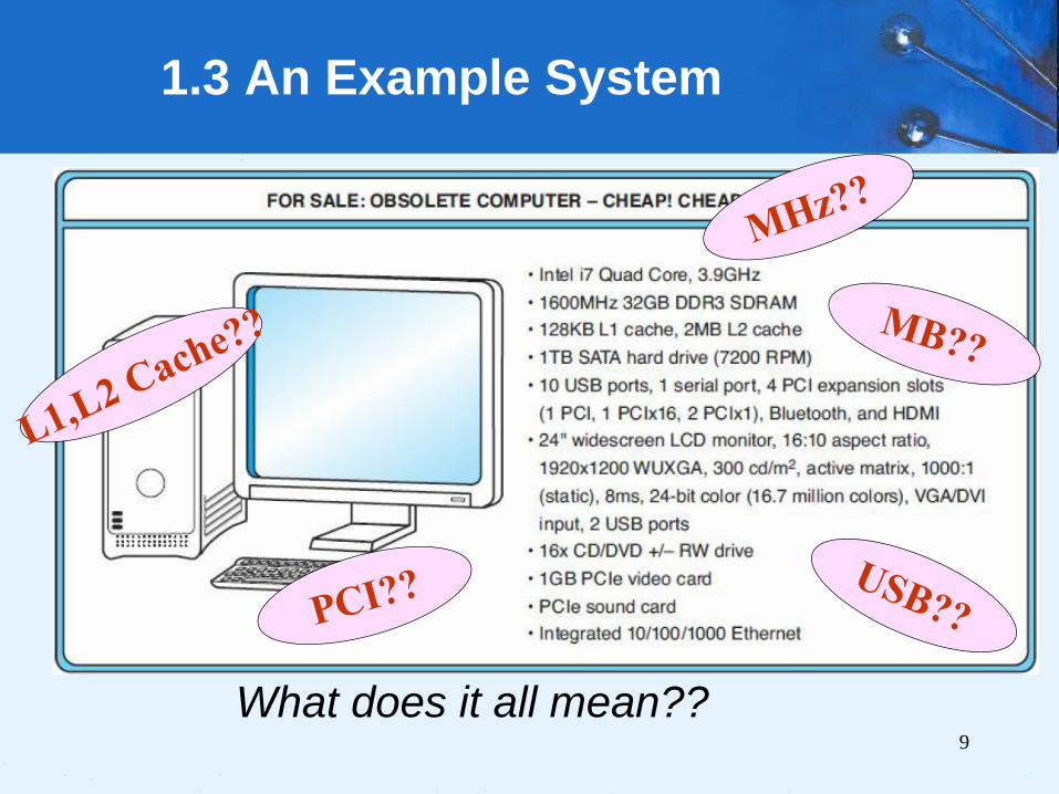
1.3 An Example System

What does it all mean??

10

Measures of capacity and speed:

• Kilo- (K) = 1 thousand = 103 and 210

• Mega- (M) = 1 million = 106 and 220

• Giga- (G) = 1 billion = 109 and 230

• Tera- (T) = 1 trillion = 1012 and 240

• Peta- (P) = 1 quadrillion = 1015 and 250


11

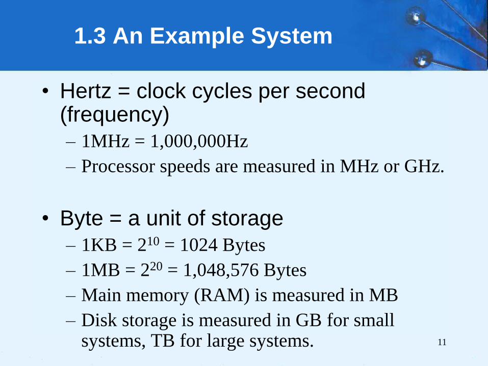
• Hertz = clock cycles per second (frequency)

– 1MHz = 1,000,000Hz

– Processor speeds are measured in MHz or GHz.

• Byte = a unit of storage

– 1KB = 210 = 1024 Bytes

– 1MB = 220 = 1,048,576 Bytes

– Main memory (RAM) is measured in MB

– Disk storage is measured in GB for small systems, TB for large systems.


12


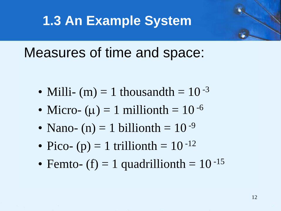
Measures of time and space:

• Milli- (m) = 1 thousandth = 10 -3

• Micro- () = 1 millionth = 10 -6

• Nano- (n) = 1 billionth = 10 -9

• Pico- (p) = 1 trillionth = 10 -12

• Femto- (f) = 1 quadrillionth = 10 -15

13

• Millisecond = 1 thousandth of a second

– Hard disk drive access times are often 10 to 20

milliseconds.

• Nanosecond = 1 billionth of a second

– Main memory access times are often 50 to 70

nanoseconds.

• Micron (micrometer) = 1 millionth of a

meter

– Circuits on computer chips are measured in

microns.


14

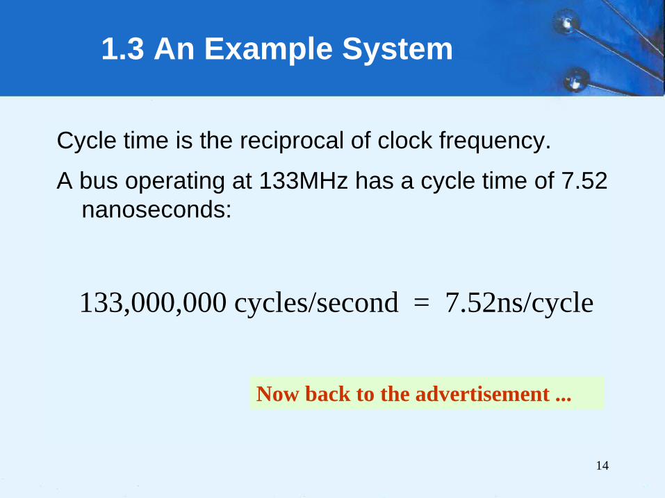
Cycle time is the reciprocal of clock frequency.

A bus operating at 133MHz has a cycle time of 7.52

nanoseconds:


Now back to the advertisement ...

133,000,000 cycles/second = 7.52ns/cycle

15

16

17

18

19


A system bus moves data within the

computer. The faster the bus the better.

This one runs at 1600MHz.

memory capacity of 32 GB

DDR3 SDRAM, or double data

rate type three synchronous

dynamic RAM

The microprocessor is the

“brain” of the system. It

executes program instructions.

This one is a Pentium (Intel,

i7) Quad core =>multicore

processors, running at 3.9

GHz.

20


• Large main memory capacity means

you can run larger programs with

greater speed than computers having

small memories.

• RAM = random access memory. Time

to access contents is independent of its

location.

• Cache is a type of temporary memory

that can be accessed faster than RAM.

21


… and two levels of cache memory, the level 1 (L1: that

is built into the microprocessor chip and helps speed up

access to frequently used data.) L1 is smaller and

(probably) faster than the L2 cache that is built-in

memory chips situated between the microprocessor and

main memory.

“128KB L1 cache, 2MB L2

cache” also describes a type of

memory.

To provide even faster access to

data, many systems contain a

special memory called cache.

22


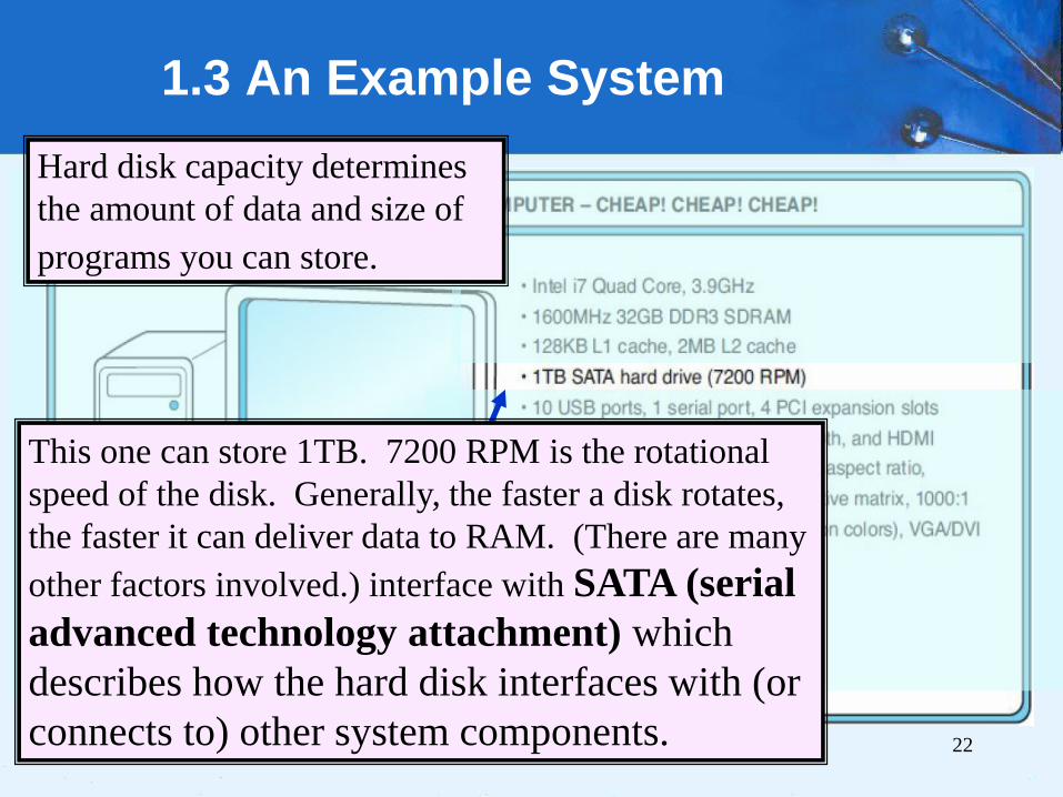
This one can store 1TB. 7200 RPM is the rotational

speed of the disk. Generally, the faster a disk rotates,

the faster it can deliver data to RAM. (There are many

other factors involved.) interface with SATA (serial

advanced technology attachment) which

describes how the hard disk interfaces with (or

connects to) other system components.

Hard disk capacity determines

the amount of data and size of

programs you can store.

23


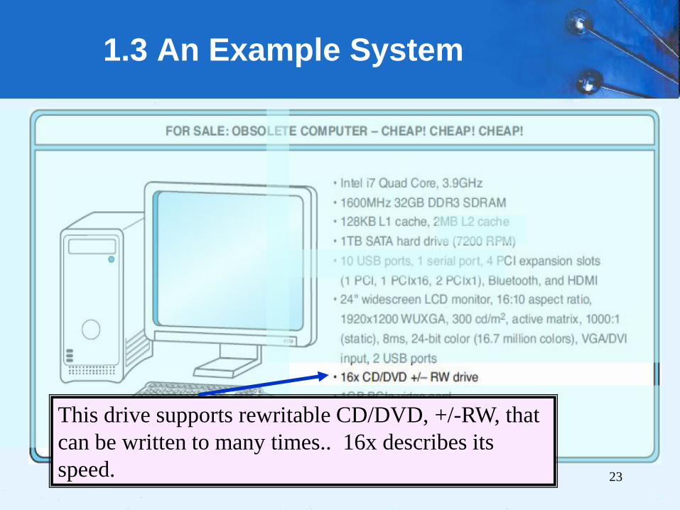
This drive supports rewritable CD/DVD, +/-RW, that

can be written to many times.. 16x describes its

speed.

24


Expansion slots

System buses can be augmented by dedicated I/O buses. PCI,

peripheral component interface, is one such bus.

HDMI port (High-Definition Multimedia Interface, used to

transmit audio and video).

ports

allow movement of data to and

from devices external to the

computer.

“10 USB ports, 1 serial port.” Serial

ports transfer data by sending a series of

electrical pulses across one or two data

lines.

25


• Serial ports send data as a series of

pulses along one or two data lines.

• Parallel ports send data as a single

pulse along at least eight data lines.

• USB, Universal Serial Bus, is an

intelligent serial interface that is self-

configuring. (It supports “plug and

play.”)

26


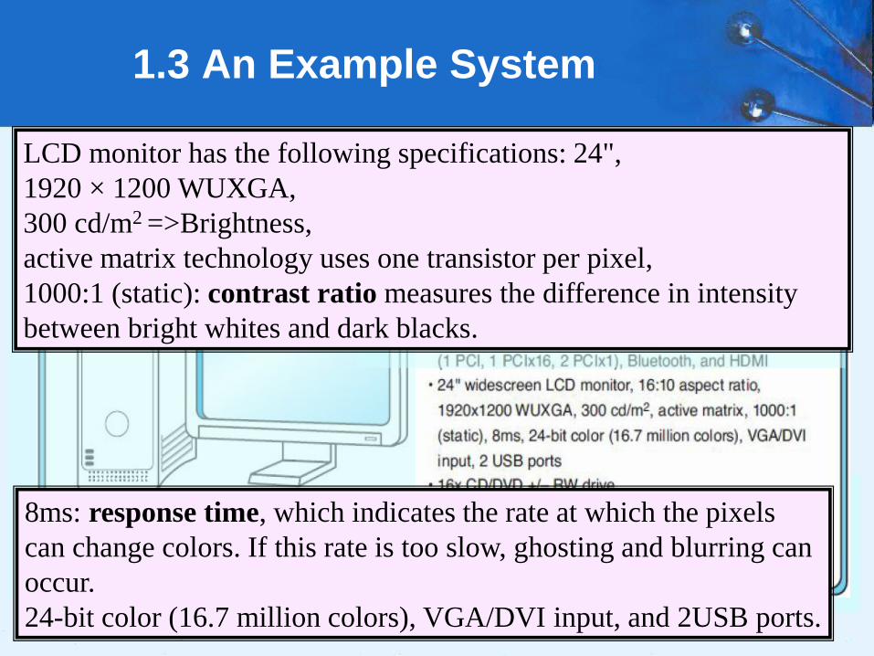
8ms: response time, which indicates the rate at which the pixels

can change colors. If this rate is too slow, ghosting and blurring can

occur.

24-bit color (16.7 million colors), VGA/DVI input, and 2USB ports.

LCD monitor has the following specifications: 24",

1920 × 1200 WUXGA,

300 cd/m2 =>Brightness,

active matrix technology uses one transistor per pixel,

1000:1 (static): contrast ratio measures the difference in intensity

between bright whites and dark blacks.


27

28


PCIe video card with 1GB of memory. The memory is used by a

special graphics processing unit on the card. This processor is

responsible for performing the necessary calculations to render the

graphics so the main processor of the computer is not required to

do so.

PCIe sound card; a sound card

contains components needed

by the system’s stereo speakers

and microphone.

29


network interface card (NIC), which connects to the

motherboard via a PCI slot. NICs typically support 10/100

Ethernet (both Ethernet at a speed of 10Mbps and fast

Ethernet at a speed of 100Mbps) or 10/100/1000 (which adds

Ethernet at 1,000Mbps).


Basic performance characteristics of

computer systems, including:

1. Processor speed,

2. Memory speed,

3. Memory capacity, and

4. Interconnection data rates

30

31

• The evolution of computing

machinery has taken place over

several centuries.

• The evolution of computers is

usually classified into different

generations according to the

technology of the era.

1.5 Historical Development

32

Generation Zero: Mechanical Calculating Machines

(1642 - 1945)

– Calculating Clock - Wilhelm Schickard (1592 - 1635).


Rechenuhr (calculating clock).

The machine was designed to

assist in all the four basic

functions of arithmetic (addition,

subtraction, multiplication and

division).

Cr:

https://en.wikipedia.org/wiki/Wilhelm_Sc

hickard

33


(1642 - 1945)

– Pascaline - Blaise Pascal (1623 - 1662).


mechanical calculator

capable of addition and

subtraction, called Pascal's

calculator or the Pascaline.

Cr:

https://en.wikipedia.org/wik

i/Blaise_Pascal

34


(1642 - 1945)

– Difference Engine - Charles Babbage (1791 - 1871),

also designed but never built the Analytical Engine.


Babbage's design. The design

has the same precision on all

columns, but when calculating

polynomials, the precision on

the higher-order columns could

be lower.

Cr:

https://en.wikipedia.org/wiki/Dif

ference_engine

35


(1642 - 1945)

– Punched card tabulating machines - Herman Hollerith

(1860 - 1929).

Hollerith cards were commonly used for

computer input well into the 1970s.


The tabulating machine was

an electromechanical machine designed

to assist in summarizing information

stored on punched cards.

Cr:

https://en.wikipedia.org/wiki/Tabulating

_machine

36

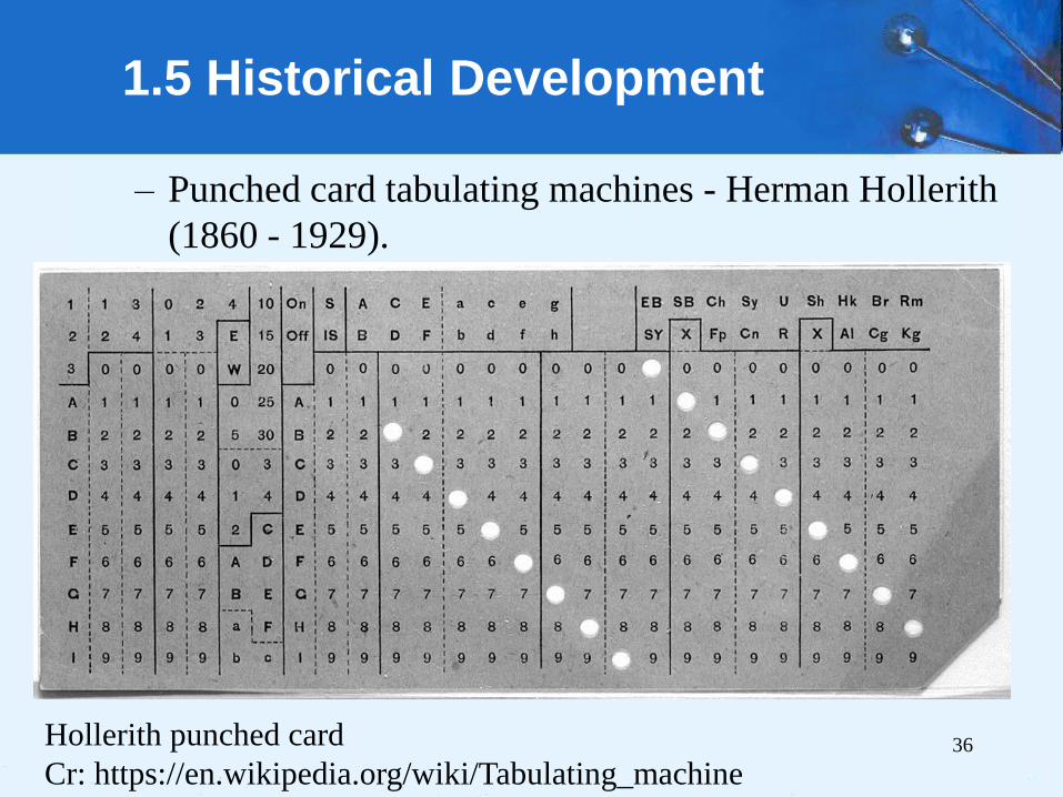
– Punched card tabulating machines - Herman Hollerith

(1860 - 1929).


Hollerith punched card

Cr: https://en.wikipedia.org/wiki/Tabulating_machine

37

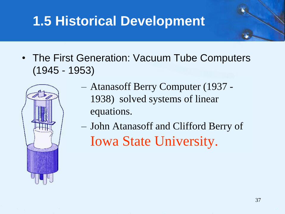
• The First Generation: Vacuum Tube Computers

(1945 - 1953)

– Atanasoff Berry Computer (1937 -

1938) solved systems of linear

equations.

– John Atanasoff and Clifford Berry of

Iowa State University.


38

• The First Generation:

Vacuum Tube

Computers (1945 -

1953)

Electronic Numerical

Integrator and Computer

(ENIAC) by John

Mauchly and J. Presper

Eckertat the University

of Pennsylvania, 1946


Cr:

https://en.wikipedia.org/wiki/ENIAC

39

• The First Generation:

Vacuum Tube

Computers (1945 -

1953)

The IBM 650 first

mass-produced

computer. (1955). It

was phased out in

1969.


Cr:

https://en.wikipedia.org/wiki/IBM_650

40

• The Second Generation: Transistorized Computers (1954 - 1965)

– IBM 7094 (scientific) and 1401 (business)

– Digital Equipment Corporation (DEC) PDP-1

– Univac 1100

– Control Data Corporation 1604.

– . . . and many others.


41

• The Third Generation: Integrated Circuit Computers

(1965 - 1980) – IBM 360

– DEC PDP-8 and PDP-11

– Cray-1 supercomputer

– . . . and many others.

• By this time, IBM had gained overwhelming

dominance in the industry.

– Computer manufacturers of this era were characterized as IBM

and the BUNCH (Burroughs, Unisys, NCR, Control Data, and

Honeywell).


42

• The Fourth Generation: VLSI Computers

(1980 - ????)

– Very large scale integrated circuits (VLSI) have

more than 10,000 components per chip.

– Enabled the creation of microprocessors.

– The first was the 4-bit Intel 4004.

– Later versions, such as the 8080, 8086, and 8088

spawned the idea of “personal computing.”


43

• Moore’s Law (1965)

– Gordon Moore, Intel founder

– “The density of transistors in an integrated circuit

will double every year.”

• Contemporary version:

– “The density of silicon chips doubles every 18

months.”

But this “law” cannot hold forever ...


46

• Writing complex programs requires a

“divide and conquer” approach, where

each program module solves a smaller

problem.

• Complex computer systems employ a

similar technique through a series of

virtual machine layers.

1.6 The Computer Level Hierarchy

47

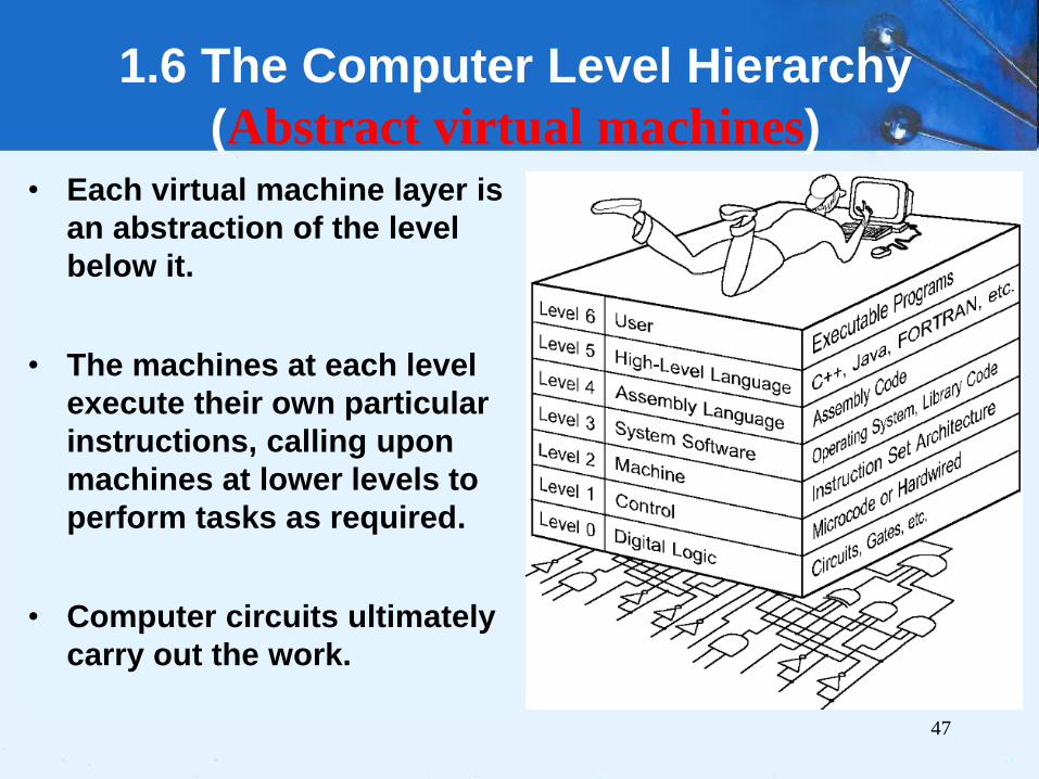
• Each virtual machine layer is

an abstraction of the level

below it.

• The machines at each level

execute their own particular

instructions, calling upon

machines at lower levels to

perform tasks as required.

• Computer circuits ultimately

carry out the work.


(Abstract virtual machines)

48

• Level 6: The User Level

– Program execution and user interface level.

– The level with which we are most familiar.

• Level 5: High-Level Language Level

– The level with which we interact when we write

programs in languages such as C, Pascal, Lisp, and

Java.


49

• Level 4: Assembly Language Level

– Acts upon assembly language produced from

Level 5, as well as instructions programmed

directly at this level.

• Level 3: System Software Level

– Controls executing processes on the system.

– Protects system resources.

– Assembly language instructions often pass

through Level 3 without modification.


50

• Level 2: Machine Level

– Also known as the Instruction Set Architecture

(ISA) Level.

– Consists of instructions that are particular to the

architecture of the machine.

– Programs written in machine language need no

compilers, interpreters, or assemblers.


51

• Level 1: Control Level

– A control unit decodes and executes instructions

and moves data through the system.

– Control units can be microprogrammed or

hardwired.

– A microprogram is a program written in a low-

level language that is implemented by the

hardware.

– Hardwired control units consist of hardware that

directly executes machine instructions.


52

• Level 0: Digital Logic Level

– This level is where we find digital circuits

(the chips).

– Digital circuits consist of gates and wires.

– These components implement the

mathematical logic of all other levels.


1.7 CLOUD COMPUTING

(virtual computing platform)

53

SaaS

PaaS

IaaS

1.7 CLOUD COMPUTING

• The “computer” and “storage” appear to

the user as a single entity in the Cloud but

usually span several physical servers.

• It presents a virtual machine to the user.

• At the top of the computer hierarchy, where

we have executable programs, a Cloud

provider might offer an entire application

over the Internet, with no components

installed locally. This is called Software as

a Service, or SaaS.

54

1.7 CLOUD COMPUTING

• Consumer that desire to have more control

over their applications, or that need

applications for which SaaS is unavailable,

• might instead opt to deploy their own

applications on a Cloud-hosted environment

called Platform as a Service, or PaaS.

55

1.7 CLOUD COMPUTING

• If a company’s main business is software

development. PaaS is not a good fit in situations

where rapid configuration changes are required.

• Indeed, in any company where staff is capable of

managing operating system and database

software, the Infrastructure as a Service (IaaS)

• PaaS and IaaS provide elasticity: the ability to

add and remove resources based on demand. A

customer pays for only as much infrastructure as

is needed. 56

1.7 CLOUD COMPUTING

• Cloud model charges fees in proportion to

the resources consumed.

• These resources include communications

bandwidth, processor cycles, and storage.

• Thus, to save money, application programs

should be designed to reduce trips over the

network, economize machine cycles, and

minimize bytes of storage.

57

58

• On the ENIAC, all programming was done at

the digital logic level. Programming the

computer involved moving plugs and wires.

• A different hardware configuration was needed

to solve every unique problem type.

1.8 The von Neumann Model

Configuring the ENIAC to solve a “simple” problem

required many days labor by skilled technicians.

59

• The invention of stored program

computers has been ascribed to a

mathematician, John von Neumann,

who was a contemporary of Mauchley

and Eckert.

• Stored-program computers have

become known as von Neumann

Architecture systems.


60


• Today’s stored-program computers have the following characteristics:

– Three hardware systems: • A central processing unit (CPU)

• A main memory system

• An I/O system

– The capacity to carry out sequential instruction processing.

– A single data path between the CPU and main memory.

• This single path is known as the von Neumann bottleneck.

61


• This is a general depiction of a von Neumann system:

• These computers employ a fetch-decode-execute cycle to run programs as follows . . .

62


• The control unit fetches the next instruction from memory using the program counter to determine where the instruction is located.

63


• The instruction is decoded into a language that the ALU can understand.

64


• Any data operands required to execute the instruction are fetched from memory and placed into registers within the CPU.

65


• The ALU executes the instruction and places results in registers or memory.

1.8 The von Neumann Model Modified von Neumann Architecture, Adding a System Bus.

• Data bus moves data from RAM to CPU registers (and vice versa).

• Address bus holds address of the data that the data bus is currently

accessing.

• Control bus carries the necessary control signals that specify how

the information transfer is to take place. 66

67

• Conventional stored-program computers have undergone many incremental improvements over the years.

• These improvements include adding specialized buses, floating-point units, and cache memories, to name only a few.

• But enormous improvements in computational power require departure from the classic von Neumann architecture.

• Adding processors is one approach.

1.9 Non-von Neumann Models

68

• In the late 1960s, high-performance computer

systems were equipped with dual processors to

increase computational throughput.

• In the 1970s supercomputer systems were

introduced with 32 processors.

• Supercomputers with 1,000 processors were

built in the 1980s.

• In 1999, IBM announced its Blue Gene system

containing over 1 million processors.


69

• Parallel processing is only one

method of providing increased

computational power.

• DNA computers, quantum computers,

and dataflow systems. At this point, it is

unclear whether any of these systems

will provide the basis for the next

generation of computers.


70

Leonard Adleman is often called the inventor

of DNA computers. His article in a 1994 issue

of the journal Science outlined how to use

DNA to solve a well-known mathematical

problem, called the "traveling salesman"

problem. The goal of the problem is to find the

shortest route between a number of cities,

going through each city only once. As you add

more cities to the problem, the problem

becomes more difficult. Adleman chose to find

the shortest route between seven cities. DNA

computing is still in its infancy.


1.10 PARALLEL PROCESSORS AND

PARALLEL COMPUTING

• Multicore architectures are parallel

processing machines that allow for multiple

processing units (often called cores) on a

single chip.

• What is a core?

• Each processing unit has its own ALU and

set of registers, but all processors share

memory and some other resources.

71


PARALLEL COMPUTING

• Multiple cores, or multicore, provides the

potential to increase performance without

increasing the clock rate.

• With Dual core, caches became larger,

– it made performance sense to create two and

then three levels of cache on a chip,

– with the first-level cache dedicated to an

individual processor.

– and levels two and three being shared by all the

processors. 72

1.10 PARALLEL PROCESSORS

Intel Core Duo

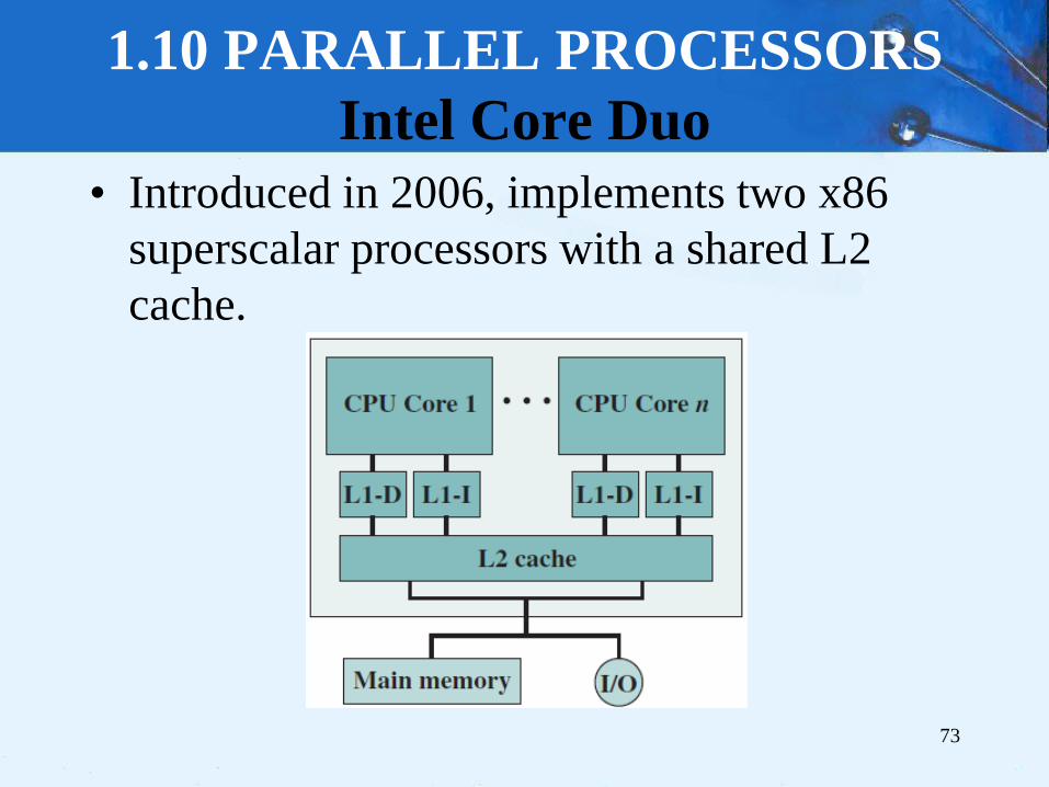
• Introduced in 2006, implements two x86

superscalar processors with a shared L2

cache.

73


Intel Core Duo Block Diagram

74

• Each core has L1 cache: L1-I=32

kB and L1-D 32-kB.

• Each core has an independent

thermal control unit, especially

for laptop and mobile systems.

• Advanced Programmable

Interrupt Controller (APIC).

• power management logic, for

reducing power consumption,

increasing battery life for mobile

platforms, such as laptops.

• Chip includes a shared 2-MB L2

cache.

• Bus interface connects to the

external bus.


Intel Core i7-990X Block Diagram

• Introduced in November

of 2008,

• implements four x86

Simultaneous

multithreading (SMT)

processors,

• each with a dedicated L2

cache, and with a shared

L3 cache

75


PARALLEL COMPUTING

• “Dual core” is

different from “dual

processor.”

• Dual-processor

machines, for

example, have two

processors, but each

processor plugs into

the motherboard

separately. 76


PARALLEL COMPUTING

• Multiple cores does not mean it will run your programs

more quickly.

• Application programs (including OS) must be written to

take advantage of multiple processing units.

• Multicore computers are very useful for multitasking—

– Ex: you may be reading email, listening to music, browsing

the Web, and burning a DVD all at the same time.

– These “multiple tasks” can be assigned to different processors

and carried out in parallel, provided the operating system is

able to manipulate many tasks at once.

77


PARALLEL COMPUTING

• Multithreading can also increase the performance

of any application with inherent parallelism.

• Programs are divided into threads, which can be

thought of as mini-processes.

• Ex: Web browser is multithreaded;

– one thread can download text,

– while each image is controlled and downloaded by a

separate thread.

• If an application is multithreaded, separate threads

can run in parallel on different processing units. 78


PARALLEL COMPUTING

• If parallel machines and other non–von Neumann

architectures give such huge increases in processing speed

and power, why isn’t everyone using them everywhere?

• The answer lies in their programmability.

• Advances in operating systems that can utilize multiple

cores have put these chips in laptops and desktops that we

can buy today;

– However, true multiprocessor programming is more complex

than both uniprocessor and multicore programming and requires

people to think about problems in a different way, using new

algorithms and programming tools.

79

80

Transputer

IMSB008 base platform with IMSB419 and IMSB404 modules

mounted

Cr: https://en.wikipedia.org/wiki/Transputer

81

• This chapter has given you an overview

of the subject of computer architecture.

Conclusion

82

End of Chapter 1

Documents

“Computing is not about computers anymore. It is aboutstaff.cs.psu.ac.th/sathit/ComOr/Ch1Intro.pdf · •Peta- (P) = 1 quadrillion ... • Hertz = clock cycles per second (frequency)