Computers and the Trade Deficit: The Case of the Falling

This PDF is a selection from an out-of-print volume from the National Bureauof Economic Research

Volume Title: International Economic Transactions: Issues in Measurementand Empirical Research

Volume Author/Editor: Peter Hooper and J. David Richardson, editors

Volume Publisher: University of Chicago Press

Volume ISBN: 0-226-35135-1

Volume URL: http://www.nber.org/books/hoop91-1

Conference Date: November 3-4, 1989

Publication Date: January 1991

Chapter Title: Computers and the Trade Deficit: The Case of the Falling Prices

Chapter Author: Ellen E. Meade

Chapter URL: http://www.nber.org/chapters/c8427

Chapter pages in book: (p. 61 - 88)

2 Computers and the Trade Deficit The Case of the Falling Prices

Ellen E. Meade

2.1 Introduction

Over the past two decades, technological advances in the computer industry have been enormous. During the 1970s, running a computer program involved a number of cumbersome tasks: typing out computer cards at a key- punch machine, submitting the job by processing the deck of cards through a card reader, and waiting for written output from a printer. Today, the same computer program can be run in a variety of ways, all of which are extremely simple, efficient, and affordable. And the reduction in the size of computers, from the gigantic mainframe to the portable personal computer, has made international trade in these goods more important. Today, we benefit not only from advances in the domestic computer market, but from technological gains in overseas markets as well.

For economists observing the rapid development in the computer market, a couple of important questions arise. First, how do we measure the advancement in the computer industry in a meaningful way? Ideally, we would like to measure a number of factors: for instance, the availability of new products, the apparent decline in the relative price of computer power, and the resultant increase in our productivity. Second, as computers become an increasingly important product in international markets, how can we best predict future developments? If we think that technological advances in the computer industry may be expected to continue as they have recently, then we want to treat

Ellen E. Meade is a staff economist in the Division of International Finance, Federal Reserve Board of Governors.

Thanks to NBER conference participants, Robert B. Kahn, David H. Howard, and William R. Melick for detailed comments and suggestions. Lucia Foster provided excellent research assist- ance and Virginia Carper provided graphics expertise. The views expressed in this paper are the author’s and do not necessarily coincide with the views of the Federal Reserve Board or other members of its staff.

61

62 Ellen E. Meade

this industry separately when formulating predictions, because its behavior differs so much from other industries.

This paper addresses both of these questions. The proper measurement of prices of domestic computers has been the subject of a number of recent studies (including Cartwright 1986, Cole et al. 1986, Dulberger 1989, and Gor- don 1989). The Bureau of Economic Analysis (BEA) has modified its traditional approach to price measurement with techniques to incorporate adjustment for quality change, in order to capture the developments in the computer market more comprehensively. A hedonic price index was devel- oped to measure prices of domestic computing equipment; the same index is now being used to deflate exports and imports of computers as well. Section 2.2 gives a detailed discussion of the construction of the BEA index for computer prices and the potential problems involved in using a domestic index to deflate other categories of spending.

When the BEA index is used to deflate the value of traded computers, the quantity of exported and imported computers shows tremendous growth over the last decade. These data are reviewed in section 2.3. Empirical trade models have focused on aggregate historical relationships and have not accounted for developments in the computer industry separately. The paper examines the extent to which separate treatment of computers is warranted, by comparing a conventional trade model with a model that disaggregates exports and imports of computers from other trade flows. The models are outlined in section 2.4. The comparison of models in section 2.5 is based on parameter estimates as well as on the forecasting ability in and out of sample.

2.2 Measurement of Computer Prices

2.2.1 Limitations of the Traditional Matched-Model Approach

A traditional procedure for the measurement of prices is the “matched- model” approach. A matched-model index records the price for an identical product (produced by identical technology) across two different time periods. I

Products that are available in the first period but discontinued in the second period, as well as new products that become available in the second period but are not produced in the first period, are excluded from the sample, since prices of these products are not available for both time periods. Generally, this does not present a problem for the construction of the index, if the price movements of the products included in the index accurately reflect the movement of prices omitted from the index. In order to form the price index across a number of

1. The formula for a price index (I) at time f. with a base period of t - I is:

I, , ,- I = c Pn.,QJ c P#,,- ,Pa., where the index is constructed over i types of the product. P,,, represents the price of product i at time r . Q,, is the quantity of i purchased at time t . The index is used to deflate current dollar figures (a Paasche index).

63 Computers and the Trade Deficit

time periods, these adjacent-year matched-model indexes are linked together multiplicatively in a “chain” index.2

The discontinuation of outdated products and the introduction of new products may pose a problem for price measurement, however, if technological advancement in the industry is particularly rapid. This concept can best be explained by way of example: good x is produced in both the first and second periods; its price is sampled for the matched-model index. Good y, identical in characteristics to x but produced with a newer technology, is introduced in the second period. Because it is produced with a more efficient technology, good y is less expensive than good x . In the long run, both good x and good y should sell for the same price, since the products are identical. But in the short run, until equilibrium is established in the market, there will be a price differential. Since the matched-model index only includes the price of good x, it tends to overstate the level of prices. In some studies, this phenomenon is termed “technologically-induced disequilibrium,” since it is the lack of instan- taneous adjustment to a new equilibrium that causes the traditional matched- model index to misstate true price changes3 (see Cole et al. 1986, Triplett 1986, and Dulberger 1989, for further discussion of the need for hedonic methods). Obviously, the more rapid is the technological advancement in an industry (implying frequent reductions in price and many new products), the greater is the concern about using the matched-model approach to capture price change.

2.2 .2 The Hedonic Approach

Advances in the computer market since the early 1970s have generated in- credible gains in efficiency and a broad array of newly available products. The concern about “technologically-induced disequilibrium” has prompted BEA to augment the traditional matched-model approach to the measurement of computer prices with techniques that adjust for improvement in quality. In essence, these techniques generate estimates for missing prices (in the above example, the price of product y in the first period), so that the matched-model index is formulated over a complete sample of prices. The method used to generate the missing prices is a hedonic regression that relates the behavior of product prices (the dependent variable) to a time dummy, important product characteristics, and a measure of technology (the explanatory variable^).^ A

2 . Using the notation defined in footnote 1, the index for the entire period can be written as:

I , , = I , , x I , , x , . . . , x I , _ , ,

3. The difference between the traditional matched-model index and an index that accounts for quality improvement is quite substantial for several components of computers. Cole et al. (1986) compare a matched-model index with three different hedonic indexes for four computer components (processors, disk drives, printers, and general purpose displays). For each component, the hedonic indexes declined twice as much or more on average than the matched-model index.

4. It is the time dummy that actually captures price movements, once characteristics and technology are controlled for.

64 Ellen E. Meade

number of authors have investigated the appropriate specification of hedonic regressions for computer processors and parts, including the choice of functional form, product characteristics included, and estimation restrictions (see Cole et al. 1986, Dulberger 1989, and Gordon 1989).

2.2.3

Underlying the hedonic approach is the assumption that the price of a product reflects the characteristics bundled in that product. If the hedonic regression adequately controls for changes in the embodied characteristics, then residual price change is the result of technological improvement. Implemen- tation of hedonic techniques for computers requires an appropriate definition of both the product and the product characteristics. BEA defines the computer in terms of individual pieces of equipment and constructs price indexes for each component ~eparately.~ While the running of a job on a computer may require several pieces of computer equipment acting in sequence, the individual pieces possess different characteristics. Furthermore, although most computer purchases are of a system of components, only the individual prices are observed (and discounting is common for a system purchase). For these rea- sons, hedonic techniques are applied to the individual computer components rather than to the computer system as a whole. The components measured in the BEA index include computer processors, disk drives, printers, general purpose displays (terminals), and personal computers.6

In addition, adequate coverage of the characteristics that determine the value of each component is critical to the success of the hedonic technique. The IBM Corporation, in developing the hedonic regressions, selected the relevant characteristics for four of the components: for computer processors, speed of execution of a set of instructions and memory capacity; for disk drives, memory capacity and speed of transfer between the drive and the main memory; for printers, speed, resolution of print, and number of fonts available; and for terminals, screen capacity, resolution, number of screen colors, and number of programmable function keys.’

An augmented matched-model index is constructed for each of the four components, using predictions from the hedonic regressions to fill in missing prices. That is, the hedonic regression predicts what the price of the component would have been, given its characteristics and technology, if had it been

Product Coverage and Construction of the Hedonic Index

5 . The initial research and development of the computer index was provided by the 1BM Cor- poration and is documented in Cole et al. (1986). Since that time, BEA has altered the original index relatively little. BEA began using this adjusted matched-model index to deflate computer purchases in the GNP accounts in 1985 and has revised the historical data back to 1969 to incorporate this index.

6. Tape drives were covered in the index through 1983 but were excluded thereafter, reflecting their declining importance. Prices of tape drives are assumed to be represented by the average change in the prices of other components.

7. As Gordon (1989) points out, there are a number of critical attributes excluded from hedonic studies on computers. These are software maintenance, engineering support, and manufacturer’s reputation-characteristics which are virtually impossible to measure.


available at a particular date. The price measure for personal computers does not involve hedonics; it is a traditional matched-model index covering price changes for IBM products and personal computers from several other manufacturers. The aggregate index for computers is a weighted average of the augmented matched-model indexes for computer processors, disk drives, printers, and displays, and the unaugmented matched-model index for personal computers. The weights used to construct the index are shares of each component in the shipments of domestic manufacturers.

2.2.4 Caveats

Several comments are in order regarding the construction and the useful- ness of the BEA price index for computers. First, if the technological development in the personal computer market has been as rapid as in the market for other computer products, then the estimation of PC prices from a traditional matched-model index will bias the price upward.* Second, for all of the components in the BEA index, the data on prices were for list prices rather than for actual transactions prices. Discounting is a common practice in the computer industry, especially for the purchase of a system of components. To the extent that different components are discounted by different margins, this adds an additional source of bias.

Third, several recent studies have investigated the role of this computer price index in the measurement of productivity (see Baily and Gordon 1988 and Denison 1989). These studies consider whether the use of this computer deflator in the GNP accounts has biased measures of productivity and output and perhaps misattributed the gain in computer power (for the BEA opinion on this subject, see Young 1989). While this line of research is timely and important, it is beyond the scope of the study here.

Fourth, very few countries currently employ hedonic techniques for the measurement of computer prices. Based on the author’s survey, only Canada and Australia use a hedonic price index. Both of these countries obtain the component price indexes from BEA, adjust for bilateral exchange-rate changes vis-a-vis the dollar, and use own-country weights to form the aggregate index. Japan measures prices of domestic and traded computers with a unit value index, derived from value and quantity data. While economists with the Economic Planning Agency in Japan acknowledge the need for hedonic techniques, they feel that these techniques are too complicated to pursue. The United Kingdom follows a traditional matched-model p ro~edure .~ Clearly, in- dicators of international price competitiveness may be biased by the lack of standardization in the measurement of computer prices.

A final concern involves the broad use of this computer price index in the

8. Another index for PC prices was described in Gordon (1987). Like the BEA index, the Gordon index was constructed as a traditional matched-model index.

9. These survey results are broadly consistent with those of an OECD survey of 13 member countries in 1985. At that time, only the United States and Canada employed hedonic techniques.

66 Ellen E. Meade

GNP accounts. The components in the index reflect prices for the domestic market, as well as exported and imported computers; the aggregate index is formed using weights in domestic shipments. While the index is a hybrid, it seems most appropriate for the deflation of the computer portion of producers' durable equipment. However, the price is also used to deflate exports and imports of computers.I0 Using this index to deflate exports and imports of computers will be unbiased only if: (i) export and import prices for the individual computer components are identical to domestic prices;" and (ii) the mix of each of the components in exports and imports is identical to that in domestic shipments.

To test the first of these two conditions, the research staff at IBM has gath- ered information on the prices of the individual components. These data re- veal that, with the exception of printers, prices of domestic components do not differ systematically from the prices of traded components. Imported printers, however, exhibit systematic price differentials relative to domestic printers. This is because the United States has tended to produce and export system printers whose prices have fallen less rapidly than the prices of imported PC printers. Regarding the second condition, data for 1988 suggest that the component mix of exports is similar to that of domestic shipments. Imports, on the other hand, appear to have a lower share of computer processors and a higher share of printers and other peripheral equipment than found in domestic shipments.I* Evidence on the above two conditions suggests: (i) that the domestic computer price index may be a relatively unbiased measure of the prices of exported computers, but be an inappropriate measure of the prices of imported computers; (ii) that if the prices of imported computer components and the mix of the components in imports were adequately measured, the prices of imported computers would likely be found to have fallen more rapidly than the prices of domestic and exported computers.

2.3 Computer Prices and International 'Ikade

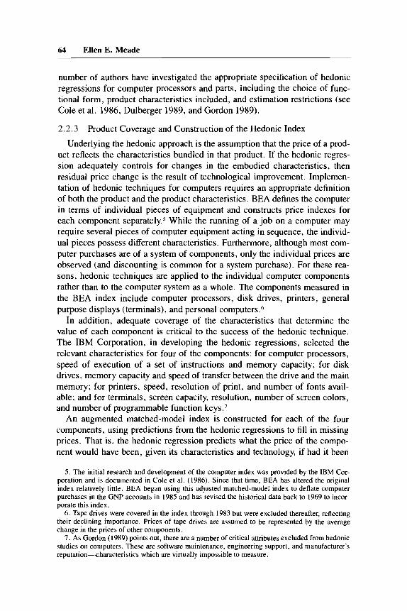
The BEA adjusted matched-model (or hedonic) index for computers used in the deflation of exports and imports is shown in figure 2.1 and table 2.1 below. According to this index, computer prices have declined more than 14

10. The price index is also used to deflate government expenditure on computers (federal as well as state and local). Currently, consumer purchases of computers are deflated using the matched-model index for PCs.

The domestic price index for office, computing, and accounting machinery (OCAM) is used to deflate exports and imports of business and office machines through 1984. From 1985 on, exports and imports of computers, peripherals, and parts are deflated using the computer index. The OCAM index is a composite of BEA's computer index, and the PPI for office and accounting machinery (excluding computers).

1 1. This bias will contaminate not only the deflation of traded computers, but the deflation of domestic purchases as well.

12. This is a preliminary finding of a project to construct component shares for exports and imports and then to use these shares to compute price indexes for computer exports and imports.


Index, 1982-100

1980 1981 1982 1983 1984 1985 1986 1987 1988 1989

Fig. 2.1 BEA index of computer prices

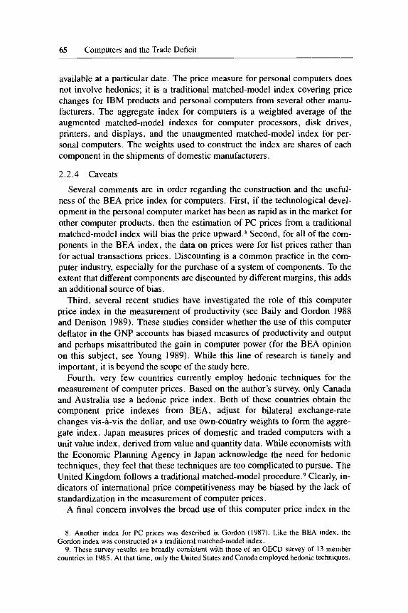
Table 2.1 Measures of Computer Prices

160

140

120

100

80

60

40

20

BE& B LS-Export BLS-Import

Level Changeb Level Changeb Level Changeh ~ ~~~~

1982:Q4 1983:Q4 I984:Q4 1985:Q4 1986:Q4 1987:Q4 1988:Q4 1989:Q4

~ ~~~

98.5 -4.6 76.4 - 22.4 65.5 - 14.3 46.8 -28.5 41.7 - 10.9 35.2 - 15.6 34 8 -1 .1 31.1 - 10.6

n.a. n.a.

102.4 n.a. 99. I -3.2 98.0 - 1.1 95.0 -3.1 95.5 0.5 93.6 - 2.0

n.a. n.a.

100.7 n.a. 102.4 1.7 104.1 1.7 112.2 7.8 111.3 - 0.8 110. I - 1.1

"BEA uses the same price index to deflate exports and imports. bPercentage change, computed on a 44-44 basis.

percent per year on average since 1982 (fourth quarter to fourth quarter), and by the end of 1989 were almost 70 percent below their 1982 le~e1 . I~ These price movements differ markedly from the rate of price change in an altema- tive measure of computer prices constructed by the Bureau of Labor Statistics. The BLS index for the prices of exported computers has declined modestly since the end of 1984 (the data are not available prior to that time), while the

13. Measured from the beginning of the hedonic index in 1969 through 1988, the computer price declined almost 7 percent per year on average.

68 Ellen E. Meade

index of import prices has actually increased over the same period. The difference between the BEA price and the alternative BLS measures can be traced to the construction of the indexes; the BLS prices are traditional matched- model indexes, not adjusted to capture the effects of discontinued models or newly introduced products. It is interesting to note that the BLS price index for exports of computers differs significantly from the index for imports, call- ing into question the BEA practice of imposing identical prices.

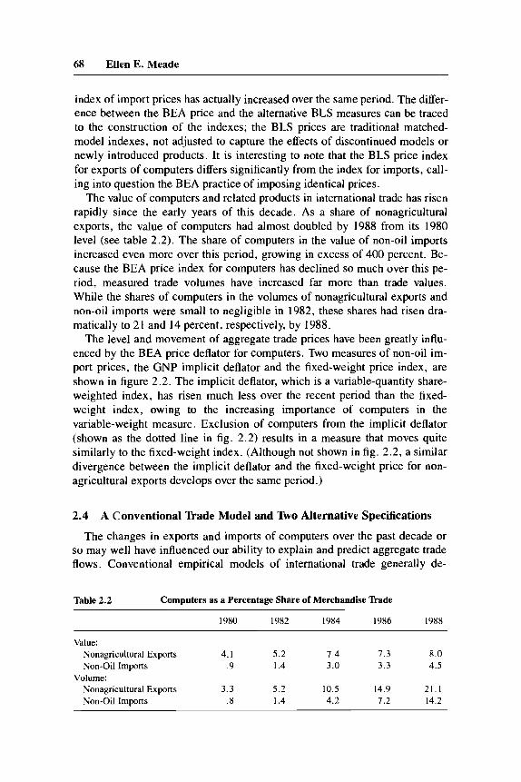
The value of computers and related products in international trade has risen rapidly since the early years of this decade. As a share of nonagricultural exports, the value of computers had almost doubled by 1988 from its 1980 level (see table 2.2). The share of computers in the value of non-oil imports increased even more over this period, growing in excess of 400 percent. Be- cause the BEA price index for computers has declined so much over this period, measured trade volumes have increased far more than trade values. While the shares of computers in the volumes of nonagricultural exports and non-oil imports were small to negligible in 1982, these shares had risen dra- matically to 21 and 14 percent, respectively, by 1988.

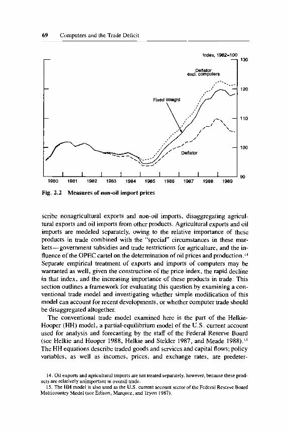
The level and movement of aggregate trade prices have been greatly influenced by the BEA price deflator for computers. Two measures of non-oil import prices, the GNP implicit deflator and the fixed-weight price index, are shown in figure 2.2. The implicit deflator, which is a variable-quantity share- weighted index, has risen much less over the recent period than the fixed- weight index, owing to the increasing importance of computers in the variable-weight measure. Exclusion of computers from the implicit deflator (shown as the dotted line in fig. 2.2) results in a measure that moves quite similarly to the fixed-weight index. (Although not shown in fig. 2.2, a similar divergence between the implicit deflator and the fixed-weight price for nonagricultural exports develops over the same period.)

2.4 A Conventional Rade Model and W o Alternative Specifications

The changes in exports and imports of computers over the past decade or so may well have influenced our ability to explain and predict aggregate trade flows. Conventional empirical models of international trade generally de-

Table 2.2 Computers as a Percentage Share of Merchandise Trade

1980 1982 I984 1986 1988 ~~~~~~ ~ ~~~ ~~

Value: Nonagricultural Exports 4. I 5.2 1.4 1.3 8.0 Non-Oil Imports .9 1.4 3.0 3.3 4.5

Nonagricultural Exports 3.3 5.2 10.5 14.9 21.1 Volume:

Non-Oil Imports .8 I .4 4.2 1.2 14.2


Index. 1982-1 00 130

120

110

loo

90 1980 1981 1982 1983 1984 1985 1986 1987 1988 1989

Fig. 2.2 Measures of non-oil import prices

scribe nonagricultural exports and non-oil imports, disaggregating agricultural exports and oil imports from other products. Agricultural exports and oil imports are modeled separately, owing to the relative importance of these products in trade combined with the “special” circumstances in these markets-government subsidies and trade restrictions for agriculture, and the influence of the OPEC cartel on the determination of oil prices and production. l4 Separate empirical treatment of exports and imports of computers may be warranted as well, given the construction of the price index, the rapid decline in that index, and the increasing importance of these products in trade. This section outlines a framework for evaluating this question by examining a conventional trade model and investigating whether simple modification of this model can account for recent developments, or whether computer trade should be disaggregated altogether.

The conventional trade model examined here is the part of the Helkie- Hooper (HH) model, a partial-equilibrium model of the U.S. current account used for analysis and forecasting by the staff of the Federal Reserve Board (see Helkie and Hooper 1988, Helkie and Stekler 1987, and Meade 1988).15 The HH equations describe traded goods and services and capital flows; policy variables, as well as incomes, prices, and exchange rates, are predeter-

14. Oil exports and agricultural imports are not treated separately, however, because these prod-

15. The HH model is also used as the U.S. current account sector of the Federal Reserve Board ucts are relatively unimportant in overall trade.

Multicountry Model (see Edison, Marquez, and Tryon 1987).

70 Ellen E. Meade

mined. l 6 The key equations for merchandise trade are the volumes and prices of nonagricultural exports and non-oil imports-the determinants of the partial trade balance.

Quantities of traded goods depend on real income and relative prices, while prices of traded goods depend on input prices, exchange rates, and the prices of competing products. In general, the form for the determinants of the partial trade balance in the HH model can be written as follows:

(1) x = fly,, (P, . E/P,)I

( 2 ) M = f [ Y , (TR . Pm/P)]

(3) P, = f[pw, (P,/E)I

(4)

( 5 )

Pm = f [P,, E9 Pcmdl

PTB = X ' PI - M . P,

where X = nonagricultural export quantity; M = non-oil import quantity; E = exchange rate (units of foreign currency per dollar); P(P,) = domestic (foreign) prices; Pn = producer price for nonagricultural exports; P, (P,) = implicit deflator for nonagricultural exports (non-oil imports); Pcmd = price of non-oil commodities; Y = U.S. real GNP; Y, = index of weighted average rest-of-world real GNP; TR = index of tariff rates; and PTB = partial trade balance. In the HH model, several other variables augment the equations. A dummy

variable to measure dock strikes appears in both trade volume equations (see Isard 1975). In the equation for non-oil import volume, a variable measuring capacity utilization abroad relative to capacity utilization in the United States captures cyclical variation (a cyclical measure in the export volume equation was dropped due to statistical insignificance). A relative secular supply variable (the ratio of measures of U.S. capital stock to foreign capital stock) appears in both trade volume equations as a proxy for supply-induced shifts in production (see Helkie and Hooper 1988, p. 20).

The HH formulation measures the prices of traded products with implicit deflators. As discussed above, price indexes in which the share of computers is variable have behaved quite differently over the recent period from indexes

16. A typical criticism of this partial-equilibrium framework is that different policies have different effects on incomes, prices, and exchange rates. In this sort of model, incomes, prices, and exchange rates are predetermined, and policy has no explicit role. Thus, a particular change in the predetermined variables has an identical effect on trade flows, regardless of the underlying policy. Essentially, the parameter estimates measure the responsiveness of trade flows to changes in predetermined variables, given the average mix of policies that generated the historical data.


in which the weight given to computers is fixed. Because of the rapidly chang- ing role of computers between the estimation period and the postsample period, equations explaining the implicit deflator have predicted poorly out of sample. A proposed improvement to the conventional specification is to base the price equations on fixed-weight measures. In a modified HH formulation (termed the HHFW model), the behavioral price equations (3) and (4) are reestimated with fixed-weight price indexes in place of the deflators; bridge equations are then used to relate the fixed-weight price indexes to the implicit deflators, as follows:”

where P, (PF,,,) = fixed-weight price index for nonagricultural exports (non- oil imports); and Ll(.) defines the first-order lag operator. Equations (l), (2), and ( 5 ) , which determine the quantity of nonagricultural exports, the quantity of non-oil imports, and the partial trade balance, respectively, remain unchanged.

A second, more fundamental, alternative to the original HH specification involves disaggregating computers from the other elements of the partial trade balance and determining trade in computers separately. In this formulation, equations ( l ) , ( 2 ) , (3 ) , and (4) represent the volumes and prices of nonagricultural exports and non-oil imports excluding computers. The computer (HHC) model is closed by adding three equations to determine the volume and price of computer exports and imports.I9 The initial specification tested for the quantity of computer exports and imports includes an income term, as well as two relative price measures. The first relative price term captures shifts in aggregate trade prices versus domestic prices; the second relative price term measures the shift of prices within nonagricultural exports and non-oil imports between computers and other products:

(9) M< = f [y , (TR.P,,,IP). RP,,rcl

where X c = computer export quantity; Mc = computer import quantity; and RPrC (RP,,) = the price of computers relative to the implicit deflator for nonagricultural exports (non-oil imports) excluding computers.

17. I t is still necessary to produce an estimate for the implicit deflator, as this measure is used to form the relative price term in equations (1) and (2) and to compute the partial trade balance in equation (5).

18. Thus, the endogenous variables, X . M , P,, and Pm must be redefined to exclude computers. 19. Recall that the same price index is used to deflate the value of exports and imports. Thus,

only one price equation is necessary.

72 Ellen E. Meade

The equation for computer prices differed from the other behavioral price equations. Because the BEA index for computer prices essentially tracks price conditions in the domestic market and is adjusted further to account for changes in quality, computer prices were modeled as a time series augmented by a linear trend term to capture technological progress:

(10) P, = f[Ll(P,), TREND]

where P, = implicit deflator for computer exports and imports; and TREND = linear time trend.

2.5 Empirical Results

The proper treatment of computers in empirical trade models is evaluated by the comparison of the original Helkie-Hooper (HH) model with the two alternative specifications-the fixed-weight aggregate model (HHFW) and the model with computers disaggregated (HHC). First, we examine key parameter estimates in the HH, HHFW, and HHC models. The parameters of particular interest include the income and relative price elasticities in the trade volume equations and the sensitivity of import prices to exchange rates (the “pass-through’ coefficient). Second, we compare the forecasting ability of the components of the partial trade balance both in and out of sample using a summary error statistic (root mean square percent error). Finally, we examine the errors in the projection of the partial trade balance for each of the models.

2.5.1 Parameter Estimates

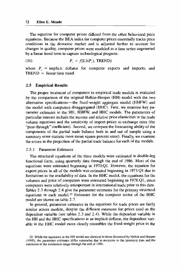
The structural equations of the three models were estimated in double-log functional form, using quarterly data through the end of 1986. Most of the equations were estimated beginning in 1970:Ql. However, the equation for export prices in all of the models was estimated beginning in 1973:Ql due to limitations in the availability of data. In the HHC model, the equations for the volumes and price of computers were estimated beginning in 1978:Q1, since computers were relatively unimportant in international trade prior to this date. Tables 2.3 through 2.6 give the parameter estimates for the primary structural equations in each model.20 Estimates for the computer sector of the HHC model are shown on table 2.7.

In general, parameter estimates in the equations for trade prices are fairly similar across models, despite the different measures for prices used as the dependent variable (see tables 2.3 and 2.4). While the dependent variable in the HH and the HHC specifications is an implicit deflator, the dependent variable in the HHC model more closely resembles the fixed-weight price in the

20. While the equations in the HH model are identical to those discussed by Helkie and Hooper (1988), the parameter estimates differ somewhat due to revisions to the historical data and the extension of the estimation range through the end of 1986.


Table 2.3 Parameter Estimates for Export Price Equations, 1973:Ql-1986:44

Model

HHa HHFWb HHC'

Dependent variable Explanatory variables

Intercept

U . S . producer price (P, , )

Foreign priced (P,)

Exchange rated (E)

Summary statistics Rho

R' S.E.R

.49 (1.35)

.89 ( I 1.69)

.05 (0.68) - .05 (0.68)

.83 (23.8 1)

.99 ,011

.93 (3.81)

.80 (15.59)

.07 (1.59) - .07 ( I .59)

.77 (1 1 .OO)

.99 ,009

.45 (1.74)

.YO ( 1 6.63)

.ox ( I .46) - .ox ( I .46)

.80 (18.68)

.99

.010

Nore: Equations are estimated in double-log form. T-statistics are in parentheses. 'Dependent variable is the implicit deflator for nonagricultural exports. bDependent variable is the fixed-weight price for nonagricultural exports. The bridge equation between the fixed-weight price and the deflator is

Log(P,) = 0.03 + 0.99 X Log(LI(P,)) + 1.10 X ALog(P,,) where L 1 ( . ) is the first-order lag operator; R2 = .99; S.E.R. = ,005; and all coefficients are highly significant. The estimation range is 1970:Ql-l986:Q4. ?Dependent variable is the deflator for nonagricultural exports excluding computers. d4-quarter polynominal distributed lag.

HHFW model (see fig. 2.1). Because of this, it would not be surprising to find that the estimated parameters in the price equations of the HHC and HHFW models were more similar to each other than to the estimates of the HH model. This is not the case, however. On the whole, the key parameter estimates in the price equations are not terribly sensitive to the alternative price variables that are employed.

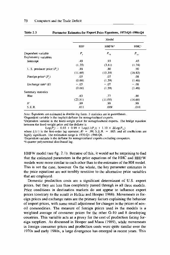
Domestic production costs are a significant determinant of U.S. export prices, but they are less than completely passed through in all three models. Price conditions in destination markets do not appear to influence export prices (contrary to the result in Helkie and Hooper 1988). Movements in foreign prices and exchange rates are the primary factors explaining the behavior of import prices, with some small adjustment for changes in the prices of non- oil commodities. The measure of foreign prices used in the models is a weighted average of consumer prices for the other G-10 and 8 developing countries. This variable acts as a proxy for the cost of production facing foreign suppliers. As discussed in Hooper and Mann (1989), while movements in foreign consumer prices and production costs were quite similar over the 1970s and early 1980s, a large divergence has emerged in recent years. This

74 Ellen E. Meade

Table 2.4 Parameter Estimates for Import Price Equations, 1970:Ql-l986:Q4

HHd HHFWb H H C

Dependent variable P"? Explanatory variables

Intercept 4.25 (12.58)

Foreign price (P,) .84 (20.85)

Exchange rated (E) -.89 (12.42)

Commodity price' (Pcd) . I8 (4.39)

Ph

4.63 (17.31)

.77 (24.15) - .81

(14.45) .08

(2.35)

P!",,,

3.93 ( I 1.89)

.85 (21.63) - .84

( I I .97) . I8

(4.54) Summary statistics

Rho

R' S.E.R

.64 .56 .63 (6.39) (5.46) (6.26)

.99 .99 .99 ,014 ,013 .014

Nore; Equations are estimated in double-log form. T-statistics are in parentheses. aDependent variable is the implicit deflator for non-oil imports. bDependent variable is the fixed-weight price for non-oil imports. The bridge equation between the fixed-weight price and the deflator is

Log(P,) = 0.99 x Log(LI(PJ) + 1.12 x ALog(P,J where LI( . ) is the first-order lag operator; RZ = .99; S.E.R. = ,007; and all coefficients are highly significant. The estimation range is 1970:QI-l986:Q4. cDependent variable is the deflator for non-oil imports excluding computers. d8-quarter polynomial distributed lag. '4-quarter polynomial distributed lag.

is an important point, to which we will return later in the discussion of simulation results.

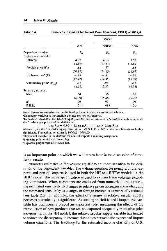
Parameter estimates in the volume equations are more sensitive to the definition of the dependent variable. The volume equation for nonagricultural exports and non-oil imports is used in both the HH and HHFW models; in the HHC model, this same specification is used to explain trade volumes excluding computers. When computers are excluded from nonagricultural exports, the estimated sensitivity to changes in relative prices increases somewhat, and the estimated sensitivity to changes in foreign income is substantially reduced (see table 2.5). In addition, the effect of changes in relative secular supply becomes statistically insignificant. According to Helkie and Hooper, this variable has traditionally played an important role, measuring the effects of the introduction of new products that are not captured adequately in relative price movements. In the HH model, the relative secular supply variable has tended to reduce the discrepancy in income elasticities between the export and import volume equations. The tendency for the estimated income elasticity of U.S.


Table 2.5 Parameter Estimates for Export Volume Equations, 1970Q1-1986:Q4

Model

HH, H H W HHCb


Intercept

Foreign income (V,)

Relative price‘

Relative supply (RSUP)d

Dock strike


R2 S.E.R

X

-4.85 (7.47) 2.04

(6.86) - .86 (7.57) 1.12

(2.25) .83

(7.01)

.61 (7.1 I )

t 99 .027

4.12 (5.01) 1.25

(8.82) - .99 (9.46)

I .20 (0 I20)

.83 (7.01)

.68 (7.75)

.98 ,027

Noret Equations are estimated in double-log form. T-statistics are in parentheses. ’Dependent variable is the volume of nonagricultural exports and is identical in models HH and HHFW bDependent variable is the volume of nonagricultural exports excluding computers. cThe relative price in the HH and HHFW models is the nonagricultural export deflator relative to foreign consumer prices in dollar terms; in the HHC model, the relative price is the deflator for nonagricultural exports excluding computers relative to foreign prices in dollars. 8-quarter polynomial distributed lag. dRatio of the capital stock in the U.S. relative to foreign countries.

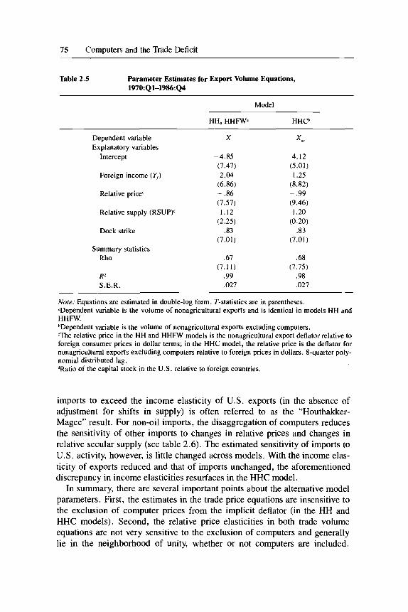
imports to exceed the income elasticity of U.S. exports (in the absence of adjustment for shifts in supply) is often referred to as the “Houthakker- Magee” result. For non-oil imports, the disaggregation of computers reduces the sensitivity of other imports to changes in relative prices and changes in relative secular supply (see table 2.6). The estimated sensitivity of imports to U.S. activity, however, is little changed across models. With the income elasticity of exports reduced and that of imports unchanged, the aforementioned discrepancy in income elasticities resurfaces in the HHC model.

In summary, there are several important points about the alternative model parameters. First, the estimates in the trade price equations are insensitive to the exclusion of computer prices from the implicit deflator (in the HH and HHC models). Second, the relative price elasticities in both trade volume equations are not very sensitive to the exclusion of computers and generally lie in the neighborhood of unity, whether or not computers are included.

76 Ellen E. Meade

Table 2.6 Parameter Estimates for Import Volume Equations, 1970:Q1-1986:Q4

Model

HH, HHFW” HHCb


Intercept

U.S. Income (Y)

Relative price‘

Relative supply

Relative capacity‘

Dock strike


R’ S.E.R

M

. I 1 (4.21) 1.97

(2.54) - 1 . 1 1 (9.81) - .90 (2.14) - 1.28 (1.64)

.78 (4.24)

.48 (4.21)

.99 ,031

- 1.49 (.29) 2.02

(2.64) - 1.02

(8.90) - .74 ( I .83) - 1.30

( 1 .73) .79

(4.26)

.47 (4.10)

.99

.03 I

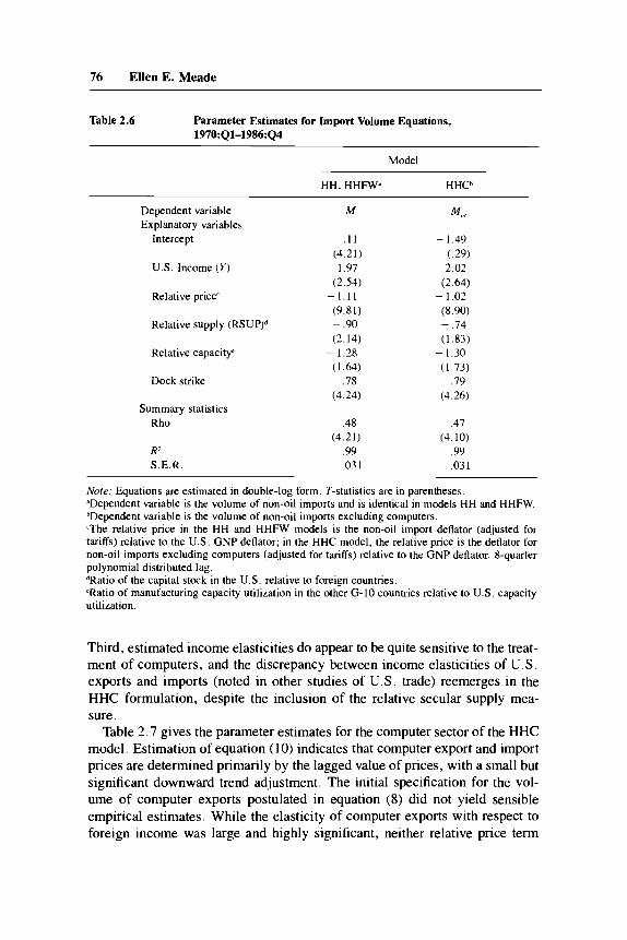
Note: Equations are estimated in double-log form. T-statistics are in parentheses. ”Dependent variable is the volume of non-oil imports and is identical in models HH and HHFW. bDependent variable is the volume of non-oil imports excluding computers. ‘The relative price in the HH and HHFW models is the non-oil import deflator (adjusted for tariffs) relative to the U.S. GNP deflator; in the HHC model, the relative price is the deflator for non-oil imports excluding computers (adjusted for tariffs) relative to the GNP deflator. %quarter polynomial distributed lag. dRatio of the capital stock in the U.S. relative to foreign countries. ‘Ratio of manufacturing capacity utilization in the other G-10 countries relative to U.S . capacity utilization.

Third, estimated income elasticities do appear to be quite sensitive to the treatment of computers, and the discrepancy between income elasticities of U.S. exports and imports (noted in other studies of U.S. trade) reemerges in the HHC formulation, despite the inclusion of the relative secular supply measure.

Table 2.7 gives the parameter estimates for the computer sector of the HHC model. Estimation of equation (10) indicates that computer export and import prices are determined primarily by the lagged value of prices, with a small but significant downward trend adjustment. The initial specification for the volume of computer exports postulated in equation (8) did not yield sensible empirical estimates. While the elasticity of computer exports with respect to foreign income was large and highly significant, neither relative price term

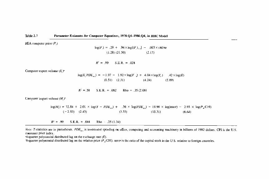
Table 2.7 Parameter Estimates for Computer Equations, 1978:Ql-l986:Q4, in HHC Model

BEA computer price (P , ) log(P<) = .29 + .94xlog[(P,)-,] - . W ~ X T R E N D

(1.28) (21.50) (2.17)

R2 = .99 S.E.R. = ,028

Computer export volume (XtY I O ~ ( X ~ / P D E , ~ , , ) = - I .97 - 1.92 X log(Y- ,) + 4.04 X log(Y,) - .42 X log(E)

(0.51) (2.31) (4.24) (2.89)

R' = ,58 S . E . R . = ,062 Rho = .35 (2.08)

Computer import volume (M,)b

lOg(M,) = 72.84 f 2.01 X l O g ( Y - PDE,") + .36 X log(PDE,,,) - 19.90 X IOg(RSUP) - 2.93 X log(PmlCPI)

( - 2.93) (2.43) (3.53) (10.31) (6.64)

R2 = .99 S.E.R. = ,044 Rho = .25(1.34)

Note: T-statistics are in parentheses. PD€,Ko is investment spending on office, computing and accounting machinery in billions of 1982 dollars, CPI is the U.S. consumer price index. "4-quarter polynomial distributed lag on the exchange rate (€). %quarter polynomial distributed lag on the relative price (P,JCPI). RSUP is the ratio of the capital stock in the U.S. relative to foreign countries.

78 Ellen E. Meade

was significantly different from zero. (When the homogeneity constraint on the relative price terms was relaxed, only the exchange rate entered the equation with a significant coefficient.) In addition, the relative secular supply variable was negatively correlated with computer exports, a result that runs counter to intuition. After considerable experimentation with alternative formulations, exports of computers were modeled as a ratio to domestic equipment spending on computers. This ratio responds positively to changes in foreign income and declines somewhat with an appreciation of the dollar. When U.S. income increases, domestic spending on computers rises relatively more than exports.

The estimated equation for the volume of computer imports is similar to the specification discussed in equation (9). All of the estimated parameters are statistically significant and of the expected sign (except for the price of computer imports relative to the price of other non-oil imports, which was dropped from the equation due to statistical insignificance). The activity variable was separated into two terms-real investment spending on office and computing machinery, and other real GNP-in order to allow for a differential response of computer imports to these two categories of income. While the estimated sensitivity of computer import volume to the relative secular supply variable and to the price of non-oil imports relative to domestic prices is of the expected sign, both elasticities are larger than expected.

In general, it was difficult to obtain sensible empirical estimates for the computer sector of the HHC model. The estimates are not particularly robust to changes in the range of estimation. Equations using time-series or error- correction techniques (instead of structural equations with a first-order auto- regressive process) would likely do better at capturing the dynamics inherent in the data.

2.5.2 Simulation Performance

Simulation results for the estimation period and for the out-of-sample period (1987:Ql-l989:Q2) were produced for the three models. These results are presented in figures 2.3 through 2.7. In order to facilitate the comparison of results across models, the analysis is presented in terms of the components of the partial trade balance. Prediction errors for the HH model equal the difference between the individual equation forecast and the actual data. For the HHFW and HHC models, the prediction errors are an aggregate of individual equation errors. For example, in the HHFW model, the prediction error for the non-oil import deflator is obtained from both the error in the structural equation explaining fixed-weight prices and the translation equation for the deflator. In the HHC model, the procedure to obtain the import deflator is even more complicated, as computer prices are predicted separately. In sum, reported prediction errors for the various components of the partial trade balance shown in figures 2.3 through 2.7 are a mix of individual equation and


- - Achrai HH

HHC

- - - - - - - HHFW -_----- - ----_

- RMS Percent Error - IN OAT

HH 3.15 8.40 HHFW 3.93 4.07

- HHC 1.55 4.61

-

.---------

1980 1981 1982 1983 1984 1985 1986

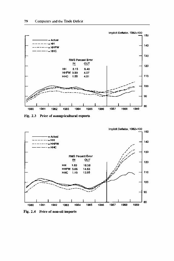
Fig. 2.3 Price of nonagricultural exports

RMS Percent Error - IN OUT

HH 1.63 18.38 HHFW 3.66 14.83 HHC 1.15 12.65

I I I I 1 I 1980 1981 1982 1983 1984 1985 1986

Fig. 2.4 Price of non-oil imports

lmpllcit Deflator. 1982-1 00 150

1987 1988 1989

140

130

120

110

100

90

80

Implicit Deflator, 1982-100

1 150 -I 140

130

120

110

100

-80 1987 1988 1989

80 Ellen E. Meade

multiple equation errors. For the three models, the simulation errors are evaluated on the basis of root mean square percent errors.21

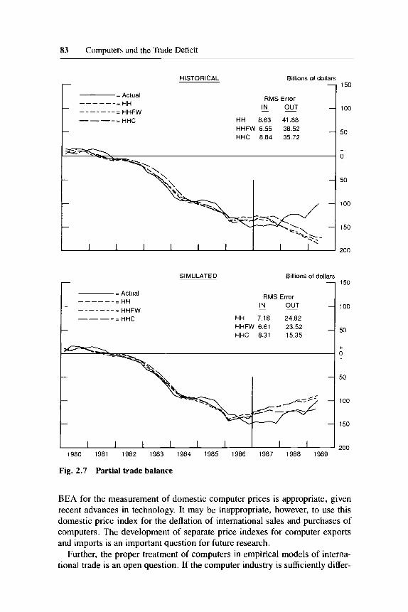
The HHC model tracks the deflators for nonagricultural exports and non-oil imports quite well over the estimation period and is more accurate than either the HH or the HHFW formulations (see fig. 2.3 and 2.4). Beyond the sample period, all of the models overpredict prices. The overpredictions are largest for the HH model; compared with the HHC model, overprediction errors in the HH model are about double the magnitude for export prices and about 50 percent larger for import prices. Despite the relative accuracy of the HHC model, errors in the prediction of the non-oil import deflator remain sizable. Much of this prediction error may result from the use of consumer prices as a proxy for foreign production costs, as discussed earlier.

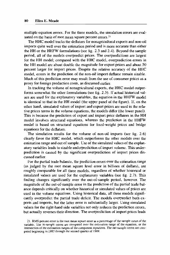
In tracking the volume of nonagricultural exports, the HHC model outperforms somewhat the other formulations (see fig. 2.5). If actual historical values are used for the explanatory variables, the equation in the HHFW model is identical to that in the HH model (the upper panel of the figure). If, on the other hand, simulated values of import and export prices are used in the relative prices terms in the volume equations, the models differ (the lower panel). This is because the prediction of export and import price deflators in the HH model involves structural equations, whereas the prediction in the HHFW model is based on structural equations for fixed-weight prices and bridge equations for the deflators.

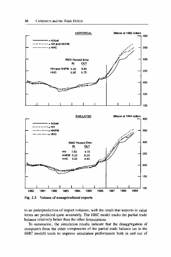
The simulation results for the volume of non-oil imports (see fig. 2.6) clearly favor the HHC model, which outperforms the other models over the estimation range and out of sample. Use of the simulated values of the explanatory variables leads to sizable underprediction of import volume. This underprediction is caused by the significant overprediction of import prices discussed earlier.

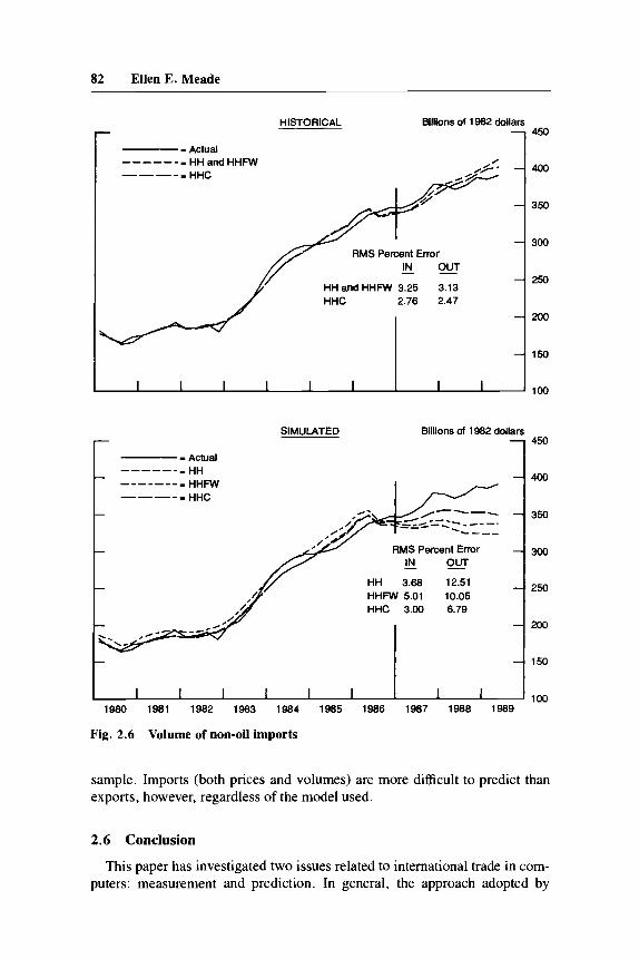
For the partial trade balance, the prediction errors over the estimation range (as judged by the root mean square level error in billions of dollars), are roughly comparable for all three models, regardless of whether historical or simulated values are used for the explanatory variables (see fig. 2.7). This finding changes significantly over the out-of-sample period, however. The magnitude of the out-of-sample error in the prediction of the partial trade balance depends critically on whether historical or simulated values of prices are used in the volume equations. Using historical data, all three models significantly overpredict the partial trade deficit. The models overpredict both exports and imports, but the latter error is substantially larger. Using simulated values for the right-hand side variables not only reduces the prediction errors, but actually reverses their direction. The overprediction of import prices leads

21. RMS percent error is the root mean square error as a percentage of the sample mean of the variable. The in-sample errors are computed over the estimation range of the equation, or the intersection of the estimation ranges of the component equations. The out-sample errors are computed beginning in 1987 through the second quarter of 1989.


- -

I I I I 1 1 I I

SIMULATED Billions of 1982 dollars

1 - Actual HH r - - - - - - HHFW HHC

-------_ ----_

RMS Percent Error - IN OAT

HH 7.53 4.73 HHFW 5.26 8.23 I HHC 3.32 4.44 .---

r,,,,,,l 1980 1981 1982 1983 1984 1985 1986 I 1987 1988 1989

400

350

300

250

200

150

100

400

350

300

250

200

150

100

Fig. 2.5 Volume of nonagricultural exports

to an underprediction of import volumes, with the result that imports in value terms are predicted quite accurately. The HHC model tracks the partial trade balance relatively better than the other formulations.

To summarize, the simulation results indicate that the disaggregation of computers from the other components of the partial trade balance (as in the HHC model) tends to improve simulation performance both in and out of

82 Ellen E. Meade

I- HISTORICAL Billions of 1982 dollars

1

7 RMS Percent Enor I - IN OUT

1 HH and HHFW 3.25 3.13 HHC 2.76 2.47

SIMULATED Billions of 1982 dollars r 1 - Actual

HH HHFW HHC

- - - - - - - - - - - - - - _---I

-

- RMS Percent Error - IN O x

HH 3.68 12.51 HHFW 5.01 10.05 HHC 3.00 6.79

-

450

400

350

300

250

200

150

loo

450

400

350

300

250

200

1 5 0

100 1980 1981 1982 1983 1984 1985 1986 1987 1988 1989

Fig. 2.6 Volume of non-oil imports

sample. Imports (both prices and volumes) are more difficult to predict than exports, however, regardless of the model used.

2.6 Conclusion

This paper has investigated two issues related to international trade in computers: measurement and prediction. In general, the approach adopted by


r HISTORICAL Billions of dollars

1

t

SIMULATED Billions of dollars - RMS Error - IN OUT

HH 7.18 24.82 HHFW 6.61 23.52 HHC 8.31 15.35

150

100

50

+ 0 -

50

100

1 50

200

1 50

100

50

+ 0 -

50

100

150

200 1980 1981 1982 1983 1984 1985 1986 1987 1988 1989

Fig. 2.7 Partial trade balance

BEA for the measurement of domestic computer prices is appropriate, given recent advances in technology. It may be inappropriate, however, to use this domestic price index for the deflation of international sales and purchases of computers. The development of separate price indexes for computer exports and imports is an important question for future research.

Further, the proper treatment of computers in empirical models of international trade is an open question. If the computer industry is sufficiently differ-

84 Ellen E. Meade

ent from other industries, separate treatment of computers in these models may be necessary to capture historical developments and predict future out- comes. The analysis in this paper suggests that the disaggregation of computers from the other components of the partial trade balance is warranted and generally leads to more accurate predictions.

References

Baily, Martin Neil, and Robert J. Gordon. 1988. The Productivity Slowdown, Mea- surement Issues, and the Explosion of Computer Power. Brookings Paper on Eco- nomic Activity 2:347-420.

Cartwright, David W. 1986. Improved Deflation of Purchases of Computers. Survey of Current Business 66 (March):7-10.

Cartwright, David W., and Scott D. Smith. 1988. Deflators for Purchases of Comput- ers in GNP: Revised and Extended Estimates, 1983-88. Survey of Current Business 68 (November):22-23.

Chow, Gregory C. 1967. Technological Change and the Demand for Computers. American Economic Review 57 (December): 1 117-30.

Cole, Rosanne, Y. C. Chen, Joan A. Barquin-Stolleman, Ellen Dulberger, Nurhan Helvacian, and James H. Hodge. 1986. Quality-Adjusted Price Indexes for Com- puter Processors and Selected Peripheral Equipment. Survey of Current Business 66 (January):4 1-50.

Denison, Edward F. 1989. Estimates of Productivity Change by Industry: An Evalua- tion and an Alternative. Washington, D.C.: The Brookings Institution.

Dion, Richard, and Jocelyn Jacob. 1988. The Dynamic Effects of Exchange Rate Changes in Canada’s Trade Balance, 1982-1987. Bank of Canada Working Paper.

Dulberger, Ellen R. 1989. The Application of a Hedonic Model to a Quality-Adjusted Price Index for Computer Processors. In Technology and Capital Formation, ed. Dale W. Jorgenson and Ralph Landau. Cambridge, Mass.: MIT Press.

Edison, Hali J., Jaime R. Marquez, and Ralph W. Tryon. 1987. The Structure and Properties of the Federal Reserve Board Multicountry Model. Economic Modelling

Gordon, Robert J. 1989. The Postwar Evolution of Computer Prices. In Technology and Capital Formation, ed. Dale W. Jorgenson and Ralph Landau. Cambridge, Mass.: MIT Press.

. 1987. The Postwar Evolution of Computer Prices. NBER Working Paper no.

4 (April): 1 15-3 15.

2227(April). Griliches. Zvi. 1964. Notes on the Measurement of Price and Ouality Changes. In

~ Models of Income Determination, NBER Studies in Income and Wialth, 61. 28. Princeton, N.J.: Princeton University Press.

Helkie, William L., and Peter Hooper. 1988. The U.S. External Deficit in the 1980s: An Empirical Analysis. In External Dejcits and the Dollar: The Pit and the Pendu- lum, ed. Ralph C . Bryant, Gerald Holtham, and Peter Hooper. Washington, D.C.: The Brookings Institution.

Helkie, William L., and Lois Stekler, 1987. Modeling Investment Income and Other Services in the U.S. International Transactions Accounts. International Finance Dis- cussion Paper no. 319. Washington, D.C.: Federal Reserve Board.

Hooper, Peter, and Catherine L. Mann. 1989. Exchange Rate Pass-through in the


1980s: The Case of U.S. Imports of Manufactures. Brookings Papers on Economic Activity 1:297-337.

Isard, Peter. 1975. Dock-Strike Adjustment Factors for Major Categories of U.S. Im- ports and Exports, 1958-74. International Finance Discussion Paper no. 60. Wash- ington, D.C.: Federal Reserve Board.

Meade, Ellen E. 1988. Exchange Rates, Adjustment, and the &Curve. Federal Reserve Bulletin 74 (October):633-44.

Rosen, Sherwin. 1974. Hedonic Prices and Implicit Markets: Product Differentiation in Pure Competition. Journal of Political Economy 82 (January-February):34-49.

Triplett, Jack E. 1986. The Economic Interpretation of Hedonic Models. Survey of Current Business 66 (January):36-40.

. 1989. Price and Technological Change in a Capital Good: A Survey of Re- search on Computers. In Technology and Capital Formation, ed. Dale W. Jorgenson and Ralph Landau. Cambridge, Mass.: MIT Press.

Young, Allan H. 1989. BEA’s Measurement of Computer Output. Survey of Current Business 69 (July): 108-15.

Comment Richard D. Haas

This is a very good paper, one in which I find much to be in agreement with, and very little to take serious issue with. Nevertheless, I do have several comments to make. They are in three parts: those centering on data and specification; those dealing with estimation issues; and those focusing on the simulation results.

Data and Specification Issues

My first concern centers on the BEA hedonic index used. The advantages of correcting the series for quality improvements are amply demonstrated. But, as Meade notes, the drawback is that one price index is used for imports, exports, and domestic production of computers. The more conventionally measured-and less desirable-BLS data shows that these are not the same and, furthermore, are diverging over time, at least for imports and exports. This is a potential source bias in the derived volumes data in the model where computers are treated separately. My question then, is whether there may be a way to extract the information from the BLS import and export data to differ- entiate the hedonic import and export indexes.

With respect to the import price equations, Meade realizes that some measure of foreign costs or prices should be used, not the CPI; but this problem is not the focus of the paper, so I will not dwell on it.

Another concern is the use of the relative price term in the fixed-weight version of the Helkie-Hooper model-the HHFW model in the text. In a pre-

Richard D. Haas is an adviser at the Economic Research Department of the International Mon- etary Fund.

86 Ellen E. Meade

liminary version of the paper, I viewed this specification as conceptually pref- erable to the conventional Helkie-Hooper model, but inferior to a version of the model in which computers are modeled separately. Now, after reviewing the estimation results, I think the fixed-weight specification can be improved. If the problem is that variable-weight deflators convey the wrong information because they give increasing weight to computers, then the problem can be minimized, but not eliminated, by using a fixed-weight deflator where the weights are fixed at a point in time when computers constituted a small portion of trade. Meade does this in the price equations in the HHFW model, but continues to use the variable-weight deflator in the relative price terms in the volume equations. In commenting on an earlier version of the present paper, I suggested first taking the fixed-weight deflators and deriving new volume data and then using the fixed-weight deflators in the relative price terms. I now have doubts about the first recommendation, but continue to think I was right on the second. In other words, I would argue that we should use the better price series-the one in which bias has been minimized and the one that shows import prices increasing between 1985 and 1987 the way we all expected them to-to explain non-oil import volumes. Of course the fixed- weight deflators would not yield the proper partial trade balances; the bridge equations estimated in the paper would still be needed for that.

With regard to the bridge equations, they are both essentially first- difference log equations with coefficients greater than one on the fixed-weight term, something I have difficulty reconciling with the plots of the two series in figure 2.2. The export transformation equation has an additional trend term of 12 percent a year that would seem to compound the problem.

Estimation Issues

Turning to estimation issues, I believe that the export price equations prob- ably should have been tested for homogeneity. It looks to me as if homogeneity would be accepted at conventional levels, and would improve the simulation characteristics of the model; a one-percent increase in the two explanatory variables, domestic costs and foreign prices, measured in dollars, would lead to a one-percent increase in export prices. Roughly similar data over approximately the same period led to an 86/14 split between the two variables when tested for (and accepted) in the IMF’s World Trade Model.

The import price equations show an exchange pass-through of 85 percent. This represents the average effect over the estimation period, as the paper points out. Whether or not there will be full or zero pass-through, depends, I should think, on whether the exchange rate was moving in response to a real shock or a monetary shock. If the former, I would look for little pass-through; if the latter, 100 percent pass-through.

As for the volume equations, Meade seems concerned that the activity elasticity in the HHC model’s nonagricultural export volume equation is too low-about one-relative to the activity elasticity in the non-oil import vol-


ume equation in the same model. I would reverse the concern and would worry about the high-income elasticity in the import equation. I would hope to find activity elasticities of about one in both equations, arguing that any other values imply undesirable steady state properties.

As for the separate computer sector in the HHC model, I sympathize, and I know that what we are presented with in the paper is the result of a lot of hard work with a very difficult data-set. But there are a couple of items worth men- tioning. First, the price equation is an AR1 model; the specification precludes any exchange rate pass-through into import prices, in contrast to the rest of the model. Second, why should an increase in domestic expenditure on computers lead to an increase in exports and a decrease in imports of computers? I would have expected just the reverse. Third, why does the exchange rate enter the equation that explains the share of computer imports in the total? It already is included in the relative price term. And finally, in the import volume equation, why is the relative price term the ratio of the import deflator to the CPI? Wouldn’t a better measure be the price of computers relative to the price of other imports?

An earlier version of the paper modeled the computer sector with traditional demand equations, with conventional price and activity variables. The activity elasticities seemed a little high, and I was concerned that rapid supply changes in the computer sector were a source of bias. I am pleased to see that supply variables in the spirit of the original Helkie-Hooper model have been tried and that this has been successful in the case of the computer import volume equation.

Simulation Results

Let me turn now to the simulation results. I must confess to a certain smug- ness here. In the preliminary summer conference, before the estimation and simulation of the alternative models, I likened my task to handicapping a horse race. To briefly recap, there are three models: HH, HHFW, and HHC. Think of them as an item for which Sears sells a good, better, and best model in its catalog. I argued then that the problem appeared to be one of painting the model with too wide a brush; that if significant qualitative differences in fact exist between computers and other traded commodities, then the best way to allow for that would be to model computers separately. And this is exactly what has happened, at least in three of the four equations. In the case of import volumes, the signals are mixed. On the basis of postsample prediction error, the HHC model performs worse than the alternative when actual right- hand-side variables are used, but somewhat better, at least in the longer run, when predicted right-hand-side values are used (see fig. 2.6).

As for the partial trade balances-the final aggregate-reported in figure 2.7, I would raise two questions. First, does the HHC model outperform the other on balance because of, or in spite of, the separate computer block? The estimated computer-price and volume equations are not as convincing as

88 Ellen E. Meade

the other equations in the HHC model. Does its overall performance represent superior out-of-sample performance of the noncomputer equations that more than offsets the computer block, or are all equations contributing to the out- of-sample performance? Second, the dynamic simulations for the partial trade balance look much better than the static simulations; however, this is not true for all of the individual components. I find the increasing divergence of all of the simulated values from the actual values in the static simulation in figure 2.7 troublesome, and thus I take less comfort than I might in the apparently more accurate tracking shown in the dynamic simulations. (This is largely a result of the overprediction of the import-price equation being offset by a cor- responding underprediction of import volumes in the dynamic simulations; there is no such offset to the overpredicted import prices in the static simulation, since historical prices were used to simulate import volumes but simulated prices were used to calculate the partial balance.)

My comments may sound more critical than I intended. Harry Johnson once wrote that for every economist willing to undertake difficult empirical work, there were four who were willing to explain what was wrong with it. I don’t want to be thought of as part of the gang of four. This is a good paper. The really important point is that the paper correctly identifies a problem with the data that has important implications for how we view the economy, deals with the problem intelligently, and thereby improves our understanding of how merchandise trade balance is determined.

Documents

Computers and the Trade Deficit: The Case of the Falling