El

Pa

b

c

a

ARRA

KLFIERR

1

oi[lUtuoRtttsaamCi

A

y(

0h

Computerized Medical Imaging and Graphics 38 (2014) 137– 150

Contents lists available at ScienceDirect

Computerized Medical Imaging and Graphics

jo ur nal ho me pag e: www.elsev ier .com/ locate /compmedimag

nsemble-based hybrid probabilistic sampling for imbalanced dataearning in lung nodule CAD

eng Caoa,b,c,∗, Jinzhu Yanga, Wei Lib, Dazhe Zhaoa,b, Osmar Zaianec

College of Information Science and Engineering, Northeastern University, Shenyang, ChinaKey Laboratory of Medical Image Computing of Ministry of Education, Northeastern University, Shenyang, ChinaComputing Science, University of Alberta, Edmonton, Alberta, Canada

r t i c l e i n f o

rticle history:eceived 13 May 2013eceived in revised form 19 October 2013ccepted 2 December 2013

a b s t r a c t

Classification plays a critical role in false positive reduction (FPR) in lung nodule computer aided detec-tion (CAD). The difficulty of FPR lies in the variation of the appearances of the nodules, and the imbalancedistribution between the nodule and non-nodule class. Moreover, the presence of inherent complexstructures in data distribution, such as within-class imbalance and high-dimensionality are other criticalfactors of decreasing classification performance. To solve these challenges, we proposed a hybrid proba-

eywords:ung nodule detectionalse positive reductionmbalanced data learningnsemble classifier

bilistic sampling combined with diverse random subspace ensemble. Experimental results demonstratethe effectiveness of the proposed method in terms of geometric mean (G-mean) and area under the ROCcurve (AUC) compared with commonly used methods.

© 2013 Elsevier Ltd. All rights reserved.

e-samplingandom subspace method

. Introduction

Lung cancer is one of the main public health issues in devel-ped countries, and early detection of pulmonary nodules is anmportant clinical indication for early-stage lung cancer diagnosis1]. According to statistics from the American Cancer Society,ung cancer is the primary cause of cancer-related death in thenited States [2]. Lung nodule refers to lung tissue abnormalities

hat are roughly spherical with round opacity and a diameter ofp to 30 mm [3]. Currently, nodules are mainly detected by oner multiple expert radiologists inspecting CT images of lungs.ecent research, however, shows that inter-reader variability inhe detection of nodules by expert radiologists may exist. In addi-ion, since three-dimensional (3D) image processing and analysisechniques become applicable in thin-section CT, a thin-section CTcan includes hundreds of sections and requires considerable timend effort in image interpretation by radiologists. For more than

decade, significant effort has been focused on developing auto-

ated systems that detect/recognize suspicious lesions in thoracic

T imagery as well as other types of imagery. It is therefore anmportant task to develop computer aided detection (CAD) systems

∗ Corresponding author at: Computing Science, University of Alberta, Edmonton,lberta, Canada. Tel.: +1 5875579488.

E-mail addresses: pcao1@ualberta.ca, neusoftcp@gmail.com (P. Cao),angjinzhu@neusoft.com (J. Yang), l-w@neusoft.com (W. Li), zhaodz@neusoft.comD. Zhao), zaiane@cs.ualberta.ca (O. Zaiane).

895-6111/$ – see front matter © 2013 Elsevier Ltd. All rights reserved.ttp://dx.doi.org/10.1016/j.compmedimag.2013.12.003

that can aid/enhance radiologist workflow and potentially reducefalse negative findings. CAD is a scheme that automatically detectssuspicious lesions (nodule, polyps and masses) in medical imagesof certain body part, and provides their locations to radiologists.Computer aided detection (CAD) has become one of the majorresearch topics in medical imaging and diagnostic radiology, andhas been applied to various medical imaging modalities includingcomputed tomography (CT), magnetic resonance imaging, andultrasound imaging [4–6]. Current CAD schemes for nodule char-acterization have achieved high performance levels and would beable to improve radiologists performance in the characterizationof nodules in thin-section CT, whereas current schemes for noduledetection appear to report many false positives [4,7]. It is becausedetection algorithms have high sensitivity that some non-nodulestructures (e.g., blood vessels) are labeled as nodules inevitably inthe initial nodule identification step. Since the radiologists mustexamine each identified object, it is highly desirable to eliminatethese false positives (FPs) as much as possible while retaining thetrue positives (TPs). Therefore, significant efforts are needed inorder to improve the performance levels of current CAD schemesfor nodule detection in thin-section CT [4].

The purpose of false-positive reduction is to remove these falsepositives (FPs) as much as possible while retaining a relatively highsensitivity. It is a binary classification between the nodule and non-

nodule. In machine learning, the aim of classification is to learn asystem capable of the prediction of the unknown output class of apreviously unseen instance with a good generalization ability. Thefalse-positive reduction step, or classification step, is a critical part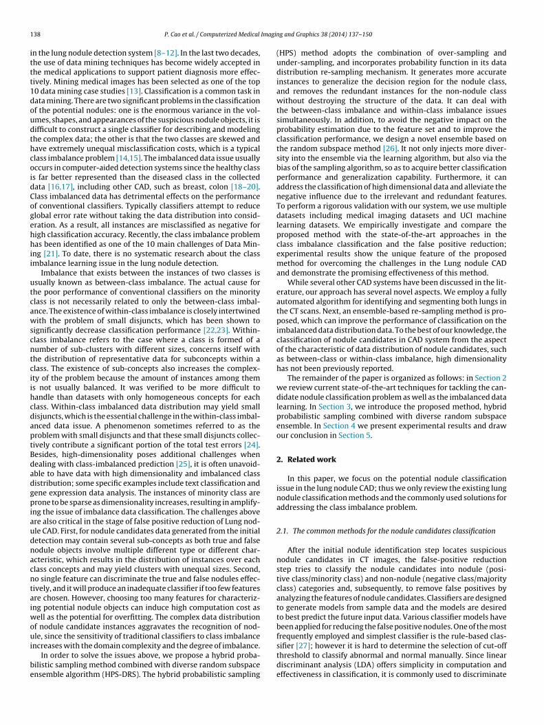

1 Imagin

ittt1doudthcoidCogehhii

utcawscntciihcdaptBdadgpiaudnacntaiwoui

be

38 P. Cao et al. / Computerized Medical

n the lung nodule detection system [8–12]. In the last two decades,he use of data mining techniques has become widely accepted inhe medical applications to support patient diagnosis more effec-ively. Mining medical images has been selected as one of the top0 data mining case studies [13]. Classification is a common task inata mining. There are two significant problems in the classificationf the potential nodules: one is the enormous variance in the vol-mes, shapes, and appearances of the suspicious nodule objects, it isifficult to construct a single classifier for describing and modelinghe complex data; the other is that the two classes are skewed andave extremely unequal misclassification costs, which is a typicallass imbalance problem [14,15]. The imbalanced data issue usuallyccurs in computer-aided detection systems since the healthy classs far better represented than the diseased class in the collectedata [16,17], including other CAD, such as breast, colon [18–20].lass imbalanced data has detrimental effects on the performancef conventional classifiers. Typically classifiers attempt to reducelobal error rate without taking the data distribution into consid-ration. As a result, all instances are misclassified as negative forigh classification accuracy. Recently, the class imbalance problemas been identified as one of the 10 main challenges of Data Min-

ng [21]. To date, there is no systematic research about the classmbalance learning issue in the lung nodule detection.

Imbalance that exists between the instances of two classes issually known as between-class imbalance. The actual cause forhe poor performance of conventional classifiers on the minoritylass is not necessarily related to only the between-class imbal-nce. The existence of within-class imbalance is closely intertwinedith the problem of small disjuncts, which has been shown to

ignificantly decrease classification performance [22,23]. Within-lass imbalance refers to the case where a class is formed of aumber of sub-clusters with different sizes, concerns itself withhe distribution of representative data for subconcepts within alass. The existence of sub-concepts also increases the complex-ty of the problem because the amount of instances among thems not usually balanced. It was verified to be more difficult toandle than datasets with only homogeneous concepts for eachlass. Within-class imbalanced data distribution may yield smallisjuncts, which is the essential challenge in the within-class imbal-nced data issue. A phenomenon sometimes referred to as theroblem with small disjuncts and that these small disjuncts collec-ively contribute a significant portion of the total test errors [24].esides, high-dimensionality poses additional challenges whenealing with class-imbalanced prediction [25], it is often unavoid-ble to have data with high dimensionality and imbalanced classistribution; some specific examples include text classification andene expression data analysis. The instances of minority class arerone to be sparse as dimensionality increases, resulting in amplify-

ng the issue of imbalance data classification. The challenges abovere also critical in the stage of false positive reduction of Lung nod-le CAD. First, for nodule candidates data generated from the initialetection may contain several sub-concepts as both true and falseodule objects involve multiple different type or different char-cteristic, which results in the distribution of instances over eachlass concepts and may yield clusters with unequal sizes. Second,o single feature can discriminate the true and false nodules effec-ively, and it will produce an inadequate classifier if too few featuresre chosen. However, choosing too many features for characteriz-ng potential nodule objects can induce high computation cost as

ell as the potential for overfitting. The complex data distributionf nodule candidate instances aggravates the recognition of nod-le, since the sensitivity of traditional classifiers to class imbalance

ncreases with the domain complexity and the degree of imbalance.In order to solve the issues above, we propose a hybrid proba-

ilistic sampling method combined with diverse random subspacensemble algorithm (HPS-DRS). The hybrid probabilistic sampling

g and Graphics 38 (2014) 137– 150

(HPS) method adopts the combination of over-sampling andunder-sampling, and incorporates probability function in its datadistribution re-sampling mechanism. It generates more accurateinstances to generalize the decision region for the nodule class,and removes the redundant instances for the non-nodule classwithout destroying the structure of the data. It can deal withthe between-class imbalance and within-class imbalance issuessimultaneously. In addition, to avoid the negative impact on theprobability estimation due to the feature set and to improve theclassification performance, we design a novel ensemble based onthe random subspace method [26]. It not only injects more diver-sity into the ensemble via the learning algorithm, but also via thebias of the sampling algorithm, so as to acquire better classificationperformance and generalization capability. Furthermore, it canaddress the classification of high dimensional data and alleviate thenegative influence due to the irrelevant and redundant features.To perform a rigorous validation with our system, we use multipledatasets including medical imaging datasets and UCI machinelearning datasets. We empirically investigate and compare theproposed method with the state-of-the-art approaches in theclass imbalance classification and the false positive reduction;experimental results show the unique feature of the proposedmethod for overcoming the challenges in the Lung nodule CADand demonstrate the promising effectiveness of this method.

While several other CAD systems have been discussed in the lit-erature, our approach has several novel aspects. We employ a fullyautomated algorithm for identifying and segmenting both lungs inthe CT scans. Next, an ensemble-based re-sampling method is pro-posed, which can improve the performance of classification on theimbalanced data distribution data. To the best of our knowledge, theclassification of nodule candidates in CAD system from the aspectof the characteristic of data distribution of nodule candidates, suchas between-class or within-class imbalance, high dimensionalityhas not been previously reported.

The remainder of the paper is organized as follows: in Section 2we review current state-of-the-art techniques for tackling the can-didate nodule classification problem as well as the imbalanced datalearning. In Section 3, we introduce the proposed method, hybridprobabilistic sampling combined with diverse random subspaceensemble. In Section 4 we present experimental results and drawour conclusion in Section 5.

2. Related work

In this paper, we focus on the potential nodule classificationissue in the lung nodule CAD; thus we only review the existing lungnodule classification methods and the commonly used solutions foraddressing the class imbalance problem.

2.1. The common methods for the nodule candidates classification

After the initial nodule identification step locates suspiciousnodule candidates in CT images, the false-positive reductionstep tries to classify the nodule candidates into nodule (posi-tive class/minority class) and non-nodule (negative class/majorityclass) categories and, subsequently, to remove false positives byanalyzing the features of nodule candidates. Classifiers are designedto generate models from sample data and the models are desiredto best predict the future input data. Various classifier models havebeen applied for reducing the false positive nodules. One of the mostfrequently employed and simplest classifier is the rule-based clas-

sifier [27]; however it is hard to determine the selection of cut-offthreshold to classify abnormal and normal manually. Since lineardiscriminant analysis (LDA) offers simplicity in computation andeffectiveness in classification, it is commonly used to discriminate

Imagin

tnetcicoSn[tdo

tcdrdalnpdspAw

2

wfllahmapdutdSaioo[icslycd

hacrcm

P. Cao et al. / Computerized Medical

he potential nodule [11,28]. More sophisticated classifiers such aseural network (NN) and support vector machine (SVM) are oftenmployed in nodule recognition tasks [8,10,29–31], which havehe ability to learn complex input–output relationships automati-ally, and have low dependence on domain specific knowledge. Anmportant new trend is the appearance of ensemble learners whichombine the decisions of multiple classifiers to form an integratedutput, so as to enhance the generalization ability of a single model.uzuki et al. have proposed a pixel-based massive training artificialeural network (MTANN) for distinction between nodule and FPs10]. Lee et al. developed a random forest ensemble classificationo improve the nodule classification performance [32]. Dolejsi et al.esigned a Asymmetric Adaboost ensemble to reduce the numberf FPs [33].

There is an important problem in the classification of poten-ial nodule data. The dataset is typically imbalanced, and theosts of misclassification are different. Class imbalanced data hasetrimental effects on the performance of conventional classifiers,esulting in lowering the performance of discrimination in the can-idate nodule. However, in nodule classification, the problem hasttracted less attention. Only a few publications address this prob-em. The authors in [8] use Tomek links to remove borderline falseodule cases in order to achieve 100% sensitivity. Campadelli et al.rove that cost-sensitive SVM (CS-SVM) trained with imbalancedata sets achieves promising results in terms of sensitivity andpecificity, by means of adjusting the misclassification cost of falseositives versus false negatives [31]. Dolejsi et al. use asymmetricdaboost learning to improve the sensitivity by setting differenteights for two classes [33].

.2. The common methods for the class imbalance problem

Not only in the medical lesion detection domain, many real-orld applications, such as spam filtering, text classification and

raud detection in business transactions, have problems whenearning from imbalanced data sets. In recent years, the imbalancedearning problem has drawn a significant amount of interest fromcademia, industry, and government funding agencies. Much workas been done in addressing the class imbalance problem. Theseethods can be grouped in two categories: the data perspective

nd the algorithm perspective [15]. The methods with the dataerspective re-balance the class distribution by re-sampling theata space, either over-sampling instances of the minority class ornder-sampling instances of the majority class. The re-samplingechniques try to balance out the dataset either randomly oreterministically. A widely used over-sampling technique is calledMOTE (Synthetic Minority Over-sampling Technique), which cre-tes synthetic samples between each positive sample and one ofts neighbors [34]. SMOTE is effective to increase the significancef the positive class in the decision region. There exist many meth-ds based on the SMOTE for generating more appropriate instances35,36]. The methods with the algorithm perspective adapt exist-ng common classifier learning algorithms to bias toward the smalllass, such as one-class learning and cost sensitive learning. Cost-ensitive learning is one of the most important topics in machineearning and data mining, and has attracted high attention in recentears. It takes misclassification costs into account during the modelonstruction, and does not modify the imbalanced data distributionirectly [37–39].

As we have stated, in recent years, ensemble of classifiersave arisen as a possible solution to the class imbalance problemttracting great interest among researcher because of their flexible

haracteristics [40]. Ensembles are designed to increase the accu-acy of a single classifier by training several different classifiers andombining their decisions to output a single class label. Not onlyultiple classifiers could have better answer than a single one, but

g and Graphics 38 (2014) 137– 150 139

also the ensemble framework provides diversity for avoiding theoverfitting of some algorithms. Bagging and Boosting are two ofthe most popular techniques; the Easyensemble method is devel-oped based on the Bagging classification [41]. SMOTEBoost [36] isdesigned to alter the imbalanced distribution based on Boosting.Data generation techniques are involved to emphasize the minorityclass examples at each iteration of Boosting. The ensemble com-bined with cost sensitive learning can enhance the performancedue to the diversity of the ensemble, such as AdaCost [42]. andMetaCost [43].

3. HRS-DRS method

In this section, we begin by describing the hybrid probabilisticsampling. We then describe how to incorporate this method intothe diverse random subspace ensemble to create HPS-DRS.

3.1. Hybrid probabilistic sampling

Gaussian mixture models (GMM) are generative probabilisticmodels of several Gaussian distributions for density estimation inmachine learning applications. A Gaussian mixture can be con-structed to acceptably approximate any given density. Therefore,we assume the distribution of two classes follows the Gaussian mix-ture model with unknown parameters. The parametric probabilitydensity function of GMM is defined as a weighted sum of Gauss-ians. The finite Gaussian mixture model with k components may bewritten as:

p(y|�1, . . ., �k; �1, . . ., �k; �1, . . ., �k) =∑k

j=1�jN(�j, �j) (1)

and

0 ≤ �j ≤ 1,∑k

j=1�j = 1 (2)

where �j are the means, �j are covariance matrixes, �j are the mix-ing proportions, and N(�j, �j) is a Gaussian with specified mean andvariance.

We need to estimate the parameters of GMM with the existinginstances of both the classes. The standard method used to fit finitemixture models to observe data is the expectation-maximization(EM) algorithm, which converges to a maximum likelihood esti-mate of the mixture parameters. However, the drawbacks are thatit is sensitive to initialization and it requires the number of compo-nents to be set by users. Since the FJ algorithm [44] tries to overcomethe major weaknesses of the basic EM algorithm particularly vis-à-vis the initialization, and can automatically select the number ofcomponent, we use it here to estimate the parameters of GMM.

Each instance xi will then be assigned to the cluster k where ithas the largest posterior probability p(k|xi). When calculating theprobability of each instance on each component, the probabilitiesfor the numeric attributes is obtained by a Gaussian density func-tion, and for the nominal attributes, the probabilities of occurrenceof each distinct value are determined using Laplace estimates. Atthe same time, we obtain the parameters of each Gaussian com-ponent. For different clusters, the re-sampling rates are different;within the cluster, the probabilities of each instance to be chose forre-sampled are different.

We use the over-sampling combined with under-sampling tobalance the class size. The sizes of the two classes are Mneg and Mpos.The gap G between two uneven classes is: G = Mneg − Mpos. Thus,the amount of instances in the positive class for over-sampling

is: Npos = G × ˛, and the amount of instances in the negative classfor under-sampling is: Nneg = G × (1 − ˛). To adjust the within classimbalance, we need to balance cluster sizes in each class. Forthe positive class, the number of instances to be over-sampled is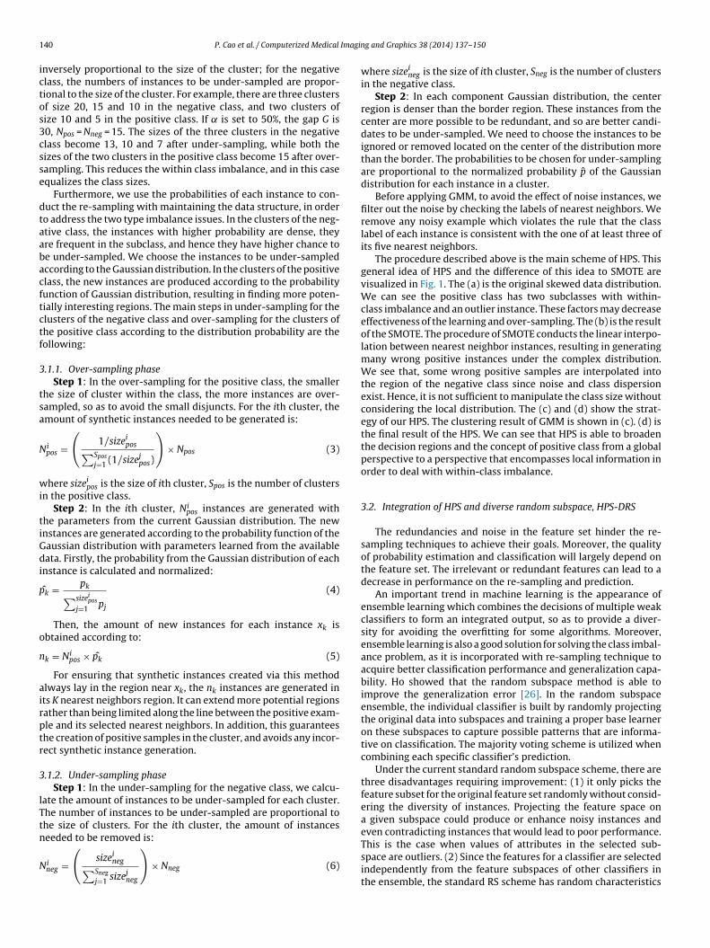

1 Imagin

ictos3csse

dtaabacftctf

3

tsa

N

wi

tiGdi

p

o

n

airptr

3

lTtn

N

40 P. Cao et al. / Computerized Medical

nversely proportional to the size of the cluster; for the negativelass, the numbers of instances to be under-sampled are propor-ional to the size of the cluster. For example, there are three clustersf size 20, 15 and 10 in the negative class, and two clusters ofize 10 and 5 in the positive class. If ̨ is set to 50%, the gap G is0, Npos = Nneg = 15. The sizes of the three clusters in the negativelass become 13, 10 and 7 after under-sampling, while both theizes of the two clusters in the positive class become 15 after over-ampling. This reduces the within class imbalance, and in this casequalizes the class sizes.

Furthermore, we use the probabilities of each instance to con-uct the re-sampling with maintaining the data structure, in ordero address the two type imbalance issues. In the clusters of the neg-tive class, the instances with higher probability are dense, theyre frequent in the subclass, and hence they have higher chance toe under-sampled. We choose the instances to be under-sampledccording to the Gaussian distribution. In the clusters of the positivelass, the new instances are produced according to the probabilityunction of Gaussian distribution, resulting in finding more poten-ially interesting regions. The main steps in under-sampling for thelusters of the negative class and over-sampling for the clusters ofhe positive class according to the distribution probability are theollowing:

.1.1. Over-sampling phaseStep 1: In the over-sampling for the positive class, the smaller

he size of cluster within the class, the more instances are over-ampled, so as to avoid the small disjuncts. For the ith cluster, themount of synthetic instances needed to be generated is:

ipos =

(1/sizei

pos∑Spos

j=1 (1/sizejpos)

)× Npos (3)

here sizeipos is the size of ith cluster, Spos is the number of clusters

n the positive class.Step 2: In the ith cluster, Ni

pos instances are generated withhe parameters from the current Gaussian distribution. The newnstances are generated according to the probability function of theaussian distribution with parameters learned from the availableata. Firstly, the probability from the Gaussian distribution of each

nstance is calculated and normalized:

k̂ = pk∑sizeipos

j=1 pj

(4)

Then, the amount of new instances for each instance xk isbtained according to:

k = Nipos × p̂k (5)

For ensuring that synthetic instances created via this methodlways lay in the region near xk, the nk instances are generated ints K nearest neighbors region. It can extend more potential regionsather than being limited along the line between the positive exam-le and its selected nearest neighbors. In addition, this guaranteeshe creation of positive samples in the cluster, and avoids any incor-ect synthetic instance generation.

.1.2. Under-sampling phaseStep 1: In the under-sampling for the negative class, we calcu-

ate the amount of instances to be under-sampled for each cluster.he number of instances to be under-sampled are proportional tohe size of clusters. For the ith cluster, the amount of instances

eeded to be removed is:

ineg =

(sizei

neg∑Sneg

j=1 sizejneg

)× Nneg (6)

g and Graphics 38 (2014) 137– 150

where sizeineg is the size of ith cluster, Sneg is the number of clusters

in the negative class.Step 2: In each component Gaussian distribution, the center

region is denser than the border region. These instances from thecenter are more possible to be redundant, and so are better candi-dates to be under-sampled. We need to choose the instances to beignored or removed located on the center of the distribution morethan the border. The probabilities to be chosen for under-samplingare proportional to the normalized probability p̂ of the Gaussiandistribution for each instance in a cluster.

Before applying GMM, to avoid the effect of noise instances, wefilter out the noise by checking the labels of nearest neighbors. Weremove any noisy example which violates the rule that the classlabel of each instance is consistent with the one of at least three ofits five nearest neighbors.

The procedure described above is the main scheme of HPS. Thisgeneral idea of HPS and the difference of this idea to SMOTE arevisualized in Fig. 1. The (a) is the original skewed data distribution.We can see the positive class has two subclasses with within-class imbalance and an outlier instance. These factors may decreaseeffectiveness of the learning and over-sampling. The (b) is the resultof the SMOTE. The procedure of SMOTE conducts the linear interpo-lation between nearest neighbor instances, resulting in generatingmany wrong positive instances under the complex distribution.We see that, some wrong positive samples are interpolated intothe region of the negative class since noise and class dispersionexist. Hence, it is not sufficient to manipulate the class size withoutconsidering the local distribution. The (c) and (d) show the strat-egy of our HPS. The clustering result of GMM is shown in (c). (d) isthe final result of the HPS. We can see that HPS is able to broadenthe decision regions and the concept of positive class from a globalperspective to a perspective that encompasses local information inorder to deal with within-class imbalance.

3.2. Integration of HPS and diverse random subspace, HPS-DRS

The redundancies and noise in the feature set hinder the re-sampling techniques to achieve their goals. Moreover, the qualityof probability estimation and classification will largely depend onthe feature set. The irrelevant or redundant features can lead to adecrease in performance on the re-sampling and prediction.

An important trend in machine learning is the appearance ofensemble learning which combines the decisions of multiple weakclassifiers to form an integrated output, so as to provide a diver-sity for avoiding the overfitting for some algorithms. Moreover,ensemble learning is also a good solution for solving the class imbal-ance problem, as it is incorporated with re-sampling technique toacquire better classification performance and generalization capa-bility. Ho showed that the random subspace method is able toimprove the generalization error [26]. In the random subspaceensemble, the individual classifier is built by randomly projectingthe original data into subspaces and training a proper base learneron these subspaces to capture possible patterns that are informa-tive on classification. The majority voting scheme is utilized whencombining each specific classifier’s prediction.

Under the current standard random subspace scheme, there arethree disadvantages requiring improvement: (1) it only picks thefeature subset for the original feature set randomly without consid-ering the diversity of instances. Projecting the feature space ona given subspace could produce or enhance noisy instances andeven contradicting instances that would lead to poor performance.

This is the case when values of attributes in the selected sub-space are outliers. (2) Since the features for a classifier are selectedindependently from the feature subspaces of other classifiers inthe ensemble, the standard RS scheme has random characteristics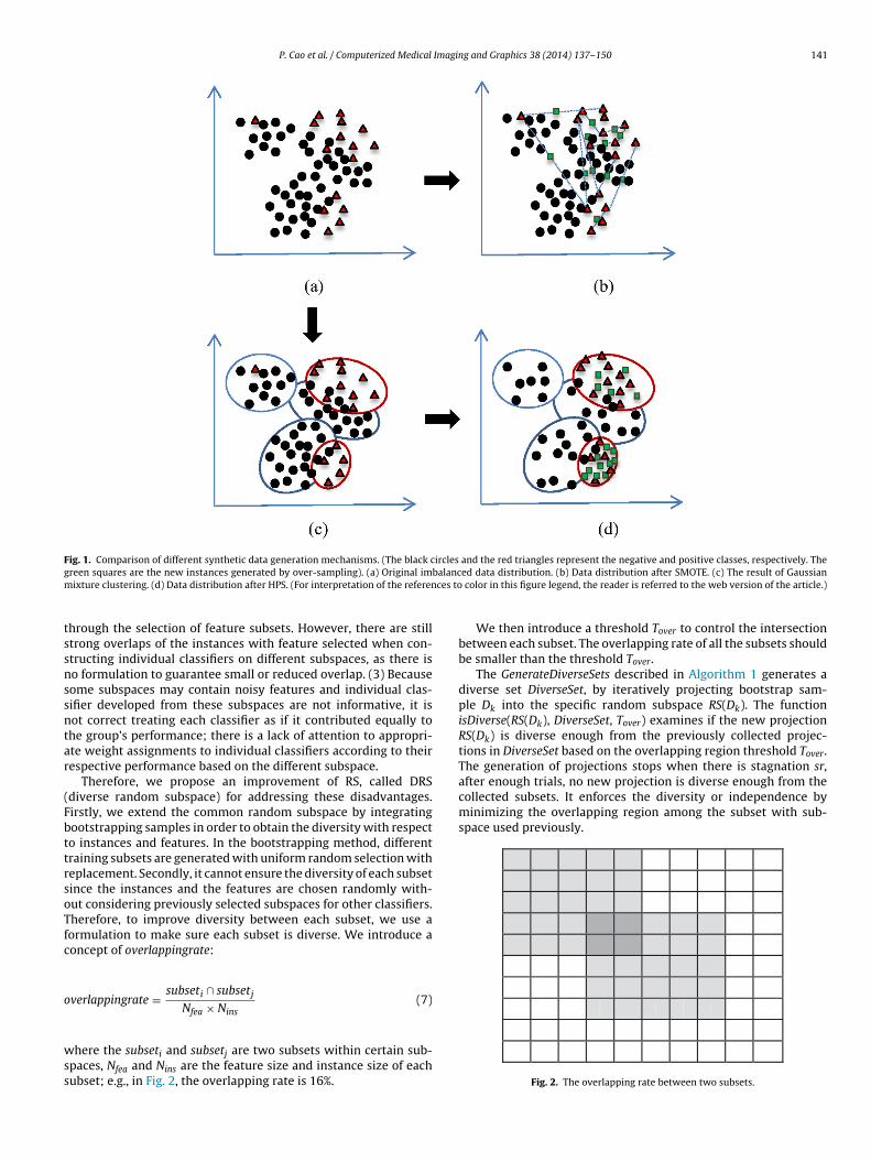

P. Cao et al. / Computerized Medical Imaging and Graphics 38 (2014) 137– 150 141

Fig. 1. Comparison of different synthetic data generation mechanisms. (The black circles and the red triangles represent the negative and positive classes, respectively. Theg balancm ces to

tssnssntar

(FbttrsoTfc

o

wss

collected subsets. It enforces the diversity or independence byminimizing the overlapping region among the subset with sub-space used previously.

reen squares are the new instances generated by over-sampling). (a) Original imixture clustering. (d) Data distribution after HPS. (For interpretation of the referen

hrough the selection of feature subsets. However, there are stilltrong overlaps of the instances with feature selected when con-tructing individual classifiers on different subspaces, as there iso formulation to guarantee small or reduced overlap. (3) Becauseome subspaces may contain noisy features and individual clas-ifier developed from these subspaces are not informative, it isot correct treating each classifier as if it contributed equally tohe group’s performance; there is a lack of attention to appropri-te weight assignments to individual classifiers according to theirespective performance based on the different subspace.

Therefore, we propose an improvement of RS, called DRSdiverse random subspace) for addressing these disadvantages.irstly, we extend the common random subspace by integratingootstrapping samples in order to obtain the diversity with respecto instances and features. In the bootstrapping method, differentraining subsets are generated with uniform random selection witheplacement. Secondly, it cannot ensure the diversity of each subsetince the instances and the features are chosen randomly with-ut considering previously selected subspaces for other classifiers.herefore, to improve diversity between each subset, we use aormulation to make sure each subset is diverse. We introduce aoncept of overlappingrate:

verlappingrate = subseti ∩ subsetj

Nfea × Nins(7)

here the subseti and subsetj are two subsets within certain sub-paces, Nfea and Nins are the feature size and instance size of eachubset; e.g., in Fig. 2, the overlapping rate is 16%.

ed data distribution. (b) Data distribution after SMOTE. (c) The result of Gaussian color in this figure legend, the reader is referred to the web version of the article.)

We then introduce a threshold Tover to control the intersectionbetween each subset. The overlapping rate of all the subsets shouldbe smaller than the threshold Tover.

The GenerateDiverseSets described in Algorithm 1 generates adiverse set DiverseSet, by iteratively projecting bootstrap sam-ple Dk into the specific random subspace RS(Dk). The functionisDiverse(RS(Dk), DiverseSet, Tover) examines if the new projectionRS(Dk) is diverse enough from the previously collected projec-tions in DiverseSet based on the overlapping region threshold Tover.The generation of projections stops when there is stagnation sr,after enough trials, no new projection is diverse enough from the

Fig. 2. The overlapping rate between two subsets.

1 Imaging and Graphics 38 (2014) 137– 150

AR

E

1234567891

sdpptvbwitmiGob

G

s

wbT

AR

1234

567891

11

sarc

42 P. Cao et al. / Computerized Medical

lgorithm 1. [GenerateDiverseSets]equire:

Training dataset, Dtrain

Ratio of bootstrap samples, Rs

Ratio of feature subspace, Rf

Overlapping region threshold, Tover

Stagnation rate, sr = 100nsure:

Diverse dataSets, DiverseSets: change = 0 ; DiverseSet = {}: while change < sr do: A bootstrap sample Dk selected with replacement from Dtrain with Rs

: Select an random subspace with Rf from Dk

: if isDiverse(subspace(Dk), DiverseSet, Tover) = = true then: DiverseSet . add(subspace(Dk)) ; change = 0 ;: else: change = change+ 1 ;: end if0: end while

Thirdly, we employ a weighted average while combining clas-ifiers according to the performance of each component. In theiverse subsets, some of the selected subspaces may have bettererformance on the imbalanced dataset; others lack the ability toroperly discriminate between the different classes. We utilizedhe out-of-bag (OOB) samples in determining different classifier’soting power, and then each base classifier is weighted when com-ined to create the final decision function. The goal is to assigneights that reflect the relative contribution of each classifier in

mproving the overall performance of the ensemble. It is knownhat the use of overall accuracy is not an appropriate evaluation

easure for imbalanced data, therefore the metric for represent-ng the performance of each classifier is chosen by G-mean. The-mean is the geometric mean of accuracies measured separatelyn each class, which is commonly utilized when performance ofoth classes is concerned and expected to be high simultaneously.

-mean =√

sensitivity × specificity (8)

ensitivity = TPTP + FN

, specificity = TNTN + FP

(9)

here TP denotes the number of true positives, FP denotes the num-er of false positives, FN denotes the number of false negatives, andN the number of true negatives.

The HPS-DRS algorithm is described in Algorithm 2.

lgorithm 2. [HPS-DRS]equire:

Training Dataset Dtrain , Test Dataset Dtest , Ratio of bootstrap samplesRs , Ratio of feature subspace Rf , Overlapping region threshold Tover ,Hybrid sampling ratio parameter ˛

Training:: Ensemble = NULL: DiverseSets=GenerateDiverseSets(Dtrain ,Rs ,Rf ,Tover): for each subset Dk in DiverseSets do: Apply HPS on the subset Dk , and generate a new balanced set BDk

s

with ˛: Construct a classifier Ck on the BDk

: Evaluate Ck on the OOB(Dk) and obtain the value of G-mean, GMk

: Ck . Subspace = Subspace(Dk); Ck . GM = GMk

: end for: Ensemble = Ensemble ∪ Ck

0: Calculate and normalize the weights of each classifier in Ensembleaccording to its GM

Testing:1: Calculate output from each classifier of Ensemble with Dtest

2: Generate the final output by aggregating all the outputs withweighted voting

To reduce the learning time of HPS-DRS, the procedure of

ampling and learning in each subset Dk can be carried out in par-llel before aggregating. Moreover, each classifier is trained in theeduced subset with fewer instances and features. Therefore theomputational time is acceptable.

Fig. 3. The scheme of the nodule detection.

Since data often exhibits characteristics at a local rather thanglobal level, DRS can find more valuable local data properties so asto improve the quality of sampling. Moreover, the different imbal-anced data distribution in each random subset makes the ensembleclassifier robust to the evolving testing distribution. Furthermore,DRS can alleviate the effect of class overlapping on the imbalanceddata distribution [45], since the two classes may be separable insome reduced subspace.

4. Experimental study

4.1. CAD system

Unlike other publications in which candidate nodules wereselected manually for classification evaluation, we obtained theappropriate candidate nodule samples objectively using a candi-date nodule detection algorithm. Our CAD scheme also containslung segmentation, candidate nodule detection and VOI segmenta-tion. The sequence of steps for our scheme is shown in Fig. 3.

4.2. Initial nodule detection

Our database consists of 165 thin section CT scans with 192 solidnodules, obtained from the Guangzhou hospital and the Shenyanghospital in China. These databases included nodules of differentsizes (3–30 mm). The nodule locations of these scans are markedconsensually by three experienced expert radiologists.

In the detection phase, we use the dot enhancement filter pro-posed by Li [46], which is aimed to simultaneously enhance objectsof a specific structure (e.g. dot-like nodules) and suppress objects ofother structures (e.g. line-like vessels) in multi-scale. If the nodulediameters are in the range [dmin, dmax], the scales to be consideredfor the Gaussian smoothing will be in the range [dmin/4, dmax/4]. Theamount of scales is set to 5. After the 3D selective enhancement Hes-sian filter is applied on the original image, we use a thresholdingtechnique and a 3D connected-component labeling technique toseparate nodule candidates and identify all of the isolated objects[47]. The value of the threshold in the thresholding technique is setto 40, and objects with an effective diameter smaller than 2.5 mmwere considered to be non-nodules and were eliminated [47].

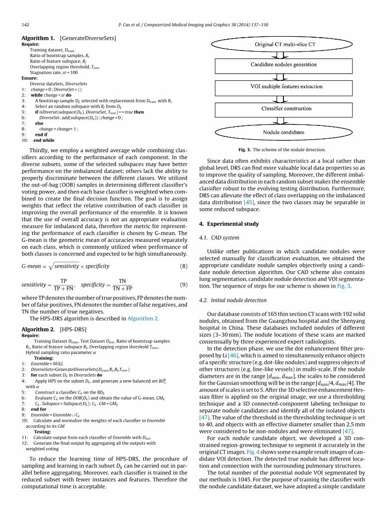
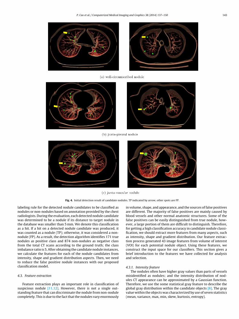
For each nodule candidate object, we developed a 3D con-strained region-growing technique to segment it accurately in theoriginal CT images. Fig. 4 shows some example result images of can-didate VOI detection. The detected true nodule has different loca-

tion and connection with the surrounding pulmonary structures.

The total number of the potential nodule VOI segmentated byour methods is 1045. For the purpose of training the classifier withthe nodule candidate dataset, we have adopted a simple candidate

P. Cao et al. / Computerized Medical Imaging and Graphics 38 (2014) 137– 150 143

odule

lnrwtawnnfiwitc

4

ssc

Fig. 4. Initial detection result of candidate n

abeling rule for the detected nodule candidates to be classified asodules or non-nodules based on annotation provided by the chestadiologists. During the evaluation, each detected nodule candidateas determined to be a nodule if its distance to target nodule in

he database was smaller than 5 mm. We denote this classifications a hit. If a hit on a detected nodule candidate was produced, itas counted as a nodule (TP); otherwise, it was considered a non-odule (FP). As a result, the detection algorithm identifies 171 trueodules as positive class and 874 non-nodules as negative class

rom the total CT scans according to the ground truth; the classmbalance ratio is 5. After obtaining the candidate nodule instances,

e calculate the features for each of the nodule candidates fromntensity, shape and gradient distribution aspects. Then, we needo reduce the false positive nodule instances with our proposedlassification model.

.3. Feature extraction

Feature extraction plays an important role in classification ofuspicious nodule [11,12]. However, there is not a single out-tanding feature that can discriminate the nodule from non-noduleompletely. This is due to the fact that the nodules vary enormously

s. TP indicated by arrow, other spots are FP.

in volume, shape, and appearance, and the sources of false positivesare different. The majority of false positives are mainly caused byblood vessels and other normal anatomic structures. Some of thefalse positives can be easily distinguished from true nodule, how-ever, a large portion of them are difficult to distinguish. Therefore,for getting a high classification accuracy in candidate nodule classi-fication, we should extract more features from many aspects, suchas intensity, shape and gradient distribution. Our feature extrac-tion process generated 43 image features from volume of interest(VOI) for each potential nodule object. Using these features, weconstruct the input space for our classifiers. This section gives abrief introduction to the features we have collected for analysisand selection.

4.3.1. Intensity featureThe nodules often have higher gray values than parts of vessels

misidentified as nodules; and the intensity distribution of nod-ules CT appearance can be approximated by a Gaussian function.

Therefore, we use the some statistical gray feature to describe theglobal gray distribution within the candidate objects [8]. The grayvalue within the objects was characterized by use of seven statistics(mean, variance, max, min, skew, kurtosis, entropy).

1 Imagin

awTsI

R

wp√t

4

tsatw[

siad

S

C

a(ei1

4

fotoaa

G

e

wog

dctd

44 P. Cao et al. / Computerized Medical

Meanwhile, for capturing the volume intensity distributionlong the radial direction of the three dimension nodule candidates,e extract the feature of radial intensity distribution (RIS) [48].

he vector of radial intensity distribution feature for nodule objecthould be decreasing, while for non-nodule it changes irregularly.t is computed as follows:

IS(ri+1, ri) =∑

iI(xi, yi, zi) (10)

here I(xi, yi, zi) denotes the intensity value in theosition of (xi, yi, zi), and (xi, yi, zi) ∈ {(xi, yi, zi)|ri <

(xi − xc)2 + (yi − yc)2 + (zi − zc)2}, (xc, yc, zc) is the coordinate ofhe center.

.3.2. Shape featureBased on the fact that an isolated nodule or a nodule attached

o a blood vessel is generally either depicted as a sphere or hasome spherical elements, while a blood vessel is usually oblong. Wettempt to distinguish true nodules from false ones by calculatinghe volumetric shape index (SI) and curvedness (CV) [49–51], asell as other explicit shape features to characterize the 3D shape

47].Shape index is a measure of the shape, which represents the local

hape feature at each voxel while being less sensitive to the imagentensity. Every distinct shape, except for the plane, corresponds to

unique SI. The volumetric shape index (SI) at each voxel p can beefined as:

I(p) = 12

− 1�

arctank1(p) + k2(p)k1(p) − k2(p)

√k2

1 + k22

2(11)

V(p) =√

k21(p) + k2

2(p)2

(12)

The SI and CV features are calculated based on every pixel,nd they are further characterized by seven statistical operationsmean, variance, max, min, skew, kurtosis, entropy). Some otherxplicit shape features were also extracted from candidate object,ncluding the volume, the surface area and compactness. Features3–29 describe the intensity distribution from the VOI in Table 1.

.3.3. Gradient distribution featureThe true nodules have a high concentration because they grow

rom the center to surround, thus nodules have high concentrationf gradient vector. We utilize the concentration feature to charac-erize the degree of convergence at voxel p based on the conceptf gradient concentration (GC) [49,52]. In short, the GC feature at

point p characterizes the overall direction of the gradient vectorsround. It is defined by:

C(p) = 1D

∑D

i=1emax

i (p) (13)

maxi (p) = max

Rmin≤n≤Rmax

{1

n + 1

∑N

l=1cos �il(p)

}(14)

here D is the number of the symmetrically direction vectors dl

riginating from p. The angle is calculated between dl and gli, where

li

is the gradient vector located at distance l from p in direction

l. We also calculate the gradient field strength at each pixel. Theoncentration and strength features based on every pixel are fur-her characterized by seven statistical operations. Features 30–43escribe the gradient distribution from the VOI in Table 1.

g and Graphics 38 (2014) 137– 150

4.4. Evaluating the effectiveness of HPS-DRS

We made a vertical comparison and a horizontal comparisonseparately. In the vertical comparison, we tested the HPS-DRS bycomparing our hybrid approach to each individual technique aswell as original RS and Bagging with and without the re-sampling.In the horizontal comparison, we compared the HPS-DRS with thestate-of-the-art methods in the classification of imbalanced data aswell as the current methods for false positive reduction.

In this experiment, we evaluate the effectiveness of our pro-posed HPS-DRS algorithm. Since the DRS framework utilizes theidea of RSM and Bagging, we conduct the comparison between DRS,original random subspace, Bagging as well as the single methodswith or without HPS. We chose neural network (NN) as our baseclassifier. In the setting of the neural network classifier, the num-ber of input neurons is equal to the number of features in the givensubspace, and the number of neurons in the hidden layer is set tobe 10. The sigmoid function is used as the activation function, andthe inner training epochs is set to be 200 with a learning rate of 0.1.

We use metrics such as sensitivity, specificity and G-mean toevaluate the performance of the learning algorithm on imbalancednodule candidate data. To make our comparisons more convincing,we further use the AUC (area under the ROC curve) as the perfor-mance evaluation [30,53] which is a commonly used measurementin medical CAD systems. The AUC measures the performance ofranking a randomly chosen positive example higher than a ran-domly chosen negative example. In this case, it represents theperformance of ranking an instance from the positive class higherthan instances in the negative class. The results show that threeensemble approaches increase performance of the single model byusing multiple different and complementary representations. Wealso use AUC as the measure metric of the weighted voting in theaggregation of DRS ensemble. The ensemble size of all the ensem-ble methods is set to 50. In the parameters setting of HPS, the ̨ isset to 70% for avoiding loss of reducing too many instances, and theparameters K set to 5. In the parameters setting of DRS, Rs is 0.7,Rf is 0.5. The best value of Tover can be obtained from the trainingdata, then the ensemble size can be determined adaptively. In thisexperiment, it is set to 0.4 empirically. It is a good trade-off valuebetween the diversity and the sufficient ensemble size according toexperiments. Although it is not necessarily the best, it can guaran-tee the diversity among each subset. All the experiments are carriedout by means of a 10-fold cross-validation. That is, the dataset wassplit into 10-fold, each one containing 10% of the patterns of thedataset. For each fold, the algorithm is trained with the examplescontained in the remaining folds and then tested with the currentfold. The results are shown in Table 2.

From Table 2, we can observe that the performance of neuralnetwork (NN) is affected by the presence of class imbalance. It isalso apparent that the proposed HPS can improve the performanceof the original NN on the imbalanced nodule candidate data regard-less of the single model or ensemble, which can show that HPS hasthe ability of reducing the bias inherent in the learning proceduredue to the class imbalance. However, the classification performancebased on only HPS did not achieve the best, since the over-samplingperformed on the whole space cannot get the optimal re-samplingquality due to the fact that redundant or irrelevant features exist.

The experimental results also demonstrated that the DiverseRandom Subspace (DRS) ensemble framework, especially designedfor imbalanced problems, obtained a more generalized perfor-mance for high-dimensional and imbalanced potential nodule data.The mechanism of aggregating each component with weighted

voting power using G-mean is beneficial for the imbalanced data,because it treat each classifier unequally and assign the appropriateweight to each classifier based on each performance on the imbal-anced data. Moreover, the distribution of the class overlapping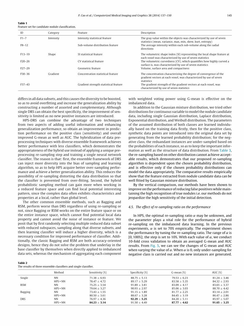

P. Cao et al. / Computerized Medical Imaging and Graphics 38 (2014) 137– 150 145

Table 1Feature set for candidate nodule classification.

ID Category Feature Description

F1–7 Intensity Intensity statistical feature The gray value within the objects was characterized by use of sevenstatistics (mean, variance, max, min, skew, kurt, entropy)

F8–12 Sub-volume distribution feature The average intensity within each sub-volume along the radialdirections

F13–19 Shape SI statistical feature The volumetric shape index (SI) representing the local shape feature ateach voxel was characterized by use of seven statistics

F20–26 CV statistical feature The volumetric curvedness (CV), which quantifies how highly curved asurface is, was characterized by use of seven statistics

F27–29 Geometric feature Volume, surface area and compactness

F30–36 Gradient Concentration statistical feature The concentration characterizing the degree of convergence of thegradient vectors at each voxel, was characterized by use of seven

dscss

fgtipbapccamptpapp

Rntppwtntdbd

TT

F37–43 Gradient strength statistical feature

iffers in all data subsets, and this causes the diversity to be boosted,o as to avoid overfitting and increase the generalization ability byonstructing a number of assorted and complementary. Althoughingle DRS can obtain the best specificity, the improvement of sen-itivity is limited as no new positive instances are introduced.

HPS-DRS can combine the advantage of two techniquesrom two aspects of adding useful information and enhancingeneralization performance, so obtain an improvement in predic-ion performance on the positive class (sensitivity) and overallmproved G-mean as well as AUC. The hybridization of data pre-rocessing techniques with diverse ensemble framework achievesetter performance with less classifiers, which demonstrates theppropriateness of the hybrid use instead of applying a unique pre-rocessing re-sampling step and training a single neural networklassifier. The reason is that: first, the ensemble framework of DRSan inject more diversity into the bias of sampling and learninglgorithm, so as to help HPS acquire better over-sampling perfor-ance and achieve a better generalization ability. This reduces the

ossibility of re-sampling distorting the data distribution so thathe classifier is prevented from over-fitting. Second, the hybridrobabilistic sampling method can gain more when working in

reduced feature space and can find local potential interestingattern, since the complex data often exhibits characteristics androperties at a local, rather than global level.

The other common ensemble methods, such as Bagging andSM, perform worse than DRS regardless of using re-sampling orot, since Bagging or RSM works on the entire feature space or onhe entire instance space, which cannot find potential local dataroperty and cannot avoid the noise of instance or feature. Weosit that by first randomly selecting multiple reduced data subsetith reduced subspaces, sampling along that diverse subsets, and

hen learning classifier will induce a higher diversity, which is aecessary condition for improved performance of classifier. Addi-

ionally, the classic Bagging and RSM are both accuracy-orientedesigns, hence they do not solve the problem that underlay in thease classifier by themselves when directly applied to imbalancedata sets, whereas the mechanism of aggregating each component

able 2he results of three ensemble classifiers and single classifier.

Method Sensitivity (%)

Single NN 71.38 ± 6.93

HPS + NN 78.47 ± 4.72

RSM NN 75.25 ± 3.54

HPS + NN 79.64 ± 3.27

Bagging NN 73.43 ± 1.55

HPS + NN 80.50 ± 3.61

DRS NN 76.97 ± 4.36

HPS + NN 84.23 ± 3.14

statisticsThe gradient strength of the gradient vectors at each voxel, wascharacterized by use of seven statistics

with weighted voting power using G-mean is effective on theimbalanced data.

In addition to the Gaussian mixture distribution, we tried otherdistributions for continuous variable to model the nodule candidatedata, including single Gaussian distribution, Laplace distribution,Exponential distribution, and Weibull distribution. The parametersof the assumed distribution of both classes are learned individu-ally based on the training data firstly, then for the positive class,synthetic data points are introduced into the original data set bygenerating from the learned probability distribution; for the neg-ative class, the reduandant instances are under-sampled based onthe probabilities of each instance, so as to keep the important infor-mation as well as the structure of data distribution. From Table 3,the re-sampling based on other distribution cannot achieve accept-able results, which demonstrates that our proposed re-samplingalgorithm is dependent upon the chosen probability distribution,and is effective only if the chosen probability distributions canmodel the data appropriately. The comparative results empiricallyshow that the feature extracted from nodule candidate data can bewell fitted by Gaussian mixture distribution.

By the vertical comparison, our methods have been shown toimprove on the performance of reducing false positives while main-taining the high recognition of true nodules i.e. our methods do notjeopardize the high sensitivity of the initial detection.

4.5. The effect of re-sampling ratio on the performance

In HPS, the optimal re-sampling ratio ̨ may be unknown, andthe parameter plays a vital role for the performance of hybridre-sampling on the imbalanced data learning. In the previousexperiments, ̨ is set to 70% empirically. The experiment showsthe performance by tuning the re-sampling ratio. The range of ̨ is[0, 100%]; the step is set to 10%. With each value of ˛, we conduct

10-fold cross validation to obtain an averaged G-mean and AUCresults. From Fig. 5, we can see the changes of G-mean and AUCwhen varying the value of ˛. When ̨ is 0, only under-sampling fornegative class is carried out and no new instances are generated.

Specificity (%) G-mean (%) AUC (%)

88.75 ± 5.13 79.53 ± 6.23 81.24 ± 3.4689.17 ± 5.29 83.58 ± 5.35 84.32 ± 2.9391.89 ± 3.81 83.09 ± 4.17 83.65 ± 3.3790.93 ± 2.97 85.06 ± 3.03 88.70 ± 4.4291.15 ± 1.89 81.77 ± 2.25 83.14 ± 2.0188.67 ± 3.28 84.45 ± 3.19 86.47 ± 2.8692.29 ± 5.25 84.20 ± 5.11 85.97 ± 5.0791.50 ± 4.49 87.77 ± 4.62 91.65 ± 3.25

146 P. Cao et al. / Computerized Medical Imaging and Graphics 38 (2014) 137– 150

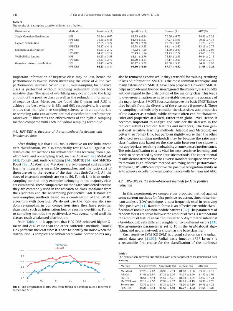
Table 3The results of re-sampling based on different distribution.

Distribution Method Sensitivity (%) Specificity (%) G-mean (%) AUC (%)

Single Gaussian distribution HPS 70.84 ± 6.65 82.75 ± 6.24 76.56 ± 6.77 79.92 ± 5.32HPS-DRS 71.55 ± 6.48 83.44 ± 5.57 77.27 ± 5.95 79.33 ± 4.74

Laplace distribution HPS 72.65 ± 3.22 85.89 ± 2.70 78.99 ± 3.09 81.23 ± 2.76HPS-DRS 76.37 ± 4.11 86.78 ± 3.35 81.41 ± 3.62 83.19 ± 2.77

Exponential distribution HPS 66.23 ± 2.17 77.62 ± 1.59 71.70 ± 2.09 74.36 ± 2.07HPS-DRS 64.77 ± 2.14 79.43 ± 1.54 71.73 ± 2.22 73.65 ± 1.78

Weibull distribution HPS 69.23 ± 3.58 83.11 ± 2.76 75.85 ± 2.95 80.44 ± 2.16

IppcnaoasrMm

4i

dsr[Bltssattoaddrc

mLd

FG

HPS-DRS 72.37 ± 2.72Gaussian mixture distribution HPS 78.47 ± 4.72

HPS-DRS 84.23 ± 3.14

mportant information of negative class may be lost, hence theerformance is lowest. When increasing the value of ˛, the twoerformances increase. When ̨ is 1, over-sampling for positivelass is performed without removing redundant instances foregative class. The issue of overfitting may occur due to the largemount of the positive class as well as the redundant informationf negative class. Moreover, we found the G-mean and AUC tochieve the best when ̨ is 65% and 60% respectively. It demon-trates that the hybrid re-sampling scheme with an appropriatee-sampling ratio can achieve optimal classification performance.oreover, it illustrates the effectiveness of the hybrid samplingethod compared with each individual sampling technique.

.6. HPS-DRS vs. the state-of-the-art methods for dealing withmbalanced data

After finding out that HPS-DRS is effective on the imbalancedata classification, we also empirically test HPS-DRS against thetate-of-the art methods for imbalanced data learning from algo-ithm level and re-sampling level, such as AdaCost [42], MetaCost43], Tomek Link under-sampling [54], SMOTE [34] and SMOTE-oost [36]. AdaCost and MetaCost are two general cost sensitive

earning integrating ensemble approaches, and the ratio cost ofhem are set to the reverse of the size, thus RatioCost = 5. All theizes of ensemble methods are set to 50. Tomek Link is an under-ampling method; only examples belonging to the majority classre eliminated. These comparative methods are considered becausehey are commonly used in the research on class imbalance fromhe algorithm and the re-sampling perspective. SMOTEBoost arever-sampling methods based on a combination of the SMOTElgorithm with Boosting. We do not use the non-heuristic ran-om re-sampling in our comparison since they have potentialrawbacks such as information loss or causing overfitting. For alle-sampling methods, the positive class was oversampled until thelasses reach a balanced distribution.

From Table 4, it is apparent that HPS-DRS achieved higher G-ean and AUC value than the other contender methods. Tomek

ink performs the least since it is hard to identify the noise when theistribution is complex and imbalanced. Some border points may

ig. 5. The performance of HPS-DRS while tuning re-sampling ratio ̨ in terms of-man and AUC.

82.29 ± 3.13 77.17 ± 2.80 82.61 ± 2.7589.17 ± 5.29 83.58 ± 5.35 84.32 ± 2.9391.50 ± 4.49 87.77 ± 4.62 91.65 ± 3.25

also be removed as noise while they are useful for training, resultingin loss of information. SMOTE is the most common technique, andmany extensions of SMOTE have been proposed. However, SMOTEhelps in broadening the decision region of the minority class blindlywithout regard to the distribution of the majority class. This leadsto over-generalization so as to inevitably decrease the accuracy ofthe majority class. SMOTEBoost can improve the basic SMOTE sincethey benefit from the diversity of the ensemble framework. Thesere-sampling methods only consider the class skew and propertiesof the dataset as a whole, while datasets often exhibit character-istics and properties at a local, rather than global level. Hence, itbecomes important to analyze and consider the datasets in thereduced subsets (reduced features and instances). The two gen-eral cost sensitive learning methods (AdaCost and MetaCost) arebetter than Tomek Link, but perform slightly worse than the otheradvanced re-sampling methods.It may be because the ratio mis-classification cost based on the size ratio between two classes isnot appropriate, resulting in obtaining an unexpected performance.The misclassification cost is vital for cost sensitive learning, andneeds to be searched by some heuristic methods. The experimentalresults demonstrated that the Diverse Random subspace ensembleframework is an effective method achieving better performance.Moreover, HPS-DRS can improve the positive recognition ability soas to achieve excellent overall performance with G-mean and AUC.

4.7. HPS-DRS vs. the state-of-the-art methods for false positivereduction

In this experiment, we compare our proposed method againstsome current methods for false positive reduction. Linear discrimi-nant analysis (LDA) technique is most frequently used in removingfalse positives [11]. Random forest is an effective ensemble classi-fication of nodule and non-nodule patterns [32]. The parameters ofrandom forest are set as follows: the amount of trees is set to 50 andthe amount of feature at each split is set to 5. Asymmetric AdaBoost(AsyAdaboost) sets different weights for two different errors [33].The asymmetry parameter is set to 10 in the AsyAdaboost algo-

rithm, and neural network is chosen as the base classifier.

Cost sensitive SVM (CS-SVM) is a good solution on the unbal-anced data sets [31,55]. Radial basis function (RBF kernel) isa reasonable first choice for the classification of the nonlinear

Table 4The comparison between our method with other approaches for imbalanced datalearning.

Method Sensitivity (%) Specificity (%) G-mean (%) AUC (%)

MetaCost 77.23 ± 2.82 86.98 ± 2.33 81.90 ± 3.06 83.17 ± 2.15AdaCost 81.49 ± 1.89 87.22 ± 2.26 84.25 ± 2.40 81.53 ± 2.04SMOTE 78.51 ± 5.44 85.57 ± 4.71 81.93 ± 4.85 82.62 ± 4.21SMOTEBoost 82.13 ± 4.50 87.93 ± 4.32 84.95 ± 4.19 86.30 ± 2.76Tomek link 72.35 ± 6.11 85.24 ± 5.73 78.50 ± 5.80 80.78 ± 4.22HPS-DRS 84.23 ± 3.14 91.50 ± 4.49 87.77 ± 4.62 91.65 ± 3.25

P. Cao et al. / Computerized Medical Imaging and Graphics 38 (2014) 137– 150 147

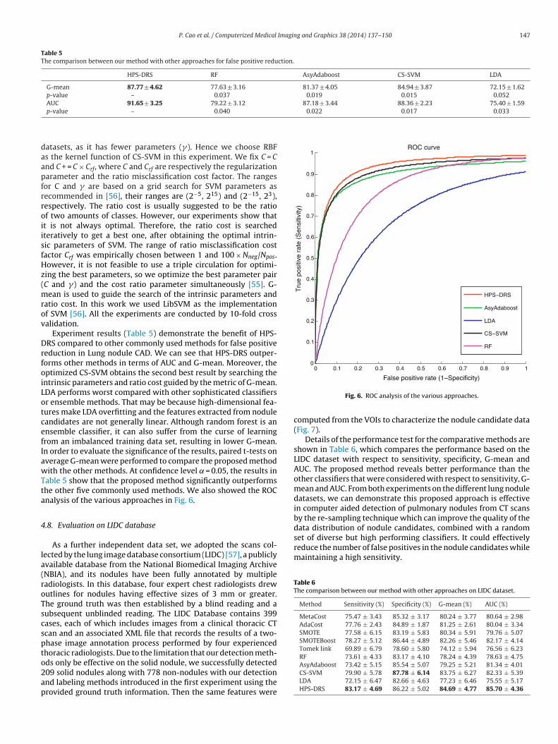
Table 5The comparison between our method with other approaches for false positive reduction.

HPS-DRS RF AsyAdaboost CS-SVM LDA

G-mean 87.77 ± 4.62 77.63 ± 3.16 81.37 ± 4.05 84.94 ± 3.87 72.15 ± 1.62p-value – 0.037 0.019 0.015 0.052AUC 91.65 ± 3.25 79.22 ± 3.12 87.18 ± 3.44 88.36 ± 2.23 75.40 ± 1.59

0.022 0.017 0.033

daapfrroiisfHz(mrov

DrfoiLotcefIawTta

4

la(roTscspto2ap

0 0.1 0.2 0.3 0.4 0.5 0.6 0.7 0.8 0.9 10

0.1

0.2

0.3

0.4

0.5

0.6

0.7

0.8

0.9

1

False positive rate (1−Specificity)

Tru

e po

sitiv

e ra

te (

Sen

sitiv

ity)

ROC curve

HPS−DRS

AsyAdaboost

LDA

CS−SVM

RF

set of diverse but high performing classifiers. It could effectivelyreduce the number of false positives in the nodule candidates whilemaintaining a high sensitivity.

Table 6The comparison between our method with other approaches on LIDC dataset.

Method Sensitivity (%) Specificity (%) G-mean (%) AUC (%)

MetaCost 75.47 ± 3.43 85.32 ± 3.17 80.24 ± 3.77 80.64 ± 2.98AdaCost 77.76 ± 2.43 84.89 ± 1.87 81.25 ± 2.61 80.04 ± 3.34SMOTE 77.58 ± 6.15 83.19 ± 5.83 80.34 ± 5.91 79.76 ± 5.07SMOTEBoost 78.27 ± 5.12 86.44 ± 4.89 82.26 ± 5.46 82.17 ± 4.14Tomek link 69.89 ± 6.79 78.60 ± 5.80 74.12 ± 5.94 76.56 ± 6.23RF 73.61 ± 4.33 83.17 ± 4.10 78.24 ± 4.39 78.63 ± 4.75

p-value – 0.040

atasets, as it has fewer parameters (�). Hence we choose RBFs the kernel function of CS-SVM in this experiment. We fix C = Cnd C + = C × Crf, where C and Crf are respectively the regularizationarameter and the ratio misclassification cost factor. The rangesor C and � are based on a grid search for SVM parameters asecommended in [56], their ranges are (2−5, 215) and (2−15, 23),espectively. The ratio cost is usually suggested to be the ratiof two amounts of classes. However, our experiments show thatt is not always optimal. Therefore, the ratio cost is searchedteratively to get a best one, after obtaining the optimal intrin-ic parameters of SVM. The range of ratio misclassification costactor Crf was empirically chosen between 1 and 100 × Nneg/Npos.owever, it is not feasible to use a triple circulation for optimi-ing the best parameters, so we optimize the best parameter pairC and �) and the cost ratio parameter simultaneously [55]. G-

ean is used to guide the search of the intrinsic parameters andatio cost. In this work we used LibSVM as the implementationf SVM [56]. All the experiments are conducted by 10-fold crossalidation.

Experiment results (Table 5) demonstrate the benefit of HPS-RS compared to other commonly used methods for false positive

eduction in Lung nodule CAD. We can see that HPS-DRS outper-orms other methods in terms of AUC and G-mean. Moreover, theptimized CS-SVM obtains the second best result by searching thentrinsic parameters and ratio cost guided by the metric of G-mean.DA performs worst compared with other sophisticated classifiersr ensemble methods. That may be because high-dimensional fea-ures make LDA overfitting and the features extracted from noduleandidates are not generally linear. Although random forest is annsemble classifier, it can also suffer from the curse of learningrom an imbalanced training data set, resulting in lower G-mean.n order to evaluate the significance of the results, paired t-tests onverage G-mean were performed to compare the proposed methodith the other methods. At confidence level ̨ = 0.05, the results in

able 5 show that the proposed method significantly outperformshe other five commonly used methods. We also showed the ROCnalysis of the various approaches in Fig. 6.

.8. Evaluation on LIDC database

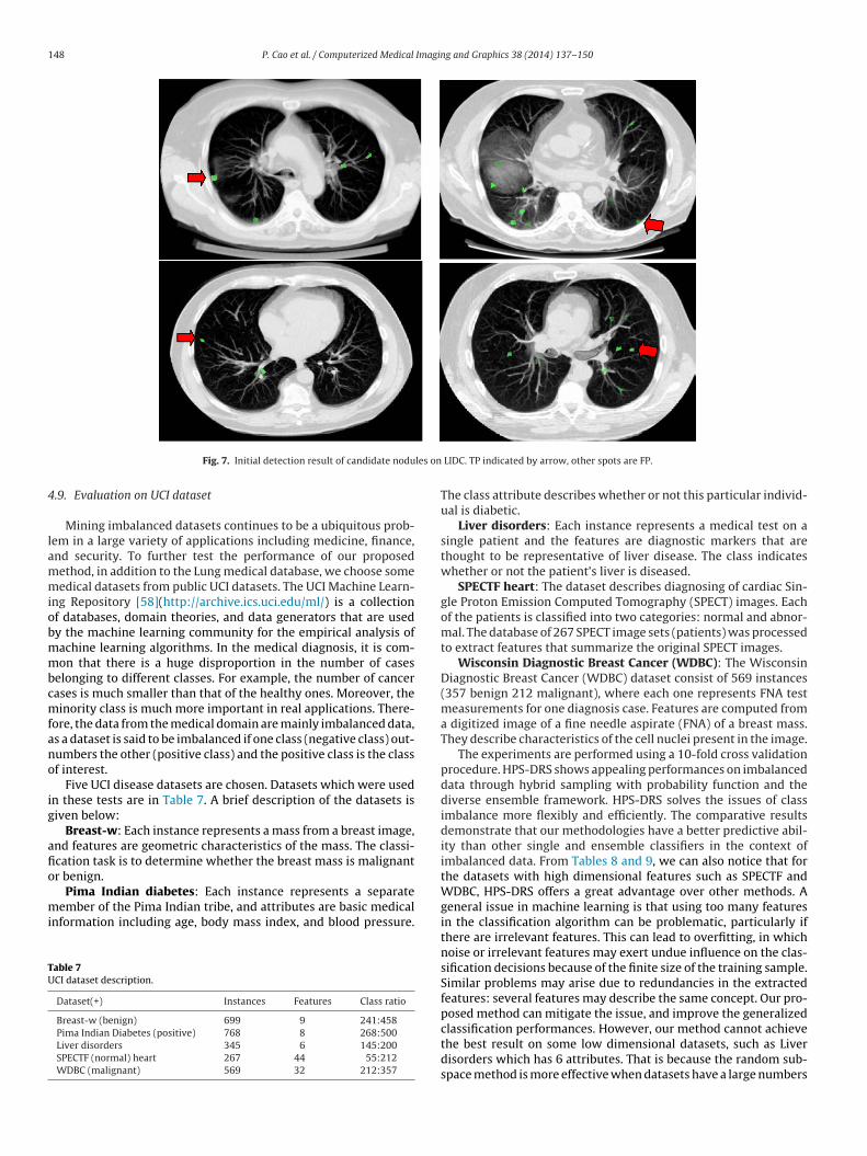
As a further independent data set, we adopted the scans col-ected by the lung image database consortium (LIDC) [57], a publiclyvailable database from the National Biomedical Imaging ArchiveNBIA), and its nodules have been fully annotated by multipleadiologists. In this database, four expert chest radiologists drewutlines for nodules having effective sizes of 3 mm or greater.he ground truth was then established by a blind reading and aubsequent unblinded reading. The LIDC Database contains 399ases, each of which includes images from a clinical thoracic CTcan and an associated XML file that records the results of a two-hase image annotation process performed by four experiencedhoracic radiologists. Due to the limitation that our detection meth-

ds only be effective on the solid nodule, we successfully detected09 solid nodules along with 778 non-nodules with our detectionnd labeling methods introduced in the first experiment using therovided ground truth information. Then the same features were

Fig. 6. ROC analysis of the various approaches.

computed from the VOIs to characterize the nodule candidate data(Fig. 7).

Details of the performance test for the comparative methods areshown in Table 6, which compares the performance based on theLIDC dataset with respect to sensitivity, specificity, G-mean andAUC. The proposed method reveals better performance than theother classifiers that were considered with respect to sensitivity, G-mean and AUC. From both experiments on the different lung noduledatasets, we can demonstrate this proposed approach is effectivein computer aided detection of pulmonary nodules from CT scansby the re-sampling technique which can improve the quality of thedata distribution of nodule candidates, combined with a random

AsyAdaboost 73.42 ± 5.15 85.54 ± 5.07 79.25 ± 5.21 81.34 ± 4.01CS-SVM 79.90 ± 5.78 87.78 ± 6.14 83.75 ± 6.27 82.33 ± 5.39LDA 72.15 ± 6.47 82.66 ± 4.63 77.23 ± 6.46 75.55 ± 5.17HPS-DRS 83.17 ± 4.69 86.22 ± 5.02 84.69 ± 4.77 85.70 ± 4.36

148 P. Cao et al. / Computerized Medical Imaging and Graphics 38 (2014) 137– 150

les on

4

lammiobmmbcmfano

ig

afio

mi

TU

Fig. 7. Initial detection result of candidate nodu

.9. Evaluation on UCI dataset

Mining imbalanced datasets continues to be a ubiquitous prob-em in a large variety of applications including medicine, finance,nd security. To further test the performance of our proposedethod, in addition to the Lung medical database, we choose someedical datasets from public UCI datasets. The UCI Machine Learn-

ng Repository [58](http://archive.ics.uci.edu/ml/) is a collectionf databases, domain theories, and data generators that are usedy the machine learning community for the empirical analysis ofachine learning algorithms. In the medical diagnosis, it is com-on that there is a huge disproportion in the number of cases

elonging to different classes. For example, the number of cancerases is much smaller than that of the healthy ones. Moreover, theinority class is much more important in real applications. There-

ore, the data from the medical domain are mainly imbalanced data,s a dataset is said to be imbalanced if one class (negative class) out-umbers the other (positive class) and the positive class is the classf interest.

Five UCI disease datasets are chosen. Datasets which were usedn these tests are in Table 7. A brief description of the datasets isiven below:

Breast-w: Each instance represents a mass from a breast image,nd features are geometric characteristics of the mass. The classi-cation task is to determine whether the breast mass is malignantr benign.

Pima Indian diabetes: Each instance represents a separateember of the Pima Indian tribe, and attributes are basic medical

nformation including age, body mass index, and blood pressure.

able 7CI dataset description.

Dataset(+) Instances Features Class ratio

Breast-w (benign) 699 9 241:458Pima Indian Diabetes (positive) 768 8 268:500Liver disorders 345 6 145:200SPECTF (normal) heart 267 44 55:212WDBC (malignant) 569 32 212:357

LIDC. TP indicated by arrow, other spots are FP.

The class attribute describes whether or not this particular individ-ual is diabetic.

Liver disorders: Each instance represents a medical test on asingle patient and the features are diagnostic markers that arethought to be representative of liver disease. The class indicateswhether or not the patient’s liver is diseased.

SPECTF heart: The dataset describes diagnosing of cardiac Sin-gle Proton Emission Computed Tomography (SPECT) images. Eachof the patients is classified into two categories: normal and abnor-mal. The database of 267 SPECT image sets (patients) was processedto extract features that summarize the original SPECT images.

Wisconsin Diagnostic Breast Cancer (WDBC): The WisconsinDiagnostic Breast Cancer (WDBC) dataset consist of 569 instances(357 benign 212 malignant), where each one represents FNA testmeasurements for one diagnosis case. Features are computed froma digitized image of a fine needle aspirate (FNA) of a breast mass.They describe characteristics of the cell nuclei present in the image.

The experiments are performed using a 10-fold cross validationprocedure. HPS-DRS shows appealing performances on imbalanceddata through hybrid sampling with probability function and thediverse ensemble framework. HPS-DRS solves the issues of classimbalance more flexibly and efficiently. The comparative resultsdemonstrate that our methodologies have a better predictive abil-ity than other single and ensemble classifiers in the context ofimbalanced data. From Tables 8 and 9, we can also notice that forthe datasets with high dimensional features such as SPECTF andWDBC, HPS-DRS offers a great advantage over other methods. Ageneral issue in machine learning is that using too many featuresin the classification algorithm can be problematic, particularly ifthere are irrelevant features. This can lead to overfitting, in whichnoise or irrelevant features may exert undue influence on the clas-sification decisions because of the finite size of the training sample.Similar problems may arise due to redundancies in the extractedfeatures: several features may describe the same concept. Our pro-posed method can mitigate the issue, and improve the generalized

classification performances. However, our method cannot achievethe best result on some low dimensional datasets, such as Liverdisorders which has 6 attributes. That is because the random sub-space method is more effective when datasets have a large numbers

P. Cao et al. / Computerized Medical Imaging and Graphics 38 (2014) 137– 150 149

Table 8The comparison between our method with other approaches on UCI dataset.

Dataset Metric MetaCost AdaCost SMOTE SMOTEBoost Tomek link

Breast-w G-mean 0.942 0.966 0.970 0.972 0.964AUC 0.951 0.969 0.962 0.976 0.920

Pima G-mean 0.741 0.738 0.744 0.741 0.720AUC 0.846 0.867 0.863 0.864 0.838

Liver disorders G-mean 0.607 0.612 0.629 0.645 0.603AUC 0.803 0.819 0.826 0.835 0.794

SPECTF heart G-mean 0.771 0.766 0.769 0.773 0.707AUC 0.872 0.887 0.871 0.874 0.855

WDBC G-mean 0.910 0.923 0.951 0.967 0.917AUC 0.952 0.964 0.982 0.993 0.955

Table 9The comparison between our method with other approaches on UCI dataset.

Dataset Metric Random forest AsyAdaboost CS-SVM LDA HPS-DRS

Breast-w G-mean 0.972 0.958 0.988 0.919 0.976AUC 0.933 0.953 0.986 0.931 0.986

Pima G-mean 0.727 0.752 0.758 0.708 0.779AUC 0.862 0.851 0.884 0.853 0.887

Liver disorders G-mean 0.594 0.609 0.655 0.578 0.629AUC 0.782 0.799 0.837 0.779 0.831

SPECTF Heart G-mean 0.745 0.763 0.819 0.705 0.8260.80.90.9

arscscd

5

Lawwwosspcmtnoe

A

MdC

R

[

[

[

[

[

[

[

[

[

AUC 0.872

WDBC G-mean 0.887

AUC 0.941

ttributes. With a very small number of attributes, each classifiereceives a small set of features and thus is weak. The CS-SVM clas-ifier performs satisfactorily for some data relatively easy to belassified. However, it cannot achieve an expected performance onome complex data, and the optimization of parameters is timeonsuming. Empirical evaluation on a wide variety of imbalancedatasets establishes the superiority of the new algorithm.

. Conclusion

The false positive reduction is a class imbalance task in theung nodule detection. In this paper, we have proposed a newlgorithm, hybrid probabilistic sampling method combined witheighted random subspace methods. DRS is an effective frame-ork for imbalanced data learning as it provides varied subsets andeighted voting according to each classifier performance. More-

ver, HPS can solve the between-class and within-class imbalanceimultaneously. Through theoretical justifications and empiricaltudies, we demonstrated the effectiveness of the method on theerformance of reducing false positives. The methods proposedould be applied on many other potential lesion detection, such asass, polyp, and microcalcification. Moreover, it can also be applied

o other machine learning problems such as computer-aided diag-osis. Furthermore, in this paper, our methods are only evaluatedn binary class imbalanced classification. In the future, we willxtend our methods to multi-class imbalanced classification.

cknowledgments

This work is supported by the Alberta Innovates Centre forachine Learning as well as the National Natural Science Foun-

ation of China (61001047) and one author was supported by thehina Scholarship Council for two years at the University of Alberta.

eferences

[1] Jemal A, Murray T, Ward E, Samuels A, Tiwari RC, Ghafoor A, et al. Cancerstatistics, 2005. CA: A Cancer Journal for Clinicians 2005;55(1):10–30.

[2] Cancer Facts and Figures 2012. The American Cancer Society 2012.

[

[

81 0.893 0.830 0.88202 0.959 0.863 0.97544 0.987 0.922 0.993

[3] Austin JH, Müller NL, Friedman PJ, Hansell DM, Naidich DP, Remy-Jardin M, et al.Glossary of terms for CT of the lungs: recommendations of the NomenclatureCommittee of the Fleischner Society. Radiology 1996;200(2):327–31.

[4] Li Q. Recent progress in computer-aided diagnosis of lung nod-ules on thin-section CT. Computerized Medical Imaging and Graphics2007;31(4–5):248–57.

[5] Temesguen M, Russell CH, Steven KR. A new computationally efficient CADsystem for pulmonary nodule detection in CT imagery. Medical Image Analysis2010;14:390–406.

[6] Gomathi M, Thangaraj P. Computer aided medical diagnosis system for detec-tion of lung cancer nodules: a survey. International Journal of ComputationalIntelligence Research 2009;5(4):453–62.

[7] Dhara AK, Mukhopadhyay S, Khandelwal N. Computer-aided detection andanalysis of pulmonary nodule from CT images: a survey. IETE Technical Review2012;29(4):265–75.

[8] Boroczky L, Zhao LZ, Lee KP. Feature subset selection for improving the per-formance of false positive reduction in lung nodule CAD. IEEE Transactions onInformation Technology in Biomedicine 2006;10(3):504–11.

[9] Choi WK, Choi TS. Genetic programming-based feature transform and clas-sification for the automatic detection of pulmonary nodules on computedtomography images. Information Sciences 2012;212(1):57–78.

10] Suzuki K, Armato SG, Li F, Sone S, Doi K. Massive training artificial neural net-work for reduction of false positives in computerized detection of lung nodulesin low-dose computed tomography. Medical Physics 2003;30:1602–17.

11] Ge Z, Sahiner B, Chan HP, Hadjiiski LM, Wei J, Bogot N, et al. Computer aideddetection of lung nodules: false positive reduction using a 3-D gradient fieldmethod. In: Proceedings of SPIE 5370. 2004. p. 1076–82.

12] Yang M, Periaswamy S, Wu Y. False positive reduction in lung GGO noduledetection with 3D volume shape descriptor. In: IEEE international conferenceon acoustics, speech and signal processing, vol. 1. 2007. p. 437–40.

13] Melli G, Wu X, Beinat P, Bonchi F, Cao L, Duan R, et al. Top-10 data mining casestudies. International Journal of Information Technology and Decision Making2012;11(2):389–400.

14] Chawla NV, Japkowicz N, Kotcz A. Editorial: special issue on learning fromimbalanced data sets. ACM SIGKDD Explorations Newsletter 2004;6(1):1–6.

15] He H, Garcia E. Learning from imbalanced data. IEEE Transactions on Knowledgeand Data Engineering 2009;21(9):1263–84.

16] Mazurowski MA, Habas PA, Zurada JM, Lo JY, Baker JA, Tourassi GD. Train-ing neural network classifiers for medical decision making: the effectsof imbalanced datasets on classification performance. Neural Networks2008;21(2–3):427–36.

17] Rao RB, Fung G, Krishnapuram B, Bi J, Dundar M, Raykar V, et al. Mining medicalimages. In: Proceedings of the third workshop on data mining case studies andpractice prize, fifteenth annual SIGKDD international conference on knowledgediscovery and data mining. 2009.

18] Ren J. ANN vs. SVM: which one performs better in classification of MCCS inmammogram imaging. Knowledge-Based Systems 2012;26:144–53.

19] Yang X, Zheng Y, Siddique M, Beddoe G. Learning from imbalanced data: acomparative study for colon CAD. In: Proceedings of the SPIE. 2008. p. 6915.

20] Malof JM, Mazurowski MA, Tourassi GD. The effect of class imbalance on caseselection for case-based classifiers: an empirical study in the context of medicaldecision support. Neural Networks 2012;25:141–5.

1 Imagin

[

[

[

[

[

[

[

[

[

[

[

[

[

[

[

[

[

[

[

[

[

[

[

[

[

[

[

[

[

[[

[

[

[

[

[

[

[

50 P. Cao et al. / Computerized Medical

21] Yang Q, Wu X. 10 challenging problems in data mining research. InternationalJournal of Information Technology & Decision Making 2006;5(4):597–604.

22] Weiss G. The impact of small disjuncts on classifier learning. Annals of Infor-mation Systems 2010;5(8):193–226.

23] Jo T, Japkowicz N. Class imbalances versus small disjuncts. ACM SIGKDD Explo-rations Newsletter 2004;6(1):40–9.

24] Holte RC, Acker LE, Porter BW. Concept learning and the problem of small dis-juncts. In: Proceedings of the 7th international joint conference on artificialintelligence. 1989. p. 813–8.

25] Lusa L. Class prediction for high-dimensional class-imbalanced data. BMCBioinformatics 2010;11(1):523–41.

26] Ho T. The random subspace method for constructing decision forests. IEEETransactions on Pattern Analysis and Machine Intelligence 1998;20(8):832–44.

27] Li Q, Doi K. Analysis and minimization of overtraining effect in rule-basedclassifiers for computer-aided diagnosis. Medical Physics 2006;33:320–8.

28] Tao Y, Lu L, Dewan H, Chen A, Corso J, Xuan J, et al. Multi-level ground glassnodule detection and segmentation in CT lung images. In: Medical image com-puting and computer-assisted intervention-MICCAI. 2009. p. 715–23.

29] Jiang J, Trundle P, Ren J. Medical image analysis with artificial neural networks.Computerized Medical Imaging and Graphics 2010;34(8):617–31.

30] Wang Q, Kang W, Wu C, Wang B. Computer-aided detection of lung nodules bySVM based on 3D matrix patterns. Clinical Imaging 2013;37(1):62–9.

31] Campadelli P, Casiraghi E, Valentini G. Support vector machines for candidatenodules classification. Neurocomputing 2005;68:281–8.

32] Lee SLA, Kouzani AZ, Hu EJ. Random forest based lung nodule classifi-cation aided by clustering. Computerized Medical Imaging and Graphics2010;34(7):535–42.

33] Dolejsi M, Kybic J, Tuma S, Polovincák M. Reducing false positive responsesin lung nodule detector system by asymmetric Adaboost newblock. In:Proceedings of fifth IEEE international symposium on biomedical imaging ISBI.2008. p. 656–9.

34] Chawla NV, Bowyer KW, Hall LO, Kegelmeyer WP. SMOTE: syntheticminority over-sampling technique. Journal of Artificial Intelligence Research2002;16(1):321–57.

35] Ramentol E, Caballero Y, Bello R, Herrera F. SMOTE-RSB*: a hybrid preprocess-ing approach based on oversampling and undersampling for high imbalanceddata-sets using smote and rough sets theory. Knowledge and Information Sys-tems 2012;33(2):245–65.

36] Chawla NV, Lazarevic A, Hall LO, Bowyer KW. SMOTEBoost: improving predic-tion of the minority class in boosting. In: Knowledge discovery in databases:PKDD. 2003. p. 107–19.

37] Wang BX, Japkowicz N. Boosting support vector machines for imbalanced datasets. Knowledge and Information Systems 2010;25(1):1–20.

38] Sun Y, Kamel MS, Wang Y. Boosting for learning multiple classes with imbal-anced class distribution. In: Proceedings of the sixth international conferenceon data mining. 2006. p. 592–602.

39] Zhou ZH, Liu XY. Training cost-sensitive neural networks with methodsaddressing the class imbalance problem. IEEE Transactions on Knowledge andData Engineering 2006;18(1):63–77.

40] Galar M, Fernandez A, Barrenechea E, Bustince H, et al. A review on ensem-bles for the class imbalance problem: bagging-, boosting-, and hybrid-basedapproaches. IEEE Transactions on Systems, Man, and Cybernetics, Part C2012;42:463–84.

41] Liu XY, Wu J, Zhou ZH. Exploratory undersampling for class-imbalance learn-ing. IEEE Transactions on Systems, Man, and Cybernetics, Part B: Cybernetics2009;39(2):539–50.

42] Fan W, Stolfo SJ, Zhang J, Chan PK. AdaCost: misclassification cost-sensitiveboosting. In: Proceedings of international conference machine learning. 1999.p. 97–105.

43] Domingos P. MetaCost: a general method for making classifiers cost-sensitive.

In: Proceedings of the fifth ACM SIGKDD international conference on knowl-edge discovery and data mining. 1999. p. 155–64.

44] Figueiredo MAT, Jain AK, Doi K. Unsupervised learning of finite mixturemodels. IEEE Transactions on Pattern Analysis and Machine Intelligence2002;24(3):381–96.

g and Graphics 38 (2014) 137– 150

45] Denil M, Trappenberg T. Overlap versus imbalance. In: Proceedings of the 23rdCanadian conference on advances in artificial intelligence. 2010. p. 220–31.

46] Li Q, Sone S, Doi K. Selective enhancement filters for nodules, vessels,and airway walls in two-and three-dimensional CT scans. Medical Physics2003;30:2040–51.

47] Li Q, Li F, Doi K. Computerized detection of lung nodules in thin-section CTimages by use of selective enhancement filters and an automated rule-basedclassifier. Academic Radiology 2008;15(2):165–75.

48] Lu X, Wei GQ, Qian J, Jain AK. Learning-based pulmonary nodule detection frommultislice CT data. In: Proceedings of CARS 2004 computer assisted radiologyand surgery. 2004. p. 1356–63.

49] Yoshida H, Nappi J. Three-dimensional computer-aided diagnosis schemefor detection of colonic polyps. IEEE Transactions on Medical Imaging2001;20(12):1261–74.

50] Koenderink JJ. Solid shape. Cambridge: Cambridge University Press; 1990.51] Kawata Y, Niki H, Ohmatsu H, Kakinuma R, Eguchi K, Kaenko M, et al. Quanti-

tative surface characterization of pulmonary nodules based on thin-section CTimages. IEEE Transactions on Nuclear Science 1998;45(4):2132–8.

52] Kobatake H, Murakami M. Adaptive filter to detect rounded convex regions: Irisfilter. In: Proceedings of the 13th international conference on pattern recogni-tion. 1996. p. 340–4.

53] Wu WJ, Lin SWH, Moon WK. Combining support vector machine with geneticalgorithm to classify ultrasound breast tumor images. Computerized MedicalImaging and Graphics 2012;36:627–33.

54] Tomek I. Two modifications of CNN. IEEE Transactions on Systems, Man, andCybernetics 1976;6:769–72.

55] Cao P, Zhao DZ, Zaiane O. An optimized cost-sensitive SVM for imbalanceddata learning. In: Proceedings of the 17th Pacific-Asia conference on knowledgediscovery and data mining. 2013. p. 280–92.

56] Hsu CW, Chang CC, Lin CJ. A practical guide to support vector classification;2003.

57] McNitt-Gray MF, Armato SG, Meyer CR, Reeves AP, et al. The lung imagedatabase consortium (LIDC) data collection process for nodule detection andannotation. Academic Radiology 2007;14:1464–74.

58] Asuncion G, Newman D. UCI machine learning repository; 2007.

Peng Caois a PhD student enrolled in the Northeastern University, China. Peng hasbeen working with the Alberta Innovates Center for Machine Learning (AICML) –computing science at the University of Alberta, since 2011. Peng received an MScin computer science from Northeastern University, China, in 2005. His researchinterests are imbalanced data learning, medical image mining.

Jinzhu Yang received his PhD in computer science from Northeastern University,in 2007. Jinzhu is an associate professor in the College of Information Science andEngineering, Northeastern University.

Wei Li received his Master in computer science from Northeastern University, in2006. Wei is an associate director in Key Laboratory of Medical Image Computing ofthe Chinese Ministry of Education.

Dazhe Zhao received her PhD in computer science from Berlin Institute of Technol-ogy, Germany, in 1996. Dazhe is a professor in the College of Information Science andEngineering, Northeastern University, and the director in Key Laboratory of MedicalImage Computing of the Chinese Ministry of Education. She is also the president ofthe Research Institute of Neusoft Corporation.

Osmar Zaiane received his PhD in computing science from Simon Fraser University,Canada, in 1999 specializing in data mining. He is a professor at the University ofAlberta, Canada, with research interest in novel data mining techniques and cur-rently focuses on social network analysis as well as health informatics applications.He is the scientific director of AICML (Alberta Innovates Centre for Machine Learn-

ing). He regularly serves on the program committees of international conferences inthe field of knowledge discovery and data mining and was the program co-chair forthe IEEE international conference on data mining ICDM’2007, and the general chairfor ICDM’2011. He is the associate editor of knowledge and information systems anddata mining and knowledge discovery.